On Exploiting Tile Partitioning to Reduce Bitrate and Processing Time in VVC Surveillance Streams with Object Detection

Abstract

One of the main targets in video surveillance systems is to detect and possibly identify objects within monitoring range. This entails analyzing the video stream, by applying object detection techniques on one or more frames. Regardless of the output, the stream is usually archived for future use. Real-time requirements, network bandwidth, and storage constraints play a significant role to total performance. As video resolution increases, so does the video stream size. To harness such an increase, newer video compression standards offer sophisticated coding tools that aim at reducing video size, with minimal quality loss. However, as the achievable compression ratio increases, so does the computational complexity. In this paper, we propose a methodology to reduce both bitrate and processing time of video surveillance streams whereby object detection is performed. The method takes advantage of tile partitioning, with the aim of (i) reducing the scope and the invocation frequency of the object detection module, (ii) encoding different blocks of a frame at different quality levels, depending on whether objects exist or not, and (iii) encoding and transmitting only tiles containing objects. Experimental results using the UA-DETRAC dataset and the VVenC encoder demonstrate that exploiting tile partitioning in the manner proposed in the paper results in reducing bitrate and processing time at the expense of only tiny losses in accuracy.

1. Introduction

Undoubtedly, video surveillance systems are key components to security infrastructure, with their preventative effects being well documented, e.g., ref. [1] reports a 25% crime decrease in parking lots and a 10% decrease in town centres. Furthermore, the contribution of video surveillance archives to forensic analysis of security events cannot be understated. Of particular importance to such systems is the ability to quickly identify (and possibly recognize and track) new objects entering the monitored area. This is conducted by analyzing the captured frames, nowadays with the use of Deep Neural Networks (DNNs). Naturally, as video resolution increases, so does the potential object detection accuracy of the DNN, but also the computational overhead of it. Even more, higher resolutions mean higher bandwidth and storage demands, respectively, for transmission and archiving. Since transmitting and storing raw video data is not a valid option due to immense size, codecs are used.

Research on video coding standards has been avid in the past years. From the Blu-ray era Advanced Video Coding (AVC) [2] to its successor, High Efficieny Video Coding (HEVC) [3], and nowadays the 8K era Versatile Video Coding (VVC) [4], the challenge has always been the same, namely, to provide high compression rate, while incurring minimal quality loss. In order to achieve the aforementioned purpose, the frame is split into blocks of pixels, e.g., macroblocks of 16 × 16 pixels in H.264/AVC, Coding Tree Units (CTUs) of up to 64 × 64 pixels in HEVC and 128 × 128 in VVC. Spatial and temporal redundancies among blocks (or parts of them) are identified and exploited to achieve compression. Unfortunately, this comes at a high computational cost, especially as far as newer standards are concerned, since they employ more sophisticated methods to improve coding efficiency. For instance, as reported by [5], compared to HEVC, the VVC standard achieves roughly 50% more compression ratio for the same video quality, but at a tenfold increase in processing time.

Harnessing the computational overhead of video coding standards is of paramount importance for video streaming and teleconferencing. However, it becomes even more important in the video surveillance domain, since it interplays with higher video resolutions, object detection accuracy, archive storage space, bandwidth and real time criteria, in order to define system’s performance as a whole. To speed up the process, in the related literature, both parallelization was proposed at various levels in [6,7], and decision tree pruning at various coding steps [8]. Although such techniques are applicable in the context of a video surveillance system with object detection capabilities, the domain offers a distinct potential (compared to simple live streaming) for identifying what information is important within a frame and what is not. Namely, object-related information is highly important, while background scenery less so.

Driven by the above remark, in this paper, we aim to reduce the encoding time and bitrate (thus, needed bandwidth and storage space) of a surveillance stream by avoiding the encoding and transmission of areas unrelated to objects. To do so, we take advantage of the ability provided by new video coding standards to split a frame in a grid-like fashion into tiles. Tiles are rectangular areas comprised of multiple blocks and can be encoded and transmitted separately. Furthermore, we tackle the problem of when to invoke the DNN for object detection, since it plays an important role in system accuracy and processing time overhead. Last but not least, we judiciously use coding parameters to enhance quality where objects appear (or are estimated to appear). Our contributions include the following:

• We propose a tile partitioning scheme, with the aim of maximizing the area covered by tiles containing no objects; these tiles are skipped during encoding.
• We propose a scheme based on pixel variance to identify whether invocation of object detection module is needed or not.
• The CTUs (blocks) of a tile containing one or more objects are encoded with different quality parameters depending on whether they, in turn, contain an object or not; since objects might move, a variance based method is proposed to estimate the CTUs involved with object movement; the method is applicable in the interval between subsequent object detection invocations.

In combination, the above three schemes are able to reduce processing time overhead and bitrate, at only a small loss in object detection accuracy. Namely, using the Versatile Video Encoder (VVEnC) [9] for the VVC codec, Mask Region-based Convolutional Neural Network (MASK-RCNN) [10] for object detection, and the University at Albany Detection and Tracking (UA-DETRAC) dataset [11], an average reduction of more than 13% in processing time and 19% in bitrate were recorded against a default encoding scheme with identical coding parameters, performing no object detection. These results highlight the merits of our approach, especially since the comparison was against a scheme with no object detection overhead. Furthermore, these merits come at a very small loss in accuracy of roughly 1%. Comparison with simpler variations and related work further establishes our algorithm as a valid trade-off between accuracy and other performance metrics. Last but not least, we should note that our methodology is not Deep Neural Network (DNN)-dependent (any object detection module could be incorporated). It is also not video standard-dependent, as long as the standard supports tiles. For instance, it is applicable to both HEVC [3] and AOMedia Video 1 (AV1) [12].

The rest of this paper is organized as follows. Section 2 provides an overview of video coding. Section 3 discusses related work. Section 4 illustrates the algorithm proposed in this paper, which is experimentally evaluated in Section 5. Finally, Section 6 includes our concluding remarks.

2. Video Coding Overview

As with most compression methods, video encoding aims to exploit redundancies in data. Video encoding addresses spatial and temporal redundancies through hybrid encoding, obeying a trade-off between quality and compression rate. Firstly, each frame is divided into blocks. In AVC, macroblocks (MBs) were used, whereas in HEVC and VVC, CTUs are employed. The encoder then aims to find data redundancies in each block. The block structure offers content-adaptive capabilities, whereby a block can be further subdivided according to its visual complexity. MBs, whose original size is 16 × 16 pixels, can be divided up to 4 × 4 blocks, while CTUs, which can be up to 128 × 128 in size, can be quad, binary, or tertiary split in Coding Units (CUs). The splits available in VVC are depicted in Figure 1. CUs can be further split, with the minimum size of sub-blocks reaching 4 × 4.

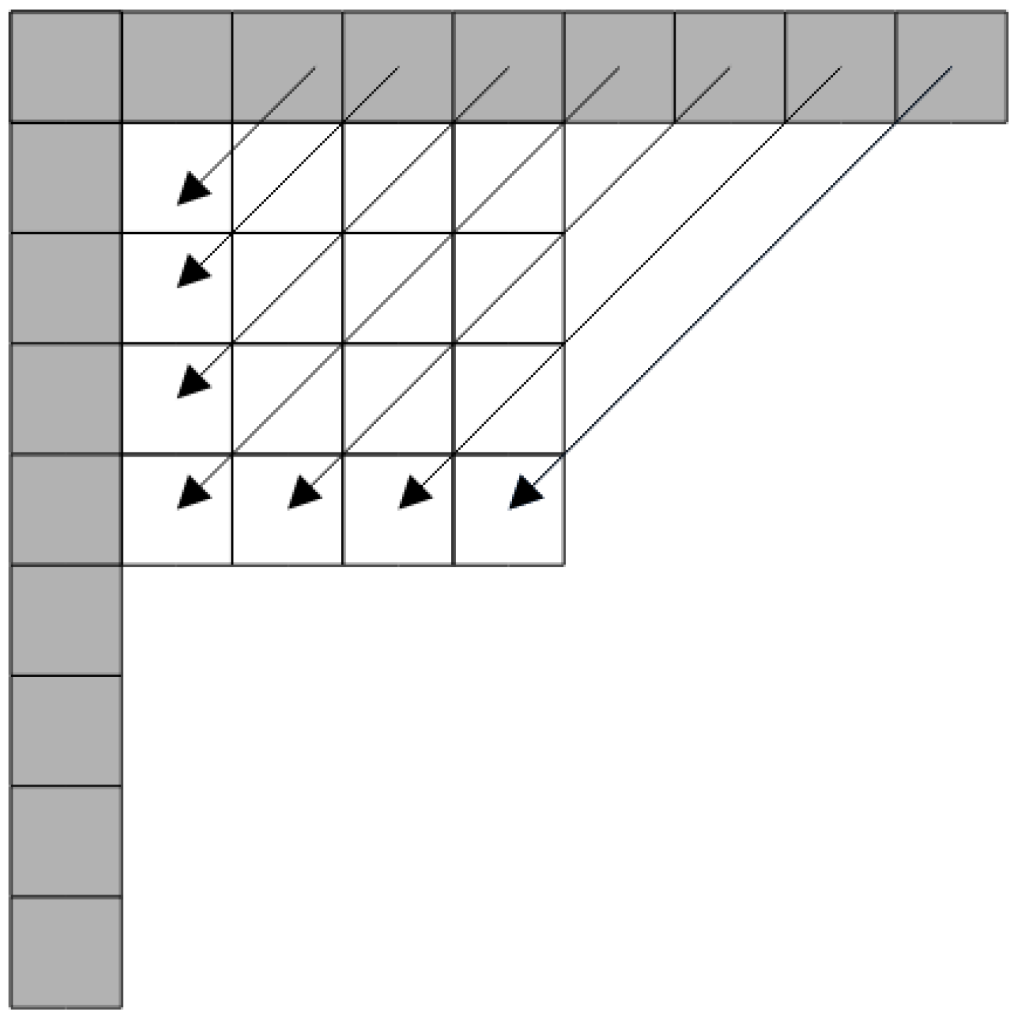
Spatial correlations are exploited through intra-frame encoding. In intra-frame encoding, instead of transmitting the pixel values of the block as is, we can infer the values of the pixels through reference pixels. The pixels from top, top left, and left neighboring blocks are used as reference, specifically the ones bordering the block to be encoded. Extrapolation of the original block from reference pixels is conducted using various methods called intra-prediction modes. For instance, in VVC, there exist 67 such modes. An example of how intra-prediction functions is shown in Figure 2. In principle, all modes are tested and the one achieving the best trade-off between perceptual loss and compression ratio is selected. Since reference pixels are already encoded in the stream, deriving the predicted block at the decoder side requires only transmitting the selected intra-mode.

Temporal redundancy is present in a video stream due to the fact that among consecutive frames large parts of a scenery remain almost unchanged. Inter-frame coding is employed in order to capitalize on the above. A block in the current frame is inter-predicted from previously encoded reference frames. In order to capture possible motion, a search area (typically consisting of surrounding blocks) is evaluated and the previous location at the reference frame of the block to be encoded is defined. Thus, deriving the prediction block on the decoder side requires only information about the location found, which is typically referred to as the Motion Vector (MV). Temporal redundancy is present throughout a video as the visual content in adjacent frames remains largely the same. In this case, inter-frame coding is employed. A block in the current frame is searched in previously coded frames. If the current block is located in a reference frame, then it can be inferred through the frame it was found in, alongside the corresponding MV.

Regardless of whether intra or inter-prediction is used to form the prediction block, differences between actual and predicted values must be tackled. For this reason, a residual block capturing these differences is calculated and transmitted. The residual block can be transmitted in a lossless or in a lossy manner, depending on the configuration of the compression rate/visual loss trade-off, whereby the error is transformed though Discrete Cosine Transform (DCT). In a lossy compression scenario, the Quantization Parameter (QP) is used by which the error can be quantized. As such, lower QPs yield higher quality at an expense in bitrate, whereas high QPs exhibit the opposite trend. In a hybrid encoding setting, a block can be coded through intra or inter-prediction with the most suitable solution being the one which minimizes cost J in Equation (1). Distortion is denoted by D, bitrate cost is represented with R, and $\lambda$ is a constant that represents the trade-off between quality and bitrate. All of the encoded information is then subjected to entropy coding to further reduce coding overhead.

$$J=D+\lambda ·R$$

(1)

High-level partitioning is present in video codecs enabling the selected transmission of parts of the frame together with parallelization, both at the encoder and the decoder side. The high-level structures present in VVC are tiles, slices, and subpictures. Tiles are rectangular areas of CTUs that form a tile grid, whereas slices are groups of CTUs that can be categorized as either rows of contiguous CTUs or rectangular areas. Subpictures are groups of slices offering higher degrees of independency and are mainly used in Virtual Reality (VR) settings. Lastly, frames are organized in Groups of Pictures (GOPs). The GOP structure has a fixed number of frames and typically remains unchanged throughout a video stream. Among others, the GOP structure defines reference dependencies among frames. Frames are characterized depending on the prediction scheme used as I-Frames, P-frames, and B-frames. I-frames are intra-predicted, whereas in P- and B-frames inter-prediction is used based on one or two reference frames, respectively.

3. Related Work

Our work is in the context of intelligent surveillance systems, whereby camera feeds are processed in an automatic manner, in order to identify objects and events of interest. Object detection has received significant research effort in the past varying from methods related to a single image in [13,14], up to detecting and tracking moving objects in a video feed in [15,16]. Various neural networks have been proposed for the problem, with more recent efforts concentrating on DNNs, e.g., refs. [10,17,18,19]. Of larger scope is research focusing directly on identifying security events. For instance, in [20,21], DNNs are used in order to classify video frames as regular or irregular and subsequently generate security alarm events. Regardless of the scope, common to the aforementioned works is a general processing pattern whereby the frames of a video stream are processed by a neural network and then encoded by some video coding standard. Compared to the aforementioned works, our goal is different, namely, to optimize both processing time and bitrate in surveillance streams with automatic object detection. As such, from the standpoint of this paper, object detection is only a component whose particularities do not limit the applicability of our methodology. For the record, it was decided to incorporate the DNN proposed in [10], due to its wide use in the field.

In order to achieve the targeted optimizations, our algorithm is based on three main tools, namely, (a) tile partitioning in order to reduce the total encoded area, (b) differentiation of quality levels in CTU encoding depending on whether CTUs contain objects or not, and (c) sparing invocation of the DNN. Strictly speaking, each of the aforementioned tools can be found in the literature in some form.

Content-adaptive high-level frame partitioning in VVC is discussed in [22,23]. In [22], the goal is to identify and group together regions of interest into tiles and subpictures with the aim of improving quality, while [23] discusses (among others) tile partitioning as a means to parallelize the encoding process. In this paper, tile partitioning is performed with the aim of maximizing the total area that will be skipped in the encoding process, due to the fact that it contains no objects.

As far as CTU coding is concerned, there exist two main research directions that are complementary to our work. The first aims to speed up the process by pruning decisions at tree partitioning level [24], at intra-mode level [8], etc. In the paper, we take advantage of the corresponding optimizations implemented by the encoder’s Low Delay Fast setting. The other direction concerns quality and bitrate trade-offs. Refs. [25,26] are works advocating saliency-driven encoding whereby low information CTUs are encoded at lower quality. For surveillance videos, ref. [27] explores spatiotemporal relations between blocks containing background and the ones containing objects, in order to provide better video feedback to object detection algorithms, while in [28], foreground and stationary background are encoded and stored independently and combined during the decoding phase. Moreover, the authors in [29] propose a downsampling/Super Resolution method explicitly trained for tasks such as object detection and semantic segmentation. Concerning suitable video configurations in traffic surveillance and dashcam video content, ref. [30] constructs a surveillance video system that tracks object movement and position while adapting the video coding configuration based both on content and network congestion. Similarly, ref. [31] proposes a deep reinforcement learning tool that adaptively selects a suitable video configuration, in order to balance the trade-off between bitrate and DNN analytic accuracy.

Finally, ref. [32] identifies regions of interest of objects in the frame and encodes such regions with a lower QP. This paper also capitalizes on saliency to improve bitrate on low information CTUs.

Summarizing, the works presented in the previous paragraph have a smaller scope compared to this paper, tackling components of the proposed optimization flow. Of interest are works in the context of multiple cameras. Ref. [33] proposes to encode from one Point Of View (POV) objects appearing in multiple feeds, while [34] tackles redundancies both for objects and background appearing in multiple POVs. The focus of this paper is different, tackling the optimization of a single feed, not only with regards to bitrate, but also processing time. Nevertheless, the proposed method in this paper is applicable to multiple feed processing and can be combined with the algorithms of [33,34] to further improve results.

Judging from motivation, perhaps the closest work to ours is [35], whereby the aim is to optimize bitrate and processing time. Here too, tile partitioning is used, with only tiles containing objects being encoded and transmitted. Towards this, a bitrate-based algorithm is proposed to estimate the tiles that contain objects. These tiles are afterwards sent to a DNN for object detection. Compared to [35], our approach differs in many ways. First of all, instead of assuming fixed tile partitioning, we use adaptive tile partitioning based on objects’ appearance. This is crucial, in order to better capture the dynamics of moving objects and enable more optimization opportunities. Secondly, we develop the heuristic to decide whether the DNN should be invoked or not. This heuristic is based on CTU variance calculation, which does not require prior CTU encoding, thus enduring small processing time. In contrast, in [35], all CTUs are first encoded and then the presence of objects at tiles is estimated based on bitrate. Finally, even within tiles that contain objects, there exist CTUs with background information. Contrary to [35], we capitalize on this fact to further reduce bitrate. To the best of our knowledge, this paper is the first to use both tile partitioning and salient-based coding, in order to achieve a composite optimization target of improving bitrate and processing time, while maintaining high coding quality in areas containing objects.

4. Algorithm

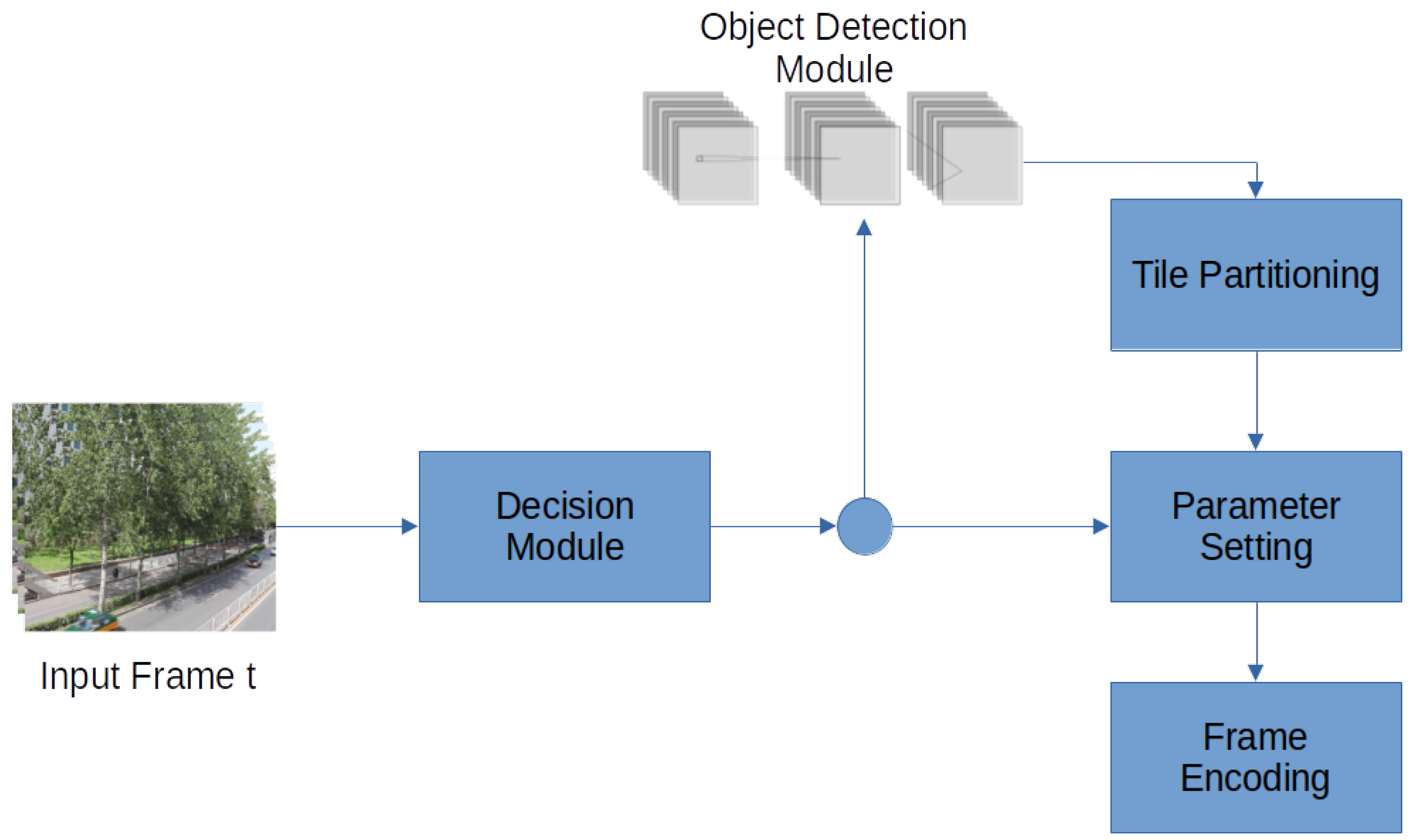
The algorithm proposed in this paper is invoked upon the arrival of each consecutive frame of a surveillance video. The processing involved is organized in a modular fashion, with the input being a raw frame and the final output being the encoded representation of it. The general flow of the algorithm is depicted in Figure 3. First, a Decision Module is activated, in order to determine whether object detection should be performed or not. In order to harness complexity, a positive decision does not affect the algorithmic flow immediately, but instead takes place at the starting frame of the next GOP. In this case, the object detection module consisting of the DNN presented in [10] will be invoked and the CTUs containing objects (or parts of them) will be marked. Then, the tile partitioning module will calculate a tile grid so as to minimize the total area of tiles containing marked CTUs. Regardless of whether object detection and tile partitioning are performed or not, the algorithm proceeds with the parameter setting module, which performs two main tasks. Firstly, it sets tiles containing no objects to Skip mode. Then, in the remaining ones, it selects different QP levels for each CTU, depending on whether they are marked or not. Since object detection is not performed on every frame, the detected objects at the beginning of a GOP might move on intermediate frames. For this reason, the parameter setting module uses the same QP level not only for the marked CTUs but also for adjacent ones that are estimated as possible object hosts. Finally, the encoding process takes place.

An example run of the algorithm is shown in Figure 4. Figure 4a shows the input frame and the CTU splitting of it, while Figure 4b shows which parts will be encoded and which ones will be skipped. As it can be observed (shaded areas), the object detection module recognizes the car in the bottom right, the pedestrian ahead of it, a bicycle rider in the right part, and the cars in the upper part of the frame as objects. It also identifies trees and the shades of them, the guard rail, and the lanes as background. Given the desired dimensions of the tile grid (3 × 3 in the example), the tile partitioning module defines tile boundaries so as to maximize the area of tiles that contain no objects and will be skipped. Following, we describe in detail the algorithmic modules.

4.1. Object Detection Module

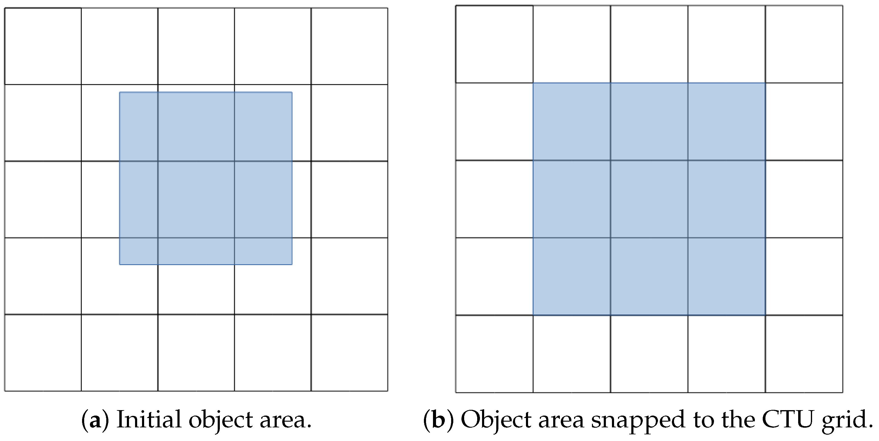
During this process, the frame is sent to the DNN. The DNN’s output consists of a mask as well as a minimum bounding box area for each object present in the image. We solely work with the bounding box areas of the objects. In order to comply with the VVC standard, we snap the rectangular areas of the objects to the CTU grid according to Equation (2), for an area a with a.x1 and a.x2 horizontal boundaries and a.y1 and a.y2 vertical boundaries in pixels, with size being the width/height of a CTU in pixels, forming the Snap function.

$$Snap\left(a\right)=(\lfloor {\displaystyle \frac{a.x1}{size}}\rfloor ,\lceil {\displaystyle \frac{a.x2}{size}}\rceil ,\lfloor {\displaystyle \frac{a.y1}{size}}\rfloor ,\lceil {\displaystyle \frac{a.y2}{size}}\rceil )$$

(2)

This way, we expand the area for an object derived from the DNN to contain CTUs that fully or partially overlap with said object. The snapped area coordinates are measured in CTUs. With this process, we essentially mark which CTUs in the frame contain objects. Figure 5 exhibits how this process functions. The marked CTUs in the form of $(i,j)$ coordinates along with the areas containing objects are then sent to the encoder by which the Tile Partitioning and the Parameter Setting Modules operate.

4.2. Decision Module

Object detection comes at a computational cost. Therefore, a per frame invocation strategy, although being the most adaptive in scene changes, might result in excessive processing delays. Moreover, many of these invocations might be redundant, since a total change of scene and object involvement on every frame is rather a seldom event. In this subsection, we describe the Decision Module which is responsible for defining whether object detection and subsequent optimizations (tile partitioning, etc.) should take place or not.

For the starting frame of the first GOP in the video sequence, object detection is invoked and subsequently tile partitioning occurs, whereby two tile categories are defined as follows: those which contain objects and those which do not. Regardless of the tile type, in the first frame, all tiles are encoded and transmitted; nevertheless, in subsequent frames, tiles with no objects are skipped. It is possible that at some point, a new object enters such a tile. To capture the case, for each CTU belonging to skipped tiles, the Decision Module computes the luma variance of its pixels in the current and the previous frame and calculates their absolute difference. If the absolute difference exceeds a threshold, it denotes the possible existence of a new coming object. Instead of performing object detection and tile adaptation instantly, we delay their invocation until the first frame of the subsequent GOP. In this way, tile structure remains constant within a GOP, which aids coding efficiency, while DNN invocations are limited to at most one per GOP. Undoubtedly, this is a trade-off that comes at the cost of reduced bitrate savings, which, as shown in the experiments, is minimal. As it pertains to the variance threshold, this is a tunable parameter. Its value should be small enough so as not to miss object movement and large enough to avoid being triggered by minor effects, such as rain, slight movements of camera, etc.

4.3. Tile Partitioning Module

Given the desired dimensions of the tile grid, M × N, and the output of the object detection module, which contains the rectangular areas of objects found within the frame, the tile partitioning module aims at defining the exact M − 1 horizontal and N− 1 vertical cuts that result in forming tiles so as to maximize the frame area that can be skipped during encoding. Specifically, the module takes as input all object boundaries, snapped to CTUs’ edges, together with the information for each CTU as to whether it contains an object or not. These boundaries form a tentative set of horizontal and vertical cuts, denoted by cutH and cutV, respectively. Encoders place restrictions on the minimum allowable tile size. For instance, in HEVC, a tile should consist of at least one row of two CTUs. Since it is recognized that extremely small tiles have an adverse effect on quality [36], but also in order to reduce complexity, we enforce a minimum tile size of 2 × 2 CTUs. This entails that all the selected cuts, either horizontal or vertical, should have a distance of at least two CTUs from each other. It also means that horizontal or vertical cuts just after the first row or column, respectively, are ineligible.

The two sets of tentative vertical and horizontal cuts (CutV and CutH) that were produced with the above methodology must be of size M and N, respectively. In case that the available eligible horizontal and vertical cuts are less than M − 1 or N− 1, respectively, we introduce eligible cuts to supplement the difference, according to the populateSet function shown in Algorithm 1. The function operates for both horizontal and vertical cuts. In the case of horizontal cuts, the algorithm takes as arguments set = CutH, bound = N, and sizeInCtu as the height of the frame in CTUs, whereas in the case of columns, the arguments are defined as set = CutV, bound = M, and sizeInCtu being the width of the frame in CTUs. populateSet works in iterations, each time adding one cut in a greedy manner, with the optimization criterion being the balancing of the distances between cuts.

Algorithm 1 PopulateSet(set,bound,sizeInCtu)

1: while  $set.length\left(\right)<bound-1$  do 2:     $minScore\leftarrow MAX\_INT$ 3:     for $candidateCut$ in $2..sizeInCtu$ do 4:         $score\leftarrow 0$ 5:         if $set.contains\left(candidateLine\right)$ then 6:            continue 7:         end if 8:         $tesCuts=set$ 9:         $testCuts.push\left(candidateLine\right)$ 10:         if $minDistanceBetweenLines\left(testCuts\right)<2$ then 11:            continue 12:         end if 13:         $a\leftarrow maxDistanceBetweenCuts\left(testCuts\right)$ 14:         $b\leftarrow minDistanceBetweenCuts\left(testCuts\right)$ 15:         $score\leftarrow a-b$ 16:         if $score<minScore$ then 17:            $bestCandidateCut\leftarrow candidateCut$ 18:            $minScore\leftarrow score$ 19:         end if 20:     end for 21:     $set.push\left(bestCandidateCut\right)$ 22: end while

After the populateSet process, we construct the possible M-1 and N-1 enumerations of CutH and cutV, which are stored into tileRowCombinations and tileColCombinations sets, respectively. Clearly, the candidate tile grids for consideration are the ones given by the Cartesian product of the two sets, |tileRowCombinations| × |tileColCombinations|. The enumeration process is a brute force approach that theoretically leads to intractable computations as M and N approach infinity. However, in practical cases, surveillance frames have limited boundaries and the computation is not only tractable, but also quite fast as discussed in the experiments.

Each candidate tile grid is evaluated with respect to the frame area that can be skipped during encoding. Specifically, the tiles containing no objects are identified and the number of the CTUs they contain acts as the optimization criterion (see Equation (3)), forming a Benefit function (denoted as B) that should be maximized. Surface is a function of a given tile t that calculates the area of said tile in CTUs, while NumOfObjects is a function of a tile t that calculates the number of objects being contained within said tile. In essence, the Benefit function calculates the areas of all tiles that contain no objects.

$$B=\sum _{t\in Tiles}Surface\left(t\right)|NumOfObjects\left(t\right)=0$$

(3)

The tile grid with the highest score is selected for implementation. Algorithm 2 illustrates the whole tile partitioning process in pseudocode. First, cutV and cutH are populated using object boundaries. This is conducted iteratively (lines 3–8), on the output of the Object Detection Module, dnn_areas. Then, the populateSet function is called to add candidates cuts if needed (lines 9–10). Afterwards, row and tile combinations are calculated in lines 9–14. The final tile-grid selection process takes place in lines 16–25, whereby the benefit of all possible tile-grid configurations is calculated and the configuration with the maximum benefit (maxBenefit) is selected. The output of our algorithm is stored in bestTileConfig, which contains the optimal tile grid. An example invocation of this process is shown in Figure 6.

Algorithm 2 TilePartitioning

1: $cutH\leftarrow \left\{\right\}$ 2: $cutV\leftarrow \left\{\right\}$ 3: for i in $dnn\_areas$ do 4:     $cutV.push(i.x1)$ 5:     $cutH.push(i.y1)$ 6:     $cutV.push(i.x2)$ 7:     $cutH.push(i.y2)$ 8: end for 9: $populateSet(cutH,M,widthInCTUs)$ 10: $populateSet(cutV,N,heightInCTUs)$ 11: $tileRowCombinations\leftarrow combsOfM\_minus1\left(cutH\right)$ 12: $tileRowCombinations\leftarrow excludeCombsWithMinDis(tileRowCombinations,2)$ 13: $tileColCombinations\leftarrow combsOfN\_minus1\left(cutV\right)$ 14: $tileColCombinations\leftarrow excludeCombsWithMinDis(tileColCombinations,2)$ 15: $maxScore\leftarrow 0$ 16: for $rows$ in $tileRowCombinations$ do 17:     for $cols$ in $tileColCombinations$ do 18:         $tileConfig\leftarrow (rows,cols)$ 19:         $score\leftarrow Benefit\left(tileConfig\right)$ // as per Equation (3) 20:         if $score<maxBenefit$ then 21:            $maxScore\leftarrow score$ 22:            $bestTileConfig\leftarrow tileConfig$ 23:         end if 24:     end for 25: end for

4.4. Parameter Setting Module

This is the last step before frame encoding. Firstly, encoding parameters change to define, if necessary, a newly computed tile partitioning. With the exception of the first frame of the starting GOP of the sequence, tiles with no objects are skipped and can be inferred from previously encoded frames, while the rest are encoded with the selected parameters of the encoder. The encoding mode and parameters used in the paper are described in the experiments.

In order to further optimize encoding time and compression ratio, we further optimize encoding parameters of CTUs resting in non-skipped tiles. We use pertinence-based encoding, whereby a pertinent CTU is one containing whole or part of an object. The process works with two quality levels, high and medium, whereby pertinent CTUs are encoded at high quality and the rest at medium. We select quality levels to directly relate to two distinct values of the quantization parameter QP, namely, the default of the encoding mode corresponds to high and an increased value of it, to the medium level. Obviously, the two QP levels are tunable parameters.

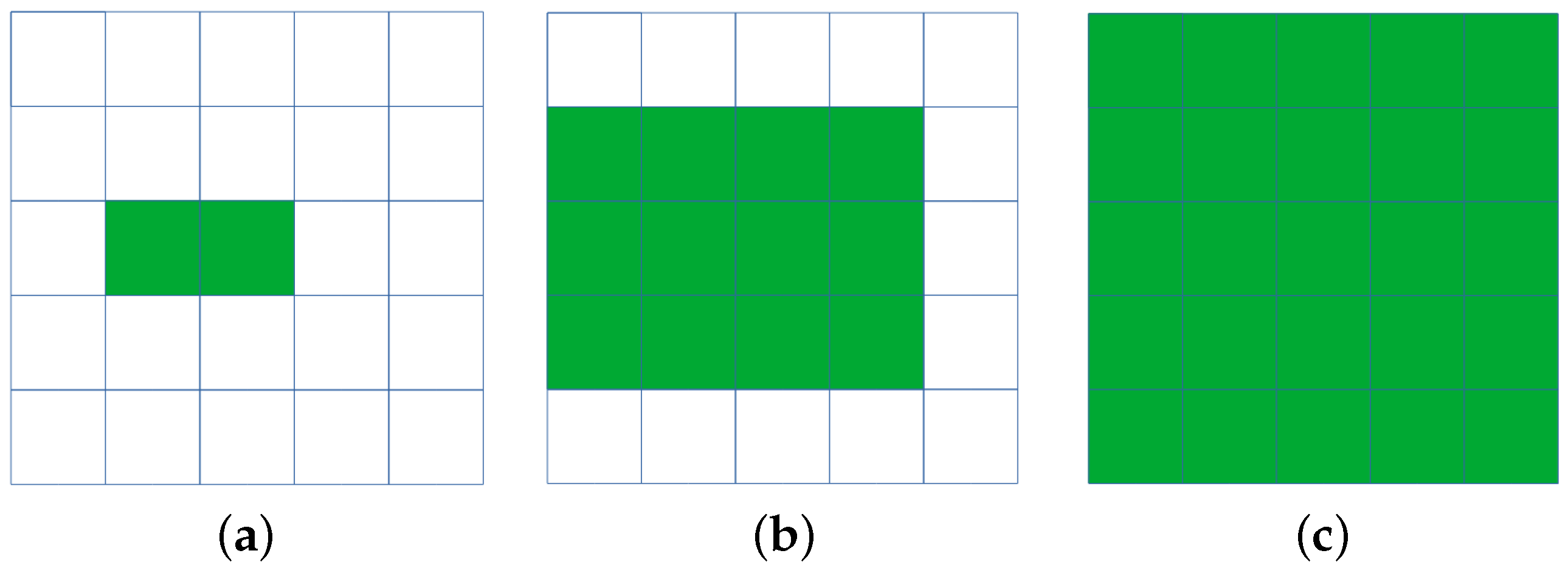
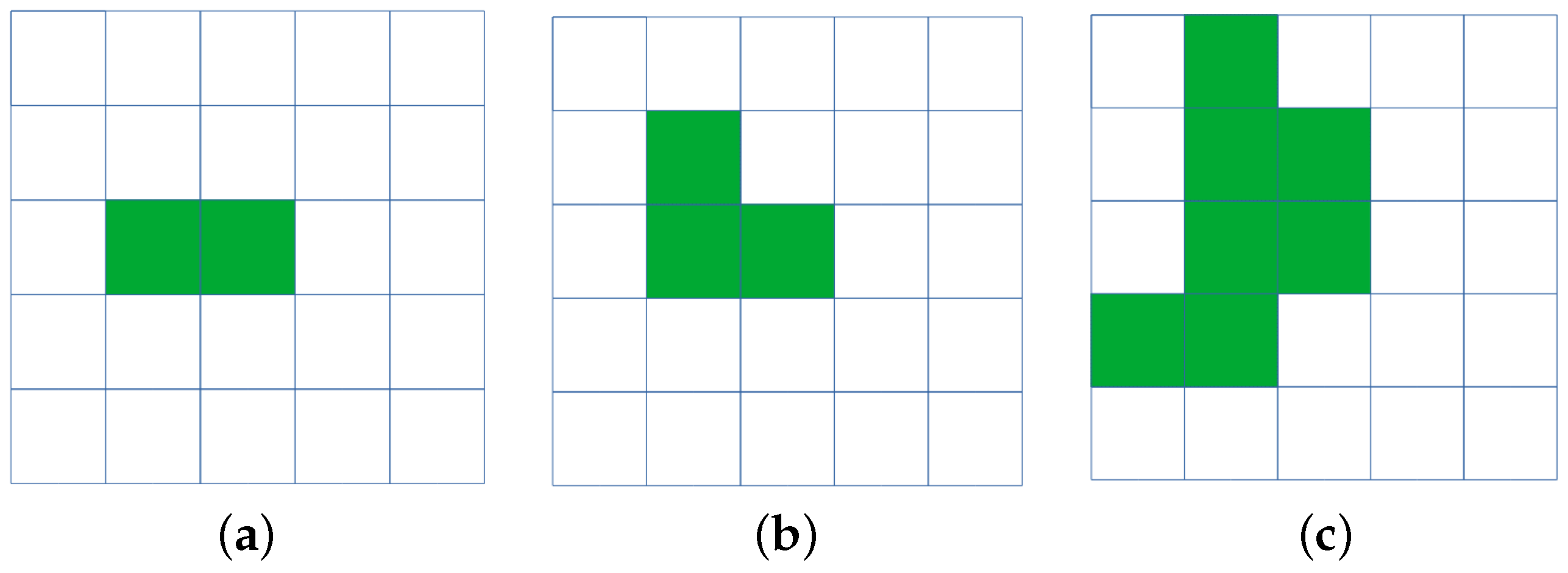
Pertinent and non-pertinent CTUs are defined at the frame where object detection is performed. Afterwards, the object in a pertinent CTU might move to neighboring CTUs. The case where it moves to the CTU of a skipped tile is captured in the Decision Module through variance detection. Nevertheless, a mechanism is needed to tackle the case whereby it moves on a neighboring CTU belonging to a non-skipped tile. We experiment with two approaches, namely, brute force area expansion and directional expansion. For each pertinent CTU, both approaches define a pertinent area. Initially, this area consists only of the aforementioned CTU. Every × frames (in the experiments it is equal to 2), the area is expanded by adding more CTUs. CTUs are only Eligible for addition if they belong to non-skipped tiles.

In the brute force approach, the expansion consists of adding all adjacent to the pertinent area CTUs, see Figure 7 for an example. In the directional approach, adjacent CTUs are added according to the variance technique used in the Decision Module. Namely, luma variance of the candidate CTU is calculated for the current and the previous frame and their absolute difference is checked against a threshold. The same threshold value used in the Decision Module is used here too. Figure 8 provides an example of the directional method. Notice that in all cases, the pertinent area can only be expanded, or remain the same, meaning that once a CTU is marked as pertinent, it remains so until the next object detection invocation. This is a rather conservative decision, aiming at minimizing potentially negative impacts on quality.

5. Experimental Results

In this section, we present the experimental evaluation. Section 5.1 describes the experimental setup. Encoding performance and accuracy against the default setting scenario are measured in Section 5.2. Section 5.3 evaluates the effects of the Decision and Tile Partitioning Module while Section 5.4 provides results concerning the algorithm’s tunable parameters. A comparison with existing work is discussed in Section 5.5. Finally, Section 5.6 summarizes our key findings.

5.1. Experimental Setup

Experiments were conducted in an Ubuntu 22.04 machine, equipped with a 4-core AMD Ryzen 5 2500G CPUrunning at 3.6 GHz, 16 GB of RAM, and a 6 GB NVIDIA Geforce RTX 3050 graphics card. For video coding purposes, we focused on the VVC standard. Specifically, we used the VVenC encoder [9], which is a lightweight version (with optimizations targeting real-time applications), of the reference software for VVC, i.e., the VVC Test model (VTM) encoder [37]. Specifically, we employ the LowDelay-Fast configuration of the encoder, with fast motion search enabled, CTU size of 64 × 64 pixels, GOP size of 8 and a GOP structure involving only B frames, except for the first frame of the sequence which is an I-frame. We also enabled the Quantization Parameter Adaptation option, which allows us to define different QPs for each CTU. The base QP value was set to 32. Finally, we selected a tile grid of 3 × 3.

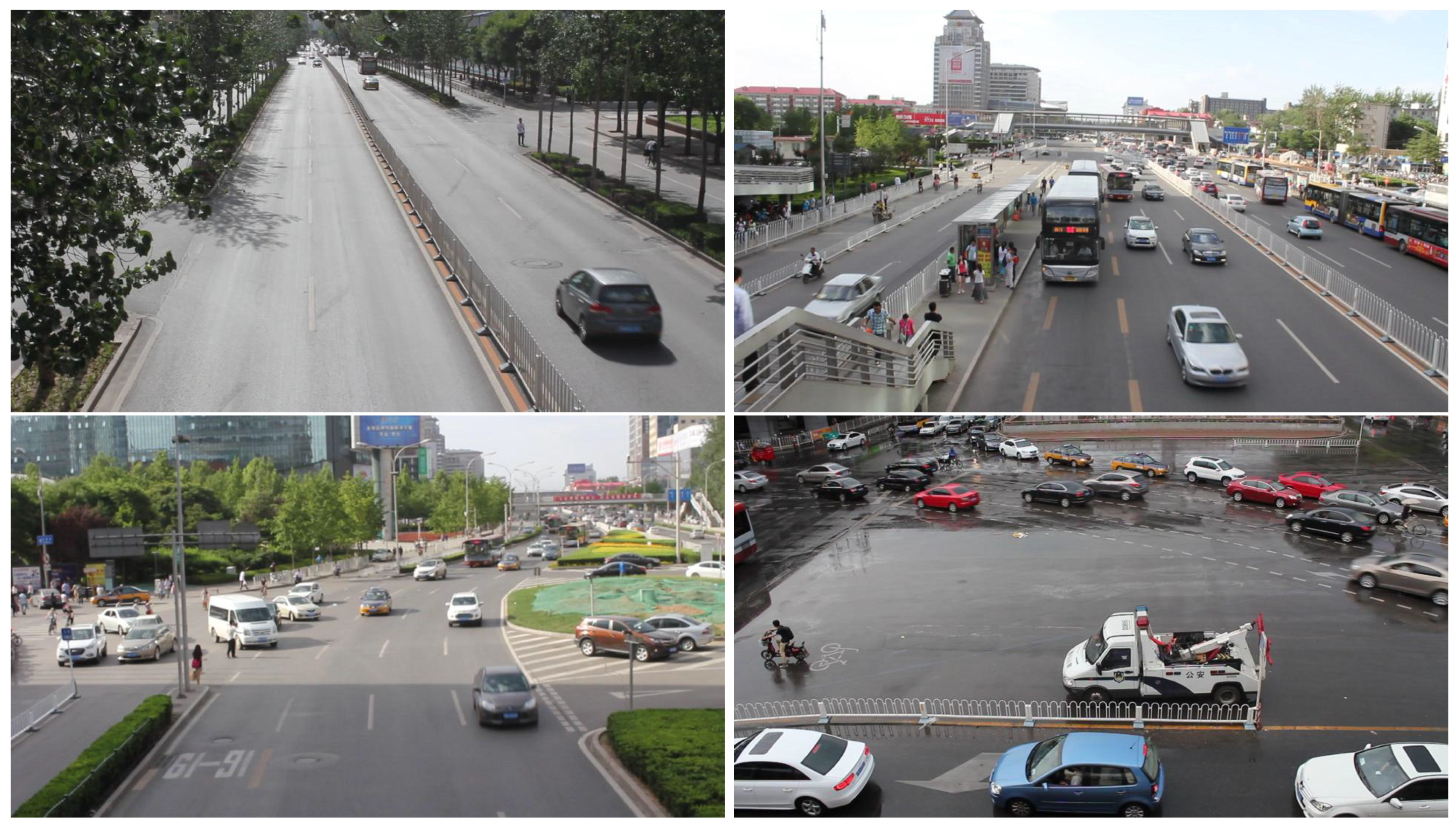
Our scheme was evaluated using the UA-DETRAC dataset [11]. This dataset consists of traffic surveillance video sequences in 960 × 540 resolution, including recordings of cameras located in intersections, highways, town centres, etc. In particular, experiments were performed with the 40 video sequences marked for evaluation by the dataset creators. In these sequences, duration ranges between 380 and 2100 frames. In Figure 9, we showcase example frames of the dataset used. Unless otherwise stated, all results depict the average performance over all 40 sequences.

For the purposes of object detection, we employ Mask R-CNN [10]. Recall that in our algorithm, whenever the object detection module is invoked, the resulting tile partition will contain tiles with no objects (if possible) that will be skipped, as well as tiles that contain objects and will be encoded. Yet the module is not invoked upon every frame; therefore, an object might move from a tile marked for encoding to a tile marked as skipped. Furthermore, new objects might appear in skipped tile areas.

In order to quantify these effects, we use various accuracy metrics. Specifically, the basic metric (accuracy) concerns the percentage of objects captured partially or fully within tiles that will be encoded. Other used metrics include: the percentage of objects caught fully within the encoded tiles (Full Object Accuracy), the percentage of the total object area that overlaps with encoded tiles (Area Overlap), and the percentage of the total object area of objects encoded partially, that overlaps with encoded tiles (Area Overlap of Partial Hit). Calculating all the aforementioned accuracy metrics requires object detection to be performed in every frame, so as to obtain the ground truth and compare it against the decisions by our algorithm. To achieve this, intentionally, we employ a different network compared to the one in the algorithm, namely, the You Only Look Once for Panopticon Driving Perception (YOLOP) DNN [17]. Notice that the two different networks might differ in object detection decisions, i.e., one might recognize an object and another might not. Accuracy metrics were calculated by taking into account only YOLOP results, which represents the most adverse scenario for our algorithm.

5.2. Encoding Performance and Accuracy

Firstly, we evaluate the performance of our algorithm against the default LowDelay-Fast encoding scenario of VVenC with a uniform 3 × 3 tile partition that remains static. All encoding parameters, i.e., GOP structure, QP value, etc., were the same as the ones described for the algorithm in Section 5.1, with the obvious exception that no QP offset was defined since it is only used by our algorithm. Notice, that compared to our algorithm, the default mode performs no object detection, thus encoding all tiles.

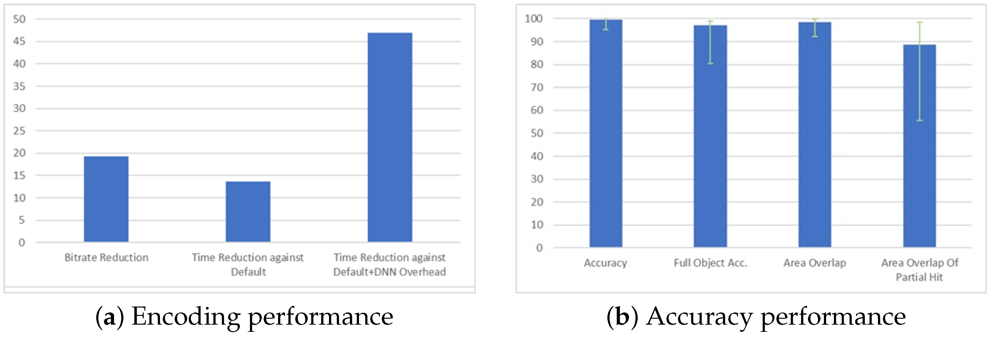
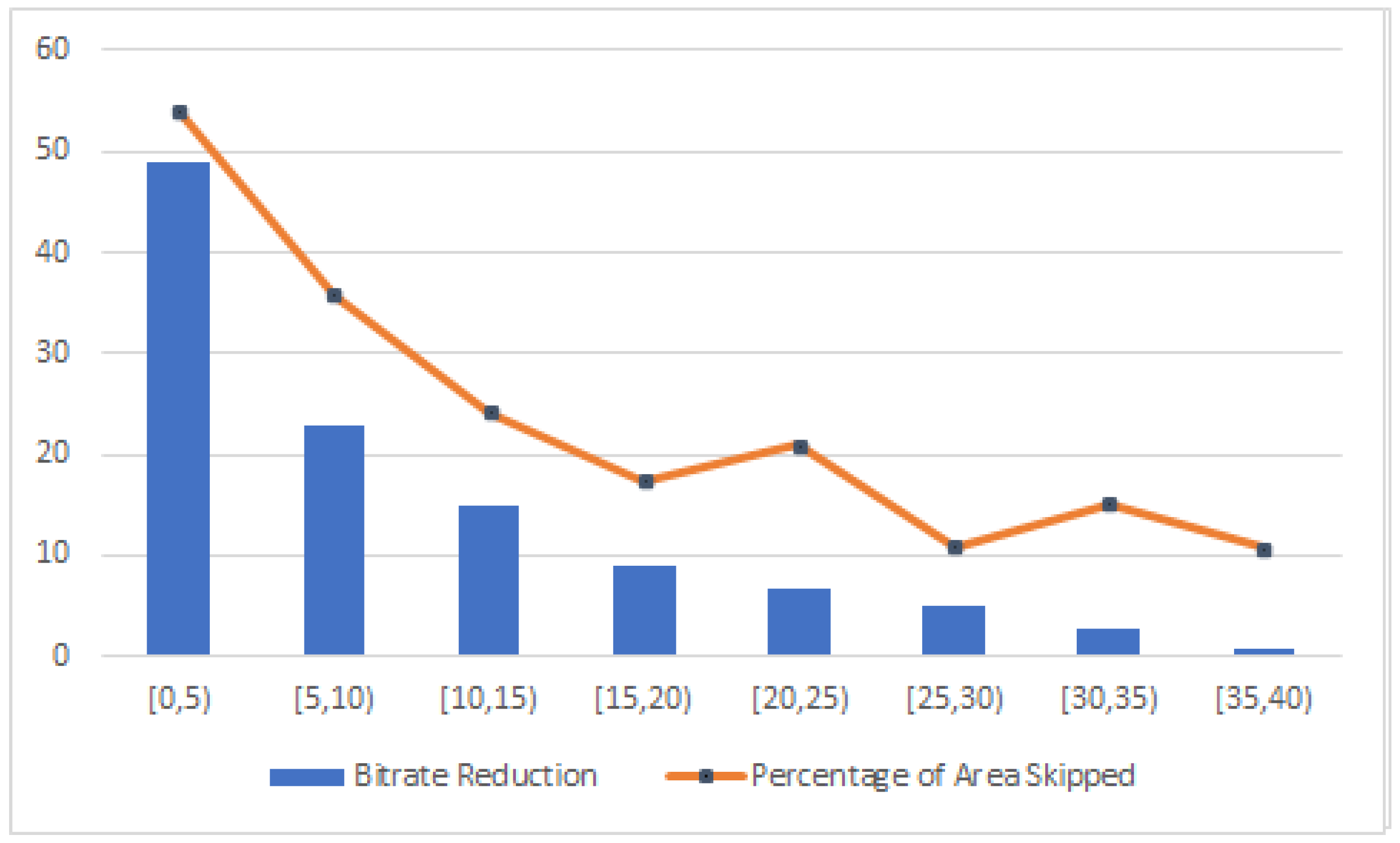
In Figure 10a, we present bitrate and running time performance. Results demonstrate that our algorithm achieves, on average, substantial reductions of 19% in bitrate and 13% in running time, with a 45% reduction in encoding time if we include the invocation of the DNN module in the default configuration. Concerning bitrate, this is largely the outcome of skipping tiles containing no objects. To further investigate this, in Figure 11, we plot the correlation between bitrate reduction and the average area percentage of the frame that is skipped. We can see a strong correlation between bitrate savings and the area that non-pertinent tiles occupy in the videos, which in Pearson correlation terms is 0.85. Furthermore, we can observe that in the majority of videos, the area occupied by objects is large. As a matter of fact, about 75% of videos have an average area percentage of non-pertinent tiles (that would be skipped) of less than 30%. Concerning time performance, both skipped tiles and QP offset contribute to the reduction. Although substantial, the 13% running time reduction shown in Figure 10a might not appear impressive at first. However, by recalling that the default encoding mode we compare against performs no object detection while our algorithm does, the merits of our approach in running time terms are better highlighted. We delve more into it in subsequent experiments.

Figure 10b illustrates results in accuracy terms, where for each metric, the average value is plotted along with the maximum and minimum values observed. As it pertains to the detection of objects, we report accuracy of over 99% in items caught partially or fully within encoded tiles by our implementation (accuracy). It is important to note that the slight degree of inaccuracy of less than 1% is largely attributed to the fact that the object detection module, if triggered, runs at the starting frame of the subsequent GOP, thus introducing a delay of up to seven frames between triggering and invocation. As shown later in the experiments, this was a necessary compromise in order to achieve good trade-off between running time and accuracy.

Regarding full object capturing and encoding, our algorithm’s accuracy is in the range of 97% (Full Object Accuracy). Comparing the total area (measured in CTUs) of objects that were detected and encoded in tiles against the total area of objects in the frames yields an overlap of roughly 98% for our algorithm (Area Overlap). Viewing this result in a reverse manner, it means that only 2% of the object information is missed by the algorithm. Our maximum value for Area Overlap reaches 98%, while our algorithm achieves a lower bound of accuracy at more than 80%. Lastly, we measured the percentage (in area terms) of partially detected objects that were actually captured and encoded (Area Overlap of Partial Hit). It turned out that more than 88% of the area of such objects was actually captured and encoded, which means that for the majority of partial hits, essential information for identification or restructuring is encoded by the algorithm.

5.3. Effects of Decision and Tile Partitioning Modules

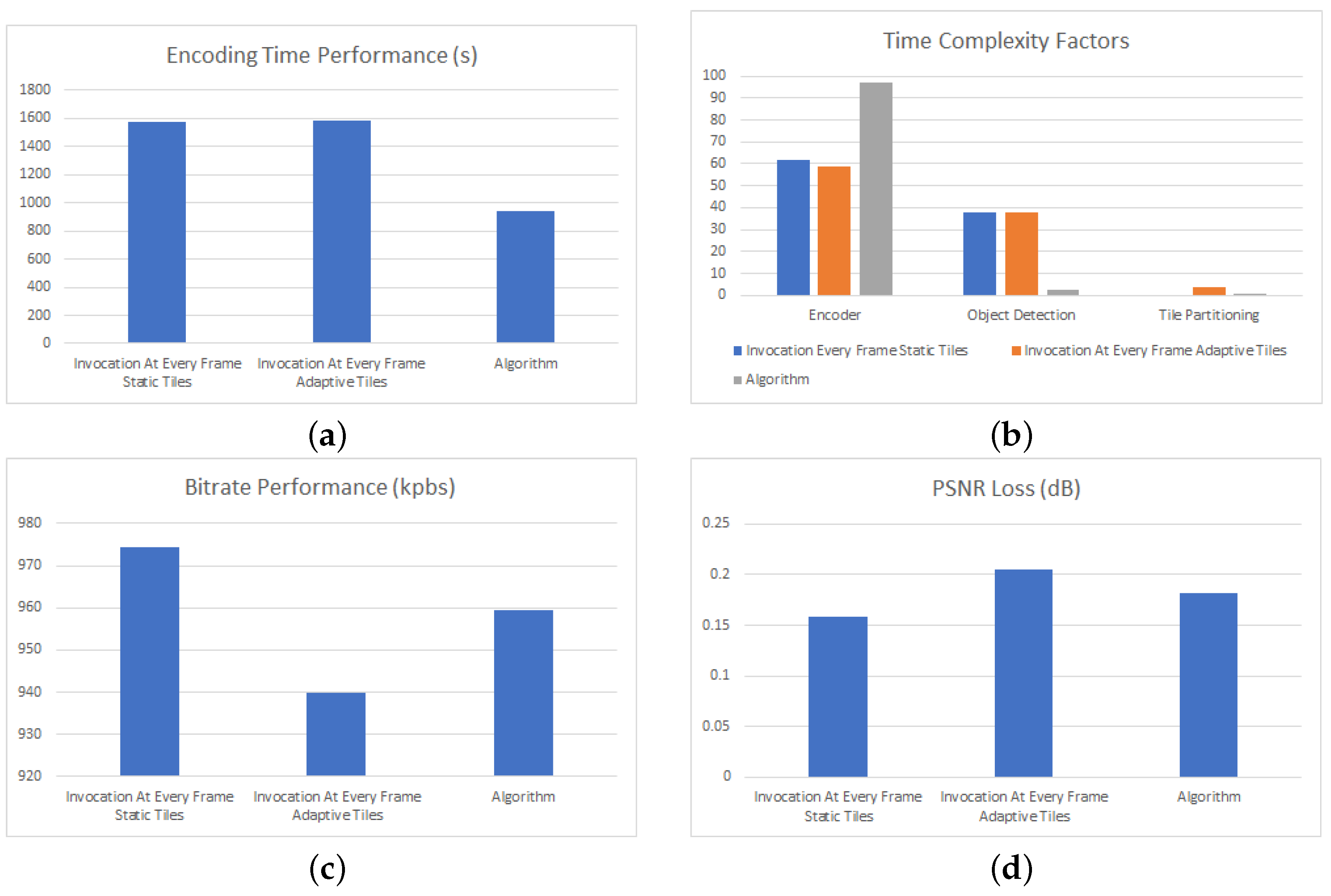
Next, we proceed by evaluating the effects that the decision and tile partitioning modules have on our algorithm’s performance. As a yardstick for comparison, we consider a simple decision scheme whereby object invocation is performed on every frame and proceed by testing against two variations of it, one that uses the same tile partitioning module as our algorithm and another one that uses a uniform tile partitioning that remains static. In Figure 12, we depict the results in terms of running time, bitrate, and quality performance. Since all videos in the dataset had the same resolution, we recorded the average running time per sequence, weighted to the number of frames at each sequence. In Figure 12a, we show running time results, while in Figure 12b, we provide a breakdown of time complexity into the time spent for encoding, object detection, and tile partitioning (shown as percentages of the total time). Clearly, our algorithm outperforms considerably in comparison with the two alternatives, accounting for roughly 40% less running time, see Figure 12a. Delving on the causes of such performance, we can observe from Figure 12b that invoking the object detection module at every frame accounts for roughly 38% of the total processing time, whereas in our algorithm, it is less than 3%. Comparing the two alternatives of invocation at every frame, we can notice that they exhibit equivalent time performance, with some minimal differences occurring due to the fact that one calls the tile partitioning module upon every frame, while the other never does so.

In Figure 12c, we illustrate bitrate performance. As expected, running object detection and tile partitioning on every frame yields more opportunities for defining tiles that can be skipped; thus, it accounts for the smallest bitrate. On the other hand, invoking continuous object detection, if accompanied by a fixed static tile partition, results in the worst performance. The result can be explained by considering that in static tile partitioning, skipped tiles can only occur if, by chance, they contain no objects, whereas in adaptive tile partitioning the tile grid changes so as to create tiles with no objects. Viewing this result from another perspective, it provides further evidence of the merits of the tile partitioning module used by the algorithm. Our algorithm falls in between the two alternatives, which can be explained by the fact that it accounts for less object detection and tile partitioning invocations compared to the upon every frame strategy. However, the bitrate difference is rather at the small end, accounting for a roughly 2% increase. Finally, in Figure 12d, we record quality performance, in terms of Peak Signal to Noise Ratio (PSNR) loss for objects. Specifically, for each method, we measure the PSNR of the encoded objects and compare it with the one in the default encoding settings used in Section 5.2. Once more, the two variations of the invocation at every frame approach account for the best and worst performance, with our algorithm falling in between, while static tile partitioning accounts for the smallest loss. This is rather expected since static tiles retain dependencies for inter- and intra-prediction to a higher degree compared to adaptive ones. However, regardless of the algorithm, the loss shown is very small, not exceeding 0.2 dB.

5.4. Parameter Calibration

Following, we evaluated the effects of certain parameters in our algorithm, namely the QP selection strategies and the threshold in CTU variance. We begin by evaluating the different strategies for QP modification discussed in Section 4.4, i.e., brute force and directional, and compare them against a scheme that accounts for no modification, i.e., it retains a QP value of 32 for all CTUs in an encoded tile. Figure 13 presents the results. In terms of bitrate (Figure 13a), directional expansion achieves the best performance, clearly outperforming the other two, while the no modification approach is the worst option. This is expected, since both brute force and directional expansion methods encode portions of the tile (the ones with no objects) using a higher QP value. Among these two methods, the directional method less eagerly expands the pertinent area around an object (an area that should be encoded with a QP value of 32), compared to brute force, hence the differences. Having more CTUs encoded at a higher QP level also aids in encoding time, whereby again the directional method outperforms the other two, as shown in Figure 13b. As expected, the downside of higher QP values is in terms of quality. In Figure 13c, we illustrate the quality loss. Specifically, for each method, we measure the PSNR of the encoded objects and compare it with the one in the default encoding setting used in Section 5.2. The directional method accounts for the largest PSNR loss, followed by the brute force method, followed by the no modification approach. Notice, that although both the no modification method and the default encoding setting use QP = 32 throughout a tile, the first still accounts for a negligible quality degradation of roughly 0.08 dB. This drop in quality, albeit insignificant, can be explained by tile adaptation that might result in the absence of suitable intra-mode reference pixels and collocated blocks in previous frames. Given the fact that the higher PSNR loss recorded by the directional method is very small, roughly 0.18 dB, and that object detection accuracy is not affected by any particular mode selection (network invocation and tile-grid formation are not influenced by the encoding process), the advantages of the directional method, in terms of bitrate and processing time, offer a valid trade-off.

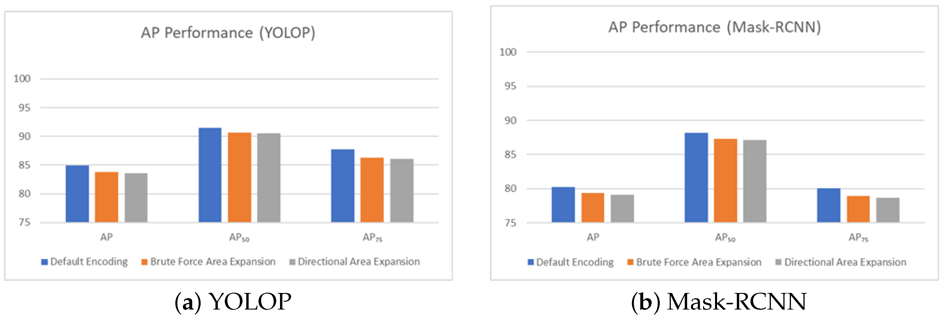
Moreover, Figure 14 provides insight in the effects of encoding and QP modification in terms of Average Precision (AP), i.e, the average Intersection Over Union (IoU) of the rectangular areas of objects detected by the DNN in the raw dataset against the collocated detected objects in decoded videos. Additionally, we calculate AP₅₀ and AP₇₅, which essentially applies thresholding to the IoU value. If the IoU value is lower than the bound specified in the subscript the object is considered missed, while equal or greater IoU values to the threshold signify detection of the objects. As a consequence, AP₅₀ and AP₇₅ are more lax criteria for the success of detection. Comparing the raw image data to the decoded video output, we observe little difference in AP between the default encoding and our algorithm for each different QP modification approach. In detail, the AP values observed are 85% for YOLOP and 80% for Mask R-CNN. In both cases, the difference between default encoding and the Brute Force Expansion approach for QP modification is just a little over than 1%, while the Directional Area Expansion achieves lower AP to the Brute Force approach by about 0.2%. These effects are also mirrored in the cases of the more lax thresholded APs of AP₅₀ and AP₇₅.

Recall from Section 4.2 that the decision of whether object detection should be performed or not is based on comparing CTU variance against a threshold. The same threshold is used also for the expansion phase in the directional mode previously discussed. In Figure 15, we evaluate the effects of the threshold in bitrate, processing time, and accuracy terms, as its value rises from 10 to 40. As shown in Figure 15a, threshold values have a mixed effect in bitrate, with the high value of 40 achieving the best results and the medium value of 20 the worst ones. This behaviour is rather the outcome of three effects that take place when threshold increases. On the Decision Module, object detection is triggered less frequently; thus, tile grid remains unchanged for more frames. This in terms leads to two effects with opposite outcomes on bitrate. The first one is that the encoding of CTUs located in tile boundaries can be conducted more efficiently since tile boundaries remain the same in reference frames, thus resulting in better bitrate. The second one is that the opportunity of redefining tile grid and subsequently optimizing tile areas to be skipped (saving bitrate) is restricted. As far as its effects on the directional mode is concerned, a higher threshold leads to less expansion; thus, more CTUs will be encoded at a higher QP and bitrate will be reduced. The cumulative effects of the above factors are depicted in Figure 15a, explaining the lack of a clear trend. In any case, the differences in bitrate between the worst and the best performer were less than 2%.

Concerning processing time, shown in Figure 15b, a clear trend exists with higher threshold values resulting in more time savings compared to lower ones. This can be explained since the aforementioned effects of higher threshold, i.e., fewer object detection invocations, less adaptive tile grids, and more CTUs encoded at high QP, all contribute to reducing processing time, resulting in a performance margin of roughly 4% between high and low threshold values. However, this performance improvement comes at the price of reduced accuracy as shown in Figure 15c, which shows that threshold increase has a detrimental effect. This is expected due to the reduced number of object detection invocations as the threshold rises. Notice that in terms of partial object hits (accuracy), performance drops from roughly 99% when the threshold is 10, to 98.5% for a threshold value of 40. The performance difference further increases as far as Full Object Accuracy is concerned with a gap of roughly 3%, while it becomes very large regarding the Area Overlap of Partial Hits, whereby a downgrade of roughly 13% is recorded. Given that accuracy is of utmost importance, the overall results of Figure 15 justify the reason why we selected the rather small threshold value of 10 in the basic configuration of our algorithm (discussed in Section 5.1).

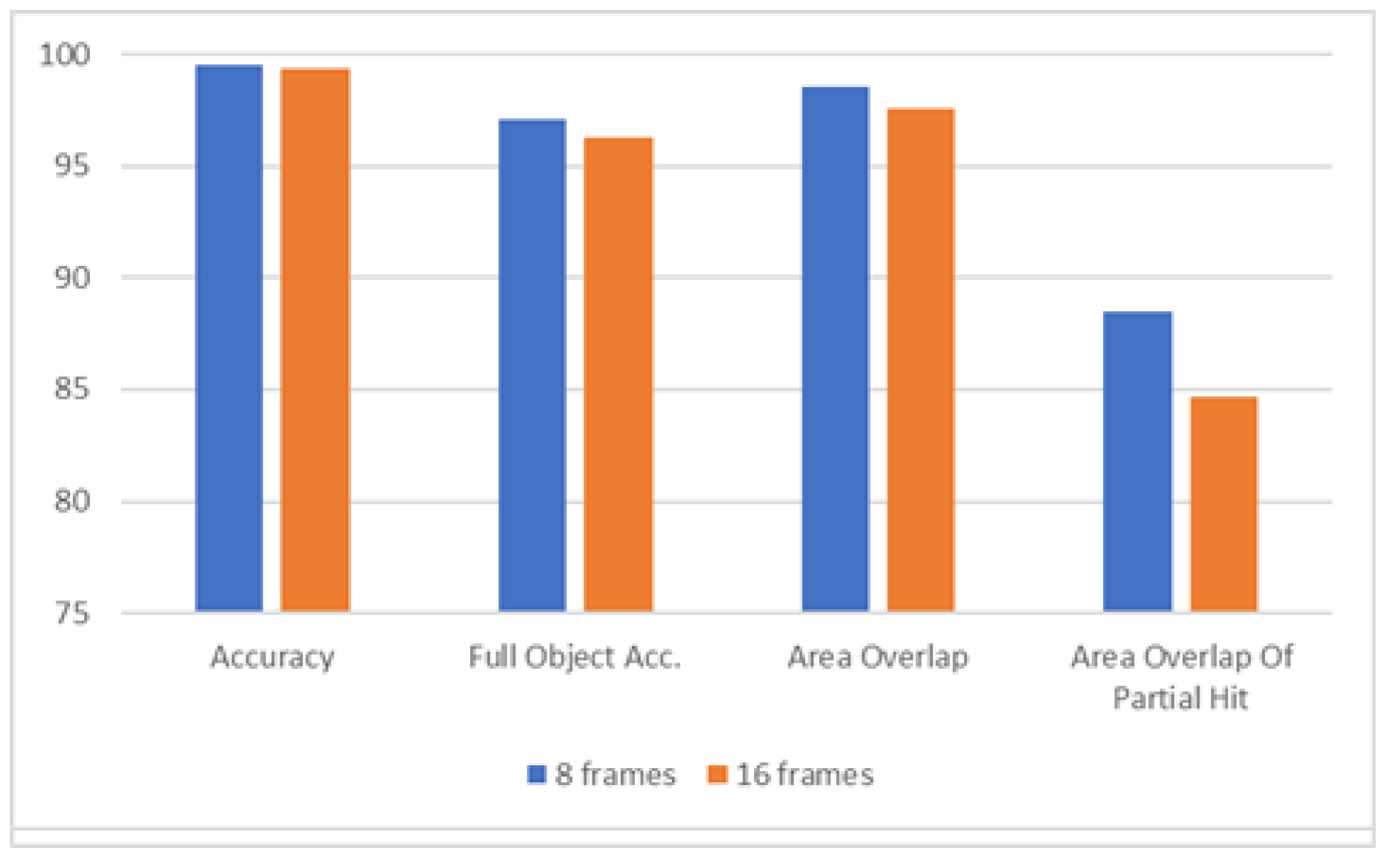
Finally, in Figure 16, we summarize the trade-off between accuracy and invocation period by plotting our accuracy metrics for different invocation windows. As expected, we can observe that the latency of the invocation affects the accuracy performance of our algorithm, albeit marginally. As latency increases from 8 frames to 16 frames, there is a dropoff for all the accuracy metrics. Namely, the dropoff is observed to be 0.2% for accuracy, 0.7% for Full Object Accuracy, 1% for Area Overlap, and about 4% for Area Overlap of Partial Hit.

5.5. Comparison with Other Works

As discussed in the related work (Section 3), we are aware of the most similar scope to the algorithm of this paper, which is TileClipper presented in [35]. Although a direct comparison is not possible, since the implementation of TileClipper concerned HEVC, in

Table 1. Comparison with [29,35].

	Bitrate Reduction (%)	Accuracy (%)
Algorithm	20.70	99.26
TileClipper	22.06	95.48
CloudSeg	61.41	97.04

, we summarize key performance metrics as obtained by [35] for the UA-DETRAC dataset and for discussion purposes, corresponding results by our algorithm. Since results in [35] were obtained using a 4 × 4 uniform and static tile grid, for comparison reasons, we run our algorithm using a 4 × 4 tile grid. The first thing to notice is that accuracy (in partial hit terms) of our algorithm is considerably larger compared to TileClipper, 99.26% versus 95.48%. This indicates that the variance-based method for triggering object detection proposed in this paper is more advantageous compared to the bitrate based method of [35]. Furthermore, in our algorithm, whenever object detection is performed, it happens upon the whole frame, while in TileClipper, it does not. Due to lack of results in [35] concerning full object hits and Area Overlap performance, no further comparisons in these aspects could be performed. For the record, the performance achieved by our algorithm for these metrics was the following: 95.28% for Full Object Acc., 97.9% for Area Overlap, and 84% for Area Overlap Of Partial Hit. As far as processing time is concerned, our algorithm is again clearly superior. The key reason is that that TileClipper first encodes the whole frame in order to calculate bitrate and use it for tile pruning. It is also important to note that when compared to the similar default VVC encoding (used in Section 5.2), our algorithm achieves a time reduction of 11.31%. Furthermore, this is rather a lower bound in time improvement over TileClipper, as it does not take into account the extra time overhead of TileClipper for performing object detection in the tiles it selects. Lastly, we recorded the bitrate performance of the two schemes. Although results are not directly comparable since TileClipper refers to bitrate savings versus a default HEVC setting, while our algorithm versus a default VVC setting, it appears that both schemes achieve comparable savings. Overall, we can state that compared to [35], our algorithm is a clear winner with regards to accuracy and runtime, with almost equivalent performance in bitrate terms.

Additionally, while not directly inline with our scope, we also provide a comparison of our algorithm with CloudSeg [29], as reconstructed by the authors in [35]. CloudSeg manages to provide substantial savings in bitrate to the range of 61%, with its downsampling/Super Resolution strategy. However, its accuracy for the DETRAC dataset is reported at 97.04%, 2% below our algorithm using a 4 × 4 tile grid. As far as computational cost in GPU terms is concerned, CloudSeg requires GPU usage during decoding in order to derive a video back to its original resolution. As a matter of fact, TileClipper’s GPU usage, whose server side contains only object detection, is reported in [35] to be much lower than CloudSeg’s. With our approach, the GPU usage only occurs during encoding, and thus, no additional computational cost is incurred during the decoding process. The aforementioned remark, coupled with the higher accuracy that our algorithm provides, makes our approach a more suitable candidate in terms of scalability.

5.6. Discussion

Here, we summarize the key findings of the experimental evaluation:

• Compared to an equivalent scheme, whereby object detection is performed on every frame, our algorithm managed to reduce running time by roughly 40% (Figure 12a), while maintaining 99% accuracy in partial hits (Figure 10). This highlights the merits of one of our contributions, i.e., the Decision Module proposed in this paper, which only sparingly invokes the object detection DNN.
• The adaptive tile partitioning method proposed in this paper was shown to lead to more bitrate savings compared to static option (by another 3.5%), even in the case where the Decision Module was bypassed (Figure 12c). Furthermore, it incurred negligible runtime and quality overhead (Figure 12a,d).
• Using higher QP to encode non-pertinent tiles was shown to bear merits. Specifically, using the directional expansion method, further bitrate and running time savings of more than 4.5% and 3.5%, respectively, were achieved against a simple strategy that did not vary QP (Figure 13a,b). Moreover, these reductions came at a tiny overhead in encoded object quality (Figure 13c).
• Comparison of our algorithm against an equivalent default encoding setting that performs no object detection (Figure 10) confirmed our motivation. It was shown that, cumulatively, our key contributions, i.e., variance-based DNN invocation (Decision Module), adaptive tile partitioning to maximize skipped area, and different QP levels for pertinent and non-pertinent tiles, resulted in 19% bitrate reduction and 13% time reduction, despite the fact that the adversary incurred zero DNN overhead. Even more encouraging is the fact that the bitrate and time benefits come together with a good performance in accuracy terms, roughly 99% and 97% in terms of partial and full accuracy object hits.
• The merits of our algorithm were further highlighted when comparing its performance against related work of the same scope, i.e., ref. [35] (Table 1). Our algorithm managed to maintain rather equivalent bitrate performance, while incurring at least 11% processing time reduction and an additional 4% in accuracy.

6. Conclusions

In this paper, we tackled the problem of improving processing time and bitrate in video surveillance streams with object detection. Given the fact that object detection might prove costly time-wise, we developed an algorithm that takes advantage of luma variances in order to invoke the relevant DNN sparingly, i.e., when it is estimated that new objects have appeared. Once objects have been defined, adaptive tile partitioning takes place with the aim of maximizing tile areas containing no objects. Such tiles can be skipped during encoding since they only carry scenery information, which remains largely unchanged. The proposed algorithm also includes the option of encoding the areas of a tile containing objects at a higher quality level compared to the rest. At the same time, it predicts possible object movement inside the tile in order to judiciously expand the pertinent area that will be encoded at a higher quality level. Cumulatively, the aforementioned optimizations resulted in our algorithm being able to achieve (for the case of VVC) significant bitrate and running time reductions, while maintain high detection accuracy and high quality for encoded objects. The comparison against related work further highlighted the merits of our approach.

References

1. Priks, M. The Effects of Surveillance Cameras on Crime: Evidence from the Stockholm Subway. Econ. J. 2015, 125, F289–F305. [Google Scholar] [CrossRef]
2. Wiegand, T.; Sullivan, G.J.; Bjontegaard, G.; Luthra, A. Overview of the H.264/AVC video coding standard. IEEE Trans. Circuits Syst. Video Technol. 2003, 13, 560–576. [Google Scholar] [CrossRef]
3. Sullivan, G.J.; Ohm, J.R.; Han, W.J.; Wiegand, T. Overview of the High Efficiency Video Coding (HEVC) Standard. IEEE Trans. Circuits Syst. Video Technol. 2012, 22, 1649–1668. [Google Scholar] [CrossRef]
4. Bross, B.; Wang, Y.K.; Ye, Y.; Liu, S.; Chen, J.; Sullivan, G.J.; Ohm, J.R. Overview of the Versatile Video Coding (VVC) Standard and its Applications. IEEE Trans. Circuits Syst. Video Technol. 2021, 31, 3736–3764. [Google Scholar] [CrossRef]
5. Siqueira, I.; Correa, G.; Grellert, M. Rate-Distortion and Complexity Comparison of HEVC and VVC Video Encoders. In Proceedings of the Latin American Symposium of Circuits and Systems, San Jose, Costa Rica, 25–28 February 2020; pp. 1–4. [Google Scholar] [CrossRef]
6. Amestoy, T.; Hamidouche, W.; Bergeron, C. Quality-Driven Dynamic VVC Frame Partitioning for Efficient Parallel Processing. In Proceedings of the IEEE International Conference on Image Processing, Abu Dhabi, United Arab Emirates, 25–28 October 2020; pp. 3129–3133. [Google Scholar] [CrossRef]
7. George, V.; Brandenburg, J.; Hege, G.; Hinz, T.; Wieckowski, A.; Bross, B.; Schierl, T.; Marpe, D. Inter-Frame Parallelization in an Open Optimized VVC Encoder. In Proceedings of the 15th ACM Multimedia Systems Conference, Bari, Italy, 15–18 April 2024; pp. 202–209. [Google Scholar] [CrossRef]
8. Dong, X.; Shen, L.; Yu, M.; Yang, H. Fast Intra Mode Decision Algorithm for Versatile Video Coding. IEEE Trans. Multimed. 2022, 24, 400–414. [Google Scholar] [CrossRef]
9. Wieckowski, A.; Brandenburg, J.; Hinz, T.; Bartnik, C.; George, V.; Hege, G.; Helmrich, C.; Henkel, A.; Lehmann, C.; Stoffers, C.; et al. VVenC: An Open And Optimized VVC Encoder Implementation. In Proceedings of the IEEE International Conference on Multimedia & Expo Workshops, Shenzhen, China, 5–9 July 2021; pp. 1–2. [Google Scholar] [CrossRef]
10. He, K.; Gkioxari, G.; Dollár, P.; Girshick, R. Mask R-CNN. In Proceedings of the IEEE International Conference on Computer Vision, Venice, Italy, 22–29 October 2017. [Google Scholar] [CrossRef]
11. Wen, L.; Du, D.; Cai, Z.; Lei, L.; Chang, M.; Qi, H.; Lim, J.; Yang, M.; Lyu, S. UA-DETRAC: A New Benchmark and Protocol for Multi-Object Detection and Tracking. Comput. Vis. Image Underst. 2020, 193, 102907. [Google Scholar] [CrossRef]
12. Han, J.; Li, B.; Mukherjee, D.; Chiang, C.H.; Grange, A.; Chen, C.; Su, H.; Parker, S.; Deng, S.; Joshi, U.; et al. A Technical Overview of AV1. Proc. IEEE 2021, 109, 1435–1462. [Google Scholar] [CrossRef]
13. Dalal, N.; Triggs, B. Histograms of oriented gradients for human detection. In Proceedings of the Computer Society Conference on Computer Vision and Pattern Recognition, San Diego, CA, USA, 20–25 June 2005; IEEE: Piscataway, NJ, USA, 2005; Volume 1, pp. 886–893. [Google Scholar] [CrossRef]
14. Viola, P.; Jones, M. Rapid object detection using a boosted cascade of simple features. In Proceedings of the IEEE Computer Society Conference on Computer Vision and Pattern Recognition,Kauai, HI, USA, 8–14 December 2001; IEEE: Piscataway, NJ, USA, 2001; Volume 1. [Google Scholar] [CrossRef]
15. Zhu, X.; Dai, J.; Yuan, L.; Wei, Y. Towards High Performance Video Object Detection. In Proceedings of the IEEE Conference on Computer Vision and Pattern Recognition, Salt Lake City, UT, USA, 18–23 June 2018; pp. 7210–7218. [Google Scholar] [CrossRef]
16. Han, W.; Khorrami, P.; Paine, T.L.; Ramachandran, P.; Babaeizadeh, M.; Shi, H.; Li, J.; Yan, S.; Huang, T.S. Seq-NMS for Video Object Detection. arXiv 2016, arXiv:1602.08465. [Google Scholar] [CrossRef]
17. Wu, D.; Liao, M.; Zhang, W.; Wang, X.; Bai, X.; Cheng, W.; Liu, W. YOLOP: You Only Look Once for Panoptic Driving Perception. Mach. Intell. Res. 2022, 19, 550–562. [Google Scholar] [CrossRef]
18. Ren, S.; He, K.; Girshick, R.; Sun, J. Faster R-CNN: Towards Real-Time Object Detection with Region Proposal Networks. IEEE Trans. Pattern Anal. Mach. Intell. 2017, 39, 1137–1149. [Google Scholar] [CrossRef] [PubMed]
19. Cai, F.; Qu, Z.; Xia, S.; Wang, S. A method of object detection with attention mechanism and C2f_DCNv2 for complex traffic scenes. Expert Syst. Appl. 2025, 267, 126141. [Google Scholar] [CrossRef]
20. Meng, B.; Zhang, L.; Jin, F.; Yang, L.; Cheng, H.; Wang, Q. Abnormal Events Detection Using Deep Networks for Video Surveillance. In Proceedings of the International Conference on Cognitive Systems and Signal Processing, Beijing, China, 19–23 November 2016; pp. 197–204. [Google Scholar] [CrossRef]
21. Venkatrayappa, D. Abnormal Event Detection In Videos Using Deep Embedding. arXiv 2024, arXiv:2409.09804. [Google Scholar] [CrossRef]
22. Panagou, N.; Belememis, P.; Koziri, M. Image Segmentation Methods for Subpicture Partitioning in the VVC Video Encoder. Electronics 2022, 11, 2070. [Google Scholar] [CrossRef]
23. Belememis, P.; Panagou, N.; Koziri, M.; Loukopoulos, T. Review and comparative analysis of parallel video encoding techniques for VVC. In Proceedings of the SPIE Applications of Digital Image Processing XLIII, Sand Diego, CA, USA, 24 August–4 September 2020; SPIE: Bellingham, WA, USA, 2020; Volume 11510. [Google Scholar] [CrossRef]
24. Tang, N.; Cao, J.; Liang, F.; Wang, J.; Liu, H.; Wang, X.; Du, X. Fast CTU Partition Decision Algorithm for VVC Intra and Inter Coding. In Proceedings of the IEEE Asia Pacific Conference on Circuits and Systems, Bangkok, Thailand, 11–14 November 2019; pp. 361–364. [Google Scholar] [CrossRef]
25. Fischer, K.; Fleckenstein, F.; Herglotz, C.; Kaup, A. Saliency-Driven Versatile Video Coding for Neural Object Detection. In Proceedings of the International Conference on Acoustics, Speech, and Signal Processing, Toronto, ON, Canada, 6–11 June 2021; pp. 1505–1509. [Google Scholar] [CrossRef]
26. Lee, Y.; Kim, S.; Yoon, K.; Lim, H.; Kwak, S.; Choo, H.G. Machine-Attention-based Video Coding for Machines. In Proceedings of the IEEE International Conference on Image Processing, Kuala Lumpur, Malaysia, 8–11 October 2023; pp. 2700–2704. [Google Scholar] [CrossRef]
27. Kong, L.; Dal, R. Efficient Video Encoding for Automatic Video Analysis in Distributed Wireless Surveillance Systems. ACM Trans. Multimed. Comput. Commun. Appl. 2018, 14, 1–24. [Google Scholar] [CrossRef]
28. Kim, H.; Khudoyberdiev, A.; Garnaik, S.; Bhattacharya, A.; Ryoo, J. CLOUD-CODEC: A New Way of Storing Traffic Camera Footage at Scale. ACM Trans. Multimed. Comput. Commun. Appl. 2025, 21, 1–28. [Google Scholar] [CrossRef]
29. Wang, Y.; Wang, W.; Zhang, J.; Jiang, J.; Chen, K. Bridging the Edge-Cloud Barrier for Real-time Advanced Vision Analytics. In Proceedings of the 11th USENIX Workshop on Hot Topics in Cloud Computing, Renton, WA, USA, 8 July 2019. [Google Scholar]
30. Chen, S.; Deng, J.; Tao, X.; Xie, X.; Tan, R.; Hong, T.; Liu, X. Bandwidth on a Budget: Real-Time Configuration for Edge Video Analysis. IEEE Trans. Comput. 2025, 75, 409–422. [Google Scholar] [CrossRef]
31. Zhang, M.; Wang, F.; Liu, J. CASVA: Configuration-Adaptive Streaming for Live Video Analytics. In Proceedings of the IEEE INFOCOM 202, London, UK, 2–5 May 2022. [Google Scholar] [CrossRef]
32. Du, K.; Pervaiz, A.; Yuan, X.; Chowdhery, A.; Zhang, Q.; Hoffmann, H.; Jiang, J. Server-Driven Video Streaming for Deep Learning Inference. In Proceedings of the Annual conference of the ACM Special Interest Group on Data Communication on the Applications, Technologies, Architectures, and Protocols for Computer Communication, Virtual Event, 10–14 August 2020. [Google Scholar] [CrossRef]
33. Guo, H.; Yao, S.; Yang, Z.; Zhou, Q.; Nahrstedt, K. CrossRoI: Cross-camera region of interest optimization for efficient real time video analytics at scale. In Proceedings of the 12th ACM Multimedia Systems Conference, Istanbul, Turkey, 28 September–1 October 2021; pp. 557–570. [Google Scholar] [CrossRef]
34. Xiao, J.; Hu, R.; Liao, L.; Chen, Y.; Wang, Z.; Xiong, Z. Knowledge-Based Coding of Objects for Multisource Surveillance Video Data. IEEE Trans. Multimed. 2016, 18, 1691–1706. [Google Scholar] [CrossRef]
35. Chaudhary, S.; Taneja, A.; Singh, A.; Roy, P.; Sikdar, S.; Maity, M.; Bhattacharya, A. TileClipper: Lightweight Selection of Regions of Interest from Videos for Traffic Surveillance. In Proceedings of the 2024 USENIX Conference on Usenix Annual Technical Conference, Santa Clara, CA, USA, 10–12 July 2024; USENIX: Berkeley, CA, USA, 2024; Volume 59, pp. 967–984. [Google Scholar]
36. Chi, C.C.; Alvarez-Mesa, M.; Juurlink, B.; Clare, G.; Henry, F.; Pateux, S.; Schierl, T. Parallel Scalability and Efficiency of HEVC Parallelization Approaches. IEEE Trans. Circuits Syst. Video Technol. 2012, 22, 1827–1838. [Google Scholar] [CrossRef]
37. VTM Software Repository. Available online: https://vcgit.hhi.fraunhofer.de/jvet/VVCSoftware_VTM (accessed on 5 November 2025).
Figure 1. CU Splitting according to VVC: (a) quad, (b) binary, and (c) tertiary.
Mathematics 14 00368 g001
Figure 2. Intra-mode example. Reference pixels in previously encoded blocks (in gray) are combined to extrapolate the values of the current block’s pixels. The way by which the reference pixels will be combined is depicted in the form of arrows.
Mathematics 14 00368 g002
Figure 3. General architecture of our algorithm.
Mathematics 14 00368 g003
Figure 4. Example invocation. (a) The original frame and its split in CTUs (blue lines). (b) The 3 × 3 tile partitioning (green lines). Only three out of nine tiles contain objects and will be further processed.
Mathematics 14 00368 g004
Figure 5. Demonstration of our snap grid operation. In (a), the rectangular area is plotted as derived from the DNN (highlighted in blue), while in (b), the area is transformed to snap to the CTU grid.
Mathematics 14 00368 g005
Figure 6. (a) Example of our tile partitioning module. Areas that contain objects according to the DNN module are denoted with green, while blue lines denote the candidate tile rows and columns. Notice that some are not eligible due to tile size constraints. (b) Final tile partitioning derived by our scheme. Tiles that contain pertinent CTUs are shown filled in blue.
Mathematics 14 00368 g006
Figure 7. Simple area expansion of pertinent CTUs at (a) F = t, (b) F = t + x, and (c) F = t + 2x.
Mathematics 14 00368 g007
Figure 8. Directional expansion of pertinent CTUs at (a) F = t, (b) F = t + x, and (c) F = t + 2x. The QP expansion takes place only at CTUs that exceed the variance threshold.
Mathematics 14 00368 g008
Figure 9. Example video sequences of UA-DETRAC dataset.
Mathematics 14 00368 g009
Figure 10. Comparison of our algorithm with the default VVenC encoding.
Mathematics 14 00368 g010
Figure 11. Relationship between bitrate savings and area percentage occupied by non-pertinent tiles. The videos are ordered by bitrate reduction achieved in descending order and grouped in bins of five.
Mathematics 14 00368 g011
Figure 12. Effects of the decision and tile partitioning modules in: (a) time performance, (b) complexity contribution of modules, (c) bitrate and (d) quality. Invocation at every frame signifies the absence of the Decision Module, while static tiles signifies the absence of the tile partitioning module.
Mathematics 14 00368 g012
Figure 13. Effects of pertinent area expansion modes in (a) bitrate, (b) compression time, and (c) quality.
Mathematics 14 00368 g013
Figure 14. AP metrics of our algorithm for YOLOP and Mask-RCNN.
Mathematics 14 00368 g014
Figure 15. Effects of different variance thresholds in (a) bitrate, (b) compression time, and (c) accuracy.
Mathematics 14 00368 g015
Figure 16. Accuracy metrics for diferent invocation windows.
Mathematics 14 00368 g016