On the Whittaker Function Extended by the Fox–Wright Function and Its Properties

Abstract

This paper aims to obtain the ${}_{\xi }\mathsf{\Psi }_{\eta }$-extended Whittaker function and its integral representations. This function is defined by using the ${}_{\xi }\mathsf{\Psi }_{\eta }$-confluent hypergeometric function, which was recently extended in terms of the Fox–Wright function. Furthermore, we discuss properties including a transformation formula, integral transforms (Laplace–Mellin and Hankel transforms), and a differential formula. Our results provide a unified framework for several known generalizations of the Whittaker function and highlight potential applications in applied mathematics and theoretical physics.

1. Introduction and Preliminary

In this investigation, $\mathbb{N}$, $\mathbb{R}$, ${\mathbb{R}}^{+}$, $\mathbb{C}$, and ${\mathbb{Z}}_0^{-}$ represent sets of natural numbers, real numbers, positive real numbers, complex numbers, and non-positive integers, respectively. We also define ${\mathbb{N}}_0:=\{0,1,2,3,\dots \}=\mathbb{N}\cup \left\{0\right\}$ and ${\mathbb{R}}_0^{+}:={\mathbb{R}}^{+}\cup \left\{0\right\}$.

The Whittaker functions (${\mathrm{M}}_{\zeta ,\pm \rho }\left(\omega \right)$) arise as solutions to the Whittaker differential equation [1,2,3]:

$$w^{″}+\left({\displaystyle \frac{\frac{1}{4}-{\rho }^2}{{\omega }^2}}+{\displaystyle \frac{\zeta }{\omega }}-{\displaystyle \frac{1}{4}}\right)w=0,w={\mathrm{M}}_{\zeta ,\pm \rho }\left(\omega \right),$$

where $\omega =0$ is a branching point for ${\mathrm{M}}_{\zeta ,\rho }\left(\omega \right)$, and $\omega =\infty$ is an essential singularity. Two solutions given by the Whittaker functions (${\mathrm{M}}_{\zeta ,\pm \rho }\left(\omega \right)$) are defined in terms of Kummer’s confluent hypergeometric function, i.e.,

$${}_1\mathrm{F}_1[{\mathsf{\Lambda }}_2;{\mathsf{\Lambda }}_3;\omega ]=\mathsf{\Phi }({\mathsf{\Lambda }}_2;{\mathsf{\Lambda }}_3;\omega )=\sum _{n\ge 0}{\displaystyle \frac{{\left({\mathsf{\Lambda }}_2\right)}_n}{{\left({\mathsf{\Lambda }}_3\right)}_n}}{\displaystyle \frac{{\omega }^n}{n!}},{\mathsf{\Lambda }}_3\in \mathbb{C}\setminus {\mathbb{Z}}_0^{-},$$

(1)

and the ${\mathrm{M}}_{\zeta ,\rho }\left(\omega \right)$ function is specifically given by

$$\begin{gathered} {\mathrm{M}}_{\zeta ,\rho }\left(\omega \right)={\omega }^{\rho +{\displaystyle \frac{1}{2}}}{e}^{-{\displaystyle \frac{\omega }{2}}}\mathsf{\Phi }\left(\rho -\zeta +{\displaystyle \frac{1}{2}};2\rho +1;\omega \right), \\ (\zeta \in \mathbb{C},min\{\Re \left(\rho \right),\Re (\rho -\zeta )\}>-\frac{1}{2}), \end{gathered}$$

(2)

where $\Re (.)$ denotes the real part of a complex number.

These functions, identified by (2), have numerous applications in mathematical physics and engineering sciences, including fluid mechanics, atomic structure theory, and electromagnetic diffraction problems (see [3,4,5,6,7,8,9,10]). In the last several decades, numerous researchers have introduced and investigated various extensions of some well-known special functions (for details, see [2,4,5,6,7,8,9,10,11,12,13]). A recent study by Ata et al. (see [14]) presented a new representation of the beta function, analyzing its properties and exploring diverse applications in statistical sciences. Inspired by the aforementioned research, this paper introduces a novel generalization of the Whittaker function, utilizing the ${}_{\xi }\mathsf{\Psi }_{\eta }$-confluent hypergeometric function to express it in terms of the Fox–Wright function, and studies its properties, such as integral representations, a transformation formula, integral transforms, and a derivative formula.

In the sequel, we utilize the traditional beta function introduced by Leonhard Euler ($\mathrm{B}({\mathsf{\Lambda }}_1,{\mathsf{\Lambda }}_2)$) and defined as follows (see [15,16]):

$$\mathrm{B}({\mathsf{\Lambda }}_1,{\mathsf{\Lambda }}_2)={\int }_0^1{t}^{{\mathsf{\Lambda }}_1-1}{(1-t)}^{{\mathsf{\Lambda }}_2-1}\mathrm{d}t,min\{\Re \left({\mathsf{\Lambda }}_1\right),\Re \left({\mathsf{\Lambda }}_2\right)\}>0.$$

(3)

The gamma function ($\mathsf{\Gamma }\left({\mathsf{\Lambda }}_1\right)$) is defined by the convergent improper integral as follows:

$$\mathsf{\Gamma }\left({\mathsf{\Lambda }}_1\right)={\int }_0^{\infty }{t}^{{\mathsf{\Lambda }}_1-1}{e}^{-t}\mathrm{d}t,\Re \left({\mathsf{\Lambda }}_1\right)>0.$$

(4)

These two functions are interconnected through the following formula:

$$\mathrm{B}({\mathsf{\Lambda }}_1,{\mathsf{\Lambda }}_2)={\displaystyle \frac{\mathsf{\Gamma }\left({\mathsf{\Lambda }}_1\right)\mathsf{\Gamma }\left({\mathsf{\Lambda }}_2\right)}{\mathsf{\Gamma }({\mathsf{\Lambda }}_1+{\mathsf{\Lambda }}_2)}},{\mathsf{\Lambda }}_1,{\mathsf{\Lambda }}_2\in \mathbb{C}\setminus {\mathbb{Z}}_0^{-}.$$

The Pochhammer symbol (${\left({\mathsf{\Lambda }}_1\right)}_{\mathsf{\ell }}$) is defined by (see [1,15])

$$\begin{array}{c}\hfill {\left({\mathsf{\Lambda }}_1\right)}_{\mathsf{\ell }}:={\displaystyle \frac{\mathsf{\Gamma }({\mathsf{\Lambda }}_1+\mathsf{\ell })}{\mathsf{\Gamma }\left({\mathsf{\Lambda }}_1\right)}}=\left\{\begin{array}{cc}1,\hfill & \mathrm{if}\mathsf{\ell }=0;{\mathsf{\Lambda }}_1\in \mathbb{C}\setminus \left\{0\right\},\hfill \\ {\mathsf{\Lambda }}_1({\mathsf{\Lambda }}_1+1)\cdots ({\mathsf{\Lambda }}_1+n-1),\hfill & \mathrm{if}\mathsf{\ell }=n\in \mathbb{N};{\mathsf{\Lambda }}_1\in \mathbb{C}.\hfill \end{array}\right.\end{array}$$

By using the transformation expressed as

$${\displaystyle \frac{{\left({\mathsf{\Lambda }}_2\right)}_n}{{\left({\mathsf{\Lambda }}_3\right)}_n}}={\displaystyle \frac{\mathrm{B}({\mathsf{\Lambda }}_2+n,{\mathsf{\Lambda }}_3-{\mathsf{\Lambda }}_2)}{\mathrm{B}({\mathsf{\Lambda }}_2,{\mathsf{\Lambda }}_3-{\mathsf{\Lambda }}_2)}},$$

we obtain the Kummer function [15], i.e.,

$$\mathsf{\Phi }({\mathsf{\Lambda }}_2;{\mathsf{\Lambda }}_3;\omega )=\sum _{n\ge 0}{\displaystyle \frac{\mathrm{B}({\mathsf{\Lambda }}_2+n,{\mathsf{\Lambda }}_3-{\mathsf{\Lambda }}_2)}{\mathrm{B}({\mathsf{\Lambda }}_2,{\mathsf{\Lambda }}_3-{\mathsf{\Lambda }}_2)}}{\displaystyle \frac{{\omega }^n}{n!}},\Re \left({\mathsf{\Lambda }}_3\right)>\Re \left({\mathsf{\Lambda }}_2\right)>0,$$

(5)

and the series definition of the familiar Gaussian hypergeometric function [15] reads

$${}_2\mathrm{F}_1({\mathsf{\Lambda }}_1,{\mathsf{\Lambda }}_2;{\mathsf{\Lambda }}_3;\omega )=\sum _{n\ge 0}{\left({\mathsf{\Lambda }}_1\right)}_n{\displaystyle \frac{\mathrm{B}({\mathsf{\Lambda }}_2+n,{\mathsf{\Lambda }}_3-{\mathsf{\Lambda }}_2)}{\mathrm{B}({\mathsf{\Lambda }}_2,{\mathsf{\Lambda }}_3-{\mathsf{\Lambda }}_2)}}{\displaystyle \frac{{\omega }^n}{n!}},\left|\omega \right|<1;\Re \left({\mathsf{\Lambda }}_3\right)>\Re \left({\mathsf{\Lambda }}_2\right)>0.$$

(6)

Their integral representations are given by (see [1,15])

$$\begin{gathered} \begin{array}{cc}\hfill \mathsf{\Phi }({\mathsf{\Lambda }}_2;{\mathsf{\Lambda }}_3;\omega )& ={\displaystyle \frac{1}{\mathrm{B}({\mathsf{\Lambda }}_2,{\mathsf{\Lambda }}_3-{\mathsf{\Lambda }}_2)}}{\int }_0^1{t}^{{\mathsf{\Lambda }}_2-1}{(1-t)}^{{\mathsf{\Lambda }}_3-{\mathsf{\Lambda }}_2-1}{e}^{\omega t}\mathrm{d}t,\hfill \end{array} \\ (\Re \left({\mathsf{\Lambda }}_3\right)>\Re \left({\mathsf{\Lambda }}_2\right)>0), \end{gathered}$$

(7)

and

$$\begin{gathered} \begin{array}{cc}\hfill {}_2\mathrm{F}_1({\mathsf{\Lambda }}_1,{\mathsf{\Lambda }}_2;{\mathsf{\Lambda }}_3;\omega )& ={\displaystyle \frac{1}{\mathrm{B}({\mathsf{\Lambda }}_2,{\mathsf{\Lambda }}_3-{\mathsf{\Lambda }}_2)}}{\int }_0^1{t}^{{\mathsf{\Lambda }}_2-1}{(1-t)}^{{\mathsf{\Lambda }}_3-{\mathsf{\Lambda }}_2-1}{(1-\omega t)}^{-{\mathsf{\Lambda }}_1}\mathrm{d}t,\hfill \end{array} \\ \left(\arg \right|1-\omega |<\pi ;\Re \left({\mathsf{\Lambda }}_3\right)>\Re \left({\mathsf{\Lambda }}_2\right)>0). \end{gathered}$$

(8)

In 1997, Chaudhry et al. [12] introduced the p-extension of Euler’s beta function (${\mathrm{B}}_p({\mathsf{\Lambda }}_1,{\mathsf{\Lambda }}_2)$), defined by

$${\mathrm{B}}_p({\mathsf{\Lambda }}_1,{\mathsf{\Lambda }}_2)={\int }_0^1{t}^{{\mathsf{\Lambda }}_1-1}{(1-t)}^{{\mathsf{\Lambda }}_2-1}exp\left(\frac{-p}{t(1-t)}\right)\mathrm{d}t,$$

(9)

where $\Re \left(p\right)>0,\Re \left({\mathsf{\Lambda }}_1\right)>0,\Re \left({\mathsf{\Lambda }}_2\right)>0$. The authors proved that this extension has certain connections with the Macdonald, error, and Whittaker functions.

If we take $p=0$ in (9), then we have ${\mathrm{B}}_0({\mathsf{\Lambda }}_1,{\mathsf{\Lambda }}_2)=\mathrm{B}({\mathsf{\Lambda }}_1,{\mathsf{\Lambda }}_2).$ Furthermore, replacing t with $(1-t)$ in (9), one can see that ${\mathrm{B}}_p({\mathsf{\Lambda }}_1,{\mathsf{\Lambda }}_2)={\mathrm{B}}_p({\mathsf{\Lambda }}_2,{\mathsf{\Lambda }}_1).$ The rationale and justification for introducing this function were presented by Chaudhry et al. [12], who also studied several properties and a statistical application.

Later, in 2004, Chaudhry et al. [12] used ${\mathrm{B}}_p({\mathsf{\Lambda }}_1,{\mathsf{\Lambda }}_2)$ to extend the confluent and Gaussian hypergeometric functions:

$$\begin{gathered} {\mathsf{\Phi }}_p({\mathsf{\Lambda }}_2;{\mathsf{\Lambda }}_3;\omega )=\sum _{n\ge 0}{\displaystyle \frac{{\mathrm{B}}_p({\mathsf{\Lambda }}_2+n,{\mathsf{\Lambda }}_3-{\mathsf{\Lambda }}_2)}{\mathrm{B}({\mathsf{\Lambda }}_2,{\mathsf{\Lambda }}_3-{\mathsf{\Lambda }}_2)}}{\displaystyle \frac{{\omega }^n}{n!}}, \\ (p\ge 0;\Re \left({\mathsf{\Lambda }}_3\right)>\Re \left({\mathsf{\Lambda }}_2\right)>0), \end{gathered}$$

(10)

and

$$\begin{gathered} {\mathrm{F}}_p({\mathsf{\Lambda }}_1,{\mathsf{\Lambda }}_2;{\mathsf{\Lambda }}_3;\omega )=\sum _{n\ge 0}{\left({\mathsf{\Lambda }}_1\right)}_n{\displaystyle \frac{{\mathrm{B}}_p({\mathsf{\Lambda }}_2+n,{\mathsf{\Lambda }}_3-{\mathsf{\Lambda }}_2)}{\mathrm{B}({\mathsf{\Lambda }}_2,{\mathsf{\Lambda }}_3-{\mathsf{\Lambda }}_2)}}{\displaystyle \frac{{\omega }^n}{n!}}, \\ (p\ge 0;\left|\omega \right|<1;\Re \left({\mathsf{\Lambda }}_3\right)>\Re \left({\mathsf{\Lambda }}_2\right)>0). \end{gathered}$$

(11)

Their integral representations are

$$\begin{gathered} \begin{array}{cc}\hfill {\mathsf{\Phi }}_p({\mathsf{\Lambda }}_2;{\mathsf{\Lambda }}_3;\omega )& ={\displaystyle \frac{1}{\mathrm{B}({\mathsf{\Lambda }}_2,{\mathsf{\Lambda }}_3-{\mathsf{\Lambda }}_2)}}{\int }_0^1{t}^{{\mathsf{\Lambda }}_2-1}{(1-t)}^{{\mathsf{\Lambda }}_3-{\mathsf{\Lambda }}_2-1}{e}^{\omega t}exp\left(\frac{-p}{t(1-t)}\right)\mathrm{d}t,\hfill \end{array} \\ (p\ge 0;\Re \left({\mathsf{\Lambda }}_3\right)>\Re \left({\mathsf{\Lambda }}_2\right)>0), \end{gathered}$$

(12)

and

$$\begin{gathered} \begin{array}{cc}\hfill {\mathrm{F}}_p({\mathsf{\Lambda }}_1,{\mathsf{\Lambda }}_2;{\mathsf{\Lambda }}_3;\omega )& ={\displaystyle \frac{1}{\mathrm{B}({\mathsf{\Lambda }}_2,{\mathsf{\Lambda }}_3-{\mathsf{\Lambda }}_2)}}{\int }_0^1{t}^{{\mathsf{\Lambda }}_2-1}{(1-t)}^{{\mathsf{\Lambda }}_3-{\mathsf{\Lambda }}_2-1}{(1-\omega t)}^{-{\mathsf{\Lambda }}_1}exp\left(\frac{-p}{t(1-t)}\right)\mathrm{d}t,\hfill \end{array} \\ (p\ge 0,\left|\arg (1-\omega )\right|<\pi ,\Re \left({\mathsf{\Lambda }}_3\right)>\Re \left({\mathsf{\Lambda }}_2\right)>0). \end{gathered}$$

(13)

More recently, Ata et al. [14] used the Fox–Wright function (${}_{\xi }\mathsf{\Psi }_{\eta }\left(t\right)$—also known as the Fox–Wright Psi function) to extend the beta function as follows:

$$\begin{gathered} \begin{array}{cc}\hfill {}^{\mathsf{\Psi }}\widehat{\mathrm{B}}_p(q,r)& :={}^{\mathsf{\Psi }}\mathrm{B}_p\left[\begin{array}{c}{({\gamma }_i,C_i)}_{1,\xi }\\ {({\delta }_j,D_j)}_{1,\eta }\end{array}|q,r\right]={\int }_0^1{t}^{q-1}{(1-t)}^{r-1}{}_{\xi }\mathsf{\Psi }_{\eta }\left({\displaystyle \frac{-p}{t(1-t)}}\right)\mathrm{d}t,\hfill \end{array} \\ (\Re \left(q\right)>0,\Re \left(r\right)>0;{\gamma }_i,{\delta }_j\in \mathbb{C},C_i,D_j\in \mathbb{R},p\ge 0). \end{gathered}$$

(14)

This function is also called the ${}_{\xi }\mathsf{\Psi }_{\eta }$–beta function. The Fox–Wright function, introduced and mainly studied by Charles Fox and E. Maitland Wright, is represented by the following series:

$${}_{\xi }\mathsf{\Psi }_{\eta }\left(t\right)={}_{\xi }\mathsf{\Psi }_{\eta }\left[\begin{array}{c}{({\gamma }_i,C_i)}_{1,\xi }\\ {({\delta }_j,D_j)}_{1,\eta }\end{array}|t\right]=\sum _{n\ge 0}{\displaystyle \frac{{\displaystyle \prod _{i=1}^{\xi }}\mathsf{\Gamma }(C_{i}n+{\gamma }_i)}{{\displaystyle \prod _{j=1}^{\eta }}\mathsf{\Gamma }(D_{j}n+{\delta }_j)}}{\displaystyle \frac{t^n}{n!}},$$

(15)

where $\xi$ and $\eta$ denote the non-negative integers (number of upper/lower parameters of the Fox–Wright function), $C_i$ (upper) and $D_j$ (lower) are real constants controlling gamma-function growth in the Fox–Wright series, ${\gamma }_i$ (upper) and ${\delta }_j$ (lower) are complex constants defining the Fox–Wright function’s structure, $t\in \mathbb{C},$ $i=1,2,\dots \xi$, and $j=1,2,\dots ,\eta .$ For large values of t, the asymptotic behavior of the function discussed above was studied by Fox [17,18] and Wright [19,20,21], provided that

$$\sum _{j=1}^{\eta }{D}_j-\sum _{i=1}^{\xi }{C}_i>-1.$$

If the above condition is met, for any $t\in \mathbb{C}$, series (15) is convergent. For $D,\delta ,t\in \mathbb{C},\Re \left(D\right)>-1$, the classical Wright function [22] can be obtained by choosing $\xi =0$ and $\eta =1$ in (15), with only one denominator parameter pair $(\delta ,D)$:

$${}_0\mathsf{\Psi }_1\left(t\right)={}_0\mathsf{\Psi }_1\left[\begin{array}{c}-\\ (\delta ,D)\end{array}|t\right]=\sum _{n\ge 0}{\displaystyle \frac{1}{\mathsf{\Gamma }(Dn+\delta )}}{\displaystyle \frac{t^n}{n!}}.$$

In particular, when setting $\xi =\eta =1=C_1={\gamma }_1$ and $D_1=\alpha ,{\delta }_1=\beta$ in (15), we have the Mittag–Leffler function (${\mathrm{E}}_{\alpha ,\beta }\left(t\right)$), which is given as follows:

$${\mathrm{E}}_{\alpha ,\beta }\left(t\right)=\sum _{n\ge 0}{\displaystyle \frac{t^n}{\mathsf{\Gamma }(\alpha n+\beta )}},\alpha ,\beta \in {\mathbb{R}}_0^{+},t\in \mathbb{C},$$

which was introduced by Wiman [23].

The authors [14] introduced the following ${}_{\xi }\mathsf{\Psi }_{\eta }$-confluent and ${}_{\xi }\mathsf{\Psi }_{\eta }$–Gauss hypergeometric functions by using the ${}_{\xi }\mathsf{\Psi }_{\eta }$–beta function:

$$\begin{array}{cc}\hfill {}^{\mathsf{\Psi }}\widehat{\mathsf{\Phi }}_p({\mathsf{\Lambda }}_2;{\mathsf{\Lambda }}_3;\omega )& :={}^{\mathsf{\Psi }}\mathsf{\Phi }_p\left[\begin{array}{c}{({\gamma }_i,C_i)}_{1,\xi }\\ {({\delta }_j,D_j)}_{1,\eta }\end{array}|{\mathsf{\Lambda }}_2;{\mathsf{\Lambda }}_3;\omega \right]=\sum _{n\ge 0}{\displaystyle \frac{{}^{\mathsf{\Psi }}\widehat{\mathrm{B}}_p({\mathsf{\Lambda }}_2+n,{\mathsf{\Lambda }}_3-{\mathsf{\Lambda }}_2)}{\mathrm{B}\left({\mathsf{\Lambda }}_2,{\mathsf{\Lambda }}_3-{\mathsf{\Lambda }}_2\right)}}{\displaystyle \frac{{\omega }^n}{n!}},\hfill \end{array}$$

(16)

$$\begin{array}{cc}\hfill {}^{\mathsf{\Psi }}\widehat{\mathrm{F}}_p({\mathsf{\Lambda }}_1,{\mathsf{\Lambda }}_2;{\mathsf{\Lambda }}_3;\omega )& :={}^{\mathsf{\Psi }}\mathrm{F}_p\left[\begin{array}{c}{({\gamma }_i,C_i)}_{1,\xi }\\ {({\delta }_j,D_j)}_{1,\eta }\end{array}|{\mathsf{\Lambda }}_1,{\mathsf{\Lambda }}_2;{\mathsf{\Lambda }}_3;\omega \right]=\sum _{n\ge 0}{\left({\mathsf{\Lambda }}_1\right)}_n{\displaystyle \frac{{}^{\mathsf{\Psi }}\widehat{\mathrm{B}}_p({\mathsf{\Lambda }}_2+n,{\mathsf{\Lambda }}_3-{\mathsf{\Lambda }}_2)}{\mathrm{B}\left({\mathsf{\Lambda }}_2,{\mathsf{\Lambda }}_3-{\mathsf{\Lambda }}_2\right)}}{\displaystyle \frac{{\omega }^n}{n!}},\hfill \end{array}$$

(17)

where $p\ge 0,{\gamma }_i,{\delta }_j\in \mathbb{C},C_i,D_j\in \mathbb{R},\Re \left({\mathsf{\Lambda }}_3\right)>\Re \left({\mathsf{\Lambda }}_2\right)>0$ and, in both cases, $\left|\omega \right|<1$, while outside of the unit disk, we take the analytic continuation.

Remark 1. 

For $\xi =\eta =1=C_1={\gamma }_1$ and $D_1=\alpha ,{\delta }_1=\beta$, we further set $(\alpha ,\beta )=(1,1)$; then, (16) and (17) both simplify to the extended hypergeometric function given by Chaudhry et al. [12].

The corresponding integral representations for ${}^{\mathsf{\Psi }}\widehat{\mathsf{\Phi }}_p({\mathsf{\Lambda }}_2;{\mathsf{\Lambda }}_3;\omega )$ and ${}^{\mathsf{\Psi }}\widehat{\mathrm{F}}_p({\mathsf{\Lambda }}_1,{\mathsf{\Lambda }}_2;{\mathsf{\Lambda }}_3;\omega )$ are given by [14]

$$\begin{array}{cc}\hfill {}^{\mathsf{\Psi }}\widehat{\mathsf{\Phi }}_p({\mathsf{\Lambda }}_2;{\mathsf{\Lambda }}_3;\omega )& ={\displaystyle \frac{1}{\mathrm{B}\left({\mathsf{\Lambda }}_2,{\mathsf{\Lambda }}_3-{\mathsf{\Lambda }}_2\right)}}{\int }_0^1{t}^{{\mathsf{\Lambda }}_2-1}{(1-t)}^{{\mathsf{\Lambda }}_3-{\mathsf{\Lambda }}_2-1}{e}^{\omega t}{}_{\xi }\mathsf{\Psi }_{\eta }\left({\displaystyle \frac{-p}{t(1-t)}}\right)\mathrm{d}t\hfill \end{array}$$

(18)

and

$$\begin{array}{cc}\hfill {}^{\mathsf{\Psi }}\widehat{\mathrm{F}}_p({\mathsf{\Lambda }}_1,{\mathsf{\Lambda }}_2;{\mathsf{\Lambda }}_3;\omega )& ={\displaystyle \frac{1}{\mathrm{B}\left({\mathsf{\Lambda }}_2,{\mathsf{\Lambda }}_3-{\mathsf{\Lambda }}_2\right)}}{\int }_0^1{t}^{{\mathsf{\Lambda }}_2-1}{(1-t)}^{{\mathsf{\Lambda }}_3-{\mathsf{\Lambda }}_2-1}{(1-wt)}^{-{\mathsf{\Lambda }}_1}{}_{\xi }\mathsf{\Psi }_{\eta }\left({\displaystyle \frac{-p}{t(1-t)}}\right)\mathrm{d}t,\hfill \end{array}$$

(19)

provided $\left|\arg \right(1-\omega \left)\right|<\pi$, while the ranges of the other involved parameters remain the same as above.

They also obtained the following transformation formula for the ${}_{\xi }\mathsf{\Psi }_{\eta }$-confluent hypergeometric function by taking $t=1-u$ in (18):

$${}^{\mathsf{\Psi }}\widehat{\mathsf{\Phi }}_p({\mathsf{\Lambda }}_2;{\mathsf{\Lambda }}_3;\omega )=e^{\omega }{}^{\mathsf{\Psi }}\widehat{\mathsf{\Phi }}_p({\mathsf{\Lambda }}_3-{\mathsf{\Lambda }}_2;{\mathsf{\Lambda }}_3;-\omega ).$$

(20)

For $\xi =\eta =1=C_1={\gamma }_1$ and $D_1=\alpha ,{\delta }_1=\beta$, we further set $(\alpha ,\beta )=(1,1)$ and $p=0$, and (20) reduces to the Kummer’s first formula for the classical confluent hypergeometric function [15].

The Whittaker function of the first kind was given by Nagar et al. [10] by using the extended confluent hypergeometric function (${\mathsf{\Phi }}_p$), as described in the following manner:

$${\mathrm{M}}_{p,\zeta ,\rho }\left(\omega \right)={\omega }^{\rho +{\displaystyle \frac{1}{2}}}{e}^{-{\displaystyle \frac{\omega }{2}}}{\mathsf{\Phi }}_p\left(\rho -\zeta +\frac{1}{2};2\rho +1;\omega \right),$$

(21)

where $p\ge 0$, $\Re \left(\rho \right)>-{\displaystyle \frac{1}{2}}$, $\Re (\rho \pm \zeta )>-{\displaystyle \frac{1}{2}}$, and $2\rho \in \mathbb{C}\setminus {\mathbb{Z}}^{-}$. Clearly, for the classical Whittaker function (2), it is easy to recover this definition by setting $p=0$.

Motivated by these results, the present study generalizes the Whittaker function and suggests several directions for future research. The resulting ${}_{\xi }\mathsf{\Psi }_{\eta }$–Whittaker function provides a foundation, along with its benefits, for future research in areas such as fractional calculus, wave propagation, and quantum mechanics.

The remainder of this article is organized follows: Section 2 defines the ${}_{\xi }\mathsf{\Psi }_{\eta }$-extended Whittaker function and its integral representations. We then investigate properties such as the transformation formula, integral transforms (i.e., Laplace–Mellin and Hankel transforms), and the nth derivative formula. Section 3 provides graphs to illustrate the visualization of the functions based on various parameter sets. Finally, Section 4 provides concluding remarks.

2. New Generalized Whittaker Function

In this section, we give the definition of a new generalization of the Whittaker function of the first kind by applying the ${}_{\xi }\mathsf{\Psi }_{\eta }$-confluent hypergeometric function (16).

Definition 1. 

The new generalized Whittaker function (${}^{\mathsf{\Psi }}\widehat{\mathbb{M}}_{p,\zeta ,\rho }\left(\omega \right)$) is defined as

$$\begin{array}{cc}\hfill {}^{\mathsf{\Psi }}\widehat{\mathbb{M}}_{p,\zeta ,\rho }\left(\omega \right)& ={\omega }^{\rho +{\displaystyle \frac{1}{2}}}{e}^{-{\displaystyle \frac{\omega }{2}}}{}^{\mathsf{\Psi }}\widehat{\mathsf{\Phi }}_p\left(\rho -\zeta +\frac{1}{2};2\rho +1;\omega \right),\hfill \end{array}$$

(22)

provided $p\ge 0$, ${\gamma }_i,{\delta }_j\in \mathbb{C},C_i,D_j\in \mathbb{R}$, $\Re \left(\rho \right)>-\frac{1}{2}$, and $\Re (\rho \pm \zeta )>-\frac{1}{2}$. Here, ${}^{\mathsf{\Psi }}\widehat{\mathsf{\Phi }}_p(·)$ represents the ${}_{\xi }\mathsf{\Psi }_{\eta }$-confluent hypergeometric function (16).

Remark 2. 

For $\xi =\eta =1=C_1={\gamma }_1$ and $D_1=\alpha ,{\delta }_1=\beta$, by setting $\alpha =\beta =1$ in (22), we obtain the corresponding form of the generalized Whittaker function defined by Nagar et al. [10]. Furthermore, for $p=0$, this gives the usual Whittaker function, i.e., ${\mathrm{M}}_{\zeta ,\rho }\left(\omega \right)$ (see [2,3]):

$${}^{\mathsf{\Psi }}\widehat{\mathbb{M}}_{p,\zeta ,\rho }\left(\omega \right)={\mathrm{M}}_{p,\zeta ,\rho }\left(\omega \right),{}^{\mathsf{\Psi }}\widehat{\mathbb{M}}_{0,\zeta ,\rho }\left(\omega \right)={\mathrm{M}}_{\zeta ,\rho }\left(\omega \right).$$

2.1. Integral Representations and Transformation Formula

An interesting integral representation for the ${}_{\xi }\mathsf{\Psi }_{\eta }$–Whittaker function (${}^{\mathsf{\Psi }}\widehat{\mathbb{M}}_{p,\zeta ,\rho }\left(\omega \right)$) is obtained by substituting the integral representation (18) for the ${}_{\xi }\mathsf{\Psi }_{\eta }$-confluent hypergeometric function in (22). We find that

$$\begin{array}{cc}\hfill {}^{\mathsf{\Psi }}\widehat{\mathbb{M}}_{p,\zeta ,\rho }\left(\omega \right)=& {\displaystyle \frac{{\omega }^{\rho +\frac{1}{2}}{e}^{-\frac{\omega }{2}}}{\mathrm{B}(\rho -\zeta +\frac{1}{2},\rho +\zeta +\frac{1}{2})}}{\int }_0^1{t}^{\rho -\zeta -{\displaystyle \frac{1}{2}}}{(1-t)}^{\rho +\zeta -{\displaystyle \frac{1}{2}}}{e}^{\omega t}{}_{\xi }\mathsf{\Psi }_{\eta }\left({\displaystyle \frac{-p}{t(1-t)}}\right)\mathrm{d}t,\hfill \end{array}$$

(23)

where $p\ge 0$, ${\gamma }_i,{\delta }_j\in \mathbb{C},C_i,D_j\in \mathbb{R}$, $\Re \left(\rho \right)>-\frac{1}{2}$, and $\Re (\rho \pm \zeta )>-\frac{1}{2}$.

Using the transformation expressed as $t=\frac{t-\phi }{\varpi -\phi }$ in (23), this substitution adapts the integral to finite intervals $[\phi ,\varpi ]$, which are useful for boundary value problems (e.g., finite-domain wave propagation). In such a case, we can derive another integral expression for our proposed Whittaker function:

$$\begin{array}{cc}\hfill {}^{\mathsf{\Psi }}\widehat{\mathbb{M}}_{p,\zeta ,\rho }\left(\omega \right)=& {\displaystyle \frac{{\omega }^{\rho +\frac{1}{2}}{e}^{-\frac{\omega }{2}}}{{(\varpi -\phi )}^{2\rho }}}{\int }_{\phi }^{\varpi }{\displaystyle \frac{{(t-\phi )}^{\rho -\zeta -\frac{1}{2}}{(\varpi -t)}^{\rho +\zeta -\frac{1}{2}}}{\mathrm{B}(\rho -\zeta +\frac{1}{2},\rho +\zeta +\frac{1}{2})}}{e}^{\omega \left({\displaystyle \frac{t-\phi }{\varpi -\phi }}\right)}\hfill \\ \hfill & \times {}_{\xi }\mathsf{\Psi }_{\eta }\left({\displaystyle \frac{-p{(\varpi -\phi )}^2}{(t-\phi )(\varpi -t)}}\right)\mathrm{d}t,\hfill \end{array}$$

(24)

where $\phi$ and $\varpi$ are real scalars such that $(\varpi -\phi )>0$.

If we consider $\phi =-1$ and $\varpi =1$ in (24), this simplifies to $[-1,1]$, which is compatible with orthogonal polynomial expansions (e.g., Legendre polynomials). We obtain another integral representation for ${}^{\mathsf{\Psi }}\widehat{\mathbb{M}}_{p,\zeta ,\rho }\left(\omega \right)$:

$$\begin{array}{cc}\hfill {}^{\mathsf{\Psi }}\widehat{\mathbb{M}}_{p,\zeta ,\rho }\left(\omega \right)& ={\displaystyle \frac{{\omega }^{\rho +\frac{1}{2}}}{4^{\rho }}}{\int }_{-1}^1{\displaystyle \frac{{(1+t)}^{\rho -\zeta -\frac{1}{2}}{(1-t)}^{\rho +\zeta -\frac{1}{2}}}{\mathrm{B}(\rho -\zeta +\frac{1}{2},\rho +\zeta +\frac{1}{2})}}{e}^{\left({\displaystyle \frac{\omega t}{2}}\right)}{}_{\xi }\mathsf{\Psi }_{\eta }\left({\displaystyle \frac{-4p}{(1-t^2)}}\right)\mathrm{d}t.\hfill \end{array}$$

(25)

Furthermore, setting $t={\displaystyle \frac{t}{1+t}}$ in (23), this transforms to $[0,\infty )$, which is suitable for the modeling of decay processes (e.g., quantum scattering states) and yields another form of integral representation for ${}^{\mathsf{\Psi }}\widehat{\mathbb{M}}_{p,\zeta ,\rho }\left(\omega \right)$:

$$\begin{array}{cc}\hfill {}^{\mathsf{\Psi }}\widehat{\mathbb{M}}_{p,\zeta ,\rho }\left(\omega \right)& ={\displaystyle \frac{{\omega }^{\rho +\frac{1}{2}}{e}^{-\frac{\omega }{2}}}{\mathrm{B}(\rho -\zeta +\frac{1}{2},\rho +\zeta +\frac{1}{2})}}{\int }_0^{\infty }{\displaystyle \frac{t^{\rho -\zeta -\frac{1}{2}}}{{(1+t)}^{2\rho +1}}}{e}^{{\displaystyle \frac{\omega t}{1+t}}}{}_{\xi }\mathsf{\Psi }_{\eta }\left(-{\displaystyle \frac{p{(1+t)}^2}{t}}\right)\mathrm{d}t.\hfill \end{array}$$

(26)

Remark 3. 

If we take $\xi =\eta =1=C_1={\gamma }_1$, $D_1=\alpha ,{\delta }_1=\beta$, and $(\alpha ,\beta )=(1,1)$ in Equations (24)–(26), we obtain the corresponding integrals for $M_{p,\zeta ,\rho }\left(\omega \right)$ given by Nagar et al. [10]. Similarly, if we take $\xi =\eta =1=C_1={\gamma }_1$, $D_1=\alpha ,{\delta }_1=\beta ,(\alpha ,\beta )=(1,1)$, and $p=0$ in Equations (24)–(26), we obtain the corresponding integrals for the classical Whitaker function.

Theorem 1. 

The following transformation formula is valid, provided that $p\ge 0$, ${\gamma }_i,{\delta }_j\in \mathbb{C},C_i,D_j\in \mathbb{R}$, $\Re \left(\rho \right)>-\frac{1}{2}$, and $\Re (\rho \pm \zeta )>-\frac{1}{2}$.

$${}^{\mathsf{\Psi }}\widehat{\mathbb{M}}_{p,\zeta ,\rho }(-\omega )={(-1)}^{\rho +{\displaystyle \frac{1}{2}}}{}^{\mathsf{\Psi }}\widehat{\mathbb{M}}_{p,-\zeta ,\rho }\left(\omega \right).$$

Proof. 

Replacing $\omega$ with $-\omega$ in (22), we obtain

$$\begin{array}{cc}\hfill {}^{\mathsf{\Psi }}\widehat{\mathbb{M}}_{p,\zeta ,\rho }(-\omega )& ={(-\omega )}^{\rho +{\displaystyle \frac{1}{2}}}{e}^{{\displaystyle \frac{\omega }{2}}}{}^{\mathsf{\Psi }}\widehat{\mathsf{\Phi }}_p\left(\rho -\zeta +\frac{1}{2};2\rho +1;-\omega \right).\hfill \end{array}$$

(27)

Using the transformation formula of the ${}_{\xi }\mathsf{\Psi }_{\eta }$-confluent hypergeometric function (20) of Equation (27), we have

$$\begin{array}{cc}\hfill {}^{\mathsf{\Psi }}\widehat{\mathbb{M}}_{p,\zeta ,\rho }(-\omega )& ={(-1)}^{\rho +{\displaystyle \frac{1}{2}}}{\omega }^{\rho +{\displaystyle \frac{1}{2}}}{e}^{-{\displaystyle \frac{\omega }{2}}}{}^{\mathsf{\Psi }}\widehat{\mathsf{\Phi }}_p\left(\rho -(-\zeta )+\frac{1}{2};2\rho +1;\omega \right).\hfill \end{array}$$

Lastly, by applying (22) to the right-hand side, we obtain the desired result. □

2.2. Integral Transforms

The subsequent objective is to define the integral transform of our proposed function. To achieve this, we consider the following connecting relation:

$$\phi [f;k,u]={\int }_0^{\infty }{\omega }^{k-1}{e}^{-u\omega }f\left(\omega \right)\mathrm{d}\omega ,$$

where $f\left(\omega \right)$ is a suitable input function for which the integral converges. Since the integrand contains both the Laplace exponential kernel and the Mellin power kernel (see [6]), the resultant function ($\phi [f;k,u]$) is recognized as the Laplace—Mellin transform of f.

This integral can be seen as the Laplace transform of ${\omega }^{k-1}f\left(\omega \right)$ and, simultaneously, as the Mellin transform of the $e^{-u\omega }f\left(\omega \right)$ function. Consequently, for a certain suitable input function (f), we obtain the Laplace transform ($\mathcal{L}\left[f\right]\left(u\right)=\phi [f;1,u]$) and the Mellin transform ($\mathcal{M}\left[f\right]\left(k\right)=\phi [f;k,0]$).

Theorem 2. 

The following formula is valid, provided that $p\ge 0$, $2u-a>0$, and $\Re (k+\rho )>-\frac{1}{2}$:

$$\begin{array}{cc}\hfill \phi \left[{}^{\mathsf{\Psi }}\widehat{\mathbb{M}}_{p,\zeta ,\rho }\left(a\omega \right);k,u\right]& ={\int }_0^{\infty }{\omega }^{k-1}{e}^{-u\omega }{}^{\mathsf{\Psi }}\widehat{\mathbb{M}}_{p,\zeta ,\rho }\left(a\omega \right)\mathrm{d}\omega \hfill \\ \hfill & ={\displaystyle \frac{a^{\rho +\frac{1}{2}}\mathsf{\Gamma }(k+\rho +\frac{1}{2})}{{(u+\frac{a}{2})}^{k+\rho +\frac{1}{2}}}}{}^{\mathsf{\Psi }}\widehat{\mathrm{F}}_p\left(\rho +k+\frac{1}{2},\rho -\zeta +\frac{1}{2};2\rho +1;\frac{2a}{2u+a}\right),\hfill \end{array}$$

(28)

where $\left|\arg \right(\frac{2u-a}{2u+a}\left)\right|<\pi$.

Proof. 

To demonstrate our result, we begin with the left-hand side of (28), and using the definition of the ${}_{\xi }\mathsf{\Psi }_{\eta }$–Whittaker function (22), we get

$$\begin{array}{cc}\hfill {\int }_0^{\infty }{\omega }^{k-1}{e}^{-u\omega }{}^{\mathsf{\Psi }}\widehat{\mathbb{M}}_{p,\zeta ,\rho }\left(a\omega \right)\mathrm{d}\omega & ={\int }_0^{\infty }\left({\omega }^{k-1}{e}^{-(u+{\displaystyle \frac{a}{2}})\omega }{\left(a\omega \right)}^{\rho +{\displaystyle \frac{1}{2}}}{}^{\mathsf{\Psi }}\widehat{\mathsf{\Phi }}_p\left(\rho -\zeta +\frac{1}{2};2\rho +1;a\omega \right)\right)\mathrm{d}\omega .\hfill \end{array}$$

(29)

Applying the ${}_{\xi }\mathsf{\Psi }_{\eta }$-confluent hypergeometric function (18) in the above Equation (29) and changing the order of integration (with uniform convergence) yields

$$\begin{array}{cc}\hfill {\int }_0^{\infty }{\omega }^{k-1}{e}^{-u\omega }{}^{\mathsf{\Psi }}\widehat{\mathbb{M}}_{p,\zeta ,\rho }\left(a\omega \right)\mathrm{d}\omega =& {\displaystyle \frac{a^{\rho +\frac{1}{2}}}{\mathrm{B}(\rho -\zeta +\frac{1}{2},\rho +\zeta +\frac{1}{2})}}\hfill \\ \hfill & \times {\int }_0^1{t}^{\rho -\zeta -{\displaystyle \frac{1}{2}}}{(1-t)}^{\rho +\zeta -{\displaystyle \frac{1}{2}}}{}_{\xi }\mathsf{\Psi }_{\eta }\left({\displaystyle \frac{-p}{t(1-t)}}\right)\hfill \\ \hfill & \times \left\{{\int }_0^{\infty }{\omega }^{k+\rho -{\displaystyle \frac{1}{2}}}{e}^{-\left(u+{\displaystyle \frac{a}{2}}-at\right)\omega }\mathrm{d}\omega \right\}\mathrm{d}t.\hfill \end{array}$$

(30)

Now, applying Euler’s integral formula, i.e.,

$${\int }_0^{\infty }{e}^{-\alpha t}{t}^{z-1}\mathrm{d}t={\displaystyle \frac{\mathsf{\Gamma }\left(z\right)}{{\alpha }^z}},\Re \left(z\right)>0,\Re \left(\alpha \right)>0,$$

(31)

in Equation (30), we find

$$\begin{array}{cc}\hfill {\int }_0^{\infty }{\omega }^{k-1}{e}^{-u\omega }{}^{\mathsf{\Psi }}\widehat{\mathbb{M}}_{p,\zeta ,\rho }\left(a\omega \right)\mathrm{d}\omega =& {\displaystyle \frac{a^{\rho +\frac{1}{2}}\mathsf{\Gamma }(k+\rho +\frac{1}{2})}{{(u+\frac{a}{2})}^{k+\rho +\frac{1}{2}}\mathrm{B}(\rho -\zeta +\frac{1}{2},\rho +\zeta +\frac{1}{2})}}\hfill \\ \hfill & \times {\int }_0^1{t}^{\rho -\zeta -{\displaystyle \frac{1}{2}}}{(1-t)}^{\rho +\zeta -{\displaystyle \frac{1}{2}}}{\left(1-{\displaystyle \frac{2at}{2u+a}}\right)}^{-(k+\rho +{\displaystyle \frac{1}{2}})}\hfill \\ \hfill & \times {}_{\xi }\mathsf{\Psi }_{\eta }\left(-{\displaystyle \frac{p}{t(1-t)}}\right)\mathrm{d}t.\hfill \end{array}$$

(32)

Applying the binomial series expansion, we have

$${\left(1-{\displaystyle \frac{2at}{2u+a}}\right)}^{-(k+\rho +{\displaystyle \frac{1}{2}})}=\sum _{n\ge 0}{\displaystyle \frac{{(k+\rho +\frac{1}{2})}_n}{n!}}{\left({\displaystyle \frac{2a}{2u+a}}\right)}^n{t}^n.$$

(33)

Substituting (33) into (32) and interchanging the order of integration and summation (under the given restrictions), then utilizing (19), we obtain the following:

$$\begin{array}{cc}\hfill {\int }_0^{\infty }{\omega }^{k-1}{e}^{-u\omega }{}^{\mathsf{\Psi }}\widehat{\mathbb{M}}_{p,\zeta ,\rho }\left(a\omega \right)\mathrm{d}\omega =& {\displaystyle \frac{a^{\rho +\frac{1}{2}}\mathsf{\Gamma }(k+\rho +\frac{1}{2})}{{(u+\frac{a}{2})}^{k+\rho +\frac{1}{2}}}}\hfill \\ \hfill & \times \sum _{n\ge 0}{\displaystyle \frac{{}^{\mathsf{\Psi }}\widehat{\mathrm{B}}_p(\rho -\zeta +\frac{1}{2}+n,\rho +\zeta +\frac{1}{2})}{\mathrm{B}(\rho -\zeta +\frac{1}{2},\rho +\zeta +\frac{1}{2})}}\hfill \\ \hfill & \times {\displaystyle \frac{{(k+\rho +\frac{1}{2})}_n}{n!}}{\left({\displaystyle \frac{2a}{2u+a}}\right)}^n,\hfill \end{array}$$

(34)

which, in view of (17), is equal to the right-hand side of (28). □

We note that by setting $k=a=1$ in (28), the result of the Laplace transform is obtained. Furthermore, setting $u=0$ in (28) yields the Mellin transform of ${}^{\mathsf{\Psi }}\widehat{\mathbb{M}}_{p,\zeta ,\rho }\left(a\omega \right)$. Therefore, the following corollaries are obtained without demonstrating their derivations.

As an application, the obtained Laplace–Mellin transform is used to find solutions of ordinary differential equations, partial differential equations, and boundary value problems associated with partial differential equations. It is also useful in the evaluation of definite integrals.

Corollary 1. 

The following Laplace transform is valid, provided that $p\ge 0, 2u-1>0$ and $\Re \left(\rho \right)>-\frac{3}{2}$:

$$\begin{array}{cc}\hfill {\int }_0^{\infty }{e}^{-u\omega }{}^{\mathsf{\Psi }}\widehat{\mathbb{M}}_{p,\zeta ,\rho }\left(\omega \right)\mathrm{d}\omega =& {\displaystyle \frac{2^{\rho +\frac{3}{2}}\mathsf{\Gamma }(\rho +\frac{3}{2})}{{(2u+1)}^{\rho +\frac{3}{2}}}}{}^{\mathsf{\Psi }}\widehat{\mathrm{F}}_p\left(\rho +\frac{3}{2},\rho -\zeta +\frac{1}{2};2\rho +1;\frac{2}{2u+1}\right).\hfill \end{array}$$

Corollary 2. 

The following Mellin transform is valid, provided that $p\ge 0, 0<a<2$ and $\Re (k+\rho )>-\frac{1}{2}$:

$$\begin{array}{c}\hfill {\int }_0^{\infty }{\omega }^{k-1}{}^{\mathsf{\Psi }}\widehat{\mathbb{M}}_{p,\zeta ,\rho }\left(a\omega \right)\mathrm{d}\omega =2^{k+\rho +{\displaystyle \frac{1}{2}}}{a}^{-k}\mathsf{\Gamma }(k+\rho +\frac{1}{2}){}^{\mathsf{\Psi }}\widehat{\mathrm{F}}_p\left(\rho +k+\frac{1}{2},\rho -\zeta +\frac{1}{2};2\rho +1;2\right).\end{array}$$

Setting $a=2u$ in (28) yields the following identity.

Corollary 3. 

The following relation is valid, provided that $p\ge 0$ and $\Re (k+\rho )>-\frac{1}{2}$:

$${\int }_0^{\infty }{\omega }^{k-1}{e}^{-u\omega }{}^{\mathsf{\Psi }}\widehat{\mathbb{M}}_{p,\zeta ,\rho }\left(2u\omega \right)\mathrm{d}\omega ={\left(2u\right)}^{-k}\mathsf{\Gamma }(k+\rho +\frac{1}{2}){}^{\mathsf{\Psi }}\widehat{\mathrm{F}}_p\left(\rho +k+\frac{1}{2},\rho -\zeta +\frac{1}{2};2\rho +1;1\right).$$

Now, the Legendre function of the first kind can be expressed in terms of the ${}_2\mathrm{F}_1$ Gaussian hypergeometric function with special parameters ([16], p. 43, Equation (29)):

$${\mathrm{P}}_{\delta }^{\rho }\left(\omega \right)={\displaystyle \frac{1}{\mathsf{\Gamma }(1-\rho )}}{\left({\displaystyle \frac{\omega +1}{\omega -1}}\right)}^{{\displaystyle \frac{\rho }{2}}}{}_2\mathrm{F}_1\left(-\delta ,\delta +1;1-\rho ;{\displaystyle \frac{1-\omega }{2}}\right),\rho ,\delta \in \mathbb{R},\omega >1.$$

Moreover, we recall the general Hankel transform pair, which has the ${\mathrm{J}}_{\delta }$ kernel and is defined as ([24], p. 3):

$${\mathrm{H}}_{\delta }\left[f\right]\left(t\right)={\int }_0^{\infty }\omega {\mathrm{J}}_{\delta }\left(t\omega \right)f\left(\omega \right)\mathrm{d}\omega ,$$

where ${\mathrm{J}}_{\delta }\left(\omega \right)$ is the Bessel function of the first kind of order $\delta$:

$${\mathrm{J}}_{\delta }\left(\omega \right)=\sum _{n\ge 0}{\displaystyle \frac{{(-1)}^n}{\mathsf{\Gamma }(n+\delta +1)n!}}{\left({\displaystyle \frac{\omega }{2}}\right)}^{2n+\delta }.$$

We now provide a result for the generalized extended Whittaker function using the Hankel transform.

Theorem 3. 

The assertion that follows is valid, provided that $\zeta , \rho \in \mathbb{C}; \Re (\rho \pm \zeta )>-{\displaystyle \frac{1}{2}}$ and $\Re (\rho +\delta )>-{\displaystyle \frac{5}{2}}$:

$$\begin{array}{cc}\hfill {\int }_0^{\infty }\omega {}^{\mathsf{\Psi }}\widehat{\mathbb{M}}_{p,\zeta ,\rho }\left(\omega \right){\mathrm{J}}_{\delta }\left(a\omega \right)\mathrm{d}\omega =& {\displaystyle \frac{\mathsf{\Gamma }(\rho +\delta +\frac{5}{2})}{{(a^2+\frac{1}{4})}^{\frac{\rho }{2}+\frac{5}{4}}}}\hfill \\ \hfill & \times \sum _{n\ge 0}{\displaystyle \frac{{}^{\mathsf{\Psi }}\widehat{\mathrm{B}}_p(\rho -\zeta +\frac{1}{2}+n,\rho +\zeta +\frac{1}{2}){(\rho +\delta +\frac{5}{2})}_n}{\mathrm{B}(\rho -\zeta +\frac{1}{2},\rho +\zeta +\frac{1}{2}){(a^2+\frac{1}{4})}^{\frac{n}{2}}n!}}\hfill \\ \hfill & \times {\mathrm{P}}_{\rho +n+{\displaystyle \frac{3}{2}}}^{-\delta }\left({\displaystyle \frac{1}{\sqrt{4a^2+1}}}\right).\hfill \end{array}$$

(35)

The Legendre function of the first kind (${\mathrm{P}}_{\rho +n+{\displaystyle \frac{3}{2}}}^{-\delta }\left(x\right)$) arises from its connection to Bessel-function integrals [25] and describes angular dependence in spherical coordinate systems, making this Hankel-transform result applicable to electromagnetic and gravitational-field problems.

Proof. 

By using (22) and expanding ${}^{\mathsf{\Psi }}\widehat{\mathbb{M}}_{p,\zeta ,\rho }\left(\omega \right)$ in terms of the ${}_{\xi }\mathsf{\Psi }_{\eta }$–beta function (derived from (16)), then interchanging the order of integration and summation (under the given restrictions), we obtain

$${\int }_0^{\infty }\omega {}^{\mathsf{\Psi }}\widehat{\mathbb{M}}_{p,\zeta ,\rho }\left(\omega \right){\mathrm{J}}_{\delta }\left(a\omega \right)\mathrm{d}\omega =\sum _{n\ge 0}{\displaystyle \frac{{}^{\mathsf{\Psi }}\widehat{\mathrm{B}}_p(\rho -\zeta +\frac{1}{2}+n,\rho +\zeta +\frac{1}{2})}{\mathrm{B}(\rho -\zeta +\frac{1}{2},\rho +\zeta +\frac{1}{2})n!}}{\int }_0^{\infty }{\displaystyle \frac{{\omega }^{\rho +n+\frac{3}{2}}}{e^{\frac{\omega }{2}}}}{\mathrm{J}}_{\delta }\left(a\omega \right)\mathrm{d}\omega .$$

(36)

By using the following identity expressed as ([25], p. 182, Equation (9))

$${\int }_0^{\infty }{\displaystyle \frac{{\omega }^{\rho }}{e^{s\omega }}}{\mathrm{J}}_{\delta }\left(a\omega \right)\mathrm{d}\omega ={\displaystyle \frac{\mathsf{\Gamma }(\rho +\delta +1)}{r^{\rho +1}}}{\mathrm{P}}_{\rho }^{-\delta }\left({\displaystyle \frac{s}{r}}\right),$$

(37)

where $\Re (\rho +\delta )>-1$ and $r={(s^2+a^2)}^{{\displaystyle \frac{1}{2}}},$ the desired result is obtained after simplification using (37) in (36). □

Remark 4. 

The case of $\xi =\eta =1=C_1={\gamma }_1$ and $D_1=\alpha ,{\delta }_1=\beta$ with $(\alpha ,\beta )=(1,1)$ in (35) yields the known results of Nagar et al. [10]. Doing so, we obtain

$$\begin{array}{cc}\hfill {\mathrm{H}}_{\delta }\left[{\mathrm{M}}_{\zeta ,\rho ,p}\left(\omega \right)\right]\left(a\right)=& {\displaystyle \frac{\mathsf{\Gamma }(\rho +\delta +\frac{5}{2})}{{(a^2+\frac{1}{4})}^{\frac{\rho }{2}+\frac{5}{4}}}}\hfill \\ \hfill & \times \sum _{n\ge 0}{\displaystyle \frac{{\mathrm{B}}_p(\rho -\zeta +\frac{1}{2}+n,\rho +\zeta +\frac{1}{2}){(\rho +\delta +\frac{5}{2})}_n}{\mathrm{B}(\rho -\zeta +\frac{1}{2},\rho +\zeta +\frac{1}{2}){(a^2+\frac{1}{4})}^{\frac{n}{2}}n!}}\hfill \\ \hfill & \times {\mathrm{P}}_{\rho +n+{\displaystyle \frac{3}{2}}}^{-\delta }\left({\displaystyle \frac{1}{\sqrt{4a^2+1}}}\right).\hfill \end{array}$$

2.3. Explicit Formula for the Derivatives

Theorem 4. 

For ${}^{\mathsf{\Psi }}\widehat{\mathbb{M}}_{p,\zeta ,\rho }\left(\omega \right)$, the following differential formula is valid:

$${\displaystyle \frac{{\mathrm{d}}^n}{\mathrm{d}{\omega }^n}}\left[e^{{\displaystyle \frac{\omega }{2}}}{\omega }^{-\rho -{\displaystyle \frac{1}{2}}}{}^{\mathsf{\Psi }}\widehat{\mathbb{M}}_{p,\zeta ,\rho }\left(\omega \right)\right]={\displaystyle \frac{(\rho -\zeta +\frac{1}{2}{)}_n}{{(2\rho +1)}_n}}{e}^{{\displaystyle \frac{\omega }{2}}}{\omega }^{-\rho -{\displaystyle \frac{n}{2}}-{\displaystyle \frac{1}{2}}}{}^{\mathsf{\Psi }}\widehat{\mathbb{M}}_{p,\zeta -{\displaystyle \frac{n}{2}},\rho +{\displaystyle \frac{n}{2}}}\left(\omega \right),$$

(38)

where $n\in \mathbb{N}$.

Proof. 

We recall the nth derivative with respect to $\omega$ of the function expressed as ${}^{\mathsf{\Psi }}\widehat{\mathsf{\Phi }}_p({\mathsf{\Lambda }}_2;{\mathsf{\Lambda }}_3;\omega )$, given by (see [14]):

$${\displaystyle \frac{{\mathrm{d}}^n}{\mathrm{d}{\omega }^n}}\left[{}^{\mathsf{\Psi }}\widehat{\mathsf{\Phi }}_p({\mathsf{\Lambda }}_2;{\mathsf{\Lambda }}_3;\omega )\right]={\displaystyle \frac{{\left({\mathsf{\Lambda }}_2\right)}_n}{{\left({\mathsf{\Lambda }}_3\right)}_n}}{}^{\mathsf{\Psi }}\widehat{\mathsf{\Phi }}_p({\mathsf{\Lambda }}_2+n;{\mathsf{\Lambda }}_3+n;\omega ).$$

(39)

Now, using (22) on the LHS of (38), we obtain

$$\begin{array}{cc}\hfill {\displaystyle \frac{{\mathrm{d}}^n}{\mathrm{d}{\omega }^n}}\left[e^{{\displaystyle \frac{\omega }{2}}}{\omega }^{-\rho -{\displaystyle \frac{1}{2}}}{}^{\mathsf{\Psi }}\widehat{\mathbb{M}}_{p,\zeta ,\rho }\left(\omega \right)\right]& ={\displaystyle \frac{{\mathrm{d}}^n}{\mathrm{d}{\omega }^n}}\left[{}^{\mathsf{\Psi }}\widehat{\mathsf{\Phi }}_p(\rho -\zeta +{\displaystyle \frac{1}{2}};2\rho +1;\omega )\right].\hfill \end{array}$$

By applying (39) in the above expression, we obtain

$$\begin{array}{cc}\hfill {\displaystyle \frac{{\mathrm{d}}^n}{\mathrm{d}{\omega }^n}}\left[e^{{\displaystyle \frac{\omega }{2}}}{\omega }^{-\rho -{\displaystyle \frac{1}{2}}}{}^{\mathsf{\Psi }}\widehat{\mathbb{M}}_{p,\zeta ,\rho }\left(\omega \right)\right]=& {\displaystyle \frac{(\rho -\zeta +\frac{1}{2}{)}_n}{{(2\rho +1)}_n}}\hfill \\ \hfill & \times {}^{\mathsf{\Psi }}\widehat{\mathsf{\Phi }}_p\left[\left(\rho +{\displaystyle \frac{n}{2}}\right)-\left(\zeta -{\displaystyle \frac{n}{2}}\right)+{\displaystyle \frac{1}{2}};2\left(\rho +{\displaystyle \frac{n}{2}}\right)+1;\omega \right]\hfill \\ \hfill =& {\displaystyle \frac{(\rho -\zeta +\frac{1}{2}{)}_n}{{(2\rho +1)}_n}}{e}^{{\displaystyle \frac{\omega }{2}}}{\omega }^{-\rho -{\displaystyle \frac{n}{2}}-{\displaystyle \frac{1}{2}}}{}^{\mathsf{\Psi }}\widehat{\mathbb{M}}_{p,\zeta -{\displaystyle \frac{n}{2}},\rho +{\displaystyle \frac{n}{2}}}\left(\omega \right),\hfill \end{array}$$

which completes the proof. □

3. Numerical Results and Visualization

In this section, we illustrate the numerical behavior of the newly introduced generalized Whittaker function (${}^{\mathsf{\Psi }}\widehat{\mathbb{M}}_{p,\zeta ,\rho }\left(\omega \right)$) to validate its analytical structure. We present several comparative 3D surface plots generated using computational software (MATLAB R2025a).

Due to the inherent computational complexity of the general ${}_{\xi }\mathsf{\Psi }_{\eta }$-confluent hypergeometric function, our visualization focuses on the primary generalized special case: the p-extended Whittaker function, i.e., ${\mathrm{M}}_{p,\zeta ,\rho }\left(\omega \right)$. These visualizations are obtained through an accurate numerical summation of the ${\mathsf{\Phi }}_p$ series, implemented by computing the p-extended Beta function ($B_p$) via numerical integration for each term.

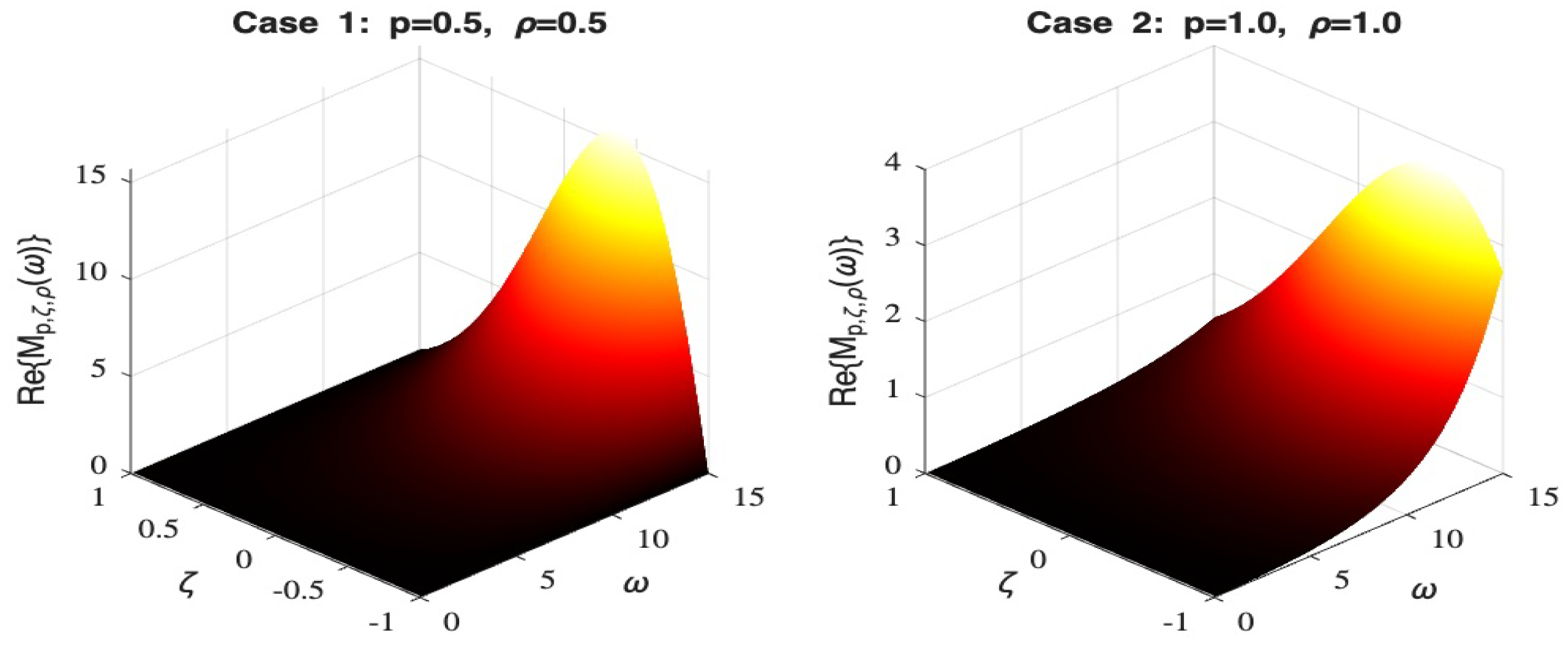
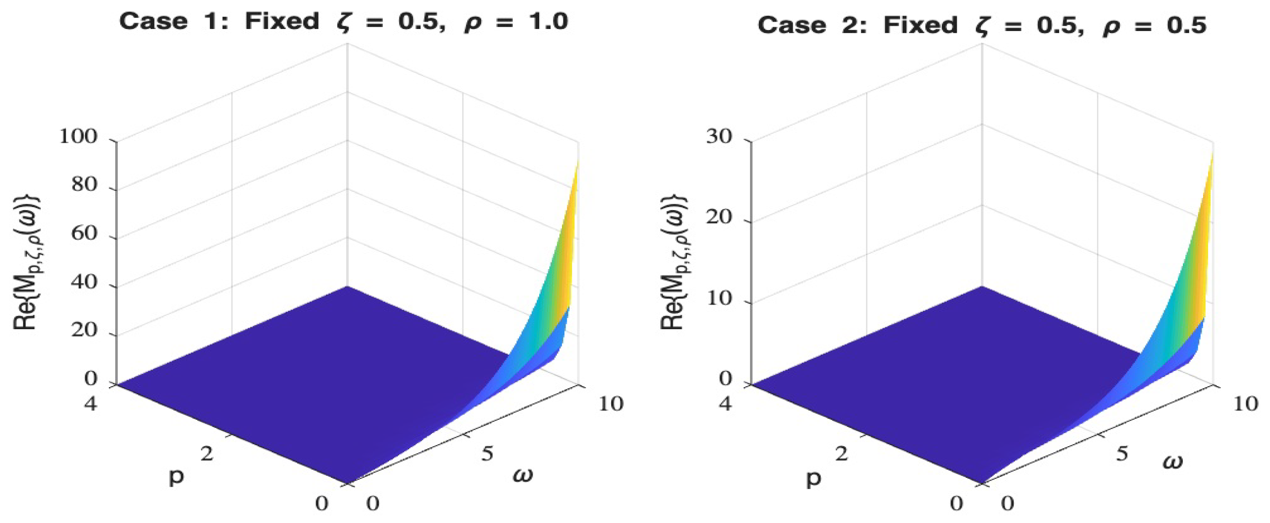
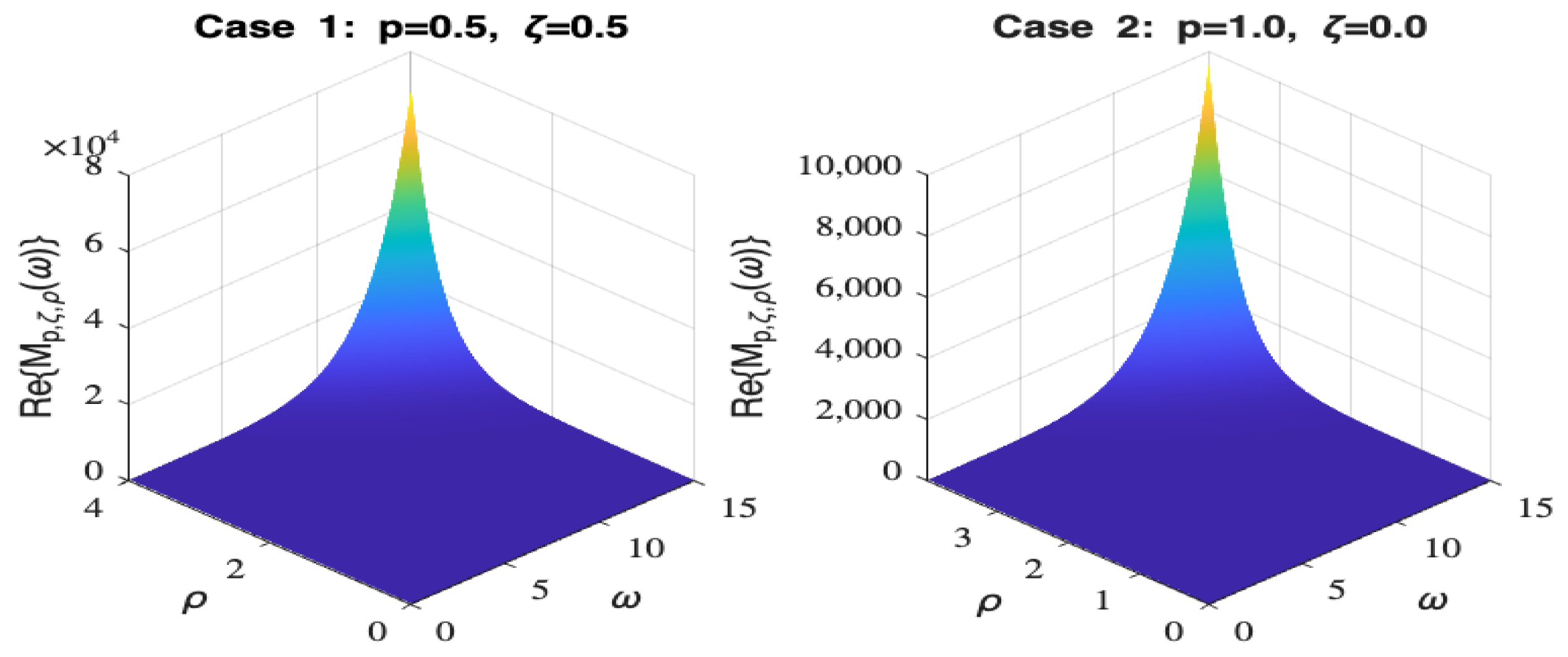
The following figures demonstrate the structural properties of the function across various parameter sets: The impact of the generalization parameter (p) on the function’s magnitude is illustrated for fixed classical parameters ($\zeta =0.5, \rho =1.0$ on the left and $\zeta =0.5, \rho =0.5$ on the right) in Figure 1. The behavior of the function with variables $\omega$ and $\rho$ for fixed pairs of p and $\zeta$ ($p=0.5, \zeta =0.5$ on the left and $p=1.0, \zeta =0$ on the right) is depicted in Figure 2. Furthermore, the influence of the $\zeta$ parameter for fixed pairs of p and $\rho$ ($p=0.5$ and $\rho =0.5$ on the left and $p=1.0$ and $\rho =1.0$ on the right) is explored in Figure 3.

These results indicate that the structural properties of the p-extended special case extend analogously to the proposed generalized function. In Figure 1, the specific case where $p=0$ successfully recovers the classical Whittaker function ${\mathrm{M}}_{\zeta ,\rho }\left(\omega \right)$, thereby validating our generalized definition. Furthermore, the plots confirm that the fundamental shape and trajectory of the function remain governed by the classical $\zeta$ and $\rho$ parameters, demonstrating the mathematical consistency of the extension.

4. Conclusions

Whittaker functions have acquired increasing significance due to their frequent use in mathematical physics applications, including studies of the Coulomb Green’s function, modeling of the hydrogen atom, and the spectral evolution resulting from the Compton scattering of radiation by hot electrons. This study derived a novel and explicit representation of the ${}_{\xi }\mathsf{\Psi }_{\eta }$-extended Whittaker function in terms of the ${}_{\xi }\mathsf{\Psi }_{\eta }$-confluent hypergeometric function. Finally, we presented a systematic study of the various fundamental properties of the proposed function, such as integral representations, a transformation formula, integral transforms, and a derivative formula. The main results, along with their special cases and consequences presented in this paper, are potentially useful in engineering sciences and mathematical physics. This work contributes to the broader understanding of special function inter-relations, enriching mathematical tools for both theoretical and applied sciences.

References

1. Erdélyi, A.; Magnus, W.; Oberhettinger, F.; Tricomi, F.G. Higher Transcendental Functions; Bateman Manuscript Project; McGraw-Hill: New York, NY, USA, 1953; Volume 1. [Google Scholar]
2. Whittaker, E.T. An expression of certain known functions as generalized hypergeometric functions. Bull. Am. Soc. 1903, 10, 125–134. [Google Scholar] [CrossRef]
3. Whittaker, E.T.; Watson, G.N. A Course of Modern Analysis, Reprint of the 4th ed.; Cambridge Mathematical Library; Cambridge University Press: Cambridge, UK, 1990. [Google Scholar]
4. Ali, M.; Ghayasuddin, M.; Khan, N.U. Certain new extension of Whittaker function and its properties. Indian J. Math. 2020, 62, 81–96. [Google Scholar]
5. Ali, M.; Ghayasuddin, M.; Khan, W.A.; Nisar, K.S. A novel kind of the multi-index Whittaker function and its certain properties. Int. J. Appl. Math. 2021, 34, 1031–1047. [Google Scholar] [CrossRef]
6. Ali, M.; Konovska, J.P.; Pogány, T.K. On multi-index Whittaker function, related integrals and inequalities. J. Math. Inequalities 2021, 16, 513–527. [Google Scholar] [CrossRef]
7. Choi, J.; Ghayasuddin, M.; Khan, N.U. Generalized extended Whittaker function and its properties. Appl. Math. Sci. 2015, 9, 6529–6541. [Google Scholar] [CrossRef]
8. Choi, J.; Nisar, K.S.; Rahman, G. An extension of Whittaker function. Commun. Korean Math. Soc. 2021, 36, 705–714. [Google Scholar] [CrossRef]
9. Khan, N.U.; Hussain, S.; Khan, M.I. Analysis of an extended Whittaker function and its properties. Honam Math. J. 2023, 45, 184–197. [Google Scholar] [CrossRef]
10. Nagar, D.K.; Morán-Vásquez, R.A.; Gupta, A.K. Properties of the extended Whittaker function. Prog. Appl. Math. 2013, 6, 70–80. [Google Scholar]
11. Chaudhry, M.A.; Qadir, A.; Rafique, M.; Zubair, S.M. Extension of Euler’s beta function. J. Comput. Appl. Math. 1997, 78, 19–32. [Google Scholar] [CrossRef]
12. Chaudhry, M.A.; Qadir, A.; Srivastava, H.M.; Paris, R.B. Extended hypergeometric and confluent hypergeometric functions. Appl. Math. Comput. 2004, 159, 589–602. [Google Scholar] [CrossRef]
13. Ghayasuddin, M.; Khan, N.U.; Ali, M. A study of extended beta, Gauss and confluent hypergeometric function. Int. J. Appl. Math. 2020, 33, 1–13. [Google Scholar] [CrossRef]
14. Ata, E.; Kiymaz, I.O. A study on certain properties of generalized special functions defined by Fox-Wright function. Appl. Math. Nonlinear Sci. 2020, 5, 147–162. [Google Scholar] [CrossRef]
15. Rainville, E.D. Special Functions; The Macmillan Company: New York, NY, USA, 1960; (Reprinted by Chelsea Publishing Company, Bronx, New York, 1971). [Google Scholar]
16. Srivastava, H.M.; Manocha, H.L. A Treatise on Generating Functions; Halsted Press (Ellis Horwood Limited, Chichester); John Wiley and Sons: New York, NY, USA, 1984. [Google Scholar]
17. Fox, C. The asymptotic expansion of generalized hypergeometric functions. Proc. Lond. Math. Soc. 1928, s2–s27, 389–400. [Google Scholar] [CrossRef]
18. Fox, C. The G and H functions as symmetrical Fourier kernels. Trans. Am. Math. Soc. 1961, 98, 395–429. [Google Scholar] [CrossRef] [PubMed]
19. Wright, E.M. The asymptotic expansion of the generalized hypergeometric function. J. Lond. Math. Soc. 1935, s1–s10, 286–293. [Google Scholar] [CrossRef]
20. Wright, E.M. The asymptotic expansion of integral functions defined by Taylor Series. Philos. Trans. R. Soc. London. Ser. A 1940, 238, 423–451. [Google Scholar] [CrossRef]
21. Wright, E.M. The asymptotic expansion of the generalized hypergeometric function II. Proc. Lond. Math. Soc. 1940, 46, 389–408. [Google Scholar] [CrossRef]
22. Kilbas, A.A.; Srivastava, H.M.; Trujillo, J.J. Theory and Applications of Fractional Differential; North-Holland Mathematics Studies 204; Elsevier: Amsterdam, The Netherlands, 2006. [Google Scholar]
23. Wiman, A. Uber den fundamental Satz in der Theorie der Funktionen E(Z). Acta Math. 1905, 29, 191–201. [Google Scholar] [CrossRef]
24. Erdélyi, A.; Magnus, W.; Oberhettinger, F.; Tricomi, F.G. Tables of Integral Transforms; McGraw-Hill: New York, NY, USA, 1954; Volume 2. [Google Scholar]
25. Erdélyi, A.; Magnus, W.; Oberhettinger, F.; Tricomi, F.G. Tables of Integral Transforms; McGraw-Hill: New York, NY, USA, 1954; Volume 1. [Google Scholar]
Figure 1. 3D plots of M p , ζ , ρ ( ω ) for fixed ζ and ρ .
Mathematics 14 00273 g001
Figure 2. 3D plots of M p , ζ , ρ ( ω ) for fixed p and ζ .
Mathematics 14 00273 g002
Figure 3. 3D plots of M p , ζ , ρ ( ω ) for fixed p and ρ .
Mathematics 14 00273 g003
Disclaimer/Publisher’s Note: The statements, opinions and data contained in all publications are solely those of the individual author(s) and contributor(s) and not of MDPI and/or the editor(s). MDPI and/or the editor(s) disclaim responsibility for any injury to people or property resulting from any ideas, methods, instructions or products referred to in the content.