Coefficient Bounds and Parameter Geometry for Gamma-Deformed Mathieu–Ma–Minda Bi-Univalent Functions

Abstract

The factorial Mathieu multiplier used in the nearest bi-univalent model is substituted with a gamma-shifted family using deformation parameter $\tau \ge 0$. In this case, one differential operator describes all class operators introduced previously, whereas the function and inverse subordination can be controlled by two different generalized Ma–Minda functions. Explicit bounds for $|a_2|$, $|a_3|$ and the Fekete–Szegő functional follow from identities involving exact second-order coefficients. These are sharpened by using the full Schwarz–Pick estimate $\left|{\omega }_2\right| \le |1-|{\omega }_1{|}^2$. The estimates continue to hold even when $\mathcal{Q}=0$. The positive-real-part, strongly starlike, Janowski, mixed Mathieu, and phase-dependent Noshiro families are included with explicit admissibility criteria, except for the Noshiro family, which has its phase limited to $-\pi <\varphi <\pi$, since ${\Delta }_2$ vanishes at the excluded endpoint. The numerical analysis compares the gamma deformation with the factorial case, partitions parameter space according to the active coefficient estimate, locates $\mathcal{Q}=0$, and shows how unequal targets displace the center of the Fekete–Szegő bound. The auxiliary Schwarz inequalities are sharp, but simultaneous equality within the full bi-univalent class is not established.

1. Introduction

Let $\mathcal{A}$ denote the family of functions analytic in the unit disk $\mathbb{D}=\{z\in \mathbb{C}:|z|<1\}$ and normalized by

$$f\left(z\right)=z+{\displaystyle \sum _{n=2}^{\infty }}{a}_n{z}^n.$$

(1)

The univalent members of $\mathcal{A}$ form the class $\mathcal{S}$. A function $f\in \mathcal{A}$ is bi-univalent when both f and its local inverse admit univalent analytic continuations to $\mathbb{D}$; the corresponding class is denoted by $\mathrm{\Sigma }$. Its inverse has the expansion

$$g\left(w\right)=f^{-1}\left(w\right)=w-a_2{w}^2+(2a_2^2-a_3)w^3-(5a_2^3-5a_2{a}_3+a_4)w^4+\cdots .$$

(2)

Initial-coefficient problems for $\mathrm{\Sigma }$ remain substantially more delicate than for $\mathcal{S}$. Lewin initiated the systematic study of $|a_2|$ [1], while Brannan and Taha developed influential bi-univalent subclasses [2]. Standard background on univalence, subordination, and the Ma–Minda framework is available in [3,4,5]. More recent operator- and special-function-generated subclasses include [6,7,8], and related determinant or polynomial constructions appear in [9,10,11]. The Fekete–Szegő functional $|a_3-\eta a_2^2|$ is retained as a principal second-order quantity [12].

Mathieu-type kernels provide a natural special-function input through Hadamard products. Mathieu’s classical series

$$S\left(r\right)={\displaystyle \sum _{n=1}^{\infty }}{\displaystyle \frac{2n}{{(n^2+r^2)}^2}},r>0,$$

(3)

originated in elasticity theory [13]; subsequent analytic inequalities and extensions are developed in [14,15,16,17,18,19,20]. Geometric applications of Mathieu-type power series include starlikeness, convexity, and Janowski-type families [21,22,23,24,25].

The direct antecedent for the present construction is the factorial generalized Mathieu bi-univalent framework of Yousef et al. [26]. Its multiplier is recovered here at $\tau =1$. The present formulation instead allows a continuous gamma shift $\tau \ge 0$, combines the earlier class-specific expressions within one nonlinear operator, and permits different generalized Ma–Minda targets on the function and inverse sides. The coefficient analysis is also arranged so that the algebraically degenerate set $\mathcal{Q}=0$ is retained rather than excluded.

Table 1. Comparison with representative closely related bi-univalent frameworks.

Study	Defining Ingredient	Relation to the Present Framework
Long et al. [6]	Generalized Mittag–Leffler function with quasi-subordination	Operator/special-function coefficient framework; the kernel is different from the Mathieu multiplier used here.
Hussen and Illafe [7]	Lucas-balancing polynomials	Polynomial-generated bi-univalent coefficient bounds; no Mathieu-series deformation is involved.
Aldawish et al. [8]	Mittag–Leffler operator with bounded boundary rotation	Another operator-defined initial-coefficient setting, but with a different special-function mechanism and class geometry.
Yousef et al. [26]	Factorial generalized Mathieu-type power-series multiplier	Direct antecedent. It is recovered at $\tau =1$; the present framework adds the gamma shift, a unified operator, unequal two-sided targets, and a nonsingular treatment of $\mathcal{Q}=0$.
Present work	Gamma-shifted Mathieu multiplier with two-sided generalized Ma–Minda subordination	Exact second-order identities, Schwarz–Pick-refined bounds, explicit degenerate-set handling, and parameter-space diagnostics within one framework.

places these features beside representative nearby operator- and special-function-based bi-univalent studies.

In this article, parameter geometry means the partition of the admissible parameter space according to the active coefficient estimate, together with the algebraic set $\mathcal{Q}=0$ and the interfaces at which candidate bounds agree. It does not denote a new geometry on the underlying function space.

The six principal contributions are as follows:

(N1)

A gamma-shifted Mathieu multiplier whose factorial model is recovered exactly at $\tau =1$, together with coefficient-level ordering and analytic well-definedness;

(N2)

A single nonlinear two-sided class operator allowing unequal generalized Ma–Minda targets for the function and its inverse;

(N3)

Exact second-order coefficient identities and Schwarz–Pick-refined estimates for $|a_2|$, $|a_3|$, and $|a_3-\eta a_2^2|$;

(N4)

A nonsingular treatment of the degenerate locus $\mathcal{Q}=0$, so the main estimates remain valid there without division by $\mathcal{Q}$;

(N5)

Unified reductions to standard positive-real-part, strongly starlike, Janowski, mixed Mathieu, and phase-dependent Noshiro-type settings, together with target-inclusion and direct transform criteria;

(N6)

Parameter-space diagnostics identifying active-bound regions, the locus $\mathcal{Q}=0$, gamma-shift sensitivity, and the displacement caused by unequal targets in the Fekete–Szegő estimate.

The determinant-type inequalities are recorded only as consequences of the initial coefficient bounds. The auxiliary Schwarz–Pick inequalities are sharp, but simultaneous sharpness for the linked full bi-univalent class is not established.

The paper is organized as follows. Section 2 introduces the multiplier and target conventions. Section 3 defines the generalized class. Section 4 derives the coefficient identities. Section 5 proves the main estimates, and Section 6 records refinements and consequences. Section 7 gives reductions and admissibility conditions. Section 8 contains direct geometric criteria, and Section 9 relates the explicit estimates to the active parameter branches and target asymmetry.

2. Preliminaries and Notation

We retain the notation $\mathcal{A}$, $\mathcal{S}$, and $\mathrm{\Sigma }$ introduced in Section 1. If

$$f\left(z\right)=z+{\displaystyle \sum _{n=2}^{\infty }}{a}_n{z}^n,h\left(z\right)=z+{\displaystyle \sum _{n=2}^{\infty }}{b}_n{z}^n,$$

then their Hadamard product is

$$(f\ast h)\left(z\right)=z+{\displaystyle \sum _{n=2}^{\infty }}{a}_n{b}_n{z}^n.$$

For functions F and G analytic in $\mathbb{D}$, we say that F is subordinate to G, written $F\prec G$, if there exists a Schwarz function $\omega$ analytic in $\mathbb{D}$ such that

$$F\left(z\right)=G\left(\omega \right(z\left)\right),\omega \left(0\right)=0,\left|\omega \right(z\left)\right|<1(z\in \mathbb{D}).$$

When G is univalent, subordination is equivalent to $F\left(0\right)=G\left(0\right)$ and $F\left(\mathbb{D}\right)\subset G\left(\mathbb{D}\right)$.

We shall use the following standard consequence of the Schwarz–Pick lemma [4]; it is recalled to fix the exact coefficient estimate used below.

Lemma 1 

(Schwarz–Pick coefficient estimate). Let $\omega \left(z\right)={\omega }_{1}z+{\omega }_2{z}^2+{\omega }_3{z}^3+\cdots$ be a Schwarz function in $\mathbb{D}$. Then

$$|{\omega }_1|\le 1,|{\omega }_2|\le 1-|{\omega }_1{|}^2\le 1.$$

In particular, $\left|{\omega }_2\right|\le 1$.

Proof. 

Schwarz’s lemma gives $\left|{\omega }_1\right|\le 1$. The function $h\left(z\right)=\omega \left(z\right)/z$, completed at $z=0$ by $h\left(0\right)={\omega }_1$, is an analytic self-map of $\mathbb{D}$ with $h^{\prime }\left(0\right)={\omega }_2$. The Schwarz–Pick inequality at the origin gives $\left|{\omega }_2\right|\le 1-|{\omega }_1{|}^2$. □

A standard Ma–Minda target is a function

$$\mathrm{\Phi }\left(z\right)=1+{\mathrm{\Phi }}_{1}z+{\mathrm{\Phi }}_2{z}^2+{\mathrm{\Phi }}_3{z}^3+\cdots$$

(4)

that is analytic and univalent in $\mathbb{D}$, satisfies $\mathrm{Re} \mathrm{\Phi }\left(z\right)>0$, $\mathrm{\Phi }\left(0\right)=1$, ${\mathrm{\Phi }}^{\prime }\left(0\right)={\mathrm{\Phi }}_1>0$, is symmetric with respect to the real axis, and maps $\mathbb{D}$ onto a domain starlike with respect to 1 [5]. The term generalized Ma–Minda target is introduced here for a target that retains analyticity, univalence, positive real part, normalization, a nonzero first coefficient, and starlikeness with respect to 1, but may omit real-axis symmetry and may have complex Taylor coefficients. This extension is needed because unequal and phase-dependent function/inverse targets need not belong to the standard real-symmetric setting.

On the function and inverse sides we allow two possibly different generalized targets,

$$\mathrm{\Phi }\left(z\right)=1+{\mathrm{\Phi }}_{1}z+{\mathrm{\Phi }}_2{z}^2+\cdots ,\mathrm{\Psi }\left(z\right)=1+{\mathrm{\Psi }}_{1}z+{\mathrm{\Psi }}_2{z}^2+\cdots ,$$

(5)

with ${\mathrm{\Phi }}_1{\mathrm{\Psi }}_1\ne 0$. The standard Ma–Minda setting is recovered when each target also satisfies the symmetry and positivity conditions above.

The Gamma- Multiplier

Let $\kappa >0$, $\ell >0$, and $\tau \ge 0$. Define

$$m_n=m_n(\kappa ,\ell ,\tau )≔{\displaystyle \frac{\mathrm{\Gamma }(n+\tau )}{\mathrm{\Gamma }(1+\tau )}}{\left({\displaystyle \frac{{\ell }^2+\mathrm{\Gamma }{(1+\tau )}^2}{{\ell }^2+\mathrm{\Gamma }{(n+\tau )}^2}}\right)}^{\kappa +1},n\ge 1.$$

(6)

Observe that $m_1=1$ and $m_n>0$. The corresponding gamma–Mathieu convolution operator is

$${\mathfrak{M}}_{\kappa ,\ell ,\tau }f\left(z\right)=z+{\displaystyle \sum _{n=2}^{\infty }}{m}_n{a}_n{z}^n.$$

(7)

For $\tau =1$, $\mathrm{\Gamma }(n+1)=n!$, and hence

$$m_n(\kappa ,\ell ,1)=n!{\left({\displaystyle \frac{{\ell }^2+1}{{\ell }^2+{(n!)}^2}}\right)}^{\kappa +1},$$

(8)

which is the normalized factorial generalized Mathieu-type multiplier used in the recently studied Mathieu bi-univalent classes [26].

The first two nontrivial coefficients are

$$m_2={\displaystyle \frac{\mathrm{\Gamma }(2+\tau )}{\mathrm{\Gamma }(1+\tau )}}{\left({\displaystyle \frac{{\ell }^2+\mathrm{\Gamma }{(1+\tau )}^2}{{\ell }^2+\mathrm{\Gamma }{(2+\tau )}^2}}\right)}^{\kappa +1},$$

(9)

$$m_3={\displaystyle \frac{\mathrm{\Gamma }(3+\tau )}{\mathrm{\Gamma }(1+\tau )}}{\left({\displaystyle \frac{{\ell }^2+\mathrm{\Gamma }{(1+\tau )}^2}{{\ell }^2+\mathrm{\Gamma }{(3+\tau )}^2}}\right)}^{\kappa +1}.$$

(10)

Remark 1 

(Contribution of the gamma shift). The value $\tau =1$ gives the factorial multiplier exactly, whereas $\tau \ne 1$ changes both the gamma prefactor and the denominator ratio in every $m_n$. Thus τ is not a constant rescaling of the earlier operator: it changes the relative suppression of the Taylor modes and, through $m_2$ and $m_3$, moves the coefficient-bound interfaces and the set $\mathcal{Q}=0$.

The next lemma verifies that the multiplier defines an analytic transform for every $f\in \mathcal{A}$ and justifies the termwise coefficient comparisons used later. Its tail statement quantifies the smoothing effect on compact subdisks; it is not a compactness assertion in an unspecified function-space topology.

Lemma 2 

(Well-definedness and smoothing). For every $f\in \mathcal{A}$, the series (7) defines an analytic function in $\mathbb{D}$. Moreover, for each $0<R<1$, the operator ${\mathfrak{M}}_{\kappa ,\ell ,\tau }$ maps locally bounded families in $\mathcal{A}$ into families whose coefficient tails are uniformly suppressed on $\left|z\right|\le R$.

Proof. 

Fix $0<R<R_1<1$. Cauchy’s estimate gives $\left|a_n\right|\le C_{R_1}{R}_1^{-n}$. From (6),

$$0<m_n\le C_{\kappa ,\ell ,\tau }\mathrm{\Gamma }{(n+\tau )}^{-(2\kappa +1)}.$$

Consequently,

$$|m_n{a}_n|R^n\le C_{R_1}{C}_{\kappa ,\ell ,\tau }\mathrm{\Gamma }{(n+\tau )}^{-(2\kappa +1)}{\left({\displaystyle \frac{R}{R_1}}\right)}^n.$$

The right-hand side is summable, so the multiplier series converges absolutely and uniformly on $\left|z\right|\le R$. If f ranges over a locally bounded family, Cauchy’s constant can be chosen uniformly on $\left|z\right|\le R_1$; the same majorant then shows that the tails beginning at $n=N$ converge uniformly to zero as $N\to \infty$. □

Proposition 1 

(Multiplier ordering). Fix $n\ge 2$ and $\tau \ge 0$, and suppose that $\mathrm{\Gamma }(n+\tau )>\mathrm{\Gamma }(1+\tau )$. Then

(i) 

For every $\ell >0$, $m_n(\kappa ,\ell ,\tau )$ is strictly decreasing in $\kappa >0$;

(ii) 

For every $\kappa >0$, $m_n(\kappa ,\ell ,\tau )$ is strictly increasing in $\ell >0$.

Proof. 

Set $a=\mathrm{\Gamma }(1+\tau )$, $b=\mathrm{\Gamma }(n+\tau )$, and

$$R_n(\ell )={\displaystyle \frac{{\ell }^2+a^2}{{\ell }^2+b^2}}.$$

The hypothesis $b>a$ gives $0<R_n(\ell )<1$. Since

$$m_n={\displaystyle \frac{b}{a}}{R}_n{(\ell )}^{\kappa +1},$$

we have

$${\displaystyle \frac{\partial m_n}{\partial \kappa }}=m_n\log R_n(\ell )<0,$$

which proves (i). Moreover,

$${\displaystyle \frac{d}{d\ell }}\log R_n(\ell )={\displaystyle \frac{2\ell }{{\ell }^2+a^2}}-{\displaystyle \frac{2\ell }{{\ell }^2+b^2}}={\displaystyle \frac{2\ell (b^2-a^2)}{({\ell }^2+a^2)({\ell }^2+b^2)}}>0.$$

Therefore $\partial m_n/\partial \ell >0$, proving (ii). □

Remark 2. 

Proposition 1 orders the multiplier coefficients themselves. It does not imply a global monotonicity theorem for the final bounds, because those bounds contain $m_2$, $m_3$, and the denominator $\mathcal{Q}$ in competing combinations. Numerical trends are therefore stated only for the parameter ranges displayed.

3. The Generalized Mathieu–Ma–Minda Class

Let F be analytic in $\mathbb{D}$, normalized by $F\left(0\right)=0$, $F^{\prime }\left(0\right)=1$, and write

$$F\left(z\right)=z+A_2{z}^2+A_3{z}^3+\cdots .$$

(11)

For real parameters $\delta ,\mu ,\nu$ and a complex parameter $\beta$, define

$${\mathcal{J}}_{\delta ,\mu ,\nu ,\beta }F\left(z\right)=(1-\delta ){\left({\displaystyle \frac{F\left(z\right)}{z}}\right)}^{\mu }+\delta {\left(F^{\prime }\left(z\right)\right)}^{\nu }+\beta z{F}^{″}\left(z\right).$$

(12)

Remark 3 

(Analytic branch convention). When μ and ν are non-integer real numbers, the powers in (12) require analytic branches. Thus, in the definition below, the functions $F\left(z\right)/z$ and $F^{\prime }\left(z\right)$ are required to be nonzero in $\mathbb{D}$, and the powers are understood with the analytic branch determined by the value 1 at the origin. If μ and ν are nonnegative integers, no branch restriction is needed. This convention corrects a common hidden gap in definitions involving fractional powers of normalized analytic expressions.

A direct binomial expansion, detailed in Appendix A, yields

$${\mathcal{J}}_{\delta ,\mu ,\nu ,\beta }F\left(z\right)=1+{\Delta }_1{A}_{2}z+\left({\Delta }_2{A}_3+{\Delta }_3{A}_2^2\right)z^2+O\left(z^3\right),$$

(13)

where

$$\begin{array}{cc}\hfill {\Delta }_1& =(1-\delta )\mu +2\delta \nu +2\beta ,\hfill \end{array}$$

(14)

$$\begin{array}{cc}\hfill {\Delta }_2& =(1-\delta )\mu +3\delta \nu +6\beta ,\hfill \end{array}$$

(15)

$$\begin{array}{cc}\hfill {\Delta }_3& ={\displaystyle \frac{1-\delta }{2}}\mu (\mu -1)+2\delta \nu (\nu -1).\hfill \end{array}$$

(16)

Definition 1. 

Let Φ and Ψ be generalized Ma–Minda targets of the form (5). A function $f\in \mathrm{\Sigma }$, given by (1), belongs to

$${\mathcal{B}}_{\mathrm{\Sigma }}^{\kappa ,\ell ,\tau }(\delta ,\mu ,\nu ,\beta ;\mathrm{\Phi },\mathrm{\Psi })$$

if the following two subordinations hold:

$${\mathcal{J}}_{\delta ,\mu ,\nu ,\beta }\left({\mathfrak{M}}_{\kappa ,\ell ,\tau }f\right)\left(z\right)\prec \mathrm{\Phi }\left(z\right),z\in \mathbb{D},$$

(17)

$${\mathcal{J}}_{\delta ,\mu ,\nu ,\beta }\left({\mathfrak{M}}_{\kappa ,\ell ,\tau }g\right)\left(w\right)\prec \mathrm{\Psi }\left(w\right),w\in \mathbb{D},$$

(18)

where $g=f^{-1}$ is given by (2). When fractional powers occur, the branch convention of Remark 3 is imposed for ${\mathfrak{M}}_{\kappa ,\ell ,\tau }f$ and ${\mathfrak{M}}_{\kappa ,\ell ,\tau }g$.

Remark 4 

(Non-emptiness). The class in Definition 1 is nonempty for every admissible parameter choice. Indeed, the identity $f\left(z\right)=z$, whose inverse is also the identity, satisfies ${\mathfrak{M}}_{\kappa ,\ell ,\tau }f\left(z\right)=z$ and ${\mathcal{J}}_{\delta ,\mu ,\nu ,\beta }\left({\mathfrak{M}}_{\kappa ,\ell ,\tau }f\right)=1$ on both sides. The required subordinations follow by taking the Schwarz functions $u\equiv v\equiv 0$.

Remark 5 

(Relation with earlier Mathieu classes). Definition 1 contains the classes in [26] as special cases. Taking $\tau =1$ recovers the factorial Mathieu multiplier. Taking $\nu =1-\mu$ gives the mixed expression involving ${(F/z)}^{\mu }$, ${\left(F^{\prime }\right)}^{1-\mu }$ and $z{F}^{″}$. Taking $\delta =1$, $\mu =0$, $\nu =1$ and $\beta =e^{i\varphi }+1/2$ gives the phase-dependent Noshiro-type expression

$$F^{\prime }\left(z\right)+\left(e^{i\varphi }+{\displaystyle \frac{1}{2}}\right)z{F}^{″}\left(z\right).$$

The phase-dependent coefficient constants and admissible interval are rederived in Section 7.

The following standard targets illustrate how the generalized definition specializes to the principal geometric subclasses used in Section 7.

Example 1 

(Janowski target). For $-1\le B<A\le 1$,

$${\mathrm{\Phi }}_{A,B}\left(z\right)={\displaystyle \frac{1+Az}{1+Bz}}=1+(A-B)z+(B^2-AB)z^2+\cdots .$$

(19)

This is the standard Janowski target and covers many starlike and half-plane cases.

Example 2 

(Positive-real-part target of order $\rho$). For $0\le \rho <1$,

$${\mathrm{\Phi }}_{\rho }\left(z\right)={\displaystyle \frac{1+(1-2\rho )z}{1-z}}=1+2(1-\rho )z+2(1-\rho )z^2+\cdots .$$

(20)

The condition $p\prec {\mathrm{\Phi }}_{\rho }$ implies $\mathrm{Re} p\left(z\right)>\rho$.

Example 3 

(Strongly starlike target). For $0<\alpha \le 1$,

$${\mathrm{\Phi }}_{\alpha }\left(z\right)={\left({\displaystyle \frac{1+z}{1-z}}\right)}^{\alpha }=1+2\alpha z+2{\alpha }^2{z}^2+\cdots .$$

(21)

This target maps the unit disk into the sector $|\arg w|<\alpha \pi /2$.

4. Coefficient Identities

Before deriving estimates, we write down the full second-order coefficient system. This makes the proof transparent and prevents the common ambiguity between the coefficients of f, the coefficients of the target functions and the coefficients of the Schwarz functions.

Let

$$H\left(z\right)={\mathfrak{M}}_{\kappa ,\ell ,\tau }f\left(z\right),G\left(w\right)={\mathfrak{M}}_{\kappa ,\ell ,\tau }g\left(w\right).$$

Using (1) and (2), we have

$$H\left(z\right)=z+m_2{a}_2{z}^2+m_3{a}_3{z}^3+\cdots ,$$

(22)

$$G\left(w\right)=w-m_2{a}_2{w}^2+m_3(2a_2^2-a_3)w^3+\cdots .$$

(23)

By Definition 1, there exist Schwarz functions

$$u\left(z\right)=u_{1}z+u_2{z}^2+\cdots ,v\left(w\right)=v_{1}w+v_2{w}^2+\cdots$$

(24)

such that

$${\mathcal{J}}_{\delta ,\mu ,\nu ,\beta }H\left(z\right)=\mathrm{\Phi }\left(u\left(z\right)\right),{\mathcal{J}}_{\delta ,\mu ,\nu ,\beta }G\left(w\right)=\mathrm{\Psi }\left(v\left(w\right)\right).$$

(25)

The target expansions are

$$\mathrm{\Phi }\left(u\left(z\right)\right)=1+{\mathrm{\Phi }}_1{u}_{1}z+({\mathrm{\Phi }}_1{u}_2+{\mathrm{\Phi }}_2{u}_1^2)z^2+O\left(z^3\right),$$

(26)

$$\mathrm{\Psi }\left(v\left(w\right)\right)=1+{\mathrm{\Psi }}_1{v}_{1}w+({\mathrm{\Psi }}_1{v}_2+{\mathrm{\Psi }}_2{v}_1^2)w^2+O\left(w^3\right).$$

(27)

Combining (13)–(27) gives

$${\Delta }_1{m}_2{a}_2={\mathrm{\Phi }}_1{u}_1,$$

(28)

$${\Delta }_2{m}_3{a}_3+{\Delta }_3{m}_2^2{a}_2^2={\mathrm{\Phi }}_1{u}_2+{\mathrm{\Phi }}_2{u}_1^2,$$

(29)

$$-{\Delta }_1{m}_2{a}_2={\mathrm{\Psi }}_1{v}_1,$$

(30)

$${\Delta }_2{m}_3(2a_2^2-a_3)+{\Delta }_3{m}_2^2{a}_2^2={\mathrm{\Psi }}_1{v}_2+{\mathrm{\Psi }}_2{v}_1^2.$$

(31)

Consequently,

$$u_1^2={\displaystyle \frac{{\Delta }_1^2{m}_2^2}{{\mathrm{\Phi }}_1^2}}{a}_2^2,v_1^2={\displaystyle \frac{{\Delta }_1^2{m}_2^2}{{\mathrm{\Psi }}_1^2}}{a}_2^2.$$

(32)

5. Main Coefficient Estimates

• Standing assumptions.

Unless otherwise stated, throughout this section the parameters satisfy $\kappa >0$, $\ell >0$, $\tau \ge 0$, and $\delta ,\mu ,\nu \in \mathbb{R}$, while $\beta \in \mathbb{C}$. The target functions $\mathrm{\Phi }$ and $\mathrm{\Psi }$ are generalized Ma–Minda targets with ${\mathrm{\Phi }}_1{\mathrm{\Psi }}_1\ne 0$. If $\mu$ or $\nu$ is not an integer, the analytic branch convention stated in Remark 3 is imposed. The coefficient estimates below also require

$${\Delta }_1{\Delta }_2{m}_2{m}_3\ne 0.$$

(33)

Here $m_2,m_3>0$, but ${\Delta }_1$, ${\Delta }_2$, and $\mathcal{Q}$ may be complex when $\beta$ is complex; all estimates are therefore written in modulus. In applications where a convex combination of the two first-order expressions is desired, one may restrict to $0\le \delta \le 1$, but the algebraic coefficient identities remain valid for every real $\delta$.

Define

$$\mathcal{Q}≔2({\Delta }_2{m}_3+{\Delta }_3{m}_2^2)-{\Delta }_1^2{m}_2^2\left({\displaystyle \frac{{\mathrm{\Phi }}_2}{{\mathrm{\Phi }}_1^2}}+{\displaystyle \frac{{\mathrm{\Psi }}_2}{{\mathrm{\Psi }}_1^2}}\right).$$

(34)

Theorem 1 

(Schwarz–Pick-refined estimate for $|a_2|$). Let $\kappa >0$, $\ell >0$, $\tau \ge 0$, $\delta ,\mu ,\nu \in \mathbb{R}$, and $\beta \in \mathbb{C}$. Let Φ and Ψ be generalized Ma–Minda targets with ${\mathrm{\Phi }}_1{\mathrm{\Psi }}_1{\Delta }_1\ne 0$, impose the branch convention of Remark 3 when required, and let $f\in {\mathcal{B}}_{\mathrm{\Sigma }}^{\kappa ,\ell ,\tau }(\delta ,\mu ,\nu ,\beta ;\mathrm{\Phi },\mathrm{\Psi })$. Then

$$\left|a_2\right|\le {\rho }_2,$$

(35)

where

$${\rho }_2≔\min \left\{{\displaystyle \frac{|{\mathrm{\Phi }}_1|}{|{\Delta }_1|m_2}},{\displaystyle \frac{|{\mathrm{\Psi }}_1|}{|{\Delta }_1|m_2}},\sqrt{{\displaystyle \frac{|{\mathrm{\Phi }}_1|+|{\mathrm{\Psi }}_1|}{\left|\mathcal{Q}\right|+|{\Delta }_1{|}^2{m}_2^2({\left|{\mathrm{\Phi }}_1\right|}^{-1}+|{\mathrm{\Psi }}_1{|}^{-1})}}}\right\}.$$

(36)

In particular, the estimate is valid when $\mathcal{Q}=0$.

Proof. 

By the first coefficient comparisons (28) and (30), we have

$$a_2={\displaystyle \frac{{\mathrm{\Phi }}_1{u}_1}{{\Delta }_1{m}_2}}=-{\displaystyle \frac{{\mathrm{\Psi }}_1{v}_1}{{\Delta }_1{m}_2}}.$$

Since u and v are Schwarz functions, Lemma 1 gives $\left|u_1\right|\le 1$ and $\left|v_1\right|\le 1$. Hence

$$|a_2|\le {\displaystyle \frac{\left|{\mathrm{\Phi }}_1\right|}{\left|{\Delta }_1\right|m_2}},\left|a_2\right|\le {\displaystyle \frac{\left|{\mathrm{\Psi }}_1\right|}{\left|{\Delta }_1\right|m_2}}.$$

These are the two elementary first-order estimates.

A third estimate is obtained from the second-order equations. Adding (29) and (31) eliminates $a_3$ and gives

$$2({\Delta }_2{m}_3+{\Delta }_3{m}_2^2)a_2^2={\mathrm{\Phi }}_1{u}_2+{\mathrm{\Psi }}_1{v}_2+{\mathrm{\Phi }}_2{u}_1^2+{\mathrm{\Psi }}_2{v}_1^2.$$

Using (32), namely

$$u_1^2={\displaystyle \frac{{\Delta }_1^2{m}_2^2}{{\mathrm{\Phi }}_1^2}}{a}_2^2,v_1^2={\displaystyle \frac{{\Delta }_1^2{m}_2^2}{{\mathrm{\Psi }}_1^2}}{a}_2^2,$$

we move the terms containing $a_2^2$ to the left-hand side and obtain

$$\left\{2({\Delta }_2{m}_3+{\Delta }_3{m}_2^2)-{\Delta }_1^2{m}_2^2\left({\displaystyle \frac{{\mathrm{\Phi }}_2}{{\mathrm{\Phi }}_1^2}}+{\displaystyle \frac{{\mathrm{\Psi }}_2}{{\mathrm{\Psi }}_1^2}}\right)\right\}{a}_2^2={\mathrm{\Phi }}_1{u}_2+{\mathrm{\Psi }}_1{v}_2.$$

The expression in braces is exactly $\mathcal{Q}$. Taking moduli in $\mathcal{Q}{a}_2^2={\mathrm{\Phi }}_1{u}_2+{\mathrm{\Psi }}_1{v}_2$ and using the full estimate in Lemma 1, together with (28) and (30), gives

$$\left|\mathcal{Q}\right|{|a_2|}^2\le \left|{\mathrm{\Phi }}_1\right|(1-{|u_1|}^2)+|{\mathrm{\Psi }}_1|(1-{|v_1|}^2).$$

Hence

$$\left[|\mathcal{Q}|+|{\Delta }_1{|}^2{m}_2^2\left({\displaystyle \frac{1}{|{\mathrm{\Phi }}_1|}}+{\displaystyle \frac{1}{|{\mathrm{\Psi }}_1|}}\right)\right]|a_2{|}^2\le |{\mathrm{\Phi }}_1|+|{\mathrm{\Psi }}_1|.$$

Combining the square root of this inequality with the two first-order estimates proves (36). No division by $\mathcal{Q}$ has been used. □

Theorem 2 

(Estimate for $|a_3|$). Let all parameters, targets, and branch choices satisfy the hypotheses of Theorem 1, assume additionally that ${\Delta }_2\ne 0$, and let f belong to the class stated there. Then

$$\left|a_3\right|\le C+\max \{0,|{\Lambda }_0|-D\}{\rho }_2^2,$$

(37)

where

$${\Lambda }_{\eta }≔1-\eta +{\displaystyle \frac{{\Delta }_1^2{m}_2^2}{2{\Delta }_2{m}_3}}\left({\displaystyle \frac{{\mathrm{\Phi }}_2}{{\mathrm{\Phi }}_1^2}}-{\displaystyle \frac{{\mathrm{\Psi }}_2}{{\mathrm{\Psi }}_1^2}}\right),$$

(38)

$$C≔{\displaystyle \frac{|{\mathrm{\Phi }}_1|+|{\mathrm{\Psi }}_1|}{2|{\Delta }_2|m_3}},D≔{\displaystyle \frac{|{\Delta }_1{|}^2{m}_2^2}{2|{\Delta }_2|m_3}}\left({\displaystyle \frac{1}{|{\mathrm{\Phi }}_1|}}+{\displaystyle \frac{1}{|{\mathrm{\Psi }}_1|}}\right).$$

(39)

Proof. 

Subtract (31) from (29). The terms containing ${\Delta }_3{m}_2^2{a}_2^2$ cancel, and the left-hand side becomes

$${\Delta }_2{m}_3{a}_3-{\Delta }_2{m}_3(2a_2^2-a_3)=2{\Delta }_2{m}_3(a_3-a_2^2).$$

Therefore

$$2{\Delta }_2{m}_3(a_3-a_2^2)={\mathrm{\Phi }}_1{u}_2-{\mathrm{\Psi }}_1{v}_2+{\mathrm{\Phi }}_2{u}_1^2-{\mathrm{\Psi }}_2{v}_1^2.$$

Substituting (32) into the last two terms gives

$$2{\Delta }_2{m}_3(a_3-a_2^2)={\mathrm{\Phi }}_1{u}_2-{\mathrm{\Psi }}_1{v}_2+{\Delta }_1^2{m}_2^2\left({\displaystyle \frac{{\mathrm{\Phi }}_2}{{\mathrm{\Phi }}_1^2}}-{\displaystyle \frac{{\mathrm{\Psi }}_2}{{\mathrm{\Psi }}_1^2}}\right)a_2^2.$$

Since ${\Delta }_2{m}_3\ne 0$, division by $2{\Delta }_2{m}_3$ gives the identity

$$a_3=\left[1+{\displaystyle \frac{{\Delta }_1^2{m}_2^2}{2{\Delta }_2{m}_3}}\left({\displaystyle \frac{{\mathrm{\Phi }}_2}{{\mathrm{\Phi }}_1^2}}-{\displaystyle \frac{{\mathrm{\Psi }}_2}{{\mathrm{\Psi }}_1^2}}\right)\right]a_2^2+{\displaystyle \frac{{\mathrm{\Phi }}_1{u}_2-{\mathrm{\Psi }}_1{v}_2}{2{\Delta }_2{m}_3}}.$$

Taking absolute values, applying Lemma 1, and using the first-order identities gives

$$\left|a_3\right|\le C+\left(\right|{\Lambda }_0|-D)|a_2{|}^2.$$

Since $0 \le {\left|a_2\right|}^2 \le {\rho }_2^2$, maximizing this affine expression over the indicated interval gives (37). □

Theorem 3 

(Fekete–Szego inequality). Let all parameters, targets, and branch choices satisfy the hypotheses of Theorem 1, assume ${\Delta }_2\ne 0$, let f belong to the class stated there, and let $\eta \in \mathbb{C}$. Then

$$|a_3-\eta a_2^2|\le C+\max \{0,|{\Lambda }_{\eta }|-D\}{\rho }_2^2,$$

(40)

where ${\Lambda }_{\eta }$, C, and D are given by (38) and (39). If $\mathrm{\Phi }=\mathrm{\Psi }$, then

$$|a_3-\eta a_2^2|\le C_{\mathrm{\Phi }}+\max \{0,|1-\eta |-C_{\mathrm{\Phi }}{R}_{\mathrm{\Phi }}\}{\rho }_2^2,$$

(41)

where $C_{\mathrm{\Phi }}=\left|{\mathrm{\Phi }}_1\right|/\left(\right|{\Delta }_2\left|m_3\right)$ and $R_{\mathrm{\Phi }}={\left|{\Delta }_1\right|}^2{m}_2^2/{\left|{\mathrm{\Phi }}_1\right|}^2$.

Proof. 

From the identity obtained in the proof of Theorem 2,

$$a_3=\left[1+{\displaystyle \frac{{\Delta }_1^2{m}_2^2}{2{\Delta }_2{m}_3}}\left({\displaystyle \frac{{\mathrm{\Phi }}_2}{{\mathrm{\Phi }}_1^2}}-{\displaystyle \frac{{\mathrm{\Psi }}_2}{{\mathrm{\Psi }}_1^2}}\right)\right]a_2^2+{\displaystyle \frac{{\mathrm{\Phi }}_1{u}_2-{\mathrm{\Psi }}_1{v}_2}{2{\Delta }_2{m}_3}}.$$

Subtracting $\eta a_2^2$ gives

$$a_3-\eta a_2^2=\left[1-\eta +{\displaystyle \frac{{\Delta }_1^2{m}_2^2}{2{\Delta }_2{m}_3}}\left({\displaystyle \frac{{\mathrm{\Phi }}_2}{{\mathrm{\Phi }}_1^2}}-{\displaystyle \frac{{\mathrm{\Psi }}_2}{{\mathrm{\Psi }}_1^2}}\right)\right]a_2^2+{\displaystyle \frac{{\mathrm{\Phi }}_1{u}_2-{\mathrm{\Psi }}_1{v}_2}{2{\Delta }_2{m}_3}}.$$

The triangle inequality and Lemma 1 give

$$|a_3-\eta a_2^2|\le |{\Lambda }_{\eta }|{|a_2|}^2+{\displaystyle \frac{|{\mathrm{\Phi }}_1\left|\right(1-\left|u_1{|}^2)+|{\mathrm{\Psi }}_1\right|(1-|v_1{|}^2)}{2|{\Delta }_2|m_3}}.$$

Therefore

$$|a_3-\eta a_2^2|\le C+\left(\right|{\Lambda }_{\eta }|-D){\left|a_2\right|}^2.$$

Maximizing over $0\le {\left|a_2\right|}^2\le {\rho }_2^2$ proves (40).

If $\mathrm{\Phi }=\mathrm{\Psi }$, then ${\Lambda }_{\eta }=1-\eta$, $C=C_{\mathrm{\Phi }}$, and $D=C_{\mathrm{\Phi }}{R}_{\mathrm{\Phi }}$, which gives (41). □

Proposition 2 

(Degenerate set $\mathcal{Q}=0$). Let f satisfy the hypotheses of Theorem 1 and suppose that $\mathcal{Q}=0$. Then

$$|a_2|\le \min \left\{{\displaystyle \frac{|{\mathrm{\Phi }}_1|}{|{\Delta }_1|m_2}},{\displaystyle \frac{|{\mathrm{\Psi }}_1|}{|{\Delta }_1|m_2}}\right\}.$$

(42)

If also ${\Delta }_2\ne 0$, the estimates (37) and (40) remain valid with the same value of ${\rho }_2$.

Proof. 

When $\mathcal{Q}=0$, the third candidate in (36) reduces to

$${\displaystyle \frac{\sqrt{|{\mathrm{\Phi }}_1{\mathrm{\Psi }}_1|}}{|{\Delta }_1|m_2}}.$$

This quantity is not smaller than the minimum of the first two candidates, so (36) reduces to (42). The proofs of Theorems 2 and 3 do not divide by $\mathcal{Q}$; their conclusions therefore remain valid. □

6. Additional Coefficient Consequences

This section derives additional estimates from the same second-order coefficient system. These statements should be read as consequences of the obtained $|a_2|$ and $|a_3|$ bounds, not as independent sharp determinant theorems.

6.1. Sharpness Status and Auxiliary Extremals

The coefficient estimate in Lemma 1 is sharp within the family of Schwarz functions. For $a\in \mathbb{D}$ and $\theta \in \mathbb{R}$, the degree-two Blaschke product

$${\omega }_{a,\theta }\left(z\right)=z{e}^{i\theta }{\displaystyle \frac{a-z}{1-\overline{a}z}}$$

satisfies $\left|{\omega }_1\right|=\left|a\right|$ and $|{\omega }_2|=1-{\left|a\right|}^2$. Thus the Schwarz–Pick step used in Theorems 1–3 cannot be improved without exploiting additional compatibility between the two subordinations.

This auxiliary equality does not by itself produce an extremal member of the class in Definition 1. The functions u and v are linked by (28)–(31) and must arise from the same bi-univalent function through two global subordinations. No simultaneous equality construction is presently known for the full parameter family. Accordingly, the estimates proved here are refined and explicit, but they are not claimed to be sharp for the full class.

6.2. Inverse Coefficient Estimates

Let

$$g\left(w\right)=f^{-1}\left(w\right)=w+b_2{w}^2+b_3{w}^3+\cdots .$$

Then $b_2=-a_2$ and $b_3=2a_2^2-a_3$. The following result is useful when the inverse mapping itself is the object of study.

Proposition 3 

(Inverse coefficients). Let f satisfy the hypotheses of Theorem 3. Then

$$\left|b_2\right|\le {\rho }_2,$$

(43)

and

$$\left|b_3\right|\le C+\max \{0,|{\Lambda }_2|-D\}{\rho }_2^2.$$

(44)

Proof. 

The inverse expansion (2) gives

$$b_2=-a_2,b_3=2a_2^2-a_3.$$

Therefore Theorem 1 immediately yields

$$\left|b_2\right|=\left|a_2\right|\le {\rho }_2.$$

Since $b_3=-(a_3-2a_2^2)$, estimate (44) is Theorem 3 with $\eta =2$. □

6.3. Logarithmic Coefficients

The logarithmic coefficients ${\gamma }_n$ of f are defined by

$$\log {\displaystyle \frac{f\left(z\right)}{z}}=2{\displaystyle \sum _{n=1}^{\infty }}{\gamma }_n{z}^n.$$

(45)

From the expansion of the logarithm,

$${\gamma }_1={\displaystyle \frac{a_2}{2}},{\gamma }_2={\displaystyle \frac{1}{2}}\left(a_3-{\displaystyle \frac{1}{2}}{a}_2^2\right).$$

(46)

Theorem 4 

(First logarithmic coefficients). Let f satisfy the hypotheses of Theorem 3. Then the logarithmic coefficients satisfy

$$|{\gamma }_1|\le {\displaystyle \frac{{\rho }_2}{2}},$$

(47)

and

$$|{\gamma }_2|\le {\displaystyle \frac{1}{2}}\left[C+\max \{0,|{\Lambda }_{1/2}|-D\}{\rho }_2^2\right].$$

(48)

Proof. 

From (45),

$$\log {\displaystyle \frac{f\left(z\right)}{z}}=\log (1+a_{2}z+a_3{z}^2+\cdots ).$$

Using $\log (1+X)=X-X^2/2+O\left(X^3\right)$, with $X=a_{2}z+a_3{z}^2+O\left(z^3\right)$, gives

$$\log {\displaystyle \frac{f\left(z\right)}{z}}=a_{2}z+\left(a_3-{\displaystyle \frac{1}{2}}{a}_2^2\right)z^2+O\left(z^3\right).$$

Comparing this with $2{\sum }_{n=1}^{\infty }{\gamma }_n{z}^n$, we obtain

$${\gamma }_1={\displaystyle \frac{a_2}{2}},{\gamma }_2={\displaystyle \frac{1}{2}}\left(a_3-{\displaystyle \frac{1}{2}}{a}_2^2\right).$$

The first estimate follows immediately from Theorem 1:

$$|{\gamma }_1|={\displaystyle \frac{|a_2|}{2}}\le {\displaystyle \frac{{\rho }_2}{2}}.$$

For ${\gamma }_2$, apply the Fekete–Szego estimate (40) with $\eta =1/2$. Since

$$|{\gamma }_2|={\displaystyle \frac{1}{2}}\left|a_3-{\displaystyle \frac{1}{2}}{a}_2^2\right|,$$

dividing the resulting inequality by 2 gives (48). □

6.4. Derived Zalcman and Determinant Inequalities

The following estimates are direct consequences of the preceding second-order coefficient bounds. They are not asserted to be sharp determinant theorems.

Corollary 1 

(Derived determinant bounds). Let f satisfy the hypotheses of Theorem 3, and define

$${\mathcal{B}}_3≔C+\max \{0,|{\Lambda }_0|-D\}{\rho }_2^2.$$

(49)

Then

$$|a_3-a_2^2|\le C+\max \{0,|{\Lambda }_1|-D\}{\rho }_2^2.$$

(50)

If $T_2\left(2\right)=a_2^2-a_3^2$ and

$$T_3\left(1\right)=\det \left(\begin{array}{ccc}1& a_2& a_3\\ a_2& 1& a_2\\ a_3& a_2& 1\end{array}\right),$$

then

$$|T_2\left(2\right)|\le {\rho }_2^2+{\mathcal{B}}_3^2,$$

(51)

$$|T_3\left(1\right)|\le 1+2{\rho }_2^2+2{\rho }_2^2{\mathcal{B}}_3+{\mathcal{B}}_3^2.$$

(52)

Proof. 

Equation (50) is Theorem 3 with $\eta =1$. Theorem 2 gives $\left|a_3\right|\le {\mathcal{B}}_3$, while Theorem 1 gives $|a_2|\le {\rho }_2$. Hence

$$|T_2(2)|\le {\left|a_2\right|}^2+{\left|a_3\right|}^2\le {\rho }_2^2+{\mathcal{B}}_3^2.$$

Finally, $T_3\left(1\right)=1-2a_2^2+2a_2^2{a}_3-a_3^2$; the triangle inequality yields (52). □

6.5. Inclusion Under Target Domination

Proposition 4 

(Target inclusion). Let $\mathrm{\Phi },\mathrm{\Psi },\tilde{\mathrm{\Phi }},\tilde{\mathrm{\Psi }}$ be generalized Ma–Minda targets. If

$$\mathrm{\Phi }\prec \tilde{\mathrm{\Phi }},\mathrm{\Psi }\prec \tilde{\mathrm{\Psi }},$$

then

$${\mathcal{B}}_{\mathrm{\Sigma }}^{\kappa ,\ell ,\tau }(\delta ,\mu ,\nu ,\beta ;\mathrm{\Phi },\mathrm{\Psi })\subset {\mathcal{B}}_{\mathrm{\Sigma }}^{\kappa ,\ell ,\tau }(\delta ,\mu ,\nu ,\beta ;\tilde{\mathrm{\Phi }},\tilde{\mathrm{\Psi }}).$$

Proof. 

Let $f\in {\mathcal{B}}_{\mathrm{\Sigma }}^{\kappa ,\ell ,\tau }(\delta ,\mu ,\nu ,\beta ;\mathrm{\Phi },\mathrm{\Psi })$, and let $g=f^{-1}$. By definition of the class,

$${\mathcal{J}}_{\delta ,\mu ,\nu ,\beta }\left({\mathfrak{M}}_{\kappa ,\ell ,\tau }f\right)\prec \mathrm{\Phi },{\mathcal{J}}_{\delta ,\mu ,\nu ,\beta }\left({\mathfrak{M}}_{\kappa ,\ell ,\tau }g\right)\prec \mathrm{\Psi }.$$

The assumptions $\mathrm{\Phi }\prec \tilde{\mathrm{\Phi }}$ and $\mathrm{\Psi }\prec \tilde{\mathrm{\Psi }}$ mean that there exist Schwarz functions ${\omega }_1$ and ${\omega }_2$ such that

$$\mathrm{\Phi }=\tilde{\mathrm{\Phi }}\circ {\omega }_1,\mathrm{\Psi }=\tilde{\mathrm{\Psi }}\circ {\omega }_2.$$

Likewise, the two subordinations defining the smaller class are represented by Schwarz functions. Composing the corresponding Schwarz functions shows that

$${\mathcal{J}}_{\delta ,\mu ,\nu ,\beta }\left({\mathfrak{M}}_{\kappa ,\ell ,\tau }f\right)\prec \tilde{\mathrm{\Phi }},{\mathcal{J}}_{\delta ,\mu ,\nu ,\beta }\left({\mathfrak{M}}_{\kappa ,\ell ,\tau }g\right)\prec \tilde{\mathrm{\Psi }}.$$

All other parameters and branch conventions are unchanged. Hence f belongs to the class with targets $\tilde{\mathrm{\Phi }}$ and $\tilde{\mathrm{\Psi }}$, proving the inclusion. □

7. Applications and Reductions

7.1. Unified Symmetric-Target Specializations

The positive-real-part, strongly starlike, and Janowski cases all arise from the same symmetric-target substitution and therefore need not be stated as three nearly identical corollaries. Let

$$T\left(z\right)=1+B_{1}z+B_2{z}^2+\cdots ,B_1>0,$$

be a standard Ma–Minda target and set $\mathrm{\Phi }=\mathrm{\Psi }=T$. Define

$${\mathcal{Q}}_T≔2({\Delta }_2{m}_3+{\Delta }_3{m}_2^2)-{\displaystyle \frac{2B_2{\Delta }_1^2{m}_2^2}{B_1^2}},$$

(53)

and

$${\rho }_{2,T}≔\sqrt{{\displaystyle \frac{2B_1}{|{\mathcal{Q}}_T|+2|{\Delta }_1{|}^2{m}_2^2/B_1}}}.$$

(54)

Proposition 5 

(Unified symmetric-target specialization). Assume $f\in {\mathcal{B}}_{\mathrm{\Sigma }}^{\kappa ,\ell ,\tau }(\delta ,\mu ,\nu ,\beta ;T,T)$ and ${\Delta }_1{\Delta }_2\ne 0$. Then

$$\left|a_2\right|\le {\rho }_{2,T},$$

(55)

and, for every $\eta \in \mathbb{C}$,

$$|a_3-\eta a_2^2|\le {\displaystyle \frac{B_1}{|{\Delta }_2|m_3}}+\max \left\{0,|1-\eta |-{\displaystyle \frac{|{\Delta }_1{|}^2{m}_2^2}{B_1\left|{\Delta }_2\right|m_3}}\right\}{\rho }_{2,T}^2.$$

(56)

The formula remains valid when ${\mathcal{Q}}_T=0$.

Proof. 

For equal targets, (34) reduces to (53). The refined candidate in Theorem 1 becomes (54); it is no larger than the repeated elementary candidate $B_1/\left(\right|{\Delta }_1\left|m_2\right)$ because the denominator in (54) is at least $2|{\Delta }_1{|}^2{m}_2^2/B_1$. Hence (55) follows. Substituting $\mathrm{\Phi }=\mathrm{\Psi }=T$ and $|{\mathrm{\Phi }}_1|=B_1$ into the symmetric Fekete–Szegő estimate (41) gives (56). No division by ${\mathcal{Q}}_T$ occurs. □

For the three standard targets introduced in Section 3, the required coefficients and degenerate quantities are summarized in

Table 2. Standard symmetric targets covered by Proposition 5.

Target	${\mathit{B}}_1$	${\mathit{B}}_2$	${\mathcal{Q}}_{\mathit{T}}$
${\mathrm{\Phi }}_{\rho }$, $0\le \rho <1$	$2(1-\rho )$	$2(1-\rho )$	$2({\Delta }_2{m}_3+{\Delta }_3{m}_2^2)$$-{\displaystyle \frac{{\Delta }_1^2{m}_2^2}{1-\rho }}$
${\mathrm{\Phi }}_{\alpha }$, $0<\alpha \le 1$	$2\alpha$	$2{\alpha }^2$	$2({\Delta }_2{m}_3+{\Delta }_3{m}_2^2)$$-{\Delta }_1^2{m}_2^2$
${\mathrm{\Phi }}_{A,B}$, $-1\le B<A\le 1$	$A-B$	$-B(A-B)$	$2({\Delta }_2{m}_3+{\Delta }_3{m}_2^2)$$+{\displaystyle \frac{2B{\Delta }_1^2{m}_2^2}{A-B}}$

.

For later reference, write

$$\begin{array}{cc}\hfill {\mathcal{Q}}_{\rho }& ≔2({\Delta }_2{m}_3+{\Delta }_3{m}_2^2)-{\displaystyle \frac{{\Delta }_1^2{m}_2^2}{1-\rho }},\hfill \end{array}$$

(57)

$$\begin{array}{cc}\hfill {\mathcal{Q}}_{\alpha }& ≔2({\Delta }_2{m}_3+{\Delta }_3{m}_2^2)-{\Delta }_1^2{m}_2^2,\hfill \end{array}$$

(58)

$$\begin{array}{cc}\hfill {\mathcal{Q}}_{A,B}& ≔2({\Delta }_2{m}_3+{\Delta }_3{m}_2^2)+{\displaystyle \frac{2B{\Delta }_1^2{m}_2^2}{A-B}}.\hfill \end{array}$$

(59)

At $\tau =1$ and $\nu =1-\mu$, the ${\mathrm{\Phi }}_{\rho }$ row recovers the positive-real-part specialization of the factorial mixed Mathieu setting in [26]; $\tau \ne 1$ supplies the gamma-deformed extension with the Schwarz–Pick refinement. The ${\mathrm{\Phi }}_{\alpha }$ and ${\mathrm{\Phi }}_{A,B}$ rows give the corresponding strongly starlike and Janowski target specializations. These reductions do not assert full-class sharpness or improvements over unrelated one-sided extremal results.

7.2. Recovery of the Mixed Mathieu Class

Take $\tau =1$ and $\nu =1-\mu$. Then

$${\mathcal{J}}_{\delta ,\mu ,\nu ,\beta }F\left(z\right)=(1-\delta ){\left({\displaystyle \frac{F\left(z\right)}{z}}\right)}^{\mu }+\delta {\left(F^{\prime }\left(z\right)\right)}^{1-\mu }+\beta z{F}^{″}\left(z\right),$$

which is the mixed Mathieu expression used in the earlier factorial setting. The constants reduce to

$$\begin{array}{cc}\hfill {\Delta }_1& =\mu (1-3\delta )+2(\delta +\beta ),\hfill \\ \hfill {\Delta }_2& =\mu (1-4\delta )+3\delta +6\beta ,\hfill \\ \hfill {\Delta }_3& ={\displaystyle \frac{\mu (\mu -1)(1+3\delta )}{2}}.\hfill \end{array}$$

Therefore the factorial mixed class of [26] is recovered by taking $\tau =1$, $\nu =1-\mu$, and the corresponding positive-real-part targets. For $\tau \ne 1$, the same operator coefficients are coupled to the gamma-deformed multiplier, and Theorems 1–3 provide the Schwarz–Pick-refined extension.

7.3. Phase-Dependent Noshiro-Type Reduction

Set

$$\delta =1,\mu =0,\nu =1,\beta =e^{i\varphi }+{\displaystyle \frac{1}{2}},-\pi <\varphi <\pi .$$

(60)

Then

$${\mathcal{J}}_{\delta ,\mu ,\nu ,\beta }F\left(z\right)=F^{\prime }\left(z\right)+\left(e^{i\varphi }+{\displaystyle \frac{1}{2}}\right)z{F}^{″}\left(z\right).$$

(61)

The coefficient constants are

$${\Delta }_1=3+2e^{i\varphi },{\Delta }_2=6(e^{i\varphi }+1),{\Delta }_3=0.$$

(62)

This reduction corresponds to the class $N{S}_{\mathrm{\Sigma }}^{*}\left(\varphi \right)$ in [26]. The strict restriction $-\pi <\varphi <\pi$ is essential: at either excluded endpoint, $e^{i\varphi }=-1$ and hence ${\Delta }_2=0$, contrary to (33). Direct expansion also replaces the coefficient value $2(e^{i\varphi }+1)$ used in that specialization by ${\Delta }_1=3+2e^{i\varphi }$. Indeed, the coefficient of z in $F^{\prime }\left(z\right)+(e^{i\varphi }+1/2)z{F}^{″}\left(z\right)$ is

$$2A_2+2\left(e^{i\varphi }+{\displaystyle \frac{1}{2}}\right)A_2=(3+2e^{i\varphi })A_2.$$

Corollary 2 

(Noshiro-type class). Under the parameter choice (60), ${\Delta }_1{\Delta }_2\ne 0$. Theorems 1–3 therefore apply, including when the corresponding quadratic quantity vanishes. In particular, for equal positive-real-part targets ${\mathrm{\Phi }}_{\rho }$ and $0\le \rho <1$,

$${\mathcal{Q}}_{\rho ,N}=12(e^{i\varphi }+1)m_3-{\displaystyle \frac{{(3+2e^{i\varphi })}^2{m}_2^2}{1-\rho }}.$$

Proof. 

Under the parameter choice (60), the operator (12) becomes

$${\mathcal{J}}_{\delta ,\mu ,\nu ,\beta }F\left(z\right)=\left(F^{\prime }\left(z\right)\right)+(e^{i\varphi }+1/2)z{F}^{″}\left(z\right),$$

because $(1-\delta )=0$, $\delta =1$, $\mu =0$, and $\nu =1$. Substitution of these parameters into (14)–(16) gives

$${\Delta }_1=2+2(e^{i\varphi }+1/2)=3+2e^{i\varphi },$$

$${\Delta }_2=3+6(e^{i\varphi }+1/2)=6(e^{i\varphi }+1),$$

and

$${\Delta }_3={\displaystyle \frac{1-1}{2}}\mu (\mu -1)+2·1·1(1-1)=0.$$

Therefore the general coefficient estimates in Theorems 1–3 apply with the constants displayed in (62). If, in addition, $\mathrm{\Phi }=\mathrm{\Psi }={\mathrm{\Phi }}_{\rho }$, then (57) gives

$${\mathcal{Q}}_{\rho ,N}=2{\Delta }_2{m}_3-{\displaystyle \frac{{\Delta }_1^2{m}_2^2}{1-\rho }}=12(e^{i\varphi }+1)m_3-{\displaystyle \frac{{(3+2e^{i\varphi })}^2{m}_2^2}{1-\rho }},$$

as asserted. □

The principal reductions discussed in this section are summarized in

Table 3. Principal reductions of the generalized framework.

Subclass	Parameter Choice and Resulting Expression
Factorial Mathieu	Parameter choice: $\tau =1$. Result: $m_n=n!{\left[{\displaystyle \frac{{\ell }^2+1}{{\ell }^2+{(n!)}^2}}\right]}^{\kappa +1}$.
Mixed Mathieu	Parameter choice: $\tau =1$, $\nu =1-\mu$. Result: $(1-\delta ){(F/z)}^{\mu }+\delta {\left(F^{\prime }\right)}^{1-\mu }+\beta z{F}^{″}$.
Derivative class	Parameter choice: $\delta =1$, $\mu =0$, $\nu =1$, $\beta =0$. Result: $F^{\prime }$.
Alexander-type class	Parameter choice: $\delta =0$, $\mu =1$, $\beta =0$. Result: $F/z$.
Janowski target	Parameter choice: $\mathrm{\Phi }=\mathrm{\Psi }={\displaystyle \frac{1+Az}{1+Bz}}$. Result: ${\mathrm{\Phi }}_1=A-B,{\mathrm{\Phi }}_2=-B(A-B)$.
Strongly starlike target	Parameter choice: $\mathrm{\Phi }=\mathrm{\Psi }={\left({\displaystyle \frac{1+z}{1-z}}\right)}^{\alpha }$. Result: ${\mathrm{\Phi }}_1=2\alpha ,{\mathrm{\Phi }}_2=2{\alpha }^2$.
Positive-real-part target	Parameter choice: $\mathrm{\Phi }=\mathrm{\Psi }={\displaystyle \frac{1+(1-2\rho )z}{1-z}}$. Result: ${\mathrm{\Phi }}_1={\mathrm{\Phi }}_2=2(1-\rho )$.
Noshiro-type phase class	Parameter choice: $\delta =1$, $\mu =0$, $\nu =1$, $\beta =e^{i\varphi }+{\displaystyle \frac{1}{2}}$, $-\pi <\varphi <\pi$. Result: $F^{\prime }+\left(e^{i\varphi }+{\displaystyle \frac{1}{2}}\right)z{F}^{″}$, with ${\Delta }_2\ne 0$.

.

8. Coefficient Criteria for the Mathieu Transform

The preceding results are necessary estimates for members of the bi-univalent class. The following results give direct sufficient conditions for the transformed function ${\mathfrak{M}}_{\kappa ,\ell ,\tau }f$ to belong to standard geometric subclasses. They are useful because they connect the multiplier decay with geometric properties of a single analytic transform.

Proposition 6 

(Bounded turning). Let $f\left(z\right)=z+{\sum }_{n=2}^{\infty }{a}_n{z}^n\in \mathcal{A}$. If

$${\displaystyle \sum _{n=2}^{\infty }}n{m}_n\left|a_n\right|\le 1-\rho ,0\le \rho <1,$$

(63)

then

$$\mathrm{Re}\left({\left({\mathfrak{M}}_{\kappa ,\ell ,\tau }f\right)}^{\prime }\left(z\right)\right)>\rho ,z\in \mathbb{D}.$$

(64)

Consequently ${\mathfrak{M}}_{\kappa ,\ell ,\tau }f$ is close-to-convex and univalent in $\mathbb{D}$.

Proof. 

Write

$$F\left(z\right)={\mathfrak{M}}_{\kappa ,\ell ,\tau }f\left(z\right)=z+{\displaystyle \sum _{n=2}^{\infty }}{m}_n{a}_n{z}^n.$$

Then

$$F^{\prime }\left(z\right)=1+{\displaystyle \sum _{n=2}^{\infty }}n{m}_n{a}_n{z}^{n-1}.$$

For $\left|z\right|<1$,

$$\mathrm{Re} F^{\prime }\left(z\right)\ge 1-\left|{\displaystyle \sum _{n=2}^{\infty }}n{m}_n{a}_n{z}^{n-1}\right|\ge 1-{\displaystyle \sum _{n=2}^{\infty }}n{m}_n|a_n{\left|\right|z|}^{n-1}.$$

Since ${\left|z\right|}^{n-1}<1$, the coefficient hypothesis (63) implies

$$\mathrm{Re} F^{\prime }\left(z\right)>1-{\displaystyle \sum _{n=2}^{\infty }}n{m}_n\left|a_n\right|\ge \rho .$$

Thus F is of bounded turning of order $\rho$. The classical Noshiro–Warschawski criterion [4] states that an analytic function normalized by $F\left(0\right)=0$, $F^{\prime }\left(0\right)=1$, and satisfying $\Re F^{\prime }\left(z\right)>0$ in $\mathbb{D}$ is close-to-convex and hence univalent. Since $\rho \ge 0$, the obtained inequality implies $\Re F^{\prime }\left(z\right)>0$, so $F={\mathfrak{M}}_{\kappa ,\ell ,\tau }f$ is close-to-convex and univalent. □

Proposition 7 

(Starlikeness criterion). Let $F={\mathfrak{M}}_{\kappa ,\ell ,\tau }f$. If

$${\displaystyle \sum _{n=2}^{\infty }}(n-\rho )m_n\left|a_n\right|\le 1-\rho ,0\le \rho <1,$$

(65)

then F is starlike of order ρ, that is,

$$\mathrm{Re}\left({\displaystyle \frac{z{F}^{\prime }\left(z\right)}{F\left(z\right)}}\right)>\rho ,z\in \mathbb{D}.$$

Proof. 

Let

$$F\left(z\right)=z+{\displaystyle \sum _{n=2}^{\infty }}{m}_n{a}_n{z}^n.$$

A standard sufficient condition for starlikeness of order $\rho$ is

$$|z{F}^{\prime }\left(z\right)-F\left(z\right)|<(1-\rho )|F\left(z\right)|,z\in \mathbb{D}.$$

Indeed, if this inequality holds, then

$$\left|{\displaystyle \frac{z{F}^{\prime }\left(z\right)}{F\left(z\right)}}-1\right|<1-\rho ,$$

which implies that $z{F}^{\prime }\left(z\right)/F\left(z\right)$ lies in the disk $|w-1|<1-\rho$, and this disk is contained in the half-plane $\Re w>\rho$.

Now compute

$$z{F}^{\prime }\left(z\right)-F\left(z\right)={\displaystyle \sum _{n=2}^{\infty }}(n-1)m_n{a}_n{z}^n.$$

For $\left|z\right|=r<1$,

$$|z{F}^{\prime }\left(z\right)-F\left(z\right)|\le {\displaystyle \sum _{n=2}^{\infty }}(n-1)m_n|a_n|r^n.$$

Also,

$$\left|F\left(z\right)\right|\ge r-{\displaystyle \sum _{n=2}^{\infty }}{m}_n\left|a_n\right|r^n.$$

Therefore the desired inequality is guaranteed if

$${\displaystyle \sum _{n=2}^{\infty }}(n-1)m_n|a_n|r^n<(1-\rho )r-(1-\rho ){\displaystyle \sum _{n=2}^{\infty }}{m}_n\left|a_n\right|r^n.$$

After collecting terms, this condition becomes

$${\displaystyle \sum _{n=2}^{\infty }}(n-\rho )m_n\left|a_n\right|r^n<(1-\rho )r.$$

Since $r^n<r$ for $n\ge 2$, the left-hand side is strictly smaller than

$$r{\displaystyle \sum _{n=2}^{\infty }}(n-\rho )m_n\left|a_n\right|.$$

The hypothesis (65) therefore implies the required inequality. Hence F is starlike of order $\rho$. □

Proposition 8 

(Convexity criterion). Let $F={\mathfrak{M}}_{\kappa ,\ell ,\tau }f$. If

$${\displaystyle \sum _{n=2}^{\infty }}n(n-\rho )m_n\left|a_n\right|\le 1-\rho ,0\le \rho <1,$$

(66)

then F is convex of order ρ, that is,

$$\mathrm{Re}\left(1+{\displaystyle \frac{z{F}^{″}\left(z\right)}{F^{\prime }\left(z\right)}}\right)>\rho ,z\in \mathbb{D}.$$

Proof. 

Let $F={\mathfrak{M}}_{\kappa ,\ell ,\tau }f$, and define

$$H\left(z\right)=z{F}^{\prime }\left(z\right).$$

Then

$$H\left(z\right)=z+{\displaystyle \sum _{n=2}^{\infty }}n{m}_n{a}_n{z}^n.$$

By the Alexander relation [4], F is convex of order $\rho$ if and only if $H=z{F}^{\prime }$ is starlike of order $\rho$. For completeness, note that

$${\displaystyle \frac{z{H}^{\prime }\left(z\right)}{H\left(z\right)}}={\displaystyle \frac{z(F^{\prime }\left(z\right)+z{F}^{″}\left(z\right))}{z{F}^{\prime }\left(z\right)}}=1+{\displaystyle \frac{z{F}^{″}\left(z\right)}{F^{\prime }\left(z\right)}}.$$

Thus $\Re (z{H}^{\prime }\left(z\right)/H\left(z\right))>\rho$ is precisely the desired convexity inequality for F.

Applying Proposition 7 to H, whose coefficients are $n{m}_n{a}_n$, gives the sufficient condition

$${\displaystyle \sum _{n=2}^{\infty }}(n-\rho )n{m}_n\left|a_n\right|\le 1-\rho .$$

This is exactly (66). Hence F is convex of order $\rho$. □

Corollary 3 

(Polynomial truncations). Let

$$f_N\left(z\right)=z+{\displaystyle \sum _{n=2}^N}{a}_n{z}^n.$$

If (63), (65) or (66) holds with the infinite sums replaced by sums from 2 to N, then ${\mathfrak{M}}_{\kappa ,\ell ,\tau }{f}_N$ is respectively of bounded turning, starlike of order ρ, or convex of order ρ in $\mathbb{D}$.

Proof. 

For

$$f_N\left(z\right)=z+{\displaystyle \sum _{n=2}^N}{a}_n{z}^n,$$

its transform is

$${\mathfrak{M}}_{\kappa ,\ell ,\tau }{f}_N\left(z\right)=z+{\displaystyle \sum _{n=2}^N}{m}_n{a}_n{z}^n.$$

Thus all coefficient sums appearing in Propositions 6–8 are finite sums ending at N. If the corresponding finite inequality holds, the proof of the appropriate proposition applies word for word, with no tail terms. Hence ${\mathfrak{M}}_{\kappa ,\ell ,\tau }{f}_N$ has the stated bounded turning, starlikeness, or convexity property. □

9. Numerical Illustrations

This section evaluates the refined closed-form estimates and relates each diagram to a specific analytical statement. For unequal positive-real-part targets ${\mathrm{\Phi }}_{{\rho }_{\mathrm{\Phi }}}$ and ${\mathrm{\Phi }}_{{\rho }_{\mathrm{\Psi }}}$, write

$$E={\displaystyle \frac{\min \{2(1-{\rho }_{\mathrm{\Phi }}),2(1-{\rho }_{\mathrm{\Psi }})\}}{|{\Delta }_1|m_2}}$$

for the active elementary candidate and

$$R=\sqrt{{\displaystyle \frac{2(1-{\rho }_{\mathrm{\Phi }})+2(1-{\rho }_{\mathrm{\Psi }})}{\left|\mathcal{Q}\right|+|{\Delta }_1{|}^2{m}_2^2\{{\left[2(1-{\rho }_{\mathrm{\Phi }})\right]}^{-1}+{\left[2(1-{\rho }_{\mathrm{\Psi }})\right]}^{-1}\}}}}$$

for the Schwarz–Pick-refined candidate. Thus ${\rho }_2=\min \{E,R\}$. The computations identify active estimates and local parameter trends; they do not prove global monotonicity or sharpness.

• Gamma deformation and the factorial limit.

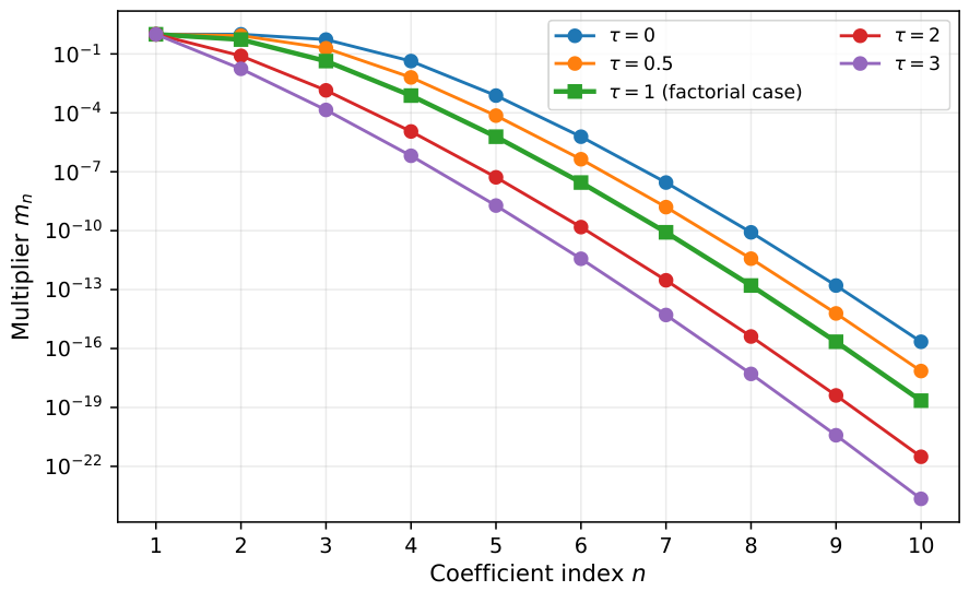
Figure 1 displays the multiplier $m_n(\kappa ,\ell ,\tau )$ for $n=1,\cdots ,10$, with $\kappa =1$, $\ell =1.5$, and several gamma shifts. The curve $\tau =1$ is emphasized because Equation (8) shows that it recovers the factorial Mathieu multiplier used in the closest earlier framework [26]. The remaining curves illustrate how the gamma deformation redistributes the coefficient suppression. Since both gamma factors in (6) vary with $\tau$, the displayed ordering is specific to these parameter values and is not asserted as a theorem in $\tau$.

• Active estimate and the degenerate set.

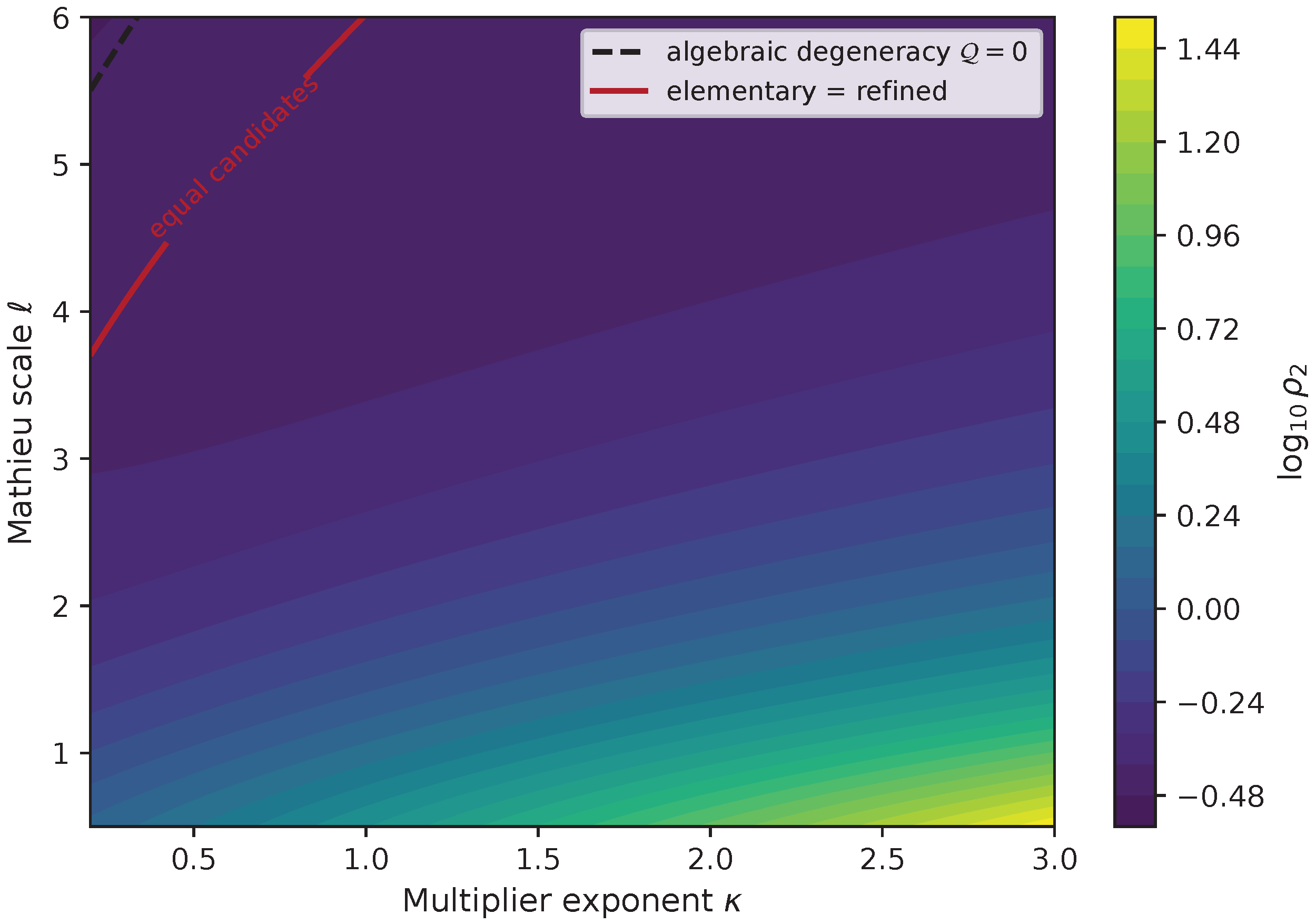
Figure 2 plots ${\log }_{10}{\rho }_2$ on $0.2\le \kappa \le 3$ and $0.5\le \ell \le 6$ for $\tau =1$, $\delta =1$, $\mu =\nu =\beta =0.5$, ${\rho }_{\mathrm{\Phi }}=0.2$, and ${\rho }_{\mathrm{\Psi }}=0.4$. The red contour is the branch-switching set $E=R$, whereas the dashed contour is the algebraically degenerate set $\mathcal{Q}=0$. The refined formula stays finite on the latter set, in agreement with Proposition 2.

• Combined operator and target sensitivity.

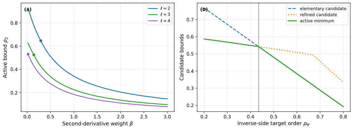
The two one-parameter experiments in Figure 3 expose the switching mechanism. Panel (a) varies $\beta$ for $\ell \in \{2,3,4\}$, with $\kappa =\tau =\delta =1$, $\mu =\nu =0.5$, ${\rho }_{\mathrm{\Phi }}=0.2$, and ${\rho }_{\mathrm{\Psi }}=0.6$. The marked transitions occur at $\beta \approx 0.2925$, $0.1439$, and $0.0213$, respectively. Panel (b) fixes $\kappa =0.2$, $\ell =8$, $\tau =\delta =1$, $\mu =\nu =0.5$, $\beta =0.05$, and ${\rho }_{\mathrm{\Phi }}=0.2$, while ${\rho }_{\mathrm{\Psi }}$ varies. The active candidate changes at ${\rho }_{\mathrm{\Psi }}\approx 0.4352$. This panel directly quantifies the effect of unequal function/inverse targets.

• Symmetric and asymmetric target geometry.

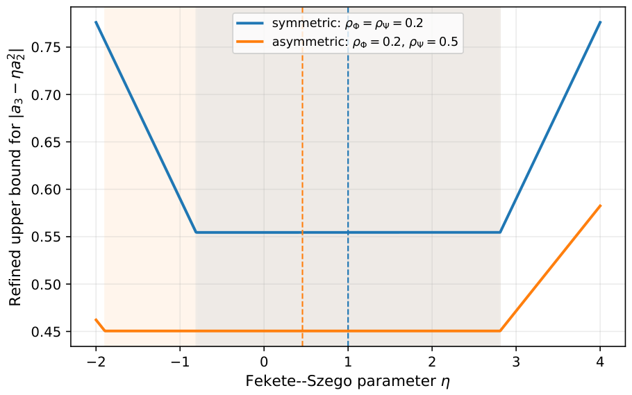
Figure 4 evaluates (40) for $-2\le \eta \le 4$ at $\kappa =\tau =\delta =1$, $\ell =4$, and $\mu =\nu =\beta =0.5$. For $\mathrm{\Phi }=\mathrm{\Psi }={\mathrm{\Phi }}_{0.2}$, the flat minimum is centered at $\eta =1$ and extends approximately over $[-0.8089,2.8089]$. For $\mathrm{\Phi }={\mathrm{\Phi }}_{0.2}$ and $\mathrm{\Psi }={\mathrm{\Phi }}_{0.5}$, the target-coefficient difference shifts the center to $\eta \approx 0.4573$ and the plateau to approximately $[-1.8943,2.8089]$. The plateau is a consequence of the term $\max \{0,|{\Lambda }_{\eta }|-D\}$ and was absent from the earlier estimate based only on $|u_2|,|v_2|\le 1$.

• Representative coefficient values and active branches.

Table 4. Representative coefficient estimates with their active branches.

$\mathit{\tau }$	$\mathit{\kappa }$	${\mathit{m}}_2$	${\mathit{m}}_3$	$\mathcal{Q}$	E	R	Active	${\mathit{\rho }}_2$	${\mathcal{B}}_3$
0	1	1.0000	1.4450	4.5050	0.4000	0.4471	elementary	0.4000	0.2215
0.5	1	1.3388	1.4445	−2.2346	0.2988	0.3913	elementary	0.2988	0.1846
1	1	1.4450	0.6413	−11.9768	0.2768	0.2947	elementary	0.2768	0.4158
1.5	1	1.0790	0.1207	−8.8096	0.3707	0.3699	refined	0.3699	2.2100
1	3	1.0440	0.0685	−8.6478	0.3831	0.3777	refined	0.3777	3.8908

fixes $\ell =4$, $\delta =1$, $\mu =\nu =\beta =0.5$, ${\rho }_{\mathrm{\Phi }}=0.2$, and ${\rho }_{\mathrm{\Psi }}=0.6$. The row $\tau =1$, $\kappa =1$ is the factorial model. The data show that the active estimate can be elementary or refined and that suppression of $m_3$ may enlarge the $|a_3|$ bound through reciprocal factors.

Table 5. Concise numerical summary of transition, gamma-shift, and target-asymmetry effects.

Effect	Fixed Setting	Numerical Diagnostic
Transition zones	Figure 3a, $\ell =2,3,4$	$E=R$ at $\beta \approx 0.2925,0.1439,0.0213$, respectively
Target-side transition	Figure 3b, ${\rho }_{\mathrm{\Phi }}=0.2$	Active branch switches at ${\rho }_{\mathrm{\Psi }}\approx 0.4352$
Gamma deformation	Table 4, $\kappa =1$	${\rho }_2=0.4000,0.2988,0.2768,0.3699$ for $\tau =0,0.5,1,1.5$; the dependence is not monotone
Target asymmetry	Figure 4	Fekete–Szegő center moves from 1 to $0.4573$ and the minimum bound decreases from $0.5545$ to $0.4505$

collects the three numerical effects requested for interpreting the parameter geometry.

These calculations confirm, but do not substitute for, the analytical results: $\tau$ really distorts the factorial coefficient; the effective estimator varies over non-empty parameter intervals; the new formulas are still bounded at $\mathcal{Q}=0$; and different targets change both branching and Fekete–Szegö geometry. No result beyond the displayed parameter intervals is implied.

10. Conclusions and Future Directions

This class is generated through the use of a gamma-deformed Mathieu multiplier and a two-sided generalized Ma–Minda condition for a function f that belongs to the family of bi-univalent functions. Exact second-order coefficient identities yield explicit bounds for $|a_2|$, $|a_3|$, and $|a_3-\eta a_2^2|$. The preservation of the Schwarz–Pick inequality in its entirety helps improve the quadratic $a_2$ and Fekete–Szegő inequalities; division by $\mathcal{Q}$ is not necessary in order to get the expressions right, thus allowing for cases where $\mathcal{Q}=0$. The study also yields inverse and logarithmic inequalities, target dominating containment, and direct inequalities for bounded turning, starlike, and convexity of the transform.

The numerical illustrations identify $\tau =1$ as the earlier factorial Mathieu model, display transitions between the elementary and refined $a_2$ candidates, locate the degenerate set, and quantify how unequal generalized targets shift the center and plateau of the refined Fekete–Szegő bound. The computations also clarify why stronger high-order multiplier suppression may enlarge a reciprocal coefficient estimate. These observations are restricted to the stated parameter domains and are not promoted to global monotonicity results.

The auxiliary Schwarz–Pick inequality is sharp and its equality cases are realized by degree-two Blaschke products. This does not establish simultaneous equality for the linked function- and inverse-side subordinations, so sharpness for the full bi-univalent class remains open. Further work should construct extremal functions for selected symmetric subclasses, establish nontrivial radius theorems, classify the geometry of $\mathcal{Q}=0$ and $E=R$, and derive genuinely higher-order Hankel estimates through third- and fourth-order coefficient comparisons.

References

- Lewin, M. On a coefficient problem for bi-univalent functions. Proc. Am. Math. Soc. 1967, 18, 63–68. [Google Scholar] [CrossRef]
- Brannan, D.A.; Taha, T.S. On some classes of bi-univalent functions. In Mathematical Analysis and Its Applications; Mazhar, S.M., Hamoui, A., Faour, N.S., Eds.; KFAS Proceedings Series; Pergamon Press: Oxford, UK, 1988; Volume 3, pp. 53–60. [Google Scholar] [CrossRef] [Scilit]
- Srivastava, H.M.; Mishra, A.K.; Gochhayat, P. Certain subclasses of analytic and bi-univalent functions. Appl. Math. Lett. 2010, 23, 1188–1192. [Google Scholar] [CrossRef] [Scilit]
- Duren, P.L. Univalent Functions; Grundlehren der Mathematischen Wissenschaften Series; Springer: New York, NY, USA, 1983; Volume 259. [Google Scholar]
- Ma, W.; Minda, D. A unified treatment of some special classes of univalent functions. In Proceedings of the Conference on Complex Analysis; International Press: Cambridge, MA, USA, 1994; pp. 157–169. [Google Scholar]
- Long, P.; Murugusundaramoorthy, G.; Tang, H.; Wang, W. Subclasses of analytic and bi-univalent functions involving a generalized Mittag-Leffler function based on quasi-subordination. J. Math. Comput. Sci. 2022, 26, 379–394. [Google Scholar] [CrossRef] [Scilit]
- Hussen, A.; Illafe, M. Coefficient bounds for a certain subclass of bi-univalent functions associated with Lucas-balancing polynomials. Mathematics 2023, 11, 4941. [Google Scholar] [CrossRef] [Scilit]
- Aldawish, I.; Sharma, P.; El-Deeb, S.M.; Almutairi, M.R.; Sivasubramanian, S. Initial coefficient bounds for certain new subclasses of bi-univalent functions involving Mittag-Leffler function with bounded boundary rotation. Symmetry 2024, 16, 971. [Google Scholar] [CrossRef] [Scilit]
- Illafe, M.; Mohd, M.H.; Yousef, F.; Supramaniam, S. Bounds for the second Hankel determinant of a general subclass of bi-univalent functions. Int. J. Math. Eng. Manag. Sci. 2024, 9, 1226–1239. [Google Scholar] [CrossRef] [Scilit]
- El-Ityan, M.; Sabri, M.A.; Hammad, S.; Frasin, B.; Al-Hawary, T.; Yousef, F. Third-order Hankel determinant for a class of bi-univalent functions associated with sine function. Mathematics 2025, 13, 2887. [Google Scholar] [CrossRef] [Scilit]
- Yousef, F.; Al-Hawary, T.; El-Ityan, M.; Aldawish, I. Novel bi-univalent subclasses generated by the q-analogue of the Ruscheweyh operator and Hermite polynomials. Mathematics 2026, 14, 382. [Google Scholar] [CrossRef] [Scilit]
- Fekete, M.; Szegő, G. Eine Bemerkung über ungerade schlichte Funktionen. J. Lond. Math. Soc. 1933, s1-8, 85–89. [Google Scholar] [CrossRef] [Scilit]
- Mathieu, E. Théorie de l’élasticité des Corps Solides; Gauthier-Villars: Paris, France, 1890. [Google Scholar]
- Emersleben, O. Über die Reihe . Math. Ann. 1952, 125, 165–171. [Google Scholar]
- Alzer, H.; Brenner, J.L.; Ruehr, O.G. On Mathieu’s inequality. J. Math. Anal. Appl. 1998, 218, 607–610. [Google Scholar] [CrossRef] [Scilit]
- Cerone, P.; Lenard, C.T. On integral forms of generalized Mathieu series. J. Inequal. Pure Appl. Math. 2003, 4, 100. [Google Scholar]
- Choi, J.; Srivastava, H.M. Mathieu series and associated sums involving the zeta functions. Comput. Math. Appl. 2010, 59, 861–867. [Google Scholar] [CrossRef] [Scilit]
- Tomovski, Z.; Pogány, T.K. Integral expressions for Mathieu-type power series and for the Butzer–Flocke–Hauss omega-function. Fract. Calc. Appl. Anal. 2011, 14, 623–634. [Google Scholar] [CrossRef] [Scilit]
- Srivastava, H.M.; Mehrez, K.; Tomovski, Z. New inequalities for some generalized Mathieu-type series and the Riemann zeta function. J. Math. Inequal. 2018, 12, 163–174. [Google Scholar] [CrossRef] [Scilit]
- Tomovski, Z.; Leskovski, D.; Gerhold, S. Generalized Mathieu Series; Springer: Cham, Switzerland, 2021. [Google Scholar]
- Bansal, D.; Sokół, J. Geometric properties of Mathieu-type power series inside the unit disk. J. Math. Inequal. 2019, 13, 911–918. [Google Scholar] [CrossRef] [Scilit]
- Gerhold, S.; Hubalek, F.; Tomovski, Z. Asymptotics of some generalized Mathieu series. Math. Scand. 2020, 126, 424–450. [Google Scholar] [CrossRef] [Scilit]
- Tomovski, Z.; Gerhold, S.; Bansal, D.; Soni, A. Geometric properties of some generalized Mathieu power series inside the unit disk. Axioms 2022, 11, 568. [Google Scholar] [CrossRef] [Scilit]
- Liu, D.; Araci, S.; Khan, B. A subclass of Janowski starlike functions involving Mathieu-type series. Symmetry 2022, 14, 2. [Google Scholar] [CrossRef] [Scilit]
- Oyekan, E.A.; Opoola, T.O. On a set of generalized Janowski-type starlike functions connected with Mathieu-type series and Opoola differential operator. Pan-Am. J. Math. 2023, 2, 11. [Google Scholar] [CrossRef] [Scilit]
- Yousef, F.; Al-Hawary, T.; Alhindi, K.R.; Obiedat, H. Coefficient estimates for analytic and bi-univalent functions classes defined by generalized Mathieu-type power series. Mathematics 2026, 14, 1822. [Google Scholar] [CrossRef] [Scilit]