A Two-Way Convolution of the Mittag-Leffler Function with Sheffer Polynomials

Abstract

This article presents a two-way convolution of the Mittag-Leffler function with Sheffer polynomials via the umbral algebraic method, thereby introducing the Mittag-Leffler–Sheffer polynomials (MLSPs) and the Sheffer–Mittag-Leffler function (SMLF). We establish their generating functions, series definitions, quasi-monomial properties, and differential equations. Using Wronskian and Pascal functional matrices, we derive recursive formulas and differential recursive identities for these hybrid polynomials. Various special cases including Mittag-Leffler–Appell, Mittag-Leffler–Hermite, and Mittag-Leffler–Miller–Lee polynomials are examined. Additionally, a graphical investigation of the zero distributions of selected members of these polynomial families is presented using computational tools.

1. Introduction and Preliminaries

The umbral algebraic approach provides a powerful framework for analyzing the characteristics of Sheffer and Appell polynomials through Pascal functional and Wronskian matrices. Working entirely within matrix operations, this method yields a self-contained theory for deriving recursive formulas and differential equations for hybrid families of polynomials, as developed in [1,2]. The technique proves especially effective for investigating generalized hybrid-type special polynomials. In particular, the derivation of recursive identities and differential recursive identities for Sheffer polynomials relies on the application of Wronskian and Pascal functional matrices.

We recall the basic matrix definitions that serve as the foundation for deriving the results presented in Section 3 and Section 4.

Let ${\displaystyle \mathcal{H}=\left\{{\displaystyle \sum _{k=0}^{\infty }}{a}_k\frac{t^k}{k!}:a_k\in \mathbb{C}\right\}}$ be the $\mathbb{C}$-algebra of formal power series. For $p\left(t\right)\in \mathcal{H}$, the generalized Pascal functional matrix [3] of an analytic function $p\left(t\right)$, denoted by ${\mathcal{F}}_n\left[p\left(t\right)\right]$ is a square matrix of order $n+1$ defined as

$${\left({\mathcal{F}}_n\left[p\left(t\right)\right]\right)}_{m,k}=\left\{\begin{array}{cc}\left({\displaystyle \genfrac{}{}{0pt}{}{m}{k}}\right)p^{(m-k)}\left(t\right),\hfill & \mathrm{if}m\ge k,m,k=0,1,2,\dots ,n,\hfill \\ 0,\hfill & \mathrm{otherwise}.\hfill \end{array}\right.$$

(1)

It should be noted that $p^{\left(m\right)}$ denotes the m-th order derivative of p, and $p^m$ denotes the m-th power of p throughout the article. The notation $p^{-1}\left(t\right)$ denotes the compositional inverse of $p\left(t\right)$, i.e., the unique formal power series satisfying $p\left(p^{-1}\left(t\right)\right)=t$; it does not denote the reciprocal $1/p\left(t\right)$.

For any analytic functions $p_1\left(t\right),p_2\left(t\right),\dots ,p_m\left(t\right)$, the n-th order Wronskian matrix is a matrix of order $(n+1)\times m$ and is defined as

$${\mathcal{W}}_n[p_1\left(t\right),p_2\left(t\right),\dots ,p_m\left(t\right)]=\left(\begin{array}{cccc}{p}_1\left(t\right)& p_2\left(t\right)& \dots & p_m\left(t\right)\\ p_1^{\prime }\left(t\right)& p_2^{\prime }\left(t\right)& \dots & p_m^{\prime }\left(t\right)\\ ⋮& ⋮& \ddots & ⋮\\ p_1^{\left(n\right)}\left(t\right)& p_2^{\left(n\right)}\left(t\right)& \dots & p_m^{\left(n\right)}\left(t\right)\end{array}\right).$$

(2)

For any scalars $a,b\in \mathbb{C}$ and analytic functions $p\left(t\right)$, $q\left(t\right)\in \mathcal{H}$, the Pascal functional and Wronskian matrices [2] satisfy the following relations:

$$\begin{array}{cc}\hfill {\mathcal{F}}_n[ap\left(t\right)+bq\left(t\right)]& =a{\mathcal{F}}_n\left[p\left(t\right)\right]+b{\mathcal{F}}_n\left[q\left(t\right)\right],\hfill \end{array}$$

(3)

$$\begin{array}{cc}\hfill {\mathcal{W}}_n[ap\left(t\right)+bq\left(t\right)]& =a{\mathcal{W}}_n\left[p\left(t\right)\right]+b{\mathcal{W}}_n\left[q\left(t\right)\right],\hfill \end{array}$$

(4)

$$\begin{array}{cc}\hfill {\mathcal{F}}_n\left[p\left(t\right)\right]{\mathcal{F}}_n\left[q\left(t\right)\right]& ={\mathcal{F}}_n\left[q\left(t\right)\right]{\mathcal{F}}_n\left[p\left(t\right)\right]={\mathcal{F}}_n\left[p(⌀)q\left(t\right)\right],\hfill \end{array}$$

(5)

$$\begin{array}{cc}\hfill {\mathcal{F}}_n\left[p\left(t\right)\right]{\mathcal{W}}_n\left[q\left(t\right)\right]& ={\mathcal{F}}_n\left[q\left(t\right)\right]{\mathcal{W}}_n\left[p\left(t\right)\right]={\mathcal{W}}_n\left[\left(pq\right)\left(t\right)\right],\hfill \end{array}$$

(6)

and

$${\mathcal{W}}_n{\left[q\left(p\left(t\right)\right)\right]}_{t=0}={\mathcal{W}}_n{[1,p\left(t\right),p^2\left(t\right),\dots ,p^n\left(t\right)]}_{t=0}{\mathsf{\Lambda }}_n^{-1}{\mathcal{W}}_n{\left[q\left(t\right)\right]}_{t=0},$$

(7)

where ${\mathsf{\Lambda }}_n=\mathrm{diag}[0!,1!,2!,\dots ,n!]$, $p\left(0\right)=0$ and $p^{\prime }\left(0\right)\ne 0$.

Further, for any analytic functions $p_1\left(t\right),p_2\left(t\right),\dots ,p_m\left(t\right)$ and $q\left(t\right)$,

$${\mathcal{F}}_n\left[q\left(t\right)\right]{\mathcal{W}}_n[p_1\left(t\right),p_2\left(t\right),\dots ,p_m\left(t\right)]={\mathcal{W}}_n[\left(q{p}_1\right)\left(t\right),\left(q{p}_2\right)\left(t\right),\dots ,\left(q{p}_m\right)\left(t\right)].$$

(8)

The sequences of polynomials play a significant role in several branches of mathematics. One of the important class of polynomial sequences is the class of Sheffer sequences [4]. Sheffer sequences are used to solve numerous problems in applied mathematics, theoretical physics, approximation theory, and several other mathematical fields. According to Roman [4], the Sheffer polynomials $s_n\left(x\right)$ are uniquely determined by two (formal) power series, $p\left(t\right)$ and $q\left(t\right)$,

$$p\left(t\right)={\displaystyle \sum _{n=0}^{\infty }}{p}_n{\displaystyle \frac{t^n}{n!}},p_0=0,p_1\ne 0,$$

(9)

$$q\left(t\right)={\displaystyle \sum _{n=0}^{\infty }}{q}_n{\displaystyle \frac{t^n}{n!}},q_0\ne 0.$$

(10)

Then, the generating function for $s_n\left(x\right)$ is given by [5]

$${\displaystyle \sum _{n=0}^{\infty }}{s}_n\left(x\right){\displaystyle \frac{t^n}{n!}}={\displaystyle \frac{e^{x{p}^{-1}\left(t\right)}}{q\left(p^{-1}\left(t\right)\right)}},x\in \mathbb{C},$$

(11)

When $p\left(t\right)=t$, these reduce to the Appell polynomials $A_n\left(x\right)$ [6], whose extended forms via fractional operators and determinant representations have been studied in [7]. The generating function is given by

$${\displaystyle \sum _{n=0}^{\infty }}{A}_n\left(x\right){\displaystyle \frac{t^n}{n!}}={\displaystyle \frac{e^{xt}}{q\left(t\right)}}.$$

(12)

If $s_n\left(x\right)$ admits the following generating function, it is called Sheffer-type [8]:

$${\displaystyle \sum _{n=0}^{\infty }}{s}_n\left(x\right){\displaystyle \frac{t^n}{n!}}=\mathcal{A}\left(t\right)e^{xH\left(t\right)},x\in \mathbb{C},$$

(13)

where $\mathcal{A}\left(t\right)$ and $H\left(t\right)$ have formal expansions

$$\mathcal{A}\left(t\right)={\displaystyle \sum _{n=0}^{\infty }}{\mathcal{A}}_n{\displaystyle \frac{t^n}{n!}},{\mathcal{A}}_0\ne 0,$$

(14)

and

$$H\left(t\right)={\displaystyle \sum _{n=1}^{\infty }}{H}_n{\displaystyle \frac{t^n}{n!}},H_1\ne 0,$$

(15)

respectively. From Equations (11) and (13), we obtain

$$\mathcal{A}\left(t\right)={\displaystyle \frac{1}{q\left(p^{-1}\left(t\right)\right)}},$$

(16)

and

$$H\left(t\right)=p^{-1}\left(t\right).$$

(17)

The umbral image for Sheffer polynomials [9] is given by

$$s_n\left(x\right)={(x\widehat{h}+\widehat{a})}^n{\varphi }_0{\phi }_0,$$

(18)

where $\widehat{a}$ and $\widehat{h}$ are umbral operators acting on vacuum functions ${\varphi }_0$ and ${\phi }_0$ respectively. Moreover, in [9] is stated:

$$\begin{array}{cc}\hfill \mathcal{A}\left(t\right)& =e^{\widehat{a}t}{\varphi }_0,\hfill \end{array}$$

(19)

$$\begin{array}{cc}\hfill H\left(t\right)& =\widehat{h}t{\phi }_0.\hfill \end{array}$$

(20)

The series definition for the two-parameter Mittag-Leffler function (2pMLF) is given by [10,11]

$$E_{\alpha ,\beta }\left(x\right)={\displaystyle \sum _{r=0}^{\infty }}{\displaystyle \frac{x^r}{\mathsf{\Gamma }(\alpha r+\beta )}},\forall x\in \mathbb{R},\forall \alpha ,\beta \in {\mathbb{R}}^{+}.$$

(21)

Dattoli et al. [12] introduced symbolic definition of the two-parameter Mittag-Leffler function as

$$E_{\alpha ,\beta }\left(x\right)=e^{x{\widehat{d}}_{(\alpha ,\beta )}}{\psi }_0,$$

(22)

where ${\widehat{d}}_{(\alpha ,\beta )}$   $(\alpha ,\beta \in \mathbb{R})$ denotes a symbolic operator, which operates on the vacuum function

$${\displaystyle {\psi }_z=\frac{\mathsf{\Gamma }(z+1)}{\mathsf{\Gamma }(\alpha z+\beta )}}$$

as

$${\displaystyle {\widehat{d}}_{(\alpha ,\beta )}^k{\psi }_z=\frac{\mathsf{\Gamma }(k+z+1)}{\mathsf{\Gamma }\left(\alpha (k+z)+\beta \right)},k\in \mathbb{R},k+z\ge -1.}$$

(23)

In particular, we have [13]

$${\displaystyle {\widehat{d}}_{(\alpha ,\beta )}^k{\psi }_0:={\left.{\widehat{d}}_{(\alpha ,\beta )}^k{\psi }_z\right|}_{z=0}=\frac{\mathsf{\Gamma }(k+1)}{\mathsf{\Gamma }(\alpha k+\beta )},k\in \mathbb{R},k\ge -1.}$$

(24)

Thus, in view of Equations (23) and (24), ${\widehat{d}}_{(\alpha ,\beta )}$ satisfies the property

$${\displaystyle {\widehat{d}}_{(\alpha ,\beta )}^k{\widehat{d}}_{(\alpha ,\beta )}^r{\psi }_0=\frac{\mathsf{\Gamma }(k+r+1)}{\mathsf{\Gamma }\left(\alpha (k+r)+\beta \right)},k,r\in \mathbb{R},k+r\ge -1.}$$

(25)

From Equation (24), it follows that

$${\widehat{d}}_{(\alpha ,\beta )}^{-1}{\psi }_0={\displaystyle \frac{1}{\mathsf{\Gamma }(\beta -\alpha )}}.$$

(26)

Evidently, for $k=0$, Equation (24) gives

$${\psi }_0={\displaystyle \frac{1}{\mathsf{\Gamma }\left(\beta \right)}}.$$

Differential and integral equations associated with Appell-type polynomial families have been systematically developed in [14], offering a framework that complements the operational approach employed here. The concept of monomiality, rooted in Steffensen’s poweroid abstraction [15], was reformulated by Dattoli [16]. A polynomial sequence ${\left\{S_n\left(x\right)\right\}}_{n=0}^{\infty }$ satisfies the quasi-monomial property under a multiplicative operator $\widehat{M}$ and a derivative operator $\widehat{P}$ if

$$\begin{array}{cc}\hfill \widehat{M}\left\{S_n\left(x\right)\right\}& =S_{n+1}\left(x\right),\hfill \end{array}$$

(27)

$$\begin{array}{cc}\hfill \widehat{P}\left\{S_n\left(x\right)\right\}& =n{S}_{n-1}\left(x\right),\hfill \end{array}$$

(28)

with the Weyl commutation relation

$$[\widehat{P},\widehat{M}]=\widehat{P}\widehat{M}-\widehat{M}\widehat{P}=\widehat{1}.$$

(29)

If a differential realization is available, we obtain

$$\widehat{M}\widehat{P}\left\{S_n\left(x\right)\right\}=n{S}_n\left(x\right),$$

(30)

and the polynomials can be expressed as

$$S_n\left(x\right)={\widehat{M}}^n\left\{S_0\left(x\right)\right\}.$$

(31)

The main contributions of this work are as follows. We construct a two-way umbral convolution between the Mittag-Leffler function and Sheffer polynomial sequences, yielding two new objects: the Mittag-Leffler Sheffer polynomials (MLSPs) and the Sheffer-Mittag-Leffler function (MLSP). The framework unifies these two separately studied structures through a common umbral calculus and yields generating functions, series representations, quasi-monomial operators, and differential equations within a single formalism. Wronskian and Pascal functional matrices are used to derive recursive and differential recursive identities, extending the matrix-algebraic techniques of [1,2] to the fractional-function setting. The special cases Mittag-Leffler-Appell, Mittag-Leffler-Hermite, and Mittag-Leffler-Miller-Lee polynomials—show how the framework unifies several existing polynomial families, and the structural asymmetry between MLSPs and SMLFs opens directions for further study.

The remainder of this paper is organized as follows. Section 2 introduces the Mittag-Leffler–Sheffer polynomials and establishes their generating function, series representation (Theorem 1), quasi-monomial operators (Theorem 2), differential equation (Theorem 3), higher-order derivative formula (Theorem 4), and operational rule (Theorem 5). Section 3 derives recursive formulas for the MLSP via the Wronskian and Pascal matrix approach, yielding a vector identity (Theorem 6) and both differential (Theorem 7) and pure (Theorems 8 and 9) recursive identities. Section 4 establishes differential equation formulas for the MLSP, including a general differential equation (Theorem 10) and a differential identity connecting polynomials of successive degrees (Theorem 11). Section 5 presents summation formulae and integral representations, comprising an addition formula (Theorem 12), a multiplication formula (Theorem 13), an integral representation (Theorem 14), and a connection formula between different parameter pairs (Theorem 15). Section 6 specializes the general results to three concrete families-Mittag-Leffler-Appell, Mittag-Leffler-Hermite, and Mittag-Leffler-Miller-Lee polynomials with explicit recursive and differential identities for each. The graphical investigation of the zero distributions of selected polynomial families is carried out in Section 7. Section 8 introduces the Sheffer-Mittag-Leffler function and outlines directions for further research.

2. Mittag-Leffler–Sheffer Polynomials

In this section, we introduce the Mittag-Leffler–Sheffer polynomials (MLSPs)_E $s_n^{(\alpha ,\beta )}\left(x\right)$ with the help of umbral image. Also, we derive series definition, quasi monomiality property, differential equation, partial derivatives and operational rules. We start with the following definition as

The Mittag-Leffler–Sheffer polynomials ${}_{E}s_n^{(\alpha ,\beta )}\left(x\right)$ are defined by means of the following generating function as

$${\displaystyle \sum _{n=0}^{\infty }}{}_{E}s_n^{(\alpha ,\beta )}\left(x\right){\displaystyle \frac{t^n}{n!}}=\mathcal{A}\left(t\right)E_{\alpha ,\beta }\left(xH\left(t\right)\right),$$

(32)

or equivalently,

$${\displaystyle \sum _{n=0}^{\infty }}{}_{E}s_n^{(\alpha ,\beta )}\left(x\right){\displaystyle \frac{t^n}{n!}}={\displaystyle \frac{1}{q\left(p^{-1}\left(t\right)\right)}}{E}_{\alpha ,\beta }\left(xH\left(t\right)\right).$$

(33)

By using Equations (18) and (22) in Equation (32), we get the following symbolic definition of Mittag-Leffler–Sheffer polynomials (MLSPs) ${}_{E}s_n^{(\alpha ,\beta )}\left(x\right)$:

$${\displaystyle \sum _{n=0}^{\infty }}{}_{E}s_n^{(\alpha ,\beta )}\left(x\right){\displaystyle \frac{t^n}{n!}}=e^{\left(x{\widehat{d}}_{(\alpha ,\beta )}\widehat{h}+\widehat{a}\right)t}{\psi }_0{\phi }_0{\varphi }_0.$$

(34)

We note that

$${}_{E}s_n^{(\alpha ,\beta )}\left(x\right)={(x{\widehat{d}}_{(\alpha ,\beta )}\widehat{h}+\widehat{a})}^n{\varphi }_0{\phi }_0{\psi }_0,$$

(35)

where ${\varphi }_0$ acts on $\widehat{a}$, ${\phi }_0$ acts on $\widehat{h}$, and ${\psi }_0$ acts on ${\widehat{d}}_{(\alpha ,\beta )}$.

The generating function approach adopted here parallels techniques used for multidimensional q-Hermite polynomials [17], where similar convolution structures arise in the context of quantum deformations.

Series expansions of this type have appeared in the study of generalized degenerate forms of two-dimensional Appell polynomials via fractional operators [18,19,20], which motivates our derivation below.

Theorem 1. 

The following series expansion holds true for the MLSP ${}_{E}s_n^{(\alpha ,\beta )}\left(x\right)$:

$${}_{E}s_n^{(\alpha ,\beta )}\left(x\right)={\displaystyle \sum _{k=0}^n}\left({\displaystyle \genfrac{}{}{0pt}{}{n}{k}}\right)x^k{\displaystyle \frac{\mathsf{\Gamma }(k+1)}{\mathsf{\Gamma }(\alpha k+\beta )}}{\mathcal{A}}_{n-k}{\widehat{h}}^k{\phi }_0.$$

(36)

Proof. 

Expanding the right-hand side of (34) by the binomial theorem gives

$${}_{E}s_n^{(\alpha ,\beta )}\left(x\right)={\displaystyle \sum _{k=0}^n}\left({\displaystyle \genfrac{}{}{0pt}{}{n}{k}}\right){\left(x{\widehat{d}}_{(\alpha ,\beta )}\widehat{h}\right)}^k{\widehat{a}}^{n-k}{\varphi }_0{\psi }_0{\phi }_0.$$

Employing Equation (24) in the preceding equation, it follows that

$${}_{E}s_n^{(\alpha ,\beta )}\left(x\right)={\displaystyle \sum _{k=0}^n}\left({\displaystyle \genfrac{}{}{0pt}{}{n}{k}}\right){\rho }^k{\displaystyle \frac{\mathsf{\Gamma }(k+1)}{\mathsf{\Gamma }(\alpha k+\beta )}}{\widehat{h}}_k{\widehat{a}}_{n-k}{\phi }_0{\varphi }_0,$$

therefore on using Equations (14) and (19) in the above equation, yields the assertion (36).    □

Theorem 2. 

The quasi-monomiality property with respect to the following multiplicative and derivative operators for Mittag-Leffler–Sheffer polynomials ${}_{E}s_n^{(\alpha ,\beta )}\left(x\right)$ hold true:

$${\widehat{M}}_{{}_{E}s}=x{\widehat{d}}_{(\alpha ,\beta )}\widehat{h}+\widehat{a},$$

(37)

and

$${\widehat{P}}_{{}_{E}s}={\widehat{d}}_{(\alpha ,\beta )}^{-1}{\widehat{h}}^{-1}{D}_x,$$

(38)

respectively.

Proof. 

Operating $(x{\widehat{d}}_{(\alpha ,\beta )}\widehat{h}+\widehat{a})$ on both sides of Equation (34) and using (34) again in the resulting expression, one obtains

$$(x{\widehat{d}}_{(\alpha ,\beta )}\widehat{h}+\widehat{a}){}_{E}s_n^{(\alpha ,\beta )}\left(x\right)={}_{E}s_{n+1}^{(\alpha ,\beta )}\left(x\right).$$

This, in view of Equation (27), yields the assertion (37).

Differentiating Equation (34) with respect to x and applying (34) gives

$${\displaystyle \frac{\partial }{\partial x}}{}_{E}s_n^{(\alpha ,\beta )}\left(x\right)=n{\widehat{d}}_{(\alpha ,\beta )}\widehat{h}{}_{E}s_{n-1}^{(\alpha ,\beta )}\left(x\right).$$

(39)

In light of Equations (28) and (39), we obtain the assertion (38).    □

Theorem 3. 

The following differential equation holds true for the MLSP:

$$\left[(x{\widehat{d}}_{(\alpha ,\beta )}+\widehat{a}){\widehat{d}}_{(\alpha ,\beta )}^{-1}{\widehat{h}}^{-1}{\displaystyle \frac{\partial }{\partial x}}-n\right]{}_{E}s_n^{(\alpha ,\beta )}\left(x\right)=0.$$

(40)

Proof. 

This follows directly from Equations (30), (37) and (38).    □

Theorem 4. 

The higher-order partial derivatives of the MLSP satisfy:

$$D_x^s{}_{E}s_n^{(\alpha ,\beta )}\left(x\right)={\displaystyle \frac{n!}{(n-s)!}}{\widehat{d}}_{(\alpha ,\beta )}^s{\widehat{h}}^s{}_{E}s_{n-s}^{(\alpha ,\beta )}\left(x\right),$$

(41)

with initial condition

$${}_{E}s_n^{(\alpha ,\beta )}\left(0\right)={\displaystyle \frac{{\mathcal{A}}_n}{\mathsf{\Gamma }\left(\beta \right)}}.$$

(42)

Proof. 

Carrying out mathematical induction by s, from (39). Assuming it holds for $s=k$ and differentiating once more with respect to x gives the case $s=k+1$, establishing the result by induction. Setting $x=0$ in (36) and using (26) yields the initial condition (42).    □

Theorem 5. 

The MLSP satisfies the following operational rule:

$${}_{E}s_n^{(\alpha ,\beta )}\left(x\right)=e^{x{\widehat{d}}_{(\alpha ,\beta )}\widehat{h}{D}_x}\left\{{\mathcal{A}}_n{\psi }_0\right\}.$$

(43)

Proof. 

The formal solution of the differential equation

$${\displaystyle \frac{\partial }{\partial x}}{}_{E}s_n^{(\alpha ,\beta )}\left(x\right)={\widehat{d}}_{(\alpha ,\beta )}\widehat{h}{D}_x{}_{E}s_n^{(\alpha ,\beta )}\left(x\right),$$

subject to the initial condition (42), is given by the action of the exponential operator $e^{x{\widehat{d}}_{(\alpha ,\beta )}\widehat{h}{D}_x}$ on the initial data. In view of the Crofton identity [16]

$$e^{\lambda D_x^m}\left\{f\left(x\right)\right\}=f(x+m\lambda D_x^{m-1})e^{\lambda D_x^m},$$

(44)

the operational action produces the assertion (43).    □

3. Recursive Formulas

In this section, we establish recursive formulae for the Mittag-Leffler–Sheffer polynomials ${}_{E}s_n^{(\alpha ,\beta )}\left(x\right)$ using Pascal and Wronskian matrices. To do this, we require the vector form of these polynomials.

The Mittag-Leffler–Sheffer vectors ${\overline{{}_{E}s}}_n^{(\alpha ,\beta )}\left(x\right)$ is defined by

$${\overline{{}_{E}s}}_n^{(\alpha ,\beta )}\left(x\right)={[{}_{E}s_0^{(\alpha ,\beta )}\left(x\right){}_{E}s_1^{(\alpha ,\beta )}\left(x\right){}_{E}s_2^{(\alpha ,\beta )}\left(x\right)\dots {}_{E}s_n^{(\alpha ,\beta )}\left(x\right)]}^T.$$

(45)

Since ${\displaystyle \frac{1}{q\left(p^{-1}\left(t\right)\right)}}{e}^{\left(x{\widehat{d}}_{(\alpha ,\beta )}\right)\widehat{h}t}{\phi }_0{\psi }_0$ is analytic, by Taylor’s series we have

$${}_{E}s_k^{(\alpha ,\beta )}\left(x\right)={\left({\displaystyle \frac{d}{dt}}\right)}^k{\displaystyle \frac{e^{\left(x{\widehat{d}}_{(\alpha ,\beta )}\right))\widehat{h}t}}{q\left(p^{-1}\left(t\right)\right)}}{\phi }_0{\psi }_0{|}_{t=0},k\ge 0,$$

(46)

which can be written as

$${\overline{{}_{E}s}}_n^{(\alpha ,\beta )}\left(x\right)={\mathcal{W}}_n{\left[{\displaystyle \frac{e^{\left(x{\widehat{d}}_{(\alpha ,\beta )}\right)\widehat{h}t}}{q\left(p^{-1}\left(t\right)\right)}}{\phi }_0{\psi }_0\right]}_{t=0}.$$

(47)

Theorem 6. 

The MLSP satisfies the following vector identity:

$$\begin{array}{c}{\left({\mathcal{W}}_n[{}_{E}s_0^{(\alpha ,\beta )}\left(x\right){}_{E}s_1^{(\alpha ,\beta )}\left(x\right)\dots {}_{E}s_n^{(\alpha ,\beta )}\left(x\right)]\right)}^T{\mathsf{\Lambda }}_n^{-1}\hfill \\ \hfill ={\mathcal{W}}_n{\left[1,p^{-1}\left(t\right),{\left(p^{-1}\left(t\right)\right)}^2,\dots ,{\left(p^{-1}\left(t\right)\right)}^n\right]}_{t=0}{\mathsf{\Lambda }}_n^{-1}{\mathcal{F}}_n{\left[{\displaystyle \frac{E_{\alpha ,\beta }\left(xH\left(t\right)\right)}{q\left(t\right)}}\right]}_{t=0}.\end{array}$$

(48)

Proof. 

Substituting Equation (7) in the right-hand side of Equation (47) and using ${\mathcal{W}}_n{\left[e^{xt}\right]}_{t=0}={[1x{x}^2\dots x^n]}^T$ together with Equations (6) and (22), one obtains the assertion by differentiating k times with respect to x, dividing by $k!$, and identifying columns of the resulting matrix equations. □

Theorem 7. 

The MLSP satisfies the following differential recursive formula:

$${}_{E}s_{n+1}^{(\alpha ,\beta )}\left(x\right)={\displaystyle \sum _{k=0}^n}{\displaystyle \frac{x{\widehat{d}}_{(\alpha ,\beta )}\widehat{h}+{\gamma }_k}{k!}}{D}_x^k{}_{E}s_n^{(\alpha ,\beta )}\left(x\right),$$

(49)

where ${}_{E}s_0^{(\alpha ,\beta )}\left(x\right)={\displaystyle \frac{1}{q\left(0\right)}}$ and ${\displaystyle {\gamma }_k={\left.{\left(-\frac{q^{\prime }\left(t\right)}{q\left(t\right)p^{\prime }\left(t\right)}\right)}^{\left(k\right)}\right|}_{t=0}}$.

Proof. 

Differentiating Equation (47) with respect to t and applying Equations (6) and (7), and the vector identity (48), and comparing the last rows of the resulting matrix equations yields the assertion.    □

Theorem 8. 

The following pure recursive formula holds for the MLSP:

$${\delta }_0{}_{E}s_{n+1}^{(\alpha ,\beta )}\left(x\right)={\displaystyle \sum _{k=0}^n}\left({\displaystyle \genfrac{}{}{0pt}{}{n}{k}}\right)(x{\widehat{d}}_{(\alpha ,\beta )}\widehat{h}{\delta }_k+{\zeta }_k){}_{E}s_n^{(\alpha ,\beta )}\left(x\right)-{\displaystyle \sum _{k=1}^n}\left({\displaystyle \genfrac{}{}{0pt}{}{n}{k}}\right){\delta }_k{}_{E}s_n^{(\alpha ,\beta )}\left(x\right),$$

(50)

where ${\delta }_k={\left(p^{\prime }\left(p^{-1}\left(t\right)\right)\right)}^{\left(k\right)}{|}_{t=0}$ and ${\displaystyle {\zeta }_k={\left.{\left(-\frac{q^{\prime }\left(p^{-1}\left(t\right)\right)}{q\left(p^{-1}\left(t\right)\right)}\right)}^{\left(k\right)}\right|}_{t=0}}$.

Proof. 

Using Equation (6) in the expression ${\displaystyle {\mathcal{W}}_n{\left[p^{\prime }\left(p^{-1}\left(t\right)\right)\frac{d}{dt}\left(\frac{e^{\left(x{\widehat{d}}_{(\alpha ,\beta )}\right)\widehat{h}t}}{q\left(p^{-1}\left(t\right)\right)}{\phi }_0{\psi }_0\right)\right]}_{t=0}}$ and applying Equations (46), (5), and (6) and then comparing the last rows of the resulting matrix equations yields the assertion.    □

Theorem 9. 

The MLSP satisfies the following pure recursive formula:

$${}_{E}s_{n+1}^{(\alpha ,\beta )}\left(x\right)={\displaystyle \sum _{k=0}^n}\left({\displaystyle \genfrac{}{}{0pt}{}{n}{k}}\right)(x{\widehat{d}}_{(\alpha ,\beta )}\widehat{h}+{\mho }_k){}_{E}s_{n-k}^{(\alpha ,\beta )}\left(x\right),$$

(51)

where ${\displaystyle {\mho }_k={\left.{\left(-\frac{q^{\prime }\left(p^{-1}\left(t\right)\right)}{q\left(p^{-1}\left(t\right)\right)p^{\prime }\left(p^{-1}\left(t\right)\right)}\right)}^{\left(k\right)}\right|}_{t=0}}$.

Proof. 

Differentiating the expression ${\displaystyle {\mathcal{W}}_n{\left[\frac{d}{dt}\left(\frac{e^{\left(x{\widehat{d}}_{(\alpha ,\beta )}\right)\widehat{h}t}}{q\left(p^{-1}\left(t\right)\right)}{\phi }_0{\psi }_0\right)\right]}_{t=0}}$ and using Equations (5), (6) and (48), then comparing the last rows yields the assertion.    □

4. Recursive Differential Equation Formulas

In this section, we derive differential equations for the MLSP using the matrix approach. The interplay between fractional calculus and generalized forms of special polynomials associated with Appell sequences has been explored in [21], providing additional context for the differential identities obtained below.

Theorem 10. 

The following differential equation holds for the MLSP:

$${\displaystyle \sum _{k=1}^n}{\displaystyle \frac{x{\widehat{d}}_{(\alpha ,\beta )}\widehat{h}{\nu }_k+{\theta }_k}{k!}}{D}_x^k{}_{E}s_n^{(\alpha ,\beta )}\left(x\right)-n{}_{E}s_n^{(\alpha ,\beta )}\left(x\right)=0,$$

(52)

where ${\nu }_k={\left(p\left(t\right)\right)}^{\left(k\right)}{|}_{t=0}$ and ${\displaystyle {\theta }_k={\left.{\left(-\frac{q^{\prime }\left(t\right)p\left(t\right)}{q\left(t\right)p^{\prime }\left(t\right)}\right)}^{\left(k\right)}\right|}_{t=0}}$.

Proof. 

Using Equation (6) in the expression ${\displaystyle {\mathcal{W}}_n{\left[t\frac{d}{dt}\left(\frac{e^{\left(x{\widehat{d}}_{(\alpha ,\beta )}\right)\widehat{h}t}}{q\left(p^{-1}\left(t\right)\right)}{\phi }_0{\psi }_0\right)\right]}_{t=0}}$, we evaluate this in two ways. On one hand, using ${\mathcal{F}}_n{\left[t\right]}_{t=0}$ with Equations (5), (6) and (46), we obtain a matrix involving the subdiagonal shift operator acting on the polynomial vector. On the other hand, differentiating directly and using Equation (7) followed by (48), we arrive at a matrix involving the Pascal matrix of derivatives of the polynomials. Comparing the last rows of these two expressions yields the assertion (52).    □

Theorem 11. 

The MLSP satisfies the following differential identity:

$${}_{E}s_n^{(\alpha ,\beta )}\left(x\right)={\displaystyle \frac{1}{n+1}}{\displaystyle \sum _{k=1}^{n+1}}{\displaystyle \frac{{\varrho }_k}{k!}}{D}_x^k{}_{E}s_{n+1}^{(\alpha ,\beta )}\left(x\right),$$

(53)

where ${\varrho }_k=p^{\left(k\right)}\left(0\right)$.

Proof. 

Using Equation (6) in the expression ${\displaystyle {\mathcal{W}}_n{\left[t\left(\frac{e^{\left(x{\widehat{d}}_{(\alpha ,\beta )}\right)\widehat{h}t}}{q\left(p^{-1}\left(t\right)\right)}{\phi }_0{\psi }_0\right)\right]}_{t=0}}$, evaluating in two ways via ${\mathcal{F}}_n{\left[t\right]}_{t=0}$ and via Equation (7) with (48), then comparing entries of the n-th rows and replacing $n\to n+1$ yields the assertion (53).    □

5. Summation Formulae and Integral Representations

In this section, we derive several summation formulae and integral representations for the MLSP. Analogous summation results for degenerate two-dimensional bivariate Appell polynomials have been established in [22], and the techniques therein are adapted to the Mittag-Leffler setting.

Theorem 12. 

The following summation formula holds for the MLSP:

$${}_{E}s_n^{(\alpha ,\beta )}(x+\sigma )={\displaystyle \sum _{k=0}^n}\left({\displaystyle \genfrac{}{}{0pt}{}{n}{k}}\right){\sigma }^k{\widehat{d}}_{(\alpha ,\beta )}^k{\widehat{h}}^k{}_{E}s_{n-k}^{(\alpha ,\beta )}\left(x\right){\phi }_0{\psi }_0.$$

(54)

Proof. 

Replacing x by $x+\sigma$ in the generating function (33) and writing

$$\mathcal{A}\left(t\right)E_{\alpha ,\beta }\left((x+\sigma )H\left(t\right)\right)=\mathcal{A}\left(t\right)E_{\alpha ,\beta }\left(xH\left(t\right)\right)·e^{\sigma {\widehat{d}}_{(\alpha ,\beta )}\widehat{h}t}{\phi }_0{\psi }_0,$$

expanding the exponential and comparing coefficients of ${\displaystyle \frac{t^n}{n!}}$ on both sides yields the assertion.    □

Theorem 13. 

The following multiplication formula holds, where λ is an arbitrary (nonzero) scalar:

$${}_{E}s_n^{(\alpha ,\beta )}\left(\lambda x\right)={\displaystyle \sum _{k=0}^n}\left({\displaystyle \genfrac{}{}{0pt}{}{n}{k}}\right){(\lambda -1)}^k{x}^k{\widehat{E}}_{(\alpha ,\beta )}^k{\widehat{h}}^k{}_{E}s_{n-k}^{(\alpha ,\beta )}\left(x\right){\phi }_0{\psi }_0.$$

(55)

Proof. 

Setting $\sigma =(\lambda -1)\rho$ in Theorem 12 immediately gives the result.    □

Theorem 14. 

The MLSP admit the following integral representation:

$${\int }_0^x{}_{E}s_n^{(\alpha ,\beta )}\left(\sigma \right)d\sigma ={\displaystyle \frac{1}{(n+1){\widehat{d}}_{(\alpha ,\beta )}\widehat{h}}}\left[{}_{E}s_{n+1}^{(\alpha ,\beta )}\left(x\right)-{}_{E}s_{n+1}^{(\alpha ,\beta )}\left(0\right)\right]{\phi }_0{\psi }_0.$$

(56)

Proof. 

Integrating Equation (39) with respect to x from 0 to x and rearranging using the monomiality relation yields the assertion.    □

Theorem 15. 

The following connection formula between MLSPs of different parameters holds:

$${}_{E}s_n^{({\alpha }_1,{\beta }_1)}\left(x\right)={\displaystyle \sum _{k=0}^n}\left({\displaystyle \genfrac{}{}{0pt}{}{n}{k}}\right)x^k{\widehat{h}}^k{\phi }_0\left[{\displaystyle \frac{\mathsf{\Gamma }(k+1)}{\mathsf{\Gamma }({\alpha }_{1}k+{\beta }_1)}}-{\displaystyle \frac{\mathsf{\Gamma }(k+1)}{\mathsf{\Gamma }({\alpha }_{2}k+{\beta }_2)}}\right]{\mathcal{A}}_{n-k}+{}_{E}s_n^{({\alpha }_2,{\beta }_2)}\left(x\right).$$

(57)

Proof. 

Subtracting the series expansions (36) for parameters $({\alpha }_2,{\beta }_2)$ from those for $({\alpha }_1,{\beta }_1)$ and rearranging gives the result.    □

6. Examples

We now specialize the general results established in Section 2, Section 3 and Section 4 by choosing particular forms for $p\left(t\right)$ and $q\left(t\right)$. Connections between multivariate Hermite polynomials and Frobenius–Euler polynomials explored in [23] suggest that the special cases considered below admit further hybrid extensions.

I. Mittag-Leffler–Appell Polynomials. Setting $p\left(t\right)=t$, the Sheffer sequences $s_n\left(x\right)$ reduce to Appell sequences $A_n\left(x\right)$. Correspondingly, MLSPs transform into Mittag-Leffler–Appell polynomials (MLAPs) ${}_{E}A_n^{(\alpha ,\beta )}\left(x\right)$, defined by

$${\displaystyle \sum _{n=0}^{\infty }}{}_{E}A_n^{(\alpha ,\beta )}\left(x\right){\displaystyle \frac{t^n}{n!}}=E_{(\alpha ,\beta )}\left(xt\right)\mathcal{A}\left(t\right).$$

(58)

In this case, the values given in Theorems 7–11 are as follows:

$${\gamma }_k={\left(-{\displaystyle \frac{q^{\prime }\left(t\right)}{q\left(t\right)}}\right)}^{\left(k\right)}{|}_{t=0},{\delta }_0=1,{\delta }_k=0(k\ne 0),{\zeta }_k={\gamma }_k,$$

$${\theta }_k={\left(-{\displaystyle \frac{q^{\prime }\left(t\right)t}{q\left(t\right)}}\right)}^{\left(k\right)}{|}_{t=0},{\mho }_k={\gamma }_k,{\nu }_0=1,{\nu }_k=0(k\ne 0),{\varrho }_1=1,{\varrho }_k=0(k\ne 1).$$

Substituting into Equations (49)–(53), the following identities hold for MLAPs:

$$\begin{array}{cc}\hfill {}_{E}A_{n+1}^{(\alpha ,\beta )}\left(x\right)& ={\displaystyle \sum _{k=0}^n}{\displaystyle \frac{x{\widehat{d}}_{(\alpha ,\beta )}+{\gamma }_k}{k!}}{D}_x^k{}_{E}A_n^{(\alpha ,\beta )}\left(x\right),\hfill \end{array}$$

(59)

$$\begin{array}{cc}\hfill {}_{E}A_{n+1}^{(\alpha ,\beta )}\left(x\right)& =x{\widehat{d}}_{(\alpha ,\beta )}{}_{E}A_n^{(\alpha ,\beta )}\left(x\right)+{\displaystyle \sum _{k=0}^n}\left({\displaystyle \genfrac{}{}{0pt}{}{n}{k}}\right){\gamma }_k{}_{E}A_{n-k}^{(\alpha ,\beta )}\left(x\right),\hfill \end{array}$$

(60)

$$\begin{array}{cc}\hfill {}_{E}A_{n+1}^{(\alpha ,\beta )}\left(x\right)& ={\displaystyle \sum _{k=0}^n}\left({\displaystyle \genfrac{}{}{0pt}{}{n}{k}}\right)(x{\widehat{d}}_{(\alpha ,\beta )}+{\gamma }_k){}_{E}A_{n-k}^{(\alpha ,\beta )}\left(x\right),\hfill \end{array}$$

(61)

$$\begin{array}{cc}\hfill {\displaystyle \sum _{k=1}^n}{\displaystyle \frac{{\theta }_k}{k!}}{D}_x^k{}_{E}A_n^{(\alpha ,\beta )}\left(x\right)& -n{}_{E}A_n^{(\alpha ,\beta )}\left(x\right)=0,\hfill \end{array}$$

(62)

$$\begin{array}{cc}\hfill {}_{E}A_n^{(\alpha ,\beta )}\left(x\right)& ={\displaystyle \frac{1}{n+1}}{D}_x{}_{E}A_{n+1}^{(\alpha ,\beta )}\left(x\right).\hfill \end{array}$$

(63)

II. Mittag-Leffler–Hermite Polynomials. Taking $q\left(t\right)=e^{t^2/4}$ and $p\left(t\right)=t/2$, MLSPs transform into one-variable Mittag-Leffler–Hermite polynomials (1vMLHPs) ${}_{E}H_n^{(\alpha ,\beta )}\left(x\right)$ with the generating function [24]:

$${\displaystyle \sum _{n=0}^{\infty }}{}_{E}H_n^{(\alpha ,\beta )}\left(x\right){\displaystyle \frac{t^n}{n!}}=E_{(\alpha ,\beta )}\left(2xt\right)e^{-t^2}.$$

(64)

The parameter values become

$${\gamma }_1=-1,{\gamma }_k=0(k\ne 1),{\delta }_0=\frac{1}{2},{\delta }_k=0(k\ne 0),$$

$${\zeta }_1=-1,{\zeta }_k=0(k\ne 1),{\theta }_2=-1,{\theta }_k=0(k\ne 2),$$

$${\mho }_1=2,{\mho }_k=0(k\ne 1),{\nu }_0=\frac{1}{2},{\nu }_k=0(k\ne 0),{\varrho }_1=\frac{1}{2},{\varrho }_k=0(k\ne 1).$$

The resulting identities for 1vMLHPs are

$$\begin{array}{cc}\hfill {}_{E}H_{n+1}^{(\alpha ,\beta )}\left(x\right)& ={\displaystyle \sum _{k=0}^n}{\displaystyle \frac{2x{\widehat{d}}_{(\alpha ,\beta )}}{k!}}{D}_x^k{}_{E}H_n^{(\alpha ,\beta )}\left(x\right)-D_x{}_{E}H_n^{(\alpha ,\beta )}\left(x\right),\hfill \end{array}$$

(65)

$$\begin{array}{cc}\hfill {}_{E}H_{n+1}^{(\alpha ,\beta )}\left(x\right)& =2x{\widehat{d}}_{(\alpha ,\beta )}{}_{E}H_n^{(\alpha ,\beta )}\left(x\right)-2n{}_{E}H_n^{(\alpha ,\beta )}\left(x\right),\hfill \end{array}$$

(66)

$$\begin{array}{cc}\hfill {}_{E}H_{n+1}^{(\alpha ,\beta )}\left(x\right)& ={\displaystyle \sum _{k=0}^n}\left({\displaystyle \genfrac{}{}{0pt}{}{n}{k}}\right)2x{\widehat{d}}_{(\alpha ,\beta )}{}_{E}H_{n-k}^{(\alpha ,\beta )}\left(x\right)+2n{}_{E}H_{n-1}^{(\alpha ,\beta )}\left(x\right),\hfill \end{array}$$

(67)

$$\begin{array}{cc}\hfill D_x^2{}_{E}H_n^{(\alpha ,\beta )}\left(x\right)& +2n{}_{E}H_n^{(\alpha ,\beta )}\left(x\right)=0,\hfill \end{array}$$

(68)

$$\begin{array}{cc}\hfill {}_{E}H_n^{(\alpha ,\beta )}\left(x\right)& ={\displaystyle \frac{1}{2(n+1)}}{D}_x{}_{E}H_{n+1}^{(\alpha ,\beta )}\left(x\right).\hfill \end{array}$$

(69)

III. Mittag-Leffler–Miller–Lee Polynomials. When $q\left(t\right)={(1-t)}^{m+1}$, the Appell sequences reduce to Miller-Lee polynomials $G_n^{\left(m\right)}\left(x\right)$ [25], and MLAPs become Mittag-Leffler–Miller–Lee polynomials (MLMLPs) ${}_{E}G_n^{(\alpha ,\beta ,m)}\left(x\right)$ with the generating function:

$${\displaystyle \sum _{n=0}^{\infty }}{}_{E}G_n^{(\alpha ,\beta ,m)}\left(x\right){\displaystyle \frac{t^n}{n!}}={\displaystyle \frac{1}{{(1-t)}^{m+1}}}{E}_{(\alpha ,\beta )}\left(xt\right).$$

(70)

The parameter values are

$${\gamma }_k=(m+1)k!(k\ge 0),{\delta }_0=1,{\delta }_k=0(k\ne 0),{\zeta }_k=(m+1)k!(k\ge 0),$$

$${\theta }_0=0,{\theta }_k=(m+1)k!(k>1),{\mho }_1=1,{\mho }_k=0(k\ne 1),$$

$${\nu }_0=1,{\nu }_k=0(k>0),{\varrho }_1=1,{\varrho }_k=0(k\ne 1).$$

Substitution yields the following identities:

$$\begin{array}{cc}\hfill {}_{E}G_{n+1}^{(\alpha ,\beta ,m)}\left(x\right)& ={\displaystyle \sum _{k=0}^n}{\displaystyle \frac{x{\widehat{d}}_{(\alpha ,\beta )}}{k!}}{D}_x^k{}_{E}G_n^{(\alpha ,\beta ,m)}\left(x\right)+{\displaystyle \sum _{k=0}^n}(m+1)D_x^k{}_{E}G_n^{(\alpha ,\beta ,m)}\left(x\right),\hfill \end{array}$$

(71)

$$\begin{array}{cc}\hfill {}_{E}G_{n+1}^{(\alpha ,\beta ,m)}\left(x\right)& =x{\widehat{d}}_{(\alpha ,\beta )}{}_{E}G_n^{(\alpha ,\beta ,m)}\left(x\right)+{\displaystyle \sum _{k=0}^n}\left({\displaystyle \genfrac{}{}{0pt}{}{n}{k}}\right)(m+1)k!{}_{E}G_n^{(\alpha ,\beta ,m)}\left(x\right),\hfill \end{array}$$

(72)

$$\begin{array}{cc}\hfill {}_{E}G_{n+1}^{(\alpha ,\beta ,m)}\left(x\right)& ={\displaystyle \sum _{k=0}^n}\left({\displaystyle \genfrac{}{}{0pt}{}{n}{k}}\right)(x{\widehat{E}}_{(\alpha ,\beta )}+(m+1)k!){}_{E}G_{n-k}^{(\alpha ,\beta ,m)}\left(x\right),\hfill \end{array}$$

(73)

$$\begin{array}{cc}\hfill (m+1){\displaystyle \sum _{k=2}^n}{D}_x^k{}_{E}G_n^{(\alpha ,\beta ,m)}& \left(x\right)-n{}_{E}G_n^{(\alpha ,\beta ,m)}\left(x\right)=0,\hfill \end{array}$$

(74)

$$\begin{array}{cc}\hfill {}_{E}G_n^{(\alpha ,\beta ,m)}\left(x\right)& ={\displaystyle \frac{1}{n+1}}{D}_x{}_{E}G_{n+1}^{(\alpha ,\beta ,m)}\left(x\right).\hfill \end{array}$$

(75)

IV. Further specializations. By assigning other values to $p\left(t\right)$ and $q\left(t\right)$, one can derive corresponding results for additional hybrid families, including Mittag-Leffler–Generalised Hermite polynomials, Mittag-Leffler–Generalised Laguerre polynomials, and Mittag-Leffler–Actuarial polynomials, among others.

7. Graphical Investigation of Zeros

Before we develop the algebraic framework for the convolution of Mittag-Leffler functions with Sheffer polynomials, we first present a computational exploration of the zeros associated with certain members of the polynomial families introduced in this work. This preliminary graphical analysis serves two purposes: it motivates the algebraic constructions that follow and it offers concrete visual evidence of the structural richness inherent in these hybrid polynomials.

7.1. Mittag-Leffler–Hermite Polynomials

As a concrete illustration, we consider the Mittag-Leffler–Hermite polynomials ${}_{E}H_n^{(\alpha ,\beta )}\left(x\right)$ given by (64), which on setting $\alpha =1$ and $\beta =1$ reduces the Mittag-Leffler function to the standard exponential, and the polynomials coincide with the classical Hermite polynomials. Further, we compute the first several Mittag-Leffler–Hermite polynomials for various values of $\alpha$ and $\beta$, and examine the location and migration of their zeros as the parameters vary.

Explicit low-degree polynomials. Taking $\alpha =1,\beta =1$, the first few members are

$$\begin{array}{cc}\hfill {}_{E}H_0^{(1,1)}\left(x\right)& =1,\hfill \end{array}$$

(76)

$$\begin{array}{cc}\hfill {}_{E}H_1^{(1,1)}\left(x\right)& =2x,\hfill \end{array}$$

(77)

$$\begin{array}{cc}\hfill {}_{E}H_2^{(1,1)}\left(x\right)& =4x^2-2,\hfill \end{array}$$

(78)

$$\begin{array}{cc}\hfill {}_{E}H_3^{(1,1)}\left(x\right)& =8x^3-12x,\hfill \end{array}$$

(79)

$$\begin{array}{cc}\hfill {}_{E}H_4^{(1,1)}\left(x\right)& =16x^4-48x^2+12,\hfill \end{array}$$

(80)

$$\begin{array}{cc}\hfill {}_{E}H_5^{(1,1)}\left(x\right)& =32x^5-160x^3+120x.\hfill \end{array}$$

(81)

These coincide with the classical Hermite polynomials $H_n\left(x\right)$.

For $\alpha =2,\beta =1$, the Mittag-Leffler factor introduces Gamma-function weights and the explicit forms become

$$\begin{array}{cc}\hfill {}_{E}H_0^{(2,1)}\left(x\right)& =1,\hfill \end{array}$$

(82)

$$\begin{array}{cc}\hfill {}_{E}H_1^{(2,1)}\left(x\right)& =2x,\hfill \end{array}$$

(83)

$$\begin{array}{cc}\hfill {}_{E}H_2^{(2,1)}\left(x\right)& ={\displaystyle \frac{4x^2}{\mathsf{\Gamma }\left(3\right)}}-2=2x^2-2,\hfill \end{array}$$

(84)

$$\begin{array}{cc}\hfill {}_{E}H_3^{(2,1)}\left(x\right)& ={\displaystyle \frac{8x^3}{\mathsf{\Gamma }\left(5\right)}}-{\displaystyle \frac{12x}{\mathsf{\Gamma }\left(3\right)}}={\displaystyle \frac{x^3}{3}}-6x,\hfill \end{array}$$

(85)

$$\begin{array}{cc}\hfill {}_{E}H_4^{(2,1)}\left(x\right)& ={\displaystyle \frac{16x^4}{\mathsf{\Gamma }\left(7\right)}}-{\displaystyle \frac{48x^2}{\mathsf{\Gamma }\left(5\right)}}+12={\displaystyle \frac{2x^4}{45}}-2x^2+12.\hfill \end{array}$$

(86)

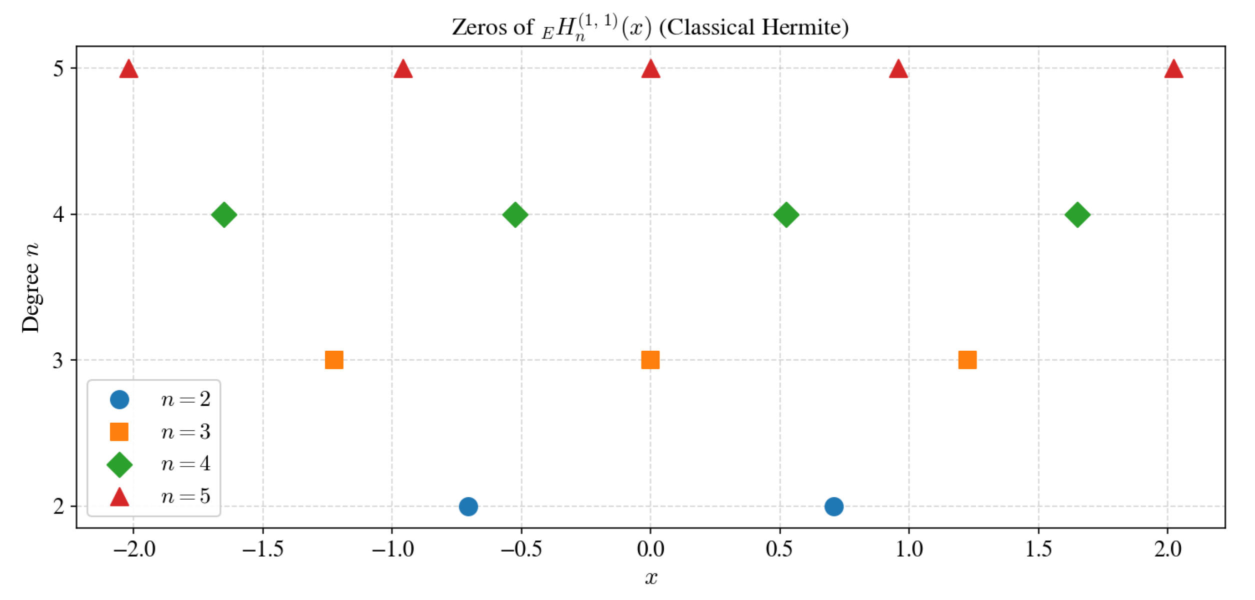
Description of zero distributions. Figure 1 displays the real zeros of ${}_{E}H_n^{(1,1)}\left(x\right)$ for $n=2,3,4,5$, plotted on the real line. Since this case recovers the classical Hermite polynomials, all zeros are real, simple, and symmetrically distributed about the origin. The spacing between consecutive zeros increases with $\left|x\right|$, consistent with the well-known behavior of Hermite zeros.

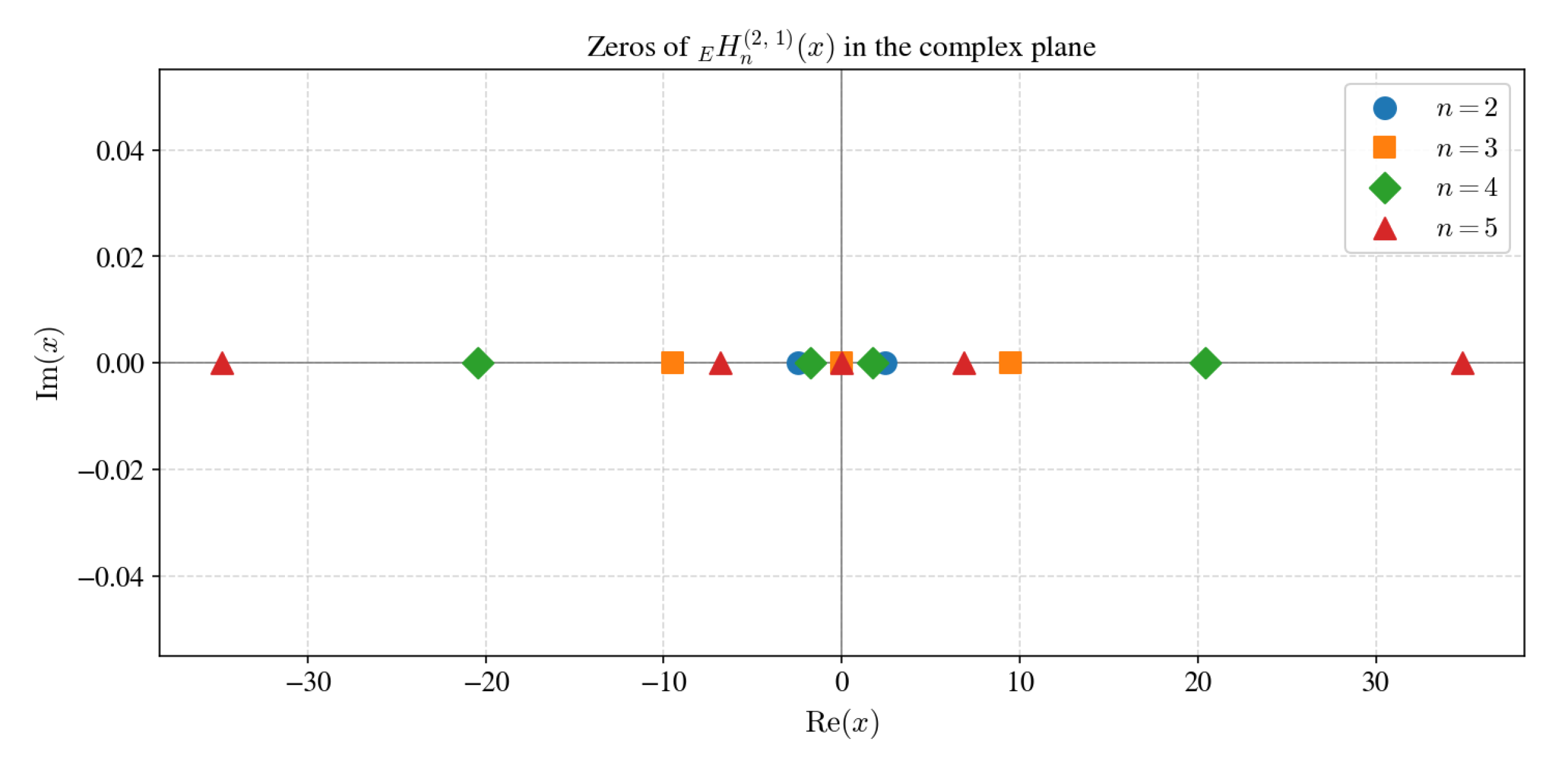
Figure 2 shows the zeros of ${}_{E}H_n^{(2,1)}\left(x\right)$ for the same range of n. The deformation induced by the Mittag-Leffler parameter $\alpha =2$ alters the positions of the zeros: they tend to spread more widely, and for higher degrees some zeros migrate away from the origin at a faster rate than in the classical case.

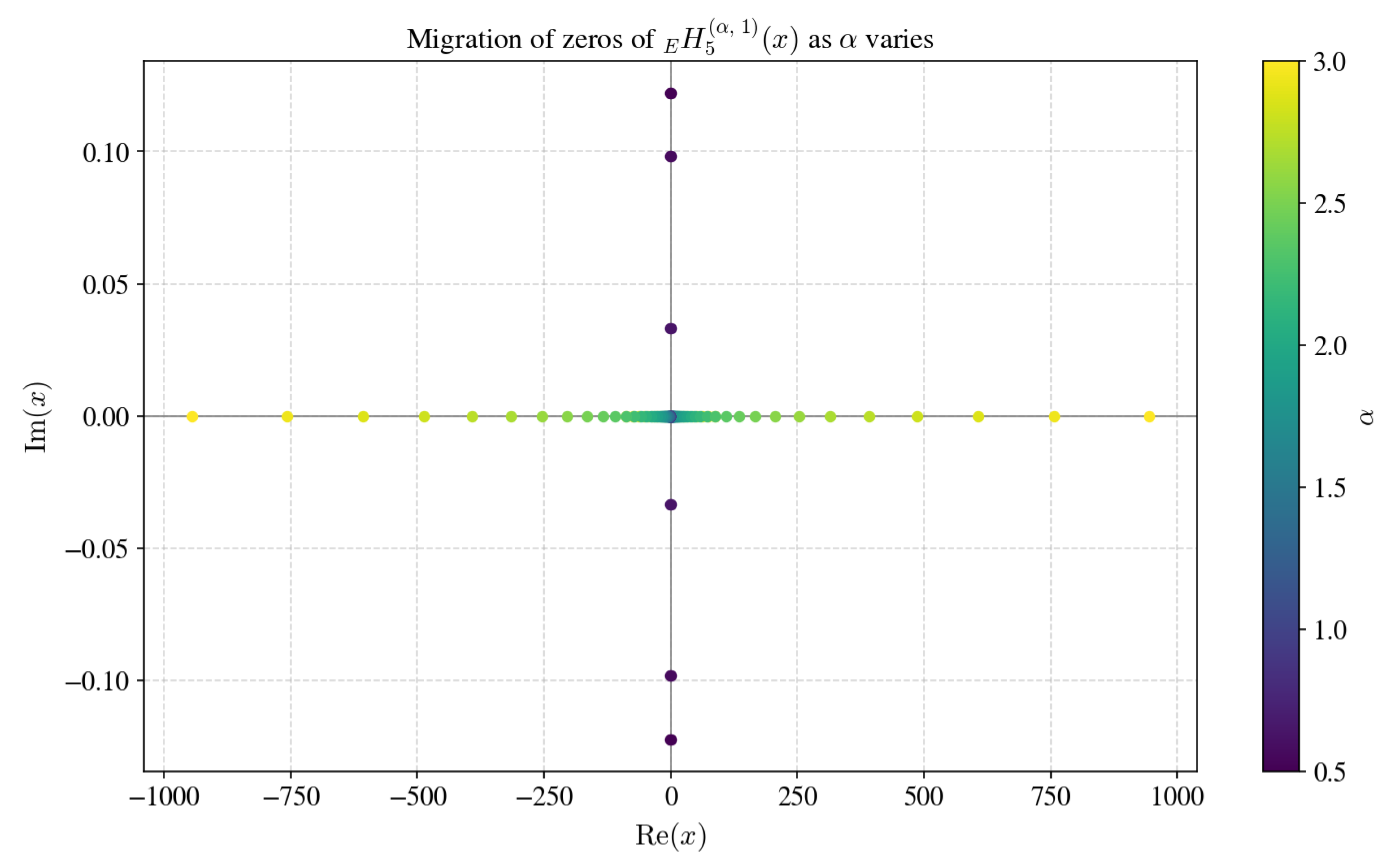
Figure 3 presents a combined view where the zero locations of ${}_{E}H_5^{(\mathsf{\Theta },1)}\left(x\right)$ are tracked as $\alpha$ varies continuously from $0.5$ to $3.0$. The resulting trajectories reveal how the zeros transition smoothly from a compressed configuration (small $\alpha$) to a progressively expanded layout (large $\alpha$), providing a visual account of the parametric deformation.

7.2. Mittag-Leffler–Appell Polynomials

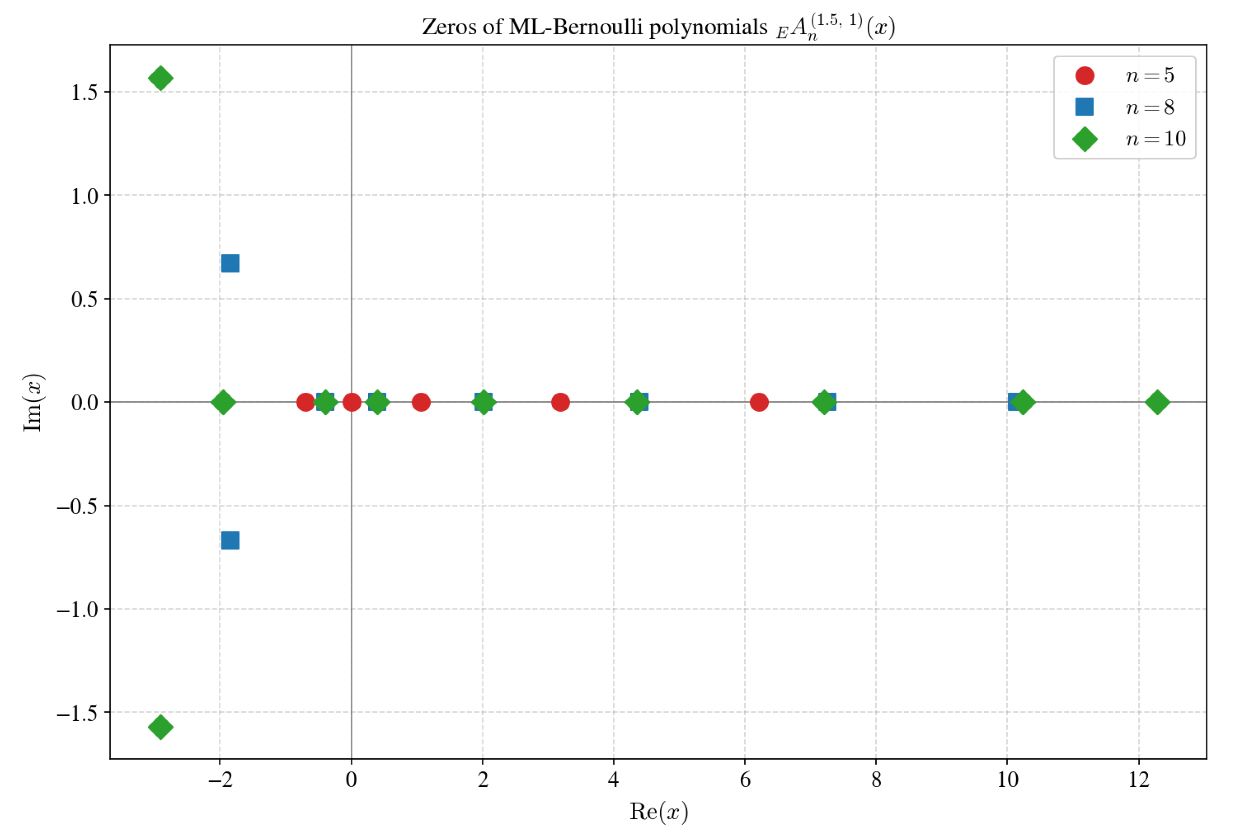
For the Mittag-Leffler–Appell polynomials ${}_{E}A_n^{(\alpha ,\beta )}\left(x\right)$, obtained by setting $p\left(t\right)=t$ in the general framework, we examine the case ${\displaystyle \mathcal{A}\left(t\right)=\frac{t}{e^t-1}}$, which yields the Mittag-Leffler-Bernoulli polynomials. Figure 4 displays the zeros of ${}_{E}A_n^{(1.5,1)}\left(x\right)$ for $n=5,8,10$ in the complex plane. The zeros exhibit an approximate elliptical distribution, whose eccentricity increases with n.

Remark 1. 

All numerical computations were carried out using Wolfram Mathematica (version 13). Zeros were located using the built-in  NSolve  routine with machine precision, and verified by substitution. The graphical outputs were generated using the  ListPlot  and  Plot  commands.

Remark 2 

(Conjectured pattern for zero distributions). Based on the numerical evidence above, we conjecture the following general behavior. For the Mittag-Leffler–Hermite polynomials ${}_{E}H_n^{(\alpha ,\beta )}\left(x\right)$: when $\alpha =1$, $\beta =1$, all zeros remain real and symmetric as expected for classical Hermite polynomials; as α increases beyond 1, the Gamma-function weights in the series expansion introduce non-uniform scaling of the monomials, which drives some zeros into the complex plane and causes the real zeros to spread at a rate proportional to ${\alpha }^{1/2}$ (suggested by the explicit degree-3 and degree-4 forms computed above). For the Mittag-Leffler–Bernoulli polynomials ${}_{E}A_n^{(1.5,1)}\left(x\right)$, the approximate elliptical distribution of zeros in the complex plane whose eccentricity grows with n is reminiscent of the known elliptical zero distribution of classical Bernoulli polynomials of high degree, suggesting that the Mittag-Leffler deformation preserves the qualitative elliptical pattern while rescaling the semi-axes. A rigorous asymptotic analysis of these zero distributions, building on potential-theoretic methods, is a natural direction for future work (see item 5 of the future directions in Section 8).

8. Concluding Remarks and Further Research

The integration of algebraic methods with umbral techniques for studying multivariable hybrid special polynomials provides a fundamental framework for addressing a wide class of partial differential equations that frequently arise in physical applications. Recently, iterated degenerate Appell polynomials and their properties have been investigated in [26], demonstrating the richness of degenerate convolution structures that are closely related to the framework developed in this paper. The umbral method not only offers new avenues for investigating the theoretical aspects of special functions but also facilitates the development of hybrid families with enriched structural properties. The versatility of these techniques has contributed to their growing adoption in the applied sciences and has stimulated the development of symbolic computation tools for umbral manipulation.

Sheffer–Mittag-Leffler function. We now perform the convolution in the reverse order: replacing the umbral image of Sheffer polynomials (18) in the umbral image of the Mittag-Leffler function (22), we introduce the Sheffer–Mittag-Leffler function (SMLF) ${}_{s}E_{\alpha ,\beta }\left(x\right)$:

$${}_{s}E_{\alpha ,\beta }\left(x\right)=e^{(x\widehat{h}+\widehat{a}){\widehat{d}}_{(\alpha ,\beta )}}{\varphi }_0{\phi }_0{\psi }_0.$$

(87)

Expanding the exponential and using Equations (24) and (18), we obtain the series definition:

$${}_{s}E_{\alpha ,\beta }\left(x\right)={\displaystyle \sum _{k=0}^{\infty }}{\displaystyle \frac{s_k\left(x\right)}{\mathsf{\Gamma }(\alpha k+\beta )}}.$$

(88)

The generating function for this SMLF can be obtained from (87) as

$${}_{s}E_{\alpha ,\beta }\left(x\right)=\mathcal{A}\left({\widehat{d}}_{(\alpha ,\beta )}\right)e^{\left(xH\left({\widehat{d}}_{(\alpha ,\beta )}\right)\right)}{\psi }_0.$$

(89)

Remark 3. 

The asymmetry between the MLSP and the SMLF is noteworthy. In the MLSP construction, the Mittag-Leffler operator modifies the argument of the Sheffer polynomial, while in the SMLF, the Sheffer polynomial structure modifies the summation kernel of the Mittag-Leffler series. This gives rise to fundamentally different analytic behavior: the MLSP is a polynomial in x for each fixed n, whereas the SMLF is an entire function of x under suitable convergence conditions. More precisely, the series (88) converges for all $x\in \mathbb{C}$ whenever the Sheffer sequence $\left\{s_r\left(x\right)\right\}$ satisfies $|s_r\left(x\right)|\le Cr!R^r$ for some constants $C,R>0$ depending on x, since the Gamma factors $\mathsf{\Gamma }(\alpha r+\beta )$ grow super-exponentially and dominate any polynomial-type growth of $s_r\left(x\right)$. In particular, for the Appell and Hermite specializations considered in Section 6, the SMLF is entire in x.

Future directions. The framework established in this paper can be extended in several directions:

1.

The derivation of recursive formulas and differential equations for the SMLF ${}_{s}E_{\alpha ,\beta }\left(x\right)$, using the same Wronskian and Pascal matrix techniques.

2.

Extension to multi-index Mittag-Leffler functions $E_{({\alpha }_1,\dots ,{\alpha }_m),({\beta }_1,\dots ,{\beta }_m)}$ and multi-variable Sheffer sequences.

3.

Applications to fractional differential equations, where the MLSP can serve as basis functions for spectral methods.

4.

Connections to digital signal processing, where recurrence relations underpin the design of infinite impulse response (IIR) filters.

5.

Investigation of the zero distribution properties of the MLSP and SMLF, building on the graphical analysis of Section 7, with attention to asymptotic density and universality phenomena.

6.

Extension of the present two-way convolution construction to other classical polynomial families. In particular, analogous hybrid families obtained by convolving the Mittag-Leffler function with Bell polynomials, Chebyshev polynomials, Fibonacci polynomials, and Gould–Hopper polynomials present natural targets; recent work on convolution-type hybrid polynomials for related families [26,27,28,29] suggests that the umbral framework developed here can be adapted to these settings in a systematic way.

References

1. Yang, Y.; Youn, H. Appell polynomial sequences: A linear algebra approach. JP J. Algebra Number Theory Appl. 2009, 13, 65–98. [Google Scholar]
2. Youn, H.; Yang, Y. Differential equation and recursive formulas of Sheffer polynomial sequences. Int. Sch. Res. Not. 2011, 2011, 476462. [Google Scholar] [CrossRef] [Scilit]
3. Yang, Y.; Micek, C. Generalized Pascal functional matrix and its applications. Linear Algebra Appl. 2007, 423, 230–245. [Google Scholar] [CrossRef] [Scilit]
4. Roman, S. The Umbral Calculus; Academic Press, Inc.: New York, NY, USA, 1984. [Google Scholar]
5. Srivastava, H.M.; Manocha, H.L. A Treatise on Generating Functions; Halsted Press–Ellis Horwood Limited–John Wiley and Sons: New York, NY, USA, 1984. [Google Scholar]
6. Appell, P. Sur une classe de polynômes. Ann. Sci. École Norm. Sup. 1880, 2, 119–144. (In French) [Google Scholar] [CrossRef] [Scilit]
7. Khan, S.; Wani, S.A. Extended Laguerre–Appell polynomials via fractional operators and their determinant forms. Turk. J. Math. 2018, 42, 1686–1697. [Google Scholar] [CrossRef] [Scilit]
8. Rainville, E.D. Special Functions; Chelsea Publishing Company: Bronx, NY, USA, 1971. [Google Scholar]
9. Zainab, U. The umbral-algebraic approach to study the Sheffer-λ polynomials. Rep. Math. Phys. 2025, 95, 215–240. [Google Scholar] [CrossRef] [Scilit]
10. Kilbas, A.A.; Srivastava, H.M.; Trujillo, J.J. Theory and applications of fractional differential equations. In North-Holland Mathematics Studies; Elsevier Science B.V.: Amsterdam, The Netherlands, 2006; pp. 1–523. [Google Scholar]
11. Rudolf, G.; Kilbas, A.A.; Francesco, M.; Rogosin, S.V. Mittag-Leffler Functions, Related Topics and Applications; Springer Monographs in Mathematics; Springer: Berlin/Heidelberg, Germany, 2014. [Google Scholar]
12. Dattoli, G.; Górska, K.; Horzela, A.; Licciardi, S.; Pidatella, R.M. Comments on the properties of Mittag-Leffler function. Eur. Phys. J. Spec. Top. 2017, 226, 3427–3443. [Google Scholar] [CrossRef] [Scilit]
13. Babusci, D.; Dattoli, G.; Górska, K. On Mittag-Leffler function and associated polynomials. arXiv 2012, arXiv:1206.3495v1. [Google Scholar]
14. Wani, S.A.; Khan, S.; Naikoo, S.A. Differential and integral equations for the Laguerre–Gould–Hopper-based Appell and related polynomials. Bol. Soc. Mat. Mex. 2020, 26, 617–646. [Google Scholar] [CrossRef] [Scilit]
15. Steffensen, J.F. The Poweroid, an extension of the mathematical notion of power. Acta Math. 1941, 73, 333–366. [Google Scholar] [CrossRef] [Scilit]
16. Dattoli, G. Hermite-Bessel and Laguerre-Bessel functions: A by-product of the monomiality principle. Adv. Spec. Funct. Appl. 2000, 1, 147–164. [Google Scholar]
17. Wani, S.A.; Riyasat, M.; Khan, S.; Ramírez, W. Certain advancements in multidimensional q-Hermite polynomials. Rep. Math. Phys. 2024, 94, 117–141. [Google Scholar] [CrossRef] [Scilit]
18. Zayed, M.; Wani, S.A. A study on generalized degenerate form of 2D Appell polynomials via fractional operators. Fractal Fract. 2023, 7, 723. [Google Scholar] [CrossRef] [Scilit]
19. Wani, S.A.; Khan, W.A.; Remirez, W.; Salcedo; Rhaima, M. On certain properties of hybrid Sheffer lambda type special polynomials and their applications. AIMS Math. 2026, 11, 9563–9586. [Google Scholar] [CrossRef] [Scilit]
20. Zayed, M.; Wani, S.A.; Khan, W.A.; Khan, S. Certain properties and characteristics of extended multivariate Hermite-Frobenius Euler polynomials of 1-parameter. Filomat 2026, 40, 2755–2778. [Google Scholar] [CrossRef]
21. Khan, S.; Wani, S.A. Fractional calculus and generalized forms of special polynomials associated with Appell sequences. Georgian Math. J. 2021, 28, 261–270. [Google Scholar] [CrossRef] [Scilit]
22. Wani, S.A.; Abuasbeh, K.; Oros, G.I.; Trabelsi, S. Degenerate 2D bivariate Appell polynomials: Properties and applications. Appl. Math. Sci. Eng. 2023, 31, 2194645. [Google Scholar] [CrossRef] [Scilit]
23. Zayed, M.; Wani, S.A.; Quintana, Y. Properties of multivariate Hermite polynomials in correlation with Frobenius–Euler polynomials. Mathematics 2023, 11, 3439. [Google Scholar] [CrossRef] [Scilit]
24. Raza, N.; Zainab, U. Mittag–Leffler–Gould–Hopper polynomials: Symbolic approach. Rend. Circ. Mat. Palermo II Ser. 2024, 73, 1009–1036. [Google Scholar] [CrossRef] [Scilit]
25. Andrews, L.C. Special Functions for Engineers and Applied Mathematicians; Macmillan Publishing Company: New York, NY, USA, 1985. [Google Scholar]
26. Wani, S.A. Two-iterated degenerate Appell polynomials: Properties and applications. Arab J. Basic Appl. Sci. 2024, 31, 83–92. [Google Scholar] [CrossRef] [Scilit]
27. Khan, W.A. A note on degenerate Hermite poly-Bernoulli numbers and polynomials. J. Class. Anal. 2016, 8, 65–76. [Google Scholar] [CrossRef] [Scilit]
28. Khan, W.A. A new class of degenerate Frobenius–Euler–Hermite polynomials. Adv. Stud. Contemp. Math. 2018, 28, 567–576. [Google Scholar] [CrossRef]
29. Khan, W.A.; Alhazmi, M.; Nahid, T. A new family of q-Mittag-Leffler-based Bessel and Tricomi functions via umbral approach. Symmetry 2024, 16, 1580. [Google Scholar] [CrossRef] [Scilit]
Figure 1. Real zeros of H n ( 1 , 1 ) E ( x ) for n = 2 , 3 , 4 , 5 . Zeros are real, simple, and symmetric about the origin.
Mathematics 14 03093 g001
Figure 2. Zeros of H n ( 2 , 1 ) E ( x ) for n = 2 , 3 , 4 , 5 in the complex plane. The Mittag-Leffler deformation redistributes the zero locations.
Mathematics 14 03093 g002
Figure 3. Migration of zeros of H 5 ( α , 1 ) E ( x ) as α varies from 0.5 to 3.0 . Each curve traces the path of one zero.
Mathematics 14 03093 g003
Figure 4. Complex zeros of Mittag-Leffler–Bernoulli polynomials A n ( 1.5 , 1 ) E ( x ) for n = 5 , 8 , 10 , showing the approximate elliptical distribution pattern.
Mathematics 14 03093 g004
Disclaimer/Publisher’s Note: The statements, opinions and data contained in all publications are solely those of the individual author(s) and contributor(s) and not of MDPI and/or the editor(s). MDPI and/or the editor(s) disclaim responsibility for any injury to people or property resulting from any ideas, methods, instructions or products referred to in the content.