A General Framework for Stability Analysis of Neutral Cohen–Grossberg Neural Networks with Discrete Delay Terms

Abstract

This paper studies global asymptotic stability of Cohen–Grossberg neural networks involving discrete time delays in the neuron states and neutral delays in the time derivatives of the neuron states. An appropriate Lyapunov functional, which is defined by the linear combination of three Lyapunov functionals of the quadratic forms, is constructed to determine new criteria for global asymptotic stability of neutral-type neural networks with discrete delay parameters. The proposed stability conditions are established through a set of algebraic inequalities that utilize key matrix properties and parameters of system functions. These criteria are proved to be independent of delay components, and they can be tested by checking some algebraic inequalities. A numerical example is studied to illustrate the efficiency aspects of the derived stability conditions.

1. Introduction

The class of dynamical neural networks has recently attracted considerable attention, since these networks have proved to possess extensive applications in real-world engineering problems with regard to global pattern formation [1], emergent collective computational abilities [2,3], nonlinear programming [4], fixed point learning algorithms [5], optimization problems [6], signal processing [7], and analog neural nonlinear programming solvers [8]. In most of these applications, the information representing the studied problem is generally required to be properly processed in the form of stable states of the network neurons. In this context, it is of crucial importance to determine the stability properties of the equilibrium points associated with neural networks. In the past literature, the stability issue of dynamical neural networks has gained a great deal of attention, and some key results addressing the stability of neural networks have been proposed (see [9,10,11,12] and references therein). It is known from the literature that, in the electronic implementation of a dynamical neural network by electronic circuit components, time delay elements are unavoidably present as a consequence of the finite switching speeds of the network amplifiers as well as the inherent communication times of the network neurons. Thus, the existence of time delay components usually has critical impacts on the stability of neural networks, leading to undesired oscillatory and unstable behaviors [13,14,15]. Therefore, the time delays involved in the dynamics of the neurons describe the dynamical behaviors of the neuron model more precisely. In the process of determining the desired stability criteria for neural networks, the selection of suitable Lyapunov functionals plays a crucial role. Recently, various forms of suitable Lyapunov functionals have been constructed to derive alternative sets of stability criteria associated with different models of delayed dynamical neural networks. In [16,17,18,19], robust stability of neural networks involving multiple discrete delays has been studied; in [20,21,22,23], stability of neural networks with discrete and distributed delays has been investigated; and in [24], stability of delayed fuzzy inertial discontinuous neural networks has been analyzed. In these papers, various sets of stability criteria for the considered neural network models have been derived by constructing suitable Lyapunov functionals, and using some matrix and norm inequalities. We now note that dynamical neural networks can also be modelled by neutral functional differential equations, which include both time and neutral delay arguments. This class of neural systems is generally called neutral-type neural networks. In this neural network model, both states and time derivatives of states contain delay parameters. The dynamical systems defined by neutral-type differential equations are usually employed in the mathematical modelling of engineering problems including the dynamical modelling of the unsteady motion of the elastic rigid body [25]; the optimal control and automatic control problems [26]; viscoelasticity [27]; the lossless transmission lines [28]; cell growth [29]; the economic models [30]; and the population models [31]. Therefore, substantial research has been conducted to establish stability conditions for neutral neural networks. Recently, numerous articles have employed various Lyapunov functional candidates to determine stability conditions for different classes of neutral Hopfield neural networks. In [32], stability problem for the class of neutral high-order Hopfield neural networks with mixed time delays has been studied. In [33,34,35,36], stability conditions for the class of Hopfield neural networks with multiple delays have been presented. In [37,38,39,40], stability of the class of neutral Hopfield neural networks with a single time delay and a single neutral delay has been investigated. In [41,42,43], stability of neutral Hopfield neural networks with time-varying delays has been studied.

This current article will deal with the stability problem for neutral Cohen–Grossberg neural networks, which is a more general class of neural networks than Hopfield neural networks. A novel Lyapunov functional method, combining a set of the Lyapunov functionals, together with using matrix analysis techniques, is constructed to obtain the criteria under which the examined neutral neural system is globally asymptotically stable. Our proposed stability criteria mainly involve network parameters, that can merely be checked by verifying some system-related algebraic equations. In addition, stability conditions given in this paper are purely delay-independent; that is, they are independent of the size of delay terms. It is indicated that most of the previous stability results presented for various versions of the same neural network model can be obtained from the appropriate choices of set of the Lyapunov functionals utilized in this paper.

Notations: Throughout this paper, $x\in {\mathbb{R}}^n$ denotes a real vector $x={(x_1,x_2,\dots ,x_n)}^T$ and $A\in {\mathbb{R}}^{n\times n}$ denotes a real matrix $A={\left(a_{ij}\right)}_{n\times n}$. $x^T$ represents the transpose of vector x. $A^T$ and $A^{-1}$ respectively denote the transpose and inverse of A. I denotes the identity matrix of the appropriate dimension. $D=\mathrm{diag}(d_i>0)$ is a positive diagonal matrix with the entries $d_i>0,i=1,\dots ,n$. For the elements $d_1,d_2,\dots ,d_n$, $d_m$ and $d_M$ will respectively denote $d_m={min}_{1\le i\le n}\left\{d_i\right\}$ and $d_M={max}_{1\le i\le n}\left\{d_i\right\}$. Finally, the vector and matrix norms are noted: ${||x||}_2=\sqrt{{\sum }_{i=1}^n{x}_i^2}{\mathrm{and}||A||}_2=\sqrt{{\lambda }_M\left(A^{T}A\right)}$ where ${\lambda }_M\left(A^{T}A\right)$ is the maximum eigenvalue of the nonnegative definite matrix $A^{T}A$.

2. Neutral Cohen–Grossberg Neural Networks

This study will deal with stability problem for the neutral Cohen–Grossberg neural network that is defined by the nonlinear differential equations given by

$$\begin{array}{cc}\hfill {\dot{x}}_i\left(t\right)=& d_i\left(x_i\left(t\right)\right)(-c_i\left(x_i\left(t\right)\right)+{\displaystyle \sum _{j=1}^n}{a}_{ij}{f}_j\left(x_j\left(t\right)\right)+{\displaystyle \sum _{j=1}^n}{b}_{ij}{f}_j\left(x_j(t-{\tau }_j)\right)+u_i)\hfill \\ \hfill & +{\displaystyle \sum _{j=1}^n}{e}_{ij}{\dot{x}}_j(t-{\zeta }_j),i=1,\dots ,n.\hfill \end{array}$$

(1)

where

• n indicates the number of neurons involved in system (1);
• $x_i\left(t\right)$ is the state of ith neuron;
• $a_{ij}$ and $b_{ij}$ are the constant interconnection elements;
• $e_{ij}$ are the constant coefficients of time derivatives of states with neutral delays;
• $d_i\left(x_i\left(t\right)\right)$ are the amplification functions;
• $c_i\left(x_i\left(t\right)\right)$ are the behaved functions;
• $f_i\left(x_i\left(t\right)\right)$ are the nonlinear activation functions;
• ${\tau }_i$ are the constant time delays;
• ${\zeta }_i$ are the constant neutral delays;
• $u_i$ are the constant inputs, $i,j=1,\dots ,n$.

In neutral system (1), let ${\tau }_M={max}_{1\le i\le n}\left\{{\tau }_i\right\}$, ${\zeta }_M={max}_{1\le i\le n}\left\{{\zeta }_i\right\}$ and $\chi =max\{{\tau }_M,{\zeta }_M\}$. Then, the accompanying initial data of the neutral-type neural network (1) are introduced by

$$x_i\left(t\right)={\phi }_i\left(t\right)\in C([-\chi ,0],\mathbb{R}),\dot{x_i}\left(t\right)={\widehat{\phi }}_i\left(t\right)={\displaystyle \frac{d}{dt}}{\phi }_i\left(t\right)\in C([-\chi ,0],\mathbb{R})$$

where $C\left(\right[-\chi ,0],\mathbb{R})$ denotes the set of all continuous functions from $[-\chi ,0]$ to $\mathbb{R}$.

When dealing with stability issues for the neutral system described by (1), we first need to know the mathematical statements of the amplification functions $d_i\left(x_i\left(t\right)\right)$, the behaved functions $c_i\left(x_i\left(t\right)\right)$ and the activation functions $f_i\left(x_i\left(t\right)\right)$ included in neural system (1). In general, the system functions are considered to satisfy the properties given below:

${\mathcal{A}}_1$: The amplification functions $d_i\left(x\right)$ are considered to satisfy the conditions:

$$\begin{array}{c}\hfill 0<{\upsilon }_i\le d_i\left(x\right)\le {\varphi }_i,\forall x\in \mathbb{R},\forall i\end{array}$$

with ${\upsilon }_i$ and ${\varphi }_i$ being positive real constants.

${\mathcal{A}}_2$: The behaved functions $c_i\left(x\right)$ are considered to satisfy the conditions:

$$\begin{array}{c}\hfill {\alpha }_i\le {\displaystyle \frac{c_i\left(x\right)-c_i\left(z\right)}{x-z}}\le {\ell }_i,\forall x,z\in \mathbb{R},x\ne z,\forall i\end{array}$$

with ${\alpha }_i$ and ${\ell }_i$ being positive real constants.

${\mathcal{A}}_3$: The nonlinear activation functions $f_i\left(x\right)$ are considered to possess the Lipschitz property given by

$$\begin{array}{c}\hfill |f_i\left(x\right)-f_i\left(z\right)|\le l_i|x-z|,\forall x,z\in \mathbb{R},\forall i\end{array}$$

where $l_i$ are positive constants.

3. Stability Analysis

In this section, by utilizing various linear combinations of different types of Lyapunov functional candidates, which are stated in terms of the squares of the states of the neurons, many novel sets of sufficient criteria associated with the global asymptotic stability of the neural network described in (1) will be derived. Assume that neural system (1) has an equilibrium point for a particular input $u={(u_1,u_2,\dots ,u_n)}^T$ and denote this equilibrium point by $x^{\ast }={(x_1^{\ast },x_2^{\ast },\dots ,x_n^{\ast })}^T$. Now, transform (1) into an equivalent neural network model by using $s_i\left(t\right)=x_i\left(t\right)-x_i^{\ast },\forall i$. With the help of this transformation, neural network (1) is directly stated in the transformed form given by

$$\begin{array}{cc}\hfill {\dot{s}}_i\left(t\right)=& {\gamma }_i\left(s_i\left(t\right)\right)(-{\rho }_i\left(s_i\left(t\right)\right)+{\displaystyle \sum _{j=1}^n}{a}_{ij}{g}_j\left(s_j\left(t\right)\right)+{\displaystyle \sum _{j=1}^n}{b}_{ij}{g}_j\left(s_j(t-{\tau }_j)\right))\hfill \\ \hfill & +{\displaystyle \sum _{j=1}^n}{e}_{ij}{\dot{s}}_j(t-{\zeta }_j),\forall i\hfill \end{array}$$

(2)

where the new nonlinear functions in the transformed system possess the forms: ${\gamma }_i\left(s_i\left(t\right)\right)=d_i(s_i\left(t\right)+x_i^{\ast })$, ${\rho }_i\left(s_i\left(t\right)\right)=c_i(s_i\left(t\right)+x_i^{\ast })-c_i\left(x_i^{\ast }\right)$ and $g_i\left(s_i\left(t\right)\right)=f_i(s_i\left(t\right)+x_i^{\ast })-f_i\left(x_i^{\ast }\right)$. Based on ${\mathcal{A}}_1-{\mathcal{A}}_3$, these functions satisfy the conditions:

$$\begin{gathered} {\mathcal{C}}_1:{\upsilon }_i\le {\gamma }_i\left(s_i\left(t\right)\right)\le {\varphi }_i,\forall i, \\ \hspace{1em}\hspace{1em}\hspace{1em}\hspace{1em}\hspace{1em} {\mathcal{C}}_2:{\alpha }_i{s}_i^2\left(t\right)\le s_i\left(t\right){\rho }_i\left(s_i\left(t\right)\right)\le {\ell }_i{s}_i^2\left(t\right),\forall i, \\ \hspace{1em} {\mathcal{C}}_3:\mid g_i\left(s_i\left(t\right)\right)\mid \le l_i\mid \left(s_i\left(t\right)\right)\mid ,\forall i. \end{gathered}$$

The vector-matrix representation of neural network (2) is written as

$$\dot{s}\left(t\right)=\mathrm{\Gamma }\left(s\left(t\right)\right)(-\rho \left(s\left(t\right)\right)+Ag\left(s\left(t\right)\right)+Bg\left(s(t,\tau )\right))+E\dot{s}(t,\zeta )$$

(3)

where

• $s\left(t\right)={(s_1\left(t\right),s_2\left(t\right),\dots ,s_n\left(t\right))}^T$ is the state vector of the system;
• A, B and E are the constant system matrices;
• $\mathrm{\Gamma }\left(s\left(t\right)\right)=\mathrm{diag}({\gamma }_i\left(s_i\left(t\right)\right)>0)$ is a positive diagonal matrix;
• $\rho \left(s\left(t\right)\right)={({\rho }_1\left(s_1\left(t\right)\right),{\rho }_2\left(s_2\left(t\right)\right),\dots ,{\rho }_n\left(s_n\left(t\right)\right))}^T$;
• $g\left(s\left(t\right)\right)={(g_1\left(s_1\left(t\right)\right),g_2\left(s_2\left(t\right)\right),\dots ,g_n\left(s_n\left(t\right)\right))}^T$ is the output vector;
• $g\left(s(t,\tau )\right)={(g_1\left(s_1(t-{\tau }_1)\right),g_2\left(s_2(t-{\tau }_2)\right),\dots ,g_n\left(s_n(t-{\tau }_n)\right))}^T$;
• $\dot{s}(t,\zeta )={({\dot{s}}_1(t-{\zeta }_1),{\dot{s}}_2(t-{\zeta }_2),\dots ,{\dot{s}}_n(t-{\zeta }_n))}^T$.

Note that neural systems (1) and (2) have equivalent stability properties. Therefore, we will simply conduct the stability analysis for the origin of neural system (2) without conducting the stability analysis for the equilibrium points associated with neural system (1). Before proceeding any further, in order to establish a general framework for the stability conditions of neutral system (2), it is necessary to give the following key lemma of the paper:

Lemma 1.

For ${\gamma }_i\left(s_i\left(t\right)\right)$ in system (2), define

$${\psi }_i\left(s_i\left(t\right)\right)=k_1+k_2{\gamma }_i\left(s_i\left(t\right)\right)+{\displaystyle \frac{k_3}{{\gamma }_i\left(s_i\left(t\right)\right)}},{\widehat{\psi }}_i\left(s_i\left(t\right)\right)={\widehat{k}}_1+{\widehat{k}}_2{\gamma }_i\left(s_i\left(t\right)\right)+{\displaystyle \frac{{\widehat{k}}_3}{{\gamma }_i\left(s_i\left(t\right)\right)}}$$

and

$${\tilde{\psi }}_i\left(s_i\left(t\right)\right)={\displaystyle \frac{{\tilde{k}}_1}{{\gamma }_i\left(s_i\left(t\right)\right)}}+{\tilde{k}}_2+{\displaystyle \frac{{\tilde{k}}_3}{{\gamma }_i^2\left(s_i\left(t\right)\right)}},\forall i$$

where $k_1$, $k_2$, $k_3$, ${\widehat{k}}_1$, ${\widehat{k}}_2$, ${\widehat{k}}_3$, ${\tilde{k}}_1$, ${\tilde{k}}_2$ and ${\tilde{k}}_3$ are the nonnegative real constants with $k_1+k_2+k_3={\widehat{k}}_1+{\widehat{k}}_2+{\widehat{k}}_3={\tilde{k}}_1+{\tilde{k}}_2+{\tilde{k}}_3=1$. Then, the following conditions hold

$$\begin{array}{cc}\hfill & {\mathrm{{\rm Y}}}_i=k_1{\upsilon }_i+k_2{\upsilon }_i^2+k_3\le {\gamma }_i\left(s_i\left(t\right)\right){\psi }_i\left(s_i\left(t\right)\right)=k_1{\gamma }_i\left(s_i\left(t\right)\right)+k_2{\gamma }_i^2\left(s_i\left(t\right)\right)+k_3\hfill \\ \hfill & \phantom{{\mathrm{{\rm Y}}}_i}\le k_1{\varphi }_i+k_2{\varphi }_i^2+k_3={\mathrm{\Omega }}_i,\hfill \\ \hfill & {\mathrm{\Theta }}_i={\displaystyle \frac{k_1}{{\varphi }_i}}+k_2+{\displaystyle \frac{k_3}{{\varphi }_i^2}}\le {\displaystyle \frac{{\psi }_i\left(s_i\left(t\right)\right)}{{\gamma }_i\left(s_i\left(t\right)\right)}}={\displaystyle \frac{k_1}{{\gamma }_i\left(s_i\left(t\right)\right)}}+k_2+{\displaystyle \frac{k_3}{{\gamma }_i^2\left(s_i\left(t\right)\right)}}\le {\displaystyle \frac{k_1}{{\upsilon }_i}}+k_2+{\displaystyle \frac{k_3}{{\upsilon }_i^2}}={\mathrm{\Phi }}_i\hfill \\ \hfill & {\widehat{\psi }}_i\left(s_i\left(t\right)\right)={\widehat{k}}_1+{\widehat{k}}_2{\gamma }_i\left(s_i\left(t\right)\right)+{\displaystyle \frac{{\widehat{k}}_3}{{\gamma }_i\left(s_i\left(t\right)\right)}}\le {\widehat{k}}_1+{\widehat{k}}_2{\varphi }_i+{\displaystyle \frac{{\widehat{k}}_3}{{\upsilon }_i}}={\widehat{\mathrm{\Lambda }}}_i\hfill \\ \hfill & {\widehat{\mathrm{\Theta }}}_i={\displaystyle \frac{{\widehat{k}}_1}{{\varphi }_i}}+{\widehat{k}}_2+{\displaystyle \frac{{\widehat{k}}_3}{{\varphi }_i^2}}\le {\displaystyle \frac{{\widehat{\psi }}_i\left(s_i\left(t\right)\right)}{{\gamma }_i\left(s_i\left(t\right)\right)}}={\displaystyle \frac{{\widehat{k}}_1}{{\gamma }_i\left(s_i\left(t\right)\right)}}+{\widehat{k}}_2+{\displaystyle \frac{{\widehat{k}}_3}{{\gamma }_i^2\left(s_i\left(t\right)\right)}}\le {\displaystyle \frac{{\widehat{k}}_1}{{\upsilon }_i}}+{\widehat{k}}_2+{\displaystyle \frac{{\widehat{k}}_3}{{\upsilon }_i^2}}={\widehat{\mathrm{\Phi }}}_i\hfill \end{array}$$

$$\begin{array}{cc}\hfill & {\widetilde{\mathrm{{\rm Y}}}}_i={\tilde{k}}_1+{\tilde{k}}_2{\upsilon }_i+{\displaystyle \frac{{\tilde{k}}_3}{{\varphi }_i}}\le {\gamma }_i\left(s_i\left(t\right)\right){\tilde{\psi }}_i\left(s_i\left(t\right)\right)={\tilde{k}}_1+{\tilde{k}}_2{\gamma }_i\left(s_i\left(t\right)\right)+{\displaystyle \frac{{\tilde{k}}_3}{{\gamma }_i\left(s_i\left(t\right)\right)}}\hfill \\ \hfill & \phantom{{\widetilde{\mathrm{{\rm Y}}}}_i}\le {\tilde{k}}_1+{\tilde{k}}_2{\varphi }_i+{\displaystyle \frac{{\tilde{k}}_3}{{\upsilon }_i}}={\tilde{\mathrm{\Lambda }}}_i\hfill \\ \hfill & {\tilde{\psi }}_i\left(s_i\left(t\right)\right)={\displaystyle \frac{{\tilde{k}}_1}{{\gamma }_i\left(s_i\left(t\right)\right)}}+{\tilde{k}}_2+{\displaystyle \frac{{\tilde{k}}_3}{{\gamma }_i^2\left(s_i\left(t\right)\right)}}\le {\displaystyle \frac{{\tilde{k}}_1}{{\upsilon }_i}}+{\tilde{k}}_2+{\displaystyle \frac{{\tilde{k}}_3}{{\upsilon }_i^2}}={\tilde{\mathrm{\Phi }}}_i,\forall i\hfill \\ \hfill & {\parallel \mathrm{\Gamma }\left(s\left(t\right)\right)\mathrm{\Psi }\left(s\left(t\right)\right)\parallel }_2\le k_1{\varphi }_M+k_2{\varphi }_M^2+k_3={\mathrm{\Omega }}_M\hfill \\ \hfill & \parallel {\mathrm{\Gamma }}^{-1}{\left(s\left(t\right)\right)\mathrm{\Psi }\left(s\left(t\right)\right)\parallel }_2\le {\displaystyle \frac{k_1}{{\upsilon }_m}}+k_2+{\displaystyle \frac{k_3}{{\upsilon }_m^2}}={\mathrm{\Phi }}_M\hfill \end{array}$$

where $\mathrm{\Psi }\left(s\left(t\right)\right)=\mathrm{diag}({\psi }_i\left(s_i\left(t\right)\right)>0)=k_{1}I+k_2\mathrm{\Gamma }\left(s\left(t\right)\right)+k_3{\mathrm{\Gamma }}^{-1}\left(s\left(t\right)\right)$, ${\upsilon }_m={min}_{1\le i\le n}\left\{{\upsilon }_i\right\}$, ${\varphi }_M={max}_{1\le i\le n}\left\{{\varphi }_i\right\}$, ${\mathrm{\Phi }}_M={max}_{1\le i\le n}\left\{{\mathrm{\Phi }}_i\right\}$ and ${\mathrm{\Omega }}_M={max}_{1\le i\le n}\left\{{\mathrm{\Omega }}_i\right\}$.

Proof of Lemma 1.

The proof of this lemma directly follows from the fact that all inequalities stated in Lemma 1 hold under the condition that ${\upsilon }_i\le {\gamma }_i\left(s_i\left(t\right)\right)\le {\varphi }_i,\forall i$, defined by assumption ${\mathcal{C}}_1$. □

Exploiting the results of Lemma 1, we determine the main stability conditions as follows:

Theorem 1.

Let system (3) satisfy the conditions ${\mathcal{C}}_1-{\mathcal{C}}_3$. Then, the origin of neutral system (3) is globally asymptotically stable if the following two sets of criteria are satisfied:

$$\begin{array}{cc}\hfill {\varrho }_i=& h_1({ϵ}_i-{\delta }_i-{\xi }_i)-h_2({\widehat{\delta }}_i+{\widehat{\xi }}_i)+h_3({\widetilde{ϵ}}_i-{\tilde{\delta }}_i-{\tilde{\xi }}_i)>0\hfill \end{array}$$

and

$$\begin{array}{cc}\hfill {\vartheta }_i=& h_1({\epsilon }_i-{\sigma }_i)+h_2({\widehat{\epsilon }}_i-{\widehat{\sigma }}_i-{\widehat{\omega }}_i)-h_3{\tilde{\sigma }}_i>0,\forall i\hfill \end{array}$$

where $h_1$, $h_2$ and $h_3$ are the nonnegative constants with $h_1+h_2+h_3=1$, and

$$\begin{array}{cc}\hfill & {ϵ}_i={\mathrm{{\rm Y}}}_i{\alpha }_i^2,{\epsilon }_i={\mathrm{\Theta }}_i,{\widehat{\epsilon }}_i=2p_i{\widehat{\mathrm{\Theta }}}_i,{\widetilde{ϵ}}_i=2q_i{\widetilde{\mathrm{{\rm Y}}}}_i{\alpha }_i,\hfill \end{array}$$

$$\begin{array}{cc}\hfill {\delta }_i=& (1+\kappa +\beta )\left({\theta }_1{\mathrm{\Omega }}_M{\parallel A\parallel }_2^2+{\theta }_2{\displaystyle \sum _{j=1}^n}{\displaystyle \sum _{k=1}^n}{\mathrm{\Omega }}_k|a_{ki}||a_{kj}|\right)l_i^2,\hfill \\ \hfill {\xi }_i=& (1+{\displaystyle \frac{1}{\kappa }}+\eta )\left({\mu }_1{\mathrm{\Omega }}_M{\parallel B\parallel }_2^2+{\mu }_2{\displaystyle \sum _{j=1}^n}{\displaystyle \sum _{k=1}^n}{\mathrm{\Omega }}_k|b_{ki}||b_{kj}|\right)l_i^2,\hfill \\ \hfill {\sigma }_i=& (1+{\displaystyle \frac{1}{\beta }}+{\displaystyle \frac{1}{\eta }})\left({\pi }_1{\mathrm{\Phi }}_M{\parallel E\parallel }_2^2+{\pi }_2{\displaystyle \sum _{j=1}^n}{\displaystyle \sum _{k=1}^n}{\mathrm{\Phi }}_k|e_{ki}||e_{kj}|\right),\hfill \\ \hfill {\widehat{\delta }}_i=& \widehat{\kappa }{\displaystyle \sum _{j=1}^n}{p}_j{\widehat{\mathrm{\Lambda }}}_j{l}_i^2|a_{ji}|,{\widehat{\xi }}_i=\widehat{\beta }{\displaystyle \sum _{j=1}^n}{p}_j{\widehat{\mathrm{\Lambda }}}_j{l}_i^2|b_{ji}|,{\widehat{\sigma }}_i=\widehat{\eta }{\displaystyle \sum _{j=1}^n}{p}_j{\widehat{\mathrm{\Phi }}}_j|e_{ji}|,\hfill \\ \hfill {\widehat{\omega }}_i=& {\displaystyle \sum _{j=1}^n}\left({\displaystyle \frac{1}{\widehat{\kappa }}}{p}_i{\widehat{\mathrm{\Lambda }}}_i|a_{ij}|+{\displaystyle \frac{1}{\widehat{\beta }}}{p}_i{\widehat{\mathrm{\Lambda }}}_i|b_{ij}|+{\displaystyle \frac{1}{\widehat{\eta }}}{p}_i{\widehat{\mathrm{\Phi }}}_i|e_{ij}|\right),\hfill \\ \hfill {\tilde{\delta }}_i=& {\displaystyle \sum _{j=1}^n}\left(\tilde{\kappa }{q}_j{\tilde{\mathrm{\Lambda }}}_j{l}_i|a_{ji}|+{\displaystyle \frac{1}{\tilde{\kappa }}}{q}_i{\tilde{\mathrm{\Lambda }}}_i{l}_j|a_{ij}|+{\displaystyle \frac{1}{\tilde{\beta }}}{q}_i{\tilde{\mathrm{\Lambda }}}_i{l}_j|b_{ij}|+{\displaystyle \frac{1}{\tilde{\eta }}}{q}_i{\tilde{\mathrm{\Phi }}}_i|e_{ij}|\right),\hfill \\ \hfill {\tilde{\xi }}_i=& \tilde{\beta }{\displaystyle \sum _{j=1}^n}{q}_j{\tilde{\mathrm{\Lambda }}}_j{l}_i|b_{ji}|,{\tilde{\sigma }}_i=\tilde{\eta }{\displaystyle \sum _{j=1}^n}{q}_j{\tilde{\mathrm{\Phi }}}_j|e_{ji}|,\forall i\hfill \end{array}$$

$0\le {\theta }_1,{\theta }_2,{\mu }_1,{\mu }_2,{\pi }_1,{\pi }_2\le 1$, ${\theta }_1+{\theta }_2={\mu }_1+{\mu }_2={\pi }_1+{\pi }_2=1$, $\kappa ,\beta ,\eta ,\widehat{\kappa },\widehat{\beta },\widehat{\eta },\tilde{\kappa },\tilde{\beta },\tilde{\eta }$, $p_i$, $q_i$ are the positive real constants, and the other quantities in the above conditions are the same as those defined in Lemma 1.

Proof of Theorem 1.

Define three Lyapunov functionals:

$$\begin{array}{cc}\hfill V_1\left(t\right)=& {\displaystyle \sum _{i=1}^n}\left(2{\int }_0^{s_i\left(t\right)}{\psi }_i\left(\varsigma \right){\rho }_i\left(\varsigma \right)d\varsigma +{\xi }_i{\int }_{t-{\tau }_i}^t{s}_i^2\left(\widehat{\varsigma }\right)d\widehat{\varsigma }+{\sigma }_i{\int }_{t-{\zeta }_i}^t{\dot{s}}_i^2\left(\tilde{\varsigma }\right)d\tilde{\varsigma }\right),\hfill \end{array}$$

(4)

$$\begin{array}{cc}\hfill V_2\left(t\right)=& {\displaystyle \sum _{i=1}^n}\left(2p_i{\int }_0^{s_i\left(t\right)}{\widehat{\psi }}_i\left(\varsigma \right){\rho }_i\left(\varsigma \right)d\varsigma +{\widehat{\xi }}_i{\int }_{t-{\tau }_i}^t{s}_i^2\left(\widehat{\varsigma }\right)d\widehat{\varsigma }+{\widehat{\sigma }}_i{\int }_{t-{\zeta }_i}^t{\dot{s}}_i^2\left(\tilde{\varsigma }\right)d\tilde{\varsigma }\right)\hfill \end{array}$$

(5)

and

$$\begin{array}{cc}\hfill V_3\left(t\right)=& {\displaystyle \sum _{i=1}^n}\left(2q_i{\int }_0^{s_i\left(t\right)}{\tilde{\psi }}_i\left(\varsigma \right)\varsigma d\varsigma +{\tilde{\xi }}_i{\int }_{t-{\tau }_i}^t{s}_i^2\left(\widehat{\varsigma }\right)d\widehat{\varsigma }+{\tilde{\sigma }}_i{\int }_{t-{\zeta }_i}^t{\dot{s}}_i^2\left(\tilde{\varsigma }\right)d\tilde{\varsigma }\right)\hfill \end{array}$$

(6)

Construct the Lyapunov functional for the neutral system expressed by (3):

$$\begin{array}{cc}\hfill V\left(t\right)=& h_1{V}_1\left(t\right)+h_2{V}_2\left(t\right)+h_3{V}_3\left(t\right)\hfill \end{array}$$

(7)

In light of (7), $V\left(t\right)$ has its time derivative as given below:

$$\begin{array}{cc}\hfill \dot{V}\left(t\right)=& h_1{\dot{V}}_1\left(t\right)+h_2{\dot{V}}_2\left(t\right)+h_3{\dot{V}}_3\left(t\right)\hfill \end{array}$$

(8)

Now, computing the time derivative of $V_1\left(t\right)$, defined by (4), yields

$$\begin{array}{cc}\hfill {\dot{V}}_1\left(t\right)=& 2{\displaystyle \sum _{i=1}^n}{\psi }_i\left(s_i\left(t\right)\right){\rho }_i\left(s_i\left(t\right)\right){\dot{s}}_i\left(t\right)+{\displaystyle \sum _{i=1}^n}\left({\xi }_i{s}_i^2\left(t\right)-{\xi }_i{s}_i^2(t-{\tau }_i)+{\sigma }_i{\dot{s}}_i^2\left(t\right)-{\sigma }_i{\dot{s}}_i^2(t-{\zeta }_i)\right)\hfill \\ \hfill =& 2{\rho }^T\left(s\left(t\right)\right)\mathrm{\Psi }\left(s\left(t\right)\right)\dot{s}\left(t\right)+{\displaystyle \sum _{i=1}^n}\left({\xi }_i{s}_i^2\left(t\right)-{\xi }_i{s}_i^2(t-{\tau }_i)+{\sigma }_i{\dot{s}}_i^2\left(t\right)-{\sigma }_i{\dot{s}}_i^2(t-{\zeta }_i)\right)\hfill \end{array}$$

(9)

Adding and subtracting the following term

$${\dot{s}}^T\left(t\right){\mathrm{\Gamma }}^{-1}\left(s\left(t\right)\right)\mathrm{\Psi }\left(s\left(t\right)\right)\dot{s}\left(t\right)$$

to the right-hand side of (9) leads to a mathematically equivalent result:

$$\begin{array}{cc}\hfill {\dot{V}}_1\left(t\right)=& 2{\rho }^T\left(s\left(t\right)\right)\mathrm{\Psi }\left(s\left(t\right)\right)\dot{s}\left(t\right)+{\dot{s}}^T\left(t\right){\mathrm{\Gamma }}^{-1}\left(s\left(t\right)\right)\mathrm{\Psi }\left(s\left(t\right)\right)\dot{s}\left(t\right)-{\dot{s}}^T\left(t\right){\mathrm{\Gamma }}^{-1}\left(s\left(t\right)\right)\mathrm{\Psi }\left(s\left(t\right)\right)\dot{s}\left(t\right)\hfill \\ \hfill & +{\displaystyle \sum _{i=1}^n}\left({\xi }_i{s}_i^2\left(t\right)-{\xi }_i{s}_i^2(t-{\tau }_i)+{\sigma }_i{\dot{s}}_i^2\left(t\right)-{\sigma }_i{\dot{s}}_i^2(t-{\zeta }_i)\right)\hfill \\ \hfill =& \left(2{\rho }^T\left(s\left(t\right)\right)+{\dot{s}}^T\left(t\right){\mathrm{\Gamma }}^{-1}\left(s\left(t\right)\right)\right)\mathrm{\Psi }\left(s\left(t\right)\right)\dot{s}\left(t\right)-{\dot{s}}^T\left(t\right){\mathrm{\Gamma }}^{-1}\left(s\left(t\right)\right)\mathrm{\Psi }\left(s\left(t\right)\right)\dot{s}\left(t\right)\hfill \\ \hfill & +{\displaystyle \sum _{i=1}^n}\left({\xi }_i{s}_i^2\left(t\right)-{\xi }_i{s}_i^2(t-{\tau }_i)+{\sigma }_i{\dot{s}}_i^2\left(t\right)-{\sigma }_i{\dot{s}}_i^2(t-{\zeta }_i)\right)\hfill \\ \hfill =& {\left(2\rho \left(s\left(t\right)\right)+{\mathrm{\Gamma }}^{-1}\left(s\left(t\right)\right)\dot{s}\left(t\right)\right)}^T\mathrm{\Psi }\left(s\left(t\right)\right)\mathrm{\Gamma }\left(s\left(t\right)\right){\mathrm{\Gamma }}^{-1}\left(s\left(t\right)\right)\dot{s}\left(t\right)-{\dot{s}}^T\left(t\right){\mathrm{\Gamma }}^{-1}\left(s\left(t\right)\right)\hfill \\ \hfill & \times \mathrm{\Psi }\left(s\left(t\right)\right)\dot{s}\left(t\right)+{\displaystyle \sum _{i=1}^n}\left({\xi }_i{s}_i^2\left(t\right)-{\xi }_i{s}_i^2(t-{\tau }_i)+{\sigma }_i{\dot{s}}_i^2\left(t\right)-{\sigma }_i{\dot{s}}_i^2(t-{\zeta }_i)\right)\hfill \\ \hfill =& {\left(\rho \left(s\left(t\right)\right)+Ag\left(s\left(t\right)\right)+Bg\left(s(t,\tau )\right)+{\mathrm{\Gamma }}^{-1}\left(s\left(t\right)\right)E\dot{s}(t,\zeta )\right)}^T\mathrm{\Psi }\left(s\left(t\right)\right)\mathrm{\Gamma }\left(s\left(t\right)\right)\hfill \\ \hfill & \times (-\rho \left(s\left(t\right)\right)+Ag\left(s\left(t\right)\right)+Bg\left(s(t,\tau )\right)+{\mathrm{\Gamma }}^{-1}\left(s\left(t\right)\right)E\dot{s}(t,\zeta ))-{\dot{s}}^T\left(t\right)\hfill \\ \hfill & \times {\mathrm{\Gamma }}^{-1}\left(s\left(t\right)\right)\mathrm{\Psi }\left(s\left(t\right)\right)\dot{s}\left(t\right)+{\displaystyle \sum _{i=1}^n}\left({\xi }_i{s}_i^2\left(t\right)-{\xi }_i{s}_i^2(t-{\tau }_i)+{\sigma }_i{\dot{s}}_i^2\left(t\right)-{\sigma }_i{\dot{s}}_i^2(t-{\zeta }_i)\right)\hfill \end{array}$$

(10)

(10) directly leads to

$$\begin{array}{cc}\hfill {\dot{V}}_1\left(t\right)& =-{\rho }^T\left(s\left(t\right)\right)\mathrm{\Gamma }\left(s\left(t\right)\right)\mathrm{\Psi }\left(s\left(t\right)\right)\rho \left(s\left(t\right)\right)+g^T\left(s\left(t\right)\right)A^T\mathrm{\Gamma }\left(s\left(t\right)\right)\mathrm{\Psi }\left(s\left(t\right)\right)Ag\left(s\left(t\right)\right)\hfill \\ \hfill & +g^T\left(s(t,\tau )\right)B^T\mathrm{\Gamma }\left(s\left(t\right)\right)\mathrm{\Psi }\left(s\left(t\right)\right)Bg\left(s(t,\tau )\right)+{\dot{s}}^T(t,\zeta )E^T{\mathrm{\Gamma }}^{-1}\left(s\left(t\right)\right)\mathrm{\Psi }\left(s\left(t\right)\right)E\dot{s}(t,\zeta )\hfill \\ \hfill & +2g^T\left(s\left(t\right)\right)A^T\mathrm{\Gamma }\left(s\left(t\right)\right)\mathrm{\Psi }\left(s\left(t\right)\right)Bg\left(s(t,\tau )\right)+2g^T\left(s\left(t\right)\right)A^T\mathrm{\Psi }\left(s\left(t\right)\right)E\dot{s}(t,\zeta )\hfill \\ \hfill & +2g^T\left(s(t,\tau )\right)B^T\mathrm{\Psi }\left(s\left(t\right)\right)E\dot{s}(t,\zeta )-{\dot{s}}^T\left(t\right){\mathrm{\Gamma }}^{-1}\left(s\left(t\right)\right)\mathrm{\Psi }\left(s\left(t\right)\right)\dot{s}\left(t\right)+{\displaystyle \sum _{i=1}^n}({\xi }_i{s}_i^2\left(t\right)\hfill \\ \hfill & -{\xi }_i{s}_i^2(t-{\tau }_i)+{\sigma }_i{\dot{s}}_i^2\left(t\right)-{\sigma }_i{\dot{s}}_i^2(t-{\zeta }_i))\hfill \end{array}$$

(11)

Note the following inequalities

$$\begin{array}{cc}\hfill 2g^T\left(s\left(t\right)\right)A^T\mathrm{\Gamma }\left(s\left(t\right)\right)\mathrm{\Psi }\left(s\left(t\right)\right)Bg\left(s(t,\tau )\right)\le & \kappa g^T\left(s\left(t\right)\right)A^T\mathrm{\Gamma }\left(s\left(t\right)\right)\mathrm{\Psi }\left(s\left(t\right)\right)Ag\left(s\left(t\right)\right)\hfill \\ \hfill & +{\displaystyle \frac{1}{\kappa }}{g}^T\left(s(t,\tau )\right)B^T\mathrm{\Gamma }\left(s\left(t\right)\right)\mathrm{\Psi }\left(s\left(t\right)\right)Bg\left(s(t,\tau )\right),\hfill \end{array}$$

(12)

$$\begin{array}{cc}\hfill 2g^T\left(s\left(t\right)\right)A^T\mathrm{\Psi }\left(s\left(t\right)\right)E\dot{s}(t,\zeta )\le & \beta g^T\left(s\left(t\right)\right)A^T\mathrm{\Gamma }\left(s\left(t\right)\right)\mathrm{\Psi }\left(s\left(t\right)\right)Ag\left(s\left(t\right)\right)\hfill \\ \hfill & +{\displaystyle \frac{1}{\beta }}{\dot{s}}^T(t,\zeta )E^T{\mathrm{\Gamma }}^{-1}\left(s\left(t\right)\right)\mathrm{\Psi }\left(s\left(t\right)\right)E\dot{s}(t,\zeta )\hfill \end{array}$$

(13)

and

$$\begin{array}{cc}\hfill 2g^T\left(s(t,\tau )\right)B^T\mathrm{\Psi }\left(s\left(t\right)\right)E\dot{s}(t,\zeta )\le & \eta g^T\left(s(t,\tau )\right)B^T\mathrm{\Gamma }\left(s\left(t\right)\right)\mathrm{\Psi }\left(s\left(t\right)\right)Bg\left(s(t,\tau )\right)\hfill \\ \hfill & +{\displaystyle \frac{1}{\eta }}{\dot{s}}^T(t,\zeta )E^T{\mathrm{\Gamma }}^{-1}\left(s\left(t\right)\right)\mathrm{\Psi }\left(s\left(t\right)\right)E\dot{s}(t,\zeta )\hfill \end{array}$$

(14)

Using (12)–(14) in (11) yields

$$\begin{array}{cc}\hfill {\dot{V}}_1\left(t\right)\le & -{\rho }^T\left(s\left(t\right)\right)\mathrm{\Gamma }\left(s\left(t\right)\right)\mathrm{\Psi }\left(s\left(t\right)\right)\rho \left(s\left(t\right)\right)+(1+\kappa +\beta )g^T\left(s\left(t\right)\right)A^T\mathrm{\Gamma }\left(s\left(t\right)\right)\mathrm{\Psi }\left(s\left(t\right)\right)\hfill \\ \hfill & \times Ag\left(s\left(t\right)\right)+(1+{\displaystyle \frac{1}{\kappa }}+\eta )g^T\left(s(t,\tau )\right)B^T\mathrm{\Gamma }\left(s\left(t\right)\right)\mathrm{\Psi }\left(s\left(t\right)\right)Bg\left(s(t,\tau )\right)+(1\hfill \\ \hfill & +{\displaystyle \frac{1}{\beta }}+{\displaystyle \frac{1}{\eta }}){\dot{s}}^T(t,\zeta )E^T{\mathrm{\Gamma }}^{-1}\left(s\left(t\right)\right)\mathrm{\Psi }\left(s\left(t\right)\right)E\dot{s}(t,\zeta )-{\dot{s}}^T\left(t\right){\mathrm{\Gamma }}^{-1}\left(s\left(t\right)\right)\mathrm{\Psi }\left(s\left(t\right)\right)\dot{s}\left(t\right)\hfill \\ \hfill & +{\displaystyle \sum _{i=1}^n}\left({\xi }_i{s}_i^2\left(t\right)-{\xi }_i{s}_i^2(t-{\tau }_i)+{\sigma }_i{\dot{s}}_i^2\left(t\right)-{\sigma }_i{\dot{s}}_i^2(t-{\zeta }_i)\right)\hfill \end{array}$$

(15)

In what follows, we write the equality

$$\begin{array}{cc}\hfill & g^T\left(s\left(t\right)\right)A^T\mathrm{\Gamma }\left(s\left(t\right)\right)\mathrm{\Psi }\left(s\left(t\right)\right)Ag\left(s\left(t\right)\right)\hfill \\ \hfill =& {\displaystyle \sum _{i=1}^n}{\displaystyle \sum _{j=1}^n}{\displaystyle \sum _{k=1}^n}{\gamma }_k\left(s_k\left(t\right)\right){\psi }_k\left(s_k\left(t\right)\right)a_{ki}{a}_{kj}{g}_i\left(s_i\left(t\right)\right)g_j\left(s_j\left(t\right)\right)\hfill \\ \hfill =& {\theta }_1{g}^T\left(s\left(t\right)\right)A^T\mathrm{\Gamma }\left(s\left(t\right)\right)\mathrm{\Psi }\left(s\left(t\right)\right)Ag\left(s\left(t\right)\right)\hfill \\ \hfill & +{\theta }_2{\displaystyle \sum _{i=1}^n}{\displaystyle \sum _{j=1}^n}{\displaystyle \sum _{k=1}^n}{\gamma }_k\left(s_k\left(t\right)\right){\psi }_k\left(s_k\left(t\right)\right)a_{ki}{a}_{kj}{g}_i\left(s_i\left(t\right)\right)g_j\left(s_j\left(t\right)\right)\hfill \end{array}$$

(16)

By virtue of the results of Lemma 1 and the conditions ${\mathcal{C}}_1$ and ${\mathcal{C}}_3$, together with some basic norm inequalities for vectors and matrices, the following two inequalities are derived:

$$\begin{array}{cc}\hfill g^T\left(s\left(t\right)\right)A^T\mathrm{\Gamma }\left(s\left(t\right)\right)\mathrm{\Psi }\left(s\left(t\right)\right)Ag\left(s\left(t\right)\right)\le & {\parallel \mathrm{\Gamma }\left(s\left(t\right)\right)\mathrm{\Psi }\left(s\left(t\right)\right)\parallel }_2{\parallel A\parallel }_2^2{\parallel g\left(s\left(t\right)\right)\parallel }_2^2\hfill \\ \hfill \le & {\mathrm{\Omega }}_M{\parallel A\parallel }_2^2{\parallel g\left(s\left(t\right)\right)\parallel }_2^2={\mathrm{\Omega }}_M{\parallel A\parallel }_2^2{\displaystyle \sum _{i=1}^n}{g}_i^2\left(s_i\left(t\right)\right)\hfill \\ \hfill \le & {\mathrm{\Omega }}_M{\parallel A\parallel }_2^2{\displaystyle \sum _{i=1}^n}{l}_i^2{s}_i^2\left(t\right)\hfill \end{array}$$

(17)

and

$$\begin{array}{cc}\hfill & {\displaystyle \sum _{i=1}^n}{\displaystyle \sum _{j=1}^n}{\displaystyle \sum _{k=1}^n}{\gamma }_k\left(s_k\left(t\right)\right){\psi }_k\left(s_k\left(t\right)\right)a_{ki}{a}_{kj}{g}_i\left(s_i\left(t\right)\right)g_j\left(s_j\left(t\right)\right)\hfill \\ \hfill \le & {\displaystyle \sum _{i=1}^n}{\displaystyle \sum _{j=1}^n}{\displaystyle \sum _{k=1}^n}{\mathrm{\Omega }}_k|a_{ki}||a_{kj}||g_i\left(s_i\left(t\right)\right)||g_j\left(s_j\left(t\right)\right)|\hfill \\ \hfill \le & {\displaystyle \sum _{i=1}^n}{\displaystyle \sum _{j=1}^n}{\displaystyle \sum _{k=1}^n}{\mathrm{\Omega }}_k|a_{ki}||a_{kj}|g_i^2\left(s_i\left(t\right)\right)\hfill \\ \hfill \le & {\displaystyle \sum _{i=1}^n}{\displaystyle \sum _{j=1}^n}{\displaystyle \sum _{k=1}^n}{\mathrm{\Omega }}_k|a_{ki}||a_{kj}|l_i^2{s}_i^2\left(t\right)\hfill \end{array}$$

(18)

Thus, inserting (17) and (18) into (16) leads to

$$\begin{array}{cc}\hfill & g^T\left(s\left(t\right)\right)A^T\mathrm{\Gamma }\left(s\left(t\right)\right)\mathrm{\Psi }\left(s\left(t\right)\right)Ag\left(s\left(t\right)\right)\hfill \\ \hfill \le & {\displaystyle \sum _{i=1}^n}\left({\theta }_1{\mathrm{\Omega }}_M{\parallel A\parallel }_2^2+{\theta }_2{\displaystyle \sum _{j=1}^n}{\displaystyle \sum _{k=1}^n}{\mathrm{\Omega }}_k|a_{ki}||a_{kj}|\right)l_i^2{s}_i^2\left(t\right)\hfill \end{array}$$

(19)

Similar to the derivation of the inequality given by (19), by using the results of Lemma 1 and under the conditions ${\mathcal{C}}_1$ and ${\mathcal{C}}_3$, we can also derive the inequalities:

$$\begin{array}{cc}\hfill & g^T\left(s(t,\tau )\right)B^T\mathrm{\Gamma }\left(s\left(t\right)\right)\mathrm{\Psi }\left(s\left(t\right)\right)Bg\left(s(t,\tau )\right)\hfill \\ \hfill \le & {\displaystyle \sum _{i=1}^n}({\mu }_1{\mathrm{\Omega }}_M{\parallel B\parallel }_2^2+{\mu }_2{\displaystyle \sum _{j=1}^n}{\displaystyle \sum _{k=1}^n}{\mathrm{\Omega }}_k|b_{ki}||b_{kj}|)g_i^2\left(s_i(t-{\tau }_i)\right)\hfill \\ \hfill \le & {\displaystyle \sum _{i=1}^n}({\mu }_1{\mathrm{\Omega }}_M{\parallel B\parallel }_2^2+{\mu }_2{\displaystyle \sum _{j=1}^n}{\displaystyle \sum _{k=1}^n}{\mathrm{\Omega }}_k|b_{ki}||b_{kj}|)l_i^2{s}_i^2(t-{\tau }_i)\hfill \end{array}$$

(20)

and

$$\begin{array}{cc}\hfill & {\dot{s}}^T(t,\zeta )E^T{\mathrm{\Gamma }}^{-1}\left(s\left(t\right)\right)\mathrm{\Psi }\left(s\left(t\right)\right)E\dot{s}(t,\zeta )\hfill \\ \hfill \le & {\displaystyle \sum _{i=1}^n}\left({\pi }_1{\mathrm{\Phi }}_M{\parallel E\parallel }_2^2+{\pi }_2{\displaystyle \sum _{j=1}^n}{\displaystyle \sum _{k=1}^n}{\mathrm{\Phi }}_k|e_{ki}||e_{kj}|\right){\dot{s}}_i^2(t-{\zeta }_i),\hfill \end{array}$$

(21)

In light of Lemma 1 and under the conditions ${\mathcal{C}}_1$ and ${\mathcal{C}}_2$, we find that

$$\begin{array}{cc}\hfill -{\rho }^T\left(s\left(t\right)\right)\mathrm{\Gamma }\left(s\left(t\right)\right)\mathrm{\Psi }\left(s\left(t\right)\right)\rho \left(s\left(t\right)\right)=& -{\displaystyle \sum _{i=1}^n}{\gamma }_i\left(s_i\left(t\right)\right){\psi }_i\left(s_i\left(t\right)\right){\rho }_i^2\left(s_i\left(t\right)\right)\hfill \\ \hfill \le & -{\displaystyle \sum _{i=1}^n}{\mathrm{{\rm Y}}}_i{\alpha }_i^2{s}_i^2\left(t\right)\hfill \end{array}$$

(22)

and

$$\begin{array}{c}\hfill -{\dot{s}}^T\left(t\right){\mathrm{\Gamma }}^{-1}\left(s\left(t\right)\right)\mathrm{\Psi }\left(s\left(t\right)\right)\dot{s}\left(t\right)=-{\displaystyle \sum _{i=1}^n}{\displaystyle \frac{{\psi }_i\left(s_i\left(t\right)\right)}{{\gamma }_i\left(s_i\left(t\right)\right)}}{\dot{s}}_i^2\left(t\right)\le -{\displaystyle \sum _{i=1}^n}{\mathrm{\Theta }}_i{\dot{s}}_i^2\left(t\right)\end{array}$$

(23)

Using (19)–(23) in (15) results in

$$\begin{array}{cc}\hfill {\dot{V}}_1\left(t\right)\le & -{\displaystyle \sum _{i=1}^n}{\mathrm{{\rm Y}}}_i{\alpha }_i^2{s}_i^2\left(t\right)+(1+\kappa +\beta ){\displaystyle \sum _{i=1}^n}\left({\theta }_1{\mathrm{\Omega }}_M{\parallel A\parallel }_2^2+{\theta }_2{\displaystyle \sum _{j=1}^n}{\displaystyle \sum _{k=1}^n}{\mathrm{\Omega }}_k|a_{ki}||a_{kj}|\right)l_i^2{s}_i^2\left(t\right)\hfill \\ \hfill & +(1+{\displaystyle \frac{1}{\kappa }}+\eta ){\displaystyle \sum _{i=1}^n}\left({\mu }_1{\mathrm{\Omega }}_M{\parallel B\parallel }_2^2+{\mu }_2{\displaystyle \sum _{j=1}^n}{\displaystyle \sum _{k=1}^n}{\mathrm{\Omega }}_k|b_{ki}||b_{kj}|\right)l_i^2{s}_i^2(t-{\tau }_i)\hfill \\ \hfill & +(1+{\displaystyle \frac{1}{\beta }}+{\displaystyle \frac{1}{\eta }}){\displaystyle \sum _{i=1}^n}\left({\pi }_1{\mathrm{\Phi }}_M{\parallel E\parallel }_2^2+{\pi }_2{\displaystyle \sum _{j=1}^n}{\displaystyle \sum _{k=1}^n}{\mathrm{\Phi }}_k|e_{ki}||e_{kj}|\right){\dot{s}}_i^2(t-{\zeta }_i)\hfill \\ \hfill & -{\displaystyle \sum _{i=1}^n}{\mathrm{\Theta }}_i{\dot{s}}_i^2\left(t\right)+{\displaystyle \sum _{i=1}^n}\left({\xi }_i{s}_i^2\left(t\right)-{\xi }_i{s}_i^2(t-{\tau }_i)+{\sigma }_i{\dot{s}}_i^2\left(t\right)-{\sigma }_i{\dot{s}}_i^2(t-{\zeta }_i)\right)\hfill \\ \hfill =& -{\displaystyle \sum _{i=1}^n}\left({ϵ}_i{s}_i^2\left(t\right)-{\delta }_i{s}_i^2\left(t\right)+{\epsilon }_i{\dot{s}}_i^2\left(t\right)-{\xi }_i{s}_i^2\left(t\right)-{\sigma }_i{\dot{s}}_i^2\left(t\right)\right)\hfill \\ \hfill & +{\displaystyle \sum _{i=1}^n}\left({\xi }_i{s}_i^2(t-{\tau }_i)-{\xi }_i{s}_i^2(t-{\tau }_i)+{\sigma }_i{\dot{s}}_i^2(t-{\zeta }_i)-{\sigma }_i{\dot{s}}_i^2(t-{\zeta }_i)\right)\hfill \end{array}$$

(24)

(24) leads to

$${\dot{V}}_1\left(t\right)\le -{\displaystyle \sum _{i=1}^n}\left(({ϵ}_i-{\delta }_i-{\xi }_i)s_i^2\left(t\right)+({\epsilon }_i-{\sigma }_i){\dot{s}}_i^2\left(t\right)\right)$$

(25)

Computing the time derivative of $V_2\left(t\right)$, given by (5), yields:

$$\begin{array}{cc}\hfill {\dot{V}}_2\left(t\right)=& {\displaystyle \sum _{i=1}^n}(2p_i{\widehat{\psi }}_i\left(s_i\left(t\right)\right){\rho }_i\left(s_i\left(t\right)\right){\dot{s}}_i\left(t\right)+{\widehat{\xi }}_i{s}_i^2\left(t\right)\hfill \\ \hfill & -{\widehat{\xi }}_i{s}_i^2(t-{\tau }_i)+{\widehat{\sigma }}_i{\dot{s}}_i^2\left(t\right)-{\widehat{\sigma }}_i{\dot{s}}_i^2(t-{\zeta }_i))\hfill \end{array}$$

(26)

From (2), we can state that

$$\begin{array}{cc}\hfill {\rho }_i\left(s_i\left(t\right)\right)=& -{\displaystyle \frac{1}{{\gamma }_i\left(s_i\left(t\right)\right)}}\left({\dot{s}}_i\left(t\right)-{\displaystyle \sum _{j=1}^n}{e}_{ij}{\dot{s}}_j(t-{\zeta }_j)\right)\hfill \\ \hfill & +{\displaystyle \sum _{j=1}^n}\left(a_{ij}{g}_j\left(s_j\left(t\right)\right)+b_{ij}{g}_j\left(s_j(t-{\tau }_j)\right)\right),\forall i\hfill \end{array}$$

(27)

Now, multiplying each side of (27) by the term ${\dot{s}}_i\left(t\right)$, we find that

$$\begin{array}{cc}\hfill {\rho }_i\left(s_i\left(t\right)\right){\dot{s}}_i\left(t\right)=& -{\displaystyle \frac{1}{{\gamma }_i\left(s_i\left(t\right)\right)}}\left({\dot{s}}_i^2\left(t\right)-{\displaystyle \sum _{j=1}^n}{e}_{ij}{\dot{s}}_i\left(t\right){\dot{s}}_j(t-{\zeta }_j)\right)+{\displaystyle \sum _{j=1}^n}(a_{ij}{\dot{s}}_i\left(t\right)g_j\left(s_j\left(t\right)\right)\hfill \\ \hfill & +b_{ij}{\dot{s}}_i\left(t\right)g_j\left(s_j(t-{\tau }_j)\right)),\forall i\hfill \end{array}$$

(28)

Using (28) in (26) yields

$$\begin{array}{cc}\hfill {\dot{V}}_2\left(t\right)=& -2{\displaystyle \sum _{i=1}^n}{p}_i{\displaystyle \frac{{\widehat{\psi }}_i\left(s_i\left(t\right)\right)}{{\gamma }_i\left(s_i\left(t\right)\right)}}{\dot{s}}_i^2\left(t\right)+2{\displaystyle \sum _{i=1}^n}{\displaystyle \sum _{j=1}^n}(p_i{\widehat{\psi }}_i\left(s_i\left(t\right)\right)a_{ij}{\dot{s}}_i\left(t\right)g_j\left(s_j\left(t\right)\right)\hfill \\ \hfill & +p_i{\widehat{\psi }}_i\left(s_i\left(t\right)\right)b_{ij}{\dot{s}}_i\left(t\right)g_j\left(s_j(t-{\tau }_j)\right)+p_i{\displaystyle \frac{{\widehat{\psi }}_i\left(s_i\left(t\right)\right)}{{\gamma }_i\left(s_i\left(t\right)\right)}}{e}_{ij}{\dot{s}}_i\left(t\right){\dot{s}}_j(t-{\zeta }_j))\hfill \\ \hfill & +{\displaystyle \sum _{i=1}^n}\left({\widehat{\xi }}_i{s}_i^2\left(t\right)-{\widehat{\xi }}_i{s}_i^2(t-{\tau }_i)+{\widehat{\sigma }}_i{\dot{s}}_i^2\left(t\right)-{\widehat{\sigma }}_i{\dot{s}}_i^2(t-{\zeta }_i)\right)\hfill \end{array}$$

(29)

By virtue of Lemma 1 and under the conditions ${\mathcal{C}}_1$ and ${\mathcal{C}}_3$, we can state the following important inequalities:

$$\begin{array}{cc}\hfill 2{\displaystyle \sum _{i=1}^n}{\displaystyle \sum _{j=1}^n}{p}_i{\widehat{\psi }}_i\left(s_i\left(t\right)\right)a_{ij}{\dot{s}}_i\left(t\right)g_j\left(s_j\left(t\right)\right)\le & 2{\displaystyle \sum _{i=1}^n}{\displaystyle \sum _{j=1}^n}{p}_i{\widehat{\psi }}_i\left(s_i\left(t\right)\right)|a_{ij}||{\dot{s}}_i\left(t\right)||g_j\left(s_j\left(t\right)\right)|\hfill \\ \hfill \le & 2{\displaystyle \sum _{i=1}^n}{\displaystyle \sum _{j=1}^n}{p}_i{\widehat{\psi }}_i\left(s_i\left(t\right)\right)l_j|a_{ij}||s_j\left(t\right)||{\dot{s}}_i\left(t\right)|\hfill \\ \hfill \le & {\displaystyle \sum _{i=1}^n}{\displaystyle \sum _{j=1}^n}\left(\widehat{\kappa }{p}_i{\widehat{\mathrm{\Lambda }}}_i{l}_j^2|a_{ij}|s_j^2\left(t\right)+{\displaystyle \frac{1}{\widehat{\kappa }}}{p}_i{\widehat{\mathrm{\Lambda }}}_i|a_{ij}|{\dot{s}}_i^2\left(t\right)\right)\hfill \\ \hfill =& {\displaystyle \sum _{i=1}^n}{\displaystyle \sum _{j=1}^n}\left(\widehat{\kappa }{p}_j{\widehat{\mathrm{\Lambda }}}_j{l}_i^2|a_{ji}|s_i^2\left(t\right)+{\displaystyle \frac{1}{\widehat{\kappa }}}{p}_i{\widehat{\mathrm{\Lambda }}}_i|a_{ij}|{\dot{s}}_i^2\left(t\right)\right),\hfill \end{array}$$

(30)

$$\begin{array}{cc}\hfill & 2{\displaystyle \sum _{i=1}^n}{\displaystyle \sum _{j=1}^n}{p}_i{\widehat{\psi }}_i\left(s_i\left(t\right)\right)b_{ij}{\dot{s}}_i\left(t\right)g_j\left(s_j(t-{\tau }_j)\right)\hfill \\ \hfill \le & 2{\displaystyle \sum _{i=1}^n}{\displaystyle \sum _{j=1}^n}{p}_i{\widehat{\psi }}_i\left(s_i\left(t\right)\right)|b_{ij}||{\dot{s}}_i\left(t\right)||g_j\left(s_j(t-{\tau }_j)\right)|\hfill \\ \hfill \le & 2{\displaystyle \sum _{i=1}^n}{\displaystyle \sum _{j=1}^n}{p}_i{\widehat{\psi }}_i\left(s_i\left(t\right)\right)l_j|b_{ij}||s_j(t-{\tau }_j)||{\dot{s}}_i\left(t\right)|\hfill \\ \hfill \le & {\displaystyle \sum _{i=1}^n}{\displaystyle \sum _{j=1}^n}\left(\widehat{\beta }{p}_i{\widehat{\mathrm{\Lambda }}}_i{l}_j^2|b_{ij}|s_j^2(t-{\tau }_j)+{\displaystyle \frac{1}{\widehat{\beta }}}{p}_i{\widehat{\mathrm{\Lambda }}}_i|b_{ij}|{\dot{s}}_i^2\left(t\right)\right)\hfill \\ \hfill =& {\displaystyle \sum _{i=1}^n}{\displaystyle \sum _{j=1}^n}\left(\widehat{\beta }{p}_j{\widehat{\mathrm{\Lambda }}}_j{l}_i^2|b_{ji}|s_i^2(t-{\tau }_i)+{\displaystyle \frac{1}{\widehat{\beta }}}{p}_i{\widehat{\mathrm{\Lambda }}}_i|b_{ij}|{\dot{s}}_i^2\left(t\right)\right),\hfill \end{array}$$

(31)

$$\begin{array}{cc}\hfill 2{\displaystyle \sum _{i=1}^n}{\displaystyle \sum _{j=1}^n}{p}_i{\displaystyle \frac{{\widehat{\psi }}_i\left(s_i\left(t\right)\right)}{{\gamma }_i\left(s_i\left(t\right)\right)}}{e}_{ij}{\dot{s}}_i\left(t\right){\dot{s}}_j(t-{\zeta }_j)\le & 2{\displaystyle \sum _{i=1}^n}{\displaystyle \sum _{j=1}^n}{p}_i{\displaystyle \frac{{\widehat{\psi }}_i\left(s_i\left(t\right)\right)}{{\gamma }_i\left(s_i\left(t\right)\right)}}|e_{ij}||{\dot{s}}_i\left(t\right)||{\dot{s}}_j(t-{\zeta }_j)|\hfill \\ \hfill \le & {\displaystyle \sum _{i=1}^n}{\displaystyle \sum _{j=1}^n}\left(\widehat{\eta }{p}_i{\widehat{\mathrm{\Phi }}}_i|e_{ij}|{\dot{s}}_j^2(t-{\zeta }_j)+{\displaystyle \frac{1}{\widehat{\eta }}}{p}_i{\widehat{\mathrm{\Phi }}}_i|e_{ij}|{\dot{s}}_i^2\left(t\right)\right)\hfill \\ \hfill =& {\displaystyle \sum _{i=1}^n}{\displaystyle \sum _{j=1}^n}\left(\widehat{\eta }{p}_j{\widehat{\mathrm{\Phi }}}_j|e_{ji}|{\dot{s}}_i^2(t-{\zeta }_i)+{\displaystyle \frac{1}{\widehat{\eta }}}{p}_i{\widehat{\mathrm{\Phi }}}_i|e_{ij}|{\dot{s}}_i^2\left(t\right)\right)\hfill \end{array}$$

(32)

and

$$\begin{array}{c}\hfill -2{\displaystyle \sum _{i=1}^n}{p}_i{\displaystyle \frac{{\widehat{\psi }}_i\left(s_i\left(t\right)\right)}{{\gamma }_i\left(s_i\left(t\right)\right)}}{\dot{s}}_i^2\left(t\right)\le -2{\displaystyle \sum _{i=1}^n}{p}_i{\widehat{\mathrm{\Theta }}}_i{\dot{s}}_i^2\left(t\right)\end{array}$$

(33)

Inserting (30)–(33) into (29) will result in

$$\begin{array}{cc}\hfill {\dot{V}}_2\left(t\right)\le & {\displaystyle \sum _{i=1}^n}{\displaystyle \sum _{j=1}^n}(\widehat{\kappa }{p}_j{\widehat{\mathrm{\Lambda }}}_j{l}_i^2|a_{ji}|s_i^2\left(t\right)+\widehat{\beta }{p}_j{\widehat{\mathrm{\Lambda }}}_j{l}_i^2|b_{ji}|s_i^2(t-{\tau }_i)+{\displaystyle \frac{1}{\widehat{\kappa }}}{p}_i{\widehat{\mathrm{\Lambda }}}_i|a_{ij}|{\dot{s}}_i^2\left(t\right)+{\displaystyle \frac{1}{\widehat{\beta }}}{p}_i\hfill \\ \hfill & \times {\widehat{\mathrm{\Lambda }}}_i|b_{ij}|{\dot{s}}_i^2\left(t\right)+{\displaystyle \frac{1}{\widehat{\eta }}}{p}_i{\widehat{\mathrm{\Phi }}}_i|e_{ij}|{\dot{s}}_i^2\left(t\right)+\widehat{\eta }{p}_j{\widehat{\mathrm{\Phi }}}_j|e_{ji}|{\dot{s}}_i^2(t-{\zeta }_i))-2{\displaystyle \sum _{i=1}^n}{p}_i{\widehat{\mathrm{\Theta }}}_i{\dot{s}}_i^2\left(t\right)\hfill \\ \hfill & +{\displaystyle \sum _{i=1}^n}\left({\widehat{\xi }}_i{s}_i^2\left(t\right)-{\widehat{\xi }}_i{s}_i^2(t-{\tau }_i)+{\widehat{\sigma }}_i{\dot{s}}_i^2\left(t\right)-{\widehat{\sigma }}_i{\dot{s}}_i^2(t-{\zeta }_i)\right)\hfill \\ \hfill =& {\displaystyle \sum _{i=1}^n}{\displaystyle (}{\widehat{\delta }}_i{s}_i^2\left(t\right)+{\widehat{\omega }}_i{\dot{s}}_i^2\left(t\right)-{\widehat{\epsilon }}_i{\dot{s}}_i^2\left(t\right)+{\widehat{\xi }}_i{s}_i^2\left(t\right)+{\widehat{\sigma }}_i{\dot{s}}_i^2\left(t\right)\hfill \\ \hfill & +{\widehat{\xi }}_i{s}_i^2(t-{\tau }_i)-{\widehat{\xi }}_i{s}_i^2(t-{\tau }_i)+{\widehat{\sigma }}_i{\dot{s}}_i^2(t-{\zeta }_i)-{\widehat{\sigma }}_i{\dot{s}}_i^2(t-{\zeta }_i))\hfill \end{array}$$

(34)

(34) implies that

$${\dot{V}}_2\left(t\right)\le {\displaystyle \sum _{i=1}^n}\left(({\widehat{\delta }}_i+{\widehat{\xi }}_i)s_i^2\left(t\right)-({\widehat{\epsilon }}_i-{\widehat{\sigma }}_i-{\widehat{\omega }}_i){\dot{s}}_i^2\left(t\right)\right)$$

(35)

For the time derivative of $V_3\left(t\right)$, given by (6), it is noted that

$$\begin{array}{cc}\hfill {\dot{V}}_3\left(t\right)=& {\displaystyle \sum _{i=1}^n}\left(2q_i{\tilde{\psi }}_i\left(s_i\left(t\right)\right)s_i\left(t\right){\dot{s}}_i\left(t\right)+{\tilde{\xi }}_i{s}_i^2\left(t\right)-{\tilde{\xi }}_i{s}_i^2(t-{\tau }_i)+{\tilde{\sigma }}_i{\dot{s}}_i^2\left(t\right)-{\tilde{\sigma }}_i{\dot{s}}_i^2(t-{\zeta }_i)\right)\hfill \end{array}$$

(36)

Let us multiply each side of (2) by $s_i\left(t\right)$. Then, we obtain

$$\begin{array}{cc}\hfill s_i\left(t\right){\dot{s}}_i\left(t\right)=& -{\gamma }_i\left(s_i\left(t\right)\right){\rho }_i\left(s_i\left(t\right)\right)s_i\left(t\right)+{\displaystyle \sum _{j=1}^n}({\gamma }_i\left(s_i\left(t\right)\right)a_{ij}{g}_j\left(s_j\left(t\right)\right)+{\gamma }_i\left(s_i\left(t\right)\right)b_{ij}\hfill \\ \hfill & \times g_j\left(s_j(t-{\tau }_j)\right)+e_{ij}{\dot{s}}_j(t-{\zeta }_j))s_i\left(t\right),\forall i\hfill \end{array}$$

(37)

Using (37) in (36) yields

$$\begin{array}{cc}\hfill {\dot{V}}_3\left(t\right)=& -2{\displaystyle \sum _{i=1}^n}{q}_i{\gamma }_i\left(s_i\left(t\right)\right){\tilde{\psi }}_i\left(s_i\left(t\right)\right)s_i\left(t\right){\rho }_i\left(s_i\left(t\right)\right)+2{\displaystyle \sum _{i=1}^n}{\displaystyle \sum _{j=1}^n}(q_i{\gamma }_i\left(s_i\left(t\right)\right){\tilde{\psi }}_i\left(s_i\left(t\right)\right)a_{ij}\hfill \\ \hfill & \times s_i\left(t\right)g_j\left(s_j\left(t\right)\right)+q_i{\gamma }_i\left(s_i\left(t\right)\right){\tilde{\psi }}_i\left(s_i\left(t\right)\right)b_{ij}{s}_i\left(t\right)g_j\left(s_j(t-{\tau }_j)\right)+q_i{\tilde{\psi }}_i\left(s_i\left(t\right)\right)e_{ij}\hfill \\ \hfill & \times s_i\left(t\right){\dot{s}}_j(t-{\zeta }_j))+{\displaystyle \sum _{i=1}^n}\left({\tilde{\xi }}_i{s}_i^2\left(t\right)-{\tilde{\xi }}_i{s}_i^2(t-{\tau }_i)+{\tilde{\sigma }}_i{\dot{s}}_i^2\left(t\right)-{\tilde{\sigma }}_i{\dot{s}}_i^2(t-{\zeta }_i)\right)\hfill \end{array}$$

(38)

Based on the conditions stated by ${\mathcal{C}}_1-{\mathcal{C}}_3$ and Lemma 1, we can express the following four inequalities required at the next stages of the proof:

$$\begin{array}{cc}\hfill & 2{\displaystyle \sum _{i=1}^n}{\displaystyle \sum _{j=1}^n}{q}_i{\gamma }_i\left(s_i\left(t\right)\right){\tilde{\psi }}_i\left(s_i\left(t\right)\right)a_{ij}{s}_i\left(t\right)g_j\left(s_j\left(t\right)\right)\hfill \\ \hfill \le & 2{\displaystyle \sum _{i=1}^n}{\displaystyle \sum _{j=1}^n}{q}_i{\gamma }_i\left(s_i\left(t\right)\right){\tilde{\psi }}_i\left(s_i\left(t\right)\right)|a_{ij}||s_i\left(t\right)||g_j\left(s_j\left(t\right)\right)|\hfill \\ \hfill \le & 2{\displaystyle \sum _{i=1}^n}{\displaystyle \sum _{j=1}^n}{q}_i{\gamma }_i\left(s_i\left(t\right)\right){\tilde{\psi }}_i\left(s_i\left(t\right)\right)l_j|a_{ij}||s_j\left(t\right)||s_i\left(t\right)|\hfill \\ \hfill \le & {\displaystyle \sum _{i=1}^n}{\displaystyle \sum _{j=1}^n}\left(\tilde{\kappa }{q}_i{\tilde{\mathrm{\Lambda }}}_i{l}_j|a_{ij}|s_j^2\left(t\right)+{\displaystyle \frac{1}{\tilde{\kappa }}}{q}_i{l}_j{\tilde{\mathrm{\Lambda }}}_i|a_{ij}|s_i^2\left(t\right)\right)\hfill \\ \hfill =& {\displaystyle \sum _{i=1}^n}{\displaystyle \sum _{j=1}^n}\left(\tilde{\kappa }{q}_j{\tilde{\mathrm{\Lambda }}}_j{l}_i|a_{ji}|s_i^2\left(t\right)+{\displaystyle \frac{1}{\tilde{\kappa }}}{q}_i{l}_j{\tilde{\mathrm{\Lambda }}}_i|a_{ij}|s_i^2\left(t\right)\right),\hfill \end{array}$$

(39)

$$\begin{array}{cc}\hfill & 2{\displaystyle \sum _{i=1}^n}{\displaystyle \sum _{j=1}^n}{q}_i{\gamma }_i\left(s_i\left(t\right)\right){\tilde{\psi }}_i\left(s_i\left(t\right)\right)b_{ij}{s}_i\left(t\right)g_j\left(s_j(t-{\tau }_j)\right)\hfill \\ \hfill \le & 2{\displaystyle \sum _{i=1}^n}{\displaystyle \sum _{j=1}^n}{q}_i{\gamma }_i\left(s_i\left(t\right)\right){\tilde{\psi }}_i\left(s_i\left(t\right)\right)|b_{ij}||s_i\left(t\right)||g_j\left(s_j(t-{\tau }_j)\right)|\hfill \\ \hfill \le & 2{\displaystyle \sum _{i=1}^n}{\displaystyle \sum _{j=1}^n}{q}_i{\gamma }_i\left(s_i\left(t\right)\right){\tilde{\psi }}_i\left(s_i\left(t\right)\right)l_j|b_{ij}||s_j(t-{\tau }_j)||s_i\left(t\right)|\hfill \\ \hfill \le & {\displaystyle \sum _{i=1}^n}{\displaystyle \sum _{j=1}^n}(\tilde{\beta }{q}_i{\tilde{\mathrm{\Lambda }}}_i{l}_j|b_{ij}|s_j^2(t-{\tau }_j)+{\displaystyle \frac{1}{\tilde{\beta }}}{q}_i{\tilde{\mathrm{\Lambda }}}_i{l}_j|b_{ij}|s_i^2\left(t\right))\hfill \\ \hfill =& {\displaystyle \sum _{i=1}^n}{\displaystyle \sum _{j=1}^n}\left(\tilde{\beta }{q}_j{\tilde{\mathrm{\Lambda }}}_j{l}_i|b_{ji}|s_i^2(t-{\tau }_i)+{\displaystyle \frac{1}{\tilde{\beta }}}{q}_i{\tilde{\mathrm{\Lambda }}}_i{l}_j|b_{ij}|s_i^2\left(t\right)\right),\hfill \end{array}$$

(40)

$$\begin{array}{cc}\hfill 2{\displaystyle \sum _{i=1}^n}{\displaystyle \sum _{j=1}^n}{q}_i{\tilde{\psi }}_i\left(s_i\left(t\right)\right)e_{ij}{s}_i\left(t\right){\dot{s}}_j(t-{\zeta }_j)\le & 2{\displaystyle \sum _{i=1}^n}{\displaystyle \sum _{j=1}^n}{q}_i{\tilde{\psi }}_i\left(s_i\left(t\right)\right)|e_{ij}||s_i\left(t\right)||{\dot{s}}_j(t-{\zeta }_j)|\hfill \\ \hfill \le & {\displaystyle \sum _{i=1}^n}{\displaystyle \sum _{j=1}^n}\left(\tilde{\eta }{q}_i{\tilde{\mathrm{\Phi }}}_i|e_{ij}|{\dot{s}}_j^2(t-{\zeta }_j)+{\displaystyle \frac{1}{\tilde{\eta }}}{q}_i{\tilde{\mathrm{\Phi }}}_i|e_{ij}|s_i^2\left(t\right)\right)\hfill \\ \hfill =& {\displaystyle \sum _{i=1}^n}{\displaystyle \sum _{j=1}^n}\left(\tilde{\eta }{q}_j{\tilde{\mathrm{\Phi }}}_j|e_{ji}|{\dot{s}}_i^2(t-{\zeta }_i)+{\displaystyle \frac{1}{\tilde{\eta }}}{q}_i{\tilde{\mathrm{\Phi }}}_i|e_{ij}|s_i^2\left(t\right)\right)\hfill \end{array}$$

(41)

and

$$-2{\displaystyle \sum _{i=1}^n}{q}_i{\gamma }_i\left(s_i\left(t\right)\right){\tilde{\psi }}_i\left(s_i\left(t\right)\right)s_i\left(t\right){\rho }_i\left(s_i\left(t\right)\right)\le -2{\displaystyle \sum _{i=1}^n}{q}_i{\widetilde{\mathrm{{\rm Y}}}}_i{\alpha }_i{s}_i^2\left(t\right)$$

(42)

Inserting (39)–(42) into (38) yields

$$\begin{array}{cc}\hfill {\dot{V}}_3\left(t\right)\le & -2{\displaystyle \sum _{i=1}^n}{q}_i{\widetilde{\mathrm{{\rm Y}}}}_i{\alpha }_i{s}_i^2\left(t\right)+{\displaystyle \sum _{i=1}^n}{\displaystyle \sum _{j=1}^n}(\tilde{\kappa }{q}_j{\tilde{\mathrm{\Lambda }}}_j{l}_i|a_{ji}|s_i^2\left(t\right)+{\displaystyle \frac{1}{\tilde{\kappa }}}{q}_i{l}_j{\tilde{\mathrm{\Lambda }}}_i|a_{ij}|s_i^2\left(t\right)\hfill \\ \hfill & +{\displaystyle \frac{1}{\tilde{\beta }}}{q}_i{\tilde{\mathrm{\Lambda }}}_i{l}_j|b_{ij}|s_i^2\left(t\right)+{\displaystyle \frac{1}{\tilde{\eta }}}{q}_i{\tilde{\mathrm{\Phi }}}_i|e_{ij}|s_i^2\left(t\right)+\tilde{\beta }{q}_j{\tilde{\mathrm{\Lambda }}}_j{l}_i|b_{ji}|s_i^2(t-{\tau }_i)+\tilde{\eta }{q}_j{\tilde{\mathrm{\Phi }}}_j|e_{ji}|\hfill \\ \hfill & \times {\dot{s}}_i^2(t-{\zeta }_i))+{\displaystyle \sum _{i=1}^n}\left({\tilde{\xi }}_i{s}_i^2\left(t\right)-{\tilde{\xi }}_i{s}_i^2(t-{\tau }_i)+{\tilde{\sigma }}_i{\dot{s}}_i^2\left(t\right)-{\tilde{\sigma }}_i{\dot{s}}_i^2(t-{\zeta }_i)\right)\hfill \\ \hfill =& {\displaystyle \sum _{i=1}^n}\left(-{\widetilde{ϵ}}_i{s}_i^2\left(t\right)+{\tilde{\delta }}_i{s}_i^2\left(t\right)+{\tilde{\sigma }}_i{\dot{s}}_i^2\left(t\right)+{\tilde{\xi }}_i{s}_i^2\left(t\right)\right)\hfill \\ \hfill & +{\displaystyle \sum _{i=1}^n}\left({\tilde{\xi }}_i{s}_i^2(t-{\tau }_i)-{\tilde{\xi }}_i{s}_i^2(t-{\tau }_i)+{\tilde{\sigma }}_i{\dot{s}}_i^2(t-{\zeta }_i)-{\tilde{\sigma }}_i{\dot{s}}_i^2(t-{\zeta }_i)\right)\hfill \end{array}$$

(43)

(43) directly leads to

$$\begin{array}{cc}\hfill {\dot{V}}_3\left(t\right)\le & {\displaystyle \sum _{i=1}^n}\left(-{\widetilde{ϵ}}_i{s}_i^2\left(t\right)+{\tilde{\delta }}_i{s}_i^2\left(t\right)+{\tilde{\xi }}_i{s}_i^2\left(t\right)+{\tilde{\sigma }}_i{\dot{s}}_i^2\left(t\right)\right)\hfill \\ \hfill =& {\displaystyle \sum _{i=1}^n}\left(-({\widetilde{ϵ}}_i-{\tilde{\delta }}_i-{\tilde{\xi }}_i)s_i^2\left(t\right)+{\tilde{\sigma }}_i{\dot{s}}_i^2\left(t\right)\right)\hfill \end{array}$$

(44)

Using (25), (35) and (44) in (8) leads to

$$\begin{array}{cc}\hfill \dot{V}\left(t\right)\le & -{\displaystyle \sum _{i=1}^n}\left(h_1({ϵ}_i-{\delta }_i-{\xi }_i)-h_2({\widehat{\delta }}_i+{\widehat{\xi }}_i)+h_3({\widetilde{ϵ}}_i-{\tilde{\delta }}_i-{\tilde{\xi }}_i)\right)s_i^2\left(t\right)\hfill \\ \hfill & -{\displaystyle \sum _{i=1}^n}\left(h_1({\epsilon }_i-{\sigma }_i)+h_2({\widehat{\epsilon }}_i-{\widehat{\sigma }}_i-{\widehat{\omega }}_i)-h_3{\tilde{\sigma }}_i\right){\dot{s}}_i^2\left(t\right)\hfill \\ \hfill =& -{\displaystyle \sum _{i=1}^n}{\varrho }_i{s}_i^2\left(t\right)-{\displaystyle \sum _{i=1}^n}{\vartheta }_i{\dot{s}}_i^2\left(t\right)\le -{\varrho }_m{\parallel s\left(t\right)\parallel }_2^2-{\vartheta }_m{\parallel \dot{s}\left(t\right)\parallel }_2^2\hfill \end{array}$$

(45)

where ${\varrho }_m={min}_{1\le i\le n}\left\{{\varrho }_i\right\}$ and ${\vartheta }_m={min}_{1\le i\le n}\left\{{\vartheta }_i\right\}$. In (45), we can immediately observe that if $s\left(t\right)\ne 0$ or $\dot{s}\left(t\right)\ne 0$, then $\dot{V}\left(t\right)<0.$ One can also observe that, if $s\left(t\right)=\dot{s}\left(t\right)=0$ holds, then one simply determines from (9), (26) and (36) that

$$\begin{array}{cc}\hfill \dot{V}\left(t\right)=& -{\displaystyle \sum _{i=1}^n}(h_1{\xi }_i+h_2{\widehat{\xi }}_i+h_3{\tilde{\xi }}_i)s_i^2(t-{\tau }_i)-{\displaystyle \sum _{i=1}^n}(h_1{\sigma }_i+h_2{\widehat{\sigma }}_i+h_3{\tilde{\sigma }}_i){\dot{s}}_i^2(t-{\zeta }_i)\hfill \end{array}$$

(46)

Note that if $s_i(t-{\tau }_i)\ne 0$ or ${\dot{s}}_i(t-{\zeta }_i)\ne 0$, for at least one index i, then (46) implies that $\dot{V}\left(t\right)<0$. Assume that $s_i\left(t\right)={\dot{s}}_i\left(t\right)=s_i(t-{\tau }_i)={\dot{s}}_i(t-{\zeta }_i)=0$,$\forall i$, hold. Then, in this particular case, the condition $\dot{V}\left(t\right)=0$ will be satisfied. Consequently, according to the Lyapunov stability theorems, it can be established that the origin of neutral system (2) is asymptotically stable. Additionally, it is also of interest to examine the key condition that the main Lyapunov functional stated in (7) is radially unbounded. This property directly indicates that $V\left(t\right)⟶\infty$ as $\parallel s\left(t\right)\parallel ⟶\infty$, which ensures that the origin of the neutral system defined by (2) is globally asymptotically stable. We note here that global asymptotic stability of an equilibrium point directly implies its uniqueness. We can now conclude that if $s\left(t\right)$ globally asymptotically converges to the origin, in the light of $s\left(t\right)=x\left(t\right)-x^{\ast }$, then $x\left(t\right)$ will globally asymptotically converge to $x^{\ast }$. This implies that neutral system (1) is globally asymptotically stable. □

Remark 1.

We can now directly make some important remarks that the previously published global stability results on different classes of neutral Cohen–Grossberg neural networks can be directly derived from some certain appropriate choices of special cases of the set of the Lyapunov functionals used in the proof of Theorem 1. In [44,45,46,47,48,49,50,51,52,53,54,55,56,57,58,59], the Lyapunov functionals for the following special cases have been used for the stability analysis: $h_1=0$, $h_2+h_3=1$ and ${\widehat{k}}_1={\tilde{k}}_1=1$ [49]; $h_2=0$, $h_1+h_3=1$ and $k_3={\tilde{k}}_1=1$ [50]; $h_1=1$, $h_2=h_3=0$ and $k_3=1$ [45,46,47,48,57]; $h_2=0$, $h_1+h_3=1$, $k_2={\tilde{k}}_2=1$ [51]; $h_1=h_2=0$, $h_3=1$ and ${\tilde{k}}_2=1$ [44,52,53,54,55,56,58] and $h_1=0$, $h_2+h_3=1$ and ${\widehat{k}}_3={\tilde{k}}_1=1$ [59]. Therefore, this paper presents a general framework for the establishment of the suitable Lyapunov functionals of the quadratic forms for stability analysis of various classes of neutral Cohen–Grossberg neural networks that contain different numbers of time and neutral delay components.

4. A Numerical Example and Simulation Results

This section presents an instructive numerical example together with some simulation results to emphasize the effectiveness of the stability criteria derived in Theorem 1 for system (1) with $n=4$.

Example 1.

Consider system (1) which possesses the system parameters and matrices given as: $l_1=l_2=l_3=l_4=0.3$, ${\alpha }_1={\alpha }_2={\alpha }_3={\alpha }_4=1.8$, $c_i\left(x_i\left(t\right)\right)=1.8x_i\left(t\right)$, $f_i\left(x_i\left(t\right)\right)=0.3tanh\left(x_i\left(t\right)\right)$, $d_i\left(x_i\left(t\right)\right)=1.35+0.15{sin}^2\left(x_i\left(t\right)\right),i=1,2,3,4$,

$$A=\left[\begin{array}{cccc}0.47& 0.02& 0.08& 0.01\\ 0.05& 0.43& 0.03& 0.09\\ 0.01& 0.06& 0.45& 0.04\\ 0.08& 0.02& 0.07& 0.41\end{array}\right],B=\left[\begin{array}{cccc}0.92& 0.05& 0.12& 0.03\\ 0.11& 0.88& 0.07& 0.18\\ 0.04& 0.14& 0.95& -0.09\\ 0.19& -0.26& -0.13& -0.40\end{array}\right]$$

and

$$E=\left[\begin{array}{cccc}0.11& 0.01& 0.01& -0.01\\ -0.01& 0.10& 0.02& 0.01\\ 0.02& -0.01& -0.11& 0.01\\ 0.01& 0.02& -0.01& -0.07\end{array}\right].$$

Note that ${\upsilon }_m=1.35$, and ${\varphi }_M=1.5$. For this example, let $p_i=q_i=1$, $i=1,2,3,4$ and ${\theta }_1={\theta }_2={\mu }_1={\mu }_2={\pi }_1={\pi }_2=0.5$.

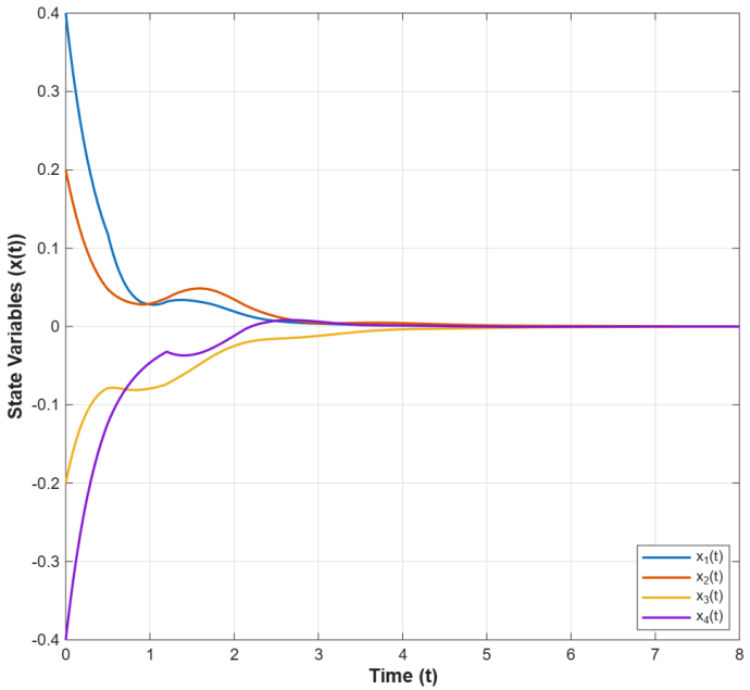
First, let $h_1=0.7$, $h_2=0.15$, $h_3=0.15$, $\kappa =\tilde{\kappa }=\beta =\tilde{\beta }=\eta =\tilde{\eta }=1$, $\widehat{\kappa }=\widehat{\beta }=\widehat{\eta }=0.5$, $k_1=0.3, k_2=0.4, k_3=0.3$, ${\widehat{k}}_1=0.2, {\widehat{k}}_2=0.1, {\widehat{k}}_3=0.7$, ${\tilde{k}}_1=0.4, {\tilde{k}}_2=0.5, {\tilde{k}}_3=0.1$, ${\tau }_1=3, {\tau }_2=5, {\tau }_3=4, {\tau }_4=2$, ${\zeta }_1=11.2, {\zeta }_2=12.8, {\zeta }_3=9.4$ and ${\zeta }_4=15$. The maximum delay bounds for these delays are ${\tau }_M=5$ and ${\zeta }_M=15$ where $\chi =max\{{\tau }_M,{\zeta }_M\}=15$ and the initial condition functions are chosen as follows

$$x\left(t\right)=\left(\begin{array}{c}0.4cos\left(2t\right)+0.3sin\left(2t\right)\\ 0.2cos\left(2t\right)-0.3sin\left(2t\right)\\ -0.2cos\left(2t\right)+0.3sin\left(2t\right)\\ -0.4cos\left(2t\right)-0.3sin\left(2t\right)\end{array}\right),t\in [-15,0]$$

Then, we calculate ${\varrho }_1=3.1238, {\varrho }_2=3.0963, {\varrho }_3=3.0995, {\varrho }_4=3.2789, {\vartheta }_1=0.1510,$${\vartheta }_2=0.1178, {\vartheta }_3=0.1275$ and ${\vartheta }_4=0.2093$. Thus, the stability criteria of Theorem 1 are justified. The time response of neutral system (1) in this case of the example is depicted in Figure 1.

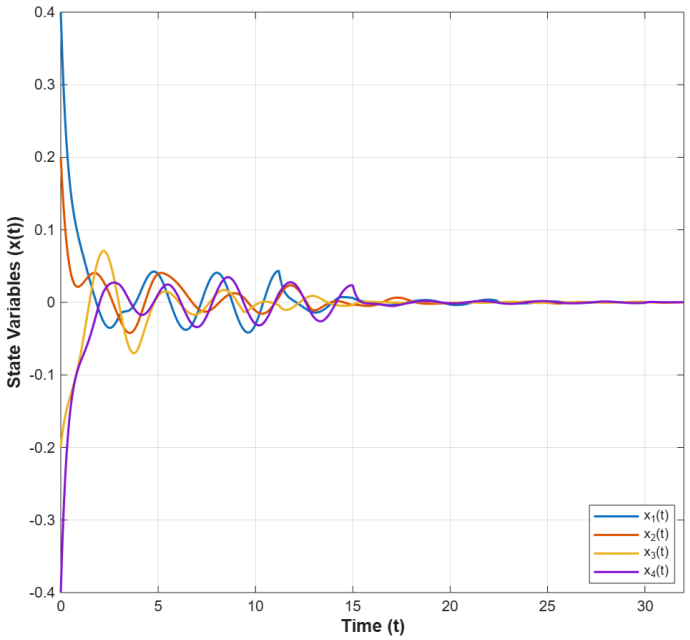
Now, let $h_1=0.7$, $h_2=0.15$, $h_3=0.15$, $\kappa =\tilde{\kappa }=\beta =\tilde{\beta }=\eta =\tilde{\eta }=1$, $\widehat{\kappa }=\widehat{\beta }=\widehat{\eta }=0.5$, $k_1={\widehat{k}}_1={\tilde{k}}_1=1$, ${\tau }_1=3,{\tau }_2=5,{\tau }_3=4,{\tau }_4=2$, ${\zeta }_1=11.2, {\zeta }_2=12.8, {\zeta }_3=9.4$ and ${\zeta }_4=15$. The maximum delay bounds for these delays are ${\tau }_M=5$ and ${\zeta }_M=15$ where $\chi =max\{{\tau }_M,{\zeta }_M\}=15$. We now select the initial conditions of neutral system (1) as follows

$$x\left(t\right)=\left(\begin{array}{c}0.3\\ 0.2\\ -0.2\\ -0.3\end{array}\right),t\in [-15,0]$$

In this case of the example, we also calculate ${\varrho }_1=2.9407, {\varrho }_2=2.9163, {\varrho }_3=2.9191,$${\varrho }_4=3.0785, {\vartheta }_1=0.0724, {\vartheta }_2=0.0335, {\vartheta }_3=0.0455$ and ${\vartheta }_4=0.1363$. Thus, the stability criteria derived in Theorem 1 hold. The time response of neutral system (1) is depicted in Figure 2.

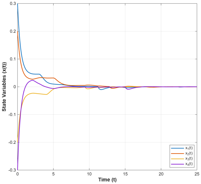
Consider the case where $h_1=1$, $h_2=0$, $h_3=0$, $\kappa =\tilde{\kappa }=\beta =\tilde{\beta }=\eta =\tilde{\eta }=1$, $\widehat{\kappa }=\widehat{\beta }=\widehat{\eta }=0.5$, $k_1={\widehat{k}}_1={\tilde{k}}_1=1$, ${\tau }_1=1.2,{\tau }_2=1.8,{\tau }_3=1.5,{\tau }_4=2.1$, ${\zeta }_1=0.5, {\zeta }_2=0.9, {\zeta }_3=0.7$ and ${\zeta }_4=1.2$. The maximum delay bounds for these delays are ${\tau }_M=2.1$ and ${\zeta }_M=1.2$ where $\chi =max\{{\tau }_M,{\zeta }_M\}=2.1$ and the initial conditions are selected as follows

$$x\left(t\right)=\left(\begin{array}{c}0.3\\ 0.2\\ -0.2\\ -0.3\end{array}\right),t\in [-2.1,0]$$

Then, we calculate ${\varrho }_1=3.6993,{\varrho }_2=3.6728,{\varrho }_3=3.6774,{\varrho }_4=3.8366,{\vartheta }_1=0.6264,$${\vartheta }_2=0.6284,{\vartheta }_3=0.6254$ and ${\vartheta }_4=0.6363$. Thus, the conditions obtained in Theorem 1 hold. For this selection of the parameters, the time response of neutral system given by (1) in this case of the example is depicted in Figure 3.

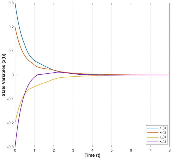
Finally, let $h_1=0$, $h_2=0.5$, $h_3=0.5$, $\kappa =\tilde{\kappa }=\beta =\tilde{\beta }=\eta =\tilde{\eta }=1$, $\widehat{\kappa }=\widehat{\beta }=3$, $\widehat{\eta }=0.5$, $k_1={\widehat{k}}_1={\tilde{k}}_1=1$, ${\tau }_1=1.2,{\tau }_2=1.8,{\tau }_3=1.5,{\tau }_4=2.1$, ${\zeta }_1=0.5, {\zeta }_2=0.9, {\zeta }_3=0.7$ and ${\zeta }_4=1.2$. The maximum delay bounds for these delays are ${\tau }_M=2.1$ and ${\zeta }_M=1.2$ where $\chi =max\{{\tau }_M,{\zeta }_M\}=2.1$ and the initial condition functions are chosen as given below

$$x\left(t\right)=\left(\begin{array}{c}0.4cos\left(2t\right)+0.3sin\left(2t\right)\\ 0.2cos\left(2t\right)-0.3sin\left(2t\right)\\ -0.2cos\left(2t\right)+0.3sin\left(2t\right)\\ -0.4cos\left(2t\right)-0.3sin\left(2t\right)\end{array}\right),t\in [-2.1,0]$$

Then, we calculate ${\varrho }_1=0.9602,{\varrho }_2=0.9420,{\varrho }_3=0.9359,{\varrho }_4=1.1690,{\vartheta }_1=0.1963,$${\vartheta }_2=0.1785,{\vartheta }_3=0.1756$ and ${\vartheta }_4=0.2696$. Consequently, the conditions determined by Theorem 1 are justified. For these parameters of the example, the time response of neutral system defined by (1) is depicted in Figure 4.

5. Conclusions

This article has conducted a theoretical investigation into the stability analysis of neutral-type Cohen–Grossberg neural networks containing discrete time and neutral delay terms. We have established a suitable Lyapunov functional comprising the linear combination of three main Lyapunov functionals of quadratic form. Then, by exploiting this constructed Lyapunov functional, together with some appropriate matrix analysis techniques, novel sufficient conditions for the global asymptotic stability of the neutral neural system have been obtained. The stability conditions are mainly related to the basic network parameters and are independent of the size of the time and neutral delay components. It has been additionally shown that many sets of previously reported stability results associated with different forms of the same neural network can be directly determined from appropriate special cases of the set of Lyapunov functionals employed in this research study. A numerical example, covering different cases of the constructed main Lyapunov functional, has been considered to indicate the applicability of the obtained results. Since employing the appropriate Lyapunov functionals is an essential factor in stability analysis of linear and nonlinear dynamical systems, the analysis techniques and methods used in this paper may lead to some further research in the area of stability theory of various classes of neutral systems. We find it important to note that different models of linear and nonlinear neutral systems can be derived from system (1) by choosing the system functions in some appropriate forms. Then, the Lyapunov functionals proposed in this paper can be further modified for the systems for which the stability analysis will be conducted. The current paper has considered the system with n time delays and n neutral delays. However, the Lyapunov functionals in this paper can be easily used to study the stability of neutral systems with $n^2$ time delays and $n^2$ neutral delays, which would make some important contributions to the previously published results for such systems.

References

1. Cohen, M.; Grossberg, S. Absolute stability of global pattern formation and parallel memory storage by competitive neural networks. IEEE Trans. Syst. Man Cybern. 1983, 13, 815–826. [Google Scholar] [CrossRef] [Scilit]
2. Hopfield, J. Neural networks and physical systems with emergent collective computational abilities. Proc. Natl. Acad. Sci. USA 1982, 79, 2554–2558. [Google Scholar] [CrossRef] [Scilit]
3. Hopfield, J. Neurons with graded response have collective computational properties like those of two-state neurons. Proc. Natl. Acad. Sci. USA 1984, 81, 3088–3092. [Google Scholar] [CrossRef] [Scilit]
4. Kennedy, M.; Chua, L. Neural networks for nonlinear programming. IEEE Trans. Circuits Syst. 1988, 35, 554–562. [Google Scholar] [CrossRef] [Scilit]
5. Pearlmutter, B. Gradient calculations for dynamic recurrent neural networks: A survey. IEEE Trans. Neural Netw. 1995, 6, 1212–1228. [Google Scholar] [CrossRef] [Scilit]
6. Takahashi, Y. A unified constructive network model for problem solving. Theor. Comput. Sci. 1996, 156, 217–261. [Google Scholar] [CrossRef] [Scilit]
7. Tank, D.; Hopfield, J. Simple neural optimization networks: An A/D converter, signal decision circuit, and a linear programming circuit. IEEE Trans. Circuits Syst. 1986, 33, 533–541. [Google Scholar] [CrossRef] [Scilit]
8. Vazquez, A.R.; Castro, R.D.; Rueda, A.; Sinencio, E.S. Nonlinear switched capacitor neural networks for optimization problems. IEEE Trans. Circuits Syst. I 1990, 37, 384–398. [Google Scholar] [CrossRef] [Scilit]
9. Fang, Y.; Kincaid, T.G. Stability analysis of dynamical neural networks. IEEE Trans. Neural Netw. 1996, 7, 996–1006. [Google Scholar] [CrossRef] [Scilit]
10. Qiao, H.; Peng, J.; Xu, Z.B.; Zhang, B. A reference model approach to stability analysis of neural networks. IEEE Trans. Syst. Man Cybern. Part B 2003, 33, 925–936. [Google Scholar] [CrossRef] [Scilit]
11. Rajchakit, G.; Agarwal, P.; Ramalingam, S. Stability Analysis of Neural Networks; Springer Nature: Singapore, 2021. [Google Scholar]
12. Zhang, H.; Wang, Z.; Liu, D. A comprehensive review of stability analysis of continuous-time recurrent neural networks. IEEE Trans. Neural Netw. Learn. Syst. 2014, 25, 1229–1262. [Google Scholar] [CrossRef] [Scilit]
13. Baldi, P.; Atiya, A. How delays affect neural dynamics and learning. IEEE Trans. Neural Netw. 1994, 5, 612–621. [Google Scholar] [CrossRef] [Scilit]
14. Cooke, K.; Grossman, Z. Discrete delay, distributed delay and stability switches. J. Math. Anal. Appl. 1982, 86, 592–627. [Google Scholar] [CrossRef] [Scilit]
15. Marcus, C.; Westervelt, R. Stability of analog neural networks with delay. Phys. Rev. A 1989, 39, 347–359. [Google Scholar] [CrossRef] [Scilit]
16. Aktas, E.; Faydasicok, O.; Arik, S. Robust stability of dynamical neural networks with multiple time delays: A review and new results. Artif. Intell. Rev. 2023, 56, 1647–1684. [Google Scholar] [CrossRef] [Scilit]
17. Arik, S. New criteria for global robust stability of delayed neural networks with norm-bounded uncertainties. IEEE Trans. Neural Netw. Learn. Syst. 2014, 25, 1045–1052. [Google Scholar] [CrossRef] [Scilit]
18. Cao, J.; Huang, D.; Qu, Y. Global robust stability of delayed recurrent neural networks. Chaos Solitons Fractals 2005, 23, 221–229. [Google Scholar] [CrossRef] [Scilit]
19. Chen, Y.; Zhang, N.; Yang, J. A survey of recent advances on stability analysis, state estimation and synchronization control for neural networks. Neurocomputing 2023, 515, 26–36. [Google Scholar] [CrossRef] [Scilit]
20. Du, F.F.; Lu, J.G. New criteria on finite-time stability of fractional-order Hopfield neural networks with time delays. IEEE Trans. Neural Netw. Learn. Syst. 2021, 32, 3858–3866. [Google Scholar] [CrossRef] [Scilit]
21. Lin, H.C.; Zeng, H.B.; Zhang, X.M.; Wang, W. Stability analysis for delayed neural networks via a generalized reciprocally convex inequality. IEEE Trans. Neural Netw. Learn. Syst. 2023, 34, 7491–7499. [Google Scholar] [CrossRef] [Scilit]
22. Wang, H.; Wei, G.; Wen, S.; Huang, T. Generalized norm for existence, uniqueness and stability of Hopfield neural networks with discrete and distributed delays. Neural Netw. 2020, 128, 288–293. [Google Scholar] [CrossRef] [Scilit]
23. Wei, C.; Wang, X.; Hui, M.; Zeng, Z. Quasi-synchronization of fractional multiweighted coupled neural networks via aperiodic intermittent control. IEEE Trans. Cybern. 2024, 54, 1671–1684. [Google Scholar] [CrossRef] [Scilit]
24. Zhang, G.; Cao, J. New results on fixed/predefined-time synchronization of delayed fuzzy inertial discontinuous neural networks. Appl. Math. Comput. 2023, 440, 127671. [Google Scholar] [CrossRef] [Scilit]
25. Kolmanovskii, V.B.; Nosov, V.R. Stability of Functional Differential Equations; Mathematics in Science and Engineering; Academic Press: Cambridge, MA, USA, 1986; Volume 180. [Google Scholar]
26. Shatyrko, A.; van Nooijen, R.R.P.; Kolechkina, A.; Khusainov, D. Stabilization of neutral-type indirect control systems to absolute stability state. Adv. Differ. Equ. 2015, 2015, 64. [Google Scholar] [CrossRef] [Scilit]
27. Kolmanovskii, V.; Myshkis, A. Introduction to the Theory and Applications of Functional-Differential Equations; Mathematics and Its Applications; Kluwer Academic Publishers: Dordrecht, The Netherlands, 1999; Volume 463. [Google Scholar]
28. Chukwu, E.N. Stability and Time-Optimal Control of Hereditary Systems: With Application to the Economic Dynamics of the US; World Scientific: Singapore, 2001. [Google Scholar]
29. Baker, C.T.H.; Bocharov, G.A.; Rihan, F.A. Neutral delay differential equations in the modelling of cell growth. J. Egypt. Math. Soc. 2008, 16, 133–160. [Google Scholar]
30. Chukwu, E.N. Differential Models and Neutral Systems for Controlling the Wealth of Nations; World Scientific: Singapore, 2001. [Google Scholar]
31. Hadeler, K.P.; Bocharov, G. Where to put delays in population models, in particular in the neutral case. Can. Appl. Math. Q. 2003, 11, 159–173. [Google Scholar]
32. Aouiti, C.; Coirault, P.; Miaadi, F.; Moulay, E. Finite time boundedness of neutral high-order Hopfield neural networks with time delay in the leakage term and mixed time delays. Neurocomputing 2017, 260, 378–392. [Google Scholar] [CrossRef] [Scilit]
33. Arik, S. A modified Lyapunov functional with application to stability of neutral-type neural networks with time delays. J. Frankl. Inst. 2019, 356, 276–291. [Google Scholar] [CrossRef] [Scilit]
34. Arik, S. New criteria for stability of neutral-type neural networks with multiple time delays. IEEE Trans. Neural Netw. Learn. Syst. 2020, 31, 1504–1514. [Google Scholar] [CrossRef] [Scilit]
35. Dong, J.; Ma, W. Sufficient conditions for global attractivity of a class of neutral Hopfield-type neural networks. Neurocomputing 2015, 153, 89–95. [Google Scholar] [CrossRef] [Scilit]
36. Faydasicok, O. A new Lyapunov functional for stability analysis of neutral-type Hopfield neural networks with multiple delays. Neural Netw. 2020, 129, 288–297. [Google Scholar] [CrossRef] [Scilit]
37. Li, L.; Li, Y.; Yang, L. Almost periodic solutions for neutral delay Hopfield neural networks with time-varying delays in the leakage term on time scales. Adv. Differ. Equ. 2014, 2014, 178. [Google Scholar] [CrossRef] [Scilit]
38. Li, Y.; Yang, L. Almost automorphic solution for neutral type high-order Hopfield neural networks with delays in leakage terms on time scales. Appl. Math. Comput. 2014, 242, 679–693. [Google Scholar] [CrossRef] [Scilit]
39. Orman, Z. New sufficient conditions for global stability of neutral-type neural networks with time delays. Neurocomputing 2012, 97, 141–148. [Google Scholar] [CrossRef] [Scilit]
40. Skvortsova, M.A. Systems of Neutral Type Equations and a Model of Hopfield Neural Network. Sib. Adv. Math. 2025, 35, 324–342. [Google Scholar] [CrossRef] [Scilit]
41. Wan, L.; Zhou, Q.; Fu, H.; Zhang, Q. Exponential stability of Hopfield neural networks of neutral type with multiple time-varying delays. AIMS Math. 2021, 6, 8030–8043. [Google Scholar] [CrossRef] [Scilit]
42. Wu, F. Global asymptotic stability for neutral-type Hopfield neural networks with multiple delays. J. Phys. Conf. Ser. 2021, 1883, 012089. [Google Scholar] [CrossRef] [Scilit]
43. Zhu, J.; Zhang, Q.; Yang, C. Delay-dependent robust stability for Hopfield neural networks of neutral-type. Neurocomputing 2009, 72, 2609–2617. [Google Scholar] [CrossRef] [Scilit]
44. Akça, H.; Covachev, V.; Covacheva, Z. Global asymptotic stability of Cohen–Grossberg neural networks of neutral type. J. Math. Sci. 2015, 205, 719–728. [Google Scholar] [CrossRef] [Scilit]
45. Arik, S. An analysis of stability of neutral-type neural systems with constant time delays. J. Frankl. Inst. 2014, 351, 4949–4959. [Google Scholar] [CrossRef] [Scilit]
46. Faydasicok, O. New criteria for global stability of neutral-type Cohen–Grossberg neural networks with multiple delays. Neural Netw. 2020, 125, 330–337. [Google Scholar] [CrossRef] [Scilit]
47. Faydasicok, O. New results on stability of delayed Cohen–Grossberg neural networks of neutral type. Complexity 2020, 2020, 1973548. [Google Scholar] [CrossRef] [Scilit]
48. Faydasicok, O. Further stability analysis of neutral-type Cohen–Grossberg neural networks with multiple delays. Discret. Contin. Dyn. Syst.-Ser. S 2021, 14, 1245–1258. [Google Scholar] [CrossRef] [Scilit]
49. Faydasicok, O.; Arik, S. A novel Lyapunov stability analysis of neutral-type Cohen–Grossberg neural networks with multiple delays. Neural Netw. 2022, 155, 330–339. [Google Scholar] [CrossRef] [Scilit]
50. Faydasicok, O.; Arik, S. The combined Lyapunov functionals method for stability analysis of neutral Cohen–Grossberg neural networks with multiple delays. Neural Netw. 2024, 180, 106641. [Google Scholar] [CrossRef] [Scilit]
51. Gan, B.; Chen, H.; Xu, B.; Kang, W. A norm stability condition of neutral-type Cohen–Grossberg neural networks with multiple time delays. Chaos Solitons Fractals 2023, 175, 113958. [Google Scholar] [CrossRef] [Scilit]
52. Jian, J.; Wang, B. Global Lagrange stability for neutral-type Cohen–Grossberg BAM neural networks with mixed time-varying delays. Math. Comput. Simul. 2015, 116, 1–25. [Google Scholar] [CrossRef] [Scilit]
53. Kong, F.; Zhu, Q. New results on global stability analysis of discontinuous Cohen–Grossberg neural networks of neutral-type in Hale’s form. Int. J. Control 2020, 95, 516–525. [Google Scholar] [CrossRef] [Scilit]
54. Ozcan, N. Stability analysis of Cohen–Grossberg neural networks of neutral-type: Multiple delays case. Neural Netw. 2019, 113, 20–27. [Google Scholar] [CrossRef] [Scilit]
55. Samli, R.; Senan, S.; Yucel, E.; Orman, Z. Some generalized global stability criteria for delayed Cohen–Grossberg neural networks of neutral-type. Neural Netw. 2019, 116, 198–207. [Google Scholar] [CrossRef] [Scilit]
56. Sriraman, R.; Rajchakit, G.; Kwon, O.M.; Lee, S.M. Stability analysis for delayed Cohen–Grossberg Clifford-valued neutral-type neural networks. Math. Methods Appl. Sci. 2022, 45, 10925–10945. [Google Scholar] [CrossRef] [Scilit]
57. Wang, L.; Gan, B.; Chen, H. Neutral-Type CGNNs With Multiple Delays: A Frobenius Norm Approach to Stability. IEEE Access 2025, 13, 162845–162854. [Google Scholar] [CrossRef] [Scilit]
58. Zhang, Z.; Liu, W.; Zhou, D. Global asymptotic stability to a generalized Cohen–Grossberg BAM neural networks of neutral type delays. Neural Netw. 2012, 25, 94–105. [Google Scholar] [CrossRef] [Scilit]
59. Zheng, C.D.; Li, J.W.; Wang, Z. New stability criteria for neutral-type Cohen–Grossberg neural networks with discrete and distributed delays. Int. J. Comput. Math. 2012, 89, 443–466. [Google Scholar] [CrossRef] [Scilit]
Figure 1. The time response of states of system (1).
Mathematics 14 03075 g001
Figure 2. The time response of states of system (1).
Mathematics 14 03075 g002
Figure 3. The time response of states of system (1).
Mathematics 14 03075 g003
Figure 4. The time response of system states (1).
Mathematics 14 03075 g004
Disclaimer/Publisher’s Note: The statements, opinions and data contained in all publications are solely those of the individual author(s) and contributor(s) and not of MDPI and/or the editor(s). MDPI and/or the editor(s) disclaim responsibility for any injury to people or property resulting from any ideas, methods, instructions or products referred to in the content.