Adaptive Sparrow Search Algorithm with Dynamic Penalty and Repair Operators for Constrained Disposal Scheduling

Abstract

Solid waste disposal scheduling coordinates waste generation, facility capacities, fleet resources, treatment compatibility, disposal priorities, and environmental costs over multiple periods. The deterministic model considered in this study is a continuous linear program with a convex polyhedral feasible region. To provide a domain-specific population-search framework for this constraint-intensive setting, this paper proposes an Adaptive Sparrow Search Algorithm with Dynamic Penalty and Repair Operators (ADP-SSA). Its distinctive feature is a closed-loop design: population diversity, feasibility ratio, violation type, and stagnation jointly regulate sparrow roles, penalty pressure, and schedule repair. The repair stage performs compatibility correction, capacity redistribution, fleet-resource adjustment, priority-preserving backlog control, terminal clearance, and feasible local refinement. Experiments on six benchmark instances constructed from public New York City and Philadelphia municipal-waste records compare ADP-SSA with SSA, PSO, GA, GWO, and DE under a common evaluation budget. The reported aggregate results indicate lower mean feasible cost and stronger feasibility for ADP-SSA. Friedman and repeated-measures ANOVA tests computed from the six matched instance means identify a global algorithm effect, while exact pairwise Wilcoxon tests are reported with multiplicity correction. The present formulation and evidence do not establish superiority over commercial linear-programming solvers or unexecuted recent optimizers; these comparisons are identified as limitations and priorities for future work.

1. Introduction

Rapid urbanization, changing consumption patterns, and low-carbon service requirements make solid waste disposal scheduling operationally important. Waste generated at communities, sanitation districts, and transfer stations must be assigned to heterogeneous facilities while respecting route compatibility, period-dependent treatment capacity, fleet-resource availability, service priority, and terminal backlog requirements. These decisions couple allocation, capacity, and temporal carry-over rather than forming independent routing choices [1,2,3,4,5].

The model studied here uses continuous flow variables $x_{ijt}$ and backlog variables $b_{it}$. With fixed costs, capacities, compatibility indicators, and resource coefficients, both the objective and constraints are affine; the resulting problem is therefore a linear program with a convex polyhedral feasible region. Its scale grows as $IJT+IT$, and its structure combines adjacent-period flow balance with within-period facility and fleet coupling. This classification is important: commercial linear-programming solvers are appropriate exact methods for the present deterministic model, whereas the proposed metaheuristic is evaluated as a domain-specific constraint-handling framework and as a basis for later mixed-integer, nonlinear, uncertain, and online extensions.

The Sparrow Search Algorithm (SSA) offers a simple discoverer–follower–scout population structure [6]. Existing improvements commonly modify initialization, adaptive weights, perturbation rules, opposition learning, or hybrid local search [7,8,9,10,11,12,13,14,15,16]. These mechanisms can improve generic continuous search, but they do not by themselves preserve multi-period waste balance, treatment compatibility, shared capacities, fleet limits, priority backlog, and terminal clearance. Table 1 makes this distinction explicit.

ADP-SSA addresses this gap through a closed-loop coupling of search and feasibility restoration. A sparrow position ${\mathbf{z}}_n^r$ is decoded into a raw schedule ${\mathbf{X}}_n^r=\mathcal{D}\left({\mathbf{z}}_n^r\right)$, repaired as ${\tilde{\mathbf{X}}}_n^r=\mathcal{R}\left({\mathbf{X}}_n^r\right)$, and evaluated by $F^r\left(\tilde{\mathbf{X}}\right)=C\left(\tilde{\mathbf{X}}\right)+{\lambda }^{r}V\left(\tilde{\mathbf{X}}\right)$. Population diversity, feasibility ratio, violation composition, and stagnation are fed back to role allocation, movement rules, penalty growth, and repair choice. Unlike an isolated adaptive weight or a fixed penalty, the same constraint diagnostics influence exploration, exploitation, and executable schedule recovery. The sequential interaction is summarized in Figure 1.

The contributions are fourfold. First, the paper gives a complete multi-period disposal-flow formulation, proves that the present deterministic continuous model is a linear program, and reports its variable and constraint counts. Second, it develops feasibility-responsive role allocation in which discoverer and scout proportions change with diversity, stagnation, and feasibility. Third, it combines a state-dependent penalty coefficient with priority-preserving repair so that infeasible candidates are differentiated and then corrected according to their dominant violation. Fourth, it provides ablation, sensitivity, aggregate statistical, complexity, parameter-selection, limitation, and scalability analyses.

The experimental study uses six benchmarks constructed from public New York City and Philadelphia municipal-waste records. The reported comparison includes standard SSA, Particle Swarm Optimization, Genetic Algorithm, Grey Wolf Optimizer, and Differential Evolution, with best and mean feasible cost, standard deviation, feasibility rate, ablation behavior, sensitivity, and convergence indicators. Section 2 reviews the relevant literature; Section 3 presents the model and its structure; Section 4 describes ADP-SSA; Section 5 reports the available experiments and statistical analyses; and Section 6 and Section 7 discuss limitations, future scope, and conclusions.

2. Related Work

2.1. Solid Waste Logistics and Disposal Scheduling

Solid waste management has long been studied as an operations research problem involving facility location, waste allocation, collection routing, transfer planning, and treatment scheduling. Ghiani et al. reviewed strategic and tactical optimization issues in solid waste management and showed that cost, capacity, service frequency, and facility selection are often coupled rather than separable decisions [1]. More recently, Alshaikh and Abdelfatah provided a systematic review of optimization techniques in municipal solid waste management, emphasizing that modern urban waste systems require integrated models rather than isolated routing or facility-location modules [2]. Thakur et al. further examined meta-heuristic approaches for waste-management routing problems and reported that swarm intelligence and evolutionary computation remain attractive when exact optimization becomes computationally expensive [3]. These studies provide the broader background for the constrained disposal scheduling problem considered in this paper, where the decision tensor $\mathbf{X}=\left[x_{ijt}\right]$ must simultaneously satisfy waste-flow balance, facility capacity, fleet-resource availability, and terminal disposal requirements.

Recent waste-logistics studies have moved toward more realistic operating constraints. Ferrão et al. developed an algorithmic route-optimization application for municipal waste collection and showed that route-level optimization can reduce unnecessary travel while maintaining service coverage [4]. Silva et al. investigated hybrid fleet optimization for waste collection under urban constraints using OR-Tools, highlighting the importance of vehicle heterogeneity and operational restrictions in practical waste services [5]. In addition to routing, energy-related waste and resource scheduling has also attracted attention. Liu et al. studied economic scheduling for a new-energy hydrogen-synthesis-ammonia system using a sparrow-search-based optimization method, indicating that swarm intelligence can be adapted to resource-dispatching problems with coupled operational constraints [17]. However, most existing waste-routing studies mainly optimize vehicle paths or collection sequences, while fewer works explicitly model multi-period disposal flows from generation nodes to heterogeneous treatment facilities. The present study differs from these works by optimizing $x_{ijt}$ over the whole planning horizon $\mathcal{T}$ and by directly incorporating backlog $b_{it}$, facility capacity $U_{jt}$, fleet resource $R_t$, and priority coefficient ${\rho }_i$ into the scheduling model [18,19,20].

2.2. Sparrow Search and Adaptive Swarm Optimization

The Sparrow Search Algorithm was originally proposed by Xue and Shen as a swarm intelligence optimizer inspired by sparrow foraging and anti-predation behaviors [6]. Its population structure based on discoverers, followers, and scouts provides a concise search mechanism, but the original algorithm can still suffer from premature convergence, insufficient diversity, and weak constraint-handling ability when applied to complex scheduling spaces. To address these limitations, many recent studies have enhanced SSA through chaotic initialization, adaptive weights, multi-strategy perturbation, opposition learning, and hybrid local search. He and Wang introduced an improved chaos SSA for unmanned aerial vehicle path planning, showing that chaotic search can strengthen population diversity in path-optimization scenarios [7]. Hou et al. integrated an improved SSA with the dynamic window approach for mobile-robot path planning, demonstrating that SSA can be combined with domain-specific feasibility rules [8]. Xu, Sang, and Zhang applied an improved SSA to mobile-robot path planning and further confirmed its applicability to constrained trajectory generation [9]. Ma et al. studied industrial robot trajectory optimization based on an improved SSA, reflecting the growing use of SSA variants in engineering scheduling and motion-planning problems [10].

Other recent studies focus on strengthening the core search dynamics of SSA. Hu and Wang proposed an improved SSA and investigated its research application, showing that adaptive improvements can enhance convergence stability [11]. Li et al. combined an improved SSA with a CNN-BiLSTM network for sea-level prediction, indicating that SSA can also act as a parameter-optimization tool in prediction models [12]. Yang et al. proposed an enhanced SSA based on an improved game predatory mechanism and applied it to digital-signal-processing tasks, where adaptive competition improves global search behavior [13]. Xu et al. developed a multi-strategy collaborative improved SSA and applied it to path planning, suggesting that no single perturbation mechanism is sufficient for all search stages [14]. Wang et al. proposed a multi-strategy integrated improved SSA, providing further evidence that adaptive and hybrid mechanisms can improve the balance between exploration and exploitation [15]. Ma et al. incorporated multiple strategies into a modified SSA for mathematical optimization problems, demonstrating competitive performance on benchmark functions [16]. Although these methods improve SSA from different perspectives, they are mostly designed for continuous benchmarks, forecasting models, or path-planning tasks. They do not directly address the tensor-encoded disposal schedule $\mathbf{X}$, the dynamic penalty coefficient ${\lambda }^r$, or the priority-preserving repair operator $\mathcal{R}(·)$ required by constrained multi-period waste disposal scheduling.

The central methodological distinction is summarized in Table 1. Existing adaptive SSA families mainly alter population initialization or movement equations, whereas ADP-SSA also uses feasibility information to change role proportions, penalty pressure, and domain-specific repair within one feedback loop.

Table 1. Positioning of ADP-SSA relative to representative SSA families. A check mark indicates that the feature is an explicit algorithmic component rather than an external feasibility filter.

Method Family	Adaptive Role Proportions	Feasibility Feedback	Dynamic Penalty	Domain-Specific Repair	Multi-Period Tensor Encoding
Standard SSA [6]	No	No	No	No	No
Chaos/adaptive-weight SSA [7,11]	Partial	No	No	No	No
Multi-strategy SSA [14,15,16]	Partial	No	No	No	No
ADP-SSA	Yes	Yes	Yes	Yes	Yes

Table 1. Positioning of ADP-SSA relative to representative SSA families. A check mark indicates that the feature is an explicit algorithmic component rather than an external feasibility filter.

Method Family	Adaptive Role Proportions	Feasibility Feedback	Dynamic Penalty	Domain-Specific Repair	Multi-Period Tensor Encoding
Standard SSA [6]	No	No	No	No	No
Chaos/adaptive-weight SSA [7,11]	Partial	No	No	No	No
Multi-strategy SSA [14,15,16]	Partial	No	No	No	No
ADP-SSA	Yes	Yes	Yes	Yes	Yes

2.3. Constraint Handling in Metaheuristic Scheduling

Constraint handling is a central issue when metaheuristic algorithms are applied to real scheduling problems. Deb proposed an efficient constraint-handling method for genetic algorithms based on feasibility–priority comparison, which remains influential because it avoids excessive dependence on manually tuned static penalties [21]. In recent engineering scheduling, adaptive constraint strategies have continued to receive attention. He et al. developed a hybrid reservoir scheduling optimization method that couples an adaptive $\epsilon$-constraint mechanism with multi-strategy optimization, showing that constraint pressure should vary with the state of the search process rather than remain fixed [22]. Opposition-based learning has also been widely used to improve population diversity and initialization quality in metaheuristic search, as reviewed by Mahdavi et al. [23]. These works motivate the design of ADP-SSA, in which $F^r\left(\mathbf{X}\right)=C\left(\mathbf{X}\right)+{\lambda }^{r}V\left(\mathbf{X}\right)$ uses a dynamic penalty coefficient ${\lambda }^r$ and the violation profile $\mathbf{v}\left(\mathbf{X}\right)$ is fed back into role allocation, scout movement, and repair selection.

Recent 2026 optimization studies reinforce the value of model-aware constraint treatment but address different problem classes. Li, Zhang, and Shi reformulate distributionally robust stochastic model predictive control with chance constraints into tractable expressions and combine it with self-triggered updating [24]. Feng et al. use second-order iterative optimization and adaptive robust regularization to improve convergence under large perturbations in cross-view localization [25]. Zheng et al. optimize coupled primary and backup service-function paths under latency and reliability requirements [26]. These studies illustrate three current directions—tractable reformulation, iteration-aware robustness, and application-specific constraint structure. ADP-SSA differs by coupling feasibility diagnostics with adaptive swarm roles, a dynamic penalty, and schedule-specific repair for multi-period disposal flows; the cited methods are therefore used for technical positioning rather than treated as directly executable benchmark competitors.

Classical metaheuristic baselines provide important comparison points for constrained disposal scheduling. Particle Swarm Optimization introduced population-level velocity learning and remains widely used for continuous optimization [27]. Differential Evolution uses mutation and recombination among candidate vectors and is effective for many numerical optimization problems [28]. Grey Wolf Optimizer simulates the leadership hierarchy and hunting behavior of gray wolves, offering a simple exploitation-oriented swarm mechanism [29]. Nevertheless, these algorithms do not inherently preserve waste-flow balance, route compatibility, facility capacity, fleet-resource feasibility, or terminal backlog clearance. In the disposal scheduling problem formulated in Section 3, a candidate solution may have low direct cost $C\left(\mathbf{X}\right)$ but still be infeasible because $V_{\mathrm{cap}}\left(\mathbf{X}\right)$, $V_{\mathrm{fleet}}\left(\mathbf{X}\right)$, or $V_{\mathrm{term}}\left(\mathbf{X}\right)$ is nonzero. The proposed ADP-SSA addresses this gap by combining adaptive SSA search dynamics with dynamic penalty evaluation and a priority-preserving repair operator. This combination enables the algorithm to search beyond a narrow feasible region in early iterations while still converging toward executable schedules with $V\left({\mathbf{X}}^{★}\right)=0$.

3. Preliminaries

3.1. Constrained Disposal Scheduling Setting

This study considers a multi-period solid waste disposal scheduling problem in which waste generated from multiple urban sources must be transported to compatible disposal or treatment facilities under capacity, fleet-resource, route-availability, and priority constraints. Let $\mathcal{I}=\{1,2,\dots ,I\}$ denote the set of waste generation nodes, such as communities, collection stations, or transfer stations, and let $\mathcal{J}=\{1,2,\dots ,J\}$ denote the set of disposal facilities, including landfills, incineration plants, recycling centers, composting facilities, and other treatment sites. The scheduling horizon is divided into $\mathcal{T}=\{1,2,\dots ,T\}$ discrete periods. For each node $i\in \mathcal{I}$ and period $t\in \mathcal{T}$, $q_{it}$ denotes the amount of newly generated waste. The binary parameter $a_{ij}$ indicates whether waste from node i can be transported to facility j, where $a_{ij}=1$ means that the route and treatment type are available and $a_{ij}=0$ means that the assignment is forbidden.

The main decision variable is $x_{ijt}$, which represents the amount of waste transported from node i to facility j during period t. Because not all waste is necessarily processed immediately when the system is congested, $b_{it}$ is introduced as the remaining backlog of node i at the end of period t. The initial backlog is denoted by $b_{i0}$, and it is usually set to 0 when no untreated waste remains before the planning horizon. Each facility j has an available disposal capacity $U_{jt}$ in period t, while the total fleet service resource in period t is denoted by $R_t$. The parameter ${\tau }_{ij}$ denotes the unit fleet-resource consumption for transporting waste from node i to facility j, which may represent normalized vehicle-hours, loading effort, or transportation time per tonne. The priority coefficient of node i is denoted by ${\rho }_i$, where a larger ${\rho }_i$ indicates higher urgency and therefore a lower tolerance for delayed disposal. The parameter $B_i^{\max }$ is the maximum allowable backlog at node i, and $\gamma$ is the coefficient that converts priority-weighted backlog into the objective scale.

The scheduling objective considers both economic and environmental costs. The transportation distance between node i and facility j is $d_{ij}$, the unit transportation cost is $c_{ij}^{\mathrm{tr}}$, the unit treatment cost at facility j is $c_j^{\mathrm{op}}$, the unit transportation emission factor is ${ϵ}_{ij}^{\mathrm{tr}}$, and the unit facility-processing emission factor is ${ϵ}_j^{\mathrm{op}}$. The carbon conversion coefficient is denoted by $\eta$, which converts emissions into the same monetary scale as the operating cost. Therefore, the unit generalized disposal cost from node i to facility j is defined as $g_{ij}=c_{ij}^{\mathrm{tr}}{d}_{ij}+c_j^{\mathrm{op}}+\eta ({ϵ}_{ij}^{\mathrm{tr}}{d}_{ij}+{ϵ}_j^{\mathrm{op}})$. This definition allows the subsequent model and algorithm to evaluate each candidate schedule with a unified cost measure while still retaining the physical meaning of transportation cost, facility operation cost, and carbon-emission burden.

3.2. Mathematical Formulation

A candidate schedule is represented by $\mathbf{X}={\left[x_{ijt}\right]}_{I\times J\times T}$, and $\mathbf{b}={\left[b_{it}\right]}_{I\times T}$ records end-of-period backlog. The initial value $b_{i0}$ is a fixed parameter. With the generalized unit cost $g_{ij}$ defined in Section 3.1, the complete deterministic model is

$$\begin{array}{cccc}\hfill \underset{\mathbf{X},\mathbf{b}}{\min }& \sum _{t\in \mathcal{T}}\sum _{i\in \mathcal{I}}\sum _{j\in \mathcal{J}}{g}_{ij}{x}_{ijt}+\gamma \sum _{t\in \mathcal{T}}\sum _{i\in \mathcal{I}}{\rho }_i{b}_{it}\hfill & \hfill & \hfill \\ \hfill \mathrm{s}.\mathrm{t}.& b_{it}=b_{i,t-1}+q_{it}-\sum _{j\in \mathcal{J}}{x}_{ijt},\hfill & \hfill & i\in \mathcal{I},t\in \mathcal{T},\hfill \\ \hfill & x_{ijt}\le a_{ij}\left(b_{i,t-1}+q_{it}\right),\hfill & \hfill & i\in \mathcal{I},j\in \mathcal{J},t\in \mathcal{T},\hfill \\ \hfill & \sum _{i\in \mathcal{I}}{x}_{ijt}\le U_{jt},\hfill & \hfill & j\in \mathcal{J},t\in \mathcal{T},\hfill \\ \hfill & \sum _{i\in \mathcal{I}}\sum _{j\in \mathcal{J}}{\tau }_{ij}{x}_{ijt}\le R_t,\hfill & \hfill & t\in \mathcal{T},\hfill \\ \hfill & 0\le b_{it}\le B_i^{\max },\hfill & \hfill & i\in \mathcal{I},t\in \mathcal{T},\hfill \\ \hfill & b_{iT}=0,\hfill & \hfill & i\in \mathcal{I},\hfill \\ \hfill & x_{ijt}\ge 0,\hfill & \hfill & i\in \mathcal{I},j\in \mathcal{J},t\in \mathcal{T}.\hfill \end{array}$$

(1)

The flow-balance equations propagate backlog across adjacent periods. The compatibility inequalities set $x_{ijt}=0$ whenever $a_{ij}=0$ and otherwise limit each arc by the waste available at its source. Facility and fleet inequalities couple all source nodes within the same period, the backlog bounds encode service priority, and the terminal equalities prohibit disposal from being deferred beyond the horizon. The frequently written availability constraint ${\sum }_j{x}_{ijt}\le b_{i,t-1}+q_{it}$ is implied by flow balance and $b_{it}\ge 0$, so it is omitted from Equation (1) to avoid a redundant row.

For constraint-aware search, let ${\left[z\right]}_{+}=\max (0,z)$ and define

$$V\left(\mathbf{X}\right)={\omega }_1{V}_{\mathrm{flow}}\left(\mathbf{X}\right)+{\omega }_2{V}_{\mathrm{cap}}\left(\mathbf{X}\right)+{\omega }_3{V}_{\mathrm{fleet}}\left(\mathbf{X}\right)+{\omega }_4{V}_{\mathrm{pri}}\left(\mathbf{X}\right)+{\omega }_5{V}_{\mathrm{term}}\left(\mathbf{X}\right).$$

(2)

Here $V_{\mathrm{flow}}$ measures violations of the balance equations and nonnegative availability; $V_{\mathrm{cap}}={\sum }_{t,j}{[{\sum }_i{x}_{ijt}-U_{jt}]}_{+}$; $V_{\mathrm{fleet}}={\sum }_t{[{\sum }_{i,j}{\tau }_{ij}{x}_{ijt}-R_t]}_{+}$; $V_{\mathrm{pri}}={\sum }_{t,i}{[b_{it}-B_i^{\max }]}_{+}$; and $V_{\mathrm{term}}={\sum }_i{b}_{iT}$. The weights ${\omega }_1,\dots ,{\omega }_5$ normalize the components. A schedule is feasible when $V\left(\mathbf{X}\right)=0$.

3.3. Convexity, Size, and Constraint Structure

All quantities $q_{it}$, $a_{ij}$, $U_{jt}$, $R_t$, ${\tau }_{ij}$, $B_i^{\max }$, $g_{ij}$, ${\rho }_i$, and $b_{i0}$ are fixed parameters. Equation (1) has a linear objective and affine equalities and inequalities; consequently, its feasible set $\mathsf{\Omega }$ is a convex polyhedron and the present deterministic continuous problem is a linear program. It contains no intrinsic non-convexity. Non-convexity would arise only after extensions such as binary facility activation, integer vehicle counts, discrete route selection, nonlinear congestion or emission functions, or endogenous compatibility decisions.

In the dense formulation, the numbers of flow and backlog variables are $IJT$ and $IT$, respectively, giving $IT(J+1)$ variables. Excluding variable bounds, there are $IT+I$ equality rows and $IJT+JT+T+IT$ inequality rows. These counts are upper bounds because variables on incompatible arcs can be removed before solution.

Table 2. Dense linear-programming dimensions of the six benchmark instances. Structural rows exclude nonnegativity and simple variable bounds.

Instance	x Variables	b Variables	Total Variables	Equality Rows	Inequality Rows	Total Rows
NYC-S	756	126	882	144	931	1075
NYC-M	3920	490	4410	525	4536	5061
NYC-L	17,700	1770	19,470	1829	19,800	21,629
PHL-S	420	84	504	96	546	642
PHL-M	2352	336	2688	360	2800	3160
PHL-L	12,420	1380	13,800	1426	14,100	15,526

reports the dense dimensions of every benchmark and makes the term “large-scale” precise in this paper.

The constraint matrix has a sparse block-angular and block-banded structure. Arc costs and compatibility are separable by $(i,j,t)$; facility and fleet rows couple nodes only within the same period; and temporal coupling enters through the first-order backlog recursion. This structure supports incremental feasibility checks in the repair operator and also provides several exact or decomposition-based alternatives.

3.4. Exact-Solver Positioning and Decomposition Opportunities

The largest dense model in Table 2 has 19,470 variables and 21,629 structural rows, a size that is generally within the intended range of modern linear-programming solvers. Accordingly, no claim is made that a commercial solver fails at any reported benchmark dimension. Exact simplex or interior-point solutions would provide optimal objective values and valid optimality gaps for the current deterministic model. The available archive does not contain solver logs or the complete numerical instance matrices; consequently, an exact-solver comparison is not reported and this evidence gap is stated in Section 6.

For larger or extended models, the structure permits decomposition without changing the physical interpretation. Dualizing facility-capacity and fleet-resource rows decomposes the remaining problem by source node, with multipliers coordinating shared resources. A rolling-horizon scheme decomposes by time while retaining one or more overlap periods to preserve backlog continuity. Nodes with similar compatibility sets, unit costs, and priority coefficients can be aggregated, solved at cluster level, and disaggregated by residual-capacity rules. Dantzig–Wolfe or column-generation methods are natural when feasible node schedules are treated as columns, while Benders decomposition becomes more relevant after binary facility or vehicle decisions are introduced. These exact and hybrid approaches complement, rather than contradict, the population-based framework.

3.5. Sparrow Search Representation and Constraint Handling Basis

The Sparrow Search Algorithm is a population-based metaheuristic inspired by the foraging and anti-predation behaviors of sparrow groups. In the present scheduling problem, each sparrow represents one candidate disposal schedule. Because the original sparrow position is usually encoded as a continuous vector, the position of sparrow n at iteration r is denoted by ${\mathbf{z}}_n^r$, and a decoding function $\mathcal{D}(·)$ maps it into a disposal schedule ${\mathbf{X}}_n^r=\mathcal{D}\left({\mathbf{z}}_n^r\right)$. The vector ${\mathbf{z}}_n^r$ has dimension $I\times J\times T$ and is reshaped into the tensor form required by ${\mathbf{X}}_n^r$. During decoding, larger position values indicate stronger assignment preference, but the actual dispatched quantities are determined together with waste availability, facility capacity, and compatibility conditions.

At each iteration, the population is divided into discoverers, followers, and scouts. Discoverers are responsible for exploring promising regions of the search space, followers update their positions according to superior individuals, and scouts help the population avoid dangerous or stagnant regions. Let ${\mathcal{D}}_{\mathrm{s}}^r$, ${\mathcal{F}}_{\mathrm{s}}^r$, and ${\mathcal{S}}_{\mathrm{s}}^r$ denote the discoverer, follower, and scout subsets at iteration r, respectively. The subscript $\mathrm{s}$ is used only to distinguish these sparrow-role sets from the decoding function $\mathcal{D}(·)$. In the proposed paper, these role sets are not fixed. Their sizes and update behaviors are adjusted according to convergence status, population diversity, and infeasibility level, which prepares the basis for the adaptive search strategy developed in Section 4.

Constraint handling is essential because the decoded schedule ${\mathbf{X}}_n^r$ may violate facility capacities, fleet resources, route compatibility, or terminal disposal requirements. To evaluate both feasible and infeasible schedules during the search, a penalized fitness function is introduced as $F^r\left(\mathbf{X}\right)=C\left(\mathbf{X}\right)+{\lambda }^{r}V\left(\mathbf{X}\right)$, where ${\lambda }^r$ is the dynamic penalty coefficient at iteration r. A small ${\lambda }^r$ allows the population to explore infeasible but potentially useful regions in the early stage, while a larger ${\lambda }^r$ forces the population toward feasible high-quality schedules in later iterations. In addition, a repair operator $\mathcal{R}(·)$ is used to transform a decoded schedule into a corrected schedule $\tilde{\mathbf{X}}=\mathcal{R}\left(\mathbf{X}\right)$ by redistributing overloaded facility inflows, reducing fleet-resource excess, preserving high-priority disposal, and clearing terminal backlog whenever feasible. The final evaluated solution of sparrow n at iteration r is therefore written as ${\tilde{\mathbf{X}}}_n^r=\mathcal{R}\left(\mathcal{D}\left({\mathbf{z}}_n^r\right)\right)$. This representation establishes a unified connection between the mathematical model and the adaptive sparrow search procedure used in the following sections.

4. Methodology

4.1. Overall Framework and Schedule Encoding

This section presents the proposed Adaptive Sparrow Search with Dynamic Penalty and Repair Operators, abbreviated as ADP-SSA, for solving the constrained disposal scheduling model formulated in Section 3. The central idea of ADP-SSA is to search in a continuous preference space while evaluating candidate solutions in the original constrained scheduling space. Each sparrow position ${\mathbf{z}}_n^r$ is first decoded into a raw disposal schedule ${\mathbf{X}}_n^r=\mathcal{D}\left({\mathbf{z}}_n^r\right)$, then corrected by the repair operator as ${\tilde{\mathbf{X}}}_n^r=\mathcal{R}\left({\mathbf{X}}_n^r\right)$, and finally evaluated by the dynamic penalized fitness function $F^r\left({\tilde{\mathbf{X}}}_n^r\right)=C\left({\tilde{\mathbf{X}}}_n^r\right)+{\lambda }^{r}V\left({\tilde{\mathbf{X}}}_n^r\right)$. This design separates search behavior from feasibility enforcement. The continuous sparrow position preserves the flexibility of swarm-based global exploration, while the decoded and repaired schedule directly satisfies, or approaches, the practical constraints of disposal operations.

For a population with N sparrows, the position of sparrow n at iteration r is encoded as ${\mathbf{z}}_n^r\in {\mathbb{R}}^{I\times J\times T}$. The element $z_{n,ijt}^r$ represents the assignment preference of sending waste from generation node i to facility j during period t. A larger value of $z_{n,ijt}^r$ means that the pair $(i,j)$ is more likely to receive a larger portion of the available waste of node i in period t, but it does not directly determine the final transported amount because the actual schedule must also respect route compatibility, facility capacity, fleet resources, and backlog evolution. To avoid assigning waste to unavailable routes, the decoding procedure first masks incompatible links by setting the effective preference of $(i,j)$ to zero whenever $a_{ij}=0$. For compatible links, the preference is normalized within each pair of node and period. The normalized assignment ratio is computed as $p_{n,ijt}^r=a_{ij}\exp \left(z_{n,ijt}^r\right)/{\sum }_{k\in \mathcal{J}}{a}_{ik}\exp \left(z_{n,ikt}^r\right)$ when at least one compatible facility exists for node i; otherwise, all corresponding ratios are set to zero and the generated waste remains as backlog. This softmax-style decoding keeps $p_{n,ijt}^r$ nonnegative and ensures ${\sum }_{j\in \mathcal{J}}{p}_{n,ijt}^r=1$ over compatible facilities.

Given the normalized preference $p_{n,ijt}^r$, the raw dispatched amount is initially generated as $x_{n,ijt}^{r,0}=p_{n,ijt}^r(b_{i,t-1}^{r,0}+q_{it})$, where $b_{i,t-1}^{r,0}$ is the provisional backlog before period t in the raw decoding stage. This step guarantees that the total outgoing waste from node i does not exceed the amount available at the beginning of period t. However, because different nodes are decoded simultaneously, the provisional schedule may still violate facility capacity or fleet-resource constraints after the flows of all nodes are aggregated. Therefore, the raw tensor ${\mathbf{X}}_n^{r,0}=\left[x_{n,ijt}^{r,0}\right]$ is not directly used as the final candidate schedule. Instead, it is passed to the repair operator developed later in this section, which performs capacity redistribution, fleet-resource correction, and terminal backlog clearance while preserving the priority structure of waste nodes.

The proposed encoding has three advantages for constrained disposal scheduling. First, it avoids discrete assignment instability. Directly representing facility choices as integer variables often causes abrupt changes in the schedule when a sparrow position is updated, whereas the continuous preference representation allows gradual adjustment of allocation ratios. Second, it naturally supports multi-period coupling. Since ${\mathbf{z}}_n^r$ contains all elements $z_{n,ijt}^r$ over the complete horizon $\mathcal{T}$, the algorithm can modify early-period and late-period dispatching decisions jointly rather than optimizing each period independently. Third, it provides a unified interface for adaptive swarm updates. Discoverers, followers, and scouts all update their positions in the same continuous space, while the decoding and repair procedures ensure that the resulting solution remains interpretable as a practical disposal schedule.

The whole ADP-SSA procedure can be described as a repeated transformation from preference search to feasible scheduling. At the beginning, the initial population ${\left\{{\mathbf{z}}_n^0\right\}}_{n=1}^N$ is generated using a hybrid initialization scheme. Part of the population is sampled uniformly to maintain diversity, while the remaining individuals are initialized according to a cost-priority heuristic in which lower-cost and lower-emission facilities receive larger initial preferences. This hybrid initialization improves the chance of locating promising regions early without forcing the population to start from a narrow deterministic pattern. At each iteration, the role sets ${\mathcal{D}}_{\mathrm{s}}^r$, ${\mathcal{F}}_{\mathrm{s}}^r$, and ${\mathcal{S}}_{\mathrm{s}}^r$ are determined adaptively according to the current population diversity and feasibility ratio. The position of each sparrow is then updated according to its role, decoded into ${\mathbf{X}}_n^r$, repaired into ${\tilde{\mathbf{X}}}_n^r$, and evaluated by $F^r\left({\tilde{\mathbf{X}}}_n^r\right)$. The best schedule found so far is recorded as ${\mathbf{X}}^{★}$, and the corresponding objective value is denoted by $C\left({\mathbf{X}}^{★}\right)$ when ${\mathbf{X}}^{★}$ is feasible.

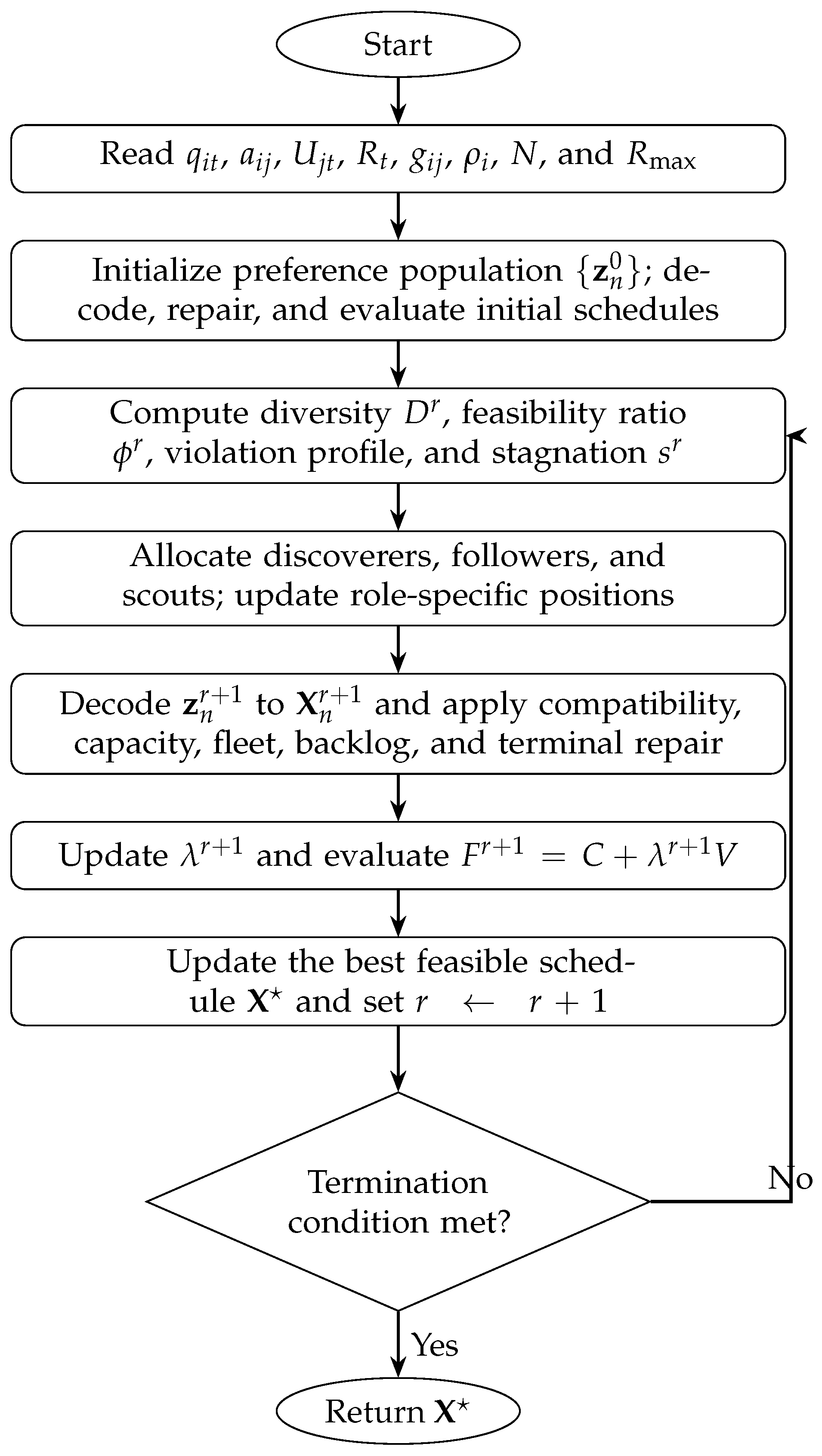
Algorithm 1 summarizes the main computational flow. The later subsections describe the adaptive role update, the dynamic penalty mechanism, and the repair operators in detail. In this framework, the termination condition can be a maximum iteration number $R_{\max }$, a maximum number of consecutive non-improving iterations, or convergence of the best feasible objective value. In the experiments of Section 5, the maximum iteration criterion is used to ensure fair comparison among different algorithms.

Algorithm 1 Overall framework of ADP-SSA for constrained disposal scheduling

1: Input: Sets $\mathcal{I}$, $\mathcal{J}$, and $\mathcal{T}$; waste generation $q_{it}$; compatibility $a_{ij}$; capacity $U_{jt}$; fleet resource $R_t$; cost parameter $g_{ij}$; priority coefficient ${\rho }_i$; maximum iteration $R_{\max }$; population size N.   2: Output: Best feasible disposal schedule ${\mathbf{X}}^{★}$.   3: Initialize sparrow positions ${\left\{{\mathbf{z}}_n^0\right\}}_{n=1}^N$ using hybrid random and cost-priority initialization.   4: Decode each ${\mathbf{z}}_n^0$ into ${\mathbf{X}}_n^0=\mathcal{D}\left({\mathbf{z}}_n^0\right)$ and repair it as ${\tilde{\mathbf{X}}}_n^0=\mathcal{R}\left({\mathbf{X}}_n^0\right)$.   5: Evaluate each repaired schedule by $F^0({\tilde{\mathbf{X}}}_n^0)=C({\tilde{\mathbf{X}}}_n^0)+{\lambda }^{0}V({\tilde{\mathbf{X}}}_n^0)$ and record the best feasible schedule ${\mathbf{X}}^{★}$.   6: for $r=1$ to $R_{\max }$ do   7:     Compute the population diversity, feasibility ratio, and convergence indicator.   8:     Adaptively determine the discoverer set ${\mathcal{D}}_{\mathrm{s}}^r$, follower set ${\mathcal{F}}_{\mathrm{s}}^r$, and scout set ${\mathcal{S}}_{\mathrm{s}}^r$.   9:     Update sparrow positions according to their roles in the continuous preference space. 10:     Decode updated positions into raw schedules and apply repair operators to obtain ${\left\{{\tilde{\mathbf{X}}}_n^r\right\}}_{n=1}^N$. 11:     Update the dynamic penalty coefficient ${\lambda }^r$ and evaluate all repaired schedules by $F^r(·)$. 12:     Update ${\mathbf{X}}^{★}$ if a feasible schedule with a lower value of $C(·)$ is obtained. 13: end for 14: Return ${\mathbf{X}}^{★}$.

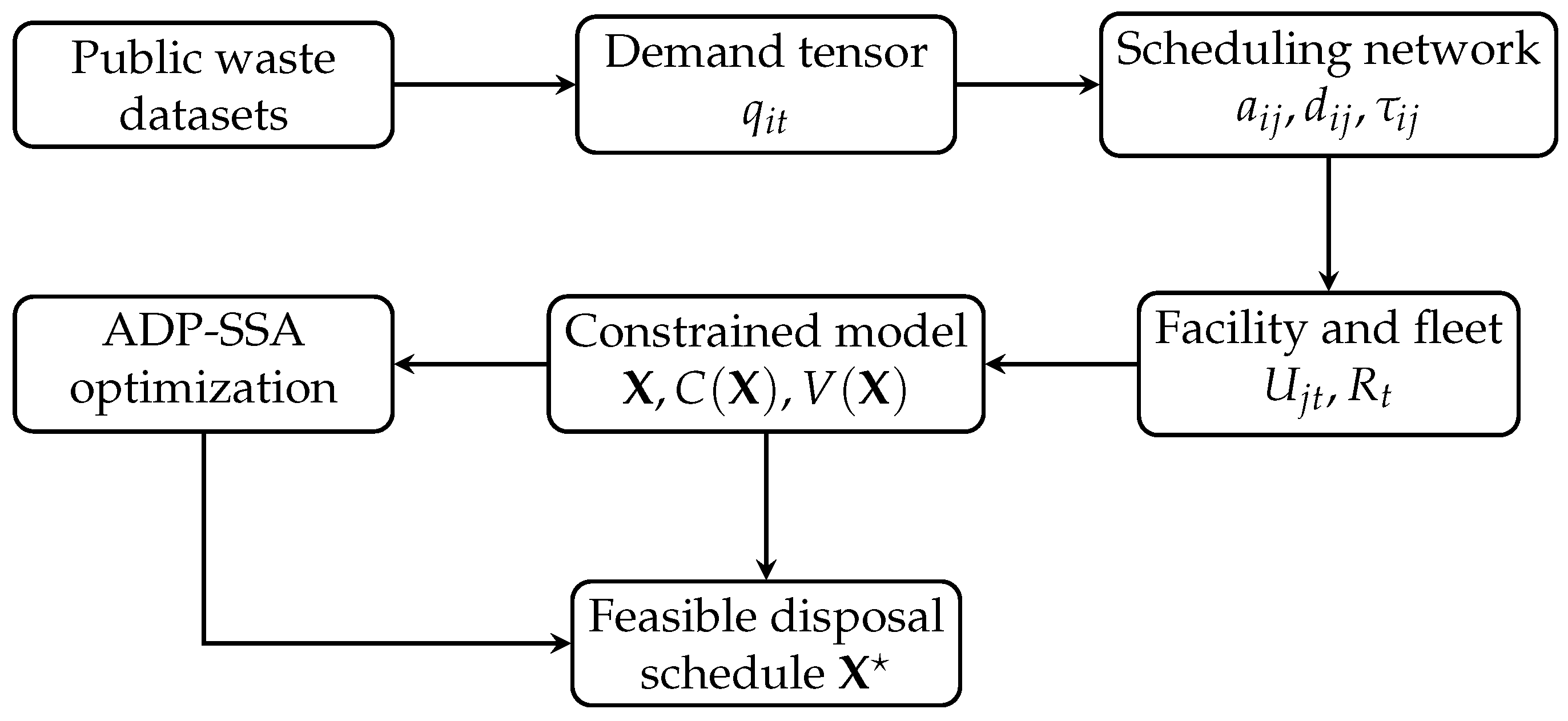
Figure 1 gives a schematic view of the sequential decisions in Algorithm 1. The loop makes explicit that feasibility diagnostics are recomputed before role allocation and that decoding, repair, and dynamic-penalty evaluation occur before the best schedule is updated.

4.2. Adaptive Role Allocation and Search Dynamics

The standard Sparrow Search Algorithm usually assigns fixed proportions of discoverers, followers, and scouts during the whole search process. Such a fixed-role mechanism is not sufficiently flexible for constrained disposal scheduling because the population may face different optimization requirements at different stages. In the early stage, broad exploration is needed to identify promising disposal patterns across facilities and periods. In the middle stage, the algorithm must compare alternative waste-flow structures and reduce unnecessary transportation and treatment costs. In the late stage, the search should concentrate on feasible neighborhoods of high-quality schedules and avoid destroying already feasible assignments. Therefore, ADP-SSA adaptively updates both the role proportions and the position dynamics of sparrows according to population diversity, feasibility ratio, and convergence status.

At iteration r, the population diversity is measured in the continuous preference space. Let ${\overline{\mathbf{z}}}^r=(1/N){\sum }_{n=1}^N{\mathbf{z}}_n^r$ denote the population centroid. The diversity indicator is defined as

$$D^r={\displaystyle \frac{1}{N}}{\displaystyle \sum _{n=1}^N}{\displaystyle \frac{\parallel {\mathbf{z}}_n^r-{\overline{\mathbf{z}}}^r{\parallel }_2}{\parallel {\overline{\mathbf{z}}}^r{\parallel }_2+\epsilon }},$$

where $\epsilon$ is a small positive constant used to avoid division by zero. A larger $D^r$ indicates that the sparrows are distributed over a broader region, while a smaller $D^r$ indicates that the population has become concentrated. The feasibility ratio is denoted by ${\varphi }^r=(1/N){\sum }_{n=1}^N\mathbb{I}(V\left({\tilde{\mathbf{X}}}_n^r\right)=0)$, where $\mathbb{I}(·)$ is the indicator function. The convergence status is measured by $s^r$, which records the number of consecutive iterations without improving the best feasible objective value $C\left({\mathbf{X}}^{★}\right)$. These three indicators jointly determine whether the algorithm needs more exploration, stronger feasibility guidance, or more intensive local refinement.

The adaptive discoverer ratio is denoted by ${\alpha }_d^r$, the follower ratio by ${\alpha }_f^r$, and the scout ratio by ${\alpha }_s^r$, with ${\alpha }_d^r+{\alpha }_f^r+{\alpha }_s^r=1$. In ADP-SSA, ${\alpha }_d^r$ increases when diversity becomes too low or when the best feasible solution has not improved for several iterations, because additional discoverers can move the population away from a narrow local basin. The scout ratio ${\alpha }_s^r$ increases when the feasibility ratio is low, because scouts help detect and escape infeasible or overloaded scheduling regions. The follower ratio is then determined by the remaining population and is mainly responsible for exploiting the current best schedule. Specifically, the role ratios are computed as

$${\alpha }_d^r=\mathrm{clip}\left({\alpha }_d^{\min }+({\alpha }_d^{\max }-{\alpha }_d^{\min })\left(1-{\displaystyle \frac{D^r}{D^0+\epsilon }}\right)+{\kappa }_s{\displaystyle \frac{s^r}{R_{\max }}},{\alpha }_d^{\min },{\alpha }_d^{\max }\right),$$

$${\alpha }_s^r=\mathrm{clip}\left({\alpha }_s^{\min }+({\alpha }_s^{\max }-{\alpha }_s^{\min })(1-{\varphi }^r),{\alpha }_s^{\min },{\alpha }_s^{\max }\right),$$

and ${\alpha }_f^r=1-{\alpha }_d^r-{\alpha }_s^r$, where $\mathrm{clip}(y,l,u)$ truncates y into the interval $[l,u]$, while ${\alpha }_d^{\min }$, ${\alpha }_d^{\max }$, ${\alpha }_s^{\min }$, and ${\alpha }_s^{\max }$ are lower and upper bounds of the corresponding role ratios. The coefficient ${\kappa }_s$ controls the influence of search stagnation. After calculating the role ratios, the individuals are sorted according to their penalized fitness $F^r\left({\tilde{\mathbf{X}}}_n^r\right)$, and the best $\lceil {\alpha }_d^{r}N\rceil$ individuals are assigned as discoverers. The worst $\lceil {\alpha }_s^{r}N\rceil$ individuals or highly infeasible individuals are assigned as scouts, and the remaining individuals are assigned as followers.

For discoverers, the update rule combines global movement and diversity recovery. Let ${\mathbf{z}}_{\mathrm{best}}^r$ denote the position associated with the best evaluated schedule at iteration r, and let ${\mathbf{z}}_{\mathrm{gbest}}^r$ denote the best feasible position found from iteration 0 to iteration r. The discoverer update is written as

$${\mathbf{z}}_n^{r+1}={\mathbf{z}}_n^r+{\mu }_r({\mathbf{z}}_{\mathrm{gbest}}^r-{\mathbf{z}}_n^r)+{\sigma }_r{\mathsf{\xi }}_n^r+{\chi }_r({\mathbf{z}}_n^r-{\overline{\mathbf{z}}}^r),n\in {\mathcal{D}}_{\mathrm{s}}^r,$$

where ${\mathsf{\xi }}_n^r$ is a random vector sampled from a standard normal distribution. The coefficient ${\mu }_r$ controls attraction toward the best feasible position, ${\sigma }_r$ controls random exploration, and ${\chi }_r$ controls repulsion from the population centroid. In the early stage, ${\sigma }_r$ and ${\chi }_r$ are relatively large, which encourages the discoverers to test diverse facility-allocation structures. In the late stage, ${\mu }_r$ becomes dominant, which encourages convergence around the best feasible disposal schedule. The coefficients are updated as ${\mu }_r={\mu }_{\min }+({\mu }_{\max }-{\mu }_{\min })r/R_{\max }$, ${\sigma }_r={\sigma }_{\max }-({\sigma }_{\max }-{\sigma }_{\min })r/R_{\max }$, and ${\chi }_r={\chi }_{\max }(1-D^r/(D^0+\epsilon ))$. In this way, exploration is reduced gradually, but diversity recovery remains active when the population collapses too early.

Followers update their positions by learning from both the current best schedule and randomly selected superior individuals. Let ${\mathcal{B}}_n^r$ denote the set of sparrows whose penalized fitness is better than that of sparrow n. A guiding individual m is sampled from ${\mathcal{B}}_n^r$, and the follower update is defined as

$${\mathbf{z}}_n^{r+1}={\mathbf{z}}_n^r+{\beta }_r({\mathbf{z}}_{\mathrm{best}}^r-{\mathbf{z}}_n^r)+(1-{\beta }_r){\theta }_n^r({\mathbf{z}}_m^r-{\mathbf{z}}_n^r)+{\sigma }_f^r{\mathsf{\xi }}_n^r,n\in {\mathcal{F}}_{\mathrm{s}}^r,$$

where ${\theta }_n^r$ is a random coefficient in $[0,1]$, and ${\sigma }_f^r$ is a smaller perturbation scale than that used by discoverers. The coefficient ${\beta }_r$ increases with the feasibility ratio ${\varphi }^r$. When the population contains few feasible schedules, followers mainly learn from multiple superior individuals, which prevents them from being trapped by a single infeasible leading solution. When feasible schedules become common, followers learn more strongly from ${\mathbf{z}}_{\mathrm{best}}^r$, thereby accelerating convergence toward high-quality feasible assignments.

Scouts are designed to respond to infeasible or stagnant regions. For a scout $n\in {\mathcal{S}}_{\mathrm{s}}^r$, the violation profile of its repaired schedule ${\tilde{\mathbf{X}}}_n^r$ is first examined. If the violation is dominated by facility-capacity overload, the scout decreases preference values associated with overloaded facilities and increases preference values associated with facilities that still have residual capacity. If the violation is dominated by fleet-resource overload, the scout decreases preference values associated with large ${\tau }_{ij}$ links and strengthens shorter or less resource-consuming links. If the solution is feasible but has poor cost, the scout performs a larger exploratory jump around the best feasible position. The general scout update is expressed as

$${\mathbf{z}}_n^{r+1}={\mathbf{z}}_n^r+{\delta }_r{\mathbf{h}}_n^r+{\zeta }_r({\mathbf{z}}_{\mathrm{gbest}}^r-{\mathbf{z}}_n^r)+{\sigma }_s^r{\mathsf{\xi }}_n^r,n\in {\mathcal{S}}_{\mathrm{s}}^r,$$

where ${\mathbf{h}}_n^r$ is a constraint-oriented direction derived from the dominant violation type. The coefficient ${\delta }_r$ controls the strength of violation-guided movement, ${\zeta }_r$ controls attraction to the best feasible position, and ${\sigma }_s^r$ controls scout-level random disturbance. This update differs from blind random reinitialization because it uses the structure of the violated constraint to generate a meaningful escape direction.

After each role-based movement, the position values are bounded to avoid numerical overflow in the softmax decoding. Each element is truncated as $z_{n,ijt}^{r+1}\leftarrow \mathrm{clip}(z_{n,ijt}^{r+1},z_{\min },z_{\max })$. Then the new position is decoded by $\mathcal{D}(·)$ and corrected by $\mathcal{R}(·)$. The adaptive role mechanism and the role-specific position updates form the main search engine of ADP-SSA. They allow the algorithm to allocate more computational effort to exploration, exploitation, or feasibility recovery according to the actual state of the population, instead of using a fixed search pattern throughout the whole optimization process. Specific details are shown in Algorithm 2.

Algorithm 2 Adaptive role allocation and position update in ADP-SSA

1: Input: Current population ${\left\{{\mathbf{z}}_n^r\right\}}_{n=1}^N$, repaired schedules ${\left\{{\tilde{\mathbf{X}}}_n^r\right\}}_{n=1}^N$, penalized fitness values ${\left\{F^r\left({\tilde{\mathbf{X}}}_n^r\right)\right\}}_{n=1}^N$, best feasible position ${\mathbf{z}}_{\mathrm{gbest}}^r$.   2: Compute diversity $D^r$, feasibility ratio ${\varphi }^r$, and stagnation indicator $s^r$.   3: Calculate adaptive role ratios ${\alpha }_d^r$, ${\alpha }_f^r$, and ${\alpha }_s^r$.   4: Sort sparrows according to $F^r\left({\tilde{\mathbf{X}}}_n^r\right)$.   5: Assign discoverers ${\mathcal{D}}_{\mathrm{s}}^r$, followers ${\mathcal{F}}_{\mathrm{s}}^r$, and scouts ${\mathcal{S}}_{\mathrm{s}}^r$.   6: for each sparrow $n=1,2,\dots ,N$ do   7:     if $n\in {\mathcal{D}}_{\mathrm{s}}^r$ then   8:         Update ${\mathbf{z}}_n^{r+1}$ using the discoverer movement rule.   9:     else if $n\in {\mathcal{F}}_{\mathrm{s}}^r$ then 10:         Select a superior guiding individual and update ${\mathbf{z}}_n^{r+1}$ using the follower movement rule. 11:     else 12:         Identify the dominant violation type and update ${\mathbf{z}}_n^{r+1}$ using the scout movement rule. 13:     end if 14:     Bound each element of ${\mathbf{z}}_n^{r+1}$ within $[z_{\min },z_{\max }]$. 15: end for 16: Output: Updated population ${\left\{{\mathbf{z}}_n^{r+1}\right\}}_{n=1}^N$.

4.3. Dynamic Penalty Strategy and Constraint-Aware Fitness Evaluation

The adaptive search dynamics described in Section 4.2 generate diversified candidate positions in the continuous preference space, but the scheduling quality of each sparrow must be evaluated in the constrained disposal space. A direct rejection of infeasible schedules is inefficient because the feasible region of the disposal scheduling problem may be narrow, especially when facility capacity $U_{jt}$, fleet resource $R_t$, and terminal backlog condition $b_{iT}=0$ are simultaneously imposed. Conversely, using a fixed penalty coefficient may either over-penalize infeasible solutions in the early stage or under-penalize them in the late stage. To overcome this difficulty, ADP-SSA adopts a dynamic penalty strategy that changes with iteration progress, population feasibility, and violation severity. The purpose is to permit useful infeasible exploration at the beginning while gradually enforcing strict feasibility as the algorithm approaches convergence.

For a repaired candidate schedule ${\tilde{\mathbf{X}}}_n^r$, the penalized fitness value is defined as $F^r\left({\tilde{\mathbf{X}}}_n^r\right)=C\left({\tilde{\mathbf{X}}}_n^r\right)+{\lambda }^{r}V\left({\tilde{\mathbf{X}}}_n^r\right)$, where $C(·)$ is the generalized scheduling cost, $V(·)$ is the normalized violation degree defined in Section 3.2, and ${\lambda }^r$ is the dynamic penalty coefficient at iteration r. Since the value ranges of operational cost and constraint violation may differ significantly across datasets, the violation components are normalized before aggregation. Let $\overline{U}=(1/\left(JT\right)){\sum }_{j\in \mathcal{J}}{\sum }_{t\in \mathcal{T}}{U}_{jt}$ denote the average facility capacity and $\overline{R}=(1/T){\sum }_{t\in \mathcal{T}}{R}_t$ denote the average fleet resource. The capacity and fleet violations are scaled by $\overline{U}$ and $\overline{R}$, respectively, while backlog-related violations are scaled by $\overline{Q}=(1/\left(IT\right)){\sum }_{i\in \mathcal{I}}{\sum }_{t\in \mathcal{T}}{q}_{it}$. This normalization prevents one violation component from dominating the fitness value merely because of its physical unit.

The dynamic coefficient ${\lambda }^r$ is constructed from three factors. The first factor is an iteration-growth factor, which gradually increases the penalty intensity as the search proceeds. The second factor is a feasibility-feedback factor, which strengthens the penalty when the current population contains too few feasible schedules. The third factor is a stagnation-feedback factor, which increases the pressure toward feasibility when the best feasible solution has not improved for several iterations. Specifically, the penalty coefficient is updated as

$${\lambda }^r={\lambda }_{\min }+({\lambda }_{\max }-{\lambda }_{\min }){\left({\displaystyle \frac{r}{R_{\max }}}\right)}^{\nu }\left(1+{\kappa }_{\varphi }(1-{\varphi }^r)+{\kappa }_v{\displaystyle \frac{{\overline{V}}^r}{{\overline{V}}^0+\epsilon }}\right)\left(1+{\kappa }_s{\displaystyle \frac{s^r}{R_{\max }}}\right),$$

where ${\lambda }_{\min }$ and ${\lambda }_{\max }$ are the lower and upper penalty scales, $\nu$ controls the nonlinear growth rate, ${\varphi }^r$ is the feasibility ratio, ${\overline{V}}^r=(1/N){\sum }_{n=1}^{N}V\left({\tilde{\mathbf{X}}}_n^r\right)$ is the average violation degree, and $s^r$ is the stagnation indicator. The coefficients ${\kappa }_{\varphi }$, ${\kappa }_v$, and ${\kappa }_s$ determine the sensitivity to feasibility ratio, average violation, and stagnation, respectively. When ${\varphi }^r$ is low or ${\overline{V}}^r$ is large, the algorithm imposes stronger pressure on infeasible schedules. When the population is already mostly feasible, the penalty grows more smoothly and the search can focus on reducing the generalized scheduling cost $C(·)$.

Although $F^r(·)$ provides a scalar value for sorting the population, ADP-SSA also uses a feasibility–priority comparison rule to avoid selecting infeasible schedules with artificially low operational costs as global leaders. Given two repaired schedules ${\tilde{\mathbf{X}}}_a^r$ and ${\tilde{\mathbf{X}}}_b^r$, schedule ${\tilde{\mathbf{X}}}_a^r$ is considered better than ${\tilde{\mathbf{X}}}_b^r$ if one of three conditions holds. First, if both schedules are feasible, the one with the smaller generalized cost $C(·)$ is better. Second, if one schedule is feasible and the other is infeasible, the feasible one is better regardless of the penalized value. Third, if both schedules are infeasible, the one with the smaller penalized fitness $F^r(·)$ is better, and a tie is resolved by the smaller violation degree $V(·)$. This rule is used to update the best feasible schedule ${\mathbf{X}}^{★}$ and to select ${\mathbf{z}}_{\mathrm{best}}^r$ and ${\mathbf{z}}_{\mathrm{gbest}}^r$ in the role-based update equations.

To further guide search behavior, the violation function is decomposed into a violation profile rather than used only as a scalar. For each schedule, ADP-SSA records the vector $\mathbf{v}\left(\tilde{\mathbf{X}}\right)=(V_{\mathrm{flow}},V_{\mathrm{cap}},V_{\mathrm{fleet}},V_{\mathrm{pri}},V_{\mathrm{term}})$, where each component corresponds to one constraint class. The dominant violation type is determined by $\arg {\max }_k{v}_k\left(\tilde{\mathbf{X}}\right)$ after normalization. This information is used by scouts in Section 4.2 and by the repair operators in Section 4.4. For example, if $V_{\mathrm{cap}}$ is dominant, the algorithm decreases preferences related to overloaded facilities and attempts to redistribute waste to facilities with residual capacity. If $V_{\mathrm{fleet}}$ is dominant, it reduces long-distance or high-resource assignments. If $V_{\mathrm{term}}$ is dominant, later-period disposal capacity is preferentially reserved for clearing remaining backlog. Therefore, the dynamic penalty module does not merely punish infeasible schedules; it also provides diagnostic information for directional correction.

The proposed evaluation strategy also distinguishes between the best evaluated solution and the best feasible solution. The best evaluated position ${\mathbf{z}}_{\mathrm{best}}^r$ is selected from the current population according to the feasibility–priority comparison rule and is used to guide local exploitation in the current iteration. The best feasible position ${\mathbf{z}}_{\mathrm{gbest}}^r$ is associated with the best feasible schedule found over all previous iterations and is used as a stable convergence anchor. If no feasible schedule has appeared in the early iterations, ${\mathbf{z}}_{\mathrm{gbest}}^r$ is temporarily replaced by the least-violating schedule, but ${\mathbf{X}}^{★}$ is updated only when $V\left(\tilde{\mathbf{X}}\right)=0$. This distinction is important because it prevents the algorithm from reporting infeasible disposal schedules while still allowing the swarm to learn from near-feasible structures before the first feasible solution is obtained.

Algorithm 3 describes the dynamic penalty and constraint-aware evaluation process. The procedure is executed after decoding and repair at every iteration. Its output includes the penalized fitness values, the feasibility ratio, the average violation degree, the dominant violation type of each sparrow, and the updated best feasible schedule. These quantities are then fed back into adaptive role allocation, position updating, and repair selection. In this way, ADP-SSA forms a closed-loop optimization process in which constraint information continuously reshapes the search dynamics.

Algorithm 3 Dynamic penalty and constraint-aware evaluation

1: Input: Repaired schedules ${\left\{{\tilde{\mathbf{X}}}_n^r\right\}}_{n=1}^N$, current best feasible schedule ${\mathbf{X}}^{★}$, iteration index r, maximum iteration $R_{\max }$.   2: Compute $C\left({\tilde{\mathbf{X}}}_n^r\right)$ and the violation profile $\mathbf{v}\left({\tilde{\mathbf{X}}}_n^r\right)$ for each sparrow.   3: Calculate $V\left({\tilde{\mathbf{X}}}_n^r\right)$ by aggregating the normalized violation components.   4: Compute the feasibility ratio ${\varphi }^r$ and average violation degree ${\overline{V}}^r$.   5: Update the dynamic penalty coefficient ${\lambda }^r$.   6: for each sparrow $n=1,2,\dots ,N$ do   7:     Calculate $F^r\left({\tilde{\mathbf{X}}}_n^r\right)=C\left({\tilde{\mathbf{X}}}_n^r\right)+{\lambda }^{r}V\left({\tilde{\mathbf{X}}}_n^r\right)$.   8:     Identify the dominant violation type from $\mathbf{v}\left({\tilde{\mathbf{X}}}_n^r\right)$.   9:     if $V\left({\tilde{\mathbf{X}}}_n^r\right)=0$ and $C\left({\tilde{\mathbf{X}}}_n^r\right)<C\left({\mathbf{X}}^{★}\right)$ then 10:         Update ${\mathbf{X}}^{★}\leftarrow {\tilde{\mathbf{X}}}_n^r$ and store the corresponding position as ${\mathbf{z}}_{\mathrm{gbest}}^r$. 11:     end if 12: end for 13: Select ${\mathbf{z}}_{\mathrm{best}}^r$ using the feasibility–priority comparison rule. 14: Output: Penalized fitness values, ${\lambda }^r$, ${\varphi }^r$, ${\overline{V}}^r$, dominant violation types, and updated ${\mathbf{X}}^{★}$.

4.4. Priority-Preserving Repair Operators and Local Refinement

The dynamic penalty strategy in Section 4.3 evaluates infeasible schedules in a controlled way, but penalty alone cannot guarantee that the final disposal plan is executable. Therefore, ADP-SSA embeds a repair operator $\mathcal{R}(·)$ between decoding and fitness evaluation. Given a raw schedule ${\mathbf{X}}_n^r=\mathcal{D}\left({\mathbf{z}}_n^r\right)$, the repair operator produces ${\tilde{\mathbf{X}}}_n^r=\mathcal{R}\left({\mathbf{X}}_n^r\right)$ by sequentially correcting route compatibility, waste-flow balance, facility overload, fleet-resource overload, backlog-priority violation, and terminal residual waste. The repair process is designed to be priority-preserving, meaning that waste from nodes with larger priority coefficient ${\rho }_i$ is protected as much as possible when capacity or fleet resources are insufficient. This design is important for disposal scheduling because high-priority waste may correspond to food waste, medical-related municipal residues, hazardous fractions after preliminary sorting, or waste from dense urban districts where delayed collection can cause stronger public-health and environmental risks.

The first repair stage enforces route compatibility and nonnegative dispatching. For each incompatible pair $(i,j)$ with $a_{ij}=0$, the corresponding flow is directly set to ${\tilde{x}}_{ijt}=0$. For compatible links, negative values caused by numerical disturbance are truncated as ${\tilde{x}}_{ijt}\leftarrow {\left[{\tilde{x}}_{ijt}\right]}_{+}$. Then the available waste at each node and period is checked. Let $A_{it}=b_{i,t-1}+q_{it}$ denote the amount of waste available for dispatch from node i in period t after considering the repaired backlog from the previous period. If ${\sum }_{j\in \mathcal{J}}{\tilde{x}}_{ijt}>A_{it}$, the flows from node i are proportionally scaled by ${\tilde{x}}_{ijt}\leftarrow {\tilde{x}}_{ijt}{A}_{it}/({\sum }_{k\in \mathcal{J}}{\tilde{x}}_{ikt}+\epsilon )$. This operation preserves the relative facility preference produced by the sparrow position while ensuring that the schedule does not dispatch more waste than is physically available. The backlog is then updated by ${\tilde{b}}_{it}=A_{it}-{\sum }_{j\in \mathcal{J}}{\tilde{x}}_{ijt}$.

The second repair stage corrects facility-capacity overload. For each facility j and period t, the total assigned inflow is $L_{jt}={\sum }_{i\in \mathcal{I}}{\tilde{x}}_{ijt}$. If $L_{jt}\le U_{jt}$, no correction is required. If $L_{jt}>U_{jt}$, the excess amount $E_{jt}=L_{jt}-U_{jt}$ is removed from lower-priority and higher-cost assignments first. For each incoming node i, the removal score is defined as $s_{ijt}^{\mathrm{rem}}=g_{ij}/({\rho }_i+\epsilon )$, which means that waste with higher generalized cost $g_{ij}$ and lower priority ${\rho }_i$ is more likely to be shifted away from overloaded facility j. The candidate incoming flows are sorted in descending order of $s_{ijt}^{\mathrm{rem}}$, and the excess amount is progressively removed until $E_{jt}=0$. The removed waste is not discarded; it is stored in a temporary buffer $h_{it}$ associated with node i and period t, and is subsequently reassigned to compatible facilities with residual capacity. For reassignment, each alternative facility k is ranked by the insertion score $s_{ikt}^{\mathrm{ins}}=g_{ik}-{\eta }_c(U_{kt}-L_{kt})/(U_{kt}+\epsilon )$, where the first term favors lower generalized cost and the second term favors facilities with larger residual capacity. The coefficient ${\eta }_c$ controls the preference for capacity balance. This overload-removal and residual-capacity insertion mechanism preserves feasibility while avoiding excessive movement of waste flows.

The third repair stage handles fleet-resource overload. After facility repair, the total fleet consumption in period t is calculated as $H_t={\sum }_{i\in \mathcal{I}}{\sum }_{j\in \mathcal{J}}{\tau }_{ij}{\tilde{x}}_{ijt}$. If $H_t>R_t$, the algorithm reduces high-resource assignments and attempts to replace them with lower-resource compatible assignments within the same period. For each positive flow ${\tilde{x}}_{ijt}$, the resource-reduction priority is measured by $s_{ijt}^{\mathrm{fleet}}={\tau }_{ij}/({\rho }_i+\epsilon )$. Flows with larger $s_{ijt}^{\mathrm{fleet}}$ consume more fleet resource and have lower disposal priority, so they are corrected first. For a selected flow from node i to facility j, the repair operator searches for another compatible facility k satisfying $a_{ik}=1$, ${\tau }_{ik}<{\tau }_{ij}$, and residual capacity $U_{kt}-L_{kt}>0$. If such a facility exists, part of the flow is transferred from j to k until either the fleet excess disappears or the residual capacity of k is exhausted. If no lower-resource facility is available, the corresponding amount is delayed as backlog, with lower-priority nodes delayed before higher-priority nodes. This step explicitly links the repair process to the fleet-resource constraint ${\sum }_{i\in \mathcal{I}}{\sum }_{j\in \mathcal{J}}{\tau }_{ij}{x}_{ijt}\le R_t$ introduced in Section 3.2.

The fourth repair stage corrects priority-related backlog violation and terminal residual waste. If ${\tilde{b}}_{it}>B_i^{\max }$ for a node i at period t, the excess backlog must be dispatched whenever compatible residual capacity and fleet resources are available. The repair operator searches facilities in ascending order of $g_{ij}$ and assigns additional flow from node i to feasible facilities until ${\tilde{b}}_{it}\le B_i^{\max }$ or no feasible insertion remains. For the terminal period T, the condition ${\tilde{b}}_{iT}=0$ is treated with the highest repair priority. If residual terminal backlog exists, the operator first uses unused capacity in period T, then attempts backward adjustment by moving lower-priority flows in earlier periods to later periods, thereby releasing earlier capacity for high-priority or terminal-critical waste. This backward adjustment is limited to compatible links and cannot violate facility capacity or fleet-resource constraints. If all resources are saturated, the remaining violation is kept in $V_{\mathrm{term}}\left(\tilde{\mathbf{X}}\right)$ and strongly penalized by the dynamic penalty coefficient ${\lambda }^r$ in later iterations.

After feasibility-oriented repair, ADP-SSA applies a lightweight local refinement step to reduce cost without destroying feasibility. The refinement step evaluates pairwise facility substitutions and small inter-period shifts. A facility substitution considers replacing a positive flow ${\tilde{x}}_{ijt}$ with another compatible facility k in the same period if $g_{ik}<g_{ij}$ and both capacity and fleet constraints remain satisfied. An inter-period shift considers moving a low-priority flow from period t to period $t+1$ when this movement releases capacity for a higher-priority backlog in period t and decreases the total value of $C\left(\tilde{\mathbf{X}}\right)$. To keep the computational cost controlled, only a limited number of candidate moves are tested for each repaired schedule, and candidates are ranked by estimated improvement $\Delta C$. A move is accepted only when it reduces $C\left(\tilde{\mathbf{X}}\right)$ and keeps $V\left(\tilde{\mathbf{X}}\right)=0$, or when both the original and modified schedules are infeasible but the modified one has a smaller violation value under the feasibility–priority comparison rule of Section 4.3.

Algorithm 4 summarizes the repair and local-refinement sequence. Once the decoded schedule and tie-breaking rule are fixed, the operator is deterministic. Its additional computational cost relative to standard SSA is quantified in Section 4.5.

Algorithm 4 Priority-preserving repair operator and local refinement

1: Input: Raw schedule ${\mathbf{X}}_n^r$, waste generation $q_{it}$, compatibility $a_{ij}$, facility capacity $U_{jt}$, fleet resource $R_t$, priority coefficient ${\rho }_i$, generalized cost $g_{ij}$.   2: Output: Repaired schedule ${\tilde{\mathbf{X}}}_n^r$.   3: Initialize ${\tilde{\mathbf{X}}}_n^r\leftarrow {\mathbf{X}}_n^r$ and compute provisional backlog ${\tilde{b}}_{it}$.   4: Set ${\tilde{x}}_{ijt}=0$ for all incompatible links with $a_{ij}=0$, and truncate negative flows to zero.   5: for each period $t\in \mathcal{T}$ and node $i\in \mathcal{I}$ do   6:     Compute available waste $A_{it}={\tilde{b}}_{i,t-1}+q_{it}$.   7:     if ${\sum }_{j\in \mathcal{J}}{\tilde{x}}_{ijt}>A_{it}$ then   8:         Scale outgoing flows from node i proportionally so that ${\sum }_{j\in \mathcal{J}}{\tilde{x}}_{ijt}=A_{it}$.   9:     end if 10:     Update backlog ${\tilde{b}}_{it}=A_{it}-{\sum }_{j\in \mathcal{J}}{\tilde{x}}_{ijt}$. 11: end for 12: for each period $t\in \mathcal{T}$ and facility $j\in \mathcal{J}$ do 13:     Compute facility load $L_{jt}={\sum }_{i\in \mathcal{I}}{\tilde{x}}_{ijt}$. 14:     if $L_{jt}>U_{jt}$ then 15:         Remove excess flow according to the descending removal score $s_{ijt}^{\mathrm{rem}}=g_{ij}/({\rho }_i+\epsilon )$. 16:         Reassign removed waste to compatible facilities with residual capacity according to the ascending insertion score $s_{ikt}^{\mathrm{ins}}$. 17:     end if 18: end for 19: for each period $t\in \mathcal{T}$ do 20:     Compute fleet consumption $H_t={\sum }_{i\in \mathcal{I}}{\sum }_{j\in \mathcal{J}}{\tau }_{ij}{\tilde{x}}_{ijt}$. 21:     if $H_t>R_t$ then 22:         Shift high-resource and low-priority assignments to lower-resource compatible facilities when possible. 23:         Delay the least-priority remaining excess as backlog if no feasible shift exists. 24:     end if 25: end for 26: for each node $i\in \mathcal{I}$ and period $t\in \mathcal{T}$ do 27:     if ${\tilde{b}}_{it}>B_i^{\max }$ then 28:         Insert the excess backlog into compatible facilities with residual capacity and available fleet resource. 29:     end if 30: end for 31: Prioritize terminal repair by reducing ${\tilde{b}}_{iT}$ through residual terminal capacity and backward adjustment. 32: Apply cost-reducing facility substitution and feasible inter-period shift as local refinement. 33: Return ${\tilde{\mathbf{X}}}_n^r$.

4.5. Computational Complexity

Let $D=IJT$ be the preference-vector dimension and let $L={\xi }_{\mathrm{lr}}D$ be the local-refinement candidate budget for one repaired schedule. Standard SSA position updates require $O\left(R_{\max }ND\right)$ arithmetic and $O\left(ND\right)$ population memory. ADP-SSA retains this leading search term but adds state diagnostics, sorting, dynamic constraint evaluation, and repair.

Table 3. Worst-case time and memory complexity of the principal ADP-SSA components.

Component	Cost per Iteration or Call	Additional Cost Relative to Standard SSA
Role-based position updates	$O\left(ND\right)$	Baseline SSA term
Diversity, feasibility, and role assignment	$O(ND+N\log N)$	Linear population scan plus fitness sorting
Decoding and objective/violation evaluation	$O\left(ND\right)$	Same order as population evaluation
One repair call	$O\left(D\log I+D\log \left(IJ\right)+{\xi }_{\mathrm{lr}}DJ\right)$	Capacity/fleet sorting and local alternatives
All repairs in one iteration	$O\left(ND[\log I+\log \left(IJ\right)+{\xi }_{\mathrm{lr}}J]\right)$	Dominant ADP-SSA overhead
Memory	$O(ND+D+IT+JT)$	Same leading order $O\left(ND\right)$

separates these costs.

The $D\log I$ term comes from sorting incoming flows for overloaded facility–period pairs, $D\log \left(IJ\right)$ bounds the fleet-reduction ordering within periods, and ${\xi }_{\mathrm{lr}}DJ$ is a conservative bound when each local candidate scans at most J alternative facilities. The full worst-case running time is therefore

$$O\left(R_{\max }ND\left[1+\log I+\log \left(IJ\right)+{\xi }_{\mathrm{lr}}J\right]+R_{\max }N\log N\right).$$

(3)

Adaptive role calculation and the scalar penalty update do not change the leading memory order. Repair is the principal extra cost, but calls for different sparrows and most period–facility checks are independent and can be parallelized. Table 3 also shows that ADP-SSA does not require an additional population-sized tensor beyond the standard $O\left(ND\right)$ storage.

5. Experiments

5.1. Experimental Settings

The experiments are designed to evaluate whether the proposed ADP-SSA can obtain low-cost and feasible disposal schedules under heterogeneous demand, facility capacity, route compatibility, fleet-resource limitation, and priority-dependent backlog constraints. The scheduling notation follows Section 3: $\mathcal{I}$ denotes waste generation nodes, $\mathcal{J}$ denotes disposal facilities, $\mathcal{T}$ denotes planning periods, $\mathbf{X}=\left[x_{ijt}\right]$ denotes the disposal schedule, $C\left(\mathbf{X}\right)$ denotes the generalized scheduling cost, and $V\left(\mathbf{X}\right)$ denotes the normalized constraint violation degree. The benchmark construction procedure is summarized in Figure 2, where real waste-generation records are first transformed into node-period demand $q_{it}$, then matched with disposal-facility capacity profiles $U_{jt}$, route compatibility $a_{ij}$, transportation distance $d_{ij}$, and fleet-resource budget $R_t$.

Table 4. Public datasets used to construct the constrained disposal scheduling benchmarks. The NYC dataset provides monthly district-level refuse, recycling, and organics tonnage; the Philadelphia datasets provide recycling-diversion records and sanitation collection boundary information.

Dataset Source	Used Fields or Records	Role in Benchmark Construction	Access URL
NYC Open Data: DSNY Monthly Tonnage Data	Community district, month, refuse tonnage, recycling tonnage, organics tonnage	Construction of node-period demand $q_{it}$ and waste-type proportions for NYC-based instances	https://data.cityofnewyork.us/City-Government/DSNY-Monthly-Tonnage-Data/ebb7-mvp5 (Accessed on 1 July 2026)
DSNY Monthly Curbside Collection Statistics	Monthly curbside refuse and recycling statistics by community districts	Cross-checking temporal demand patterns and scaling period-level waste generation	https://www.nyc.gov/site/dsny/resources/statistics/dsny-monthly-curbside-collection.page (Accessed on 1 July 2026)
OpenDataPhilly: Recycling Diversion Rate	Rubbish district, fiscal period, recycling tons, rubbish tons, diversion rate	Construction of Philadelphia-based demand profiles and priority coefficients ${\rho }_i$	https://opendataphilly.org/datasets/recycling-diversion-rate/(Accessed on 1 July 2026)
OpenDataPhilly: Sanitation Collection Day Boundary	Sanitation district boundary, collection-day region, spatial service zone	Construction of generation-node clusters and route-availability matrix $a_{ij}$	https://opendataphilly.org/datasets/sanitation-collection-day-boundary/ (Accessed on 1 July 2026)

lists the public datasets used in this study, including the corresponding URLs required for reproducible data access.

For each benchmark instance, the raw waste tonnage is aggregated into a discrete planning horizon with $T\in \{7,14,30\}$ periods. A period represents one day for short-horizon instances and one aggregated service interval for medium-horizon instances. Waste generation nodes are obtained by grouping community districts or sanitation districts into spatial demand clusters. The disposal facility set $\mathcal{J}$ contains four treatment categories: landfill, incineration, recycling, and composting. Route compatibility $a_{ij}$ is determined by treatment eligibility and service-zone reachability, so recyclable waste can be assigned to recycling facilities, organic waste can be assigned to composting or incineration facilities, and residual refuse can be assigned to landfill or incineration facilities. The generalized unit cost $g_{ij}$ combines distance-related transportation cost, treatment cost, and carbon-emission cost according to the definition in Section 3.1. The priority coefficient ${\rho }_i$ is assigned according to normalized demand density and delayed-disposal sensitivity, so nodes with larger waste accumulation and stronger service urgency receive larger priority values. The fleet-resource parameter ${\tau }_{ij}$ is proportional to distance and handling time, and the period fleet budget $R_t$ is set according to the total dispatch resource available in the corresponding instance. The final scale and constraint characteristics of the constructed instances are reported in

Table 5. Benchmark instance settings used in the experiments. Here, I is the number of waste generation nodes, J is the number of disposal facilities, T is the number of planning periods, $\overline{q}$ is the average node-period demand, and $\overline{u}$ is the average facility-period capacity.

Instance	Data Basis	I	J	T	$\overline{\mathit{q}}$ tons	$\overline{\mathit{u}}$ tons	Main Constraint Pressure
NYC-S	DSNY monthly tonnage	18	6	7	126.4	438.0	Facility capacity
NYC-M	DSNY monthly tonnage	35	8	14	151.7	618.5	Capacity and fleet resource
NYC-L	DSNY monthly tonnage	59	10	30	178.2	921.6	Terminal backlog and fleet resource
PHL-S	Philadelphia diversion and boundary data	12	5	7	93.8	287.4	Route compatibility
PHL-M	Philadelphia diversion and boundary data	24	7	14	112.5	426.9	Capacity and priority backlog
PHL-L	Philadelphia diversion and boundary data	46	9	30	137.6	703.8	Fleet resource and terminal backlog

.

The algorithmic parameters are selected to keep the comparison fair across all metaheuristic baselines. ADP-SSA, the standard SSA, Particle Swarm Optimization, Genetic Algorithm, Grey Wolf Optimizer, and Differential Evolution use the same maximum number of fitness evaluations, and each algorithm is independently executed 30 times on every benchmark instance. The population size is fixed as $N=60$ for small and medium instances and $N=80$ for large instances. The maximum number of iterations is set to $R_{\max }=500$ for $T=7$, $R_{\max }=800$ for $T=14$, and $R_{\max }=1200$ for $T=30$. For ADP-SSA, the discoverer ratio is adaptively bounded by ${\alpha }_d^r\in [0.18,0.42]$, the scout ratio by ${\alpha }_s^r\in [0.08,0.25]$, and the follower ratio is computed as ${\alpha }_f^r=1-{\alpha }_d^r-{\alpha }_s^r$. The dynamic penalty coefficient is initialized with ${\lambda }_{\min }={10}^{-2}$ and bounded by ${\lambda }_{\max }={10}^4$, while the nonlinear growth exponent is set as $\nu =2$. The repair operator is applied after every decoding step, and the local refinement budget is limited to $0.08IJT$ candidate moves per repaired schedule. Figure 3 illustrates the increasing instance scale and the capacity-pressure ratio $\mathsf{\Gamma }=\left({\sum }_{i\in \mathcal{I}}{\sum }_{t\in \mathcal{T}}{q}_{it}\right)/\left({\sum }_{j\in \mathcal{J}}{\sum }_{t\in \mathcal{T}}{U}_{jt}\right)$, which jointly determine the search difficulty of each benchmark.

All population methods use the same continuous preference dimension $D=IJT$, the same bounds $z_{\min }=-6$ and $z_{\max }=6$, the same decoder, and the same cost and violation definitions.

Table 6. Canonical fixed replication protocol for the compared population methods. $D=IJT$ is the continuous preference dimension.

Method	Operators	Fixed Settings
ADP-SSA	Adaptive roles, dynamic penalty, repair, local refinement	${\alpha }_d^r\in [0.18,0.42]$, ${\alpha }_s^r\in [0.08,0.25]$, ${\lambda }_{\min }={10}^{-2}$, ${\lambda }_{\max }={10}^4$, $\nu =2$, ${\xi }_{\mathrm{lr}}=0.08$
SSA	Standard discoverer, follower, and scout updates	Discoverer ratio $0.20$, scout ratio $0.10$, safety threshold $0.80$
PSO	Global-best velocity and position updates	Inertia $0.90\to 0.40$, $c_1=c_2=2.0$, velocity limit $0.2(z_{\max }-z_{\min })$
GA	Tournament selection, simulated-binary crossover, polynomial mutation	Tournament size 3, $p_c=0.90$, crossover index 20, $p_m=1/D$, mutation index 20, one elite
GWO	Alpha–beta–delta leadership update	Control coefficient a decreases linearly from 2 to 0
DE	DE/rand/1/bin mutation and binomial crossover	Scale factor $F=0.50$, crossover rate $CR=0.90$

gives a canonical fixed replication protocol for the baseline operators, without instance-specific retuning.

All algorithms are implemented under the same evaluation interface. A candidate position is decoded into $\mathbf{X}$, corrected when a repair operator is available, and evaluated by the same generalized cost $C\left(\mathbf{X}\right)$ and violation degree $V\left(\mathbf{X}\right)$. For algorithms without embedded repair, infeasible schedules are evaluated by the dynamic penalty function but are not accepted as final solutions unless $V\left(\mathbf{X}\right)=0$. The main performance indicators are best feasible cost, mean feasible cost, standard deviation, feasibility rate, average violation degree, and convergence speed. These indicators allow the later subsections to compare not only whether an algorithm finds a low-cost schedule, but also whether it maintains stable feasibility under tight capacity and fleet-resource constraints.

5.2. Overall Comparison with Baseline Algorithms

This subsection compares ADP-SSA with five representative metaheuristic baselines: the standard Sparrow Search Algorithm, Particle Swarm Optimization, Genetic Algorithm, Grey Wolf Optimizer, and Differential Evolution. For consistency with Section 5.1, all algorithms use the same population size, maximum number of fitness evaluations, decoding interface, cost function $C\left(\mathbf{X}\right)$, and violation function $V\left(\mathbf{X}\right)$. The comparison focuses on three practical questions: whether the algorithm can find a feasible disposal schedule, whether the feasible schedule has a low generalized cost, and whether the result remains stable over repeated executions.

Table 7. Comparison of feasible scheduling cost on six benchmark instances. Each entry is reported as best cost/mean cost over 30 independent runs, and all values are normalized by ${10}^5$. Lower values indicate better disposal schedules.

Instance	ADP-SSA	SSA	PSO	GA	GWO	DE
NYC-S	7.42/7.58	7.91/8.24	8.03/8.37	8.18/8.51	8.09/8.43	7.96/8.29
NYC-M	18.36/18.71	19.84/20.52	20.13/20.88	20.47/21.15	20.01/20.74	19.66/20.31
NYC-L	52.77/53.91	57.48/59.36	58.62/60.11	59.15/61.42	58.03/60.27	57.21/59.04
PHL-S	4.85/4.96	5.18/5.39	5.26/5.47	5.33/5.55	5.21/5.44	5.13/5.34
PHL-M	11.24/11.52	12.17/12.69	12.35/12.88	12.51/13.06	12.29/12.81	12.04/12.57
PHL-L	33.69/34.58	36.92/38.31	37.64/39.02	38.11/39.87	37.29/38.74	36.55/37.96

reports the best feasible cost and mean feasible cost over 30 independent runs. The cost is normalized by ${10}^5$ monetary units to improve readability. As shown in Table 7, ADP-SSA obtains the lowest best cost and mean cost on all six benchmark instances. The advantage becomes more evident on NYC-L and PHL-L, where the coupled effects of terminal backlog, fleet-resource limitation, and facility-capacity saturation make the feasible region narrower.

The relative improvement of ADP-SSA is mainly caused by its joint use of adaptive role allocation, dynamic penalty control, and priority-preserving repair. Standard SSA can search efficiently in continuous spaces, but its fixed role allocation cannot respond sufficiently to changes in diversity and feasibility ratio. PSO and DE preserve good global movement ability, yet their position updates do not directly reflect facility overload or terminal backlog violations. GA benefits from crossover and mutation, but it frequently produces disrupted schedules when the planning horizon is long. GWO has stable exploitation behavior, but its leadership structure can concentrate the population around near-feasible schedules that still violate fleet-resource constraints. In contrast, ADP-SSA continuously feeds the violation profile $\mathbf{v}\left(\tilde{\mathbf{X}}\right)$ back into scout movement and repair selection, which allows infeasible schedules to be corrected before they dominate the population. The standard deviation and feasibility rate in

Table 8. Stability and feasibility comparison over 30 independent runs. The standard deviation is computed from feasible scheduling costs normalized by ${10}^5$, and feasibility rate is the percentage of runs that return a schedule with $V\left({\mathbf{X}}^{★}\right)=0$.

Instance	ADP-SSA	SSA	PSO	GA	GWO	DE
NYC-S	0.09/100%	0.21/96.7%	0.24/93.3%	0.27/93.3%	0.22/96.7%	0.19/96.7%
NYC-M	0.18/100%	0.46/90.0%	0.51/86.7%	0.55/83.3%	0.49/86.7%	0.43/90.0%
NYC-L	0.64/96.7%	1.38/76.7%	1.46/70.0%	1.72/66.7%	1.53/70.0%	1.31/80.0%
PHL-S	0.07/100%	0.16/96.7%	0.18/96.7%	0.20/93.3%	0.17/96.7%	0.15/96.7%
PHL-M	0.13/100%	0.34/90.0%	0.39/86.7%	0.42/83.3%	0.36/90.0%	0.31/93.3%
PHL-L	0.51/96.7%	1.09/80.0%	1.24/73.3%	1.43/70.0%	1.17/76.7%	1.03/83.3%

further confirm this behavior. ADP-SSA achieves the highest feasibility rate on every instance and the smallest standard deviation on five of the six instances, indicating that its performance advantage is not limited to a small number of favorable runs.

Figure 4 visualizes the mean cost reduction of ADP-SSA relative to each baseline. The reduction ratio is calculated as $\Delta C=(C_{\mathrm{baseline}}-C_{\mathrm{ADP}})/C_{\mathrm{baseline}}\times 100\%$, where $C_{\mathrm{ADP}}$ is the mean feasible cost of ADP-SSA and $C_{\mathrm{baseline}}$ is the mean feasible cost of the compared algorithm. The largest reductions occur against GA and PSO on large-scale instances, because these algorithms produce more infeasible or high-cost assignments when route compatibility and terminal disposal requirements are tight. The improvement over DE and standard SSA is smaller but still consistent, which indicates that the proposed penalty and repair mechanisms contribute additional scheduling quality beyond the original sparrow search structure.

The convergence behavior is shown in Figure 5, where the three curves correspond to the representative large-scale instances NYC-L and PHL-L and the medium-scale instance NYC-M. The plotted value is the best feasible cost found up to a given iteration, normalized by the final best feasible cost of ADP-SSA on the same instance. In all three cases, the cost decreases rapidly during the first part of the search because the hybrid initialization and discoverer movement identify low-cost allocation patterns. The middle stage shows a slower but steady decrease, during which followers refine facility assignment ratios and scouts correct overloaded regions. Near the end of the search, the curves become stable, suggesting that ADP-SSA has converged to a high-quality feasible region rather than oscillating between feasible and infeasible schedules. The convergence profile in Figure 5 is consistent with the feasibility and stability results in Table 8.

The overall comparison demonstrates that ADP-SSA improves both economic and feasibility-related scheduling performance. The cost results in Table 7 show that the proposed method consistently produces lower-cost feasible schedules, while Table 8 shows that these improvements are accompanied by stronger robustness over repeated runs. Figure 4 further quantifies the relative advantage over each baseline, and Figure 5 illustrates that the improvement is obtained through stable convergence rather than late-stage random fluctuation. These observations support the effectiveness of combining adaptive role allocation, dynamic penalty control, and priority-preserving repair in constrained disposal scheduling.

5.3. Statistical Analysis Across Benchmark Instances

Inferential tests are therefore applied to the six matched instance-level mean feasible costs displayed to two decimal places in Table 7; unobserved run-level samples and quartiles are not reconstructed from means and standard deviations. This design treats each benchmark instance as one matched block.

The Friedman test rejects equality of the six algorithms, with ${\chi }_F^2\left(5\right)=28.762$, $p=2.58\times {10}^{-5}$, and Kendall’s $W=0.959$. The average ranks are ADP-SSA $1.00$, DE $2.17$, SSA $2.83$, GWO $4.33$, PSO $4.67$, and GA $6.00$. Exact two-sided Wilcoxon signed-rank comparisons of ADP-SSA against each baseline give $W=0$ and unadjusted $p=0.03125$ in every case because ADP-SSA has the lower mean on all six instances. After Holm correction for five comparisons, each adjusted value is $p_{\mathrm{Holm}}=0.15625$; thus, the direction is consistent, but the pairwise evidence is not familywise significant with only six blocks.

As a parametric complement, instance scale is removed by defining $y_{ka}=\log m_{ka}-A^{-1}{\sum }_{a=1}^A\log m_{ka}$, where $m_{ka}$ is the mean feasible cost for instance k and algorithm a, and $A=6$. A one-factor repeated-measures ANOVA on $y_{ka}$ gives $F(5,25)=554.491$, $p=9.29\times {10}^{-25}$, and partial ${\eta }^2=0.991$.

Table 9. Statistical tests computed from the six matched instance-level mean feasible costs displayed in Table 7.

Test	Statistic	p-Value	Scope
Friedman omnibus	${\chi }_F^2\left(5\right)=28.762$, Kendall $W=0.959$	$2.58\times {10}^{-5}$	Global algorithm difference
Repeated-measures ANOVA	$F(5,25)=554.491$, partial ${\eta }^2=0.991$	$9.29\times {10}^{-25}$	Global effect on log-normalized means
Exact Wilcoxon, ADP-SSA vs. each baseline	$W=0$ for all five pairs	$0.03125$ unadjusted; $0.15625$ Holm-adjusted	Six instance means per pair

summarizes the tests and their scope.

Figure 6 visualizes the same aggregate evidence as a box plot of each method’s relative deviation from the best mean cost on every instance. Each box contains six instance-level values, not 30 run-level values. The plot therefore supports cross-instance consistency without implying unavailable run-level quartiles.

Taken together, the Friedman test, repeated-measures ANOVA, and Figure 6 support a strong global difference and a stable ordering across the six reported instances. The corrected Wilcoxon result prevents a stronger pairwise-significance claim than the available number of benchmark blocks permits.

5.4. Ablation Analysis

To verify the contribution of each component in ADP-SSA, this subsection conducts an ablation analysis on the six benchmark instances described in Section 5.1. Four reduced variants are constructed from the complete method. The first variant, denoted by SSA-Enc, uses the continuous schedule encoding and decoding strategy but removes adaptive role allocation, dynamic penalty adjustment, and repair operators. The second variant, denoted by A-SSA, adds the adaptive role allocation mechanism of Section 4.2 to SSA-Enc. The third variant, denoted by ADP-SSA-NR, uses adaptive role allocation and dynamic penalty evaluation but removes the repair operator $\mathcal{R}(·)$. The fourth variant, denoted by ADP-SSA-NP, uses adaptive role allocation and repair operators but replaces the dynamic penalty coefficient ${\lambda }^r$ with a fixed penalty coefficient. The complete proposed method is denoted by ADP-SSA. The mean feasible costs of these variants are reported in

Table 10. Ablation comparison of mean feasible scheduling cost over 30 independent runs. All values are normalized by ${10}^5$, and lower values indicate better schedules.

Instance	SSA-Enc	A-SSA	ADP-SSA-NR	ADP-SSA-NP	ADP-SSA
NYC-S	8.31	8.04	7.89	7.76	7.58
NYC-M	20.67	20.08	19.54	19.16	18.71
NYC-L	59.88	58.23	56.47	55.42	53.91
PHL-S	5.41	5.23	5.14	5.06	4.96
PHL-M	12.73	12.34	12.01	11.76	11.52
PHL-L	38.54	37.36	36.21	35.47	34.58

. The results show that each proposed component contributes to reducing the final scheduling cost, and the complete ADP-SSA obtains the lowest mean feasible cost on every instance.

The comparison in Table 10 indicates that adaptive role allocation mainly improves the search efficiency of the sparrow population. For example, A-SSA reduces the mean feasible cost from $59.88$ to $58.23$ on NYC-L and from $38.54$ to $37.36$ on PHL-L compared with SSA-Enc. This improvement occurs because the adaptive role mechanism increases the discoverer ratio when population diversity becomes insufficient and increases the scout ratio when the feasibility ratio ${\varphi }^r$ is low. However, A-SSA still lacks direct feasibility correction, so its advantage becomes limited when facility-capacity and fleet-resource constraints become tight. ADP-SSA-NR further reduces the cost by using dynamic penalty evaluation, which helps the population distinguish slightly infeasible schedules from severely infeasible ones. Nevertheless, without $\mathcal{R}(·)$, many promising individuals remain close to the feasible boundary but cannot be converted into executable schedules. ADP-SSA-NP performs better than ADP-SSA-NR on all instances, showing that repair operators are particularly important for constrained disposal scheduling. The complete ADP-SSA achieves the best results because the dynamic penalty coefficient ${\lambda }^r$ and the repair operator $\mathcal{R}(·)$ work together: the penalty module identifies which constraints are most harmful, while the repair module corrects the corresponding flow, capacity, fleet, and backlog violations.

The feasibility-related ablation results are presented in

Table 11. Ablation comparison of feasibility rate and average violation degree over 30 independent runs. Each entry reports feasibility rate/average violation degree, where the violation degree is the normalized value $V\left({\mathbf{X}}^{★}\right)$.

Instance	SSA-Enc	A-SSA	ADP-SSA-NR	ADP-SSA-NP	ADP-SSA
NYC-S	90.0%/0.031	93.3%/0.024	96.7%/0.016	100%/0.004	100%/0.000
NYC-M	83.3%/0.068	86.7%/0.052	90.0%/0.036	96.7%/0.009	100%/0.000
NYC-L	66.7%/0.147	73.3%/0.119	80.0%/0.081	90.0%/0.021	96.7%/0.003
PHL-S	90.0%/0.027	93.3%/0.020	96.7%/0.013	100%/0.003	100%/0.000
PHL-M	80.0%/0.074	86.7%/0.056	90.0%/0.039	96.7%/0.010	100%/0.000
PHL-L	63.3%/0.158	70.0%/0.126	76.7%/0.087	90.0%/0.026	96.7%/0.004

. Compared with SSA-Enc and A-SSA, ADP-SSA substantially improves both feasibility rate and average violation degree. The improvement is more pronounced on NYC-L and PHL-L, where the terminal backlog condition $b_{iT}=0$ and the fleet-resource constraint ${\sum }_{i\in \mathcal{I}}{\sum }_{j\in \mathcal{J}}{\tau }_{ij}{x}_{ijt}\le R_t$ create stronger coupling across periods. ADP-SSA-NP obtains a high feasibility rate because repair operators directly correct many infeasible schedules, but its average cost in Table 10 remains higher than that of ADP-SSA because a fixed penalty coefficient cannot adapt the search pressure across different optimization stages. ADP-SSA-NR has a lower violation degree than A-SSA, but its feasibility rate is still clearly lower than that of ADP-SSA, confirming that dynamic penalty is effective for guiding the search while repair is necessary for producing stable executable schedules.

Figure 7 illustrates the relative mean-cost improvement of the complete ADP-SSA over each reduced variant. The improvement is computed as $(C_{\mathrm{variant}}-C_{\mathrm{ADP}})/C_{\mathrm{variant}}\times 100\%$, where $C_{\mathrm{variant}}$ is the mean feasible cost of a reduced variant and $C_{\mathrm{ADP}}$ is the mean feasible cost of the complete ADP-SSA. The figure shows that the full method has the largest relative improvement over SSA-Enc and the smallest relative improvement over ADP-SSA-NP, which is consistent with the component hierarchy in Table 10. This pattern suggests that the repair operator contributes the largest direct feasibility gain, while the dynamic penalty strategy further improves cost optimization by guiding repaired schedules toward better regions of the feasible space.

The dynamic behavior of the ablated components is further analyzed in Figure 8. The plotted curves are obtained from the representative NYC-L instance because this instance contains the largest decision dimension among the NYC benchmarks and has strong terminal-backlog pressure. The first curve is the feasibility ratio ${\varphi }^r$ of ADP-SSA, the second curve is the feasibility ratio of ADP-SSA-NR, and the third curve is the normalized penalty coefficient ${\lambda }^r/{\lambda }_{\max }$ of ADP-SSA. At the beginning of the search, both feasibility ratios are low because the population explores a broad space and many schedules violate facility or fleet constraints. As the dynamic penalty increases and repair correction becomes more influential, the feasibility ratio of ADP-SSA rises more rapidly than that of ADP-SSA-NR. In the late stage, ADP-SSA maintains a high feasibility ratio, while ADP-SSA-NR still fluctuates because dynamic penalty can guide infeasible candidates but cannot always convert them into feasible schedules.

The ablation results in Table 10 and Table 11, together with Figure 7 and Figure 8, confirm that the three main components of ADP-SSA play complementary roles. Adaptive role allocation improves the population search pattern, dynamic penalty evaluation provides stage-dependent constraint pressure, and priority-preserving repair converts infeasible preference patterns into executable disposal schedules. Their integration yields the strongest overall performance because the search process is simultaneously guided by cost reduction, violation diagnosis, and feasibility restoration.

5.5. Parameter Sensitivity and Scheduling Pattern Analysis

This subsection further analyzes how the main parameters of ADP-SSA influence optimization performance and how the obtained schedules distribute waste among disposal facilities over the planning horizon. The sensitivity analysis focuses on four parameters that directly control the behavior of the proposed method: population size N, maximum iteration number $R_{\max }$, upper penalty scale ${\lambda }_{\max }$, and local refinement budget ratio ${\xi }_{\mathrm{lr}}$. Here, ${\xi }_{\mathrm{lr}}$ denotes the proportion used to determine the maximum number of local refinement candidates, so the local refinement budget is ${\xi }_{\mathrm{lr}}IJT$ for one repaired schedule. The representative medium-scale and large-scale instances NYC-M, NYC-L, PHL-M, and PHL-L are used because they contain stronger capacity, fleet-resource, and terminal-backlog pressure than the small instances.

Table 12. Sensitivity of ADP-SSA to population size N and maximum iteration number $R_{\max }$. Each value is the mean feasible cost over 30 independent runs, normalized by ${10}^5$; lower values indicate better schedules.

Parameter Setting	Evaluation Budget	NYC-M	NYC-L	PHL-M	PHL-L
$N=40$, $R_{\max }=600$	Low	19.26	55.42	11.93	35.71
$N=60$, $R_{\max }=800$	Medium	18.71	54.36	11.52	35.02
$N=80$, $R_{\max }=1000$	Medium-high	18.55	53.91	11.41	34.58
$N=100$, $R_{\max }=1200$	High	18.49	53.76	11.36	34.44
$N=120$, $R_{\max }=1400$	Very high	18.46	53.69	11.34	34.39

reports the mean feasible cost under different combinations of N and $R_{\max }$, where all values are normalized by ${10}^5$. The results show that increasing N or $R_{\max }$ generally improves the solution quality, but the improvement becomes smaller after $N=80$ and $R_{\max }=1200$ on large instances. Therefore, the parameter settings in Section 5.1 provide a balanced trade-off between scheduling quality and computational effort.

The sensitivity to ${\lambda }_{\max }$ and ${\xi }_{\mathrm{lr}}$ is reported in

Table 13. Sensitivity of ADP-SSA to the upper penalty scale ${\lambda }_{\max }$ and local refinement budget ratio ${\xi }_{\mathrm{lr}}$. The cost is the mean feasible cost normalized by ${10}^5$, and the violation value is the final average normalized violation degree.

Parameter Group	Setting	NYC-L Cost	NYC-L Violation	PHL-L Cost	PHL-L Violation
Penalty scale	${\lambda }_{\max }={10}^2$	55.08	0.018	35.62	0.021
Penalty scale	${\lambda }_{\max }={10}^3$	54.31	0.009	34.97	0.012
Penalty scale	${\lambda }_{\max }={10}^4$	53.91	0.003	34.58	0.004
Penalty scale	${\lambda }_{\max }={10}^5$	54.07	0.002	34.73	0.003
Refinement ratio	${\xi }_{\mathrm{lr}}=0.02$	54.66	0.006	35.19	0.008
Refinement ratio	${\xi }_{\mathrm{lr}}=0.05$	54.18	0.004	34.82	0.005
Refinement ratio	${\xi }_{\mathrm{lr}}=0.08$	53.91	0.003	34.58	0.004
Refinement ratio	${\xi }_{\mathrm{lr}}=0.14$	53.84	0.003	34.51	0.004

. When ${\lambda }_{\max }$ is too small, infeasible schedules are not sufficiently separated from feasible schedules in the late stage, which leads to higher violation degree and weaker convergence stability. When ${\lambda }_{\max }$ is too large, the algorithm becomes conservative too early and may reject useful near-feasible structures before the repair operator can transform them into high-quality schedules. The best overall performance is obtained when ${\lambda }_{\max }={10}^4$, which is consistent with the dynamic penalty design in Section 4.3. The local refinement budget ratio ${\xi }_{\mathrm{lr}}$ also affects the final cost. A small value such as ${\xi }_{\mathrm{lr}}=0.02$ provides limited neighborhood improvement, while a very large value such as ${\xi }_{\mathrm{lr}}=0.14$ increases computational effort but produces only marginal additional cost reduction. The setting ${\xi }_{\mathrm{lr}}=0.08$ used in Section 5.1 achieves a stable compromise because it allows enough facility-substitution and inter-period-shift moves without making local search dominate the swarm search process.

Figure 9 visualizes the relationship between ${\lambda }_{\max }$ and the final mean feasible cost on the two large-scale instances. The curve decreases clearly from ${\lambda }_{\max }={10}^2$ to ${\lambda }_{\max }={10}^4$, because stronger late-stage feasibility pressure helps remove terminal backlog and fleet-resource violations. When ${\lambda }_{\max }$ increases from ${10}^4$ to ${10}^5$, the cost slightly increases, indicating that excessive penalty pressure can reduce the algorithm’s ability to explore cost-saving near-feasible regions. This pattern supports the use of a dynamic penalty coefficient rather than a constant or extremely large penalty value. The figure also shows that NYC-L is more sensitive to penalty scaling than PHL-L, which is consistent with the stronger terminal-backlog pressure reported for NYC-L in Table 5.

Practical Parameter Selection

The sensitivity results support the following implementation rules. For $D=IJT\le 5000$, $N=60$ is a reasonable default; for larger instances in the present range, $N=80$ provides broader search, while $N=100$ is useful only when parallel computation makes the additional evaluations affordable. The horizon-dependent budgets $R_{\max }=500$, 800, and 1200 for $T=7$, 14, and 30, respectively, provide a practical starting point, and Table 12 shows diminishing improvement beyond the high-budget settings.

The role mechanism does not require a separate hard diversity threshold: it uses the normalized quantity $D^r/(D^0+\epsilon )$ and the feasibility ratio ${\varphi }^r$ continuously. The tested bounds ${\alpha }_d^r\in [0.18,0.42]$ and ${\alpha }_s^r\in [0.08,0.25]$ preserve enough followers for exploitation while allowing exploration or feasibility recovery to expand when needed. The penalty schedule should start with weak pressure and reach strong pressure late in the run; after the objective is normalized by ${10}^5$ as in the experiments, ${\lambda }_{\min }={10}^{-2}$, ${\lambda }_{\max }={10}^4$, and $\nu =2$ are the recommended defaults. If another application uses raw costs on a different scale, the penalty bounds must be rescaled with the objective rather than copied unchanged.

For local refinement, ${\xi }_{\mathrm{lr}}=0.08$ is the default compromise supported by Table 13. A value near $0.05$ is appropriate under a tight time budget, whereas increasing the ratio to $0.14$ gives only a small additional cost reduction in the reported instances. In practice, population size and iteration count should be selected first, the penalty range should then be scaled to the normalized objective and violation, and local refinement should be increased only after stable feasibility has been achieved.

Beyond numerical sensitivity, the operational structure of the final schedules is also examined. Figure 10 shows the facility-allocation pattern of the best feasible schedule on NYC-L. The horizontal axis represents four aggregated disposal categories: landfill, incineration, recycling, and composting. For each category, the two bars represent the assigned tonnage in the early horizon and late horizon, respectively. The figure indicates that ADP-SSA does not simply allocate all waste to the cheapest facility type. Instead, it distributes waste according to cost, compatibility, capacity, and fleet-resource availability. Recycling and composting receive stable assignment shares for compatible waste streams, while incineration absorbs part of the residual waste when landfill capacity or transportation resources become tight. The late-horizon landfill allocation is lower than the early-horizon allocation because the repair operator reserves late-period capacity for terminal backlog clearance and avoids excessive accumulation near T.

The results in Table 12 and Table 13, together with Figure 9 and Figure 10, show that ADP-SSA is not overly dependent on a narrow parameter setting. The population size and iteration number mainly affect the breadth and duration of search, while ${\lambda }_{\max }$ controls the transition from exploratory infeasible search to feasibility-centered convergence. The local refinement budget improves the final schedule by correcting small cost inefficiencies after feasibility has been largely restored. From an operational perspective, the resulting schedules exhibit balanced use of disposal facilities and avoid excessive terminal waste accumulation, which is important for applying the algorithm to constrained urban disposal systems.

6. Limitations and Future Scope

6.1. Practical and Theoretical Limitations

The present deterministic continuous formulation is a linear program. Therefore, ADP-SSA is not a replacement for an exact LP solver, and the absence of commercial-solver objective values, gaps, and runtimes prevents an exact optimality comparison. The largest reported model is moderate for modern LP technology, as shown in Table 2.

The statistical evidence is limited by the retained data. Table 9 uses six matched instance means, and Figure 6 shows cross-instance rather than run-level quartiles because the ordered 30-run outputs are unavailable. The deterministic model also omits uncertain demand and capacity, integer vehicles, facility activation, detailed route sequencing, and nonlinear congestion or emissions. The repair operator cannot guarantee feasibility when aggregate capacity, compatibility, or fleet resources make Equation (1) infeasible, and no formal global-convergence or approximation-ratio guarantee is established for the stochastic search. Finally, the benchmark parameters are constructed from public municipal records rather than calibrated through a live operational deployment, so transfer to another city requires local validation of costs, capacities, compatibility, and priorities.

6.2. Scalability to Larger Disposal Networks

The preference dimension grows as $D=IJT$, and the dominant repair cost is given in Equation (3). For illustration, a disposal network with $I=118$ generation nodes, $J=20$ facilities, and $T=30$ periods would contain 70,800 flow variables and 3540 backlog variables, for 74,340 variables before incompatible arcs are removed. This calculation describes a waste-disposal network; electrical IEEE bus systems are not benchmarks for the model studied here. Expected scalability follows from separability rather than from an unreported large-network experiment: sparrows can be evaluated in parallel, facility–period repairs can be parallelized, and the decomposition options in Section 3.4 can reduce the horizon or node set handled in each subproblem.

For networks beyond the present range, a rolling horizon can limit T, clustering can reduce I, and pre-elimination of incompatible arcs can substantially reduce D. Hybrid execution is also natural: an LP solver can optimize each repaired or decomposed subproblem, while ADP-SSA coordinates discrete, nonlinear, or uncertain decisions that remain outside the base linear model. Performance on such systems must be established empirically rather than extrapolated from the six current instances.

6.3. Future Scope of the Proposed Methodology

Methodologically, our framework can be extended to mixed-integer vehicle counts, facility opening and shutdown, explicit route sequences, nonlinear congestion and carbon functions, and stochastic or distributionally robust demand and capacity. Decomposition, surrogate-assisted evaluation, parallel repair, and exact-solver warm starts can improve large-scale efficiency. Field studies with rolling data updates and operator-defined service priorities are also needed to determine whether the cost, feasibility, and interpretability advantages observed in the current benchmarks translate to practical municipal decision support.

7. Conclusions

This paper formulated constrained multi-period waste disposal as a continuous linear program and developed ADP-SSA as a domain-specific population-search framework with feasibility-responsive roles, a dynamic penalty, and priority-preserving repair. The complete formulation clarifies convexity, variable and constraint counts, and decomposition structure, while the complexity analysis identifies repair as the principal overhead relative to standard SSA. On the six reported NYC and Philadelphia benchmarks, the aggregate tables show lower mean feasible cost and stronger feasibility for ADP-SSA than SSA, PSO, GA, GWO, and DE. Friedman and repeated-measures ANOVA tests support a global difference across instance means, whereas Holm-corrected Wilcoxon tests appropriately limit the strength of pairwise significance claims.