PMCBO: A Distributed Multi-Task Collaborative Bayesian Optimization Algorithm via Expert Beliefs over Networks

Abstract

To optimize expensive black-box functions over networks, one of the most dominant frameworks is distributed Bayesian optimization (DBO), where local information can be exchanged among agents. However, DBO suffers from low evaluation efficiency due to limited data in the initial stage and the high cost of evaluations among multiple objectives. To tackle these obstacles, we propose a prior-informed multi-task collaborative Bayesian optimization (PMCBO) algorithm over networks. Concretely, PMCBO integrates expert prior knowledge about the location of optimum into the distributed multi-task Bayesian optimization framework to reduce the cost of evaluations. Meanwhile, PMCBO combines multi-task Bayesian optimization with a collaborative mechanism to improve the evaluation efficiency. Furthermore, we rigorously prove that the cumulative regret bound of PMCBO can achieve sub-linearly with high probability, where the acquisition functions employ expected improvement (EI) and upper-confidence bound (UCB) based on a Gaussian process surrogate. Finally, we implement various experiments to evaluate the effectiveness of PMCBO. The experimental results demonstrate that PMCBO can achieve state-of-the-art performance and benefit all clients based on diverse benchmarks and prior characteristics.

1. Introduction

Bayesian optimization (BO) [1,2,3,4] is a promising methodology for sequential optimal design of black-box functions, which are expensive to evaluate. Due to its simplicity and effectiveness, BO has been widely applied in various fields, including automated machine learning [5,6], chemical compounds [7], hyperparameter optimization [8], simulation optimization [9,10], drug discovery [11,12], graphics [13,14], robotics [15], and battery charging protocol design [16]. In the framework of BO, two main components are essential: (1) a surrogate model over the objective function f and (2) an acquisition function that determines which candidates to propose for function evaluations. Therefore, the main issue in BO is the inherent uncertainty because a closed-form expression of the objective function is lacking.

To mitigate this issue, various surrogate models have been proposed, including Random Forest (RF) [17], Gaussian process (GP) [18], Bayesian Neural Networks (BNNs) [19,20], Tree-structured Parzen Estimator (TPE) [8], and Mondrian trees [21]. These surrogate models focus on constructing useful prior distributions for objective functions and computing posterior beliefs based on observations. Soon afterward, the surrogate model is combined with an acquisition function to guide the selection of the next query for the unknown objective function. In general, the one-step lookahead approach is used in acquisition functions, where the direct effect of the evaluation on an immediate measure of solution quality is considered. For example, Probability of Improvement (PI) [22], EI [23], Knowledge Gradient (KG) [24], UCB [25], Entropy Search (ES) [26], Predictive Entropy Search (PES) [27], and Maxvalue Entropy Search (MES) [28] are used to myopically maximize the immediate improvement in solution quality. In addition, Wu et al. [29] proposed the non-myopic method to improve sampling accuracy. However, the above-mentioned methods in BO suffer from low evaluation efficiency due to limited data in the initial stage.

To improve the evaluation efficiency, one of the most promising methods is multi-task BO [30], which considers sequential or simultaneous optimization through data migration among multiple objectives to improve data efficiency. Specifically, Chowdhury et al. [31] developed no regret multi-task BO with theoretical guarantees. Nevertheless, existing multi-task BO methods centralize multiple tasks into a joint model $p(\left\{f_k\right\})$ that neglects the unique characteristics of different tasks. Furthermore, different tasks utilize all information from each other in each iteration, which may lead to a waste of resources and leakage of privacy. Therefore, how to share selected valuable information across all tasks is an important issue in multi-task BO. To share valuable information among different tasks, distributed learning is a promising method, where multiple clients cooperatively train a machine learning model based on a certain coordinating strategy [32,33,34]. Due to the distributed nature of the framework, the querying process becomes parallelized, enabling the acquisition of more information in each iteration, which accelerates the optimization process for the objective function. Despite the great progress in distributed learning, however, the variant of distributed multi-task BO is still underexplored to our knowledge. On the other hand, the cost of evaluations among multiple objectives is prohibitively expensive in the distributed framework. To mitigate the issue of expensive evaluation, BO with domain expert prior knowledge has been proposed [35,36,37,38], which employs a well-specified GP prior for yielding better results in BO with both empirical or theoretical evidence. The aforementioned works integrate expert prior knowledge into BO by restricting the search space, which can result in poor performance due to overlooking important regions [39]. Naturally, an important question exists:

• Can we develop a distributed multi-task BO method based on expert prior knowledge, that provides theoretical guarantees and expedites the optimization process?

To address this question, we propose PMCBO, a prior-informed multi-task collaborative Bayesian optimization method. In the design of PMCBO, the following key challenges need to be addressed: (1) how to mitigate the issue of expensive function evaluations in the distributed Bayesian framework; (2) how to facilitate collaborative optimization among clients while maximizing the protection of private information for each client; and (3) how to better integrate expert prior knowledge. To this end, we utilize an expert prior that is represented as a probability distribution on the location of the optimum over the objective function to mitigate the issue of expensive evaluation costs. Moreover, we introduce the consensus mechanism to information exchange among clients to facilitate collaborative optimization. In addition, we consider the prior decay technique to avoid erroneous acquisition due to incorrect prior and the temporally dynamic information-sharing approach to gain consolidated insights within the DBO framework without divulging client-specific information due to privacy or security apprehensions. Therefore, PMCBO can cooperatively construct a meaningful model over the objective function separately. Concretely, the comparisons between existing methods and PMCBO are summarized in Table 1. Our main contributions are threefold:

• We propose a prior-informed multi-task collaborative Bayesian optimization method, which integrates expert prior knowledge into the distributed multi-task BO framework.
• We establish a theoretical analysis to support the proposed multi-task collaborative framework. We demonstrate that the cumulative regret for each client is to increase at a sub-linear rate with a high probability under some mild conditions. This indicates that PMCBO effectively guides clients toward optimal design regions.
• We validate the performance of PMCBO across a range of benchmark functions, which show great performance compared with other state-of-the-art BO methods.

Table 1. Comparison of BO methods. ✓ indicates the method includes the corresponding feature, and ✗ indicates it does not.

Methods	Squared Exponential Kernel	Gaussian Process	Prior	Distributed Framework	Cumulative Regret Bound with High Probability
GP-UCB [25]	✓	✓	✗	✗	$\mathcal{O}(\sqrt{T}{(logT)}^{{\displaystyle \frac{d+1}{2}}})$
CBM [40]	✓	✓	✓	✗	–
BOPRO [39]	✓	✗	✓	✗	–
$\pi$BO [41]	✓	✓	✓	✗	–
CBOC [42]	✓	✓	✗	✓	$\mathcal{O}(\sqrt{T}{(logT)}^{{\displaystyle \frac{d+4}{2}}})$
PRB [43]	✓	✓	✓	✗	–
PMCBO (This work)	✓	✓	✓	✓	$\mathcal{O}(\sqrt{T}{(logT)}^{{\displaystyle \frac{d+1}{2}}})$

Table 1. Comparison of BO methods. ✓ indicates the method includes the corresponding feature, and ✗ indicates it does not.

Methods	Squared Exponential Kernel	Gaussian Process	Prior	Distributed Framework	Cumulative Regret Bound with High Probability
GP-UCB [25]	✓	✓	✗	✗	$\mathcal{O}(\sqrt{T}{(logT)}^{{\displaystyle \frac{d+1}{2}}})$
CBM [40]	✓	✓	✓	✗	–
BOPRO [39]	✓	✗	✓	✗	–
$\pi$BO [41]	✓	✓	✓	✗	–
CBOC [42]	✓	✓	✗	✓	$\mathcal{O}(\sqrt{T}{(logT)}^{{\displaystyle \frac{d+4}{2}}})$
PRB [43]	✓	✓	✓	✗	–
PMCBO (This work)	✓	✓	✓	✓	$\mathcal{O}(\sqrt{T}{(logT)}^{{\displaystyle \frac{d+1}{2}}})$

The rest of this paper consists of the following sections. In Section 2, we provide a brief overview of related works. In Section 3, we describe BO-relevant knowledge and the distributed framework in BO. In Section 4, we present the details of our PMCBO method; additionally, we also analyze the PMCBO algorithm in this section. Subsequently, assumptions and theoretical analysis are provided in Section 5. We validate the performance of PMCBO with a large number of experiments in different indexes in Section 7. In Section 8, we summarize the work in this paper and outline some future works.

2. Related Work

In this section, we mainly review relevant work in three ways: distributed Bayesian optimization, multi-task Bayesian optimization, and Bayesian optimization based on prior.

2.1. Distributed Bayesian Optimization

DBO was proposed by [44], which described the construction of Bayesian networks within a distributed framework. However, this work is only applicable to the sampling strategy of Thompson Sampling (TS). Thus, Garcia et al. [45] introduced a fully DBO method that could combine with other acquisition functions. Nevertheless, this method failed to trade-off exploration and exploitation in the search apace due to employing stochastic strategies. In addition, Na et al. [46] showed that the optimal performance is limited when each client independently uses its local dataset. For this reason, Egelé et al. [47] proposed an asynchronous decentralized BO, which can asynchronously share and transfer information among different clients through shared storage. Nonetheless, the potential delays in data transmission have not been taken into account in this work, which may impact on algorithm performance. In addition, Tang et al. [48] utilized gradient information to collaboratively optimize the global objective through a distributed framework. Yue et al. [42] proposed the collaborative BO method to exchange data among clients. However, the above-mentioned methods did not generalize to other acquisition functions.

2.2. Multi-Task Bayesian Optimization

How to utilize data efficiently is crucial for Bayesian optimization due to the expensive evaluation cost [4]. Moreover, BO suffers from the “cold start” problem; i.e., the optimization must be carried out from scratch each time a model is applied to new data. For this reason, Swersky et al. [30] proposed multi-task BO to tackle the above problem. The multi-task BO model optimizes each objective function individually and takes into account single-task performance evaluations to effectively maximize the overall objectives. Nevertheless, this approach only involves data transfer during the initial stage. To tackle this challenge, Hakhamaneshi et al. [49] introduced a multi-task BO method based on offline data to minimize the number of function evaluations. This work failed to account for real-time data transfer. Chowdhury et al. [31] considered the similarity relationships between different tasks and provided the regret analysis. Nonetheless, this work lacks consideration of privacy concerns related to data transfer.

2.3. Bayesian Optimization Based on Prior

While Bayesian optimization is applied in many fields, its utilization remains low due to its high optimization cost. To mitigate the dilemma, the works [50,51,52] have also been proposed for transfer learning and meta learning in Bayesian optimization; however, these methods are limited to transferring knowledge among functions that share the same domain. Similarly, Wang et al. [53] demonstrated that pre-training enhances the acquisition of a more effective Gaussian process prior, leading to improved Bayesian optimization performance across various functions within the same domain. Nevertheless, the main challenge in the above methods lies in how to perform data selection for different tasks. BO can leverage prior knowledge about the expected behavior of the objective function’s structure. For instance, the work in [54] proposed structural priors customized for high-dimensional problems, tackling the problem of excessive exploration along the boundaries. Siivola et al. [55] introduced indicators at the boundaries of the search space to guide Bayesian optimization towards the center. All of above-mentioned methods merge the prior information about specific properties of the function space. Nonetheless, they usually do not guide the acquisition function to search towards specific regions in the search space, resulting in limited influence for the user over the choice of points to assess. In some situations, users evidently specify a prior that encapsulates their beliefs about the probable location of the optimum [8]. BOPrO [39] combined the user-provided prior distribution to partition the function space based on the TPE surrogate model. However, it does not provide theoretical guarantees for the algorithm. Ramachandran et al. [56] leveraged the probability integral transform to deform the search space, expanding areas with high probability and contracting others. $\pi$BO [41] allowed users to define their expectation about the optimum of objective function; nonetheless, it has not generalized to other acquisition functions.

3. Preliminaries

We review a brief background of the mainstream surrogate model GP and some of the existing acquisition functions from the BO literature in this section, and then depict the problem setting in our paper. The key notations, which are important for the PMCBO method, are summarized in

Table 2. The list of notations.

Symbol	Definitions	Symbol	Definitions
$\mathcal{X}$	Function domain	$\mathrm{\Psi }(\pi ({\mathit{x}}^{\star }))$	Optimal expert prior probability
${\mathcal{C}}_l$	$l_{th}$ client	$\pi ({\mathit{x}}^{\star })$	Optimal prior probability distribution
$B_R$	RKHS ball	${\mathcal{H}}_l(\mathcal{X})$	RKHS space of $f_l$
${\mathcal{D}}_l^t$	Local dataset of $l_{th}$ client at iteration t	$f_l$	Local objective function of $l_{th}$ client
$y_l$	Local objective function of $l_{th}$ client with noise	${ϵ}_l$	Gaussian additive noise of $f_l$
$\widehat{L}$	The Lipschitz constant	$\mu (·)$	Mean function
$k(·,·)$	Kernel function	$C^{[k]}$	k times differentiable
${\mathit{x}}^{\star }$	Global optima of objective function	$\pi (\mathit{x})$	Prior probability distribution
T	Total number of iterations	$\mathrm{\Psi }(\pi (\mathit{x}))$	Expert prior probability
L	Total number of clients	$\alpha (\mathit{x},{\mathcal{D}}^t,\mathrm{\Psi })$	Decaying prior acquisition function
$f^{in}$	Incumbent best value	$y_l^{t,cons}$	Function evaluation for ${\mathit{x}}_l^t$
ℓp$(·)$	p-norm for finite-dimensional vector spaces	${\mathit{X}}^t$	Sample concatenation across all clients at iteration t
${[·]}_l$	$l_{th}$ block of a vector	${\mathit{W}}^t$	Consensus matrix at iteration t
${\mathit{I}}_d$	Identity matrix of dimension d	${\mathit{x}}_l^{t,cons}$	${\mathit{x}}_l^t$ after consensus design
${\mathcal{L}}_l^t$	Loss of $l_{th}$ client at iterations t	$R_l^T$	Cumulative regret of $l_{th}$ client
$r_l^t$	Simple regret of $l_{th}$ client at iteration t	$\lceil ·\rceil$	Rounding up operation
${\gamma }_T$	Maximum information gain	${\parallel ·\parallel }_1$	ℓ1 norm
${\gamma }_t(\omega )$	Decay factor	${\parallel ·\parallel }_2$	ℓ2 norm
ℓ	Kernel function length scale	${\parallel ·\parallel }_{\mathcal{H}}$	RKHS norm

.

3.1. Bayesian Optimization

BO is a sequential model-based optimization method, which aims to identify the global optimum of a black-box function $f:\mathcal{X}\to \mathbb{R}$. In general, the black-box function is expensive to evaluate within a specific domain $\mathcal{X}\subset {\mathbb{R}}^d$, i.e., ${\mathit{x}}^{\star }={arg\; min}_{\mathit{x}\in \mathcal{X}}f(\mathit{x})$. For this reason, BO begins by sampling a limited initial design of experiment. In each iteration, an input ${\mathit{x}}_t\in \mathcal{X}$ is acquired that maximizes a utility metric, and given the famous “Bayes’ theorem”, every new ${\mathit{x}}_{t+1}$ depending on the observations set ${\mathcal{D}}^t=\{{\mathit{x}}_{1:t},y_{1:t}\}$ that have already been observed so far, where $y_k$ is a noisy function value at ${\mathit{x}}_k$ that perturbed by an additive Gaussian noise $ϵ$, i.e., $y_k=f({\mathit{x}}_k)+{ϵ}_k$ with ${ϵ}_k\sim \mathcal{N}(0,{\sigma }^2)$ are i.i.d. and ${\sigma }^2$ is a noise variance. Then, it combines the prior distribution and the likelihood function to update the posterior distribution of the surrogate model.

3.2. Gaussian Process and Information Gain

Gaussian Process. Since the objective function f in Bayesian optimization is black-box, a common approach is to utilize a surrogate model to provide a probabilistic description of the objective function f. Gaussian process [18] is a distinguished surrogate model in BO owing to its advantageous mathematical properties, which allow easy implementation of algorithms. Furthermore, a GP is a stochastic process, which is an extension of the familiar multivariate normal distribution [4]. It can be specified by the mean function $\mu :\mathcal{X}\to \mathbb{R}$ and the covariance function k that is depicted as $\mathcal{GP}(\mu (·),k(·,·))$, where $k:\mathcal{X}\times \mathcal{X}\to \mathbb{R}$ is a positive definite function [57]. Without the loss of generality, a zero-mean GP is often employed in BO and $K(\mathit{x},{\mathit{x}}^{\prime })<1$ for all $\mathit{x},{\mathit{x}}^{\prime }\in \mathcal{X}$, i.e., $f\sim \mathcal{GP}(0,k(\mathit{x},{\mathit{x}}^{\prime }))$ and bounded variance. Then, an observation set ${\mathcal{D}}^T=\{{\mathit{x}}_{1:T},y_{1:T}\}$ id conditioned for T rounds, and the mean ${\mu }_T(\mathit{x})$, covariance $K_T(\mathit{x})$, and variance ${\sigma }_T^2(\mathit{x})$ can be calculated as follows:

$$\begin{array}{c}{\mu }_T(\mathit{x})={\mathit{k}}_T{(\mathit{x})}^{\top }{({\mathbf{K}}_T+{\sigma }^2\mathit{I})}^{-1}{\mathit{y}}_T.\\ k_T(\mathit{x},{\mathit{x}}^{\prime })=k(\mathit{x},{\mathit{x}}^{\prime })-{\mathit{k}}_T{(\mathit{x})}^{\top }{({\mathbf{K}}_T+{\sigma }^2\mathit{I})}^{-1}{\mathit{k}}_T({\mathit{x}}^{\prime }),\end{array}$$

(1)

$$\begin{array}{c}{\sigma }_T^2=k_T(\mathit{x},\mathit{x}),\end{array}$$

(2)

where ${\mathit{k}}_T{(\mathit{x})}^{\top }=[k({\mathit{x}}_1,\mathit{x}),\dots ,k({\mathit{x}}_T,\mathit{x})]$, ${\mathit{y}}_T=[y_1,\dots ,y_T]$ are noisy samples across T iterations, and ${\mathbf{K}}_T$ represents the positive definite kernel matrix $[k(\mathit{x},{\mathit{x}}^{\prime })]$.

Information Gain. In Bayesian optimization, there exists a crucial issue, i.e., how can we gain information about objective function f as swiftly as possible? Fortunately, information gain [58] allows the system to actively choose regions with higher uncertainty of the objective function for sampling. This is crucial for effectively managing uncertainty when the shape of the objective function is not well-understood. Fortunately, information gain is the mutual information between f and observations $y_A=f_A+{ϵ}_A$ in a sampling set $\mathcal{A}\subset \mathcal{X}$, which contributes to improve the efficiency and performance of the algorithm. The information gain can be calculated as follows:

$$\begin{array}{c}\hfill \mathbf{I}(y_{\mathcal{A}};f)=H(y_A)-H(y_{\mathcal{A}}|f).\end{array}$$

(3)

Equation (3) quantifies the reduction in uncertainty about f from revealing $y_{\mathcal{A}}$ [25]. Here $H(·)$ is the differential entropy of the corresponding distribution (i.e., $H[·]=\int p(·)logp(·)\mathrm{d}(·)$).

3.3. Expected Improvement (EI) and Upper-Confidence Bound (UCB) Based on Expert Prior

The acquisition functions play an essential role in BO, which is to guide the optimum of the corresponding objective function. In general, acquisition functions are formulated in a way where the elevated function indicates the potential for high values of the objective function. This is due to a high prediction, significant uncertainty, or a combination of both factors. Maximizing the acquisition function is used to select the next point at which to evaluate the function, i.e., ${\mathit{x}}^{t+1}={arg\; max}_{\mathit{x}\in \mathcal{X}}\alpha (\mathit{x}|{\mathcal{D}}^t)$ at iteration $t+1$. We utilize two acquisition functions for the proposed PMCBO method. In addition, we will also briefly discuss EI introduced by [23], which evaluates the improvement over the current incumbent $f^{in}$ in terms of expectation, i.e., $\mathbb{E}[I_t(\mathit{x})]=\mathbb{E}[f(\mathit{x})-f^{in}]$. Further, it can be equivalent to

$$\begin{array}{c}\hfill {\alpha }^{EI}({\mathit{x}}_t)=\sigma (\mathit{x})\varphi (z)+[\mu (\mathit{x})-f^{in}]\mathrm{\Phi }(z),\end{array}$$

(4)

where $\mu (\mathit{x})$ is the GP predictive mean, $\sigma (\mathit{x})$ is the GP predictive variance, $z={\displaystyle \frac{f(\mathit{x})-f^{in}}{\sigma (\mathit{x})}}$, $\varphi$ is the standard normal PDF and $\mathrm{\Phi }$ is the CDF.

Srinivas et al. [25] proposed the upper-confidence bound to consider both the exploitation and exploration in various sequential decision-making problems [59], which is depicted as follows:

$$\begin{array}{c}\hfill {\alpha }^{UCB}({\mathit{x}}_t)=\underset{\mathit{x}\in \mathcal{X}}{arg\; max}{\mu }_{t-1}(\mathit{x})+{\beta }_t^{{\displaystyle \frac{1}{2}}}{\sigma }_{t-1}(\mathit{x}),\end{array}$$

(5)

where ${\beta }_t$ is a constant, which subsequently guides to choose vector points $\mathit{x}$. Moreover, f is uncertain (i.e., large ${\sigma }_{t-1}(·)$) while we anticipate high rewards (i.e., large ${\mu }_{t-1}(·)$), which inherently negotiates the trade-off between exploration and exploitation.

3.4. Problem Setting of Distributed Bayesian Optimization

We commence by outlining our problem context and introducing the relevant notations in DBO. Assume there are $L\ge 2$ clients in the system which are denoted by ${\mathcal{C}}_l\in [{\mathcal{C}}_1,{\mathcal{C}}_2,\dots ,{\mathcal{C}}_L]$, $(l\in L)$, and each client has its own objective function; we denote the objective function $f_l$ of ${\mathcal{C}}_l$ and represent a sampled function f from the GP posterior belief at iteration t as $f_l^t$, i.e., Equations (1) and (2). Each client ${\mathcal{C}}_l$ has the option to communicate with other clients over a strongly connected network [60]  $\mathcal{G}=\{\mathcal{C},\mathcal{E},\mathit{W}\}$, in which $\mathcal{C}=[{\mathcal{C}}_1,{\mathcal{C}}_2,\dots ,{\mathcal{C}}_L]$ is the set of clients and $\mathcal{E}\subseteq L\times L$ denotes the edges of a network. Every client ${\mathcal{C}}_l$ has a series of neighbors ${\mathcal{N}}_{{\mathcal{C}}_l}=\left\{{\mathcal{C}}_j\right|({\mathcal{C}}_l,{\mathcal{C}}_j)\in \mathcal{E}\}$ and $\mathit{W}$ depicts the weighted adjacency matrix. For the purpose of theoretical analysis, we assume that all objective functions are defined on a shared domain $\mathcal{X}\subset {\mathbb{R}}^d$, which is assumed to be discretized for simplicity. Moreover, our analysis can be easily extended to a compact domain by applying discretization [61]. In addition, theoretical analysis necessitates a smoothness assumption on these functions, so we assume that their norms are bounded and can be induced by the reproducing kernel Hilbert space (RKHS) [62], which is intimately related to GP and their covariance functions $k(\mathit{x},{\mathit{x}}^{\prime })$. The RKHS ${\mathcal{H}}_k(\mathcal{X})$ is a complete subspace of $L_2(\mathcal{X})$ with producing property, i.e., ${\langle f,k(\mathit{x},·)\rangle }_k=f(\mathit{x})$ for all $f\in {\mathcal{H}}_k(\mathcal{X})$. It is essentially formed by extending the collection of mean functions ${\mu }_T$ across all conceivable values of $\mathit{x}$ and $y_T$ [25]. Additionally, each client ${\mathcal{C}}_l$ has its own initial dataset ${\mathcal{D}}_l^0=\{{\mathit{x}}_l^0,y_l^0\}$ with $N_l^0$ observations; the goal of all clients is to find their client-special optimal designs.

4. Methodology

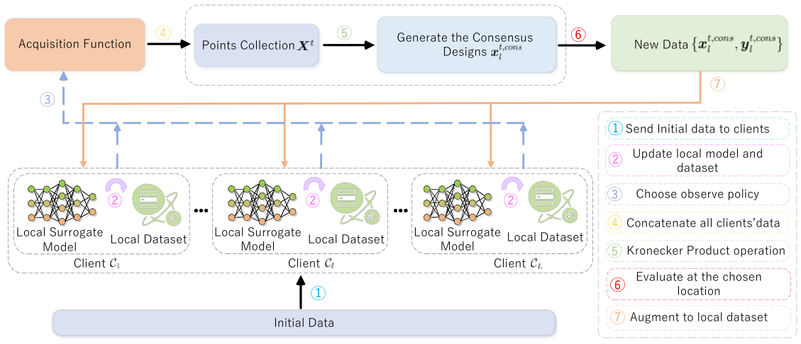
In this section, we introduce the case of multi-task collaborative BO among multiple clients based on domain expert prior knowledge. This proposed method is referred to as PMCBO. The overall framework of our PMCBO method is shown in Figure 1. The goal of PMCBO is to utilize domain expert prior knowledge to improve multi-task BO performance for multi-agent systems. Concretely, we first sample an arbitrary objective function $f_l$ at some points ${\mathit{x}}_l$, which is guided by prior knowledge. Meanwhile, data exchange occurs among different clients to further adjust the values of sampled points. In comparison to vanilla Bayesian optimization, PMCBO allows for the discovery of optimal function values in fewer optimization iterations, which effectively decreases optimization costs.

4.1. Decaying Prior-Informed Acquisition Function

We first incorporate the domain expert prior knowledge in PMCBO. Assuming the expert prior knowledge about the promising location of regions for the $l_{th}$ objective functions ${\left\{f_l\right\}}_{l=1}^L$, we depict the domain expert prior knowledge as a probability distribution concerning ${\mathit{x}}_l$, denoted as $\pi ({\mathit{x}}_l)$. Then, we guide the collection of some new points $\mathit{x}$ by using a prior probability of this distribution. The prior probability of an arbitrary objective function $f_l$ is defined as follows:

$$\begin{array}{c}\hfill {\mathrm{\Psi }}_l({\pi }_l({\mathit{x}}_l))=\mathbb{P}({\mathit{x}}_l=\underset{{\mathit{x}}_l^{\star }\in \mathcal{X}}{arg\; min}{f}_l({\mathit{x}}_l^{\star })),\end{array}$$

(6)

where ${\mathit{x}}_l^{\star }$ is the location of global optimum for the objective function $f_l$. In addition, we also define the optimal prior probability as ${\mathrm{\Psi }}_l({\pi }_l({\mathit{x}}_l^{\star }))$.

Without loss of generality, we assume that any point in the entire function space $\mathcal{X}$ could potentially be the location of the global optimum, utilizing the expert prior probability $\mathrm{\Psi }(\pi (\mathit{x}))$ to guide the sample, which aims to explore the regions with “high-quality” function values. Nevertheless, the expert brief may be inaccurate or even incorrect, which may result in multiple samplings of “low-quality” regions throughout the optimization process. To address this issue, we develop variants of the sigmoid function to attenuate the prior probability $\mathrm{\Psi }(\pi (\mathit{x}))$ during the optimization process. The purpose is to gradually reduce the dependency of the acquisition function on $\mathrm{\Psi }(\pi (\mathit{x}))$ as the optimization process evolves.

In the initial stage of optimization, the surrogate model has limited understanding of the objective function; we should rely more on the prior $\mathrm{\Psi }(\pi (\mathit{x}))$, and as the optimization progresses, trusting in the surrogate model should be emphasized rather than the prior $\mathrm{\Psi }(\pi (\mathit{x}))$. Souza et al. [39] used $\gamma ={\displaystyle \frac{n}{t}}$ to enhance the influence of the surrogate. Moreover, Hvarfner et al. [41] utilized $\gamma ={\displaystyle \frac{\beta }{t}}$ to decay the influence of the prior $\mathrm{\Psi }(\pi ({\mathit{x}}^{\star }))$. However, the aforementioned methods employ a linear approach to mitigate the influence of priors, which struggles to exhibit good performance in the distributed framework. Thus, we implement the nonlinear method inspired by the sigmoid function, setting decay factor ${\gamma }_t(\omega )=({\displaystyle \frac{1}{1+e^{\omega t}}})$, where $\omega \in {\mathbb{R}}^{+}$ is a hyperparameter that represents the confidence in $\mathrm{\Psi }(\pi (\mathit{x}))$ and t is the iteration number. At iteration t, we define the decaying prior-informed acquisition function on the basis of a given acquisition function $\alpha (\mathit{x},{\mathcal{D}}^t)$ with the expert prior probability $\mathrm{\Psi }(\pi (\mathit{x}))$ as

$$\begin{array}{cc}\hfill \alpha (\mathit{x},{\mathcal{D}}^t,\mathrm{\Psi })& :=\alpha (\mathit{x},{\mathcal{D}}^t)\mathrm{\Psi }{(\pi (\mathit{x}))}^{{\gamma }_t(\omega )},\hfill \\ \hfill & =\alpha (\mathit{x},{\mathcal{D}}^t)\mathrm{\Psi }{(\pi (\mathit{x}))}^{({\displaystyle \frac{1}{1+e^{\omega t}}})}.\hfill \end{array}$$

(7)

To further clarify the effect of $\omega$, we analyze its limiting cases. For any fixed $t>0$, we have

$$\begin{array}{cc}\hfill \underset{\omega \to \infty }{lim}\mathrm{\Psi }{(\pi (x))}^{{\gamma }_t(\omega )}& =1,\hfill \\ \hfill \underset{\omega \to 0}{lim}\mathrm{\Psi }{(\pi (x))}^{{\gamma }_t(\omega )}& =\sqrt{\mathrm{\Psi }(\pi (x))}.\hfill \end{array}$$

Therefore, a small $\omega$ retains the influence of the expert prior for a longer period, whereas a large $\omega$ rapidly removes its influence and makes the proposed acquisition function approach the corresponding vanilla acquisition function.

We acquire points $\mathit{x}$ through maximizing the prior-informed acquisition function $\alpha (\mathit{x},{\mathcal{D}}^t,\mathrm{\Psi })$. With the increase in iteration t, the exponent on the prior probability will tend toward zero, which implies that the prior tends toward uniformity. Thus, with growing t, the prior-informed acquisition function of $\alpha (\mathit{x},{\mathcal{D}}^t,\mathrm{\Psi })$ tends to converge towards $\alpha (\mathit{x},{\mathcal{D}}^t)$. Concretely, we will provide the theoretical analysis in Section 5.

4.2. Collaborative Multi-Task BO Among Multiple Clients

We currently consider the scenario within a distributed framework for the $l_{th}$ client at an arbitrary iteration t. Our goal is to facilitate information exchange among all clients to collaboratively determine the next sampling point for data collection. The works [63,64] have proposed the concept of “consensus” to facilitate collaboration and distributed experiments across all clients. In the background of the DBO framework, the consensus design enables arbitrary client ${\mathcal{C}}_l$ to exchange information with its neighbors ${\mathcal{N}}_{{\mathcal{C}}_l}$ over the network $\mathcal{G}$ and reaches an agreement on their next sampling point designs based on a consensus matrix. More specifically, we represent the process of collecting function sample points in a distributed framework as

$$\begin{array}{cc}\hfill {\mathit{x}}_l^t={[{\mathit{X}}^t]}_l& =\underset{\mathit{x}\in \mathcal{X}}{arg\; max}\alpha (\mathit{x},{\mathcal{D}}^t,\mathrm{\Psi }),\hfill \end{array}$$

(8)

$$\begin{array}{cc}\hfill {\mathit{x}}_l^{t,cons}& ={[({\mathit{W}}^t\otimes {\mathit{I}}_d){\mathit{X}}^t]}_l,\hfill \end{array}$$

(9)

where ${[·]}_k$ represents the point x of the $l_{th}$ client at iteration t and $[{\mathit{X}}^t]=[{\mathit{x}}_1^t,{\mathit{x}}_2^t,\dots ,{\mathit{x}}_L^t]$ is the collection of sampled points among all clients. $\mathit{W}$ is a consensus matrix of order L depicted as

$$\begin{array}{c}\hfill \mathit{W}=\left(\begin{array}{cccc}{\omega }_{11}& {\omega }_{12}& \cdots & {\omega }_{1L}\\ {\omega }_{21}& {\omega }_{22}& \cdots & {\omega }_{2L}\\ ⋮& ⋮& \ddots & ⋮\\ {\omega }_{L1}& {\omega }_{L2}& \cdots & {\omega }_{LL}\end{array}\right),\end{array}$$

where ${\mathit{I}}_d$ is an identity matrix with its order equal to the dimension of input $\mathit{x}$. ⊗ indicates the Kronecker Product operation; i.e., assume the dimension of $\mathit{x}$ is d, $({\mathit{W}}^t\otimes {\mathit{I}}_d)$ yields a matrix with order $dL\times dL$. In addition, the matrix $\mathit{W}$ is a symmetric, doubly stochastic matrix with positive elements, i.e., ${\sum }_l{\omega }_{lj}={\sum }_j{\omega }_{jl}=1,j,l\in \{1,\dots ,L\}$.

The procedure of the PMCBO method is depicted in Algorithm 1, which considers the original observation ${\left\{{\mathcal{D}}_l^0\right\}}_{l=1}^L$ across all clients. In each iteration, PMCBO collects candidate points $\mathit{x}$ across all clients by means of decaying the prior-informed acquisition function $\alpha (\mathit{x},{\mathcal{D}}^t,\mathrm{\Psi })$. Then, a consensus matrix is utilized to harness the collective strength among all clients. Thus, we can predict the mean $\mu (\mathit{x})$ and uncertainty $\sigma (\mathit{x})$, which are used for the next iteration of data collection. Notably, the consensus matrix describes how clients mutually influence each other. Hence, the design of the consensus matrix becomes a pivotal issue that demands our careful consideration.

Algorithm 1 PMCBO

1: Input: L number of clients with corresponding objective functions ${\left\{f_l\right\}}_{l=1}^L$, initial data ${\left\{{\mathcal{D}}_l^0\right\}}_{l=1}^L$, initial consensus matrix ${\mathit{W}}^0$, initial candidate points among all clients ${\left\{{\mathit{x}}_l^0\right\}}_{l=1}^L$ with design points concatenation $[{\mathit{X}}^0]=[{\mathit{x}}_1^0,{\mathit{x}}_2^0,\dots ,{\mathit{x}}_L^0]$, T iterations. 2: while  $t<T$  do 3:    for $l=1$  to L do 4:      All clients engage in consensus optimization. 5:      ${\mathit{x}}_l^{t,cons}={[({\mathit{W}}^t\otimes {\mathit{I}}_d){\mathit{X}}^t]}_l$ 6:      $y_l^{t,cons}=f({\mathit{x}}_l^{t,cons})+{ϵ}_l^t$ 7:      ${\mathcal{D}}_l^{t+1}={\mathcal{D}}_l^t\cup \{{\mathit{x}}_l^{t,cons},y_l^{t,cons}\}$ 8:      Fit GP Model. 9:      Select ${\mathit{x}}_l^{t+1}={arg\; max}_{\mathit{x}\in \mathcal{X}}\alpha (\mathit{x},{\mathcal{D}}^t,\mathrm{\Psi })$ 10:    end for 11: end while

4.3. Construction of Consensus Matrix

In the initial stage of the distributed framework, we assume that all clients are mutually connected. Furthermore, we design the consensus matrix by assigning the same value to all elements within this matrix. Considering its doubly stochastic property, the initial consensus matrix ${\mathit{W}}^0$ is represented as

$$\begin{array}{c}\hfill {\mathit{W}}^0=\left(\begin{array}{cccc}{\displaystyle \frac{1}{L}}& {\displaystyle \frac{1}{L}}& \cdots & {\displaystyle \frac{1}{L}}\\ ⋮& ⋮& \ddots & ⋮\\ {\displaystyle \frac{1}{L}}& {\displaystyle \frac{1}{L}}& \cdots & {\displaystyle \frac{1}{L}}\end{array}\right).\end{array}$$

Although the early information exchange can facilitate consensus optimization among multiple clients, as optimization progresses, we should pay more attention to personalized strategies for individual clients. Therefore, the design of the consensus matrix ${\mathit{W}}^t$ evolves over time, which will eventually become an identity matrix as t grows. We increase the weights by ${\displaystyle \frac{L-1}{TL}}$ for diagonal elements and decrease the weights by ${\displaystyle \frac{1}{TL}}$ for non-diagonal elements. As a result, the update of the consensus matrix is expressed as follows:

$$\begin{array}{c}\hfill {\mathit{W}}^{t+2}={\mathit{W}}^{t+1}+\left(\begin{array}{cccc}{\displaystyle \frac{L-1}{TL}}& -{\displaystyle \frac{1}{TL}}& \cdots & -{\displaystyle \frac{1}{TL}}\\ ⋮& ⋮& \ddots & ⋮\\ -{\displaystyle \frac{1}{TL}}& -{\displaystyle \frac{1}{TL}}& \cdots & {\displaystyle \frac{L-1}{TL}}\end{array}\right).\end{array}$$

(10)

In the initial phase, client l lacks sufficient observations to derive a high-quality utility on its own, so it relies more heavily on information borrowed from other clients. As its local data grows in later stages, client l will focus more on its own design problem, and finding client-specific optimal points.

Another approach is the “leader-driven matrix”, which is inspired by [42]. It adjusts the weights of W dynamically based on the “leader”, i.e., the client that observed the best improvement. Consequently, the remaining clients are guided by the leader to investigate regions with high potential for optimal solutions. At the initialization stage, two matrices, ${\mathit{W}}_1^0$ and ${\mathit{W}}_2^0$, are established with uniformly distributed weights. Matrix ${\mathit{W}}_1$ serves as a baseline reference updated via Equation (10), while matrix $W_2$ is adjusted by integrating both ${\mathit{W}}_1$ and the leader’s information. Matrix ${\mathit{W}}_1$ is introduced as an identity-directed transitional baseline, which is intended to guide Matrix ${\mathit{W}}_2$ toward increasingly client-specific weighting as the optimization proceeds.

In this case, each client obtains its information pair $\{{\mathit{x}}_l^{t,cons},y_l^{t,cons}\}$ for the corresponding objective at iteration t. Then, we collect the information pairs from all clients in this round, denoted as ${\sum }_{l=1}^L\{{\mathit{x}}_l^{t,cons},y_l^{t,cons}\}$. Thus, comparing the $\left\{y_l^{t,cons}\right\}$ across all information pairs and the corresponding client with the optimal $y_l^{t,cons}$ value (maximum or minimum) is considered as the leader client for round t. Assume client ${\mathcal{C}}_l$ is the leader at iteration t (i.e., ${\mathcal{C}}_l^{*}$), the leader client ${\mathcal{C}}_l^{*}$ can communicate with others that there is a “high-quality” region for exploration. In this case, for the leader client ${\mathcal{C}}_l^{*}$, we decrease its weights by ${\displaystyle \frac{{(L-1)}^2}{TL}}$ and update the weights of non-leader clients ${\mathcal{C}}_l$, (i.e., $l\ne l^{*}$) by ${\displaystyle \frac{1}{TL}}$. For this purpose, we modify blocks of ${\mathit{W}}^{(t+1)}$ as follows:

$$\begin{array}{c}{[{\mathit{W}}_{\mathbf{2}}^{(t)}]}_{\ne l^{(t)},l^{(t)}}={[{\mathit{W}}_{\mathbf{1}}^{(t)}]}_{\ne l^{(t)},l^{(t)}}+{\displaystyle \frac{L-1}{TL}},\\ [{\mathit{W}}_{\mathbf{2}}^{(t)}{]}_{l^{(t)},\ne l^{(t)}}={[{\mathit{W}}_{\mathbf{1}}^{(t)}]}_{l^{(t)},\ne l^{(t)}}+{\displaystyle \frac{L-1}{TL}},\\ [{\mathit{W}}_{\mathbf{2}}^{(t)}{]}_{\ne l^{(t)},\ne l^{(t)}}={[{\mathit{W}}_{\mathbf{1}}^{(t)}]}_{\ne l^{(t)},\ne l^{(t)}}-{\displaystyle \frac{1}{TL}},\\ [{\mathit{W}}_{\mathbf{2}}^{(t)}{]}_{l^{(t)},l^{(t)}}={[{\mathit{W}}_{\mathbf{1}}^{(t)}]}_{l^{(t)},l^{(t)}}-{\displaystyle \frac{{(L-1)}^2}{TL}},\end{array}$$

where ${[{\mathit{W}}_2^{(t)}]}_{\ne i,j}$ represents all elements that are in the $j_{th}$ column but not in the $i_{th}$ row of ${\mathit{W}}_2^{(t)}$ and ${[{\mathit{W}}_2^{(t)}]}_{i,j}$ denotes the element at the $i_{th}$ row and $j_{th}$ column in the matrix.

The proposed PMCBO method will continue running until the number of evaluations T reaches the allocated budget. In line nine of Algorithm 1, the points among all clients are sampled based on expert prior knowledge. Then, they progress to consensus design in line five of Algorithm 1 with interactions across all clients.

5. Theoretical Results

Despite the fact that the proposed PMCBO method is tough to analyze directly owing to the unknown structure of objective functions ${\left\{f_l\right\}}_{l=1}^L$ across all clients, we still provide a rigorous analysis for the proposed PMCBO method in this section. To this end, we combine EI [23], GP-UCB [65] acquisition functions, and the GP model to derive some theoretical insights. In addition, the general framework for the variable selection under consideration is outlined as follows: in each iteration, after selecting a set of variables based on prior knowledge, we then redistribute weights through the consensus matrix, and the corresponding observation data (i.e., the data points sampled so far among all clients) are utilized to update a GP model.

5.1. Loss Analysis for Prior-Informed Acquisition Function

Let ${\mathit{x}}_l^{\star }$ represent the optimal solution for client ${\mathcal{C}}_l$. We begin by considering the worst-case loss incurred in sampling points $\mathit{x}$ over the RKHS ball $B_R$ that a function $f_l$ of norm ${\parallel f\parallel }_{\mathcal{H}}\le B$ in the RKHS, which is defined as

$$\begin{array}{c}\hfill {\mathcal{L}}_l^t(u,{\mathcal{D}}^t,\mathcal{H}(\mathcal{X}),B)\triangleq \underset{{\parallel f\parallel }_{\mathcal{H}(\mathcal{X})}\le B}{sup}{\mathbb{E}}_f[f({\mathit{x}}_l^{in,t})-f({\mathit{x}}_l^{\star })],\end{array}$$

where $f({\mathit{x}}_l^{in,t})$ is the incumbent that is the best observed value so far in the observation set ${\mathcal{D}}^t$ up to round t and u is a strategy for choosing points $\mathit{x}$. To analyze the loss of the prior-informed acquisition function, we introduce the following assumption.

Assumption 1.

A symmetric positive definite function K is $C^{[k]}$, i.e., k times differentiable, where k is the largest integer less than $2\nu$. Moreover, the k-th order Taylor Approximation $P_k$ of K fulfills

$$\begin{array}{c}\hfill |K(\mathit{x})-P_k{(\mathit{x})|=\mathcal{O}(\parallel \mathit{x}\parallel }^{2\nu }{(-log\parallel \mathit{x}\parallel )}^{\alpha })\end{array}$$

as $\mathit{x}\to 0$ for some $\alpha \ge 0$, where α controls the decay rate of the logarithmic factor; then, the smoothness of the kernel function K can be adjusted. Furthermore, ν reins in the smoothness of kernel functions from the prior [66], where this covariance is $\lceil \nu \rceil -1$ times continuously differentiable.

Next, we present the following theoretical result for the prior-informed acquisition function.

Theorem 1.

Given the observation set ${\mathcal{D}}^t$, kernel function K_ℓ with fixed length scale ℓ, the global variation scale σ, and sampling strategy $\mathrm{\Psi }(\pi (\mathit{x}))$, then the loss ${\mathcal{L}}_l^t$ for client ${\mathcal{C}}_l$ at iteration t can be bounded as

$$\begin{array}{c}\hfill {\mathcal{L}}_l^t(E{I}_{\mathrm{\Psi }}^t,{\mathcal{D}}^t,\mathcal{H}(\mathcal{X}),B)\le C_{\mathrm{\Psi }}^t{\mathcal{L}}_l^t(E{I}_l^t,{\mathcal{D}}^t,\mathcal{H}(\mathcal{X}),B),\end{array}$$

where $C_{\mathrm{\Psi }}^t$ is a constant corresponding to prior Ψ.

As the optimization iterations t increase, the decaying factor ${\gamma }_t(\omega )$ will gradually tend to zero, which results in the constant $C_{\mathrm{\Psi }}^t$ converging to one. Thus, the prior-informed acquisition function $\alpha (\mathit{x},{\mathcal{D}}^t,\mathrm{\Psi })$ will gradually converge to the vanilla acquisition function $\alpha (\mathit{x},{\mathcal{D}}^t)$. Based on Assumption 1, we can obtain a convergence rate of ${\mathcal{L}}_l^t=\mathcal{O}(t^{-(\nu \wedge 1)/d}{(logt)}^{\alpha })$.

Proof of Theorem 1.

We first establish the bound of $E{I}_{\mathrm{\Psi }}$ to that of vanilla $EI$ (i.e., depicted in Equation (4)) regarding the loss $\mathcal{L}$ in Theorem 1. Then, we analyze the local loss ${\mathcal{L}}_l^t$ for the arbitrary objective function of client ${\mathcal{C}}_l$ at iteration t. □

Lemma 1.

Given kernel function length scale ℓ$\in {\mathbb{R}}_{+}^d$, there is a constant $C\ge 0$, and for any $h\in \mathbb{N},{\mathit{x}}_l^t\in \mathcal{X}$, the inequality concerning the posterior variance Equation (2) satisfies the following equation at most h times,

$$\begin{array}{c}\hfill {\sigma }_l^t({\mathit{x}}_l^{t+1};{\ell }_l^t)\ge C{h}^{-(\nu \wedge 1)/d}{(logh)}^{\alpha },\end{array}$$

where α is a parameter that depicted in Assumption 1, and we set

$$\alpha :=\left\{\begin{array}{cc}\alpha ,\hfill & \hfill \nu \le 1,\\ 0,\hfill & \hfill \nu >1.\end{array}\right.$$

Proof. 

We begin with displaying the posterior variance ${\sigma }^2$ (i.e., to make it easier to understand, we denote the posterior variance of client ${\mathcal{C}}_l$ at iteration t as ${[{\sigma }^2]}_l^t$) is bounded by the distance to the nearest design point. Let ${\pi }_l^t$ denote the prior with variance ${\sigma }^2=1$ and the length scale is ${\ell }_l^t$. Then for any $i\le t$, as ${\widehat{f}}_l^t(\mathit{x};{\ell }_l^t)={\mathbb{E}}_{\pi }[f_l(\mathit{x})|{\mathcal{D}}_t]$, we obtain

$$\begin{array}{cc}\hfill {[{\sigma }^2]}_l^t\left(\mathit{x};{\ell }_l^t\right)& ={\mathbb{E}}_{\pi }\left[{\left(f_l(\mathit{x})-{\widehat{f}}_l^t\left(\mathit{x};{\ell }_l^t\right)\right)}^2\mid {\mathcal{D}}_t\right]\hfill \\ \hfill & ={\mathbb{E}}_{\pi }\left[{\left(f_l(\mathit{x})-f_l\left({\mathit{x}}^i\right)\right)}^2-{\left(f_l\left({\mathit{x}}^i\right)-{\widehat{f}}_l\left(\mathit{x};{\ell }_l^t\right)\right)}^2\mid {\mathcal{D}}_t\right]\hfill \\ \hfill & \le {\mathbb{E}}_{\pi }\left[{\left(f_l(\mathit{x})-f_l\left({\mathit{x}}^i\right)\right)}^2\mid {\mathcal{D}}_t\right]\hfill \\ \hfill & =2\left(1-K_{\theta }\left(\mathit{x}-{\mathit{x}}^i\right)\right).\hfill \end{array}$$

If $\nu \le {\displaystyle \frac{1}{2}}$, based on Assumption 1, we can conclude that

$$\begin{array}{c}\hfill |K(\mathit{x})-K(0)|=\mathcal{O}(\parallel \mathit{x}{\parallel }^{2\nu }{(-log\parallel \mathit{x}\parallel )}^{2\alpha }).\end{array}$$

As $\mathit{x}\to 0$, when ${\displaystyle \frac{1}{2}}<\nu <1$, the kernel K is differential. Moreover, we can get $k(0)=1$ while K is symmetric; thus $\nabla K(0)=0$, and we can conclude that

$$\begin{array}{c}\hfill |K(\mathit{x})-K(0)|=|K(\mathit{x})-K(0)-\mathit{x}\nabla K(0)|=\mathcal{O}(\parallel \mathit{x}{\parallel }^{2\nu }{(-log\parallel \mathit{x}\parallel )}^{2\alpha }).\end{array}$$

Similarly, if $\nu >1$, then K is $C^{[2]}$, i.e., twice continuously differentiable, and thus we have

$$\begin{array}{c}\hfill |K(\mathit{x})-K(0)|=|K(\mathit{x})-K(0)-\mathit{x}\nabla K(0)|=\mathcal{O}(\parallel \mathit{x}{\parallel }^2).\end{array}$$

In conclusion, for the three scenarios involving $\nu$, we obtain

$$\begin{array}{c}\hfill |1-K(\mathit{x})|=|K(\mathit{x})-K(0)|={\mathcal{O}(\parallel \mathit{x}\parallel }^{2(\nu \wedge 1)}{(-log\parallel \mathit{x}\parallel )}^{2\alpha }),\end{array}$$

and

$$\begin{array}{c}\hfill {\sigma }_l^t({\mathit{x}}_l^{t+1};{\ell }_l^t)\le C_1^2\parallel \mathit{x}-{\mathit{x}}^i{\parallel }^{2(\nu \wedge 1)}(-log\parallel \mathit{x}-{\mathit{x}}^i{\parallel )}^{2\alpha },\end{array}$$

for a constant $C_1>0$ depending on $\mathcal{X},K$ and ℓ.

We next show that design points ${\mathit{x}}^{t+1}$ are close to a previous point ${\mathit{x}}^i$. The function space $\mathcal{X}$ is bounded, so $\mathcal{X}$ can be covered by h balls of radius $\mathcal{O}(h^{-1/d})$. Assume ${\mathit{x}}^{t+1}$ lies in a ball containing some earlier points ${\mathit{x}}^i$, then we may conclude

$$\begin{array}{c}\hfill {[{\sigma }^2]}_l^t({\mathit{x}}_l^{t+1};{\ell }_l^t)\ge C_2^2{h}^{-2(\nu \wedge 1)/d}{(logh)}^{2\alpha }\end{array}$$

for a constant $C_2>0$ depending only on $\mathcal{X}$, K and ℓ. Hence, there are at most h design points ${\mathit{x}}^{t+1}$ that can be found in the h balls, satisfying

$$\begin{array}{c}\hfill {\sigma }_l^t({\mathit{x}}_l^{t+1};{\ell }_l^t)\ge C_2{h}^{-(\nu \wedge 1)/d}{(logh)}^{\alpha }.\end{array}$$

□

We next provide bounds when objective function f lies in RKHS.

Lemma 2.

Let RKHS norm ${\parallel f\parallel }_{\mathcal{H}(\mathcal{X})}\le B$, for $\mathit{x}\in \mathcal{X},t\in \mathbb{N}$ and set improvement $I={(f(\mathit{x})-f^{in})}^{+}$ and $\sigma ={\sigma }_l^t(\mathit{x},\ell )$; we can get

$$\begin{array}{c}\hfill \tau (\mathit{x}):=\mathit{x}\mathrm{\Phi }(\mathit{x})+\varphi (\mathit{x}).\end{array}$$

(11)

Moreover, we also have

$$\begin{array}{c}\hfill max(I-B\sigma ,{\displaystyle \frac{\tau (\frac{-B}{ϵ})}{\tau (\frac{B}{ϵ})}}I)\le EI(\mathit{x};\mathrm{\Psi })\le I+(B+ϵ)\sigma .\end{array}$$

(12)

Proof. 

By the conclusion of Lemma 6 in [66], if posterior standard deviation $\sigma =0$, the estimated function value $f(\mathit{x})$ is equal to the incumbent $f^{in}$, i.e., $f(\mathit{x})$ = $f^{in}$. Therefore, from Equation (12), we obtain $EI(\mathit{x};\mathrm{\Psi })=I$. However, in real-world scenarios, due to the influence of additive Gaussian noise $ϵ$, the posterior standard deviation s is typically zero. We subsequently analyze the scenario of $s>0$, and set $m={\displaystyle \frac{(f(\mathit{x})-f^{in})}{\sigma }}$, $u={\displaystyle \frac{(y(\mathit{x})-f^{in})}{\sigma }}$. Based on Equations (8) and (9) in [66], we can get

$$\begin{array}{c}\hfill E{I}^t(\mathit{x},\mathrm{\Psi })=ϵ\sigma \tau ({\displaystyle \frac{u}{ϵ}}).\end{array}$$

By Lemma 6 of [66], we have $|u-m|\le B$. From Equation (11), the derivative of $\tau (z)$ is $\mathrm{\Phi }(z),\mathrm{\Phi }(z)\in [0,1]$, and $\tau (z)\le 1+z$ for $z\ge 0$. Hence, we obtain

$$\begin{array}{c}\hfill E{I}^t(\mathit{x},\mathrm{\Psi })\le ϵ\sigma \tau ({\displaystyle \frac{m^{+}+B}{ϵ}})\le ϵ\sigma ({\displaystyle \frac{m^{+}+B}{ϵ}}+1)=I+(B+ϵ)\sigma .\end{array}$$

The improvement $I\ge 0$; thus $EI\ge 0$, and we can easily deduce $\tau (z)\ge 0$ owing to $EI(\mathit{x})=\sigma (\mathit{x})\tau (z)\ge 0$ for all $z\in \mathbb{R}$, and $\tau (z)=z+\tau (-z)\ge z$. Thus, we have

$$\begin{array}{c}\hfill E{I}^t(\mathit{x},\mathrm{\Psi })\ge ϵ\sigma \tau ({\displaystyle \frac{m-B}{ϵ}})\ge ϵ\sigma ({\displaystyle \frac{m-B}{ϵ}})=I-B\sigma .\end{array}$$

Moreover, because $\tau$ is increasing, we get

$$\begin{array}{c}\hfill E{I}^t(\mathit{x},\mathrm{\Psi })\ge ϵ\sigma \tau ({\displaystyle \frac{-B}{ϵ}}).\end{array}$$

Combining these bounds and eliminating $\sigma$, we obtain

$$\begin{array}{c}\hfill E{I}^t(\mathit{x},\mathrm{\Psi })\ge {\displaystyle \frac{ϵ\tau (\frac{-B}{ϵ})}{B+ϵ\tau (\frac{-B}{ϵ})}}I={\displaystyle \frac{\tau (\frac{-B}{ϵ})}{\tau (\frac{B}{ϵ})}}I.\end{array}$$

□

Proof of Theorem 1.

We bound the expected improvement by the actual improvement I. Subsequently, we utilize the ${max}_{\mathit{x}\in \mathcal{X}}{\mathrm{\Psi }}^t(\mathit{x})$ to bound $E{I}_{\mathrm{\Psi }}$ for any point $\mathit{x}\in \mathcal{X}$ at iteration t.

$$\begin{array}{c}\hfill {\displaystyle \frac{E{I}^t(\mathit{x},\mathrm{\Psi })}{{max}_{\mathit{x}\in \mathcal{X}}{\mathrm{\Psi }}^t(\mathit{x})}}={\displaystyle \frac{E{I}^t(\mathit{x}){\mathrm{\Psi }}^t(\mathit{x})}{{max}_{\mathit{x}\in \mathcal{X}}{\mathrm{\Psi }}^t(\mathit{x})}}\le E{I}^t(\mathit{x})\le I^t+(B+ϵ)\sigma .\end{array}$$

For the lower bounds, we rely on the expert prior ${min}_{\mathit{x}\in \mathcal{X}}\mathrm{\Psi }(\mathit{x})$; similarly,

$$\begin{array}{c}\hfill max(I^t-B\sigma ,{\displaystyle \frac{\tau (\frac{-B}{ϵ})}{\tau (\frac{B}{ϵ})}}{I}^t)\le E{I}^t(\mathit{x})\le {\displaystyle \frac{E{I}^t(\mathit{x}){\mathrm{\Psi }}^t(\mathit{x})}{{min}_{\mathit{x}\in \mathcal{X}}{\mathrm{\Psi }}^t(\mathit{x})}}={\displaystyle \frac{E{I}_{\mathrm{\Psi }}^t(\mathit{x})}{{min}_{\mathit{x}\in \mathcal{X}}{\mathrm{\Psi }}^t(\mathit{x})}}.\end{array}$$

Consequently, $E{I}_{\mathrm{\Psi }}$ can be bounded by the actual improvement as

$$\begin{array}{c}\hfill \underset{\mathit{x}\in \mathcal{X}}{min}{\mathrm{\Psi }}^t(\mathit{x})\underset{\mathit{x}\in \mathcal{X}}{max}(I^t-B\sigma ,{\displaystyle \frac{\tau (\frac{-B}{ϵ})}{\tau (\frac{B}{ϵ})}}{I}^t)\le E{I}_{\mathrm{\Phi }}^t(\mathit{x})\le \underset{\mathit{x}\in \mathcal{X}}{max}{\mathrm{\Psi }}^t(\mathit{x})(I^t+(B+ϵ)\sigma ).\end{array}$$

With the aforementioned bounds, we consider the setting as in the proof for Theorem 2 in [66], which proves an upper bound for the $EI$ strategy under fixed parameters. If there exists a time $t_h$, $h\le t_h\le 3h$, the posterior variance will be bounded by $C{h}^{-(\nu \wedge 1)/d}{(logh)}^{\alpha }$. Furthermore, since $I\ge 0$ and ${\parallel f\parallel }_{\mathcal{H}(\mathcal{X})}\le B$, we can bound the total improvement as

$$\begin{array}{c}\hfill \sum _t{I}^t\le \sum _t(f({\mathit{x}}^{in,t})-f({\mathit{x}}^{in,t+1}))\le f(x^{in,1}-minf)\le 2{\parallel f\parallel }_{\infty }\le 2B,\end{array}$$

where $f({\mathit{x}}^{in,t})$ and $f({\mathit{x}}^{in,t+1})$ are the optimal values observed up to rounds t and $t+1$, respectively. Thus, $f({\mathit{x}}^{in,t}-f({\mathit{x}}^{in,t+1}))>2B{h}^{-1}$ at most h times. Since $f({\mathit{x}}^{in,t}-f({\mathit{x}}^{t+1})\le f({\mathit{x}}^{in,t}-f({\mathit{x}}^{in,t+1}))$, we also have $f({\mathit{x}}^{in,t}-f({\mathit{x}}^{t+1})>2B{h}^{-1}$ at most h times. Therefore, the posterior variance ${[{\sigma }^2]}^{t_h}$ and the expected improvement $I^{t_h}$ are bounded at time $t_h$. Considering an arbitrary iteration t, $3h\le t\le 3(h+1)$, we use the bounds on $E{I}_{\mathrm{\Psi }},{\sigma }^{t_h}$, and $I^{t_h}$ to obtain the bounds on the $E{I}_{\mathrm{\Psi }}$ loss as follows:

$$\begin{array}{cc}\hfill & {\mathcal{L}}_l^t(E{I}_{\mathrm{\Psi }}^t,{\mathcal{D}}^t,\mathcal{H}(\mathcal{X}),B)=f({\mathit{x}}^{in,t})-minf\hfill \\ \hfill & \le f({\mathit{x}}^{in,t_h})-minf\le {\displaystyle \frac{E{I}_{\mathrm{\Psi }}^{t_h}({\mathit{x}}^{in})}{{min}_{x\in \mathcal{X}}\mathrm{\Psi }(\mathit{x})}}{\displaystyle \frac{\tau (\frac{B}{ϵ})}{\tau (\frac{-B}{ϵ})}}\hfill \\ \hfill & \le {\displaystyle \frac{E{I}_{\mathrm{\Psi }}^{t_h}({\mathit{x}}^{t+1})}{{min}_{\mathit{x}\in \mathcal{X}}\mathrm{\Psi }(\mathit{x})}}{\displaystyle \frac{\tau (\frac{B}{ϵ})}{\tau (\frac{-B}{ϵ})}}\le {\displaystyle \frac{{max}_{\mathit{x}\in \mathcal{X}}\mathrm{\Psi }(\mathit{x})}{{min}_{\mathit{x}\in \mathcal{X}}\mathrm{\Psi }(\mathit{x})}}{\displaystyle \frac{\tau (\frac{B}{ϵ})}{\tau (\frac{-B}{ϵ})}}(I^{t_h}+(B+ϵ){\sigma }^{t_h})\hfill \\ \hfill & \le \left({\displaystyle \frac{{max}_{\mathit{x}\in \mathcal{X}}\mathrm{\Psi }(\mathit{x})}{{min}_{\mathit{x}\in \mathcal{X}}\mathrm{\Psi }(\mathit{x})}}\right){\displaystyle \frac{\tau (\frac{B}{ϵ})}{\tau (\frac{-B}{ϵ})}}(2B{h}^{-1}+(B+ϵ)C{h}^{-(\nu \wedge 1)/d}{(logh)}^{\alpha })\hfill \\ \hfill & \le {\left({\displaystyle \frac{{max}_{\mathit{x}\in \mathcal{X}}\mathrm{\Psi }(\mathit{x})}{{min}_{\mathit{x}\in \mathcal{X}}\mathrm{\Psi }(\mathit{x})}}\right)}^{{\gamma }_t}{\displaystyle \frac{\tau (\frac{B}{ϵ})}{\tau (\frac{-B}{ϵ})}}(2B{h}^{-1}+(B+ϵ)C{h}^{-(\nu \wedge 1)/d}{(logh)}^{\alpha }).\hfill \end{array}$$

Evidently, the inequality factor ${\left({\displaystyle \frac{{max}_{\mathit{x}\in \mathcal{X}}\mathrm{\Psi }(\mathit{x})}{{min}_{\mathit{x}\in \mathcal{X}}\mathrm{\Psi }(\mathit{x})}}\right)}^{{\gamma }_t}$ is larger than the bound on ${\mathcal{L}}^t(E{I}^t,{\mathcal{D}}^t,\mathcal{H}(\mathcal{X}),B)$. Therefore, this bound is uniform in f with ${\parallel f\parallel }_{\mathcal{H}}(\mathcal{X})\le B$, and the terms ${\gamma }_t$ gradually approach zero as t increases. Combing the all above Lemmas 1 and 2 and Assumption 1, we can get the converge rate of the loss for client ${\mathcal{C}}_l$ as

$$\begin{array}{c}\hfill {\mathcal{L}}_l^t(EI({\mathrm{\Psi }}^{\star }),{\mathcal{D}}^t,\mathcal{H}(\mathcal{X}),B)=\mathcal{O}(t^{-(\nu \wedge 1)/d}{(logt)}^{\alpha }).\end{array}$$

□

5.2. The Regret Bound of PMCBO

For an arbitrary client ${\mathcal{C}}_l$, we analyze the instant regret $r_l^t=f_l({\mathit{x}}_l^{\star })-f_l({\mathit{x}}_l^{t,cons})$ for one round and the cumulative regret $R_l^T={\sum }_{t=1}^T(f_l({\mathit{x}}_l^{\star })-f({\mathit{x}}_l^{t,cons}))$ over the entire optimization process, i.e., the regret denotes the gap between the optimum of the function values and the values at selected points $\mathit{x}$. Our goal is to achieve the “no regret” property. Thus, we may derive an upper bound on instant regret in terms of cumulative regret: $r_l^t\le R_l^T/T$ as $\underset{T\to \infty }{lim}{R}_l^T/T=0$. Let $\mathcal{X}\subset {[0,r]}^d$ be convex and compact, where $d\in \mathbb{N},r>0$. All functions $f_l$ of client ${\mathcal{C}}_l$ for all $l\in L$ satisfy the following assumption.

Assumption 2.

The function $f_l$ is a sample path from the Gaussian process. For some constants $a,b\ge 0$, considering a Lipschitz constant $\widehat{L}\ge 0$, the partial derivatives of objective function f fulfill the condition that

$$\begin{array}{c}\hfill \mathbb{P}(\forall j,\forall \mathit{x}\in \mathcal{X},\underset{\mathit{x}\in \mathcal{X}}{sup}\left|{\displaystyle \frac{\partial f_l}{\partial {\mathit{x}}_j}}\right|<{\tilde{\alpha }}_l\widehat{L})\ge 1-a{e}^{-{({\displaystyle \frac{\widehat{L}}{b}})}^2},\forall t\ge 1,\end{array}$$

where ${\tilde{\alpha }}_l$ characterizes the importance of the $l_{th}$ variable ${\mathit{x}}_l$, the larger ${\tilde{\alpha }}_l$ represents the greater essentiality of ${\mathit{x}}_l$ on the function $f_l$, and $j=1,\dots ,d$ is the dimension of ${\mathit{x}}_l$.

Assumption 2 indicates that the probability is higher than $1-a{e}^{-{({\displaystyle \frac{\widehat{L}}{b}})}^2}$. Hence, we conclude that

$$\begin{array}{c}\hfill \forall \mathit{x}\in D,|f(\mathit{x})-f({\mathit{x}}^{\prime })|\le \widehat{L}{\parallel \mathit{x}-{\mathit{x}}^{\prime }\parallel }_1.\end{array}$$

Now, we establish the regret bound for the PMCBO method as follows.

Theorem 2.

Assume all objective functions of clients are homogeneous (i.e., $f_1=f_2=\cdots =f_L$), and suppose ${\left\{f_l\right\}}_{l=1}^L$ satisfy Assumption 2, given any doubly stochastic matrix ${\mathit{W}}^t$ with all positive elements, for $\delta \in (0,1)$ and ${\beta }_t=2log({\displaystyle \frac{t^{2}2{\pi }^2}{3\delta }})+2dlog(t^{2}dbr\sqrt{log({\displaystyle \frac{4da}{\delta }})})$. Executing GP-UCB with ${\beta }_t$ for all objective functions ${\left\{f_l\right\}}_{l=1}^L$ of a GP that is characterized by a zero-mean function and a covariance function K, we obtain the regret bound of client ${\mathcal{C}}_l$ as $\mathcal{O}(\sqrt{dT{\gamma }_T})$ with high probability, i.e.,

$$\begin{array}{c}\hfill \mathbb{P}(R_l^T\le \sqrt{{\tilde{C}}_{1}T{\beta }_T{\gamma }_T}+2{\tilde{\alpha }}_{max}+{\displaystyle \sum _{t=1}^T}\sum _{i\in \left|\mathcal{X}\right|\setminus |{\mathcal{X}}_t|}{\tilde{\alpha }}_i^{\star }\widehat{L}r,\forall T\ge 1)\ge 1-\delta ,\end{array}$$

where r is the maximum coordinate discrepancy and ${\tilde{\alpha }}_i^{\star }$ is the optimal (maximum or minimum) value of ${\tilde{\alpha }}_i$. ${\gamma }_T$ is the maximum information gain after T iterations, i.e.,

$$\begin{array}{c}\hfill {\gamma }_T:=\underset{\mathcal{A}\subset \mathcal{X}:\left|\mathcal{A}\right|=T}{max}\mathbf{I}(y_{\mathcal{A}};f_{\mathcal{A}}).\end{array}$$

The regret bound of one iteration in our PMCBO method is determined by three key factors: fitting the Gaussian process surrogate model, optimizing the acquisition function, and assessing the sampled point. Furthermore, we use the squared exponential kernel, and the average cumulative regret bound of a fitting GP model at iteration t across all clients is $\mathcal{O}(\sqrt{T}{(logT)}^{{\displaystyle \frac{d+1}{2}}})$, which is better than the regret bound of CBOC [42]. Moreover, Theorem 2 demonstrates that, with a high probability drawn from GP samples, the cumulative regret remains bounded by the maximum information gain, establishing a link between GP optimization and experimental design.

Proof of Theorem 2.

We next analyze the upper bound on the cumulative regret $R_l^T={\sum }_{t=1}^T(f_l({\mathit{x}}^{\star })-f({\mathit{x}}_l^{t,cons}))$ across all clients in the DBO framework of Theorem 2. Let us begin with the analysis by the instantaneous regret $r_l^t=f_l({\mathit{x}}^{\star })-f_l({\mathit{x}}_l^{t,cons})$. Note that $R_l^T={\sum }_{t=1}^T{r}_l^t$, and let ${\mu }_{t-1}(·)$ and ${\sigma }_{t-1}^2(·)$ denote the posterior mean and variance after running $t-1$ iterations. Utilizing the $f_l({\mathit{x}}_l^{t,cons})$ denotes the consensus sampled point at iteration t for client ${\mathcal{C}}_l$. For the sake of brevity, we drop l in some symbols, such as ${\mu }_t,{\sigma }_{t-1},{\beta }_t$, and so on. □

Lemma 3.

$\forall \delta \in (0,1)$, $\forall t\ge 1$, let ${\beta }_t=2log({\pi }_t/\delta )$, where ${\sum }_{t\ge 1}{\pi }_t^{-1}=1$, ${\pi }_t>0$. Then, we know that

$$\begin{array}{c}\hfill |f_l({\mathit{x}}_l^{t,cons})-{\mu }_{t-1}({\mathit{x}}_l^{t,cons})|\le {\beta }_t^{1/2}{\sigma }_{t-1}({\mathit{x}}_l^{t,cons})\end{array}$$

holds with probability at least $1-\delta$, where ${\mathit{x}}_l^{t,cons}$ is the consensus obtained points at iteration t.

Proof. 

Considering $t\ge 1$ and ${\mathit{x}}_l^{t,cons}\in \mathcal{X}$. Conditioned on ${\mathit{y}}_{t-1}=(y_1,y_2,\dots ,y_{t-1})$, $\{{\mathit{x}}_1,{\mathit{x}}_2,\dots ,{\mathit{x}}_{t-1}\}$ are deterministic, $f_l({\mathit{x}}_l^{t,cons}\sim \mathcal{N}({\mu }_{t-1}({\mathit{x}}_l^{t,cons}),{\sigma }_{t-1}^2({\mathit{x}}_l^{t,cons})))$, and we set $z={\displaystyle \frac{f_l({\mathit{x}}_l^{t,cons})-{\mu }_{t-1}({\mathit{x}}_l^{t,cons})}{{\sigma }_{t-1}({\mathit{x}}_l^{t,cons})}}$. Thus, we have

$$\begin{array}{cc}\hfill & \mathbb{P}(|f_l({\mathit{x}}_l^{t,cons})-{\mu }_{t-1}(x_l^{t,cons})|>{\beta }_t^{1/2}{\sigma }_{t-1}({\mathit{x}}_l^{t,cons}))\hfill \\ \hfill & =\mathbb{P}(|z|>{\beta }_t^{{\displaystyle \frac{1}{2}}})=2{\int }_{{\beta }^{{\displaystyle \frac{1}{2}}}}^{\infty }{(2\pi )}^{-{\displaystyle \frac{1}{2}}}{e}^{-{\displaystyle \frac{z^2}{2}}}dz\hfill \\ \hfill & =2e^{-{\displaystyle \frac{{\beta }_t}{2}}}{\int }_{{\beta }^{{\displaystyle \frac{1}{2}}}}^{\infty }{(2\pi )}^{-{\displaystyle \frac{1}{2}}}{e}^{-{\displaystyle \frac{{(z-{\beta }_t^{\frac{1}{2}})}^2}{2}}-{\beta }_t^{{\displaystyle \frac{1}{2}}}(z-{\beta }_t^{{\displaystyle \frac{1}{2}}})}dz\hfill \\ \hfill & \le 2e^{-{\displaystyle \frac{{\beta }_t}{2}}}\mathbb{P}(z>0)\le e^{-{\displaystyle \frac{{\beta }_t}{2}}}={\displaystyle \frac{\delta }{{\pi }_t}}.\hfill \end{array}$$

Utilizing the union bound for all $t\in \mathbb{N}$, we can conclude

$$\begin{array}{c}\hfill P\left(\forall t\ge 1|f_l({\mathit{x}}_l^{t,cons})-{\mu }_{t-1}({\mathit{x}}_l^{t,cons})|\le {\beta }_t^{1/2}{\sigma }_{t-1}({\mathit{x}}_l^{t,cons})\right)\ge 1-\sum _{t\ge 1}{\displaystyle \frac{\delta }{{\pi }_t}}=1-\delta ,\end{array}$$

where ${\sum }_{t\ge 1}{\pi }_t^{-1}$ = 1. □

Next we aim to analyze the confidence bound on ${\mathit{x}}^{\star }$, utilizing a set of discretizations ${\mathcal{X}}_t\subset \mathcal{X}$, where ${\mathcal{X}}_t$ will be used at iteration t in the analysis. Lemma 4 gives a confidence bound on f for any discretized point $\mathit{x}\in {\mathcal{X}}_t$.

Lemma 4.

$\forall \delta \in (0,1)$, $\forall t\ge 1$, let ${\beta }_t=2log(|{\mathcal{X}}_t|{\pi }_t/\delta )$, where ${\sum }_{t\ge 1}{\pi }_t^{-1}=1$, ${\pi }_t>0$. Then $\forall {\mathit{x}}_l^{t,cons}\in {\mathcal{X}}_t$, and we have

$$\begin{array}{c}\hfill |f_l({\mathit{x}}_l^{t,cons})-{\mu }_{t-1}({\mathit{x}}_l^{t,cons})| \le {\beta }_t^{1/2}{\sigma }_{t-1}({\mathit{x}}_l^{t,cons})\forall {\mathit{x}}_l^{t,cons}\in {\mathcal{X}}_t,\forall t\ge 1,\end{array}$$

which holds with probability at least $1-\delta$.

Proof. 

Similar to Lemma 3, we can obtain

$$\begin{array}{c}\hfill \mathbb{P}\left(\forall t\ge 1:|f_l({\mathit{x}}_l^{t,cons})-{\mu }_{t-1}({\mathit{x}}_l^{t,cons})|>{\beta }_t^{1/2}{\sigma }_{t-1}({\mathit{x}}_l^{t,cons})\right)\le exp\left(-{\displaystyle \frac{{\beta }_t}{2}}\right)={\displaystyle \frac{\delta }{|{\mathcal{X}}_t|{\pi }_t}}.\end{array}$$

Utilizing the union bound for all $t\in \mathbb{N}$ and ${\mathit{x}}_l^{t,cons}\in {\mathcal{X}}_t$, we conclude

$$\begin{array}{c}\hfill P\left(\forall t\ge 1,:|f_l({\mathit{x}}_l^{t,cons})-{\mu }_{t-1}({\mathit{x}}_l^{t,cons})|\le {\beta }_t^{1/2}{\sigma }_{t-1}({\mathit{x}}_l^{t,cons})\right)\ge 1-\sum _{t\ge 1}\sum _{{\mathit{x}}_l^{t,cons}\in {\mathcal{X}}_t}{\displaystyle \frac{\delta }{|{\mathcal{X}}_t|{\pi }_t}}=1-\delta .\end{array}$$

Thus, we have completed the proof of Lemma 4. □

After this, by Assumption 2 and the union bound, we have

$$\begin{array}{c}\hfill P(\forall j,\forall \mathit{x}\in \mathcal{X}\underset{\mathit{x}\in \mathcal{X}}{sup}|{\displaystyle \frac{\partial f_l}{\partial {\mathit{x}}_j}}|<{\tilde{\alpha }}_i\widehat{L})\ge 1-da{e}^{-{({\displaystyle \frac{\widehat{L}}{b}})}^2},\forall t\ge 1,\end{array}$$

which indicates that the probability is higher than $1-a{e}^{-{({\displaystyle \frac{\widehat{L}}{b}})}^2}$. Hence, we conclude that

$$\begin{array}{c}\hfill \forall \mathit{x}\in \mathcal{X},|f(\mathit{x}-f({\mathit{x}}^{\prime })|\le \widehat{L}\parallel \mathit{x}-{\mathit{x}}^{\prime }{\parallel }_1.\end{array}$$

Moving forward, we obtain the confidence of ${\mathit{x}}^{\star }$ as follows. Let us begin by selecting a discretization ${\mathcal{X}}_t$ with a size of ${({\tilde{\tau }}_t)}^d$, so that for every $\mathit{x}\in \mathcal{X}$,

$$\begin{array}{c}\hfill {\parallel \mathit{x}-[\mathit{x}]}_t{\parallel }_1\le {\displaystyle \frac{\widehat{r}d}{{\tilde{\tau }}_t}},\end{array}$$

where ${[\mathit{x}]}_t$ denotes the closest point in ${\mathcal{X}}_t$ to $\mathit{x}$, $\widehat{r}\sim \mathcal{N}(0,1)$. A sufficient discretization has each coordinate with ${\tilde{\tau }}_t$ uniformly spaced points.

Subsequently, we proceed to analyze the upper bound $f_l({\mathit{x}}_l^{t,cons})$ based on Assumption 1 and Lemma 3, where ${\mathit{x}}_l^{t,cons}\in {\mathcal{X}}_t$. We first provide the confidence bound in the following Lemmas.

Lemma 5.

$\forall \delta \in (0,1)$, $\forall t\ge 1$, let ${\beta }_t=2log(2{\pi }_t/\delta )+4dlog(dtbr\sqrt{log(2da/\delta )})$, where ${\sum }_{t\ge 1}{\pi }_t^{-1}=1$. Set ${\tilde{\tau }}_t=d{t}^{2}br\sqrt{log(2da/\delta )}$ and $\widehat{L}=b\sqrt{log2da/\delta }$. Let ${[{\mathit{x}}_l^{cons,\star }]}_t$ denote the point closest to ${\mathit{x}}_l^{\star }$ in ${\mathcal{X}}_t$. Then, we know that

$$\begin{array}{c}\hfill |f_l({\mathit{x}}^{\star })-{\mu }_{t-1}({[{\mathit{x}}_l^{cons,\star }]}_t)|\le {\beta }_t^{{\displaystyle \frac{1}{2}}}{\sigma }_{t-1}({[{\mathit{x}}_l^{cons,\star }]}_t)+{\displaystyle \frac{{\tilde{\alpha }}_{max}}{t^2}}+\sum _{i\in \left|\mathcal{X}\right|\setminus |{\mathcal{X}}_t|}{\tilde{\alpha }}_i^{\star }\widehat{L}r\end{array}$$

holds with probability at least $1-\delta$, where ${\tilde{\alpha }}_i^{\star }$ is the optimal (maximum or minimum) value of ${\tilde{\alpha }}_i$ and ${\tilde{\alpha }}_{max}={max}_{i\in \left|\mathcal{X}\right|}{\tilde{\alpha }}_t^{\star }$.

Proof. 

By Assumption 1 with $\widehat{L}=b\sqrt{log2da/\delta }$, $\forall \mathit{y},\mathit{x}\in \mathcal{X}$, we have that with probability at least $1-da{e}^{-{(\widehat{L}/b)}^2}=1-{\displaystyle \frac{\delta }{2}}$,

$$\begin{array}{cc}\hfill |f(\mathit{x})-f(\mathit{y})|& \le {\displaystyle \sum _{i=1}^d}{\tilde{\alpha }}_i^{\star }\widehat{L}|{\mathit{x}}_i-{\mathit{y}}_i|\hfill \\ \hfill & \le \sum _{i\in |{\mathcal{X}}_t|}{\tilde{\alpha }}_i^{*}\widehat{L}|{\mathit{x}}_i-{\mathit{y}}_i|+\sum _{i\in \left|\mathcal{X}\right|\setminus |{\mathcal{X}}_t|}{\tilde{\alpha }}_i^{\star }\widehat{L}r\hfill \\ \hfill & \le {\tilde{\alpha }}_{max}\widehat{L}{\parallel {\mathit{x}}_i-{\mathit{y}}_i\parallel }_1+\sum _{i\in \left|\mathcal{X}\right|\setminus |{\mathcal{X}}_t|}{\tilde{\alpha }}_i^{\star }\widehat{L}r.\hfill \end{array}$$

Thus, the following relation holds with probability at least $1-{\displaystyle \frac{\delta }{2}}$,

$$\begin{array}{c}\hfill |f_l({\mathit{x}}^{\star })-f({[{\mathit{x}}_l^{cons,\star }]}_t)|\le {\tilde{\alpha }}_{max}\widehat{L}{\parallel {\mathit{x}}^{\star }-{[{\mathit{x}}_l^{cons,\star }]}_t\parallel }_1+\sum _{i\in |\mathcal{X}|\setminus |{\mathcal{X}}_t|}{\tilde{\alpha }}_i^{\star }\widehat{L}r.\end{array}$$

Using Lemma 4 and setting ${\beta }_t=2log(2{(\tilde{\tau })}^d{\pi }_t/\delta )=2log(2|{\mathcal{X}}_t|{\pi }_t/\delta )$, we can establish that the probability is at least $1-\delta /2$

$$\begin{array}{c}\hfill |f({[{\mathit{x}}_l^{cons,\star }]}_t)-{\mu }_{t-1}({[{\mathit{x}}_l^{cons,\star }]}_t)|\le {\beta }_t^{{\displaystyle \frac{1}{2}}}{\sigma }_{t-1}({[{\mathit{x}}_l^{cons,*}]}_t).\end{array}$$

Subsequently, in consideration of

$$\begin{array}{cc}\hfill |f_l({\mathit{x}}^{\star })-{\mu }_{t-1}({[{\mathit{x}}_l^{cons,\star }]}_t)|& =|f_l({\mathit{x}}^{\star })-f({[{\mathit{x}}_l^{cons,\star }]}_t)+f({[{\mathit{x}}_l^{cons,\star }]}_t)-{\mu }_{t-1}({[{\mathit{x}}_l^{cons,\star }]}_t)|\hfill \\ \hfill & \le |f_l({\mathit{x}}^{\star })-f({[{\mathit{x}}_l^{cons,\star }]}_t)|+|f({[{\mathit{x}}_l^{cons,\star }]}_t)-{\mu }_{t-1}({[{\mathit{x}}_l^{cons,\star }]}_t)|.\hfill \end{array}$$

Hence, we conclude that

$$\begin{array}{cc}\hfill |f_l({\mathit{x}}^{\star })-{\mu }_{t-1}({[{\mathit{x}}_l^{cons,\star }]}_t)|& \le {\tilde{\alpha }}_{max}\widehat{L}{\parallel {\mathit{x}}^{\star }-{[{\mathit{x}}_l^{cons,\star }]}_t\parallel }_1+\sum _{i\in \left|\mathcal{X}\right|\setminus |{\mathcal{X}}_t|}{\tilde{\alpha }}_i^{\star }\widehat{L}r+{\beta }_t^{{\displaystyle \frac{1}{2}}}{\sigma }_{t-1}({[{\mathit{x}}_l^{cons,\star }]}_t)\hfill \\ \hfill & \le {\tilde{\alpha }}_{max}\widehat{L}{\displaystyle \frac{d\widehat{r}}{\widetilde{{\tau }_t}}}+\sum _{i\in \left|\mathcal{X}\right|\setminus |{\mathcal{X}}_t|}{\tilde{\alpha }}_i^{\star }\widehat{L}r+{\beta }_t^{{\displaystyle \frac{1}{2}}}{\sigma }_{t-1}({[{\mathit{x}}_l^{cons,\star }]}_t)\hfill \\ \hfill & \le {\tilde{\alpha }}_{max}{\displaystyle \frac{1}{t^2}}+\sum _{i\in \left|\mathcal{X}\right|\setminus |{\mathcal{X}}_t|}{\tilde{\alpha }}_i^{\star }\widehat{L}r+{\beta }_t^{{\displaystyle \frac{1}{2}}}{\sigma }_{t-1}({[{\mathit{x}}_l^{cons,\star }]}_t).\hfill \end{array}$$

Here, we choose ${\tilde{\tau }}_t=d{t}^{2}br\sqrt{log(2da/\delta )}$ and apply $|{\mathcal{X}}_t| = {(d{t}^{2}br\sqrt{log(2da/\delta )})}^d$, and utilizing ${\displaystyle \frac{\delta }{2}}$ in Lemma 4, we can achieve the confidence bound to ${[{\mathit{x}}_l^{cons,\star }]}_t$ to obtain the result with the probability at least $1-\delta$. □

Now, combining with the Lemmas 3–5, we can derive an upper bound on the instantaneous regret $r_l^t$. Thus, we are currently ready to prove the upper bound on the cumulative regret $R_l^T$ in Theorem 2.

Lemma 6.

$\forall \delta \in (0,1)$, $\forall t\ge 1$ and set ${\beta }_t=2log(4{\pi }_t/\delta )+4dlog(dtbr\sqrt{log(4da/\delta )})$, where ${\sum }_{t\ge 1}{\pi }_t^{-1}=1,{\pi }_t>0$. Then, with probability greater than $1-\delta$, for all $t\in \mathbb{N}$, the regret is bounded as follows:

$$\begin{array}{c}\hfill r_l^t\le 2{\beta }_t^{{\displaystyle \frac{1}{2}}}{\sigma }_{t-1}({\mathit{x}}_l^{t,cons})+{\displaystyle \frac{{\tilde{\alpha }}_{max}}{t^2}}+\sum _{i\in \left|\mathcal{X}\right|\setminus |{\mathcal{X}}_t|}{\tilde{\alpha }}_i^{\star }\widehat{L}r.\end{array}$$

Proof. 

For all $t\ge 1$, we have

$$\begin{array}{c}\hfill r_l^t=f({\mathit{x}}^{\star })-f({\mathit{x}}_l^{t,cons}).\end{array}$$

By Lemma 5 with ${\beta }_t=2log(4{\pi }_t/\delta )+4dlog(dtbr\sqrt{log(4da/\delta )})$ and $\widehat{L}=b\sqrt{log(4da/\delta )}$, where ${\sum }_{t\ge 1}{\pi }_t^{-1}=1,{\pi }_t>0$. Set ${\tilde{\tau }}_t=d{t}^{2}br\sqrt{log(4da/\delta )}$, then,

$$\begin{array}{c}\hfill f({\mathit{x}}^{*})\le {\mu }_{t-1}({[{\mathit{x}}_l^{cons,\star }]}_t)+{\beta }_t^{{\displaystyle \frac{1}{2}}}({[x_l^{cons,\star }]}_t)+{\displaystyle \frac{{\tilde{\alpha }}_{max}}{t^2}}+\sum _{i\in \left|\mathcal{X}\right|\setminus |{\mathcal{X}}_t|}{\tilde{\alpha }}_i^{\star }\widehat{L}r\end{array}$$

holds with probability at least $1-{\displaystyle \frac{\delta }{2}}$.

Subsequently, by Lemma 3 with ${\beta }_t=2log(4{\pi }_t/\delta )+2dlog(d{t}^{2}b\widehat{r}\sqrt{log(4da/\delta )})$, we have that

$$\begin{array}{c}\hfill f({\mathit{x}}_l^{t,cons})\ge {\mu }_{t-1}({\mathit{x}}_l^{t,cons})-{\beta }_t^{{\displaystyle \frac{1}{2}}}\sigma ({\mathit{x}}_l^{t,cons})\end{array}$$

holds the probability at least $1-{\displaystyle \frac{\delta }{4}}$. Therefore, the instantaneous regret $r_l^t$ is bounded as follows:

$$\begin{array}{cc}\hfill r_l^t& \le {\mu }_{t-1}({[{\mathit{x}}_l^{cons,\star }]}_t)+{\beta }_t^{{\displaystyle \frac{1}{2}}}({[{\mathit{x}}_l^{cons,\star }]}_t)+{\displaystyle \frac{{\tilde{\alpha }}_{max}}{t^2}}+\sum _{i\in \left|\mathcal{X}\right|\setminus |{\mathcal{X}}_t|}{\tilde{\alpha }}_i^{\star }\widehat{L}r-{\mu }_{t-1}({\mathit{x}}_l^{t,cons})+{\beta }_t^{{\displaystyle \frac{1}{2}}}\sigma ({\mathit{x}}_l^{t,cons})\hfill \\ \hfill & \le {\mu }_{t-1}({\mathit{x}}_l^{t,cons})+{\beta }_t^{{\displaystyle \frac{1}{2}}}({\mathit{x}}_l^{t,cons})+{\displaystyle \frac{{\tilde{\alpha }}_{max}}{t^2}}+\sum _{i\in \left|\mathcal{X}\right|\setminus |{\mathcal{X}}_t|}{\tilde{\alpha }}_i^{\star }\widehat{L}r-{\mu }_{t-1}({\mathit{x}}_l^{t,cons})+{\beta }_t^{{\displaystyle \frac{1}{2}}}\sigma ({\mathit{x}}_l^{t,cons})\hfill \\ \hfill & =2{\beta }_t^{{\displaystyle \frac{1}{2}}}{\sigma }_{t-1}({\mathit{x}}_l^{t,cons})+{\displaystyle \frac{{\tilde{\alpha }}_{max}}{t^2}}+\sum _{i\in \left|\mathcal{X}\right|\setminus |{\mathcal{X}}_t|}{\tilde{\alpha }}_i^{\star }\widehat{L}r,\hfill \end{array}$$

where the second inequality is established because ${\mathit{x}}_l^{t,cons}$ is generated by GP-UCB. Then, we have that ${\mu }_{t-1}({[{\mathit{x}}_l^{cons,\star }]}_t)+{\beta }_t^{{\displaystyle \frac{1}{2}}}({[{\mathit{x}}_l^{cons,\star }]}_t)\le {\mu }_{t-1}({\mathit{x}}_l^{t,cons})+{\beta }_t^{{\displaystyle \frac{1}{2}}}({\mathit{x}}_l^{t,cons})$. Therefore, we complete the proof. □

Next, we combine the information gain to bound the regret.

Lemma 7.

The information gain for the points selected can be expressed in terms of the predictive variance for all functions ${\left\{f_l\right\}}_{k=1}^K$ across all clients. If $f_l^t=f_l({\mathit{x}}^t)\in {\mathbb{R}}^T$:

$$\begin{array}{c}\hfill \mathbf{I}(y_T;f_T)={\displaystyle \frac{1}{2}}{\displaystyle \sum _{t=1}^T}log(1+{\sigma }^{-2}{\sigma }_{t-1}^2({\mathit{x}}^t)).\end{array}$$

Proof. 

Recall that $\mathbf{I}(y_T;f_T)=H(y_T)-{\displaystyle \frac{1}{2}}log\left|2\pi e{\sigma }^2\mathbf{I}\right|$. Now, $H(y_T)=H(y_{T-1})+H(y_T|y_{T-1})=H(y_{T-1})+log(2\pi e({\sigma }^2+{\sigma }_{t-1}^2({\mathit{x}}_T)))/2$. Here, we use that ${\mathit{x}}_1,\dots ,{\mathit{x}}_T$ are deterministic conditioned on $y_{T-1}$, and that the conditioned variance ${\sigma }_{T-1}({\mathit{x}}_T)$ does not depend on $y_{T-1}$. □

Now, we are ready to complete the proof of Theorem 2.

Proof of Theorem 2.

By summing up $r_l^t$ from $t=1$ to T, we have derived the cumulative regret $R_l^T$ for client ${\mathcal{C}}_l$ with probability at least $1-\delta$ that, $\forall T\ge 1$,

$$\begin{array}{cc}\hfill R_l^T& ={\displaystyle \sum _{t=1}^T}{r}_l^t\le {\displaystyle \sum _{t=1}^T}2{\beta }_t^{{\displaystyle \frac{1}{2}}}{\sigma }_{t-1}({\mathit{x}}_l^{t,cons})+{\displaystyle \sum _{t=1}^T}{\displaystyle \frac{{\tilde{\alpha }}_{max}}{t^2}}+{\displaystyle \sum _{t=1}^T}\sum _{i\in \left|\mathcal{X}\right|\setminus |{\mathcal{X}}_t|}{\tilde{\alpha }}_i^{\star }\widehat{L}r\hfill \\ \hfill & \le {\displaystyle \sum _{t=1}^T}2{\beta }_t^{{\displaystyle \frac{1}{2}}}{\sigma }_{t-1}({\mathit{x}}_l^{t,cons})+2{\tilde{\alpha }}_{max}+{\displaystyle \sum _{t=1}^T}\sum _{i\in \left|\mathcal{X}\right|\setminus |{\mathcal{X}}_t|}{\tilde{\alpha }}_i^{\star }\widehat{L}r,\hfill \end{array}$$

where the second inequality holds by ${\sum }_{t=1}^T{\displaystyle \frac{1}{t^2}}\le {\displaystyle \frac{{\pi }^2}{6}}\le 2$. Furthermore, let ${\tilde{C}}_1=8/log(1+{\sigma }^{-2})$. By Lemma 5.4 in [25], we have ${\sum }_{t=1}^{T}2{\beta }_t^{{\displaystyle \frac{1}{2}}}{\sigma }_{t-1}({\mathit{x}}_l^{t,cons})\le \sqrt{{\tilde{C}}_{1}T{\beta }_T{\sum }_{t=1}^{T}log(1+{\sigma }^{-2}{\sigma }_{t-1}^2({\mathit{x}}_l^{t,cons}))/2}\le \sqrt{{\tilde{C}}_{1}T{\beta }_T{\gamma }_T}$. Finally, we apply this equation to the above inequality. The cumulative regret is represented as follows,

$$\begin{array}{c}\hfill R_l^T\le \sqrt{{\tilde{C}}_{1}T{\beta }_T{\gamma }_T}+2{\tilde{\alpha }}_{max}+{\displaystyle \sum _{t=1}^T}\sum _{i\in \left|\mathcal{X}\right|\setminus |{\mathcal{X}}_t|}{\tilde{\alpha }}_i^{\star }\widehat{L}r,\end{array}$$

where the last term characterizes the cumulative sampled-point assessment error. After the acquisition and consensus steps determine a query point, the selected point may differ from the ideal reference point in some coordinates. Under Assumption 2, the resulting discrepancy is bounded by the product of the importance weight ${\tilde{\alpha }}_i^{*}$ of coordinate i, the Lipschitz constant $\widehat{L}$, and the maximum coordinate discrepancy r.

For the squared exponential kernel, the dimension d just appears as the exponent of $logT$, so that the regret grows at most as $\mathcal{O}(\sqrt{T}{(logT)}^{{\displaystyle \frac{d+1}{2}}})$: the high degree of smoothness of the sample paths effectively combats the curse of dimensionality. □

Remark 1.

Theorem 2 relies on the assumption of homogeneity. When heterogeneity is present, where at least one pair of design functions has some differences, providing convergence results is challenging. A rigorous regret analysis would require an additional task-relatedness assumption. Such an extension would generally introduce an additional heterogeneity-dependent term into the regret analysis and is left for future work.

6. Proof Roadmap

In this section, we provide a brief overview of our proof structure.

To prove Theorem 1, we conduct a theoretical analysis in conjunction with the EI acquisition function, which guarantees that the performance of the prior-informed acquisition $\alpha (\mathit{x},{\mathcal{D}}^t,\mathrm{\Psi })$ converges to the vanilla acquisition function $\alpha (\mathit{x},{\mathcal{D}}^t)$ over time. Meanwhile, we first bound the posterior variance concerning the ${\mathit{x}}^{t+1}$, and then we establish a bound on EI when objective function f resides in RKHS. Furthermore, we utilize the maximum prior probability ${max}_{\mathit{x}\in \mathcal{X}}\mathrm{\Psi }(\mathit{x})$ and the minimum prior probability ${min}_{\mathit{x}\in \mathcal{X}}\mathrm{\Psi }(\mathit{x})$ to impose further constraints on $\alpha (\mathit{x},{\mathcal{D}}^t,\mathrm{\Psi })$.

To prove Theorem 2, we first bound the value $f({\mathit{x}}_l^{t,cons})$ respecting consensus points ${\mathit{x}}_l^{t,cons}$ for client ${\mathcal{C}}_l$ with high probability. Moreover, we also establish the confidence bound on $f({\mathit{x}}_l^{t,cons})$ for any discretized point ${\mathit{x}}_l^{t,cons}\in {\mathcal{X}}_t$, where ${\mathcal{X}}_t\subset \mathcal{X}$. Further, we provide the bound of ${[{\mathit{x}}_l^{cons,\star }]}_t$, where ${[{\mathit{x}}_l^{cons,\star }]}_t$ denotes the point closet to ${\mathit{x}}_l^{\star }$ in ${\mathcal{X}}_t$. Therefore, using the above-mentioned results, we derive the upper bound of the instantaneous regret $r_l^t$. Meanwhile, we combine the information gain $\mathbf{I}$ (i.e., depicted in Section 3.2) to the regret. Therefore, we establish the bound of the cumulative regret $R_l^T={\sum }_{t=1}^T{r}_l^t$ for an arbitrary client ${\mathcal{C}}_l$.

7. Experiments

In this section, we empirically evaluate the performance of our PMCBO algorithm on various benchmark functions. To the best of our knowledge, there are plentiful of BO methods which consider regret as an essential criterion for evaluating algorithm performance. Hence, we compare the performance among our PMCBO method, classical BO methods, and state-of-the-art BO methods with simple regret and cumulative regret that are depicted as follows.

7.1. Experimental Settings

Following the work of [6], we sample them from a GP that was introduced in Section 3 with Radial Basic function kernel $k(\mathit{x},{\mathit{x}}^{\prime })=exp(-{\gamma }_l\parallel \mathit{x}-{\mathit{x}}^{\prime }{\parallel }^2)$, where ${\gamma }_l$ is the length scale that is updated from the GP marginal likelihood, which controls the smoothness and rate of change of the function in the function space. Our decision framework normalizes the input vector $\mathit{x}$ within the range ${[0,1]}^d$ and the output is standardized, i.e., $y\sim \mathcal{N}(0,1)$, to ensure robustness.

Meanwhile, we construct the prior by utilizing three types Gaussian prior, i.e., strong, weak, and incorrect, to guide acquisition functions in finding the optima for the benchmark functions in our PMCBO and $\pi$BO methods. The strong and weak priors are positioned to have high and moderate levels of density on the optima of objective functions respectively, while the incorrect prior is a constricted distribution located in the worst region of the search space. For all experiments, we set the hyperparameter ${\omega }_t$ of decay factor ${\gamma }_t$ is $0.01$, which maintains a moderate rate of decay in the optimization process. Furthermore, we choose the $\beta$ hyperparameter of $\pi$BO as 10, which gives the best performance for strong priors and maintains great overall robustness [41]. Finally, we set the client number $L=5$ under the i.i.d. scenario in the distributed framework. In order to minimize the impact caused by different initial situations, we initialize the same surrogate model parameters for all participants. The experimental results were obtained using a PC with an Intel Core i7-7700 CPU (3.60 GHz). The code was implemented in Python.

Detailed Parameters for Benchmark Functions

We now provide additional details about the benchmarks utilized, their associated search spaces and priors, and the resources used to run these studies which are depicted in

Table 3. Search spaces for our test benchmarks; we report the parameter ranges and the mean of the strong and weak priors.

Benchmark	Parameter	Range	Prior Mean
Branin	$x_1$	$[-5,10]$	$\pi$
	$x_2$	$[0,15]$	$2.275$
Hartman-3D	$x_1$	$(0,1)$	$0.1146$
	$x_2$	$(0,1)$	$0.5556$
	$x_3$	$(0,1)$	$0.8525$
Hartman-6D	$x_1$	$(0,1)$	$0.2016$
	$x_2$	$(0,1)$	$0.1500$
	$x_3$	$(0,1)$	$0.4768$
	$x_4$	$(0,1)$	$0.2753$
	$x_5$	$(0,1)$	$0.3116$
	$x_6$	$(0,1)$	$0.6573$

.

Branin [67]: The Branin function is a well-known synthetic benchmark for optimization problems. The Branin function has two input dimensions and three global minima.

Hartmann-3 [67]: The Hartmann-3 function is a well-known synthetic benchmark for optimization problems, which has one global optimum and three dimensions.

Hartmann-6 [67]: The Hartmann-6 function is a popular synthetic benchmark for optimization problems, which has one global optimum and six input dimensions.

7.2. Baselines

We conduct an empirical evaluation of our PMCBO approach against the most competitive method $\pi$BO [41] for the same priors over the optima of the objective function, which is introduced in Section 2. In addition, Confidence Bound Minimization (CBM) [40], which incorporates the known optimum, is also a competitive approach. To more comprehensively test the performance of the PMCBO, we compare the vanilla BO without the prior as well, including the GP-UCB [25] and EI [6]. For the sake of robustness, we compare a state-of-the-art BO method given the Gaussian prior distribution of a sequential optimization design problem (PRB) [43].

7.3. Experimental Results of PMCBO

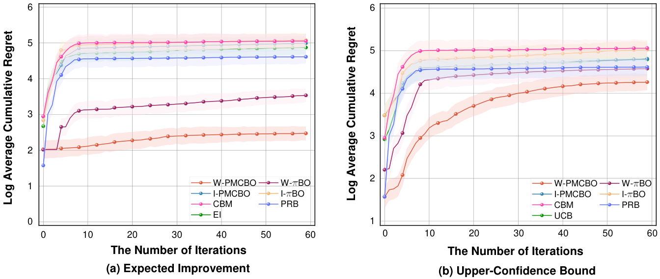
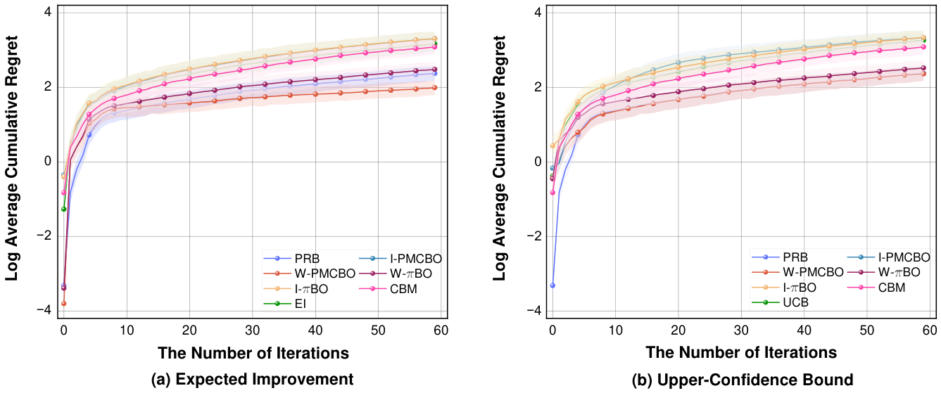
Performance of the Average Cumulative Regret: Primarily, we study the robustness of PMCBO based on cumulative regret. As shown in Figure 2, which compares the average cumulative regret (i.e., ${\displaystyle \frac{1}{L}}{\sum }_{l=1}^L{\sum }_{t=1}^T{r}_l^t$) across all clients based on the Branin function of the number of iterations T. We compare our PMCBO method based on two different acquisition strategies.

In the expected improvement acquisition function and its heuristic variants, as shown in Figure 2a, PMCBO (Wwak prior) can clearly outperform $\pi$BO (weak prior) and EI. Moreover, PMCBO (incorrect prior) initially samples points in the region far away from the optimum, and as the optimization process progresses, the prior acquisition function gradually decays to a normal acquisition function, and our method also has better performance compared with $\pi$BO (incorrect prior). In the upper-confidence bound acquisition function and its heuristic variants, Figure 2b, PMCBO (weak prior) can achieve the best performance. In the initial stage, all acquisition functions of BO methods aim to explore the unknown region of the Branin function; we specify the parameter ${\beta }_t=2log({\displaystyle \frac{t^{2}2{\pi }^2}{3\delta }})+2dlog(t^{2}dbr\sqrt{log({\displaystyle \frac{4da}{\delta }})})$, which results in the UCB and its heuristic variants’ acquisition functions tending to be more exploratory rather than exploitative compared to the EI and its heuristic variants. This result illustrates that $\pi$BO can rapidly adjust the region close to the optimum of Branin, while PMCBO can re-establish the trust region at a slightly measured pace. Furthermore, the cumulative regret of our method remains lower than that of other methods in Figure 2.

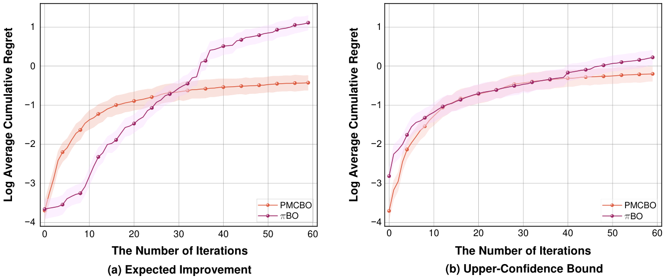
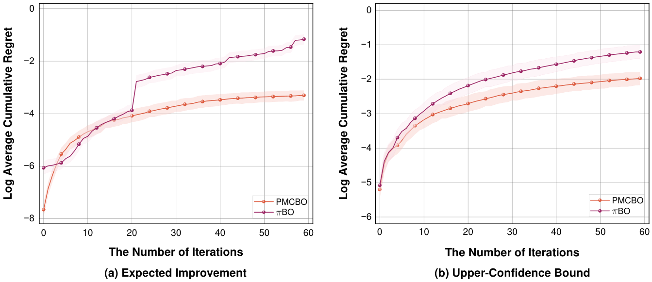
In addition, we utilize the same strong prior to compare the performance between our PMCBO method and the $\pi$BO. The value of the parameters for the strong prior are approximately $0.1$ away from the parameter values of the optimum and the standard deviation of the prior $0.01$, which ensures that the acquisition function prioritizes leveraging the expert prior knowledge rather than exploring unknown regions. As depicted in Figure 3, the PMCBO method incurs less cumulative regret than method of $\pi$BO with same strong prior.

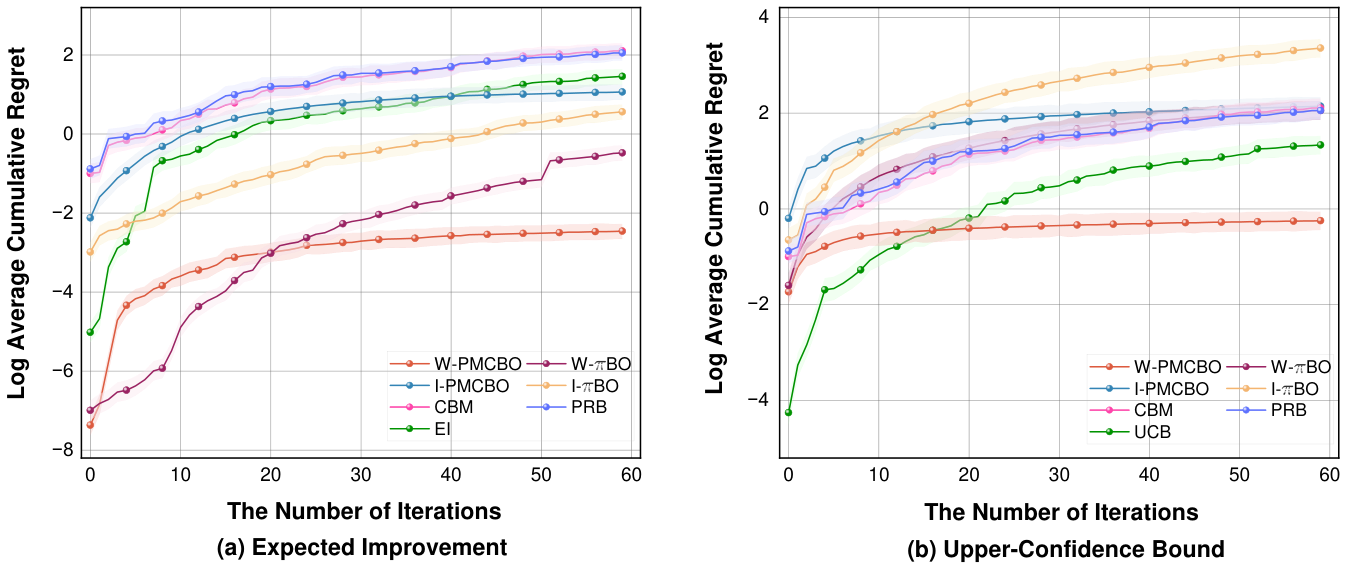
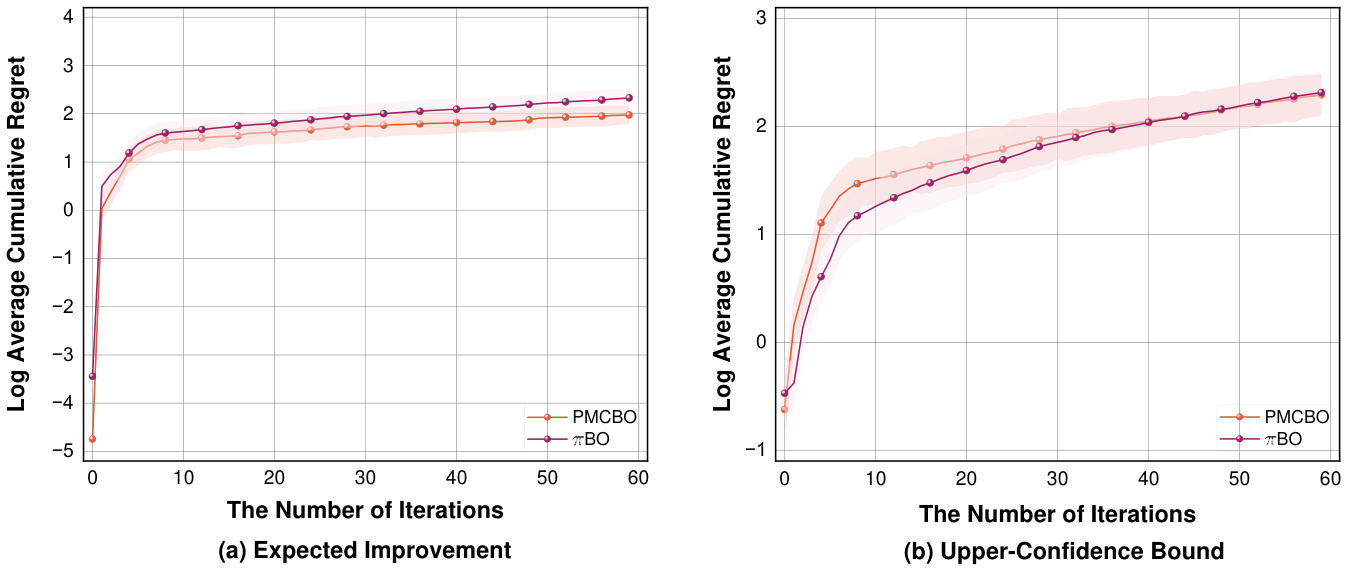
We also consider the other well-known benchmark optimization functions, specifically Hartman (3D) and Hartman (6D). Figure 4 and Figure 5 respectively demonstrate the logarithmic cumulative regret performance based on the function benchmark mentioned above. We observe that the PMCBO method exhibits superior performance compared to other BO methods that are depicted in Section 7.2. We also designed different expert prior knowledge for above two benchmark functions; the comparison results of the identical strong priors for the two benchmark functions are depicted in Figure 6 and Figure 7, respectively. We see that the proposed method can achieve a lower cumulative regret.

Performance of the Mean Average Simple Regret: We analyze the mean average simple regret (i.e., ${\displaystyle \frac{1}{TL}}{\sum }_{l=1}^L{\sum }_{t=1}^T{r}_l^t$) on benchmarks of Branin (2D), Hartman (3D) and Hartman (6D) around all clients in the DBO framework. For better readability, we cited references for the comparison methods and used boldface for our method. The regret performance of expected improvement acquisition function and its various heuristic versions are illustrated in

Table 4. Mean average simple regret across all clients on test benchmarks for baseline approaches in EI acquisition function and its heuristic variants.

Benchmark	Method	30 Iteration Simple Regret	60 Iteration Simple Regret
Branin	EI [6]	3.012	1.566
	CBM [40]	3.584	1.825
	PRB [43]	1.978	1.026
	S-PMCBO	0.0092	0.0059
	W-PMCBO	0.2973	0.1515
	I-PMCBO	3.4017	1.7091
	S-$\pi$BO [41]	0.0147	0.0071
	W-$\pi$BO [41]	0.475	0.2802
	I-$\pi$BO [41]	4.093	2.122
Hartman-3D	EI [6]	0.0274	0.0264
	CBM [40]	0.0485	0.053
	PRB [43]	0.069	0.055
	S-PMCBO	0.0005	0.0003
	W-PMCBO	0.0012	0.0007
	I-PMCBO	0.0599	0.03816
	S-$\pi$BO [41]	0.0014	0.0011
	W-$\pi$BO [41]	0.0065	0.0012
	I-$\pi$BO [41]	0.0160	0.0134
Hartman-6D	EI [6]	0.4097	0.3572
	CBM [40]	0.285	0.231
	PRB [43]	0.160	0.1274
	S-PMCBO	0.1344	0.0775
	W-PMCBO	0.1341	0.0813
	I-PMCBO	0.4641	0.4076
	S-$\pi$BO [41]	0.1782	0.1211
	W-$\pi$BO [41]	0.2026	0.1553
	I-$\pi$BO [41]	0.4630	0.4036

Note: Bold text indicates our proposed method; bold numbers denote the best performance.

. We separately analyze the mean average simple regret over the first 30 iterations and the mean average simple regret over the total number of iterations around all clients. From Table 4, the PMCBO method obviously outperforms other BO methods without priors. In addition, PMCBO can obtain greater performance compared with $\pi$BO. It is worth noting that the mean average simple regret of the entire set of iterations is lower than the regret of first 30 iterations. This is due to the strong priors we added causing the acquisition function to only sample near the optimal value; the acquisition function will still continuously explore the optimal value of the function.

Table 5. Mean average simple regret across all clients on test benchmarks for baseline approaches in UCB acquisition function and its heuristic variants.

Benchmark	Method	30 Iteration Simple Regret	60 Iteration Simple Regret
Branin	UCB [25]	2.625	1.400
	CBM [40]	3.584	1.825
	PRB [40]	1.978	1.026
	S-PMCBO	0.01367	0.01358
	W-PMCBO	1.0792	0.7371
	I-PMCBO	2.4425	1.3279
	S-$\pi$BO [41]	0.0325	0.02563
	W-$\pi$BO [41]	1.4819	0.819
	I-$\pi$BO [41]	3.0956	1.7232
Hartman-3D	UCB [25]	0.0289	0.0257
	CBM [40]	0.0485	0.053
	PRB [40]	0.069	0.055
	S-PMCBO	0.0022	0.0015
	W-PMCBO	0.02138	0.01162
	I-PMCBO	0.2020	0.1201
	S-$\pi$BO [41]	0.0045	0.0040
	W-$\pi$BO [41]	0.1376	0.1099
	I-$\pi$BO [41]	0.6593	0.6367
Hartman-6D	UCB [25]	0.4510	0.3925
	CBM [40]	0.285	0.231
	PRB [40]	0.16	0.1274
	S-PMCBO	0.1698	0.1213
	W-PMCBO	0.1596	0.1250
	I-PMCBO	0.5524	0.4228
	S-$\pi$BO [41]	0.1531	0.1195
	W-$\pi$BO [41]	0.2111	0.1621
	I-$\pi$BO [41]	0.4632	0.4024

Note: Bold text indicates our proposed method; bold numbers denote the best performance.

shows mean average simple regret of the upper-confidence bound acquisition function and its heuristic variants, where our PMCBO method with different priors can still demonstrate excellent performance on various benchmarks.

The current empirical evaluation is limited to synthetic benchmark functions under the homogeneous client setting. These controlled experiments are intended to isolate the effects of expert prior quality and collaborative information exchange. Extending PMCBO to heterogeneous or non-i.i.d. client objectives and validating it on application-specific tasks, such as hyperparameter optimization and engineering design, constitute important directions for future work.

8. Conclusions and Future Work

In this paper, we have proposed a PMCBO method for multiple clients within a distributed framework. PMCBO employs a Gaussian process as the surrogate model for each client-specific objective function and incorporates expert prior knowledge about the location of optimum into the acquisition function. Then, we primarily focus on prior-informed heuristic modifications for the two most well-known acquisition functions, i.e., EI and UCB. Once the posterior distribution is updated with the observations, the next query point is chosen by finding the maximum of an acquisition function. We analyze the performance of our algorithm with the regret, which is proportional to the RKHS norm between the objective function and the function-specific prior across all clients within the distributed framework. We have also taken into consideration the negative impact of an incorrect prior, which degrades the algorithm’s performance. To prevent this obstacle, we further propose a prior decay strategy to gradually reduce the influence of the prior on acquiring samples. The experimental results demonstrate the effectiveness of our PMCBO method in reducing the cost of regret. The current theoretical regret analysis and empirical evaluation mainly focus on homogeneous settings. Although this setting enables a controlled assessment of the prior-informed collaborative mechanism, it does not fully represent real distributed applications, in which clients may possess substantially different objective landscapes, evaluation costs, and noise characteristics. Therefore, the generalization of PMCBO to heterogeneous or non-i.i.d. clients remains to be theoretically and empirically investigated. Real-world applications, including distributed hyperparameter optimization and engineering design, will also be considered in future work.

References

1. Brochu, E.; Cora, V.M.; De Freitas, N. A tutorial on Bayesian optimization of expensive cost functions, with application to active user modeling and hierarchical reinforcement learning. arXiv 2010, arXiv:1012.2599. [Google Scholar] [CrossRef] [Scilit]
2. Shahriari, B.; Swersky, K.; Wang, Z.; Adams, R.P.; De Freitas, N. Taking the human out of the loop: A review of Bayesian optimization. Proc. IEEE 2015, 104, 148–175. [Google Scholar] [CrossRef] [Scilit]
3. Ru, B.; Alvi, A.; Nguyen, V.; Osborne, M.A.; Roberts, S. Bayesian optimisation over multiple continuous and categorical inputs. In Proceedings of the 37th International Conference on Machine Learning, PMLR, Virtual, 13–18 July 2020; pp. 8276–8285. [Google Scholar]
4. Garnett, R. Bayesian Optimization; Cambridge University Press: Cambridge, UK, 2023. [Google Scholar]
5. Pearce, M.; Branke, J. Continuous multi-task bayesian optimisation with correlation. Eur. J. Oper. Res. 2018, 270, 1074–1085. [Google Scholar] [CrossRef] [Scilit]
6. Snoek, J.; Larochelle, H.; Adams, R.P. Practical Bayesian Optimization of Machine Learning Algorithms. In Proceedings of the Advances in Neural Information Processing Systems, Lake Tahoe, NV, USA, 3–6 December 2012; Volume 25, pp. 2951–2959. [Google Scholar]
7. Fukazawa, T.; Harashima, Y.; Hou, Z.; Miyake, T. Bayesian optimization of chemical composition: A comprehensive framework and its application to R Fe12-type magnet compounds. Phys. Rev. Mater. 2019, 3, 053807. [Google Scholar] [CrossRef] [Scilit]
8. Bergstra, J.; Bardenet, R.; Bengio, Y.; Kégl, B. Algorithms for hyper-parameter optimization. In Proceedings of the Advances in Neural Information Processing Systems, Granada, Spain, 12–15 December 2011; Volume 24, pp. 2546–2554. [Google Scholar]
9. Klein, A.; Hutter, F. Tabular benchmarks for joint architecture and hyperparameter optimization. arXiv 2019, arXiv:1905.04970. [Google Scholar] [CrossRef] [Scilit]
10. Wang, H.; Zhang, X.; Ng, S.H. A nonparametric Bayesian approach for simulation optimization with input uncertainty. arXiv 2020, arXiv:2008.02154. [Google Scholar] [CrossRef] [Scilit]
11. Chen, T.; Guestrin, C. Xgboost: A scalable tree boosting system. In Proceedings of the 22nd ACM Sigkdd International Conference on Knowledge Discovery and Data Mining, San Francisco, CA, USA, 13–17 August 2016; pp. 785–794. [Google Scholar] [CrossRef] [Scilit]
12. Griffiths, R.R.; Hernández-Lobato, J.M. Constrained Bayesian optimization for automatic chemical design using variational autoencoders. Chem. Sci. 2020, 11, 577–586. [Google Scholar] [CrossRef] [Scilit] [PubMed]
13. Eric, B.; Freitas, N.; Ghosh, A. Active preference learning with discrete choice data. In Proceedings of the Advances in Neural Information Processing Systems, Vancouver, BC, Canada, 3–6 December 2007; Volume 20, pp. 409–416. [Google Scholar]
14. Koyama, Y.; Sato, I.; Sakamoto, D.; Igarashi, T. Sequential line search for efficient visual design optimization by crowds. ACM Trans. Graph. (TOG) 2017, 36, 48. [Google Scholar] [CrossRef] [Scilit]
15. Calandra, R.; Seyfarth, A.; Peters, J.; Deisenroth, M.P. Bayesian optimization for learning gaits under uncertainty: An experimental comparison on a dynamic bipedal walker. Ann. Math. Artif. Intell. 2016, 76, 5–23. [Google Scholar] [CrossRef] [Scilit]
16. Attia, P.M.; Grover, A.; Jin, N.; Severson, K.A.; Markov, T.M.; Liao, Y.H.; Chen, M.H.; Cheong, B.; Perkins, N.; Yang, Z.; et al. Closed-loop optimization of fast-charging protocols for batteries with machine learning. Nature 2020, 578, 397–402. [Google Scholar] [CrossRef] [Scilit] [PubMed]
17. Hutter, F.; Hoos, H.H.; Leyton-Brown, K. Sequential Model-Based Optimization for General Algorithm Configuration. In Learning and Intelligent Optimization; Lecture Notes in Computer Science; Springer: Berlin/Heidelberg, Germany, 2011; pp. 507–523. [Google Scholar] [CrossRef] [Scilit]
18. Rasmussen, C.E.; Williams, C.K. Gaussian Processes for Machine Learning; The MIT Press: Cambridge, MA, USA, 2006. [Google Scholar] [CrossRef] [Scilit]
19. Springenberg, J.T.; Klein, A.; Falkner, S.; Hutter, F. Bayesian optimization with robust Bayesian neural networks. In Proceedings of the Advances in Neural Information Processing Systems, Barcelona, Spain, 5–10 December 2016; Volume 29, pp. 4141–4149. [Google Scholar]
20. Li, Y.L.; Rudner, T.G.; Wilson, A.G. A Study of Bayesian Neural Network Surrogates for Bayesian Optimization. In Proceedings of the 12nd International Conference on Learning Representations, Vienna, Austria, 7–11 May 2024. [Google Scholar]
21. Wang, Z.; Gehring, C.; Kohli, P.; Jegelka, S. Batched large-scale Bayesian optimization in high-dimensional spaces. In Proceedings of the 21st International Conference on Artificial Intelligence and Statistics, PMLR, Playa Blanca, Lanzarote, Canary Islands, Spain, 9–11 April 2018; pp. 745–754. [Google Scholar]
22. Kushner, H. A New Method of Locating the Maximum Point of an Arbitrary Multipeak Curve in the Presence of Noise. J. Basic Eng. 1964, 86, 97–106. [Google Scholar] [CrossRef] [Scilit]
23. Mockus, J.; Tiesis, V.; Zilinskas, A. The application of Bayesian methods for seeking the extremum. Towards Glob. Optim. 1998, 2, 117–129. [Google Scholar] [CrossRef] [Scilit]
24. Frazier, P.I.; Powell, W.B.; Dayanik, S. A knowledge-gradient policy for sequential information collection. SIAM J. Control Optim. 2008, 47, 2410–2439. [Google Scholar] [CrossRef] [Scilit]
25. Srinivas, N.; Krause, A.; Kakade, S.M.; Seeger, M.W. Information-theoretic regret bounds for gaussian process optimization in the bandit setting. IEEE Trans. Inf. Theory 2012, 58, 3250–3265. [Google Scholar] [CrossRef] [Scilit]
26. Hennig, P.; Schuler, C.J. Entropy Search for Information-Efficient Global Optimization. J. Mach. Learn. Res. 2012, 13, 1809–1837. [Google Scholar]
27. Hernández-Lobato, J.M.; Hoffman, M.W.; Ghahramani, Z. Predictive entropy search for efficient global optimization of black-box functions. In Proceedings of the Advances in Neural Information Processing Systems, Montreal, QC, Canada, 8–13 December 2014; Volume 27, pp. 918–926. [Google Scholar]
28. Wang, Z.; Jegelka, S. Max-value entropy search for efficient Bayesian optimization. In Proceedings of the 34th International Conference on Machine Learning, PMLR, Sydney, Australia, 6–11 August 2017; pp. 3627–3635. [Google Scholar]
29. Wu, J.; Frazier, P. Practical two-step lookahead Bayesian optimization. In Proceedings of the Advances in Neural Information Processing Systems, Vancouver, BC, Canada, 8–14 December 2019; Volume 32, pp. 9813–9823. [Google Scholar]
30. Swersky, K.; Snoek, J.; Adams, R.P. Multi-task Bayesian optimization. In Proceedings of the Advances in Neural Information Processing Systems, Lake Tahoe, NV, USA, 5–8 December 2013; pp. 2004–2012. [Google Scholar]
31. Chowdhury, S.R.; Gopalan, A. No-regret Algorithms for Multi-task Bayesian Optimization. In Proceedings of the 24th International Conference on Artificial Intelligence and Statistics, PMLR, Virtual, 13–15 April 2021; pp. 1873–1881. [Google Scholar]
32. Wu, X.; Niu, J.; Liu, X.; Zhu, G.; Tang, S.; Lin, W.; Cao, J. The Diversity Bonus: Learning From Dissimilar Clients in Personalized Federated Learning. IEEE Trans. Neural Netw. Learn. Syst. 2025, 36, 18613–18627. [Google Scholar] [CrossRef] [Scilit] [PubMed]
33. Zhang, Q.; Tan, Y.S.; Chen, J. Byzantine-tolerant distributed learning of finite mixture models. J. R. Stat. Soc. B 2026, qkag065. [Google Scholar] [CrossRef] [Scilit]
34. Li, T.; Sahu, A.K.; Talwalkar, A.; Smith, V. Federated learning: Challenges, methods, and future directions. IEEE Signal Process. Mag. 2020, 37, 50–60. [Google Scholar] [CrossRef] [Scilit]
35. Smith, L.N. A disciplined approach to neural network hyper-parameters: Part 1–learning rate, batch size, momentum, and weight decay. arXiv 2018, arXiv:1803.09820. [Google Scholar] [CrossRef] [Scilit]
36. Wang, Z.; Kim, B.; Kaelbling, L.P. Regret bounds for meta Bayesian optimization with an unknown Gaussian process prior. In Proceedings of the Advances in Neural Information Processing Systems, Montréal, QC, Canada, 3–8 December 2018; pp. 10498–10509. [Google Scholar]
37. Anand, K.; Wang, Z.; Loog, M.; van Gemert, J. Black magic in deep learning: How human skill impacts network training. arXiv 2020, arXiv:2008.05981. [Google Scholar] [CrossRef] [Scilit]
38. Wang, Q.; Ming, Y.; Jin, Z.; Shen, Q.; Liu, D.; Smith, M.J.; Veeramachaneni, K.; Qu, H. Atmseer: Increasing transparency and controllability in automated machine learning. In Proceedings of the 37th CHI Conference on Human Factors in Computing Systems, Glasgow, UK, 4–9 May 2019; pp. 1–12. [Google Scholar] [CrossRef] [Scilit]
39. Souza, A.; Nardi, L.; Oliveira, L.B.; Olukotun, K.; Lindauer, M.; Hutter, F. Bayesian Optimization with a Prior for the Optimum. In Proceedings of the 31st Joint European Conference on Machine Learning and Knowledge Discovery in Databases, Bilbao, Spain, 13–17 September 2021; pp. 265–296. [Google Scholar] [CrossRef] [Scilit]
40. Nguyen, V.; Osborne, M.A. Knowing the what but not the where in Bayesian optimization. In Proceedings of the the 37th International Conference on Machine Learning, PMLR, Virtual, 12–18 July 2020; pp. 7317–7326. [Google Scholar]
41. Hvarfner, C.; Stoll, D.; Souza, A.; Lindauer, M.; Hutter, F.; Nardi, L. πBO: Augmenting Acquisition Functions with User Beliefs for Bayesian Optimization. In Proceedings of the 10th International Conference of Learning Representations, Virtual, 25–29 April 2022. [Google Scholar]
42. Yue, X.; Liu, Y.; Berahas, A.S.; Johnson, B.N.; Al Kontar, R. Collaborative and Distributed Bayesian Optimization via Consensus. IEEE Trans. Autom. Sci. Eng. 2025, 22, 11343–11355. [Google Scholar] [CrossRef] [Scilit]
43. Wilson, J.T. Stopping Bayesian Optimization with Probabilistic Regret Bounds. In Proceedings of the Advances in Neural Information Processing Systems, Vancouver, BC, Canada, 10–15 December 2024; Volume 37, pp. 98264–98296. [Google Scholar]
44. Ocenasek, J.; Schwarz, J. The distributed Bayesian optimization algorithm for combinatorial optimization. In EUROGEN-Evolutionary Methods for Design, Optimisation and Control; COMSOL, Inc.: Burlington, MA, USA, 2001; pp. 115–120. [Google Scholar]
45. Garcia-Barcos, J.; Martinez-Cantin, R. Fully distributed bayesian optimization with stochastic policies. In Proceedings of the 28th International Joint Conference on Artificial Intelligence, Macao, China, 10–16 August 2019; pp. 2357–2363. [Google Scholar] [CrossRef] [Scilit] [PubMed]
46. Na, Y.; Yang, J. Distributed Bayesian network structure learning. In Proceedings of the 19th IEEE International Symposium on Industrial Electronics, Bari, Italy, 4–7 July 2010; pp. 1607–1611. [Google Scholar] [CrossRef] [Scilit]
47. Egelé, R.; Guyon, I.; Vishwanath, V.; Balaprakash, P. Asynchronous decentralized bayesian optimization for large scale hyperparameter optimization. In Proceedings of the 19th International Conference on e-Science, Limassol, Cyprus, 9–13 October 2023; pp. 1–10. [Google Scholar] [CrossRef] [Scilit]
48. Tang, W.; Li, J.; Chen, L.; Chen, X. Design and Optimization of Hierarchical Gradient Coding for Distributed Learning at Edge Devices. IEEE Trans. Commun. 2024, 72, 7727–7741. [Google Scholar] [CrossRef] [Scilit]
49. Hakhamaneshi, K.; Abbeel, P.; Stojanovic, V.; Grover, A. Jumbo: Scalable multi-task bayesian optimization using offline data. arXiv 2021, arXiv:2106.00942. [Google Scholar] [CrossRef] [Scilit]
50. Wistuba, M.; Grabocka, J. Few-Shot Bayesian Optimization with Deep Kernel Surrogates. In Proceedings of the 8th International Conference on Learning Representations, Virtual, 26 April–1 May 2020. [Google Scholar] [CrossRef]
51. Volpp, M.; Fröhlich, L.P.; Fischer, K.; Doerr, A.; Falkner, S.; Hutter, F.; Daniel, C. Meta-Learning Acquisition Functions for Transfer Learning in Bayesian Optimization. In Proceedings of the 7th International Conference on Learning Representations, New Orleans, LA, USA, 6–9 May 2019. [Google Scholar]
52. Perrone, V.; Jenatton, R.; Seeger, M.W.; Archambeau, C. Scalable hyperparameter transfer learning. In Proceedings of the Advances in Neural Information Processing Systems, Montréal, QC, Canada, 3–8 December 2018; Volume 31, pp. 6846–6856. [Google Scholar]
53. Wang, Z.; Dahl, G.E.; Swersky, K.; Lee, C.; Nado, Z.; Gilmer, J.; Snoek, J.; Ghahramani, Z. Pre-trained Gaussian Processes for Bayesian Optimization. J. Mach. Learn. Res. 2024, 25, 1–83. [Google Scholar] [CrossRef] [Scilit]
54. Oh, C.; Gavves, E.; Welling, M. BOCK: Bayesian optimization with cylindrical kernels. In Proceedings of the 35th International Conference on Machine Learning, PMLR, Stockholm, Sweden, 10–15 July 2018; pp. 3868–3877. [Google Scholar]
55. Siivola, E.; Vehtari, A.; Vanhatalo, J.; González, J.; Andersen, M.R. Correcting boundary over-exploration deficiencies in Bayesian optimization with virtual derivative sign observations. In Proceedings of the 28th International Workshop on Machine Learning for Signal Processing, Aalborg, Denmark, 17–20 September 2018; pp. 1–6. [Google Scholar] [CrossRef] [Scilit]
56. Ramachandran, A.; Gupta, S.; Rana, S.; Li, C.; Venkatesh, S. Incorporating expert prior in Bayesian optimisation via space warping. Knowl.-Based Syst. 2020, 195, 105663. [Google Scholar] [CrossRef] [Scilit]
57. Porcu, E.; Bevilacqua, M.; Schaback, R.; Oates, C.J. The Matérn model: A journey through statistics, numerical analysis and machine learning. Stat. Sci. 2024, 39, 469–492. [Google Scholar] [CrossRef] [Scilit]
58. Cover, T.M.; Thomas, J.A. Elements of Information Theory, 2nd ed.; Wiley Interscience: Hoboken, NJ, USA, 2006. [Google Scholar]
59. Auer, P. Using confidence bounds for exploitation-exploration trade-offs. J. Mach. Learn. Res. 2002, 3, 397–422. [Google Scholar]
60. Poonawala, H.A.; Spong, M.W. Decentralized estimation of the algebraic connectivity for strongly connected networks. In Proceedings of the 34th American Control Conference, Chicago, IL, USA, 1–3 July 2015; pp. 4068–4073. [Google Scholar] [CrossRef] [Scilit]
61. Chowdhury, S.R.; Gopalan, A. On kernelized multi-armed bandits. In Proceedings of the 34th International Conference on Machine Learning, PMLR, Sydney, Australia, 6–11 August 2017; pp. 844–853. [Google Scholar]
62. Wahba, G. Spline Models for Observational Data; SIAM: Bangkok, Thailand, 1990. [Google Scholar] [CrossRef] [Scilit]
63. Shi, X.; Cao, J.; Huang, W. Distributed parametric consensus optimization with an application to model predictive consensus problem. IEEE Trans. Cybern. 2017, 48, 2024–2035. [Google Scholar] [CrossRef] [Scilit] [PubMed]
64. Berahas, A.S.; Bollapragada, R.; Keskar, N.S.; Wei, E. Balancing communication and computation in distributed optimization. IEEE Trans. Autom. Control 2018, 64, 3141–3155. [Google Scholar] [CrossRef] [Scilit]
65. Srinivas, N.; Krause, A.; Kakade, S.; Seeger, M. Gaussian Process Optimization in the Bandit Setting: No Regret and Experimental Design. In Proceedings of the 27th International Conference on Machine Learning, Haifa, Israel, 21–24 June 2010; pp. 1015–1022. [Google Scholar]
66. Bull, A.D. Convergence Rates of Efficient Global Optimization Algorithms. J. Mach. Learn. Res. 2011, 12, 2879–2904. [Google Scholar]
67. Jamil, M.; Yang, X.-S. A literature survey of benchmark functions for global optimization problems. arXiv 2013, arXiv:1308.4008. [Google Scholar] [CrossRef] [Scilit]
Figure 1. Overview of the proposed PMCBO framework.
Mathematics 14 03040 g001
Figure 2. Logarithmic average cumulative regret comparison of baseline methods for Branin (2D) benchmark. The line and shaded regions show mean and standard deviations.
Mathematics 14 03040 g002
Figure 3. Logarithmic average cumulative regret comparison for Branin (2D) benchmark with the same strong prior. The line and shaded regions show mean and standard deviations.
Mathematics 14 03040 g003
Figure 4. Logarithmic average cumulative regret comparison of baseline methods for Hartman (3D) benchmark. The line and shaded regions show mean and standard deviations.
Mathematics 14 03040 g004
Figure 5. Logarithmic average cumulative regret comparison of baseline methods for Hartman (6D) benchmark. The line and shaded regions show mean and standard deviations.
Mathematics 14 03040 g005
Figure 6. Logarithmic average cumulative regret comparison for Hartman (3D) benchmark with the same strong prior. The line and shaded regions show mean and standard deviations.
Mathematics 14 03040 g006
Figure 7. Logarithmic average cumulative regret comparison for Hartman (6D) benchmark with the same strong prior. The line and shaded regions show mean and standard deviations.
Mathematics 14 03040 g007