Article

Anatolian Caracal Optimization Algorithm: A Three-Stage Hybrid Bio- and Physics-Inspired Framework for Optimization Problems


1
Department of Computer Engineering, İnönü University, Malatya 44280, Türkiye
2
Department of Computer Engineering, Malatya Turgut Özal University, Malatya 44920, Türkiye
3
Department of Electrical and Electronics Engineering, İnönü University, Malatya 44280, Türkiye
4
Department of Electrical and Electronics Engineering, Istinye University, İstanbul 34396, Türkiye
*
Author to whom correspondence should be addressed.
Mathematics 2026, 14(16), 3007; https://doi.org/10.3390/math14163007
Submission received: 18 June 2026 / Revised: 28 July 2026 / Accepted: 4 August 2026 / Published: 20 August 2026

Abstract

The Anatolian Caracal Optimization Algorithm (ACOA), a swarm-based optimization approach inspired by nature, approximately describes the characteristic hunting strategy of the Anatolian caracal, shaped by its superior auditory–visual perception and extraordinary agility, using mathematical models. The algorithm structures this process into three main stages by integrating and modifying established search mechanisms within a sequential framework: (i) wide-area scanning (exploration), which supports a broad exploration of the solution space through prey-focused movements; (ii) tracking–approach, which uses Brownian (continuous, small steps) and Lévy (occasional long jumps) movements to support the transition from exploration to exploitation; and (iii) predatory leap (exploitation), which represents the Anatolian caracal’s jump with a dimensionless projectile-inspired formulation and supports the refinement of candidate solutions. ACOA has been benchmarked across the CEC 2017, CEC 2019, CEC 2020, and CEC 2022 test suites, including unimodal and multimodal functions with fixed and varying dimensions, as well as real-world engineering design problems, for a total of 131 functions. It has been compared against 11 recent and well-known optimization algorithms. The best mean performance is achieved by ACOA in 111 out of 131 cases. In terms of stability, consistently low standard deviation is maintained by ACOA across the majority of the evaluated functions, indicating a strong reproducibility of the obtained solutions across independent runs. These findings indicate that the proposed three-stage framework provides a competitive exploration–exploitation behavior and can offer effective and stable solutions for a wide range of benchmark and engineering optimization problems.

1. Introduction

Optimization refers to the process of obtaining the best solution among all feasible solutions for an engineering (or different mathematical) problem. For a problem to be classified as an optimization problem, it must contain three basic components: constraints, decision variables, and an objective function [1,2]. During the optimization process, appropriate values are assigned to the decision variables, and the objective function is optimized subject to the given constraints [2]. In the literature, general approaches to solving optimization problems are categorized into two main groups: deterministic and stochastic algorithms. Deterministic algorithms are mathematical methods that consistently yield the same solution when provided with identical input data. Examples of deterministic algorithms include Integer Programming (IP) [3], Nonconvex Nonlinear Programming (NNLP) [4], and Mixed-Integer Nonlinear Programming (MINLP) [5]. In contemporary practice, most real-world engineering problems involve numerous constraints and require the optimization of a large number of control variables. Deterministic algorithms often fail to provide satisfactory solutions for such problems. Consequently, the use of stochastic algorithms in optimization has gained popularity. Stochastic algorithms are further divided into two subcategories: heuristic and metaheuristic. Heuristic algorithms search for near-optimal solutions through a trial-and-error process [6]. Metaheuristic algorithms, on the other hand, offer several advantages, including the incorporation of randomness and their applicability to a wide range of problems, serving as an alternative to traditional mathematical methods. In this respect, they address the shortcomings of deterministic approaches. A metaheuristic algorithm typically begins by assigning a random initial value to the problem. In subsequent iterations, the algorithm explores the solution space through mutation, receptor editing, and local search mechanisms [7]. With recent technological advancements, optimization algorithms have found applications in numerous fields, including image processing [8], load flow analysis in power systems [9], protection coordination in power systems [10], artificial intelligence [11], biomedical engineering [12], civil engineering [13], green production and production planning [14], pattern recognition [15], and electric vehicles [16]. In such areas, optimization algorithms can enhance computational efficiency for complex engineering problems and reduce overall costs. Due to the inherently complex nature of these problems, metaheuristic algorithms have gained significant popularity. One of the most important advantages offered by metaheuristic algorithms is that they do not require prior knowledge of the mathematical properties of the objective function [17]. However, despite these benefits, they also have certain drawbacks. The most notable disadvantages include high sensitivity to control parameter variations, premature convergence, and the tendency to become trapped in local minima [18]. In the literature, metaheuristic algorithms are categorized into various groups based on their characteristics, with four main classifications being the most common.
  • Algorithms inspired by evolutionary processes
  • Game-based algorithms
  • Physics-based algorithms
  • Swarm-based algorithms
Evolutionary algorithms are often designed with inspiration from biological evolutionary processes. Over the past 15–20 years, these algorithms have proven effective in solving high-dimensional and nonlinear problems. Examples of this group include the Genetic Algorithm (GA) [19], the Artificial Immune System Algorithm (AIAL) [20], and the Differential Evolution Algorithm [21]. Game-based metaheuristic algorithms are inspired by the principles of game theory, utilizing simple rules to guide their operations. Examples include the Golf Optimization Algorithm [22], the Billiards Optimization Algorithm [23], Shell Game Optimization [24], the Skill Optimization Algorithm [25], and the Football Game Algorithm [26]. Physics-based algorithms are optimization methods inspired by natural phenomena observed in physical systems. These algorithms aim to reach the global optimum by drawing on the laws of force, motion, energy exchange, and thermodynamics found in nature. These algorithms translate selected physical principles into mathematical search operators intended to support exploration and exploitation. Examples of physics-based metaheuristic algorithms include the Archimedes Optimization Algorithm (AOA) [27], the Big Bang–Big Crunch Optimization Algorithm [28], the Gravitational Search Algorithm (GSA) [29], the Electrostatic Discharge Algorithm (ESDA) [30], and the Electromagnetic Field Optimization Algorithm [31]. Swarm-based metaheuristic algorithms are developed based on inspiration from natural collective behaviors, particularly those observed in insects, animals, and other living organisms. Examples include the Particle Swarm Optimization Algorithm (PSO) [32], Whale Optimization Algorithm [33], Butterfly Optimization Algorithm [34], Honey Badger Algorithm (HBA) [35], Cuckoo Optimization Algorithm (COA) [36], Chimp Optimization Algorithm (ChOA) [37], Spider Monkey Optimization Algorithm (SMOA) [38], Forest Optimization Algorithm [39], Grasshopper Optimization Algorithm [40], Zebra Optimization Algorithm [41], Crayfish Optimization Algorithm [42], Coati Optimization Algorithm [43], Prairie Dog Optimization Algorithm [44], Red Fox Optimization Algorithm [45], Harris Hawks Optimization Algorithm [46], Horse Herd Optimization Algorithm [47], Hippopotamus Optimization Algorithm [48], Tasmanian Devil Optimization [49], Artificial Bee Colony (ABC) Optimization [50], Osprey Optimization Algorithm [51], Swallow Swarm Optimization Algorithm [52], Marine Predators Algorithm [53], Grey Wolf Optimization Algorithm [54], Cat Swarm Optimization Algorithm [55], Lion Optimization Algorithm [56], and Pelican Optimization Algorithm [57].
More recently, a distinct family of parameter-less and metaphor-free algorithms has emerged, aiming to eliminate algorithm-specific control parameters entirely, such as the Best-Mean-Random (BMR) and Best-Worst-Random (BWR) algorithms [58], which rely solely on the best, mean, worst, and random solutions of the population. These algorithms have since been applied to manufacturing process optimization [59] and heat transfer system design [60], and have been comprehensively surveyed by Beldar and Rao [61], who classify optimization algorithms according to their dependence on tunable control parameters.
Metaheuristic algorithms may occasionally fail to guarantee the best solution. Since the solutions they produce are generally close to the global optimum, such results are often accepted as satisfactory solutions. However, because their algorithmic structure is based on mathematical equations generated through random processes, they cannot ensure convergence to the true global optimum. For metaheuristic algorithms to successfully produce feasible solutions to optimization problems, they must effectively explore both the global and local search spaces. The search process consists of two main components: exploration and exploitation. Exploration enables a broad, global search of the solution space, reducing the likelihood of premature convergence to local optima and increasing the likelihood of discovering superior solutions. Exploitation, on the other hand, focuses on intensive search within the local space, aiming to refine promising areas and move closer to the global optimum. The effective performance of an optimization algorithm depends on maintaining a proper balance between exploration and exploitation. Although dozens of optimization algorithms exist today, the No Free Lunch (NFL) theorem [62] clearly explains the motivation for developing new ones. The NFL theorem states that an optimization algorithm that performs well on one problem will inevitably perform poorly on another and will, in general, be prone to becoming trapped in local optima. Therefore, there is no guarantee that a metaheuristic algorithm effective for one problem will be equally effective for another. At this point, the NFL theorem and previous studies on the subject encourage researchers to continuously develop new metaheuristic optimization algorithms. In line with this principle, the present study introduces the Anatolian Caracal Optimization Algorithm (ACOA), a three-stage swarm-based optimization framework inspired by the hunting behavior of the Anatolian caracal. The proposed framework integrates and modifies established search mechanisms within a sequential wide-area scanning, tracking–approach, and predatory-leap structure.
The Anatolian caracal (Caracal caracal), which forms the biological inspiration for ACOA, is a predatory species with high ecological adaptability and a broad distribution across the Mediterranean region of Türkiye. This species exhibits a distinctive hunting strategy characterized by a multistage process of detecting, approaching, and leaping to capture prey. This behavior is indicative of advanced cognitive capabilities. The caracal has been described as an adaptive and generalist predator with broad ecological tolerance. However, habitat loss, including the degradation of forest and maquis vegetation in fire-affected areas, may negatively affect its population [63,64]. In this study, the strategic hunting behavior and remarkable adaptability of the Anatolian caracal were modeled within the framework of nature-inspired computational approaches, leading to the development of the ACOA algorithm.
Specifically, this study targets high-dimensional, multimodal, and constrained real-parameter optimization problems that are difficult for gradient-based and single-strategy metaheuristic methods to solve reliably. This problem class is exemplified in the present work by constrained mechanical/structural engineering design problems (e.g., pressure vessel design, welded beam design, speed reducer design) and by power distribution network planning, specifically the optimal placement of electric vehicle charging stations (EVCS) on the IEEE 33-bus and 69-bus test systems.
The main features of the Anatolian Caracal Optimization Algorithm are as follows:
Multi-Stage Exploration and Scanning Mechanism: Inspired by the Anatolian caracal’s wide-range prey search behavior, ACOA adopts a structure that supports the investigation of different regions of the solution space.
Adaptive Convergence Strategy: Once it detects its prey, the Anatolian caracal systematically reduces the distance to reach the optimal attack position (using Lévy and Brownian movements). This process is integrated into the algorithm as an adaptive mechanism that supports the progressive adjustment of the search process.
Dynamic Attack Mechanism: In response to the prey’s escape movements, the Anatolian caracal leaps to capture it. In ACOA, this feature is modeled as the ability to make sudden directional changes and improve solutions during the local search process.
Exploration–Exploitation Balance: ACOA has been developed as an algorithm that is designed to coordinate exploration- and exploitation-oriented movements. This enables it to efficiently evaluate a wide solution space with the aim of reducing the risk of premature convergence. ACOA is proposed based on a three-stage mathematical framework.

2. Inspiration

The caracal (Caracal caracal) is a feline species with a lynx-like appearance. The name caracal is derived from the Turkish word karakulak [65]. Adult males typically weigh between 12 and 18 kg, while females range from 8 to 13 kg. The body length generally measures between 75 and 90 cm. Figure 1 presents an image of an Anatolian caracal captured using camera traps. The Anatolian caracal belongs to the subspecies Caracal schmitzi, a member of the Caracal genus. This subspecies inhabits the Mediterranean region of Türkiye, with its population estimated at approximately 3000 individuals. Although the Anatolian caracal is predominantly a solitary hunter, ACOA adopts a population-based search paradigm common to nearly all swarm-inspired metaheuristics, in which each candidate solution independently explores the search space using the caracal’s hunting strategy as a shared behavioral template, analogous to how single-agent biological behaviors (e.g., grey wolf, whale) are routinely modeled through multi-agent populations in the optimization literature. This modeling convention is well established for other solitary-hunting species as well; for instance, the Honey Badger Algorithm [35], the Red Fox Optimization Algorithm [45], the Osprey Optimization Algorithm [51], Tasmanian Devil Optimization [49], and the Pelican Optimization Algorithm [57] all formulate the foraging or hunting behavior of fundamentally solitary animals within a population-based swarm framework. ACOA follows this same established practice.
Similar to other large felids, the Anatolian caracal plays a significant role in its surrounding ecosystem. As a predator, it helps regulate herbivore populations and is notable for its distinctive hunting strategies, which include both terrestrial and aerial hunting capabilities [66]. Agile and powerful, the Anatolian caracal is particularly adapted to preying on small and medium-sized mammals as well as birds. Its physical prowess, especially its exceptional leaping ability and prey-tracking skills, distinguishes it from many other predatory cats [67]. Owing to its unique hunting strategy and remarkable adaptability to environmental conditions, the Anatolian caracal served as the primary inspiration for the development of ACOA.

Anatolian Caracal: Superior Hunting Strategy

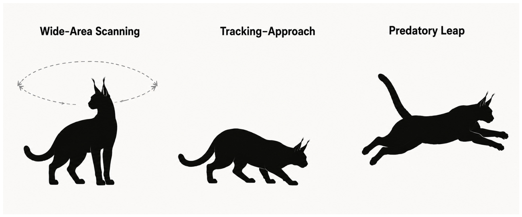
The Anatolian caracal is a keystone species, playing a vital role in maintaining prey–population balance within its ecosystem through its exceptional hunting skills [66]. Its high intelligence and remarkable physical abilities provide valuable inspiration for designing optimization approaches that balance exploration and exploitation. Research indicates that the hunting process of the Anatolian caracal comprises three main stages (Figure 2):
  • Wide-Area Scanning: The Anatolian caracal locates its prey by systematically scanning an extensive area. Male individuals typically cover up to 20 km, whereas females search within a range of 5–10 km. Their exceptionally keen hearing and vision enable them to detect even the slightest movements. In the context of optimization, this behavior can be modeled as a broad exploration of the solution space, helping to avoid entrapment in local optima.
  • Tracking–Approach: Before launching a direct attack, the Anatolian caracal strategically utilizes environmental features to reduce the distance to its prey. The Anatolian caracal may sometimes approach in a continuous, smooth motion and, at other times, make sudden advances in short leaps, depending on the prey’s behavior [66,67,68,69]. These movement patterns closely resemble Brownian and Lévy motions, which form the basis of stochastic processes. These stochastic processes are used as computational abstractions; they are not claimed to be empirically identified movement distributions of the Anatolian caracal.
  • Predatory Leap: The Anatolian caracal captures its prey by executing a rapid and powerful leap in response to sudden escape maneuvers. Its ability to catch birds, particularly those fleeing mid-air, is one of its most remarkable hunting strategies and is closely linked to its rapid and precise decision-making capabilities [66]. In the context of optimization, this behavior can be likened to dynamically reaching the optimal point in the solution space. This process exhibits a dynamic structure that is physically analogous to the mathematical model of projectile motion. When closing in on its prey, the caracal optimizes the initial velocity components and accounts for gravitational effects to determine the most efficient leap angle, thereby maximizing target acquisition time and accuracy. Moreover, its ability to adaptively select its escape trajectory and adjust its path based on the prey’s movement dynamics highlights its capacity to respond swiftly to environmental changes. This adaptive capability mirrors a search strategy in optimization processes that adjusts to changing conditions and accelerates convergence to the target point in the solution space.
This multi-stage hunting strategy allows the ACOA algorithm to adapt the exploration and exploitation processes in a balanced and systematic manner, drawing inspiration from nature. Given the necessity of effectively managing multiple decision variables in solving complex engineering problems, ACOA is designed to balance exploration and exploitation through its dynamic, physics-inspired structure. To this end, the strategic hunting mechanisms of the Anatolian caracal, which has a high hunting success rate in its natural environment, were modeled as the primary inspiration for the algorithm.

3. Anatolian Caracal Optimization Algorithm (ACOA)

ACOA is a population-based algorithm in which caracals are members of a population of interest. As in other population-based algorithms, each caracal in the population represents a candidate solution. Each caracal proposes values for the variables in the optimization problem based on its current location in the search space. ACOA simulates the superior hunting strategy of the Anatolian caracal, described in the previous section, in three stages. In the first strategy, a caracal attempts to locate prey across a wide area. In the second strategy, the prey’s location is detected through scent, visual cues, or sound, and the predator approaches the prey in a controlled manner using continuous, smooth movements or small jumps. This process is modeled as a simulation of predator–prey interactions. In the third strategy, a caracal attempts to leap onto its prey and capture it. In this study, ACOA utilizes exploration and exploitation mechanisms. The first strategy simulates exploration behavior, while the second and third strategies represent exploitation behavior. As in other population-based metaheuristic algorithms, ACOA begins the search process with a candidate solution. Subsequently, each individual is evaluated according to the objective function.

3.1. Mathematical Model of ACOA

As previously explained, ACOA is divided into three phases: ‘wide-area scanning’, ‘tracking–approach’, and ‘predatory leap’, which are detailed below:
Initialization: The initial population is calculated according to the number of Anatolian caracals ( N ) and the lower and upper limits of the population problem (Equation (1)).
X i , j = L B j + r 1 ( U B j L B j )   i = 1 , 2 , , N j = 1 , 2 , , D
where X i , j is the j t h variable value determined by the i t h Anatolian caracal. D represents the number of variables belonging to the problem. U B j and L B j are the upper and lower limit values of the jth variable, respectively. r 1 is a randomly generated number in the range of 0–1.
In ACOA, the Anatolian caracal population is represented by the matrix given in Equation (2). Each row of this matrix corresponds to a candidate solution, while each column represents the proposed values for the problem variables.
X = X 1 X 2 X i X N N x D = [ X 1,1 X i , 1 X N , 1 X 1 , j X N , j X 1 , D X i , D X N , D ]
In ACOA, each member of the population represents an Anatolian caracal, serving as a candidate solution for the given optimization problem. In this context, the objective function is evaluated for each candidate solution. The resulting values, obtained from the objective function ( F O ), are stored in the objective function vector, as presented in Equation (3).
F O = F O 1 F O 2 F O i F O N N x 1 = F O ( X 1 ) F O ( X 2 ) F O ( X i ) F O ( X N ) N x 1
In ACOA, the strategy used by Anatolian black-eared caracals to catch their prey is simulated, and candidate solutions are updated at each iteration. This hunting strategy consists of three stages.
  • Process of Anatolian caracals exploring their own areas to search for prey: (wide-area scanning)—Exploration phase
  • The process of the Anatolian caracal approaching/following its prey either with a steady movement (Brownian) or with small jumps (Lévy) after noticing its prey visually, auditorily, or by smell: (tracking–approach)—The transition phase from exploration to exploitation
  • The leap executed by the Anatolian caracal in response to the prey’s escape attempt after closing in on it: (predatory leap)—Exploitation phase

3.1.1. Phase 1: Wide-Area Scanning (Exploration Phase)

The first stage of ACOA represents the wide-area scanning behavior of the Anatolian caracal while searching for potential prey. In the optimization model, this behavior is associated with investigating different regions of the search space and generating alternative candidate solutions.
At the beginning of each iteration t , one individual is randomly selected from the current population as the candidate prey. The position and objective-function value of the selected candidate prey are denoted by X p r e y and F O p r e y = f ( X p r e y ) , respectively. Once selected, X p r e y and F O p r e y remain unchanged throughout the corresponding iteration.
For each caracal i , another population member, denoted by m r a n d , is randomly selected such that (Equation (4)) [27]:
m r a n d i
The position X m r a n d c u r represents the current position stored in the population at the moment when caracal i is updated. Since accepted solutions are immediately written back to the population, this position may include an update previously accepted for another caracal during the same iteration. Therefore, Phase 1 follows a sequential population-update strategy.
In addition, L i is randomly assigned a value of either 1 or 2. The candidate position generated for the i th caracal in the j th dimension is calculated as
X ~ i , j O F 1 = X i , j + r 1 , i ( X p r e y , j L i X i , j ) + β ( t ) r 2 , i ( X i , j X p r e y , j ) ,   F O p r e y < F O i ,
and
X ~ i , j O F 1 = X m r a n d , j c u r + r 1 , i ( X i , j L i X p r e y , j ) + β ( t ) r 2 , i ( X i , j X p r e y , j ) ,   otherwise ,
where i = 1 , 2 , , N , j = 1 , 2 , , D , N is the population size, and D is the problem dimension. The parameters r 1 , i and r 2 , i are independently generated scalar random numbers uniformly distributed in the interval [ 0 ,   1 ] . Each scalar random coefficient is applied to all dimensions of the corresponding position-update term. r 1 , i is a uniformly distributed random scalar in the interval [ 0 ,   1 ] . Xprey is the location of the prey in the jth dimension. At each iteration, the prey individual is redefined as a randomly selected member of the current population, rather than the best-performing individual. This individual is re-drawn at every iteration to preserve population diversity and reduce the risk of premature convergence toward a single leading solution.
The basic conditional prey-oriented update structure and the random integer L i { 1 ,   2 } used in Equations (5) and (6) are adapted from the exploration mechanism of the Pelican Optimization Algorithm (POA) [57]. In the original POA formulation, the position-update direction is determined according to the comparison between the objective-function values of the prey and the current search agent. In the present ACOA formulation, this structure is modified by employing the current position of a randomly selected population member, X m r a n d c u r , as the reference position in the second condition and by including a time-dependent differential component in both update equations.
The coefficient L i affects the magnitude and direction of the prey-dependent displacement. When L i = 2 , the corresponding term may produce a larger perturbation than when L i = 1 . Nevertheless, the resulting displacement also depends on the positions of the current caracal and candidate prey and on the associated random coefficient.
The time-dependent coefficient β ( t ) is defined as (Equation (7)):
β ( t ) = ( 1 t T ) 2 t / T ,
where t denotes the current iteration, and T represents the maximum number of iterations. This expression is adopted from the convergence factor introduced in the Marine Predators Algorithm (MPA) [53]. The value of β ( t ) is relatively high during the early iterations and gradually approaches zero as the optimization process proceeds. Consequently, it progressively reduces the contribution of the differential component X i , j X p r e y , j   to the position update. This expression represents the signed relative-position difference between the current caracal and the candidate prey in the j th dimension and should not be interpreted as their Euclidean distance. During the early iterations, the differential component can make a greater contribution to the position update, whereas its influence becomes progressively smaller during the later iterations.
Before evaluating the objective function, each component of the generated candidate solution is restricted to its feasible search interval (Equation (8)):
X ^ i , j O F 1 = min [ U B j   , max ( L B j   ,   X ~ i , j O F 1 ) ] ,
where L B j and U B j denote the lower and upper bounds of the j th decision variable, respectively. The objective-function value of the bounded candidate solution is then calculated as (Equation (9)):
F O i O F 1 = f ( X ^ i O F 1 ) .
A greedy selection rule is subsequently applied. For a minimization problem, the generated candidate replaces the current solution when it provides an equal or better objective-function value (Equation (10)):
X i ( 1 ) = { X ^ i O F 1 , F O i O F 1 F O i , X i , otherwise .
Accordingly, Phase 1 combines the conditional prey-oriented exploration structure adapted from POA [57], the time-dependent coefficient adopted from MPA [53], and the random-peer and differential-update modifications introduced in the present ACOA formulation. The immediate greedy acceptance of an equal or better candidate also causes the accepted position to become available to the subsequent caracals processed during the same iteration.

3.1.2. Phase 2: Tracking–Approach (Exploration–Exploitation Transition Phase)

The second phase of ACOA is the tracking–approach phase. This phase is based on the mathematical representation of the pursuit and approach behavior exhibited by the Anatolian caracal after detecting its prey through sensory cues such as smell, vision, or sound. Depending on the prey type and its movement dynamics, the caracal may approach through either relatively continuous movements or intermittent advances. In the proposed optimization model, these two movement characteristics are represented using Brownian and Lévy-based stochastic motions, respectively. Brownian motion generally produces more continuous and normally distributed perturbations, whereas Lévy motion is characterized by predominantly small movements accompanied by occasional longer steps. The combined use of these stochastic movement models was previously employed in the Marine Predators Algorithm (MPA) to support exploration and exploitation during predator–prey-based optimization [53]. In ACOA, the Lévy and Brownian formulations are integrated into a different update structure to represent the caracal’s tracking and approach behavior.
Phase 2 is applied immediately after Phase 1. Therefore, X i ( 1 ) represents the current position of the i th caracal after the acceptance procedure of Phase 1. The candidate prey position X p r e y , which was randomly selected at the beginning of the corresponding iteration, remains unchanged during this phase.
At the beginning of each iteration, a Lévy matrix R L and a Brownian matrix R B , each of size N × D , are regenerated. For each caracal, one of these two stochastic movement models is then selected with equal probability. The candidate position in Phase 2 is calculated as (Equations (11) and (12)):
X ~ i , j O F 2 = X i , j ( 1 ) + k   β 1 ( t ) ( 2 ρ i , j 1 ) s t e p i , j L ,   q i < 0.5 ,
and
X ~ i , j O F 2 = X i , j ( 1 ) + k   β 1 ( t ) ( 2 ρ i , j 1 ) s t e p i , j B ,   otherwise ,
where q i U ( 0 ,   1 ) is the random number used to select between Lévy and Brownian motion. The parameter ρ i , j U ( 0 ,   1 ) is independently generated for each dimension. Therefore (Equation (13)),
2 ρ i , j 1 [ 1 ,   1 ]
provides a dimension-dependent random direction and magnitude for the position perturbation.
The parameter k is a fixed scaling coefficient defined as (Equation (14)):
k = 0.2 ,
while the time-dependent coefficient β 1 ( t ) is expressed as (Equation (15)):
β 1 ( t ) = 1 t T ,
where t is the current iteration, and T is the maximum number of iterations. The coefficient β 1 ( t ) decreases linearly from a value close to one toward zero. Consequently, the contribution of the stochastic displacement is progressively reduced as the optimization process advances. This mechanism permits larger stochastic adjustments during the earlier iterations and more restricted adjustments during the later iterations. It is not intended to guarantee convergence to the global optimum.
The Lévy-based and Brownian-based step sizes used in Equations (16) and (17) are calculated as:
s t e p i , j L = R i , j L ( R i , j L X i , j ( 1 ) X p r e y , j )
and
s t e p i , j B = R i , j B ( R i , j B X i , j ( 1 ) X p r e y , j ) ,
respectively. Here, R i , j L and R i , j B denote the j th components of the Lévy and Brownian vectors assigned to the i th caracal. In the implementation, the Lévy matrix is generated as (Equation (18)):
R L = 0.05   L ,
where the elements of L follow a Lévy distribution with an exponent of 1.5 . The Brownian matrix is generated from the standard normal distribution (Equation (19)):
R i , j B N ( 0 ,   1 ) .    
The stochastic step constructions in Equations (18) and (19) are adapted from the Lévy- and Brownian-based movement mechanisms introduced in MPA [53]. However, the present ACOA formulation differs from MPA in several respects. MPA employs an elite matrix, a prey matrix, and iteration-dependent movement regimes. In contrast, ACOA uses a randomly selected candidate prey that remains fixed during the current iteration and independently selects Lévy or Brownian motion with a probability of 0.5 for each caracal. Moreover, the resulting step is controlled by the ACOA update factor (Equation (20)):
k   β 1 ( t ) ( 2 ρ i , j 1 ) .
Accordingly, Equations (11), (12), (16) and (17) should be described as modified Lévy- and Brownian-based formulations adapted from MPA [53], rather than as entirely original stochastic-motion equations. MPA itself uses these two types of motion within its predator–prey optimization framework.
Before the objective-function evaluation, the generated candidate position is restricted to the feasible search interval (Equation (21)):
X ^ i , j O F 2 = min [ U B j   , max ( L B j   X ~ i , j O F 2 ) ] ,
where L B j and U B j denote the lower and upper bounds of the j th decision variable, respectively.
The objective-function value of the bounded candidate is then calculated as (Equation (22)):
F O i O F 2 = f ( X ^ i O F 2 ) .
A greedy selection rule, similar to that applied in Phase 1, is subsequently used. For a minimization problem, the candidate generated in Phase 2 replaces the current Phase 1 solution when it provides an equal or better objective-function value (Equation (23)):
X i ( 2 ) = { X ^ i O F 2 , F O i O F 2 F O i ( 1 ) , X i ( 1 ) , otherwise ,
where F O i ( 1 ) = f ( X i ( 1 ) ) .
Thus, Phase 2 combines the Lévy- and Brownian-based stochastic step structures adapted from MPA [53] with the randomly selected candidate prey, equal-probability motion selection, linearly decreasing displacement coefficient, dimension-dependent random direction, and greedy acceptance procedure used in the present ACOA formulation.
Lévy Movement: Efficient Exploration with Long Jumps
Lévy movement is a random walk pattern in which short-distance movements predominate but long-distance leaps also occasionally occur [70,71]. This movement style allows predators to find prey more efficiently by scanning large areas. When the Anatolian caracal detects its prey, it rapidly approaches it with long leaps using Lévy movement, attempting to reduce the distance between them. These sudden, large steps provide the caracal with the advantage of rapidly scanning a large area and directing itself towards prey, thus helping it reach the optimal hunting spot without being trapped in a local minimum. It has been observed that in some cases, a caracal must perform a larger-scale movement to more effectively approach and accelerate toward its prey. This instinctive movement, inherent to this animal, is mathematically incorporated into Equation (11).
Brownian Motion: Continuous and in Small Steps
Standard Brownian motion is a stochastic process in which step lengths are drawn from a probability function defined by a normal (Gaussian) distribution [72,73]. This model avoids long jumps; each step is of similar size, enabling a detailed examination of a specific area. In certain cases, particularly when the prey is a smaller animal or a juvenile, the Anatolian caracal, instead of making sudden leaps, advances with steady, deliberate steps, gradually reducing the distance to its prey. This behavior resembles Brownian motion, as the caracal’s movements are slow, balanced, and controlled. In doing so, it implements an effective hunting strategy that minimizes the risk of prey detection and progressively narrows the gap between predator and prey. This process is represented in Equation (12). In ACOA, it is incorporated into the mathematical model to introduce random variation, allowing for the dynamic adaptation of different movement strategies. This integration aims to both accelerate and enhance the efficiency of the solution process.

3.1.3. Phase 3: Predatory Leap (Exploitation-Oriented Phase)

The third phase of ACOA, termed the predatory-leap phase, is inspired by the exceptional jumping ability of the Anatolian caracal. Owing to its powerful hindlimbs and capacity for rapid acceleration, the caracal can perform sudden leaps to intercept escaping prey. These behavioral characteristics constitute the conceptual inspiration for the final search stage. In the optimization model, this phase generates new candidate solutions by combining a time-dependent escape response, a projectile-motion-inspired leap, the escape direction of the prey, and a stochastic position-update mechanism.
It should be emphasized that Phase 3 does not aim to reproduce the exact biomechanics of a real caracal leap. The model does not explicitly incorporate physical quantities such as body mass, muscular force, air resistance, terrain characteristics, or actual velocity and distance units. Instead, it employs a dimensionless projectile-motion-inspired abstraction that transfers the horizontal and vertical components of a leap, the prey’s escape direction, the remaining iteration time, and the resulting predator–prey separation into the optimization process. Thus, the mathematical structure represents the fundamental movement logic of a caracal leap rather than an exact physical simulation.
Phase 3 is applied immediately after Phase 2. Accordingly, X i ( 2 ) and F O i ( 2 ) denote the position and objective-function value of the i th caracal after completion of the Phase 2 acceptance procedure. The candidate prey position X p r e y , selected at the beginning of the corresponding iteration, remains unchanged during this phase.
The initial escape-energy factor is generated as (Equation (24)):
E 0 , i = 2 r E , i 1 ,   r E , i U ( 0 ,   1 ) ,
and the time-dependent escape energy is calculated as (Equation (25)):
E i ( t ) = β ( t ) E 0 , i ,
where β ( t ) is the decreasing coefficient defined in Equation (7). The random initial-energy structure in Equation (24) is adapted from the escaping-energy mechanism of the Harris Hawks Optimization algorithm (HHO) [46]. However, the time-dependent scaling in Equation (25) employs the coefficient adopted from the convergence-factor formulation of the Marine Predators Algorithm (MPA) [53].
Because velocity is represented by a non-negative magnitude, the initial leap-speed magnitude of the caracal is defined as (Equation (26)):
v 0 , i = E i ( t ) .
Therefore, a negative value of E i ( t ) does not produce a negative speed. The movement direction is instead determined by the angular and stochastic-direction variables introduced in the subsequent equations.
For every decision variable j , independent movement angles are generated for the caracal and the candidate prey (Equations (27) and (28)):
θ c , i , j = π 4 r c , i , j ,   r c , i , j U ( 0 ,   1 ) ,
θ p , i , j = π 2 r p , i , j ,   r p , i , j U ( 0 ,   1 ) .
Thus, the caracal’s movement angle lies within [ 0 ,   π / 4 ] , while the prey’s movement angle lies within [ 0 ,   π / 2 ] . These angular intervals constitute a simplified representation of the different movement capabilities assigned to the leaping predator and the escaping prey.
Since the optimization variables may have different numerical ranges and physical units, the positions of the caracal and the prey are normalized to the interval [ 0 ,   1 ] . Let (Equation (29))
S j = U B j L B j
denote the search range of the j th decision variable. To avoid division by zero for a variable whose lower and upper bounds are equal, a safe range is defined as (Equation (30)):
S j s a f e = { S j , S j 0 , 1 , S j = 0 .
The normalized caracal position is then calculated as (Equation (31)):
X i , j = X i , j ( 2 ) L B j S j s a f e ,
while the normalized candidate-prey position is given by (Equation (32)):
X p r e y , j = X p r e y , j L B j S j s a f e .
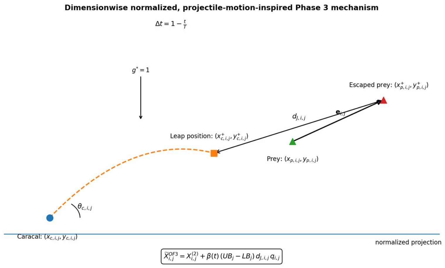
Figure 3 schematically illustrates the dimension-wise normalized and projectile-motion-inspired Phase 3 mechanism, in which the caracal performs a ballistic leap, the prey moves along the normalized escape direction, and the resulting separation is used to generate the range-scaled candidate position.
This normalization prevents the projectile-motion-inspired operator from being directly dominated by the original scale of the decision variables. For each decision variable, the normalized caracal position is projected onto a two-dimensional plane as (Equation (33)):
x c , i , j = X i , j cos ( θ c , i , j ) , y c , i , j = X i , j sin ( θ c , i , j ) ,
and the normalized prey position is projected as (Equation (34)):
x p , i , j = X p r e y , j cos ( θ p , i , j ) , y p , i , j = X p r e y , j sin ( θ p , i , j ) .
These projected coordinates are dimensionless quantities used to construct the search operator. They should not be interpreted as actual physical coordinates measured in meters.
The remaining normalized leap duration and the dimensionless gravitational coefficient are defined as (Equation (35)):
Δ t = 1 t T ,   g = 1 ,
where t and T denote the current and maximum iteration numbers, respectively. The physical value 9.81   m / s 2 is not employed because the decision variables do not generally represent physical position variables measured in consistent units. Instead, g = 1 provides a dimensionless downward-effect term within the normalized movement model.
Based on the conventional horizontal and vertical relations of projectile motion [74,75,76], the projected position of the caracal after the leap is calculated as (Equations (36) and (37)):
x c , i , j + = x c , i , j + v 0 , i cos ( θ c , i , j ) Δ t
y c , i , j + = y c , i , j + v 0 , i sin ( θ c , i , j ) Δ t 1 2 g ( Δ t ) 2 .
Equations (36) and (37) are inspired by the standard mathematical representation of projectile motion [74,75,76]. Nevertheless, they are used here as components of a normalized optimization operator rather than as an exact physical simulation of the caracal’s trajectory.
After determining the projected leap position of the caracal, the relative displacement from the new caracal position to the current prey position is calculated as (Equation (38)):
Δ x i , j = x p , i , j x c , i , j + , Δ y i , j = y p , i , j y c , i , j + , d e , i , j = ( Δ x i , j ) 2 + ( Δ y i , j ) 2 + ε ,
where ε is a small positive numerical constant used to prevent division by zero.
The component-wise escape direction of the prey is then determined by normalizing the relative-displacement vector (Equation (39)):
e x , i , j = Δ x i , j d e , i , j , e y , i , j = Δ y i , j d e , i , j .
In contrast to the previous formulation, an inverse-tangent or rise–run calculation is not required. The escape direction is obtained directly from the relative-position vector. This representation avoids potential division-by-zero and quadrant-ambiguity problems associated with calculating an escape angle using the inverse tangent.
The magnitude of the prey’s escape step is defined as (Equation (40)):
s p , i = E i ( t ) Δ t .
The updated projected prey position is subsequently calculated as (Equation (41)):
x p , i , j + = x p , i , j + s p , i e x , i , j , y p , i , j + = y p , i , j + s p , i e y , i , j .
Accordingly, the prey moves along the direction extending from the projected caracal position toward the current prey position. Since both E i ( t ) and Δ t decrease over the iterations, the magnitude of the modeled escape movement also generally decreases as the optimization process advances.
Following the caracal leap and prey escape, the component-wise projected distance between the predator and the prey is calculated as (Equation (42)):
d J , i , j = ( x c , i , j + x p , i , j + ) 2 + ( y c , i , j + y p , i , j + ) 2 .
Equation (42) is based on the Euclidean-distance concept [77,78]. However, d J , i , j represents the distance in the normalized two-dimensional projection associated with the j th decision variable. It is not the Euclidean distance between two complete D -dimensional candidate solutions. Related distance and relative-position-based search concepts have also been considered in predator–prey-inspired algorithms such as HBA, HHO, and MPA [35,46,53].
An independent stochastic jump-direction coefficient is generated for every decision variable as (Equation (43)):
q i , j = 2 r J , i , j 1 ,   r J , i , j U ( 0 ,   1 ) ,  
where q i , j [ 1 ,   1 ] . The candidate position generated during Phase 3 is then expressed as (Equation (44)):
X ~ i , j O F 3 = X i , j ( 2 ) + β ( t )   S j   d J , i , j   q i , j .
The multiplication by S j maps the dimensionless projected distance back to the numerical range of the corresponding decision variable. Therefore, Equation (44) represents a normalized and range-scaled stochastic position update. Equation (44) does not force the caracal to move directly toward the candidate prey. Instead, the dimensionless predator–prey separation determines the magnitude of the potential displacement, while the independently generated stochastic coefficient determines its direction in each decision dimension. Thus, the operator combines prey-dependent step scaling with stochastic local search. The decreasing coefficient β ( t ) progressively limits the displacement magnitude during the later stages of the optimization process, whereas the greedy selection mechanism prevents an inferior candidate from replacing the current solution.
Before evaluating the objective function, the generated candidate is restricted to the feasible search interval (Equation (45)):
X ^ i , j O F 3 = min [ U B j   , max ( L B j   ,   X ~ i , j O F 3 ) ] .
The objective-function value of the bounded candidate is subsequently calculated as (Equation (46)):
F O i O F 3 = f ( X ^ i O F 3 ) .      
For a minimization problem, the candidate generated in Phase 3 replaces the current solution obtained after Phase 2 when it provides an equal or better objective-function value (Equation (47)):
X i ( 3 ) = { X ^ i O F 3 , F O i O F 3 F O i ( 2 ) , X i ( 2 ) , otherwise .
Here, F O i ( 2 ) = f ( X i ( 2 ) ) , and X i ( 3 ) represents the final position of the i th caracal after the completion of all three phases.
Accordingly, Phase 3 combines the random initial escape-energy structure adapted from HHO [46], the time-dependent coefficient adopted from MPA [53], the projectile-motion relations supported by [74,75,76], and the Euclidean-distance concept [77,78]. The normalization, direct prey-escape direction, dimensionless gravitational effect, and range-scaled stochastic position-update mechanisms constitute the formulation employed in the present ACOA phase. This structure models the essential logic of a leaping predator reacting to escaping prey, but it should not be interpreted as an exact biomechanical or physical simulation of a real Anatolian caracal. Pseudocode of ACOA is presented below in Algorithm 1.
Algorithm 1. Pseudocode of the Anatolian Caracal Optimization Algorithm (ACOA)
Input: Objective function f, problem dimension D, lower and upper bounds LB and UB, population size N, and maximum number of iterations T.
Output: Best objective-function value FObest, best position Xbest, and convergence curve.
1Compute the search range S and the safe normalization range Ssafe using Equations (29) and (30).
2Initialize the population using Equation (1) and construct the population matrix using Equation (2).
3Evaluate the objective-function value of each initial candidate solution using Equation (3).
4Determine the initial best objective-function value FObest and its position Xbest.
5for t = 1 to T do
6  Compute β(t) using Equation (7), set k = 0.2 using Equation (14), and compute β1(t) using Equation (15).
7  Generate the Lévy and Brownian matrices RL and RB for the current iteration using Equations (18) and (19).
8  Randomly select one individual p from the current population as the candidate prey.
9  Store Xprey = Xp and FOprey = FOp; keep both unchanged throughout the current iteration.
10  for i = 1 to N do
11    Phase 1: Wide-area scanning (exploration)
12    Generate independent r1,i, r2,i ~ U(0,1) and randomly select Li ∈ {1,2}.
13    Randomly select m r a n d ≠ i according to Equation (4).
14    if FOprey < FOi then
15        Generate the Phase 1 candidate position using Equation (5).
16    else
17        Generate the Phase 1 candidate position using X m r a n d c u r and Equation (6).
18    end if
19    Restrict the Phase 1 candidate position to the feasible bounds using Equation (8).
20    Evaluate its objective-function value using Equation (9).
21    Apply the greedy selection rule in Equation (10) and immediately write the accepted solution to the current population.
22    Phase 2: Tracking–approach (exploration–exploitation transition)
23    Generate qi ~ U(0,1) and independent ρi,j ~ U(0,1) for j = 1, …, D, as described in Equation (13).
24    if qi < 0.5 then
25        Compute the Lévy-based step using Equation (16).
26        Generate the Phase 2 candidate position using Equation (11).
27    else
28        Compute the Brownian-based step using Equation (17).
29        Generate the Phase 2 candidate position using Equation (12).
30    end if
31    Restrict the Phase 2 candidate position to the feasible bounds using Equation (21).
32    Evaluate its objective-function value using Equation (22).
33    Apply the greedy selection rule in Equation (23) and immediately write the accepted solution to the current population.
34    Phase 3: Predatory leap (exploitation-oriented phase)
35    Generate E0,i, compute Ei(t), and determine the non-negative leap-speed magnitude v0,i using Equations (24)–(26).
36    Generate the caracal and prey movement angles using Equations (27) and (28).
37    Normalize the current caracal position and the fixed prey position using Equations (31) and (32).
38    Project the normalized caracal and prey positions onto the dimension-wise two-dimensional planes using Equations (33) and (34).
39    Compute the remaining normalized leap duration Δt and set g* = 1 using Equation (35).
40    Compute the projected post-leap caracal position using Equations (36) and (37).
41    Compute the relative displacement and de,i,j using Equation (38).
42    Determine the normalized prey-escape direction using Equation (39).
43    Compute the prey-escape step and update the projected prey position using Equations (40) and (41).
44    Compute the projected caracal–prey separation d J , i , j using Equation (42).
45    Generate the independent stochastic jump-direction coefficient qi,j ∈ [−1,1] using Equation (43).
46    Generate the normalized and range-scaled Phase 3 candidate position using Equation (44).
47    Restrict the Phase 3 candidate position to the feasible bounds using Equation (45).
48    Evaluate its objective-function value using Equation (46).
49    Apply the greedy selection rule in Equation (47) and immediately write the accepted solution to the current population.
50  end for
51  Determine the best candidate in the updated population.
52  If the current best solution improves FObest, update FObest and Xbest.
53  Record FObest and the mean population fitness for iteration t.
54end for
55Return FObest, Xbest, and the convergence curve.
Computational and Memory Complexity Analysis
Let N ,     D , and T   denote the population size, problem dimension, and maximum number of iterations, respectively, while C f represents the computational cost of one objective-function evaluation. The initialization of N candidate solutions in a D-dimensional search space requires O ( N D ) operations, whereas evaluating the initial population requires O ( N C f ) .
At each iteration, the generation of the Lévy-flight and Brownian-motion matrices requires O ( 2 N D ) operations. ACOA then applies three sequential search stages to every search agent. Each stage includes D-dimensional position updating, boundary handling, one objective-function evaluation, and greedy selection. Therefore, the three stages require O ( 3 N ( D + C f ) ) operations per iteration. Updating the best-so-far solution additionally requires O(N).
Accordingly, the overall computational complexity of ACOA can be expressed as
O ( N D + N C f + T [ 2 N D + 3 N ( D + C f ) + N ] ) .
After omitting constant factors and lower-order terms, the asymptotic complexity becomes O ( T N ( D + C f ) ) . For benchmark functions whose evaluation cost is proportional to the problem dimension, i.e., C f = O ( D ) , this expression is reduced to O ( T N D ) . It should be noted that the asymptotic notation does not reflect the constant factor associated with the three sequential stages. Therefore, the exact number of objective-function evaluations is also reported as
N F E = N + 3 N T .
The memory requirement is dominated by the population matrix X, the Lévy-flight matrix RL, and the Brownian-motion matrix RB, each of size N × D. The algorithm also stores an N-element fitness vector, a convergence history of length T, the current best solution, and a constant number κ of D-dimensional temporary vectors. Therefore, the peak memory complexity is O ( 3 N D + N + T + κ D + 1 ) , which simplifies to O ( N D + T ) . If the convergence history is not retained, the memory complexity is reduced to O ( N D ) . Although MATLAB may allocate additional temporary arrays during vectorized operations, these arrays do not change the asymptotic memory class.

4. Experimental Results and Discussion

This section presents the simulation and experimental evaluation of ACOA on various benchmark suites, including CEC 2017, CEC 2020, and CEC 2022, as well as engineering design problems, multimodal fixed-dimension, multimodal variable-dimension, unimodal fixed-dimension, and unimodal variable-dimension test problems. In total, ACOA is evaluated on 131 functions, which are detailed in this section. The performance results are analyzed and rigorously compared against several state-of-the-art optimization algorithms. Furthermore, ACOA has also been applied to the electric vehicle (EV) charging station placement problem, demonstrating its potential for real-world engineering and energy management applications.

4.1. Benchmark Test Functions

To test the applicability and efficiency of ACOA, benchmark test functions are utilized. These functions can be grouped as CEC test functions, engineering problems, and multimodal fixed-dimension, multimodal variable-dimension, unimodal fixed-dimension, and unimodal variable-dimension problems.

4.2. Experimental Setup

The proposed ACOA is compared with well-known and recent optimization algorithms, namely the Sine–Cosine Algorithm (SCA) [79], Pelican Optimization Algorithm (POA) [57], Black-winged Kite Algorithm (BKA) [80], Smell Agent Optimization (SAO) [81], Salp Swarm Algorithm (SSA) [82], Dingo Optimization Algorithm (DOA) [83], Gradient-Based Optimizer (GBO) [84], Arithmetic Optimization Algorithm (AOA) [85], Harris Hawks Optimization (HHO) [46], Grey Wolf Optimizer (GWO) [54], and Whale Optimization Algorithm (WOA) [33]. Parameters of the algorithms used for the benchmark functions are presented in Table 1. All algorithms are run with an iteration maximum of 1000.
The algorithms were executed with the default control parameters specified in their original publications, using MATLAB R2019b on a 64-bit Intel Core i5 processor running at 3.20 GHz with 16 GB of RAM.

4.3. Performance Comparison

4.3.1. Evaluation of CEC 2017 Benchmark Test Functions

As presented in Table 2, the CEC 2017 benchmark results present mean values and standard deviation of 30 independent runs. These results indicate that ACOA obtains the best mean performance in 27 of the 29 evaluated functions (F2 excluded), with a tie observed (after rounding) for F3, shared with SSA. F in the table denotes function. A single exception is encountered at F24, where POA yields a marginally lower mean value than ACOA (2.603 × 10³ vs. 2.670 × 10³). Aside from this isolated case, a decisive advantage is maintained by ACOA throughout the CEC 2017 suite.
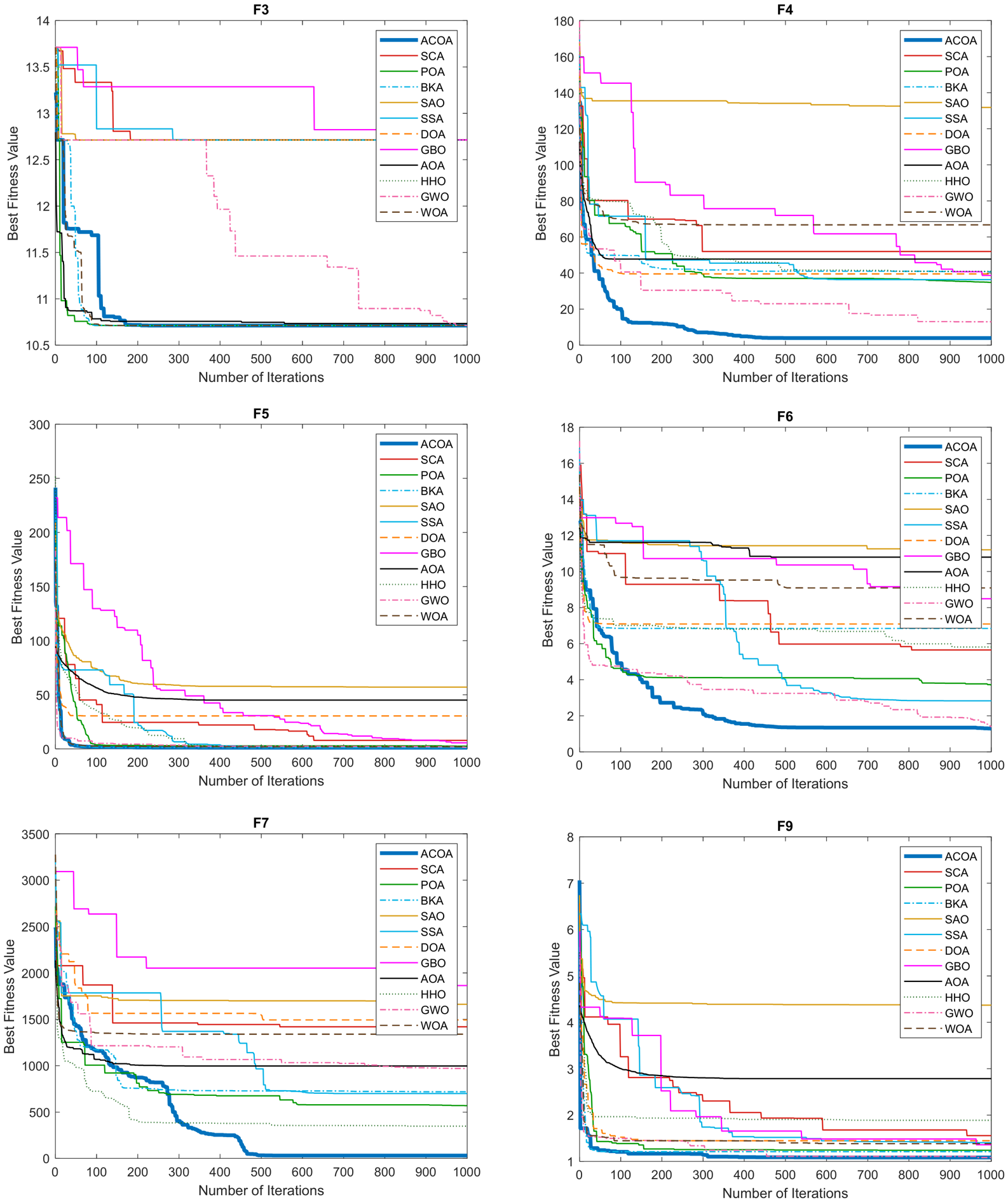
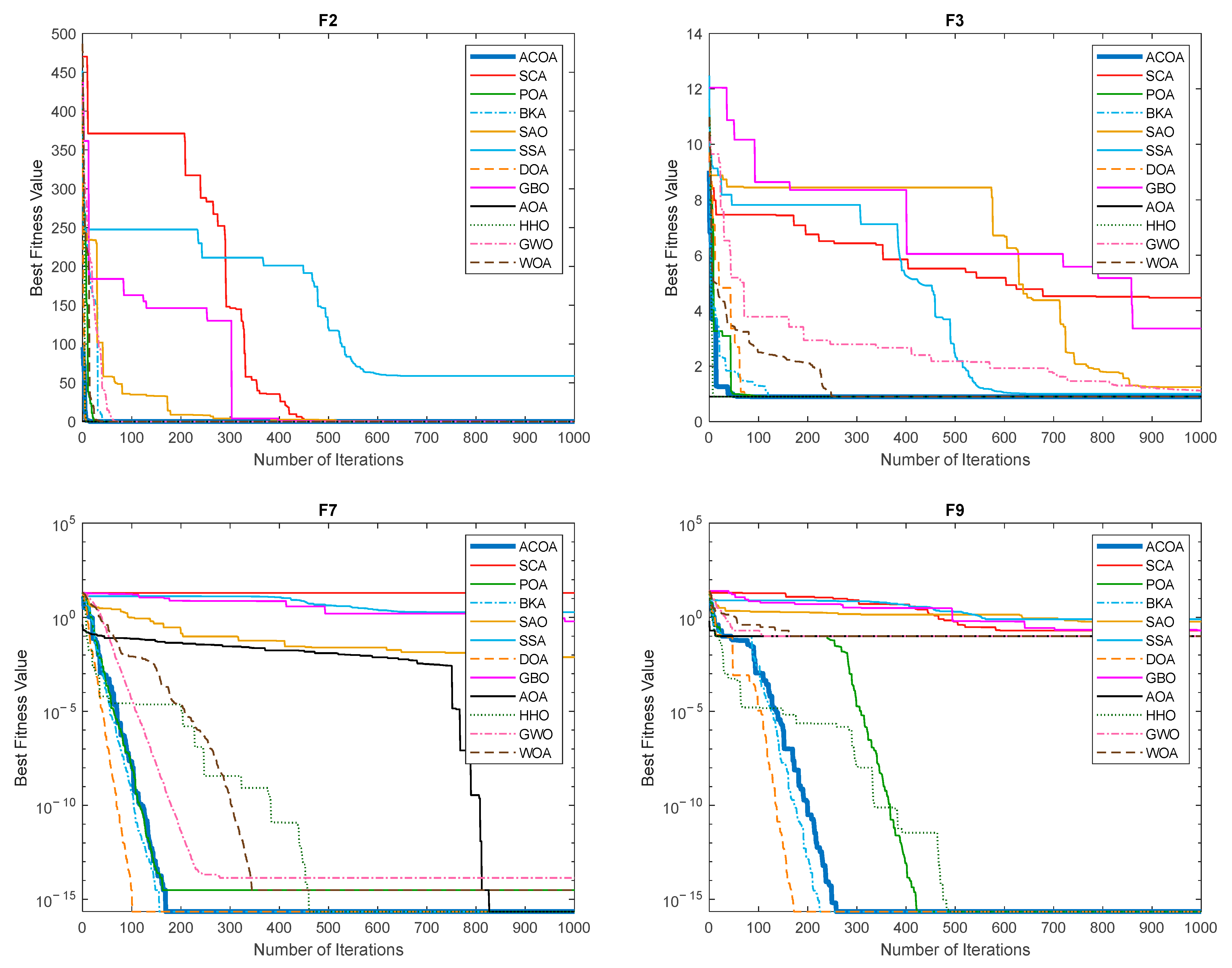
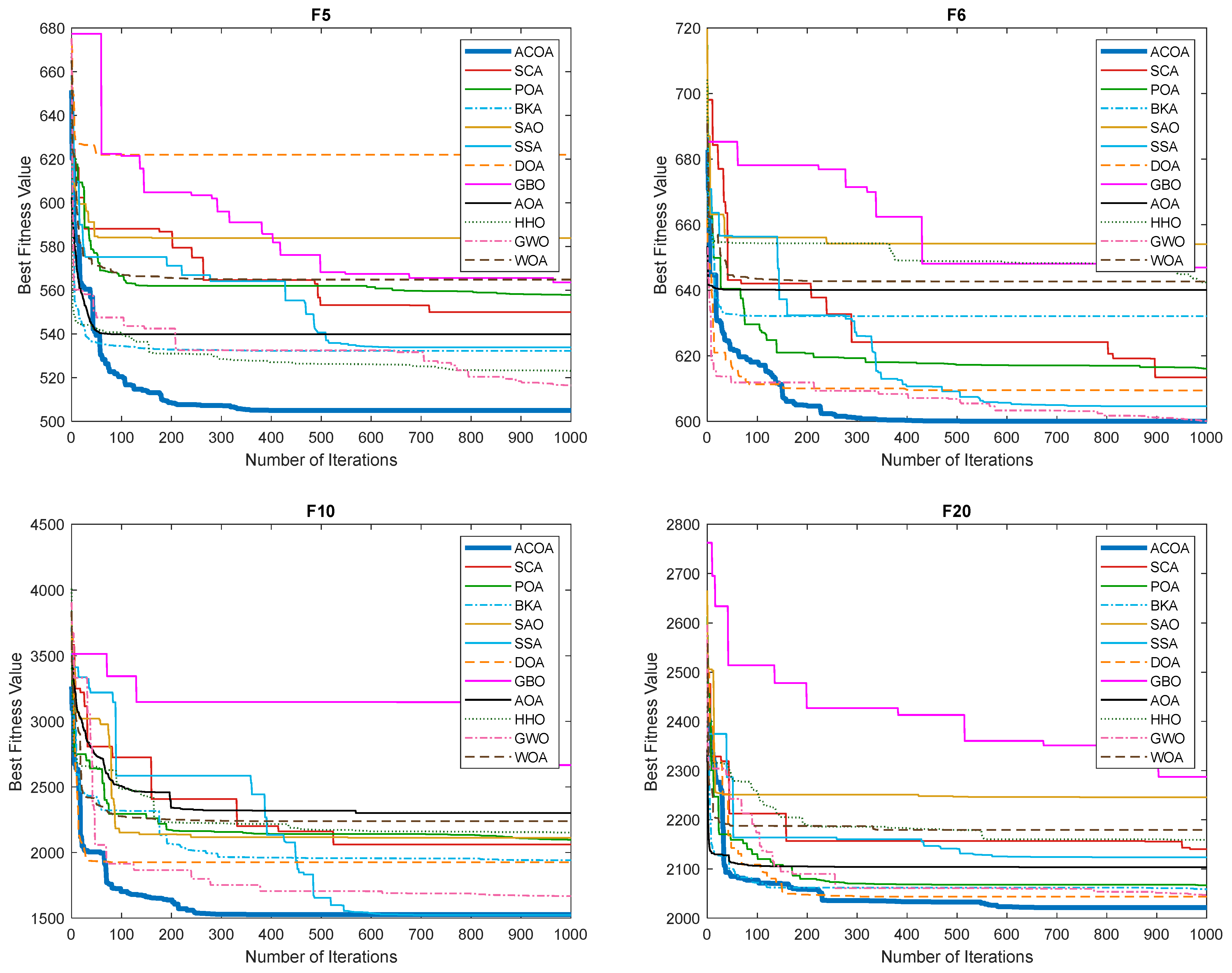
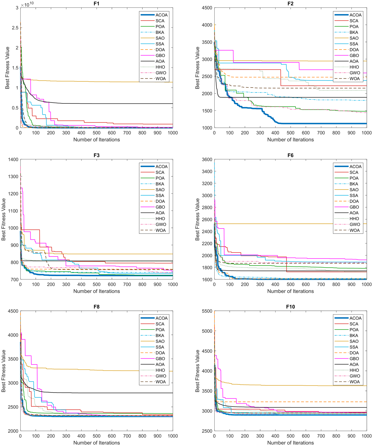
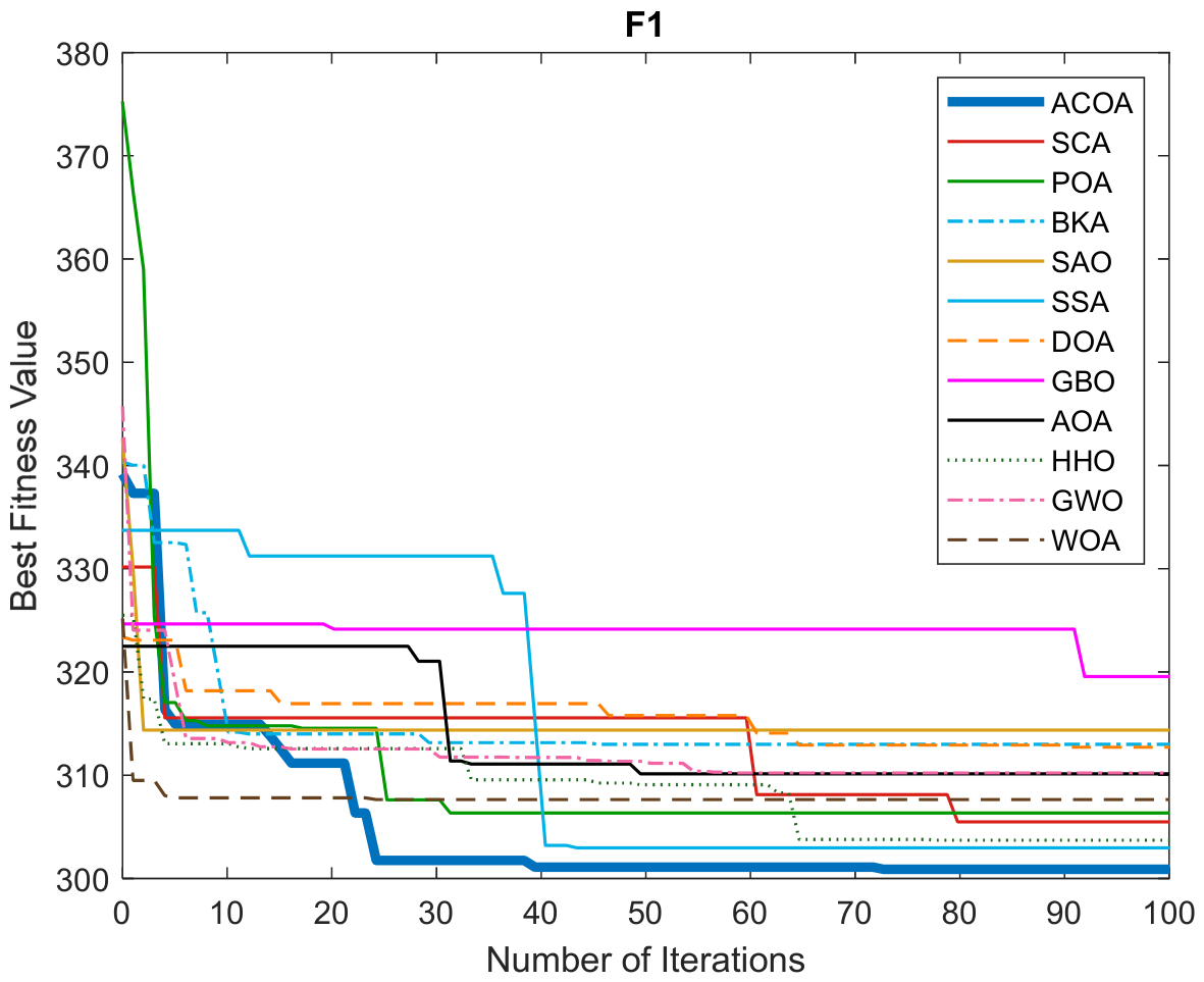
From an exploration–exploitation standpoint, ACOA exhibits strong global search capability in the early stages, effectively exploring a vast solution space, identifying promising regions, and avoiding premature convergence to local optima. The lowest standard deviation is achieved by ACOA across 23 of the 29 CEC 2017 test functions, resulting in lower variance and higher reliability in its solutions, with the exceptions confined to F3, F21, F22, F25, and F26. This result demonstrates that ACOA stands out not only in its average fitness values but also in its statistical stability, reflecting a strong capacity to produce repeatable solutions. This dynamic becomes particularly evident in complex problems. For example, on F30, a mean of 3724 is achieved by ACOA together with a markedly low and stable standard deviation (292.2), in contrast to its competitor, POA, which records a mean of 174,800 and a standard deviation of 382,600, indicating substantially higher variability. Similarly, on F12, while a mean of 2787 is achieved by ACOA against POA’s 69,540—a roughly 25-fold advantage—a smaller standard deviation (2003 vs. 121,300) is also maintained, thereby producing more reliable results compared to its counterparts. On relatively simpler functions such as F4, ACOA’s fine-tuned search capability is evident, consistently delivering low-variance and stable outputs close to the optimum. The convergence curves (Figure 4) further highlight this behavior: rapid improvement in solution quality is observed for ACOA in the early iterations, followed by gradual yet steady progress in the middle and later phases. Convergence curves of several functions exhibited overlapping and visually indistinguishable trajectories. Therefore, only the curves demonstrating separable and readable convergence behavior are included in this study, while highly similar and overlapping curves are omitted for clarity. Collectively, these findings underscore ACOA’s superior balance of exploration and exploitation, yielding both fast early-stage improvements and stable late-stage refinements compared with competing algorithms.
Since F 2 was excluded, the Friedman test was conducted using the mean results obtained for 29 CEC2017 benchmark functions. The test showed a statistically significant difference among the algorithms, with χ 2 ( 11 ) = 233.055 and p = 9.77 × 10 44 . ACOA achieved the lowest mean rank of 1.069 and ranked first among the compared algorithms. In the pairwise Friedman tests, all raw p-values obtained between ACOA and the competing algorithms were below 0.001. These results show that ACOA performed significantly better than all the other algorithms at the α = 0.05 significance level (Table 3).

4.3.2. Evaluation of CEC 2019 Benchmark Test Functions

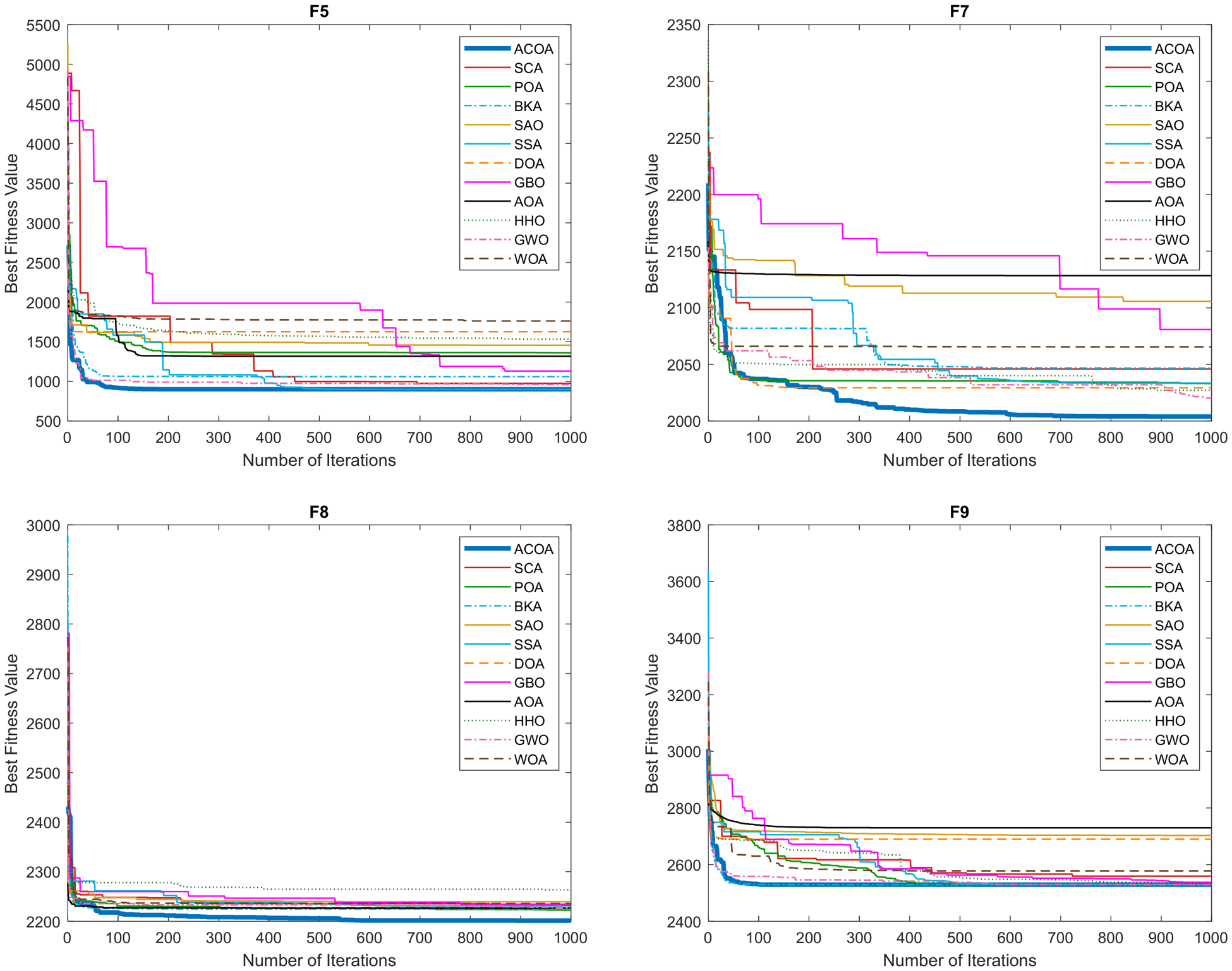
CEC2019 is a challenging benchmark set consisting of shifted/rotated unimodal, multimodal, hybrid, and combination functions for single-objective real-parameter optimization. In this study, the dimensionality of the test functions was determined in accordance with the specific structure of each function. Accordingly, the dimension is set to 9 for the first function, 16 for the second function, and 18 for the third function, whereas a dimension of 10 is adopted for the remaining functions (F4–F10). In this study, the effectiveness of the ACOA algorithm was evaluated over 30 independent runs, and the results are presented in Table 4. According to Table 4, the best mean result is produced by ACOA in nine of the ten functions (F1–F9), with a marginally lower mean obtained by POA only on F10 (19.16 vs. ACOA’s 19.69). In terms of std, the lowest value is produced by ACOA in five functions (F1, F4, F5, F6, and F7). On F10, however, higher variability is observed for ACOA relative to several competitors, where ACOA’s stability is comparatively weakest across the full comparator set. These findings indicate that, while a strong mean-performance advantage is consistently established by ACOA on the CEC2019 test set, its solution consistency is not uniform across all functions, pointing to specific cases where the exploration–exploitation balance could be further refined. The comparatively higher std observed on F10 is consistent with this pattern of increased inter-run scatter on the more difficult functions. Overall, ACOA achieves a good balance between exploration and exploitation on most of the CEC2019 suite, with F10 identified as a function warranting further investigation. Convergence curves for several functions are presented in Figure 5.

4.3.3. Evaluation of CEC 2020 Benchmark Test Functions

The performance of ACOA is compared with other algorithms on 10 independent functions from the CEC 2020 benchmark. According to the results in Table 5, the lowest mean value is achieved by ACOA in nine of the ten test functions, with POA obtaining a marginally lower mean only on F9 (2618 vs. ACOA’s 2666).
For example, on F1, a mean of 2036 is achieved by ACOA, while its closest competitor, SSA, records 3670; the remaining algorithms are separated from ACOA by one to several orders of magnitude (e.g., BKA: 6.238 × 10⁶, POA: 9.912 × 10⁷, SAO: 1.122 × 10¹⁰). On F5, ACOA records 1844, whereas competitors range from 2347 (POA) up to values several orders of magnitude higher (e.g., SAO). Similarly, on F7, ACOA achieves 2131, compared to 2442 (POA), 9603 (SCA), and higher values for the remaining algorithms. ACOA also maintains its advantage in functions where relative differences are narrower: it reaches 2278 on F8 (closest competitors between 2297–2307), and 2915 on F10, essentially matching BKA’s 2921. On F4, where most methods converge on the same mean (≈1900), ACOA’s advantage lies in its stability, evidenced by an extremely low standard deviation (0.26). The single exception within this set is F9, where a marginally lower mean is obtained by POA (2618 vs. ACOA’s 2666), indicating that ACOA’s superiority, while dominant overall, is not absolute across the CEC 2020 suite.
The standard deviation results across 30 independent runs reflecting the balance between exploration and exploitation are generally lower for ACOA, or at least comparable to those of its competitors. For instance, on F3, ACOA demonstrates low volatility (std = 7.97, close to the best competitor’s 9.23); on F4, it achieves a near-zero standard deviation (0.26), reflecting highly consistent results across runs; on F7, it records 32.74, better than competitors. In a few cases, some competitors achieve lower standard deviations. For example, on F9, GBO records 14.83 against ACOA’s 110.3, while on F8, ACOA’s std (38.9) trails SSA’s (23.3). F9 is the function where ACOA’s mean performance is comparatively weakest in this benchmark set. This overall behavior reflects ACOA’s ability to balance diverse exploration in the early stages with stable exploitation in later stages, ensuring consistent improvements. Convergence curves in Figure 6 further confirm this: ACOA diverges early from competitors and steadily increases its lead. For functions like F8 and F10, where differences in mean values are narrower, the curves cluster more closely, yet ACOA sustains a consistent early advantage. Overall, these findings provide quantitative support for ACOA’s effective exploration–exploitation balance, enabling rapid early-stage improvements and stable late-stage refinements, while acknowledging F9 as the one function where a competing algorithm attains a marginally better result.

4.3.4. Evaluation of CEC 2022 Benchmark Test Functions

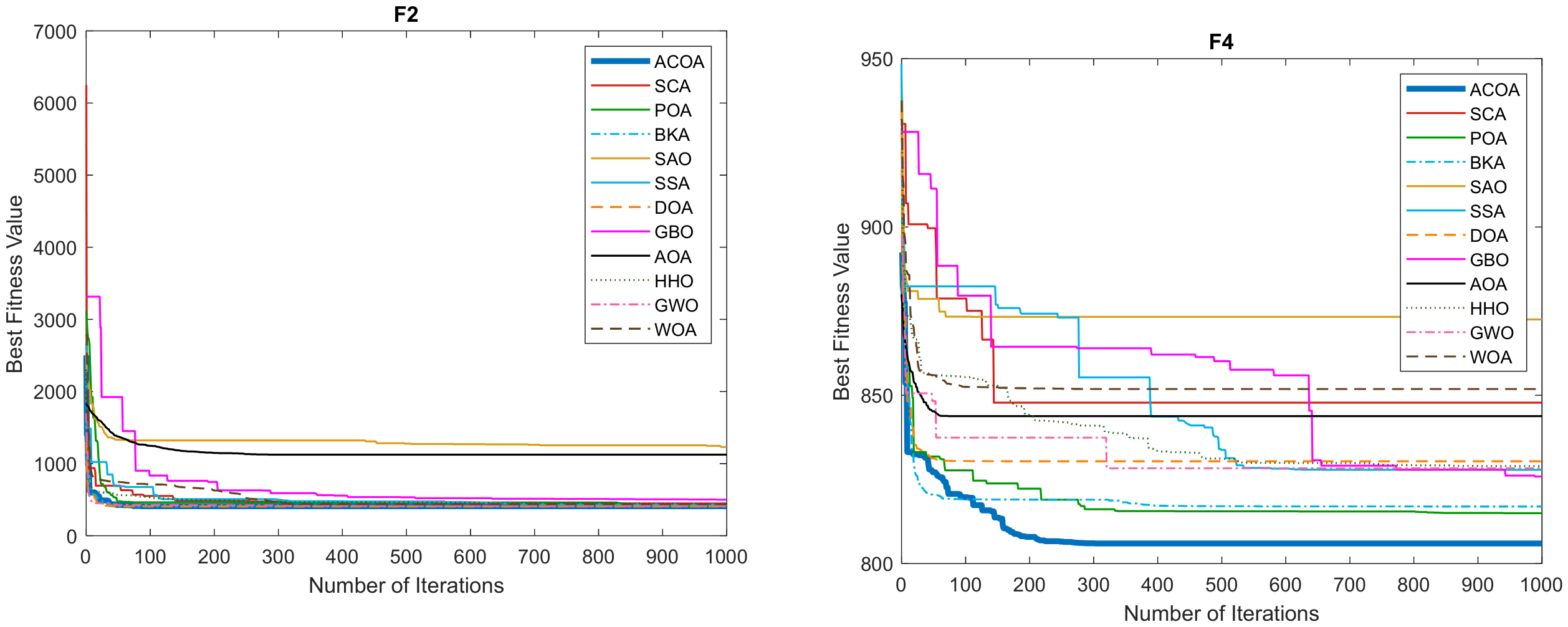
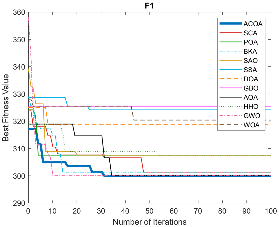
When the CEC 2022 benchmark results are examined (Table 6), it is observed that ACOA achieves the best or equal-to-the-best mean value in eight of the ten functions. The best result is obtained exclusively in F2, F4, F5, F6, F7, F8, F9, and F10, while on F1 a tie/marginal loss to SSA is observed (both at 300 at the reported precision), and on F3 a marginally lower mean is obtained by GWO (600.6 vs. ACOA’s 600.8). In terms of stability, high consistency is demonstrated by ACOA on six functions (F2, F4, F5, F6, F9, and F10), with std values at or below the lowest among 30 independent runs; on F1 and F3, lower std values are obtained by SSA and GWO respectively, and on F7 and F8, lower std values are obtained by SCA. Notably, on F4 (mean = 807.9, std = 3.45) and F5 (mean = 901.3, std = 5.53), as well as on F6 (mean = 1838, std = 19.0) and F9 (mean = 2529, std = 6.775 × 10⁻⁷), both high accuracy and low variance are achieved by the algorithm. The convergence curves in Figure 7 indicate that, for F2, F4, F5, F7, F8, and F9, ACOA reaches the optimum through a rapid decrease in error during the early iterations, maintaining stability with low variance and outperforming its competitors. Furthermore, for F9, equivalent or superior results are achieved in a shorter time, demonstrating a well-balanced integration of exploration and exploitation.

4.3.5. Evaluation of Unimodal Fixed-Dimension Test Functions

Functions in this category are presented in Table 7. Table 8 presents the performance evaluation of the ACOA algorithm, achieving the best results for eight of the nine test functions, with a marginally lower value obtained by AOA only on F4, both values being effectively at machine-precision zero. This demonstrates that ACOA consistently produces optimal or near-optimal solutions across this function set. Furthermore, the observed standard deviation values range from 0 to approximately 6.812 × 10−103, or are very close to zero for all functions. This demonstrates the high consistency of the results across 30 independent runs, confirming the algorithm’s high level of stability. On F1, F2, F3, F4, F6, and F7, near-identical (often exactly equal) results are obtained by multiple compared algorithms, reflecting the relative simplicity of these functions rather than a distinguishing advantage for ACOA. The clearest differentiation is observed on F9 (Colville), where a distinctly lower mean value is achieved by ACOA relative to most competitors, with only four of the twelve algorithms reaching a comparably low result. This highlights the algorithm’s ability to maintain precision on the one function in this set where meaningful separation among algorithms remains possible. These findings confirm that ACOA is a reliable solution method for this class of problems, consistently matching or exceeding the best available result.
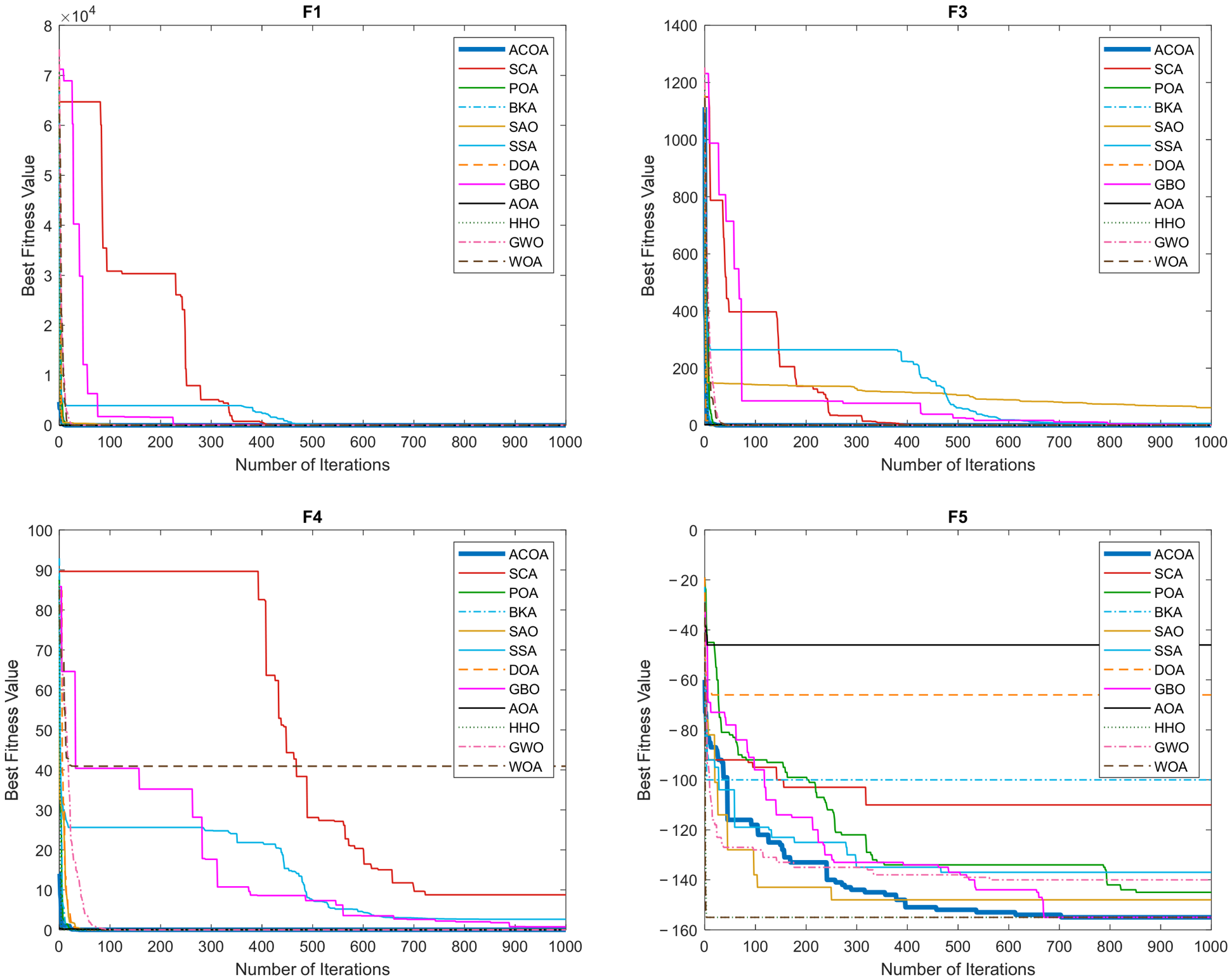
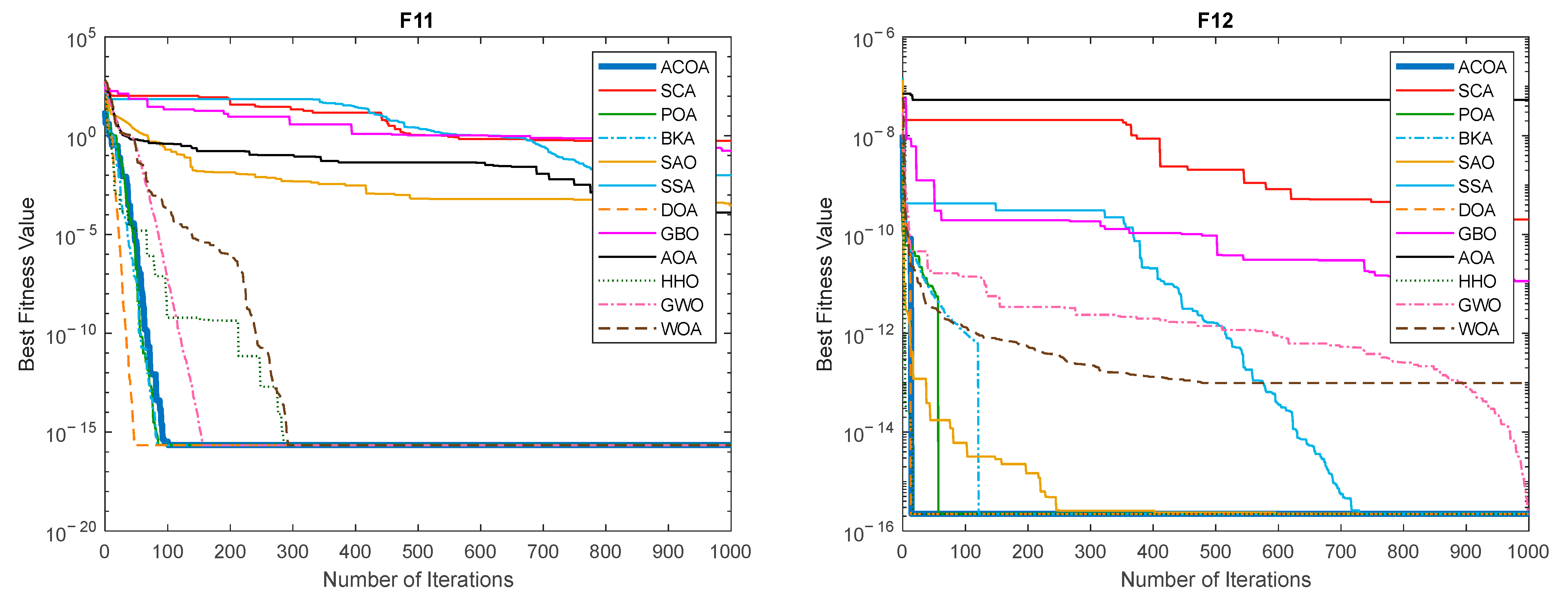
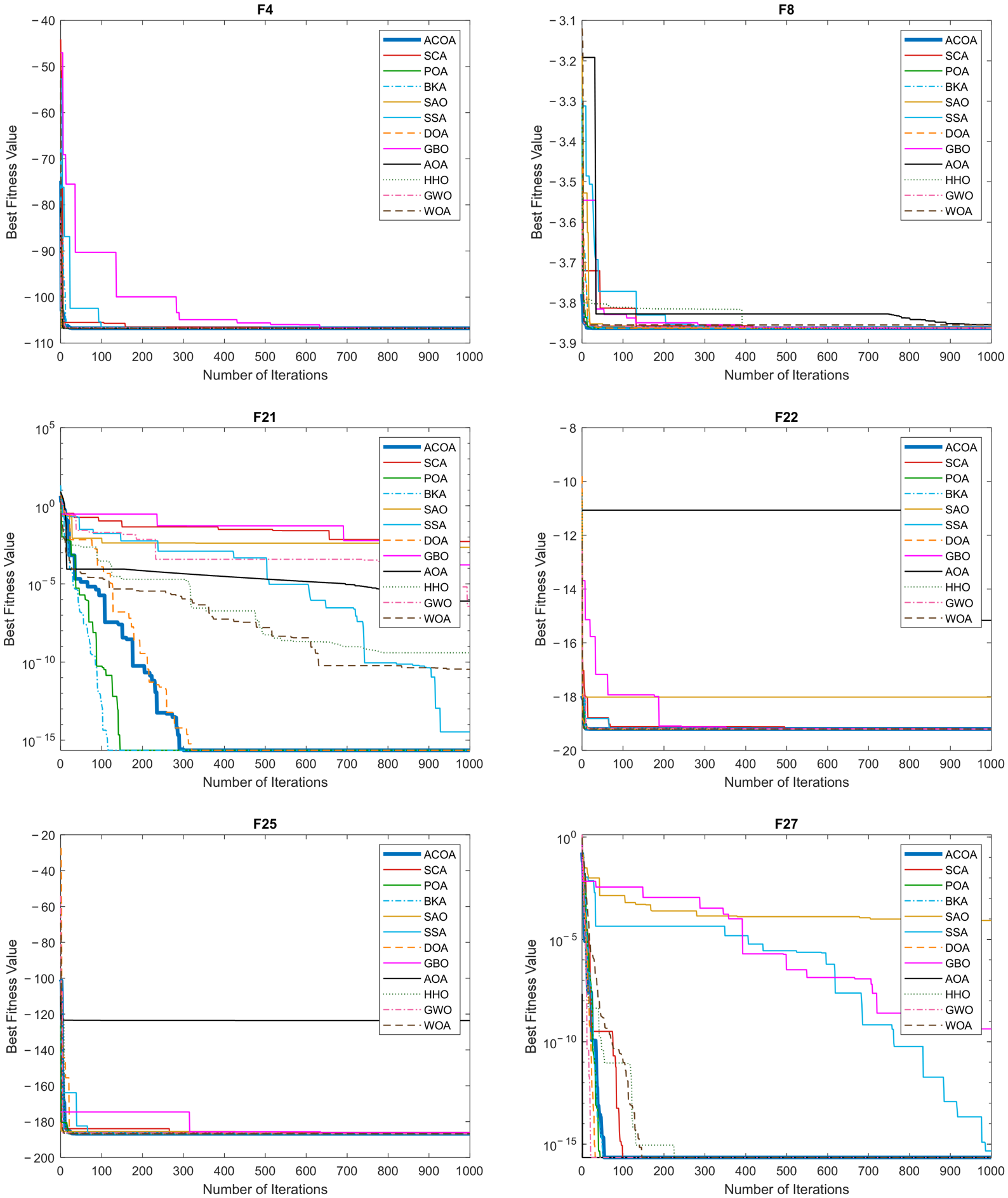
Analysis of the convergence curves for unimodal fixed-dimensional functions (Figure 8) reveals that ACOA exhibits a rapid decline from the first iterations onward for most functions, indicating early convergence toward the optimum. This convergence is both faster and more stable where ACOA achieves the best or most distinctly separated results. For these functions, the curves show a steeper slope in the early iterations, reflecting rapid exploration, before gradually stabilizing in the middle and final iterations as the algorithm transitions to the exploitation phase. Overall, the flatness of the curves indicates that ACOA has reached a stable equilibrium in solution quality, and the low standard deviation values confirm that this stability is consistently replicated across 30 independent runs. These findings demonstrate that ACOA achieves high performance in terms of both speed and stability for unimodal, fixed-dimensional problems, and effectively maintains the exploration–exploitation balance, with F9 offering the clearest evidence of this advantage.

4.3.6. Evaluation of Unimodal Variable-Dimension Test Functions

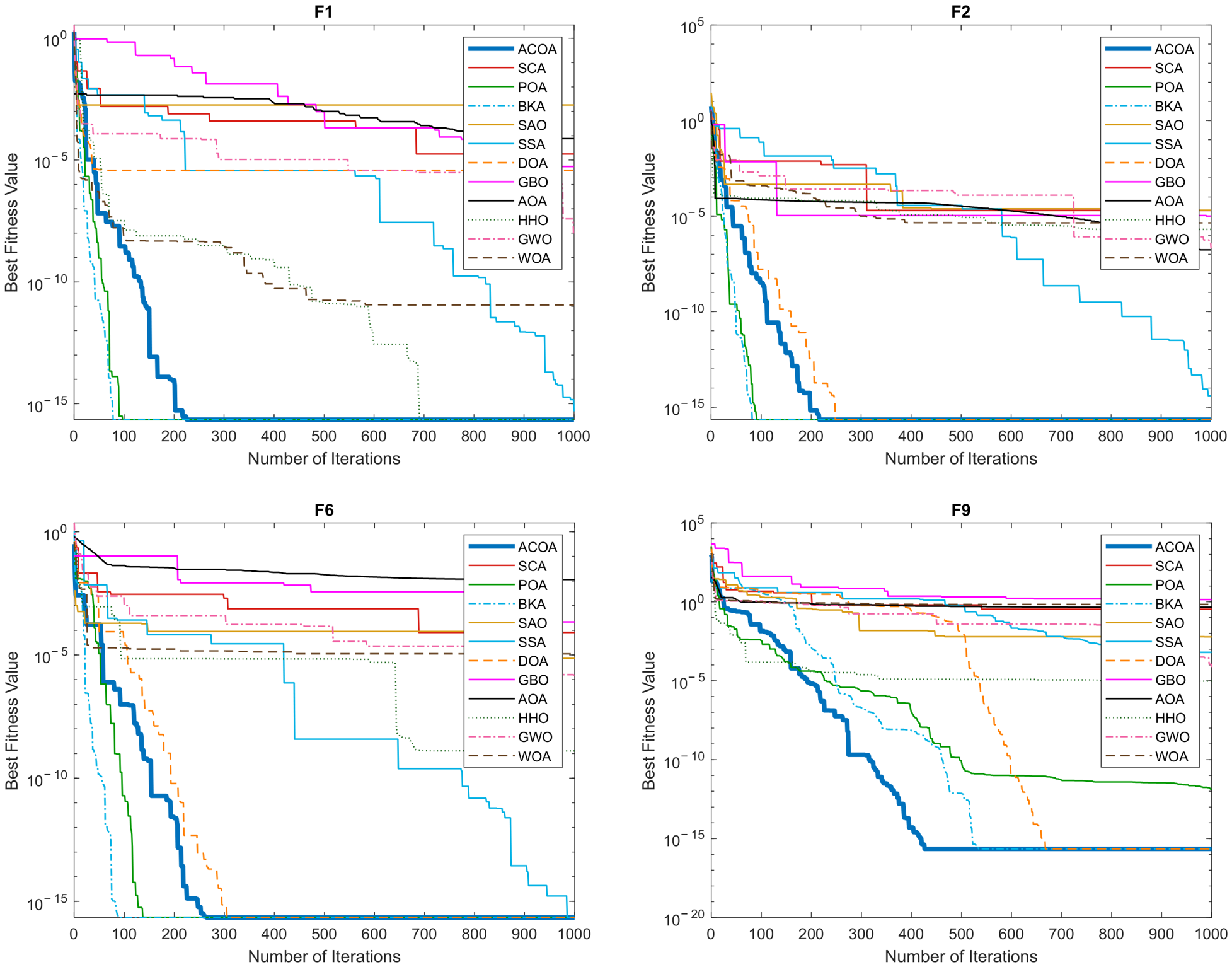
Functions in this category are presented in Table 9. The results presented in Table 10 indicate that ACOA achieved the best solution in 10 of the 12 unimodal variable-dimension test functions. A marginally better mean is obtained by HHO on two functions, Rosenbrock (F8) and Dixon–Price (F10). This demonstrates that ACOA outperforms most of its competitors by delivering high performance on unimodal, variable-dimensional problems, with only a small subset of functions favoring alternative algorithms. An analysis of the mean and standard deviation values over 30 runs shows that ACOA consistently produces very low error values and standard deviations close to zero on the functions where it attains the best result. This indicates that the algorithm not only reaches optimal results but also maintains consistency across different iterations, thereby demonstrating high stability. The low standard deviation values confirm that ACOA effectively balances the exploration and exploitation phases, reaching the optimum without unnecessary oscillations in the solution space. The convergence curves in Figure 9 demonstrate that ACOA rapidly improves from the early iterations on most unimodal functions, reaching the optimal solution faster than competing algorithms. The curves show that the algorithm initially performs extensive exploration of the solution space, then quickly shifts to exploitation to refine the solution. This behavior reduces the time required to reach the global optimum and accelerates convergence on most unimodal problems.

4.3.7. Evaluation of Multimodal Fixed-Dimension Test Functions

Functions in this category are presented in Table 11. The test results presented in Table 12 show that ACOA achieves the best or best-equal mean solution for 21 of the 27 multimodal fixed-dimensional test functions. This corresponds to approximately 78% of the test set, demonstrating the algorithm’s strong performance on functions with high complexity and multiple local optima; the six exceptions (F1, F12, F16, F17, F20, and F27) are functions where AOA, POA, DOA, BKA, or GWO obtain a marginally lower or equal mean. Furthermore, even std analyses clearly demonstrate ACOA’s stability in generating solutions. Specifically, std values of 0 or very close to 0 were obtained for functions F1, F3, F5, F6, F7, F8, F10, F11, F15, F18, F19, F23, F26, and F27. For example, the std value for F1, F23, and F11 is 0, indicating that the same result is produced in all runs; notably, on F26, one of the functions where ACOA also attains the best mean along with BKA, the std (1.8 × 10⁻¹⁵) is lower than that of any competitor. While the std values are higher than those of the competitors on a small number of functions (e.g., F16 and F17), this is generally the result of a more aggressive exploration strategy, which increases solution diversity. Looking at the overall average values, ACOA is among the leading algorithms in terms of stability.
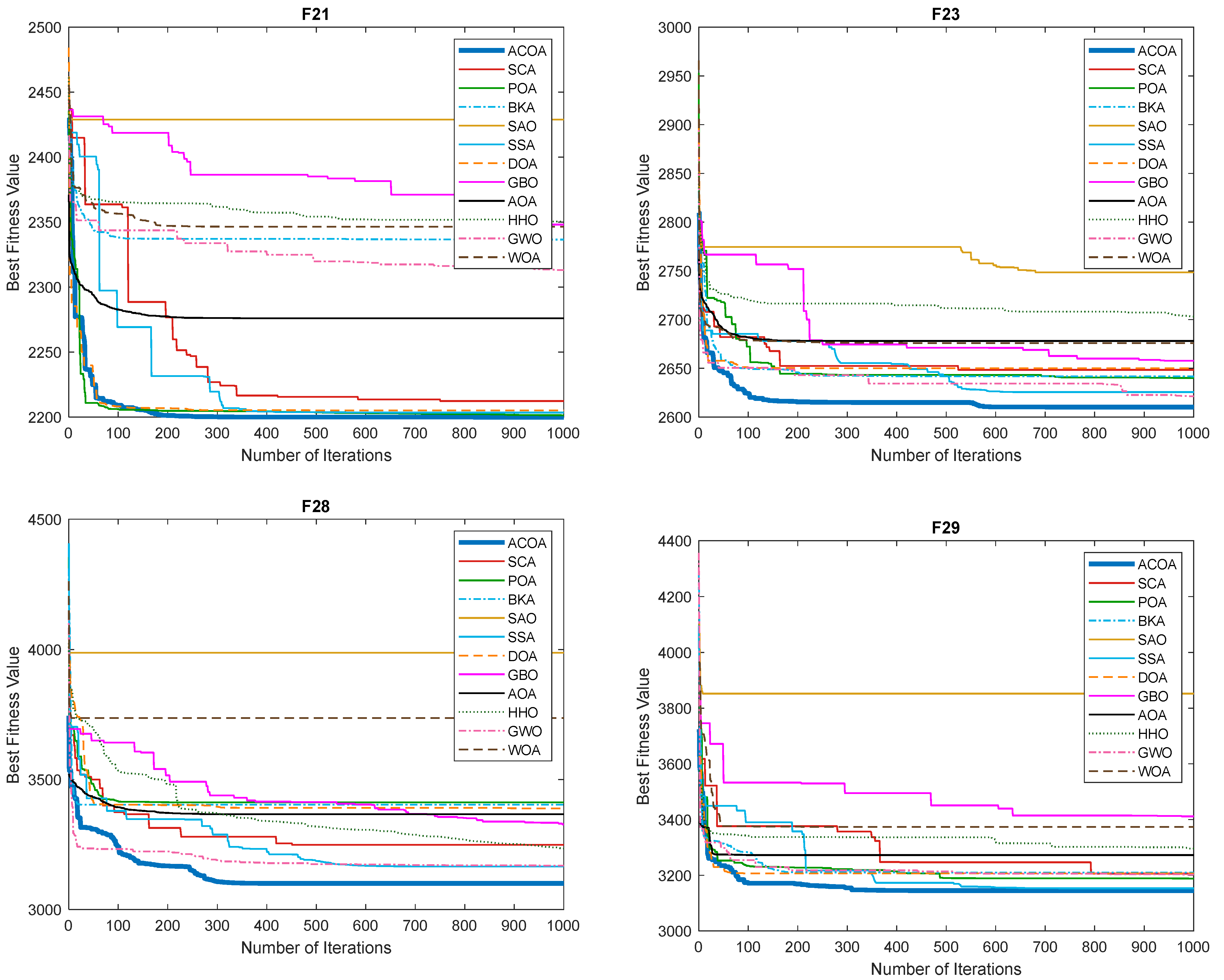
This performance demonstrates ACOA’s ability to manage exploration and exploitation processes in a balanced manner. By scanning a vast solution space in the early stages, ACOA ensures high diversity and minimizes the risk of prematurely getting stuck in local minima. In the middle and late stages, it narrows the solution range, transitions to an intensified exploitation process, and achieves high-accuracy results. This adaptive strategy, particularly the three-stage hunting mechanism, increases the probability of reaching a global optimum in multimodal functions and enhances the reproducibility of results. The convergence curves (Figure 10) clearly reflect ACOA’s iteration-based search strategy. For high-difficulty functions where ACOA attains the best result (e.g., F21), ACOA differentiates itself from its competitors from the very first iterations and gradually increases its advantage. For functions with more minor performance differences, the curves are closely aligned, yet ACOA maintains a slight but decisive advantage until the final iteration. Overall, the results of the multimodal fixed-dimension test functions reveal that ACOA delivers strong and consistent performance in terms of both average success and standard deviation on the large majority of this function set, with the convergence curves visually confirming this behavior. Thanks to its high exploration rate in the early stages and its strategy of stable exploitation in later iterations, ACOA can reliably reach the global optimum while avoiding local minima on most multimodal fixed-dimension problems.

4.3.8. Evaluation of Multimodal Variable-Dimension Test Functions

Functions in this category are presented in Table 13. Table 14 shows the mean and standard deviation results of multimodal variable-dimensional benchmark functions. Among the 16 test functions, the ACOA algorithm obtained the best solution or results equal to the best solution in 11 cases, demonstrating solid performance despite the inherent complexity and robustness of this function set. A marginally better mean is obtained by HHO on four functions (F1, F8, F10, and F14), and by AOA on one function (F6). Compared to other benchmark categories, the multimodal variable-size set remains the area where ACOA’s win rate is comparatively lowest, though the majority of functions are still resolved in its favor. This is expected, as these functions typically contain numerous local optima, making the search more challenging and increasing the risk of premature convergence. From a statistical perspective, the standard deviation values for the functions where ACOA performed well tended to be low, confirming the stability of its solutions across multiple independent runs. This indicates that ACOA effectively balances exploration (extensive search of the solution space) and exploitation (refining solutions in promising areas) for most functions in this set. On the five functions where ACOA falls marginally short of HHO or AOA, higher standard deviation values or slightly lower average scores suggest that its search dynamics could be further refined, potentially through adaptive parameter control, to enhance convergence reliability. Overall, while the multimodal variable-size group remains comparatively more challenging for ACOA than other benchmark categories, its ability to deliver leading results on nearly two-thirds of the functions highlights its robustness and versatility, even in complex search environments.
Analyzing the convergence curves of the multimodal variable-size functions in Figure 11, it is evident that ACOA achieves low error values in a shorter time than most competing algorithms, particularly from the early iterations, with a rapid downward trend. Despite the abundance of local minima in these functions, ACOA effectively employed its extensive exploration capabilities in the early stages and then transitioned to exploitation, steadily improving its solutions. For most functions, the curve shows that ACOA stabilizes in a nearly flat line in regions where competitors are still searching, demonstrating both its high convergence rate and its ability to avoid local minima. In some functions, although other algorithms initially perform faster, ACOA clearly surpasses them in subsequent iterations, achieving lower final error values. This demonstrates that ACOA successfully balances exploration and exploitation on the majority of multimodal, variable-dimensional problems, achieving high solution quality and stability, with a small subset of functions indicating room for further refinement of its late-stage exploitation behavior.
When ACOA was compared with the other algorithms on the multimodal variable-dimension test set, the pairwise Friedman tests showed that ACOA performed significantly better than SCA (p = 6.33 × 10⁻⁵), POA (p = 5.32 × 10⁻⁴), BKA (p = 9.11 × 10⁻⁴), SAO (p = 4.65 × 10⁻⁴), SSA (p = 4.65 × 10⁻⁴), DOA (p = 5.32 × 10⁻⁴), GBO (p = 6.33 × 10⁻⁵), AOA (p = 1.25 × 10⁻²), GWO (p = 6.33 × 10⁻⁵), and WOA (p = 2.01 × 10⁻²) at the α = 0.05 significance level. However, no statistically significant difference was found between ACOA and HHO (p = 3.66 × 10⁻¹). ACOA also achieved the lowest mean rank of 2.375 among the compared algorithms. These results show that ACOA provided better overall performance on the considered test set, while its performance was statistically similar to that of HHO (Table 15).

4.3.9. Constrained Engineering Design Problems

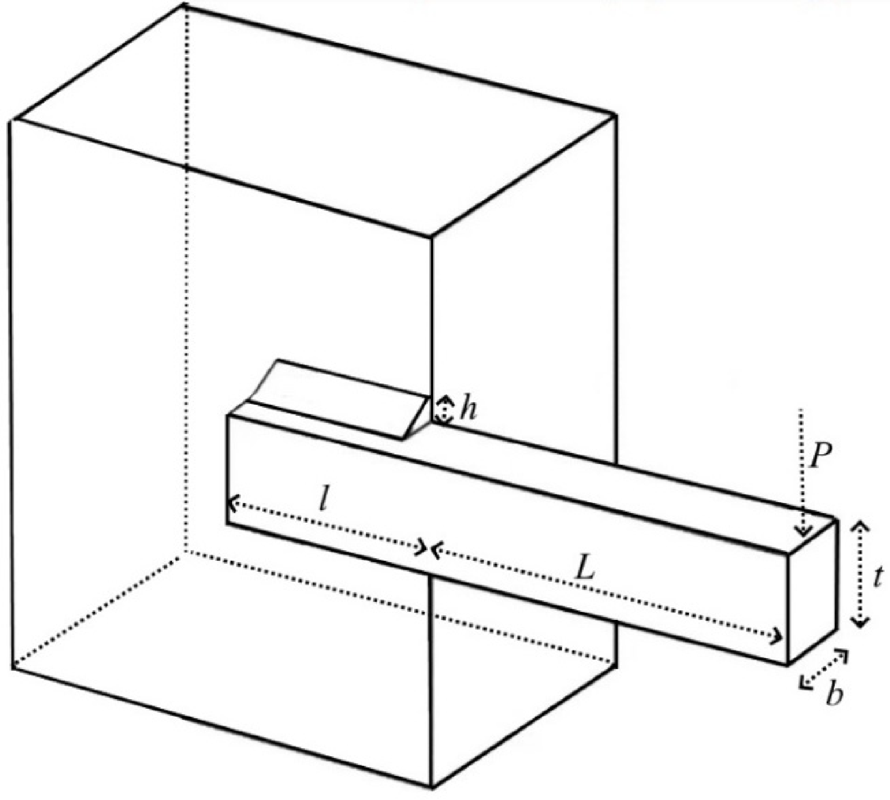
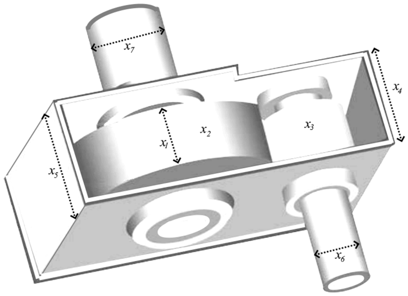
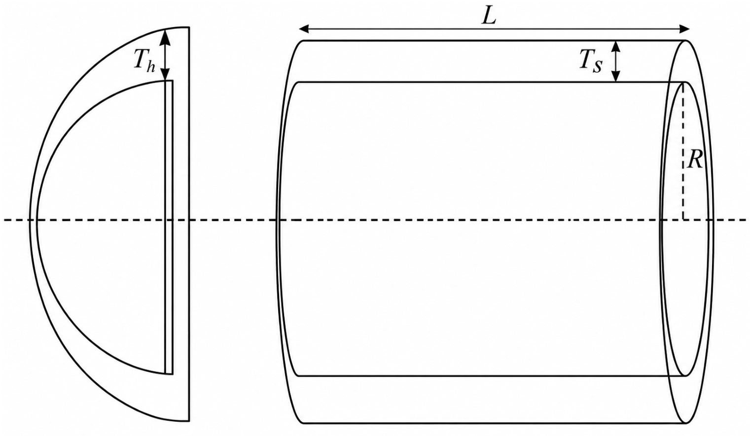
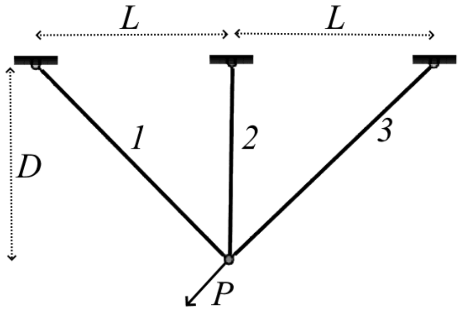
Six real-world restricted engineering problems are used to assess the validity and effectiveness of the suggested ACOA. With multiple design variables and constraints, the problems are highly complicated. Nonetheless, ACOA produced the best outcomes for each of the six engineering problems. The list of engineering design problems with relative parameters is displayed in Table 16.
Tension/Compression Spring Design
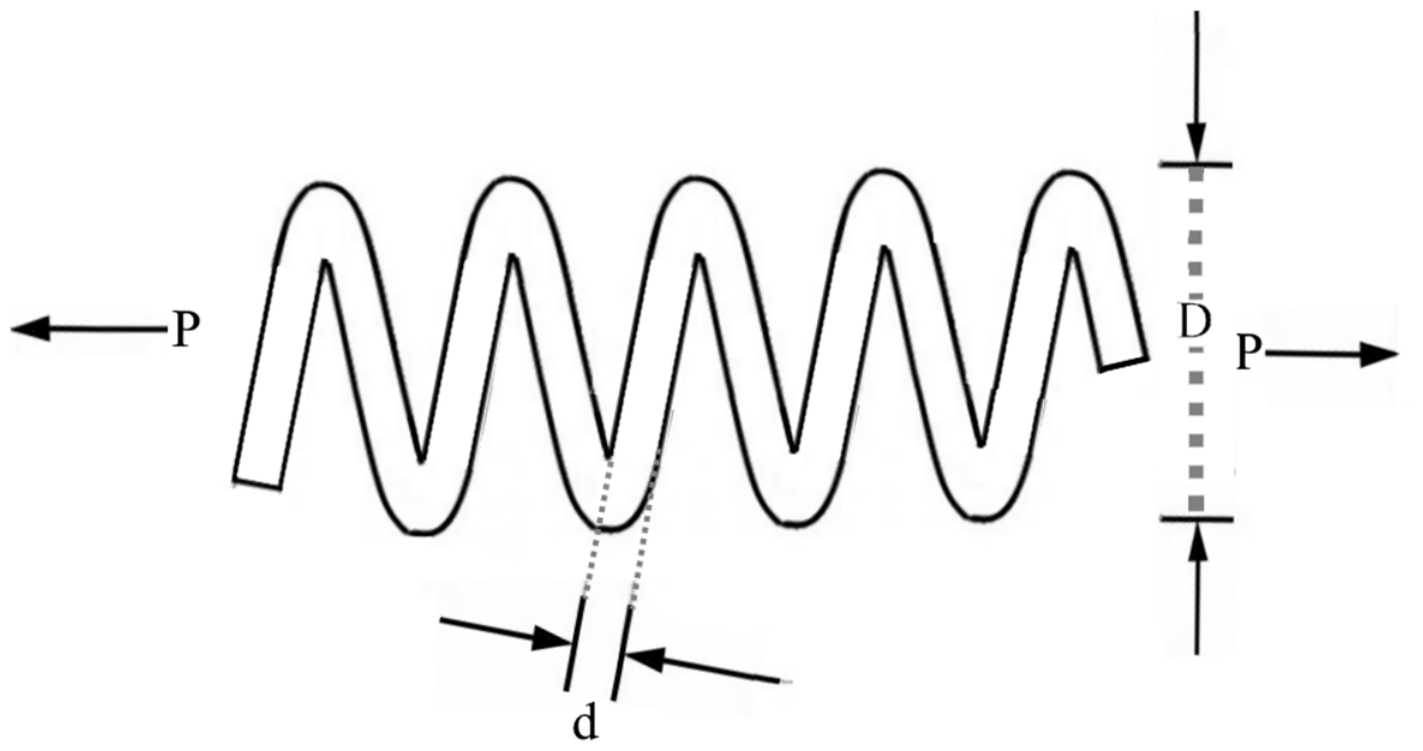
First of the six engineering problems is the tension/compression spring design problem. The goal of this optimization challenge is to reduce the cost of a spring using three different variables. These are coil diameter (D), wire diameter (d), and number of active coils (N). Four constraints are needed to solve the problem: stress, surge frequency, deflection, and diameter boundaries. The illustration of the tension/compression spring design problem is given in Figure 12.
The problem is mathematically formulated as (Equations (50)–(56)):
x = [ x 1 .   x 2 .   x 3 ] = [ d .   D .   N ] ,  
f ( x ) = ( x 3 + 2 ) x 2 x 1 2 .  
Constraints:
g 1 ( x ) = 1 x 2 3 x 3 71785 x 1 4 0 .  
g 2 ( x ) = 4 x 2 2 x 1 x 2 12566 ( x 2 x 1 3 x 1 4 ) + 1 5108 x 1 2 1 0 .
g 3 ( x ) = 1 140.45 x 1 x 2 2 x 3 0 .  
g 4 ( x ) = x 1 + x 2 1.5 1 0 .              
Range of variables:
0.05       x 1   2.00 .     0.25   x 2   1.30 .         2.00       x 3   15.00 .      
According to the results of 30 independent runs on the tension/compression spring engineering problem, the average objective value of ACOA in Table 17 is 1.267 × 10⁻², placing it in the “best” class before rounding. This is matched by POA (1.267 × 10⁻²), with GWO trailing only marginally behind (1.271 × 10⁻²). In contrast, DOA (1.276 × 10⁻²), BKA (1.279 × 10⁻²), SSA (1.287 × 10⁻²), SCA (1.298 × 10⁻²), WOA (1.366 × 10⁻²), GBO (1.374 × 10⁻²), HHO (1.397 × 10⁻²), AOA (1.487 × 10⁻²), and SAO (1.737 × 10⁻²) produced higher (worse) means than ACOA. In terms of stability (std), ACOA is clearly ahead, yielding the lowest standard deviation in the list at 2.69 × 10⁻⁶. This value is roughly one order of magnitude lower than that of its closest competitors, GWO (1.98 × 10⁻⁵) and POA (2.43 × 10⁻⁵), and two to three orders of magnitude lower than the remaining algorithms, ranging up to 5.14 × 10⁻³ (AOA) and 2.50 × 10⁻³ (SAO). This demonstrates that ACOA effectively maintains the exploration–exploitation balance: it enters the correct basin of attraction through sufficient early exploration, then exploits with very low variance, refining the solutions to a consistently tie-best level in a stable and repeatable manner.
Pressure Vessel Design
The aim of the pressure vessel design optimization problem is to minimize the cost of manufacturing a cylindrical pressure vessel. Figure 13 illustrates the design and parameters of the optimization, which include head thickness ( T h ), length of the cylindrical section ( L ) excluding the head, inner radius ( R ), and shell thickness ( T s ).
The mathematical formulation of the problem is (Equations (57)–(63)):
x = [ x 1 .   x 2 .   x 3 .   x 4 ] = [ T s .   T h .   R .   L ] ,                  
f ( x ) = 0.6224 x 1 x 3 x 4   + 1.7781 x 2 x 3 2 + 3.1661 x 1 2 x 4 + 19.84 x 1 2 x 3 .                        
Constraints:
g 1 ( x ) = x 1 + 0.0193 x 3 0 .  
g 2 ( x ) = x 2 + 0.00954 x 3   0 .      
g 3 ( x ) = π x 3 2 x 4 4 3 π x 3 3 + 1296000 0 .
g 4 ( x ) = x 4 240   0 .
Range of variables
0       x 1   99   ,     0   x 2   99   ,             10       x 3   200   ,     10       x 4   200 .          
As presented in Table 18, the results of the pressure vessel design optimization problem demonstrate that the lowest mean value is achieved by ACOA (5898), with POA obtaining the closest competing result (5907) a near-tie in cost outcome, though ACOA retains a marginal but distinct advantage. Regarding standard deviation values, ACOA also achieves the lower variance (33.1) compared to POA (75.1), indicating that ACOA’s consistency is not only competitive but slightly superior to that of its closest rival. Nevertheless, both algorithms clearly outperform the remaining comparators, whose mean values range from 5979 (GWO) up to 7584 (WOA).
Welded Beam Design
The welded beam design problem, seen in Figure 14, is an optimization problem for cost reduction in the manufacturing process. Four decision variables are included in the cost function: the height of the bar (t), the length of the attached part of the bar (l), the weld thickness (h), and the bar thickness (b). Shear stress (s), bucking load on the bar (Pc), and bending stress (θ) are a few of the seven constraints. The problem’s mathematical formulation is:
The problem is formulated as (Equations (64)–(79)):
x = [ x 1 .   x 2 .   x 3 .   x 4 ] = [ h .   l . t .   b ] ,              
f ( x ) = 1.10471 x 1 2 x 2 + 0.04811 x 3 x 4   ( 14 + x 2 ) .                    
Constraints:
g 1 ( x ) = τ ( x ) τ m a x 0 .  
g 2 ( x ) = σ ( x ) σ m a x   0 .  
g 3 ( x ) = x 1 x 4 0 .  
g 4 ( x ) = 0.10471 x 1 2 + 0.04811 x 3 x 4   ( 14 + x 2 ) 5   0 .    
g 5 ( x ) = 0.125 x 1 0 .  
g 6 ( x ) = δ ( x ) δ m a x   0 .    
g 7 ( x ) = P P c ( x ) 0 .  
Range of variables:
0.1       x 1   2 ,               0.1   x 2   10 ,               0.1       x 3   10 ,             0.1       x 4   2 ,
where
M = P ( L + x 2 2 ) ,
R = x 2 2 4 + ( x 1 + x 3 2 ) 2 ,    
J = 2 { 2 x 1 x 2 [ x 2 2 12 + ( x 1 + x 3 2 ) 2 ] } ,    
σ ( x ) = 6 P L x 4 x 3 2 ,
δ ( x ) = 4 P L 3 E x 3 3 x 4 ,    
P c ( x ) = 4.013 E x 3 2 x 4 6 36   L 2   ( 1 x 3 2 L   E 4 G ) .
L = 14 in. δmax = 0.25 in. P = 6000 Lb. E = 30 × 106 psi. G = 12 × 106 psi. τmax = 13,600 psi. σmax = 30,000 psi.
The welded beam design problem is a challenging engineering optimization task aimed at minimizing production costs while satisfying numerous constraints, such as shear stress, bending stress, and buckling load. According to the results of 30 independent runs presented in Table 19, the lowest mean cost is obtained by ACOA before rounding, and POA shares the same result after precision rounding, both converging to 1.725, with GWO closely following at 1.727; the remaining algorithms range up to 2.707 (SAO). The clearest separation among algorithms emerges in terms of stability: ACOA’s standard deviation (4.61 × 10⁻⁸) is markedly lower than that of every competitor, including its closest rival on mean cost, POA, whose standard deviation (3.28 × 10⁻⁵) is roughly three orders of magnitude higher. This confirms that ACOA offers the most efficient performance in balancing exploration and exploitation, with its advantage on this problem expressed primarily through solution consistency, since the mean cost is effectively shared with POA.
Speed Reducer Problem
This engineering design problem aims to select parameters for a speed reducer that minimizes weight for a speed reducer. The problem involves eleven constraints and seven design variables: the face width ( x 1 ), the module of teeth ( x 2 ), the number of teeth on the pinion ( x 3 ), the length of shaft 1 between bearings ( x 4 ), the length of shaft 2 between bearings ( x 5 ), the diameter of the first shaft ( x 6 ), and the diameter of the second shaft ( x 7 ). Figure 15 presents the schematic of the speed reducer design problem.
The problem is formulated as (Equations (80)–(93)):
x = [ x 1 .   x 2 .   x 3 .   x 4 .   x 5 .   x 6 .   x 7 ] ,
f ( x ) = 0.7854 x 1 x 2 2 × ( 3.3333 x 3 2 + 14.9334 x 3 43.0934 ) 1.508 x 1 ( x 6 2 + x 7 2 ) + 7.4777   ( x 6 3 + x 7 3 ) + 0.7854   ( x 4 x 6 2 + x 5 x 7 2 ) .
Constraints:
g 1 ( x ) = 27 x 1 x 2 2   x 3 1 0 .        
g 2 ( x ) = 397.5 x 1 x 2 2   x 3 2 1     0 .    
g 3 ( x ) = 1.93 x 4 3 x 2 x 3 x 6 4 1     0 .  
g 4 ( x ) = 1.93 x 5 3 x 2 x 3 x 7 4 1   0 .
g 5 ( x ) = 1 110 x 6 3 ( 745 x 4 x 2 x 3 ) 2 + 16.9 × 10 6 1 0 .
g 6 ( x ) = 1 85 x 7 3 ( 745 x 5 x 2 x 3 ) 2 + 157.5 × 10 6 1   0 .
g 7 ( x ) = x 2 x 3 40 1 0 .  
g 8 ( x ) = 5 x 2 x 1 1 0 .
g 9 ( x ) = x 1 12 x 2 1 0 .  
g 10 ( x ) = 1.5 x 6 + 1.9 x 4 1 0 .
g 11 ( x ) = 1.1 x 7 + 1.9 x 5 1 0 .  
Range of variables:
  2.6       x 1   3.6   ,       0.7   x 2   0.8   ,         17       x 3   28   ,       7.3       x 4   8.3   ,     7.3   x 5   8.3   ,       2.9       x 6   3.9   ,     5       x 7   5.5 .
The results of 30 independent runs on this challenging engineering problem (speed reducer) are presented in Table 20. According to the findings, ACOA demonstrated the best performance by producing the lowest mean value (2994) and also achieved the lowest standard deviation among all algorithms (0.0218), markedly below even its closest competitor, GWO (3.16). This indicates that ACOA not only delivers accurate results but also provides highly stable solutions. When evaluated in terms of the balance between exploration and exploitation, ACOA shows the most efficient performance by achieving an optimal balance.
Gear Train Design
The gear train design problem is a discrete optimization problem that tries to find the optimum number of tooth for four gears in order to minimize the gear ratio. A schematic of the problem is given in Figure 16, where A, B, C, and D denote the four gears in the train, and the design variables correspond to the number of teeth on each gear (nA, nB, nC, nD). The objective is to minimize the deviation between the actual gear ratio and a desired target ratio, typically expressed as the gear ratio between gears A and D driven through B and C.
Ti represents the number of teeth of the ith gear. The mathematical formulation of this problem is (Equations (94) and (95)):
f ( T a . T b . T c . T d ) = ( 1 6.931 T b × T c T a × T d ) 2 ,
subject to:
12 T a . T b . T c . T d 60 .
The gear train design problem is a discrete optimization task (30 runs) aimed at minimizing the gear ratio by determining the optimal number of teeth for four gears. According to the results presented in Table 21, the ACOA, BKA, HHO, and WOA algorithms achieve the best outcomes by producing a zero-mean value. Moreover, ACOA’s standard deviation is also zero, indicating that it not only reaches the correct solution but does so consistently across all iterations. This highlights the algorithm’s superiority in both accuracy and stability.
Three-Bar Truss Design
The three-bar truss design problem is a classical engineering optimization problem that seeks to minimize the total weight of the truss structure, illustrated in Figure 17, where bars 1, 2, and 3 denote the structural members, L is the horizontal span between the supports, D is the vertical height of the structure, and P is the applied load at the joint. The optimization process is subject to multiple structural constraints, including limits on stress, deflection, and buckling, in order to ensure both safety and mechanical reliability of the system.
The problem is expressed mathematically as follows (Equations (96)–(101)):
x = [ x 1 .   x 2 ] = [ 1 .   2 ] ,
f ( x ) = ( 2 2   x 1 + x 2 ) × L   .      
Constraints:
g 1 ( x ) = 2   x 1 + x 2 2   x 1 2 + 2 x 1 x 2 P σ   0 .      
g 2 ( x ) = x 2 2   x 1 2 + 2 x 1 x 2 P σ     0 .
g 3 ( x ) = 1 2   x 2 + x 1 P σ   0 .  
Range of variables:
0       x 1   1 .     0   x 2   1 ,
where
L = 100   c m .     P = 2   k N c m 2 .     σ = 2   k N c m 2 .
An examination of Table 22 reveals that the ACOA and POA algorithms deliver the best mean value before rounding. POA, BKA, SSA, and GWO achieve the same lowest mean value (263.9) at the reported precision, while DOA, GBO, and HHO (264.0), WOA (264.3), SCA (264.6), AOA (265.0), and SAO (273.0) trail progressively behind. Despite this tie in mean cost among five algorithms, ACOA and POA stand apart in terms of stability, sharing the lowest standard deviation in the comparison at 1.734 × 10⁻¹³, several orders of magnitude lower than the remaining algorithms in this otherwise closely matched set, indicating markedly higher consistency.

4.3.10. Optimal Placement of EVCS in the Distribution Network

EVCS placement is crucial in power systems because unplanned deployment may result in negative consequences such as voltage profile degradation, increased active power losses, sudden load peaks, and overloading of transformers and transmission lines. The solution to this problem is to position EVCSs in the best feasible locations (certain buses) to reduce their impact on the distribution network as much as possible. This placement is based on an index composed of power loss, voltage deviation, and voltage stability index (VSI), which measures a system’s capacity to resume normal operation following a disruption. The results include the locations of EVCSs in the relevant distribution network buses.
Equation (102) presents the multi-objective function formulated for the EVCS placement problem.
m i n {   w 1 × f 1 +   w 2 × f 2 +   w 3 f 3   }   .
The coefficients of the f1, f2, and f3 functions are represented by the weight factors w1, w2, and w3.
The objective function f 1 , which is used to minimize the power loss, is presented in Equation (103):
f 1 = m i n { i = 1 n b r a n c h I i 2   R i } .
The objective function f2, aimed at minimizing voltage deviation, is expressed in Equation (104):
f 2 =   m i n { i = 1 n m a x ( 1   V i )   2   × 100 ×   M V A b } .  
For system stability, it is desirable that the VSI value remains greater than zero; moreover, higher VSI values indicate enhanced stability. The computation of VSI values follows the formulation provided in Ref. [93], while Equation (105) presents the objective function employed for their evaluation:
V S I = m a x { 2 V k 2 V k + 1 2 2 V k + 1 2 ( P k + 1 r   +   Q k + 1 x )     | Z | 2 ( P k + 1 2 + Q k + 1 2 ) } .
In terms of system stability, the weakest link is identified by the minimum VSI value among all calculated VSI values. The lowest VSI value is obtained through Equation (106):
f 3 = m i n { V S I } .
For maintaining optimal power flow, the minimum voltage, power, and voltage stability of the distribution network are constrained within their operational limits, as formulated in Equations (107)–(110):
0 < V S I i           i = 1 .   2 .     .   N ,  
A c t i v e   p o w e r   P i m i n P i P i m a x                 i = 1 .   2 .   N ,  
R e a c t i v e   p o w e r   Q i m i n Q i Q i m a x       i = 1 .   2 .   N ,
B u s   v o l t a g e   V i m i n | V i | V i m a x     i = 1 .   2 .   N ,
where N is the number of buses, P i is active power of i t h bus, Q i is reactive power of i t h bus, and V i is voltage of i t h bus.
The results of the EVCS placement problem for the IEEE3−3 and 69-bus systems are summarized in Table 23 and Table 24, with the convergence profiles of the algorithms shown in Figure 18 and Figure 19. In the IEEE 33-bus system, ACOA achieved the best performance with a mean value of 300.0 and a standard deviation of 5782 × 10−14, producing nearly an identical solution across all 30 independent runs and clearly outperforming other algorithms in terms of stability (e.g., AOA: 0.68, GWO: 3.10, GBO: 10.6), while remaining marginally ahead in mean cost as well (closest competitor: AOA at 300.8). Similarly, in the IEEE 69-bus system, ACOA again achieved the lowest mean value (300.4) together with the lowest variance among all algorithms (std = 0.28). In contrast, the relatively higher standard deviations of other algorithms (e.g., AOA: 2.94, POA: 3.23, GBO: 9.01) highlight ACOA’s superior consistency and stability. The convergence curves in Figure 18 and Figure 19 show that ACOA delivers rapid improvement in the early stages and maintains this trend through the final iterations, exhibiting a more regular and fluctuation-free convergence profile compared to the other algorithms. Overall, these results indicate that ACOA is a powerful and reliable optimization method, distinguished by its accuracy and stability, as well as its effective balance between exploration and exploitation mechanisms in solving the EVCS placement problem.

5. Conclusions

In this study, biological inspiration is derived from the Anatolian caracal, a species distinguished by its superior hunting strategy and remarkable capacity to adapt to harsh environmental conditions. In the context of the large-scale forest fires that have occurred in Türkiye in recent years, this species has demonstrated notable ecological resilience, which provided the motivation for developing a behavior-based optimization approach. Field and literature observations indicate that the caracal’s hunting process consists of three fundamental stages.
  • Wide-Area Scanning (Exploration): The caracal systematically searches a broad region to detect its prey, employing random yet directional movements that maintain diversity in the search process. In the proposed algorithm, this stage is modeled as the global exploration phase, strengthening the capacity to investigate the solution space.
  • Tracking–Approaching (Transition from Exploration to Exploitation): Depending on the type and movement dynamics of the prey, two distinct strategies are observed. For fast-moving targets such as birds, the caracal adopts Lévy-flight-like long jumps, while for relatively static prey such as lizards, it uses Brownian-motion-like small, continuous steps to gradually close the distance. In the algorithm, this stage is modeled through stochastic processes that ensure a smooth and controlled transition from exploration to exploitation.
  • Predatory Leap (Exploitation): Observations reveal that the final strike is executed within a very short time scale, characterized by high acceleration and precise alignment with the target. This process can be explained not only by biological reflexes but also through physical principles. In particular, the relationships among velocity and direction are consistent with classical mechanics and kinematic theories. Consequently, the caracal’s final leap can be likened to the trajectory of a directed body approaching its target. In the algorithm, this stage is modeled as a local intensification mechanism supported by physical formulations, designed to achieve stable convergence to high-quality solutions.
In conclusion, the three-stage hunting strategy of the Anatolian caracal has been integrated with observational evidence and physical principles into a realistic mathematical framework. In this way, a novel optimization algorithm has been developed that is grounded in biological behavior, inspired by nature, and applicable to complex engineering problems. In this respect, the algorithm is built upon the current literature and physics-based correlations. This holistic foundation places the method within a more robust mathematical framework compared to similar studies in the literature, while also serving the goal of more realistically biomimetically replicating the unique hunting characteristics of the Anatolian caracal, thereby distinctly highlighting the method. The algorithm integrates, in a holistic flow, the discovery phase initiated by a wide-area search in the solution space; the transition into exploitation via Brownian and Lévy-based tracking–approach dynamics; and an intensive exploitation phase modeled by predator-leap mechanics through projectile motion physics—thus adaptively maintaining the exploration–exploitation balance.
ACOA has been rigorously compared with SCA, POA, BKA, SAO, SSA, DOA, GBO, AOA, HHO, GWO, and WOA across 131 functions, including fixed-/variable-dimension, single-/multi-modal benchmarks and engineering design problems drawn from the CEC 2017, CEC 2019, CEC 2020, and CEC 2022 competitions. The results demonstrate that ACOA achieved the best or shared-best mean performance on 111 of the 131 functions. Moreover, its performance advantage is more pronounced on the CEC benchmark functions and the various engineering design problems, where ACOA systematically surpasses its competitors in both solution quality and stability.
Moreover, the application of ACOA to the EVCS placement problem demonstrates applicability on standard power-distribution test systems in real-world energy management contexts. The method operates effectively not only on synthetic benchmarks but also under realistic engineering conditions involving constrained resources, network topologies, and demand scenarios. Consequently, the three-stage design of ACOA endows it with rapid and consistent convergence, high solution quality, and statistical robustness qualities that position it as a strong, generalizable, scalable, and practically applicable candidate for both contemporary artificial intelligence applications and engineering optimization tasks.

Author Contributions

Conceptualization, O.A.; methodology, O.A.; software, M.N.; validation, M.N. and T.K.; formal analysis, T.K.; investigation, O.A. and T.K.; resources, O.A. and T.K.; writing—original draft preparation, M.N.; writing—review and editing, O.A.; supervision, O.A.; funding acquisition, M.N. All authors have read and agreed to the published version of the manuscript.

Funding

This research is supported by Inonu University—the Scientific Research Projects (BAP) Unit (No. FBA-2026-5073).

Data Availability Statement

The data presented in this study, including the benchmark evaluation results and the MATLAB implementation of ACOA, are available from the corresponding author upon reasonable request.

Acknowledgments

The authors would like to thank Yasin İlemin from Muğla Sıtkı Koçman University for providing images of the caracal.

Conflicts of Interest

The authors declare that they have no known competing financial interests or personal relationships that could have appeared to influence the work reported in this paper.

References

  1. Al-Baik, O.; Alomari, S.; Alssayed, O.; Gochhait, S.; Leonova, I.; Dutta, U.; Malik, O.P.; Montazeri, Z.; Dehghani, M. Pufferfish Optimization Algorithm: A New Bio-Inspired Metaheuristic Algorithm for Solving Optimization Problems. Biomimetics 2024, 9, 65. [Google Scholar] [CrossRef] [Scilit] [PubMed]
  2. Sergeyev, Y.D.; Kvasov, D.E.; Mukhametzhanov, M.S. On the efficiency of nature-inspired metaheuristics in expensive global optimization with limited budget. Sci. Rep. 2018, 8, 453. [Google Scholar] [CrossRef] [Scilit] [PubMed]
  3. Weng, M. Integer programming. In Logic and Integer Programming; International Series in Operations Research & Management Science; Springer: Boston, MA, USA, 2009; Volume 130. [Google Scholar] [CrossRef] [Scilit]
  4. Burer, S.; Letchford, A.N. Non-convex mixed-integer nonlinear programming: A survey. Surv. Oper. Res. Manag. Sci. 2012, 17, 97–106. [Google Scholar] [CrossRef] [Scilit]
  5. Keller, A.A. Mixed-Integer Nonlinear Programming; Bentham Science Publisher: Sharjah, United Arab Emirates, 2017; pp. 138–172. [Google Scholar] [CrossRef] [Scilit]
  6. El-kenawy, E.S.M.; Khodadadi, N.; Mirjalili, S.; Abdelhamid, A.A.; Eid, M.M.; Ibrahim, A. Greylag Goose Optimization: Nature-inspired optimization algorithm. Expert Syst. Appl. 2024, 238, 122147. [Google Scholar] [CrossRef] [Scilit]
  7. Yildiz, A.R. An effective hybrid immune-hill climbing optimization approach for solving design and manufacturing optimization problems in industry. J. Mater. Process. Technol. 2009, 209, 2773–2780. [Google Scholar] [CrossRef] [Scilit]
  8. Melman, A.; Evsutin, O. Comparative study of metaheuristic optimization algorithms for image steganography based on discrete Fourier transform domain. Appl. Soft Comput. 2023, 132, 109847. [Google Scholar] [CrossRef] [Scilit]
  9. Akdag, O. A Improved Archimedes Optimization Algorithm for multi/single-objective Optimal Power Flow. Electr. Power Syst. Res. 2022, 206, 107796. [Google Scholar] [CrossRef] [Scilit]
  10. Akdag, O.; Yeroglu, C. Optimal directional overcurrent relay coordination using MRFO algorithm: A case study of adaptive protection of the distribution network of the Hatay province of Turkey. Electr. Power Syst. Res. 2021, 192, 106998. [Google Scholar] [CrossRef] [Scilit]
  11. Tikhamarine, Y.; Souag-Gamane, D.; Najah Ahmed, A.; Kisi, O.; El-Shafie, A. Improving artificial intelligence models accuracy for monthly streamflow forecasting using grey Wolf optimization (GWO) algorithm. J. Hydrol. 2020, 582, 124435. [Google Scholar] [CrossRef] [Scilit]
  12. de Albuquerque, V.H.C.; Gupta, D.; De Falco, I.; Sannino, G.; Bouguila, N. Special issue on Bio-inspired optimization techniques for Biomedical Data Analysis: Methods and applications. Appl. Soft Comput. J. 2020, 95, 106672. [Google Scholar] [CrossRef] [Scilit]
  13. Kaveh, A. Applications of Metaheuristic Optimization Algorithms in Civil Engineering; Springer: Cham, Switzerland, 2017. [Google Scholar] [CrossRef] [Scilit]
  14. Ali, H.; Das, S.; Akbar Shaikh, A. Investigate an imperfect green production system considering rework policy via Teaching-Learning-Based Optimizer algorithm. Expert Syst. Appl. 2023, 214, 119143. [Google Scholar] [CrossRef] [Scilit]
  15. Too, J.; Abdullah, A.R. Chaotic Atom Search Optimization for Feature Selection. Arab. J. Sci. Eng. 2020, 45, 6063–6079. [Google Scholar] [CrossRef] [Scilit]
  16. Nurmuhammed, M.; Akdag, O.; Karadag, T. A novel modified Archimedes optimization algorithm for optimal placement of electric vehicle charging stations in distribution networks. Alex. Eng. J. 2023, 84, 81–92. [Google Scholar] [CrossRef] [Scilit]
  17. Abdel-Basset, M.; Mohamed, R.; Azeem, S.A.A.; Jameel, M.; Abouhawwash, M. Kepler optimization algorithm: A new metaheuristic algorithm inspired by Kepler’s laws of planetary motion. Knowl.-Based Syst. 2023, 268, 110454. [Google Scholar] [CrossRef] [Scilit]
  18. Dreo, J.; Petrowsdki, A.; Siarry, P.; Taillard, E.; Chatterjee, A. Metaheuristics for Hard Optimization: Methods and Case Studies; Springer Science & Business Media: New York, NY, USA, 2006. [Google Scholar]
  19. Sivanandam, S.N.; Deepa, S.N. Introduction to Genetic Algorithms; Springer: Berlin/Heidelberg, Germany, 2008. [Google Scholar] [CrossRef] [Scilit]
  20. Bernardino, H.S.; Barbosa, H.J.C. Artificial Immune Systems for Optimization BT—Nature-Inspired Algorithms for Optimisation; Chiong, R., Ed.; Springer: Berlin/Heidelberg, Germany, 2009; pp. 389–411. [Google Scholar] [CrossRef] [Scilit]
  21. Price, K.V.; Storn, R.M.; Lampinen, J.A. The Differential Evolution Algorithm. In Differential Evolution; Springer: Berlin/Heidelberg, Germany, 2006; pp. 37–134. [Google Scholar] [CrossRef] [Scilit] [PubMed]
  22. Montazeri, Z.; Niknam, T.; Aghaei, J.; Malik, O.P.; Dehghani, M.; Dhiman, G. Golf Optimization Algorithm: A New Game-Based Metaheuristic Algorithm and Its Application to Energy Commitment Problem Considering Resilience. Biomimetics 2023, 8, 386. [Google Scholar] [CrossRef] [Scilit] [PubMed]
  23. Givi, H.; Hubálovská, M. Billiards Optimization Algorithm: A New Game-Based Metaheuristic Approach. Comput. Mater. Contin. 2023, 74, 5283–5300. [Google Scholar] [CrossRef] [Scilit]
  24. Dehghani, M.; Montazeri, Z.; Malik, O.P.; Givi, H.; Guerrero, J.M. Shell game optimization: A novel game-based algorithm. Int. J. Intell. Eng. Syst. 2020, 13, 246–255. [Google Scholar] [CrossRef] [Scilit]
  25. Givi, H.; Hubalovska, M. Skill Optimization Algorithm: A New Human-Based Metaheuristic Technique. Comput. Mater. Contin. 2023, 74, 179–202. [Google Scholar] [CrossRef] [Scilit]
  26. Fadakar, E.; Ebrahimi, M. A new metaheuristic football game inspired algorithm. In Proceedings of the 2016 1st Conference on Swarm Intelligence and Evolutionary Computation (CSIEC), Bam, Iran, 9–11 March 2016; pp. 6–11. [Google Scholar] [CrossRef] [Scilit]
  27. Hashim, F.A.; Hussain, K.; Houssein, E.H.; Mabrouk, M.S.; Al-Atabany, W. Archimedes optimization algorithm: A new metaheuristic algorithm for solving optimization problems. Appl. Intell. 2021, 51, 1531–1551. [Google Scholar] [CrossRef] [Scilit]
  28. Koç, İ. Big Bang-Big Crunch Optimization Algorithm for Solving the Uncapacitated Facility Location Problem. Int. J. Intell. Syst. Appl. Eng. 2016, 4, 185–189. Available online: https://dergipark.org.tr/en/download/article-file/237281 (accessed on 14 July 2026). [CrossRef] [Scilit]
  29. Rashedi, E.; Nezamabadi-pour, H.; Saryazdi, S. GSA: A Gravitational Search Algorithm. Inf. Sci. 2009, 179, 2232–2248. [Google Scholar] [CrossRef] [Scilit]
  30. Bouchekara, H.R.E.H. Electrostatic discharge algorithm: A novel nature-inspired optimisation algorithm and its application to worst-case tolerance analysis of an EMC filter. IET Sci. Meas. Technol. 2019, 13, 518–522. [Google Scholar] [CrossRef] [Scilit]
  31. Abedinpourshotorban, H.; Mariyam Shamsuddin, S.; Beheshti, Z.; Jawawi, D.N.A. Electromagnetic field optimization: A physics-inspired metaheuristic optimization algorithm. Swarm Evol. Comput. 2016, 26, 8–22. [Google Scholar] [CrossRef] [Scilit]
  32. Kennedy, J.; Eberhart, R. Particle swarm optimization. In Proceedings of the ICNN’95—International Conference on Neural Networks, Perth, WA, Australia, 27 November–1 December 1995; Volume 4, pp. 1942–1948. [Google Scholar] [CrossRef] [Scilit]
  33. Mirjalili, S.; Lewis, A. The Whale Optimization Algorithm. Adv. Eng. Softw. 2016, 95, 51–67. [Google Scholar] [CrossRef] [Scilit]
  34. Arora, S.; Singh, S. Butterfly optimization algorithm: A novel approach for global optimization. Soft Comput. 2019, 23, 715–734. [Google Scholar] [CrossRef] [Scilit]
  35. Hashim, F.A.; Houssein, E.H.; Hussain, K.; Mabrouk, M.S.; Al-Atabany, W. Honey Badger Algorithm: New metaheuristic algorithm for solving optimization problems. Math. Comput. Simul. 2022, 192, 84–110. [Google Scholar] [CrossRef] [Scilit]
  36. Rajabioun, R. Cuckoo optimization algorithm. Appl. Soft Comput. J. 2011, 11, 5508–5518. [Google Scholar] [CrossRef] [Scilit]
  37. Khishe, M.; Mosavi, M.R. Chimp optimization algorithm. Expert Syst. Appl. 2020, 149, 113338. [Google Scholar] [CrossRef] [Scilit]
  38. Bansal, J.C.; Sharma, H.; Jadon, S.S.; Clerc, M. Spider Monkey Optimization algorithm for numerical optimization. Memetic Comput. 2014, 6, 31–47. [Google Scholar] [CrossRef] [Scilit]
  39. Ghaemi, M.; Feizi-Derakhshi, M.R. Forest optimization algorithm. Expert Syst. Appl. 2014, 41, 6676–6687. [Google Scholar] [CrossRef] [Scilit]
  40. Mirjalili, S.Z.; Mirjalili, S.; Saremi, S.; Faris, H.; Aljarah, I. Grasshopper optimization algorithm for multi-objective optimization problems. Appl. Intell. 2018, 48, 805–820. [Google Scholar] [CrossRef] [Scilit]
  41. Trojovska, E.; Dehghani, M.; Trojovsky, P. Zebra Optimization Algorithm: A New Bio-Inspired Optimization Algorithm for Solving Optimization Algorithm. IEEE Access 2022, 10, 49445–49473. [Google Scholar] [CrossRef] [Scilit]
  42. Jia, H.; Rao, H.; Wen, C.; Mirjalili, S. Crayfish Optimization Algorithm; Springer: Dordrecht, The Netherlands, 2023; Volume 56. [Google Scholar] [CrossRef] [Scilit]
  43. Dehghani, M.; Montazeri, Z.; Trojovská, E.; Trojovský, P. Coati Optimization Algorithm: A new bio-inspired metaheuristic algorithm for solving optimization problems. Knowl.-Based Syst. 2023, 259, 110011. [Google Scholar] [CrossRef] [Scilit]
  44. Ezugwu, A.E.; Agushaka, J.O.; Abualigah, L.; Mirjalili, S.; Gandomi, A.H. Prairie Dog Optimization Algorithm; Springer: London, UK, 2022; Volume 34. [Google Scholar] [CrossRef] [Scilit]
  45. Połap, D.; Woźniak, M. Red fox optimization algorithm. Expert Syst. Appl. 2021, 166, 114107. [Google Scholar] [CrossRef] [Scilit]
  46. Heidari, A.A.; Mirjalili, S.; Faris, H.; Aljarah, I.; Mafarja, M.; Chen, H. Harris hawks optimization: Algorithm and applications. Futur. Gener. Comput. Syst. 2019, 97, 849–872. [Google Scholar] [CrossRef] [Scilit]
  47. MiarNaeimi, F.; Azizyan, G.; Rashki, M. Horse herd optimization algorithm: A nature-inspired algorithm for high-dimensional optimization problems. Knowl.-Based Syst. 2021, 213, 106711. [Google Scholar] [CrossRef] [Scilit]
  48. Amiri, M.H.; Mehrabi Hashjin, N.; Montazeri, M.; Mirjalili, S.; Khodadadi, N. Hippopotamus Optimization Algorithm: A Novel Nature-Inspired Optimization Algorithm; Nature Publishing Group: London, UK, 2024; Volume 14. [Google Scholar] [CrossRef] [Scilit] [PubMed]
  49. Dehghani, M.; Hubalovsky, S.; Trojovsky, P. Tasmanian Devil Optimization: A New Bio-Inspired Optimization Algorithm for Solving Optimization Algorithm. IEEE Access 2022, 10, 19599–19620. [Google Scholar] [CrossRef] [Scilit]
  50. Karaboga, D.; Basturk, B. Artificial Bee Colony (ABC) Optimization Algorithm for Solving Constrained Optimization Problems BT—Foundations of Fuzzy Logic and Soft Computing; Melin, P., Castillo, O., Aguilar, L.T., Kacprzyk, J., Pedrycz, W., Eds.; Springer: Berlin/Heidelberg, Germany, 2007; pp. 789–798. [Google Scholar]
  51. Dehghani, M.; Trojovský, P. Osprey optimization algorithm: A new bio-inspired metaheuristic algorithm for solving engineering optimization problems. Front. Mech. Eng. 2023, 8, 1126450. [Google Scholar] [CrossRef] [Scilit]
  52. Neshat, M.; Sepidnam, G.; Sargolzaei, M. Swallow swarm optimization algorithm: A new method to optimization. Neural Comput. Appl. 2013, 23, 429–454. [Google Scholar] [CrossRef] [Scilit]
  53. Faramarzi, A.; Heidarinejad, M.; Mirjalili, S.; Gandomi, A.H. Marine Predators Algorithm: A nature-inspired metaheuristic. Expert Syst. Appl. 2020, 152, 113377. [Google Scholar] [CrossRef] [Scilit]
  54. Mirjalili, S.; Mirjalili, S.M.; Lewis, A. Grey Wolf Optimizer. Adv. Eng. Softw. 2014, 69, 46–61. [Google Scholar] [CrossRef] [Scilit]
  55. Ahmed, A.M.; Rashid, T.A.; Saeed, S.A.M. Cat Swarm Optimization Algorithm: A Survey and Performance Evaluation. Comput. Intell. Neurosci. 2020, 2020, 4854895. [Google Scholar] [CrossRef] [Scilit] [PubMed]
  56. Yazdani, M.; Jolai, F. Lion Optimization Algorithm (LOA): A nature-inspired metaheuristic algorithm. J. Comput. Des. Eng. 2016, 3, 24–36. [Google Scholar] [CrossRef] [Scilit]
  57. Trojovský, P.; Dehghani, M. Pelican Optimization Algorithm: A Novel Nature-Inspired Algorithm for Engineering Applications. Sensors 2022, 22, 855. [Google Scholar] [CrossRef] [Scilit] [PubMed]
  58. Rao, R.V.; Shah, R. BMR and BWR: Two simple metaphor-free optimization algorithms for solving real-life non-convex constrained and unconstrained problems. arXiv 2024, arXiv:2407.11149. [Google Scholar] [CrossRef] [Scilit]
  59. Rao, R.V.; Davim, J.P. Single, Multi-, and Many-Objective Optimization of Manufacturing Processes Using Two Novel and Efficient Algorithms with Integrated Decision-Making. J. Manuf. Mater. Process. 2025, 9, 249. [Google Scholar] [CrossRef] [Scilit]
  60. Rao, R.V.; Taler, J.; Taler, D.; Lakshmi, J. A Unified Optimization Approach for Heat Transfer Systems Using the BxR and MO-BxR Algorithms. Energies 2026, 19, 34. [Google Scholar] [CrossRef] [Scilit]
  61. Beldar, P.; Rao, R.V. A survey on parameter-less optimization algorithms for engineering applications. Arch. Comput. Methods Eng. 2026. [Google Scholar] [CrossRef] [Scilit]
  62. Wolpert, D.H.; Macready, W.G. No free lunch theorems for optimization. IEEE Trans. Evol. Comput. 1997, 1, 67–82. [Google Scholar] [CrossRef] [Scilit]
  63. Akbaba, B.; Ayaş, Z. Temporal Preference of Eurasian Lynx (Lynx lynx) in a Highland Forest in Northwestern Anatolia in Relation to Other Medium and Large Mammal Species. Mammal Study 2021, 46, 285–295. [Google Scholar] [CrossRef] [Scilit]
  64. İlemin, Y. Mortality Record of Caracal and Habitat Loss for Wildcat, Depending on Catastrophic Wildfires of Year 2021 in Southwestern Turkey. Biol. Bull. 2021, 48, S92–S95. [Google Scholar] [CrossRef] [Scilit]
  65. de Buffon, G.L.L.; Daubenton, L.J.M.; de La Ville de Lacépède, B.G.E.; de Montbéliard, P.G. Histoire naturelle, générale et particulière, avec la description du Cabinet du roy, no. 9. c. In Histoire Naturelle, Générale et Particulière, Avec la Description du Cabinet du Roy; De L’Imprimerie Royale: Paris, France, 1761; Available online: https://books.google.com.tr/books?id=qRQOAAAAQAAJ (accessed on 14 July 2026).
  66. İlemin, Y. Marmaris Ve Köyceğiz Karakulak Caracal caracal (Schreber, 1776) Populasyonunun Bazı Ekolojik Özellikleri. Ph.D. Thesis, Muğla Sıtkı Koçman Üniversitesi, Muğla, Türkiye, 2017. [Google Scholar]
  67. Mengüllüoğlu, D.; Ambarlı, H.; Berger, A.; Hofer, H. Foraging ecology of Eurasian lynx populations in southwest Asia: Conservation implications for a diet specialist. Ecol. Evol. 2018, 8, 9451–9463. [Google Scholar] [CrossRef] [Scilit] [PubMed]
  68. İlemin, Y.; Kaynaş, B.Y.; Yılmaz, T. Evidence on Sympatric Occurrence of Caracal caracal and Lynx lynx in Anatolia. Biol. Bull. 2020, 47, 633–639. [Google Scholar] [CrossRef] [Scilit]
  69. Soyumert, A. Camera-Trapping Two Felid Species: Monitoring Eurasian Lynx (Lynx lynx) and Wildcat (Felis silvestris) Populations in Mixed Temperate Forest Ecosystems. Mammal Study 2020, 45, 41–48. [Google Scholar] [CrossRef] [Scilit]
  70. Zaburdaev, V.; Denisov, S.; Klafter, J. Lévy walks. Rev. Mod. Phys. 2015, 87, 483–530. [Google Scholar] [CrossRef] [Scilit]
  71. Mantegna, R.N. Fast, accurate algorithm for numerical simulation of Lévy stable stochastic processes. Phys. Rev. E 1994, 49, 4677–4683. [Google Scholar] [CrossRef] [Scilit] [PubMed]
  72. Humphries, N.E.; Queiroz, N.; Dyer, J.R.M.; Pade, N.G.; Musyl, M.K.; Schaefer, K.M.; Fuller, D.W.; Brunnschweiler, J.M.; Doyle, T.K.; Houghton, J.D.R.; et al. Environmental context explains Lévy and Brownian movement patterns of marine predators. Nature 2010, 465, 1066–1069. [Google Scholar] [CrossRef] [Scilit] [PubMed]
  73. Einstein, A. Investigations on the Theory of, the Brownian Movement; Dover Publications: Garden City, NY, USA, 1956. [Google Scholar]
  74. Galilei, G. Two New Sciences: Including Centers of Gravity and Force of Percussion; Drake, S., Translator; University of Wisconsin Press: Madison, WI, USA, 1974. [Google Scholar]
  75. “Intro to Physics for Non-Majors,” Atlantic OER. Available online: https://pressbooks.atlanticoer-relatlantique.ca/introcollegephysics/chapter/projectile-motion/ (accessed on 14 July 2026).
  76. Cengiz, A.B. Solving and Visualizing the Mechanical Problems in Physics by Solving and Visualizing the Mechanical Problems in Physics by Computer. Master’s Thesis, Dokuz Eylül University, İzmir, Türkiye, 2020. [Google Scholar]
  77. Liberti, L.; Lavor, C.; Maculan, N.; Mucherino, A. Euclidean distance geometry and applications. SIAM Rev. 2014, 56, 3–69. [Google Scholar] [CrossRef] [Scilit]
  78. “Euclidean Distance,” Geeksforgeeks. Available online: https://www.geeksforgeeks.org/maths/euclidean-distance/ (accessed on 14 July 2026).
  79. Mirjalili, S. SCA: A Sine Cosine Algorithm for solving optimization problems. Knowl.-Based Syst. 2016, 96, 120–133. [Google Scholar] [CrossRef] [Scilit]
  80. Du, C.; Zhang, J.; Fang, J. An innovative complex-valued encoding black-winged kite algorithm for global optimization. Sci. Rep. 2025, 15, 932. [Google Scholar] [CrossRef] [Scilit] [PubMed]
  81. Salawudeen, A.T.; Mu’azu, M.B.; Sha’aban, Y.A.; Adedokun, A.E. A Novel Smell Agent Optimization (SAO): An extensive CEC study and engineering application. Knowl.-Based Syst. 2021, 232, 107486. [Google Scholar] [CrossRef] [Scilit]
  82. Mirjalili, S.; Gandomi, A.H.; Mirjalili, S.Z.; Saremi, S.; Faris, H.; Mirjalili, S.M. Salp Swarm Algorithm: A bio-inspired optimizer for engineering design problems. Adv. Eng. Softw. 2017, 114, 163–191. [Google Scholar] [CrossRef] [Scilit]
  83. Peraza-Vázquez, H.; Peña-Delgado, A.F.; Echavarría-Castillo, G.; Morales-Cepeda, A.B.; Velasco-Álvarez, J.; Ruiz-Perez, F. A Bio-Inspired Method for Engineering Design Optimization Inspired by Dingoes Hunting Strategies. Math. Probl. Eng. 2021, 2021, 9107547. [Google Scholar] [CrossRef] [Scilit]
  84. Ahmadianfar, I.; Bozorg-Haddad, O.; Chu, X. Gradient-based optimizer: A new metaheuristic optimization algorithm. Inf. Sci. 2020, 540, 131–159. [Google Scholar] [CrossRef] [Scilit]
  85. Abualigah, L.; Diabat, A.; Mirjalili, S.; Abd Elaziz, M.; Gandomi, A.H. The Arithmetic Optimization Algorithm. Comput. Methods Appl. Mech. Eng. 2021, 376, 113609. [Google Scholar] [CrossRef] [Scilit]
  86. Arora, J.S. Introduction to Optimum Design; McGraw-Hill: New York, NY, USA, 1989. [Google Scholar]
  87. Belegundu, A.D.; Arora, J.S. A Study of Mathematical Programming Methods for Structural Optimization. Part I: Theory. Int. J. Numer. Methods Eng. 1985, 21, 1583–1599. [Google Scholar] [CrossRef] [Scilit]
  88. Kannan, B.K.; Kramer, S.N. An augmented Lagrange multiplier based method for mixed integer discrete continuous optimization and its applications to mechanical design. J. Mech. Des. Trans. ASME 1994, 116, 405–411. [Google Scholar] [CrossRef] [Scilit]
  89. Rao, S.S. Engineering Optimization, 3rd ed.; Wiley: Hoboken, NJ, USA, 1996. [Google Scholar]
  90. Sandgren, E. Nonlinear integer and discrete programming in mechanical design optimization. ASME J. Mech. Des. 1990, 112, 223–229. [Google Scholar] [CrossRef] [Scilit]
  91. Golabi, S.; Fesharaki, J.J.; Yazdipoor, M. Gear train optimization based on minimum volume/weight design. Mech. Mach. Theory 2014, 73, 197–217. [Google Scholar] [CrossRef] [Scilit]
  92. Ray, T.; Saini, P. Engineering design optimization using a swarm with an intelligent information sharing among individuals. Eng. Optim. 2001, 33, 735–748. [Google Scholar] [CrossRef] [Scilit]
  93. Deb, S.; Tammi, K.; Kalita, K.; Mahanta, P. Impact of electric vehicle charging station load on distribution network. Energies 2018, 11, 178. [Google Scholar] [CrossRef] [Scilit]
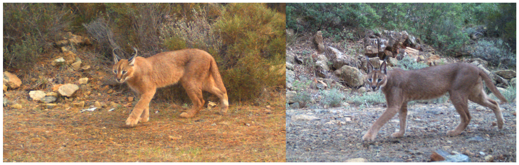
Figure 1. Images of the Anatolian caracal.
Mathematics 14 03007 g001
Figure 2. Three-stage hunting strategy of the Anatolian caracal.
Mathematics 14 03007 g002
Figure 3. Dimension-wise normalized projectile-motion-inspired representation of the Anatolian caracal leap and prey-escape mechanism employed in Phase 3.
Mathematics 14 03007 g003
Figure 4. Convergence curves of ACOA and the comparator algorithms on the first subset of the CEC 2017 benchmark functions (D = 10), showing best-so-far fitness versus iteration number.
Mathematics 14 03007 g004aMathematics 14 03007 g004b
Figure 5. Convergence curves of CEC 2019 benchmark functions.
Mathematics 14 03007 g005
Figure 6. Convergence curves of ACOA and the comparator algorithms on the remaining subset of the CEC 2020 benchmark functions, showing best-so-far fitness versus iteration number.
Mathematics 14 03007 g006
Figure 7. Convergence curves of CEC 2022 benchmark functions.
Mathematics 14 03007 g007aMathematics 14 03007 g007b
Figure 8. Convergence curves of unimodal fixed-dimension functions.
Mathematics 14 03007 g008
Figure 9. Convergence curves of unimodal variable-dimension functions.
Mathematics 14 03007 g009
Figure 10. Convergence curves of multimodal fixed-dimension functions.
Mathematics 14 03007 g010
Figure 11. Convergence curves of multimodal variable-dimension functions.
Mathematics 14 03007 g011aMathematics 14 03007 g011b
Figure 12. Tension/compression spring design.
Mathematics 14 03007 g012
Figure 13. Pressure vessel design problem.
Mathematics 14 03007 g013
Figure 14. Schematic of welded beam design problem.
Mathematics 14 03007 g014
Figure 15. Schematic of speed reducer design problem.
Mathematics 14 03007 g015
Figure 16. Schematic of gear train design problem.
Mathematics 14 03007 g016
Figure 17. Schematic of three-bar truss design problem.
Mathematics 14 03007 g017
Figure 18. Convergence curves of EVCS placement problem for 33 bus.
Mathematics 14 03007 g018
Figure 19. Convergence curves of EVCS placement problem for 69 bus.
Mathematics 14 03007 g019
Table 1. Parameter settings of ACOA and the comparative optimization algorithms for benchmark functions.
AlgorithmParameters
ACOASearch Agents = 50
Beta(t) = (1 − t/T)^(2t/T) [adaptive, no free parameter]
SCA [79]Search Agents = 50; a = 2;
POA [57]Materials_no = 50
BKA [80]Pop = 50; p = 0.9
SAO [81]Molecules = 50; olf = 0.9;
K = 0.6; T = 0.95; M = 0.9; Step = 0.02;
SSA [82]SearchAgents_no = 50
DOA [83]SearchAgents_no = 50
GBO [84]Vector size = 50
AOA [85]Alpha = 5; Mu = 0.499;
HHO [46]SearchAgents_no = 50
GWO [54]SearchAgents_no = 50; a = [2, 0]
WOA [33]SearchAgents_no = 50
Table 2. Evaluation results of best solutions for 30 independent runs on CEC 2017 benchmark test functions (dim = 10).
F ACOASCAPOABKASAOSSADOAGBOAOAHHOGWOWOA
1Mean3.060E+037.079E+084.437E+071.295E+081.129E+103.469E+036.502E+088.508E+075.202E+093.444E+053.863E+073.110E+06
Std3.005E+032.573E+081.268E+082.737E+084.190E+093.937E+031.553E+097.603E+072.864E+091.668E+051.055E+086.609E+06
3Mean3.000E+021.623E+034.630E+027.752E+021.070E+043.000E+021.860E+035.633E+030.000E+003.018E+021.443E+032.450E+03
Std4.808E−059.112E+024.226E+021.694E+033.547E+037.045E−102.436E+032.181E+030.000E+001.137E+001.701E+032.669E+03
4Mean4.001E+024.466E+024.109E+024.020E+021.348E+034.047E+024.742E+024.378E+027.420E+034.085E+024.147E+024.386E+02
Std1.403E−011.259E+011.784E+015.205E+004.602E+021.649E+008.550E+012.930E+012.542E+031.356E+011.569E+013.936E+01
5Mean5.078E+025.479E+025.397E+025.312E+026.042E+025.190E+025.358E+025.439E+026.493E+025.511E+025.168E+025.595E+02
Std2.835E+004.587E+001.377E+011.432E+012.233E+015.466E+001.688E+019.766E+001.756E+021.300E+011.039E+011.840E+01
6Mean6.003E+026.178E+026.162E+026.227E+026.537E+026.090E+026.227E+026.195E+025.528E+026.306E+026.008E+026.350E+02
Std6.273E−013.442E+001.090E+018.082E+001.258E+017.138E+001.194E+018.372E+001.830E+011.056E+011.228E+001.143E+01
7Mean7.214E+027.736E+027.638E+027.477E+028.447E+027.380E+027.569E+027.702E+026.360E+027.836E+027.316E+027.738E+02
Std4.189E+009.207E+001.835E+011.564E+012.242E+011.404E+012.317E+011.514E+017.398E+001.809E+011.077E+012.075E+01
8Mean8.094E+028.406E+028.210E+028.186E+028.699E+028.248E+028.280E+028.373E+027.938E+028.282E+028.128E+028.414E+02
Std3.985E+006.210E+006.904E+007.108E+001.275E+011.175E+011.224E+019.209E+001.531E+017.610E+004.993E+001.907E+01
9Mean9.000E+021.008E+031.052E+031.075E+031.784E+039.538E+021.068E+031.121E+038.276E+021.378E+039.096E+021.423E+03
Std8.491E−026.634E+011.308E+021.261E+023.486E+021.396E+021.549E+022.410E+026.093E+002.307E+021.875E+013.221E+02
10Mean1.398E+032.318E+031.621E+031.716E+032.814E+031.831E+032.338E+032.486E+031.401E+032.096E+031.647E+032.037E+03
Std1.639E+022.239E+022.587E+022.631E+022.578E+022.888E+023.605E+024.091E+021.851E+022.790E+024.114E+023.473E+02
11Mean1.103E+031.204E+031.146E+031.130E+032.610E+031.169E+031.232E+031.221E+032.040E+031.170E+031.134E+031.221E+03
Std2.658E+003.760E+013.710E+012.898E+011.527E+035.159E+011.428E+028.658E+013.060E+026.138E+013.111E+017.907E+01
12Mean2.787E+031.605E+076.954E+043.538E+042.803E+081.828E+069.747E+053.950E+061.276E+032.053E+069.260E+052.834E+06
Std2.003E+031.344E+071.213E+051.175E+053.529E+081.760E+062.420E+063.235E+062.315E+022.616E+061.366E+063.836E+06
13Mean1.355E+032.519E+041.954E+031.906E+033.344E+061.225E+041.971E+052.016E+041.653E+061.507E+041.167E+041.873E+04
Std6.353E+011.573E+044.033E+023.728E+025.826E+061.061E+041.057E+061.361E+041.987E+061.067E+047.346E+031.123E+04
14Mean1.417E+031.741E+031.445E+031.474E+031.741E+031.566E+031.510E+034.171E+031.129E+041.554E+032.784E+031.786E+03
Std8.559E+006.601E+021.628E+013.343E+013.764E+021.702E+021.329E+023.975E+037.500E+039.188E+011.798E+037.199E+02
15Mean1.510E+032.150E+031.607E+031.568E+036.187E+032.542E+032.082E+039.904E+031.156E+043.870E+033.986E+036.523E+03
Std9.846E+005.314E+025.036E+013.674E+013.651E+038.471E+021.776E+036.743E+039.816E+031.602E+033.619E+034.041E+03
16Mean1.608E+031.725E+031.759E+031.719E+032.172E+031.764E+031.865E+031.845E+031.407E+041.846E+031.760E+031.822E+03
Std2.371E+017.113E+011.243E+021.072E+021.703E+021.230E+021.669E+021.348E+025.771E+031.569E+021.468E+021.377E+02
17Mean1.720E+031.782E+031.750E+031.749E+031.886E+031.790E+031.774E+031.806E+031.965E+031.775E+031.756E+031.809E+03
Std8.364E+009.261E+009.050E+001.470E+018.209E+014.577E+013.362E+014.305E+011.360E+023.824E+013.146E+015.160E+01
18Mean1.840E+031.229E+052.016E+032.006E+033.927E+071.772E+047.990E+032.348E+041.824E+031.551E+042.654E+041.342E+04
Std3.784E+011.349E+051.571E+021.444E+028.013E+071.032E+041.160E+041.384E+046.957E+011.239E+041.290E+046.952E+03
19Mean1.904E+034.881E+031.937E+031.949E+039.793E+043.150E+032.139E+031.554E+041.584E+041.121E+045.970E+032.061E+04
Std2.887E+004.584E+033.472E+013.984E+012.606E+051.974E+036.697E+021.154E+041.139E+049.126E+035.670E+033.119E+04
20Mean2.020E+032.092E+032.075E+032.083E+032.235E+032.107E+032.127E+032.155E+032.254E+042.156E+032.071E+032.189E+03
Std1.102E+012.304E+014.407E+014.342E+015.974E+017.338E+017.142E+016.947E+012.424E+048.864E+014.514E+018.284E+01
21Mean2.215E+032.234E+032.224E+032.245E+032.371E+032.288E+032.263E+032.313E+032.122E+032.323E+032.308E+032.329E+03
Std3.825E+014.899E+014.887E+016.124E+014.814E+015.320E+016.543E+015.954E+015.840E+016.283E+012.986E+015.341E+01
22Mean2.283E+032.372E+032.310E+032.355E+033.312E+032.297E+032.355E+032.330E+032.331E+032.359E+032.308E+032.388E+03
Std3.725E+013.788E+011.272E+011.919E+025.758E+022.052E+016.037E+011.261E+012.500E+012.464E+022.513E+012.879E+02
23Mean2.610E+032.655E+032.624E+032.631E+032.768E+032.622E+032.662E+032.642E+032.757E+032.665E+032.621E+032.646E+03
Std3.911E+008.603E+008.867E+012.963E+012.784E+018.001E+004.467E+011.032E+012.626E+022.208E+011.069E+012.234E+01
24Mean2.670E+032.762E+032.603E+032.753E+032.918E+032.739E+032.760E+032.771E+032.703E+032.775E+032.747E+032.776E+03
Std1.072E+026.159E+011.309E+025.263E+019.541E+014.577E+017.210E+014.233E+013.213E+011.172E+021.198E+015.051E+01
25Mean2.911E+032.951E+032.928E+032.911E+033.802E+032.928E+032.978E+032.953E+032.792E+032.941E+032.939E+032.945E+03
Std2.053E+011.621E+012.756E+016.298E+013.890E+022.283E+018.247E+012.017E+016.680E+013.614E+012.210E+013.275E+01
26Mean2.889E+033.066E+033.031E+033.135E+034.286E+032.946E+033.193E+033.225E+033.144E+033.338E+033.133E+033.334E+03
Std8.182E+012.473E+012.206E+023.737E+024.347E+022.180E+022.489E+023.782E+022.008E+025.152E+023.659E+025.046E+02
27Mean3.090E+033.105E+033.100E+033.098E+033.285E+033.092E+033.125E+033.110E+033.831E+033.154E+033.095E+033.133E+03
Std9.775E−019.236E+007.802E+007.428E+001.060E+022.705E+002.917E+012.180E+013.629E+024.440E+013.994E+004.227E+01
28Mean3.094E+033.284E+033.217E+033.249E+033.938E+033.241E+033.357E+033.369E+033.210E+033.328E+033.374E+033.340E+03
Std5.937E+018.819E+011.297E+021.590E+021.251E+021.694E+021.232E+021.220E+024.327E+011.514E+028.336E+019.630E+01
29Mean3.147E+033.232E+033.198E+033.212E+033.504E+033.203E+033.274E+033.277E+033.653E+033.307E+033.187E+033.319E+03
Std9.175E+002.703E+013.505E+014.595E+011.637E+024.722E+011.171E+026.115E+011.400E+026.844E+014.300E+019.715E+01
30Mean3.724E+036.905E+051.748E+051.866E+052.878E+072.815E+051.778E+061.511E+063.327E+031.390E+066.443E+056.949E+05
Std2.922E+026.097E+053.826E+053.717E+052.888E+078.646E+052.041E+061.380E+069.430E+011.807E+067.682E+059.985E+05
Table 3. p-values at α = 0.05 by Friedman test for CEC’17 functions (Overall. N = 29).
Funs.vs. SCAvs. POAvs. BKAvs. SAOvs. SSAvs. DOAvs. GBOvs. AOAvs. HHOvs. GWOvs. WOA
7.24E−085.34E−077.24E−087.24E−085.34E−077.24E−087.24E−087.24E−087.24E−087.24E−087.24E−08
Table 4. Evaluation results of best solutions for 30 independent runs on CEC 2019 benchmark test functions.
F ACOASCAPOABKASAOSSADOAGBOAOAHHOGWOWOA
1Mean1.000E+004.243E+021.000E+001.000E+005.326E+031.383E+021.000E+001.001E+001.000E+001.000E+008.533E+013.156E+03
Std0.000E+005.717E+020.000E+000.000E+008.384E+032.655E+020.000E+002.918E−038.450E−080.000E+001.519E+025.326E+03
2Mean2.564E+006.419E+003.058E+003.188E+009.873E+003.288E+003.020E+003.714E+003.251E+003.270E+003.356E+001.061E+01
Std3.303E−012.601E+001.672E−018.373E−021.176E+014.579E−012.789E−012.744E−011.205E−016.869E−024.136E−016.952E+00
3Mean1.078E+011.277E+011.085E+011.111E+011.167E+011.271E+011.167E+011.260E+011.088E+011.085E+011.271E+011.188E+01
Std3.651E−016.262E−025.074E−018.137E−019.250E−012.301E−119.922E−013.918E−014.683E−015.074E−012.146E−069.857E−01
4Mean8.794E+004.297E+013.726E+013.297E+019.545E+012.495E+014.263E+014.466E+014.189E+014.398E+011.391E+015.519E+01
Std3.751E+007.802E+001.419E+011.167E+011.450E+019.908E+001.860E+011.151E+011.642E+011.674E+016.608E+001.804E+01
5Mean1.071E+006.674E+003.149E+002.124E+001.061E+021.235E+001.039E+012.834E+004.539E+011.924E+001.669E+001.948E+00
Std4.259E−021.386E+002.929E+002.657E+003.800E+011.133E−011.804E+015.001E−011.515E+012.011E−017.876E−014.487E−01
6Mean1.710E+007.252E+004.653E+006.493E+001.149E+014.259E+006.695E+006.627E+001.003E+016.754E+002.434E+008.405E+00
Std8.336E−011.413E+001.060E+001.351E+001.325E+001.628E+001.675E+001.566E+001.224E+001.453E+001.135E+002.114E+00
7Mean5.743E+021.418E+037.118E+028.239E+021.912E+038.061E+021.480E+031.713E+031.260E+031.232E+036.492E+021.294E+03
Std1.049E+022.090E+022.167E+022.870E+023.804E+023.049E+025.052E+022.884E+022.184E+022.790E+023.083E+023.231E+02
8Mean3.328E+004.287E+003.684E+004.143E+004.825E+004.163E+004.560E+004.800E+004.598E+004.650E+003.617E+004.552E+00
Std4.522E−012.343E−012.944E−015.392E−011.818E−014.463E−013.214E−013.004E−013.622E−013.435E−014.515E−013.192E−01
9Mean1.091E+001.511E+001.229E+001.235E+004.303E+001.296E+001.505E+001.542E+001.681E+001.478E+001.144E+001.376E+00
Std3.750E−021.235E−011.048E−011.095E−015.628E−011.183E−014.496E−011.473E−014.426E−011.889E−013.476E−021.773E−01
10Mean1.969E+012.131E+011.916E+012.117E+012.136E+012.106E+012.157E+012.173E+012.105E+012.105E+012.048E+012.113E+01
Std5.080E+005.465E−014.955E+009.293E−029.011E−021.005E−011.224E−011.133E−016.727E−025.291E−023.573E+001.215E−01
Table 5. Evaluation results of best solutions for 30 independent runs on CEC 2020 benchmark test functions (dim = 10).
F ACOASCAPOABKASAOSSADOAGBOAOAHHOGWOWOA
1Mean2.036E+037.137E+089.912E+076.238E+061.122E+103.670E+035.973E+087.098E+074.539E+093.394E+052.530E+071.730E+06
Std2.606E+032.696E+081.784E+082.469E+074.423E+093.091E+031.154E+094.895E+072.436E+091.725E+058.449E+072.679E+06
2Mean1.425E+032.317E+031.580E+031.691E+032.824E+031.817E+032.259E+032.647E+031.982E+031.935E+031.550E+032.115E+03
Std1.764E+022.562E+021.850E+022.322E+022.837E+022.910E+023.585E+023.005E+022.964E+022.688E+022.720E+022.058E+02
3Mean7.244E+027.744E+027.631E+027.477E+028.478E+027.331E+027.525E+027.714E+027.962E+027.762E+027.289E+027.813E+02
Std7.965E+009.409E+001.826E+011.671E+012.282E+011.293E+011.899E+011.227E+011.543E+011.907E+019.227E+002.453E+01
4Mean1.901E+031.923E+031.909E+031.998E+032.964E+041.902E+033.017E+031.907E+035.181E+041.907E+031.902E+031.907E+03
Std2.609E−014.382E+011.914E+015.166E+023.446E+046.349E−01−3.829E+032.751E+004.301E+042.983E+008.654E−01−4.555E+00
5Mean1.844E+032.658E+042.347E+032.376E+032.187E+056.575E+033.728E+037.295E+041.350E+054.355E+047.238E+031.969E+05
Std1.020E+021.837E+043.784E+022.481E+022.787E+054.266E+034.875E+031.176E+058.424E+043.851E+044.046E+034.524E+05
6Mean1.607E+031.802E+031.704E+031.679E+032.374E+031.743E+031.855E+031.833E+031.956E+031.808E+031.736E+031.825E+03
Std2.458E+015.456E+016.718E+016.174E+012.659E+028.262E+011.480E+021.159E+021.027E+021.319E+028.487E+011.145E+02
7Mean2.131E+039.603E+032.442E+032.574E+035.458E+046.362E+031.217E+051.435E+046.620E+039.534E+037.822E+031.144E+05
Std3.274E+014.712E+031.809E+021.925E+024.934E+044.583E+036.457E+059.308E+032.300E+038.533E+034.479E+032.471E+05
8Mean2.278E+032.363E+032.316E+032.307E+033.253E+032.297E+032.369E+032.323E+032.745E+032.354E+032.315E+032.406E+03
Std3.892E+013.647E+012.772E+011.002E+013.759E+022.332E+019.615E+011.341E+012.180E+022.099E+024.758E+013.621E+02
9Mean2.666E+032.770E+032.618E+032.744E+032.891E+032.739E+032.758E+032.773E+032.791E+032.762E+032.745E+032.741E+03
Std1.103E+026.016E+011.329E+026.988E+017.401E+014.622E+016.897E+011.483E+016.851E+011.084E+021.545E+018.758E+01
10Mean2.915E+032.962E+032.922E+032.921E+033.689E+032.921E+032.994E+032.952E+033.143E+032.931E+032.931E+032.945E+03
Std2.235E+011.471E+012.692E+012.627E+013.560E+022.509E+011.193E+021.804E+011.268E+022.190E+011.714E+016.228E+01
Table 6. Evaluation results of best solutions for 30 independent runs on CEC 2022 benchmark test functions (dim = 10).
F ACOASCAPOABKASAOSSADOAGBOAOAHHOGWOWOA
1Mean3.000E+021.112E+034.631E+023.689E+028.664E+033.000E+021.946E+036.447E+037.356E+033.018E+022.195E+031.375E+04
Std2.071E−054.850E+023.290E+022.913E+021.939E+035.458E−101.971E+033.565E+034.158E+038.803E−011.672E+036.761E+03
2Mean4.038E+024.599E+024.081E+024.110E+021.381E+034.088E+024.653E+024.402E+028.929E+024.220E+024.219E+024.328E+02
Std3.362E+001.870E+012.260E+011.944E+016.821E+021.340E+011.366E+023.273E+013.340E+022.748E+012.068E+013.561E+01
3Mean6.008E+026.180E+026.136E+026.223E+026.573E+026.100E+026.229E+026.180E+026.384E+026.317E+026.006E+026.361E+02
Std1.636E+003.263E+007.966E+001.147E+011.042E+017.897E+001.323E+017.465E+005.828E+001.314E+011.062E+001.396E+01
4Mean8.079E+028.413E+028.179E+028.168E+028.615E+028.212E+028.266E+028.356E+028.296E+028.257E+028.156E+028.360E+02
Std3.451E+006.392E+005.598E+009.293E+001.147E+019.176E+001.016E+019.807E+009.214E+006.389E+006.757E+001.270E+01
5Mean9.013E+029.988E+021.039E+031.083E+031.721E+039.107E+021.045E+031.066E+031.314E+031.361E+039.149E+021.403E+03
Std5.529E+004.343E+011.213E+021.157E+022.164E+023.516E+011.448E+021.007E+021.440E+021.775E+023.541E+013.431E+02
6Mean1.838E+032.673E+062.301E+031.923E+031.024E+073.965E+032.725E+052.749E+044.044E+033.414E+035.185E+033.593E+03
Std1.900E+012.674E+061.319E+036.390E+012.261E+072.055E+031.434E+066.345E+041.613E+031.456E+032.141E+031.780E+03
7Mean2.013E+032.053E+032.029E+032.042E+032.096E+032.036E+032.046E+032.063E+032.099E+032.048E+032.029E+032.072E+03
Std9.421E+008.324E+009.708E+001.449E+011.940E+011.607E+012.008E+012.122E+012.878E+012.460E+011.148E+012.876E+01
8Mean2.211E+032.232E+032.221E+032.222E+032.252E+032.224E+032.241E+032.235E+032.271E+032.235E+032.222E+032.233E+03
Std9.747E+002.985E+007.089E+006.841E+001.944E+018.202E+005.291E+017.564E+006.250E+011.325E+016.420E+007.071E+00
9Mean2.529E+032.561E+032.532E+032.539E+032.746E+032.535E+032.559E+032.556E+032.686E+032.559E+032.558E+032.561E+03
Std6.775E−071.390E+017.399E+003.017E+013.012E+012.285E+015.223E+012.461E+012.969E+012.820E+013.310E+014.901E+01
10Mean2.500E+032.516E+032.530E+032.564E+032.832E+032.504E+032.563E+032.564E+032.625E+032.584E+032.537E+032.584E+03
Std7.548E−024.349E+015.364E+016.453E+013.683E+022.018E+016.651E+016.920E+011.001E+027.434E+015.259E+011.600E+02
Table 7. Unimodal fixed-dimension function parameters.
Function NumberFunction NameBoundsDim
F1Beale[−4.5, 4.5]2
F2Booth[−10, 10]2
F3Brent[−10, 10]2
F4Matyas[−10, 10]2
F5Wayburn Seader 3[−500, 500]2
F6Leon[−1.2, 1.2]2
F7Cube[−10, 10]2
F8Zettl[−5, 10]2
F9Colville[−10, 10]4
Table 8. Evaluation results of the best solutions from 30 independent runs on unimodal fixed test functions using ACOA.
F ACOASCAPOABKASAOSSADOAGBOAOAHHOGWOWOA
1Mean0.000E+006.193E−050.000E+000.000E+001.094E−031.242E−150.000E+001.573E−031.803E−011.780E−152.011E−086.314E−12
Std0.000E+006.103E−050.000E+000.000E+005.023E−031.016E−150.000E+008.596E−033.528E−016.199E−152.022E−081.799E−11
2Mean0.000E+003.218E−040.000E+000.000E+001.267E−051.521E−141.605E−081.047E−054.040E−091.428E−068.588E−083.421E−05
Std0.000E+003.830E−040.000E+000.000E+001.542E−052.449E−148.793E−081.278E−055.190E−091.842E−068.507E−083.338E−05
3Mean1.384E−871.384E−871.384E−871.384E−871.866E−071.384E−871.384E−871.384E−871.384E−871.384E−871.384E−871.384E−87
Std6.812E−1036.812E−1036.812E−1036.812E−1034.521E−076.812E−1036.812E−1036.812E−1036.812E−1036.812E−1036.812E−1036.812E−103
4Mean2.706E−3075.575E−1260.000E+001.072E−2468.734E−073.022E−161.051E−2111.911E−090.000E+003.523E−2511.240E−2850.000E+00
Std0.000E+002.767E−1250.000E+000.000E+006.806E−074.465E−160.000E+003.511E−090.000E+000.000E+000.000E+000.000E+00
5Mean1.911E+011.912E+011.911E+011.911E+015.301E+041.911E+011.911E+011.911E+011.911E+011.911E+011.911E+011.911E+01
Std1.301E−148.302E−031.266E−141.336E−142.342E+059.030E−114.265E−025.903E−035.477E−058.856E−053.240E−062.674E−04
6Mean0.000E+001.461E−040.000E+000.000E+004.243E−059.761E−163.485E−039.371E−048.467E−031.610E−073.102E−073.388E−06
Std0.000E+001.488E−040.000E+000.000E+004.916E−051.354E−151.404E−021.519E−032.610E−038.744E−074.249E−075.675E−06
7Mean0.000E+004.565E−040.000E+000.000E+006.820E−028.382E−142.852E−046.930E−035.314E−021.712E−082.722E−071.681E−06
Std0.000E+005.013E−040.000E+000.000E+001.319E−011.731E−131.562E−031.014E−028.477E−026.355E−086.367E−074.552E−06
8Mean−3.791E−03−3.791E−03−3.791E−03−3.791E−031.510E−02−3.791E−03−3.791E−03−3.791E−03−3.791E−03−3.791E−03−3.791E−03−3.791E−03
Std1.764E−187.768E−111.699E−181.764E−188.127E−021.427E−151.738E−183.040E−072.789E−072.613E−113.249E−111.083E−10
9Mean7.459E−281.045E+005.531E−071.434E−261.045E+007.063E−027.032E−012.502E+003.861E−014.631E−056.580E−018.914E−01
Std3.387E−274.619E−011.192E−067.857E−263.719E+002.361E−011.891E+002.501E+002.414E−017.831E−057.333E−011.415E+00
Table 9. Unimodal variable-dimension function parameters.
Function NumberFunction NameBounds
F1Sphere[−100, 100]
F2Powell Sum[−1, 1]
F3Schwefel 2.20[−100, 100]
F4Schwefel 2.21[−100, 100]
F5Stepint[−5.12, 5.12]
F6Schwefel 2.22[−100, 100]
F7Schwefel 2.23[−10, 10]
F8Rosenbrock[−30, 30]
F9Brown[−1, 4]
F10Dixon–Price[−10, 10]
F11Powell Singular[−4, 5]
F12Sum Squares[−10, 10]
Table 10. Evaluation results of the best solutions from 30 independent runs on unimodal variable-dimension test functions.
F ACOASCAPOABKASAOSSADOAGBOAOAHHOGWOWOA
1Mean5.005E−2272.375E−039.883E−2121.668E−1801.883E−038.999E−096.462E−1161.220E−011.884E−115.711E−1911.809E−701.056E−168
Std0.000E+005.446E−030.000E+000.000E+002.072E−031.652E−092.833E−1151.197E−011.026E−100.000E+006.151E−700.000E+00
2Mean0.000E+003.431E−090.000E+001.067E−2495.109E−062.318E−075.537E−1421.121E−090.000E+001.934E−2463.275E−2297.893E−246
Std0.000E+001.083E−080.000E+000.000E+008.225E−061.426E−073.033E−1412.853E−090.000E+000.000E+000.000E+000.000E+00
3Mean1.047E−1137.795E−052.946E−1072.262E−971.410E+015.738E+004.628E−821.405E+008.676E−076.102E−1004.384E−402.750E−108
Std3.031E−1131.973E−049.864E−1071.053E−963.862E+018.630E+002.535E−811.655E+004.001E−062.239E−995.139E−401.245E−107
4Mean1.072E−1101.638E+012.512E−1063.559E−921.114E−024.009E+004.340E−692.261E−012.320E−028.935E−972.952E−173.108E+01
Std4.468E−1101.115E+019.076E−1061.918E−911.306E−022.559E+002.377E−681.948E−012.036E−024.821E−968.626E−172.983E+01
5Mean−1.550E+02−1.060E+02−1.356E+02−1.340E+02−1.349E+02−1.375E+02−9.303E+01−1.543E+02−4.410E+01−1.550E+02−1.407E+02−1.550E+02
Std0.000E+006.217E+001.635E+011.907E+011.355E+015.494E+002.416E+012.537E+004.908E+000.000E+005.510E+000.000E+00
6Mean4.667E−1141.952E−057.362E−1023.351E−873.700E+153.470E+163.112E−652.681E+002.565E−077.066E−1021.109E−394.349E−108
Std1.773E−1134.644E−053.750E−1011.836E−861.924E+161.666E+171.705E−643.052E+009.708E−072.351E−1011.488E−392.108E−107
7Mean0.000E+004.678E+020.000E+000.000E+006.503E−196.772E−461.634E−2451.906E−110.000E+000.000E+009.584E−2240.000E+00
Std0.000E+001.986E+030.000E+000.000E+002.258E−183.707E−450.000E+009.346E−110.000E+000.000E+000.000E+000.000E+00
8Mean2.320E+015.585E+012.758E+012.620E+011.276E−018.814E+012.888E+013.279E+012.797E+018.825E−042.650E+012.656E+01
Std6.881E−018.406E+019.369E−011.098E+001.223E−011.354E+023.738E−027.533E+004.788E−011.029E−037.173E−012.909E−01
9Mean4.630E−2241.370E−062.619E−2151.733E−1914.271E−042.379E−111.848E−1085.286E−041.453E+004.024E−1894.003E−736.574E−172
Std0.000E+003.632E−060.000E+000.000E+005.267E−046.279E−121.012E−1078.954E−049.103E−010.000E+001.051E−720.000E+00
10Mean6.667E−017.534E−016.667E−016.874E−012.626E−019.126E−019.512E−019.855E−016.667E−012.493E−016.667E−016.668E−01
Std2.725E−081.658E−012.385E−067.881E−021.161E−024.585E−012.742E−029.627E−021.558E−095.729E−044.822E−065.575E−04
11Mean1.034E−2253.095E−011.582E−2092.530E−1531.264E−025.810E−014.334E−1133.856E−038.191E−031.953E−1943.601E−065.002E−07
Std0.000E+009.251E−010.000E+001.386E−1521.484E−023.528E−012.277E−1126.266E−034.355E−020.000E+005.015E−061.251E−06
12Mean1.457E−2293.481E−047.067E−2163.041E−1751.182E−027.616E−027.061E−1124.209E−027.425E−992.946E−1933.453E−719.887E−173
Std0.000E+008.964E−040.000E+000.000E+001.004E−021.386E−013.864E−1115.995E−024.054E−980.000E+008.230E−710.000E+00
Table 11. Multimodal fixed-dimension function parameters.
Function NumberFunction NameBoundsDim
F1Egg Crate[−5, 5]2
F2Ackley N.3[−32, 32]2
F3Adjiman[−1, 2]2
F4Bird[−2π, 2π]2
F5Six-Hump Camel[−5, 5]2
F6Branin RCOS[−5, 5]2
F7Goldstein–Price[−2, 2]2
F8Hartman 3[0, 1]3
F9Hartman 6[0, 1]6
F10Cross-in-Tray[−10, 10]2
F11Bartels Conn[−500, 500]2
F12Bukin N.6x1: [−15, −5], x2: [−3, 3]2
F13Carrom Table[−10, 10]2
F14Chichinadze[−30, 30]2
F15Cross Function[−10, 10]2
F16Cross-Leg Table[−10, 10]2
F17Crowned Cross[−10, 10]2
F18Easom[−100, 100]2
F19Giunta[−1, 1]2
F20Helical Valley[−10, 10]3
F21Himmelblau[−5, 5]2
F22Holder Table 2[−10, 10]2
F23Pen Holder[−11, 11]2
F24Test Tube Holder[−10, 10]2
F25Shubert[−10, 10]2
F26Shekel[0, 10]4
F27Three-Hump Camel[−5, 5]2
Table 12. Evaluation results of best solutions for 30 independent runs on multimodal fixed-dimension test functions.
F ACOASCAPOABKASAOSSADOAGBOAOAHHOGWOWOA
1Mean2.795E−3013.494E−1521.609E−3026.483E−2392.089E−032.001E−142.572E−2037.238E−080.000E+005.339E−2260.000E+007.588E−268
Std0.000E+001.533E−1510.000E+000.000E+004.396E−033.612E−140.000E+001.201E−070.000E+000.000E+000.000E+000.000E+00
2Mean−1.956E+02−1.956E+02−1.956E+02−1.956E+02−1.945E+02−1.956E+02−1.956E+02−1.956E+02−1.956E+02−1.956E+02−1.956E+02−1.956E+02
Std5.782E−146.103E−056.464E−145.782E−142.246E+004.676E−136.245E−141.417E−046.787E−081.578E−091.379E−084.723E−09
3Mean−2.022E+00−2.022E+00−2.022E+00−2.022E+00−2.000E+00−2.022E+00−2.022E+00−2.022E+00−2.022E+00−2.022E+00−2.022E+00−2.022E+00
Std1.355E−151.493E−091.355E−151.342E−155.813E−029.034E−161.342E−151.523E−096.470E−091.122E−152.001E−129.220E−16
4Mean−1.068E+02−1.067E+02−1.068E+02−1.068E+02−1.067E+02−1.068E+02−1.048E+02−1.068E+02−1.056E+02−1.068E+02−1.061E+02−1.068E+02
Std3.589E−143.201E−023.824E−143.441E−141.941E−012.576E−135.936E+001.863E−024.331E+001.412E−073.552E+002.744E−07
5Mean−1.032E+00−1.032E+00−1.032E+00−1.032E+00−1.031E+00−1.032E+00−1.032E+00−1.032E+00−1.032E+00−1.032E+00−1.032E+00−1.032E+00
Std6.775E−161.118E−056.321E−166.388E−162.530E−036.459E−155.684E−161.330E−052.780E−096.452E−142.368E−097.895E−12
6Mean3.979E−013.983E−013.979E−013.979E−013.985E−013.979E−013.979E−013.979E−013.979E−013.979E−013.979E−013.979E−01
Std0.000E+004.027E−040.000E+000.000E+008.917E−042.401E−150.000E+005.578E−061.207E−091.134E−081.305E−072.128E−07
7Mean3.000E+003.000E+003.000E+003.000E+003.013E+003.000E+003.000E+003.000E+001.090E+013.000E+003.000E+003.000E+00
Std9.510E−169.714E−061.278E−156.226E−163.354E−026.884E−145.137E−153.796E−051.229E+011.498E−094.976E−066.820E−06
8Mean−3.863E+00−3.855E+00−3.863E+00−3.863E+00−3.856E+00−3.863E+00−3.863E+00−3.863E+00−3.860E+00−3.862E+00−3.862E+00−3.861E+00
Std2.710E−151.743E−032.455E−152.640E−158.963E−035.758E−155.175E−041.124E−051.998E−038.713E−042.470E−032.256E−03
9Mean−3.322E+00−3.021E+00−3.314E+00−3.302E+00−2.599E+00−3.222E+00−3.238E+00−3.259E+00−3.184E+00−3.170E+00−3.253E+00−3.198E+00
Std3.571E−131.261E−013.017E−024.533E−022.991E−014.539E−021.005E−016.015E−024.380E−027.658E−028.029E−021.739E−01
10Mean−2.063E+00−2.063E+00−2.063E+00−2.063E+00−2.063E+00−2.063E+00−2.063E+00−2.063E+00−2.063E+00−2.063E+00−2.063E+00−2.063E+00
Std9.034E−165.406E−069.034E−169.034E−161.267E−041.223E−159.964E−162.383E−061.109E−102.407E−102.131E−097.037E−11
11Mean1.000E+001.000E+001.000E+001.000E+006.825E+011.000E+001.000E+001.001E+001.000E+001.000E+001.000E+001.000E+00
Std0.000E+000.000E+000.000E+000.000E+001.550E+028.260E−070.000E+004.277E−040.000E+000.000E+000.000E+000.000E+00
12Mean4.011E−025.152E−011.447E−022.953E−024.158E−013.163E−023.922E−028.472E−011.870E+004.281E−021.543E−012.771E−02
Std1.523E−022.291E−011.224E−021.652E−022.304E−011.809E−021.486E−025.715E−011.156E+001.445E−026.826E−021.461E−02
13Mean−2.416E+01−2.414E+01−2.416E+01−2.416E+01−2.092E+01−2.416E+01−2.405E+01−2.416E+01−2.276E+01−2.416E+01−2.416E+01−2.416E+01
Std9.651E−151.996E−021.084E−141.116E−141.844E+009.062E−145.791E−014.359E−042.410E+004.718E−121.490E−054.750E−05
14Mean−4.294E+01−4.294E+01−4.294E+01−4.294E+01−4.276E+01−4.283E+01−4.280E+01−4.278E+01−3.711E+01−4.287E+01−4.293E+01−4.278E+01
Std3.613E−149.505E−033.613E−143.613E−142.223E−012.011E−012.144E−012.066E−016.108E+001.691E−018.190E−022.160E−01
15Mean4.848E−054.848E−054.848E−054.848E−054.848E−054.848E−054.848E−054.848E−054.848E−054.848E−054.848E−054.848E−05
Std1.378E−209.405E−111.515E−201.378E−203.556E−092.075E−201.489E−201.433E−106.608E−155.738E−144.147E−146.074E−15
16Mean−1.133E−01−3.002E−01−4.180E−02−1.427E−01−2.965E−04−9.463E−04−1.000E+00−1.924E−04−1.000E+00−2.035E−01−1.003E−01−7.988E−04
Std1.677E−014.660E−013.511E−022.335E−016.457E−055.582E−040.000E+003.754E−050.000E+004.051E−013.050E−015.647E−04
17Mean1.080E−033.086E−013.339E−036.126E−033.596E−011.327E−011.000E−045.832E−011.000E−043.023E−022.959E−011.599E−01
Std3.324E−042.251E−013.934E−031.281E−021.045E−014.528E−024.135E−208.746E−024.135E−201.163E−021.518E−014.248E−02
18Mean−1.000E+00−9.995E−01−9.333E−01−1.000E+00−6.665E−01−1.000E+00−1.000E+00−9.974E−01−1.334E−01−1.000E+00−1.000E+00−1.000E+00
Std0.000E+005.443E−042.537E−010.000E+004.793E−015.873E−138.051E−093.878E−033.457E−011.396E−071.295E−079.581E−09
19Mean6.447E−026.448E−026.447E−026.447E−026.448E−026.447E−026.447E−026.447E−026.447E−026.447E−026.447E−026.447E−02
Std5.728E−178.724E−065.646E−175.646E−178.011E−066.354E−175.646E−176.260E−081.207E−114.745E−101.871E−096.105E−10
20Mean2.193E−937.950E−042.316E−791.254E−1302.198E+003.458E−121.455E−464.453E−011.802E−102.950E−031.051E−046.858E−01
Std9.537E−931.401E−031.269E−786.869E−1302.793E+004.786E−125.544E−469.611E−013.066E−104.780E−039.721E−051.674E+00
21Mean2.630E−324.443E−032.630E−324.207E−314.392E−041.399E−144.470E−313.041E−041.239E−083.870E−081.113E−063.837E−07
Std1.440E−314.145E−031.440E−316.463E−317.248E−042.112E−146.447E−314.622E−041.643E−089.479E−081.279E−061.109E−06
22Mean−1.921E+01−1.920E+01−1.921E+01−1.921E+01−1.784E+01−1.921E+01−1.897E+01−1.921E+01−1.862E+01−1.921E+01−1.921E+01−1.921E+01
Std7.665E−151.026E−021.102E−141.125E−141.076E+003.752E−147.665E−012.044E−031.375E+001.045E−144.773E−062.202E−10
23Mean−9.635E−01−9.635E−01−9.635E−01−9.635E−01−9.528E−01−9.635E−01−9.625E−01−9.635E−01−9.569E−01−9.635E−01−9.635E−01−9.635E−01
Std0.000E+001.712E−050.000E+000.000E+001.166E−021.129E−165.728E−039.156E−061.229E−021.071E−161.348E−082.842E−08
24Mean−1.087E+01−1.087E+01−1.087E+01−1.087E+01−1.086E+01−1.087E+01−1.087E+01−1.086E+01−1.087E+01−1.087E+01−1.087E+01−1.087E+01
Std3.613E−151.549E−073.613E−153.616E−031.582E−027.508E−031.338E−021.389E−021.705E−115.955E−111.429E−038.058E−03
25Mean−1.867E+02−1.866E+02−1.867E+02−1.867E+02−1.867E+02−1.867E+02−1.867E+02−1.847E+02−1.802E+02−1.867E+02−1.867E+02−1.867E+02
Std4.540E−141.946E−014.122E−144.189E−141.022E−011.100E−114.923E−145.040E+001.635E+016.714E−071.502E−023.467E−05
26Mean−1.054E+01−4.654E+00−1.018E+01−1.054E+01−8.575E+00−9.800E+00−8.070E+00−7.040E+00−4.914E+00−5.849E+00−1.036E+01−9.454E+00
Std1.807E−152.338E+001.372E+002.163E−152.869E+002.252E+003.301E+003.376E+001.738E+001.869E+009.873E−012.200E+00
27Mean2.456E−3041.952E−1450.000E+006.144E−2438.588E−051.145E−154.114E−2574.033E−090.000E+003.284E−2210.000E+001.099E−184
Std0.000E+001.069E−1440.000E+000.000E+001.672E−041.495E−150.000E+001.132E−080.000E+000.000E+000.000E+000.000E+00
Table 13. Multimodal variable-dimension function parameters.
Function NumberFunction NameBounds
F1Schwefel 2.26[−500, 500]
F2Rastrigin[−5.12, 5.12]
F3Periodic[−10, 10]
F4Qing[−500, 500]
F5Alpine N.1[−10, 10]
F6Xin-She Yang[−5, 5]
F7Ackley[−32, 32]
F8Trigonometric 2[−500, 500]
F9Salomon[−100, 100]
F10Styblinski–Tang[−5, 5]
F11Griewank[−600, 600]
F12Xin-She Yang N.4[−10, 10]
F13Xin-She Yang N.3[−2π, 2π]
F14Penalized 2[−50, 50]
F15Penalized 1[−50, 50]
F16Michalewicz[0, π]
Table 14. Evaluation results of the best solutions from 30 independent runs of ACOA and comparator algorithms on multimodal variable-dimension test functions.
F ACOASCAPOABKASAOSSADOAGBOAOAHHOGWOWOA
1Mean2.425E+038.474E+034.783E+033.633E+038.132E+035.140E+036.831E+037.396E+036.208E+035.461E−026.439E+035.431E+02
Std4.681E+022.611E+027.253E+029.874E+022.493E+038.272E+028.005E+028.254E+024.587E+021.150E−019.252E+029.271E+02
2Mean0.000E+001.038E+010.000E+000.000E+008.109E+004.769E+010.000E+002.088E+000.000E+000.000E+003.020E−010.000E+00
Std0.000E+001.567E+010.000E+000.000E+003.524E+011.866E+010.000E+004.857E+000.000E+000.000E+001.185E+000.000E+00
3Mean9.000E−014.549E+009.000E−019.000E−013.852E+001.000E+009.000E−012.863E+009.000E−019.000E−011.545E+009.938E−01
Std4.517E−161.859E+004.517E−164.517E−163.290E+002.374E−114.517E−161.740E+004.517E−164.517E−161.037E+001.278E−01
4Mean1.337E+008.269E+036.647E+025.076E+023.382E+031.814E+002.380E+034.491E+031.253E+033.318E+029.357E+021.706E+02
Std3.955E+009.340E+035.471E+029.478E+025.801E+038.925E+008.399E+028.732E+022.156E+028.025E+015.035E+021.618E+02
5Mean2.255E−1141.074E−014.181E−1073.002E−841.132E−021.800E+007.559E−762.144E−021.762E−591.485E−925.440E−055.647E−01
Std1.002E−1133.603E−011.919E−1061.644E−837.521E−031.478E+002.951E−752.051E−028.868E−598.132E−921.645E−043.093E+00
6Mean5.991E−602.032E−023.883E−461.072E−262.447E−037.470E−012.369E−493.194E−040.000E+003.272E−321.756E−431.074E−03
Std3.044E−591.063E−012.123E−455.866E−264.949E−031.806E+001.297E−488.360E−040.000E+001.790E−319.621E−435.860E−03
7Mean−4.441E−161.436E+012.043E−15−4.441E−162.143E−021.687E+00−3.257E−161.668E−012.961E−17−4.441E−161.199E−142.161E−15
Std0.000E+008.977E+001.656E−150.000E+001.354E−026.473E−016.486E−161.642E−012.595E−150.000E+002.597E−152.457E−15
8Mean1.989E+011.694E+026.467E+017.567E+012.176E+031.319E+021.175E+022.019E+021.804E+021.000E+002.921E+019.082E+01
Std4.767E+001.702E+011.246E+012.217E+018.429E+033.046E+012.130E+012.990E+011.566E+011.309E−041.142E+013.631E+01
9Mean3.871E−1012.501E−012.083E−027.853E−615.213E−017.499E−019.141E−993.739E−019.987E−021.732E−981.499E−011.132E−01
Std2.035E−1001.258E−014.047E−024.301E−605.833E−011.225E−015.007E−982.101E−012.493E−097.702E−985.085E−027.756E−02
10Mean−1.092E+03−6.376E+02−9.367E+02−9.754E+02−1.175E+03−1.006E+03−7.759E+02−8.083E+02−5.158E+02−1.175E+03−9.368E+02−1.145E+03
Std2.916E+014.579E+013.854E+016.697E+014.433E−033.937E+014.467E+016.170E+014.676E+011.483E−035.526E+015.721E+01
11Mean0.000E+001.726E−010.000E+000.000E+004.207E−048.457E−030.000E+003.863E−014.964E−020.000E+001.489E−034.179E−03
Std0.000E+001.979E−010.000E+000.000E+008.507E−047.911E−030.000E+003.962E−013.675E−020.000E+004.047E−031.332E−02
12Mean−1.000E+001.537E−10−1.000E+00−1.000E+002.875E−163.323E−23−1.000E+00−1.795E−026.503E−08−1.000E+001.428E−16−1.333E−01
Std0.000E+001.177E−104.123E−170.000E+004.005E−161.666E−230.000E+006.486E−025.107E−080.000E+003.055E−173.457E−01
13Mean3.512E−123.844E−104.430E−124.445E−127.150E−113.600E−113.601E−111.570E−111.705E−053.513E−127.426E−094.022E−12
Std4.102E−182.375E−101.813E−121.897E−123.723E−102.883E−111.842E−108.054E−123.030E−053.613E−162.079E−081.516E−12
14Mean7.931E−026.306E+012.630E+001.285E+007.842E−015.828E−032.518E+002.541E+002.774E+005.172E−063.240E−016.262E−02
Std3.358E−013.304E+024.913E−016.695E−013.020E+006.195E−034.465E−015.213E−011.250E−018.677E−061.410E−019.405E−02
15Mean1.372E−072.007E+001.122E−014.380E−021.251E+003.437E+004.112E−014.032E−012.902E−011.057E−062.593E−021.167E−03
Std6.936E−074.718E+004.594E−021.526E−013.249E+002.030E+002.000E−011.400E−014.913E−021.612E−061.547E−021.801E−03
16Mean−2.472E+01−7.570E+00−1.791E+01−1.691E+01−1.164E+01−1.902E+01−1.206E+01−1.029E+01−7.980E+00−1.295E+01−1.611E+01−1.223E+01
Std1.507E+008.129E−011.766E+001.718E+007.380E−012.202E+002.158E+001.173E+006.144E−011.648E+003.322E+001.610E+00
Table 15. p-values at α = 0.05—ACOA vs others (overall).
Funs.vs. SCAvs. POAvs. BKAvs. SAOvs. SSAvs. DOAvs. GBOvs. AOAvs. HHOvs. GWOvs. WOA
6.33E−55.32E−49.11E−44.65E−44.65E−45.32E−46.33E−51.25E−23.66E−16.33E−52.01E−2
Table 16. Problem parameters.
Problem DescriptionLower BoundUpper BoundDimension
f1Tension/compression spring design [86,87][0.05, 0.25, 2][2, 1.3, 15]3
f2Pressure vessel design [88][0, 0, 10, 10][99, 99, 200, 200]4
f3Welded beam design [89][0.1, 0.1, 0.1, 0.1][2, 10, 10, 2]4
f4Speed reducer problem [90][2.6, 0.7, 17, 7.3, 7.3, 2.9, 5][3.6, 0.8, 28, 8.3, 8.3, 3.9, 5.5]7
f5Gear train design problem [91][12, 12, 12, 12][60, 60, 60, 60]4
f6Three-bar truss design [92][0, 0][1, 1]2
Table 23. Comparison of results of EVCS placement problem for IEEE 33 bus.
ACOASCAPOABKASAOSSADOAGBOAOAHHOGWOWOA
Mean3.000E+023.014E+023.033E+023.052E+023.112E+023.125E+023.057E+023.226E+023.008E+023.042E+023.017E+023.061E+02
Std5.782E−141.863E+003.722E+006.039E+004.771E+008.077E+006.430E+001.060E+016.769E−015.443E+003.096E+006.101E+00
Table 24. Comparison of results of EVCS placement problem for IEEE 69 bus.
ACOASCAPOABKASAOSSADOAGBOAOAHHOGWOWOA
Mean3.004E+023.067E+023.054E+023.089E+023.147E+023.130E+023.083E+023.213E+023.038E+023.042E+023.053E+023.121E+02
Std2.800E−013.812E+003.233E+004.739E+005.562E+005.293E+005.149E+009.007E+002.946E+004.104E+005.002E+005.907E+00
Table 17. Evaluation results of best solutions for 30 independent runs on tension/compression spring design engineering problem.
ACOASCAPOABKASAOSSADOAGBOAOAHHOGWOWOA
Mean1.267E−021.298E−021.267E−021.279E−021.737E−021.287E−021.276E−021.374E−021.487E−021.397E−021.271E−021.366E−02
Std2.691E−061.293E−042.432E−051.920E−042.502E−031.092E−041.893E−041.167E−035.135E−031.274E−031.983E−051.067E−03
Table 18. Comparison of results for pressure vessel design problem.
ACOASCAPOABKASAOSSADOAGBOAOAHHOGWOWOA
Mean5.898E+036.762E+035.907E+036.748E+031.246E+056.564E+031.694E+041.029E+041.101E+046.726E+035.979E+037.584E+03
Std3.308E+013.929E+027.514E+011.339E+037.168E+046.947E+024.604E+043.874E+035.188E+033.294E+023.017E+029.941E+02
Table 19. Comparison of results for welded beam design problem.
ACOASCAPOABKASAOSSADOAGBOAOAHHOGWOWOA
Mean1.725E+001.857E+001.725E+001.809E+002.707E+001.787E+002.030E+002.353E+002.168E+001.834E+001.727E+002.277E+00
Std4.609E−083.677E−023.281E−052.231E−015.231E−016.063E−026.189E−016.019E−012.839E−017.695E−021.178E−036.764E−01
Table 20. Comparison of results for speed reducer design problem.
ACOASCAPOABKASAOSSADOAGBOAOAHHOGWOWOA
Mean2.994E+033.110E+032.998E+033.011E+031.194E+113.029E+033.008E+033.026E+033.122E+033.152E+033.005E+033.089E+03
Std2.181E−023.325E+015.302E+003.127E+013.739E+112.156E+012.399E+012.025E+014.765E+011.878E+023.162E+005.882E+01
Table 21. Comparison of results for gear train design problem.
ACOASCAPOABKASAOSSADOAGBOAOAHHOGWOWOA
Mean0.000E+002.687E−105.498E−270.000E+004.817E−041.418E−201.247E−101.822E−103.850E−090.000E+002.395E−130.000E+00
Std0.000E+009.691E−103.011E−260.000E+002.048E−032.387E−206.153E−104.319E−101.223E−080.000E+003.688E−130.000E+00
Table 22. Comparison of results for three-bar truss design problem.
ACOASCAPOABKASAOSSADOAGBOAOAHHOGWOWOA
Mean2.639E+022.646E+022.639E+022.639E+022.730E+022.639E+022.640E+022.640E+022.650E+022.640E+022.639E+022.643E+02
Std1.734E−133.443E+001.734E−132.870E−037.357E+008.880E−042.348E−019.674E−023.532E+001.178E−011.694E−036.565E−01
Disclaimer/Publisher’s Note: The statements, opinions and data contained in all publications are solely those of the individual author(s) and contributor(s) and not of MDPI and/or the editor(s). MDPI and/or the editor(s) disclaim responsibility for any injury to people or property resulting from any ideas, methods, instructions or products referred to in the content.