An Adaptive Two-Stage Framework for AK-MCS in Reliability Analysis

Abstract

Using reliability assessment methods to calculate failure probability for a product is of vital importance in the design process of the product. The active learning reliability method combining Kriging and Monte Carlo simulation (AK-MCS) is a famous reliability analysis approach for evaluating engineering problems. However, the efficiency of establishing high-precision Kriging models has also been a major obstacle hindering the further employment of the AK-MCS method. This paper proposes an adaptive two-stage framework for AK-MCS to enhance computational efficiency in structural reliability analysis. The core innovation lies in the task decomposition strategy: Stage 1 employs a global exploration criterion to rapidly identify the region containing the true limit-state surface, while Stage 2 switches to a local refinement criterion for precise failure-probability estimation. Comparative studies across six benchmark cases demonstrate that the Two-Stage AK-MCS method reduces the average number of function evaluations by 2.0% to 10.0% compared to the standard AK-MCS method. These results confirm that the proposed two-stage strategy effectively enhances fitting efficiency without compromising accuracy.

1. Introduction

Since stochastic uncertainties are widely present in material properties, structure dimensions and manufacturing processes, it is very important to accurately evaluate the impact of stochastic uncertain factors on structures and systems [1,2,3]. The reliability index of structure is usually used to assess the ability of a structure to fulfill the predetermined functions within the specified time and under the specified conditions. This can also quantitatively assess the impact of stochastic uncertainties. Failure probability is a complementary index to the reliability index in reliability engineering, and denotes the likelihood that the product may not fulfill the prescribed purpose under the given conditions and within the allotted period. The structural failure probability is mathematically represented by a multiple integral, which is difficult to calculate and computationally unacceptably expensive. Reliability assessment methods can calculate the failure probability when considering stochastic uncertainties [4]. To reduce the difficulty and amount of calculation, as well as ensure the accuracy of the calculation results, many reliability analysis methods [5,6,7] have been proposed in recent years.

In reliability analysis, numerical simulation methods [7,8,9,10] and approximate expansion approaches [11,12,13] are two types of approaches employed to calculate the failure probability. The approximate expansion approaches can simplify the calculation of multiple integrals by approximating the limit state function calculated at a specific point, termed the most probable point (MPP) [12,14,15]. Generally, MPP-based reliability assessment methods can be divided into first-order reliability methods (FORMs) [14,16], second-order reliability methods (SORMs) [12] and dimension reduction methods [17,18]. The FORM methods calculate the first-order Taylor approximation of the performance function on MPP to simplify the calculation of multiple integrals [19].

The numerical simulation methods estimate failure probability by calculating the observation count within the failure area among all the sample points [20]. Among these, a widely recognized technique is the Monte Carlo simulation (MCS) method [21,22]. Sometimes, the engineering problems involve calling the MCS method to assess the failure probability, which would pose significant challenges. The main challenges lie in the huge amount of computation and the processing time. Many methodological variations [23,24,25] of the MCS method have been proposed in the recent literature. Because Bayesian statistics can be used to formally quantify failure probabilities in MCS, a Bayesian post-processing strategy using a prior probability distribution was proposed to enhance the applicability of the MCS approach for reliability assessment [26].

To more efficiently calculate the failure probability of engineering problems, the AK-MCS method was proposed [8]. Because it can precisely balance computational cost and result precision, the Kriging model, which was initially used for geological mineral assessment, has been widely applied to reliability analysis cases in actual engineering.

In recent years, several categories of advanced active-learning strategies have been proposed to further enhance the efficiency of Kriging-based reliability analysis. Multi-stage (or multi-fidelity) methods construct a sequence of surrogate models with varying levels of fidelity—ranging from coarse analytical approximations to high-fidelity simulations—to progressively narrow the region of interest [27]. Boundary-search methods focus explicitly on locating the limit-state surface by maximizing the expected feasibility or minimizing the predicted response magnitude, often at the expense of probability-density information [22,28]. Distance-based methods prioritize spatial exploration by selecting points far from existing samples to improve global accuracy, yet they may inefficiently allocate evaluations in regions with negligible contribution to the failure probability [29,30]. Hybrid active-learning methods combine multiple sampling criteria—such as Kriging with spherical decomposition, subset simulation, Monte Carlo dropout neural networks, or pseudo-Kriging strategies—to adapt to diverse problem features [7,25,31].

While these methods have achieved notable success, they typically rely on either multiple surrogate models, modified sampling populations, or simultaneous fusion of competing criteria. The proposed two-stage AK-MCS method differs fundamentally: it operates within a single Kriging surrogate and decomposes the active-learning process into two sequential, functionally distinct stages—global boundary localization followed by local probability refinement—each governed by a dedicated learning criterion. This task-decomposition strategy avoids the architectural complexity of multi-fidelity frameworks, preserves the standard MCS population, and eliminates the need for manual weighting or simultaneous balancing of exploration and exploitation objectives.

The rest of the paper is organized as follows. The theory of AK-MCS for reliability assessment is presented in Section 2, where the establishment method of the Kriging model is clearly defined, the strategy for evaluating the failure probability of the MCS method is described, and the usage of the core strategy of the active-learning approach of the AK-MCS method is described. The Two-Stage AK-MCS method is described in detail, including its principles and specific steps, in Section 3. Four examples are presented in Section 4 to demonstrate the feasibility of the Two-Stage AK-MCS method, including four different types of numerical examples. Section 5 is the concluding section, and a discussions is presented.

2. The Theory of AK-MCS for Reliability Assessment

The failure probability of a structure is an important indicator, and is evaluated by reliability assessment methods. In reliability assessment, using numerical simulation methods usually enables the attainment of relatively accurate failure probabilities. For engineering cases, the estimation of failure probability critically depends on Kriging models.

2.1. Kriging Model

Surrogate model methods are used to establish a substitute model for the real one in reliability analysis. Surrogate models such as the Kriging model can effectively enhance the efficiency of assessing failure probability. The modeling process of the Kriging model can be represented as:

$$\widehat{\mathit{Y}}\left(\mathit{X}\right)={\mathit{f}}^T\left(\mathit{X}\right)\mathsf{\beta }+z\left(\mathit{X}\right)$$

(1)

where $\widehat{\mathit{Y}}\left(\mathit{X}\right)$ is the predicted function value and $f^T\left(\mathit{X}\right)=\{f_1\left(\mathit{X}\right),f_2\left(\mathit{X}\right)\dots f_m\left(\mathit{X}\right)\}$ is the regression model, which is an m-dimensional vector of basis functions. Generally, the regression model can be of constant, first-order polynomial, and second-order polynomial types. $\mathsf{\beta }=[{\beta }_1,{\beta }_2,\dots ,{\beta }_m]$ is the regression coefficient, which is an m-dimensional vector of regression coefficients. ${\mathit{f}}^T\left(\mathit{X}\right)\mathsf{\beta }$ is the deterministic process. $z\left(\mathit{X}\right)$ is a stochastic process with a mean of 0. The variance of $z\left(\mathit{X}\right)$ can be shown as ${\sigma }_Z$.

The covariance is $Cov\left[z\left({\mathit{X}}_i),\mathit{z}({\mathit{X}}_j\right)\right]$, which can be defined as:

$$Cov\left[z\left({\mathit{X}}_i),\mathit{z}({\mathit{X}}_j\right)\right]={\sigma }_Z^2\mathit{R}\left({\mathsf{\theta }}_k,{\mathit{X}}_i,{\mathit{X}}_j\right)$$

(2)

where $\mathit{R}\left({\mathsf{\theta }}_k,{\mathit{X}}_i,{\mathit{X}}_j\right)$ is the correlation function, which is given by:

$$\mathit{R}\left({\mathsf{\theta }}_k,{\mathit{X}}_i,{\mathit{X}}_j\right)={\displaystyle \prod _{k=1}^m}\mathrm{e}\mathrm{x}\mathrm{p}[-{\mathsf{\theta }}_k{\left|{\mathit{X}}_{ik}-{\mathit{X}}_{jk}\right|}^2]$$

(3)

where m is the count of design variables, ${\mathsf{\theta }}_k$ is the k-th correlation coefficient and ${\mathit{X}}_{ik}$ is the k-th component of the i-th sample point. These parameters can be calculated using the maximum likelihood estimation method as follows:

$$L(\mathsf{\theta })={\left(2\pi {\sigma }^2\right)}^{-{\displaystyle \frac{k}{2}}}{\left|\mathit{R}\right|}^{-{\displaystyle \frac{1}{2}}}\mathrm{e}\mathrm{x}\mathrm{p}(-{\displaystyle \frac{k}{2}})$$

(4)

The estimated values of the regression coefficient $\widehat{\mathsf{\beta }}$ and ${\widehat{\sigma }}^2$ can be obtained through the generalized least squares method:

$$\begin{array}{c}\widehat{\mathsf{\beta }}={\left({\mathit{F}}^{\mathit{T}}{\mathit{R}}^{-\mathbf{1}}\mathit{F}\right)}^{-1}{\mathit{F}}^{\mathit{T}}{\mathit{R}}^{-\mathbf{1}}\mathit{Y}\\ {\widehat{\sigma }}^2=1/k{\left(\mathit{Y}-\mathit{F}\widehat{\mathsf{\beta }}\right)}^T{\mathit{R}}^{-\mathbf{1}}(\mathit{Y}-\mathit{F}\widehat{\mathsf{\beta }})\end{array}$$

(5)

where $\mathit{F}$ is a matrix containing $h\ast l$ elements. $F_{ij}=f_j\left(X_i\right), i=1,2,\dots h,j=1,2,\dots ,l$.

The construction of a Kriging model requires both input data and response data; however, obtaining response data for engineering problems is often challenging. They are usually obtained using finite element analysis software through a time-consuming analysis process. The more the required surrogate model reflects the response to the engineering problem, the larger the amount of data required, and the more time consumed. For some complex engineering problems, the time consumption is too great to be acceptable for building a model.

2.2. MCS

The failure probability calculation will be carried out using the MCS method, which evaluates how many points lie within a failure area within the whole sample to assess the failure probability. In this strategy, the failure probability is given by:

$$p_f={\displaystyle \frac{N_F}{N_{MCS}}}$$

(6)

where $N_F$ denotes the total sample count located within the failure area and $N_{MCS}$ is the total number of random sample points selected using the joint probability density function of random variables. Conversely, $N_S=N_{MCS}-N_F$ denotes the total number of sample points located within the safe area. The number of sample points in the failed area versus those in the safe area is counted based on the indicator function. If the sample point is within the corresponding area, the value of the indicator function is 1; otherwise, it is 0. The indicator function can be represented as:

$$I_F\left(\mathit{X}\right)=\left\{\begin{array}{c}1,\widehat{\mathit{Y}}\left(\mathit{X}\right)\le 0\\ 0,\widehat{\mathit{Y}}\left(\mathit{X}\right)>0\end{array}\right.$$

(7)

So the number of samples residing in the failure area is defined as:

$$N_F={\displaystyle \sum _i^{N_{MCS}}}{I}_F\left({\mathit{X}}_i\right)$$

(8)

Because the sample point quantity used in the MCS method for evaluating failure probability usually ranges from 1 × 10⁷ to 1 × 10⁸, the estimation precision of the failure probability is considerable; however, the associated computational burden is significant. Usually, the estimation of an extremely low failure probability requires a large random sample to be determined. To quantify the uncertainty of the failure probability, the coefficient of variation is calculated as follows:

$${C.O.V}_{p_f}=\sqrt{{\displaystyle \frac{1-p_f}{p_f\ast N_{MCS}}}}$$

(9)

2.3. AK-MCS

The AK-MCS method is a numerical simulation approach established upon the MCS strategy and Kriging model to calculate failure probability. The AK-MCS approach requires only minimal calls to the limit state function in order to achieve a precise estimate of failure probability. The first step of the AK-MCS method is establishing a Kriging model by an initial design of experiments, which is obtained from the design space. Then, the learning function will determine the best next point to add to the design of experiments to establish a new Kriging model. Learning functions serve as the foundational component of the AK-MCS methodology. Different types of learning functions determine the different best next points.

The expected feasibility function (EFF) is a kind of active learning approach that can show to what extent the actual value of the limit state function at a given point meets the constraint [31]. The indication can be represented as:

$$\begin{array}{c}\mathrm{E}\mathrm{F}\mathrm{F}\left(\mathit{X}\right)=\left(\widehat{\mathit{Y}}\left(\mathit{X}\right)-a\right)\left[2\mathsf{\Phi }\left({\displaystyle \frac{a-\widehat{\mathit{Y}}\left(\mathit{X}\right)}{{\sigma }_{\widehat{\mathit{Y}}}\left(\mathit{X}\right)}}\right)-\mathsf{\Phi }\left({\displaystyle \frac{\left(a-ϵ\right)-\widehat{\mathit{Y}}\left(\mathit{X}\right)}{{\sigma }_{\widehat{\mathit{Y}}}\left(\mathit{X}\right)}}\right)-\mathsf{\Phi }\left({\displaystyle \frac{\left(a+ϵ\right)-\widehat{\mathit{Y}}\left(\mathit{X}\right)}{{\sigma }_{\widehat{\mathit{Y}}}\left(\mathit{X}\right)}}\right)\right]\\ -\widehat{\mathit{Y}}\left(\mathit{X}\right)\left[2\mathsf{\varphi }\left({\displaystyle \frac{a-\widehat{\mathit{Y}}\left(\mathit{X}\right)}{{\sigma }_{\widehat{\mathit{Y}}}\left(\mathit{X}\right)}}\right)-\mathsf{\varphi }\left({\displaystyle \frac{\left(a-ϵ\right)-\widehat{\mathit{Y}}\left(\mathit{X}\right)}{{\sigma }_{\widehat{\mathit{Y}}}\left(\mathit{X}\right)}}\right)-\mathsf{\varphi }\left({\displaystyle \frac{\left(a+ϵ\right)-\widehat{\mathit{Y}}\left(\mathit{X}\right)}{{\sigma }_{\widehat{\mathit{Y}}}\left(\mathit{X}\right)}}\right)\right]\\ +\left[\mathsf{\Phi }\left({\displaystyle \frac{\left(a+ϵ\right)-\widehat{\mathit{Y}}\left(\mathit{X}\right)}{{\sigma }_{\widehat{\mathit{Y}}}\left(\mathit{X}\right)}}\right)-\mathsf{\Phi }\left({\displaystyle \frac{\left(a-ϵ\right)-\widehat{\mathit{Y}}\left(\mathit{X}\right)}{{\sigma }_{\widehat{\mathit{Y}}}\left(\mathit{X}\right)}}\right)\right]\end{array}$$

(10)

where $a$ is the threshold of the constraint. When considering reliability issues, it is set to 0. $\mathsf{\Phi }$ is the standard normal cumulative distribution function, and $\mathsf{\varphi }$ is the standard normal density function. $a\pm ϵ$ is the region of the constraint, which can be expressed as $ϵ=2{\sigma }_{\widehat{\mathit{Y}}}^2$. The optimal next point, as determined by the EFF function, is the one possessing the highest EFF value.

Learning function U is another kind of active learning approach. It can choose the high-potential risk points on the performance function added to the design of experiments. The formula for learning function U is given by:

$$U\left(\mathit{X}\right)={\displaystyle \frac{\left|\widehat{\mathit{Y}}\left(\mathit{X}\right)\right|}{{\sigma }_{\widehat{\mathit{Y}}}\left(\mathit{X}\right)}}$$

(11)

In learning function U, the best next point is the one that minimizes U. As the number of designs of experiments increases, the minimum U value will become larger. The stopping condition of learning function U is given by:

$$\mathrm{m}\mathrm{i}\mathrm{n}\left(U\left(\mathit{X}\right)\right)\ge b$$

(12)

where $b$ is the threshold of the stopping condition. $b$ controls the maximum allowable probability of sign misclassification by the surrogate model. By ensuring that even the most uncertain point near the estimated limit-state surface is classified with high confidence, this criterion indirectly guarantees the accuracy of the failure probability estimated by the surrogate-assisted Monte Carlo simulation.

3. Theoretical Two-Stage AK-MCS Method for Reliability Analysis

Sometimes, the computational demand involved in using simulation-based techniques for determining the probability of failure is so large that it is unacceptably high. The AK-MCS approaches use active learning strategies to determine the best next point to build a Kriging model. In this Section, a two-stage AK-MCS approach is introduced to enhance the efficacy of failure probability assessment.

3.1. Principles of Two-Stage AK-MCS Method

The proposed method is called the Two-Stage AK-MCS method and is an improvement over the AK-MCS method. This vanilla AK-MCS method may involve a certain waste of computational efficiency. To address this potential risk, a two-stage AK-MCS method is proposed in this paper.

In the two-stage AK-MCS method, the strategies for selecting the best next points for the crude Kriging model and the precise Kriging model are different. For the former, the two-stage AK-MCS method will employ a strategy that focuses on identifying sample points in the vicinity of the limit state function. When the convergence criteria in the crude Kriging model are met, the two-stage AK-MCS method will change its strategy for selecting the best next points. In other words, when the convergence criteria of the crude Kriging model are met, it indicates that the present Kriging model is deemed a precise surrogate model.

The learning function U is employed for the precise Kriging model to determine the best next points in the AK-MCS approach. The learning function U will place more emphasis on the points that possess considerable probability densities to significantly contribute to the failure probability.

By employing these two steps to identify the best next points, the precision of the Kriging model meets the necessary standards while computational efficiency is simultaneously enhanced.

3.2. The Steps of the Two-Stage AK-MCS Method

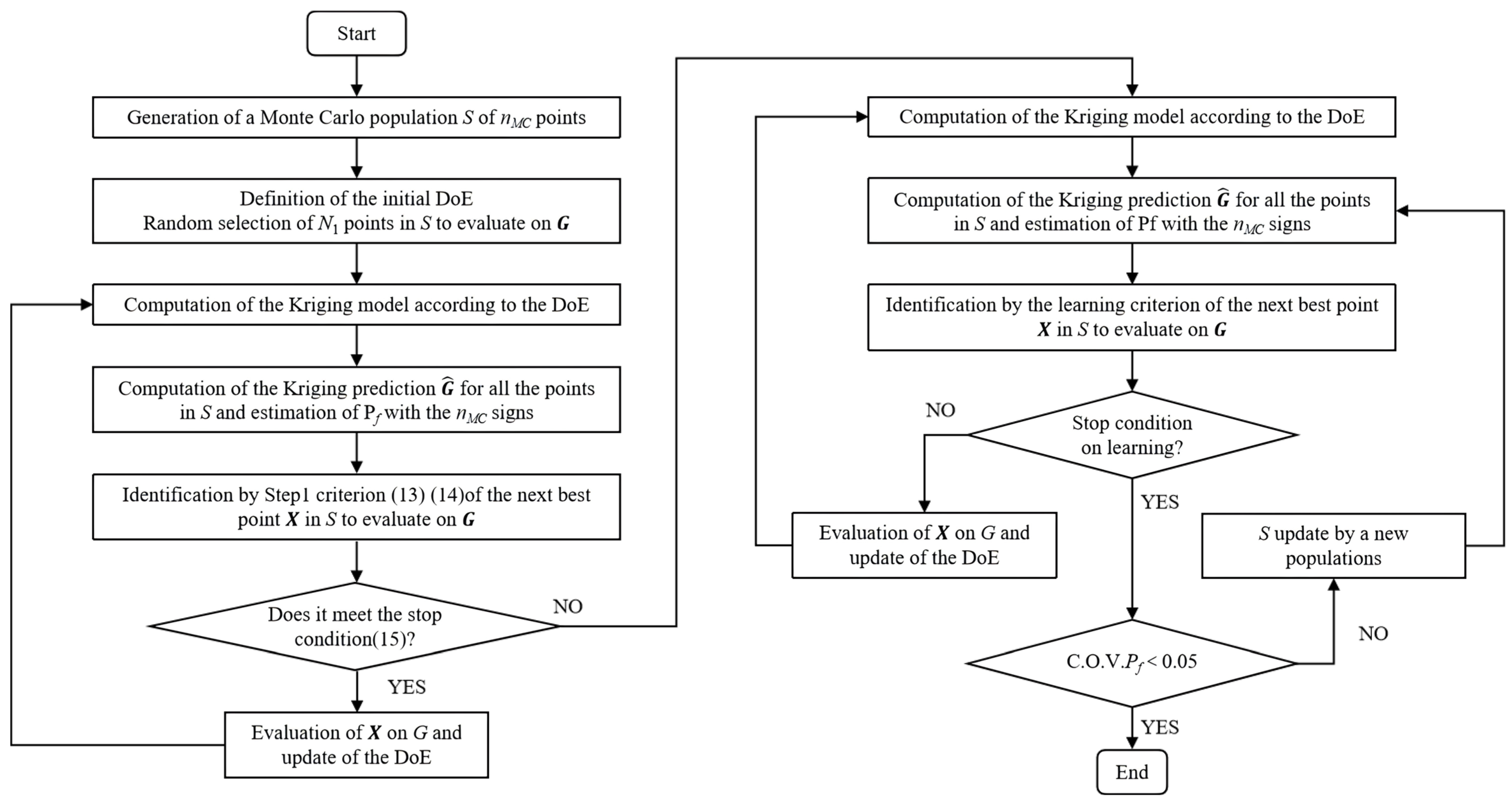
The procedures of the two-stage AK-MCS method are shown in Figure 1. The specific execution procedures can be described separately in two parts: Stage 1: Learning function L and Stage 2: Learning function U.

3.2.1. Stage 1: Learning Function L

In Stage 1: Learning function L, the Kriging model is regarded as a crude surrogate, so the selection strategy for the best next points is proposed to lie in the vicinity of the performance function. The strategy will first identify the design points that lie closest to the failure boundary, which are the points whose absolute values of the evaluation results are the closest to zero. Among these points, the one that is the farthest from the design of experiments will be selected as the best next point. In Learning function L, the specific execution stages are as follows.

A sample set of points for the Monte Carlo population was generated, and the selected best next points will be derived from it. Then, the initial experimental design employs the Latin Hypercube sampling technique to choose the minimum number of required sample points. Meanwhile, the responses of the sample points in the initial design of experiments will be obtained through experiments or simulations.

The crude Kriging model will be fit by the determined points and responses in the design of experiments. This crude Kriging model will be used to evaluate the prediction for all sample points. The MCS method will estimate the failure probability based on the signs of all sample points.

Learning function L will identify the best next point based on the evaluation of all sample points. The specific point selection strategy can be divided into the following steps:

The first step involves selecting the a points from the sample set that are closest to the limit state function, defined as those with the minimum absolute values of the predicted function responses. The parameter a is set as 0.01% of the total sample set size. This percentage was chosen based on a preliminary trade-off analysis: a smaller a may fail to capture sufficient candidates near the limit state surface, whereas a larger a may introduce points with larger absolute predicted responses, thereby reducing the localization efficiency of Stage 1. Generally, 0.01% of the Monte Carlo sample pool is not a very large number. For the standard Monte Carlo population size of $n_{\mathrm{M}\mathrm{C}\mathrm{S}}=6\times {10}^4$ used in this study, 0.01% corresponds to six candidate points, which was found to strike a reasonable balance between localization and diversity.

The selection strategy of Learning function L in the first step is building a collection, which can be expressed as follows:

$$\begin{array}{c}{L}_1\left(\mathit{X}\right)=\left\{y_1\left({\mathit{x}}_1\right),y_2\left({\mathit{x}}_2\right),\dots ,y_a\left({\mathit{x}}_a\right)\right\}\end{array}$$

(13)

where $L_1\left(\mathit{X}\right)$ is the set of a points from the sample set that are closest to the limit state function. In this set, $y_1\left({\mathit{x}}_1\right)=min\left|\widehat{\mathit{Y}}\left({\mathit{x}}_1\right)\right|$ and $y_a\left({\mathit{x}}_a\right) \mathrm{i}\mathrm{s} \mathrm{t}\mathrm{h}\mathrm{e} a-\mathrm{t}\mathrm{h} \mathrm{s}\mathrm{m}\mathrm{a}\mathrm{l}\mathrm{e}\mathrm{s}\mathrm{t} \mathrm{v}\mathrm{a}\mathrm{l}\mathrm{u}\mathrm{e}$.

The second stage entails calculating the distances between each of the selected a points and the sample set b. The point exhibiting the maximum distance from set b is identified as the best next point for this strategy. Here, set b refers to the DoE utilized for fitting the surrogate model in the preceding iteration.

The selection strategy of Learning function L in the second step is selecting the best next point, which can be expressed as follows:

$$\begin{array}{c}{L}_2\left({\mathit{x}}_{b+1}^{\ast }\right)\begin{array}{c}=max‖\mathit{X}-{\mathit{S}}_b‖\end{array}\end{array}$$

(14)

where ${\mathit{x}}_{b+1}^{\ast }$ is the best next point selected by Learning function L. $\mathit{X}$ is the set of a points from the first step of Learning function L and ${\mathit{S}}_b=\left\{{\mathit{x}}_1^{\ast },{\mathit{x}}_2^{\ast },\dots ,{\mathit{x}}_b^{\ast }\right\}$ is the DoE utilized for fitting the surrogate model, which refers to the existing training sample set.

At the same time, the response of the best next point should be evaluated immediately. The best next point and the response will be added to the design of experiments and will be used for the next round of Kriging model fitting.

Finally, the Kriging model will be judged to meet the requirements based on the convergence of the failure probability. If the convergence criterion can be met, then the process proceeds to Stage 2: Learning function U; otherwise, it will return to the stage of fitting the Kriging model and continue to evaluate the values of all points and the failure probability. Then, the new best next point will be selected again, thus forming an iterative optimization cycle. The stop condition of Learning function L can be expressed as follows:

$$\begin{array}{c}{cov}_1=\left|{\displaystyle \frac{p_{f\_N}-p_{f\_O}}{p_{f\_O}}}\right|<1\times {10}^{-3}\\ {cov}_2=\left|\widehat{\mathit{Y}}\left({\mathit{x}}_{b+1}^{\ast }\right)-\mathit{Y}\left({\mathit{x}}_{b+1}^{\ast }\right)\right|<1\times {10}^{-3}\end{array}$$

(15)

where ${cov}_1$ is the first convergence condition in Stage 1, which evaluates the error between two failure probabilities. $p_{f\_N}$ is the probability of failure in the current iteration and $p_{f\_O}$ is the probability of failure in the last iteration. ${cov}_2$ is the second convergence condition in Stage 2, which evaluates the error between the true and predicted values of the response at the current best next point. $\widehat{\mathit{Y}}\left({\mathit{x}}_{b+1}^{\ast }\right)$ is the predicted value and $\mathit{Y}\left({\mathit{x}}_{b+1}^{\ast }\right)$ is the true value.

3.2.2. Stage 2: Learning Function U

In Stage 2: Learning function U, the Kriging model will be regarded as a precise model. The main stages of this part are consistent with the AK-MCS method, to ensure that the final surrogate achieves the necessary accuracy. The strategy for determining the best next point is to enable the final surrogate to have better accuracy in Learning function U. The specific execution stages are as follows.

Following the design of experiments from Stage 1, continue to fit the Kriging model. The evaluations of all points are computed using the precise Kriging model, and the failure probability is considered too. Then, a best next point is determined by the learning criterion of Learning function U. The details of the learning criterion were introduced in Section 2.3. The response of the best next point will be immediately obtained by experiment or finite element analysis. The best next point and its associated response are integrated into the design of experiments, which was inherited from Stage 1 and applied to the subsequent surrogate fitting.

The convergence threshold for Learning Function U is that the minimum value of the stop condition should be greater than the threshold. The detailed introduction to the stop condition and the threshold is provided in Section 2.3. If the convergence criterion is not met, a new precise surrogate is fitted by the design of experiments; otherwise, it is necessary to further determine the convergence of the failure probability. If the convergence condition of the failure probability meets the requirements, the precise Kriging model is considered to be capable of meeting the required accuracy standards for the design.

4. Applications

This section introduces five reliability analysis cases to validate the feasibility of the two-stage AK-MCS method. In all numerical examples, the Monte Carlo population size is set to $n_{\mathrm{M}\mathrm{C}\mathrm{S}}=6\times {10}^4$. This sample size is chosen to achieve a satisfactory trade-off between computational cost and statistical accuracy, consistent with the settings widely adopted in the AK-MCS literature [8,24].

4.1. Numerical Case 1: Simple Performance Function

In case 1, a simple performance function is employed for verification. The two design variables are statistically independent and follow a normal distribution. The mean value of the design variables is (5.8, 2.5), and the standard deviation is (1, 1). The simple performance function is given by Equation (16):

$$\begin{array}{c}\mathit{Y}\left(x_1,x_2\right)=1-(0.9063x_1+0.4226x_2-6{)}^2-(0.9063x_1+0.4226x_2-6{)}^3\\ +0.6(0.9063x_1+0.4226x_2-6{)}^4+0.9063x_2-0.4226x_1\end{array}$$

(16)

The Two-Stage AK-MCS method is compared with the AK-MCS method to examine the difference in efficiency between the two while maintaining the same Kriging model accuracy. The correlation model of Kriging is Gaussian, and the regression model is constant in this case, which is the most common combination of fitting Kriging models. The Monte Carlo population size of this case is $n_{\mathrm{M}\mathrm{C}\mathrm{S}}=6\times {10}^4$ and it will be applied to the original MCS method, the AK-MCS method and the two-stage AK-MCS method. In this case, the number of sample points selected for the Latin Hypercube method was six, as the dimension of the design variables was 2.

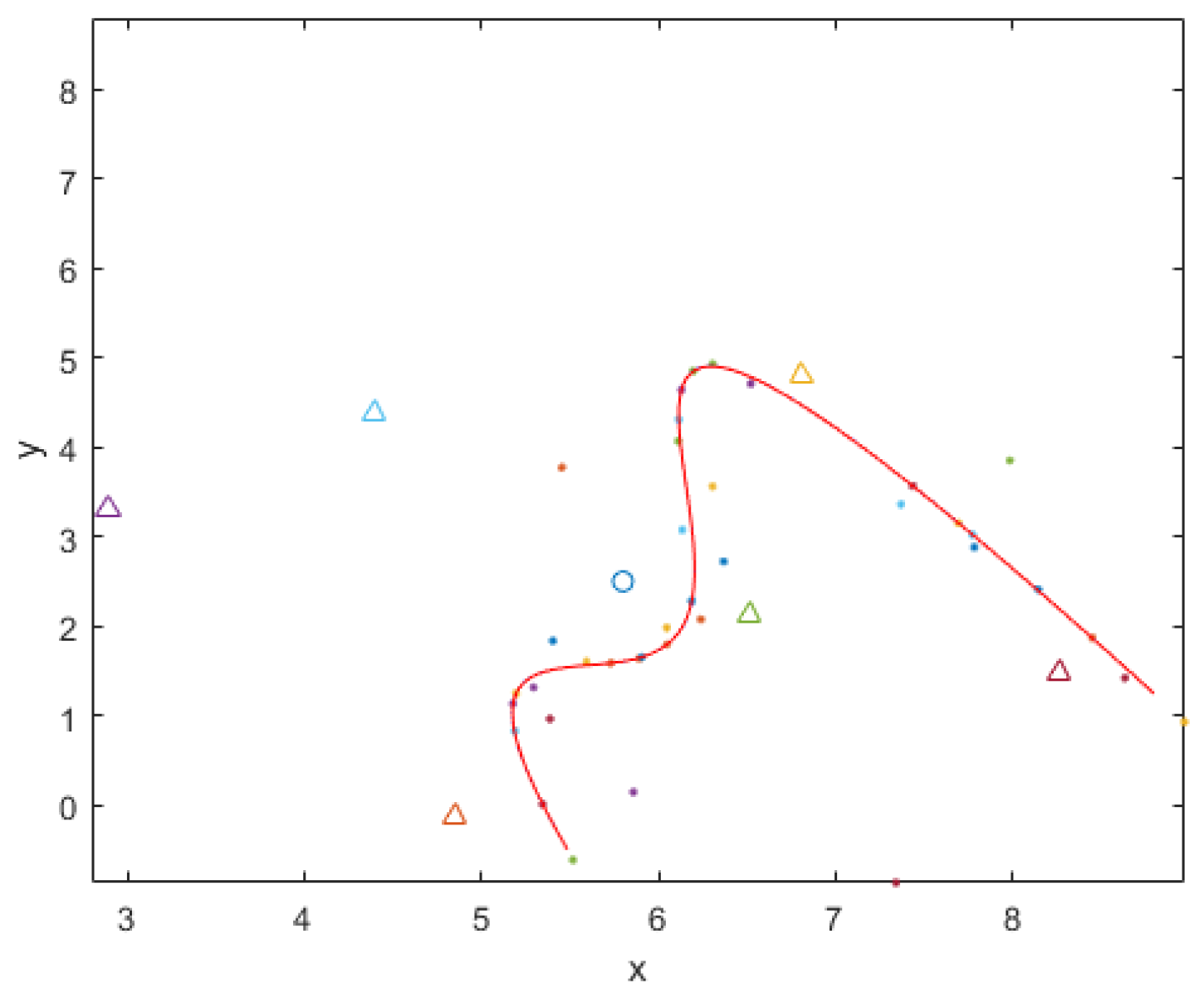
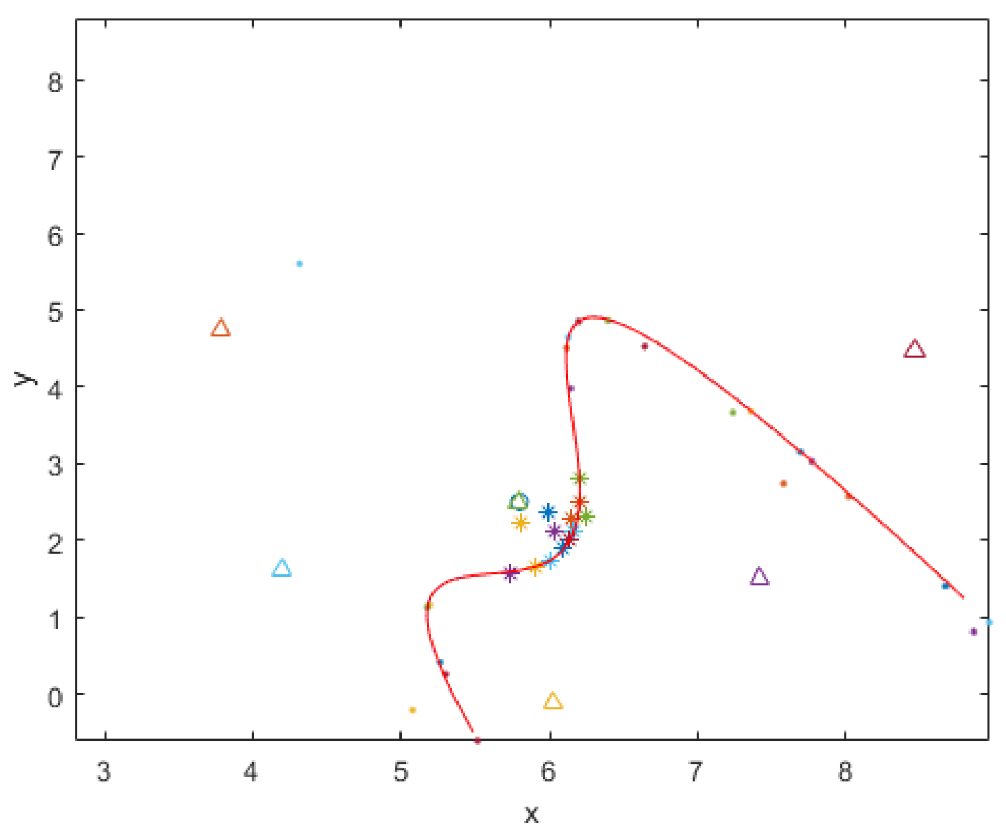
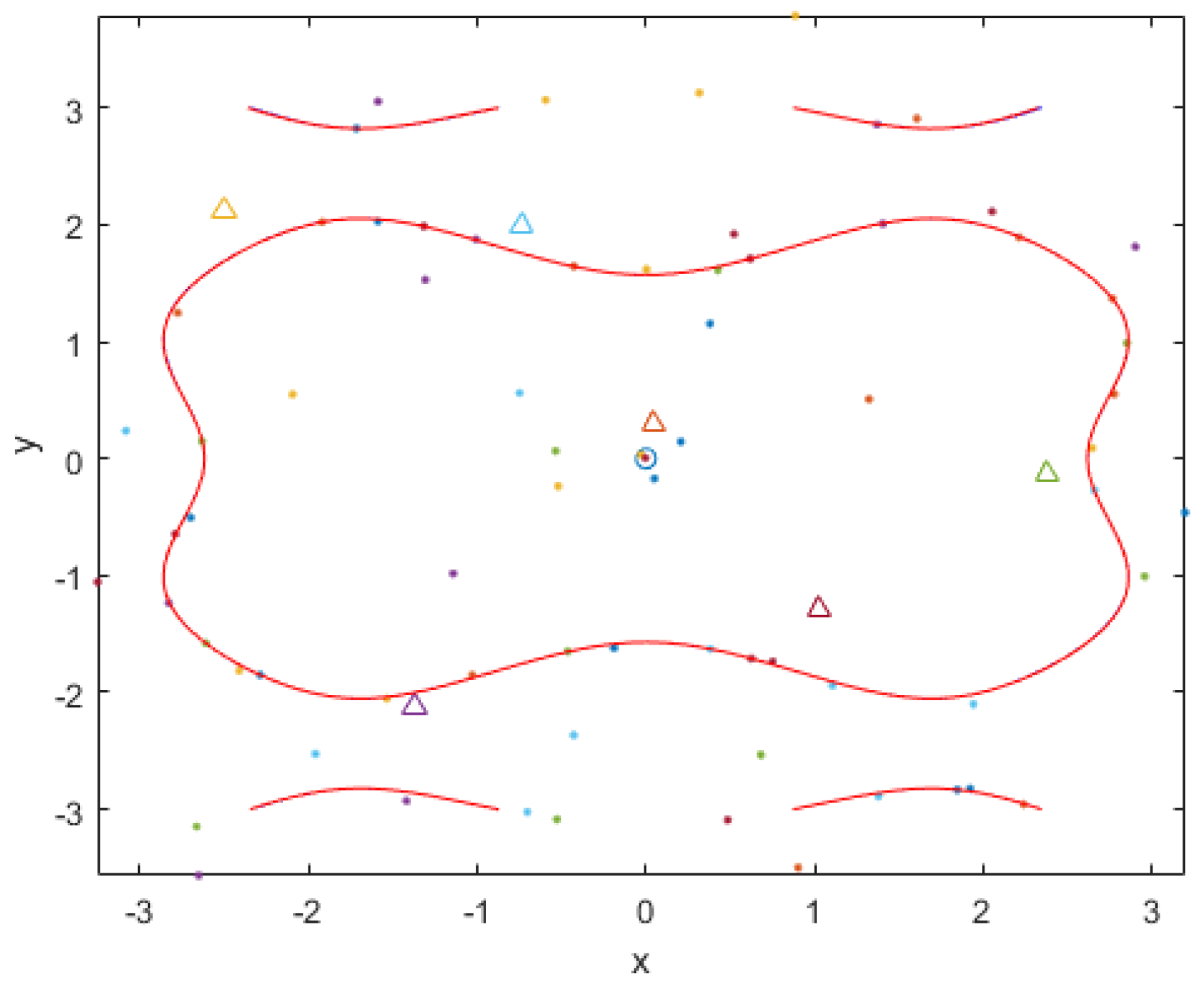
The process data and results of the AK-MCS method for handling numerical case 1 are shown in Figure 2. In this figure, ‘△’ represents the six sample points randomly determined by the Latin Hypercube method, and ‘.’ represents the best next sample points determined by the AK-MCS method. From the distribution of the determined points in the design domain, the AK-MCS method mainly selects sample points around the performance function, but they are rather scattered. Figure 3 shows the sample points selected and the results during the solution process of numerical case 1 by the two-stage AK-MCS method. In this figure, ‘*’ represents the points determined in Step 1 by Learning Function L of the Two-Stage AK-MCS method, and ‘.’ represents the sample points determined in Step 2 by Learning Function U. The sample points determined in Step 1 are almost located above the limit state function to establish a more precise Kriging model. In Step 2 of the Two-Stage AK-MCS method, the sample points are selected by Learning Function U, resulting in their primary clustering around the limit state function. As can be observed from the two figures, the Kriging models obtained by both methods demonstrate a high degree of consistency with the true performance function.

The results and process data of this case established by these three methods are shown in

Table 1. The results and process data of three methods for case 1.

Method	Ncall						Pf						Relative Error
	1	2	3	4	5	Ave.	1	2	3	4	5	Ave.
MCS	6 × 104						0.3935						-
AK-MCS	48	46	45	45	47	46.2	0.3935	0.3934	0.3935	0.3935	0.3935	0.3935	0
Two-stage AK-MCS	41	43	41	42	44	42.2	0.3935	0.3935	0.3935	0.3935	0.3935	0.3935	0

. Due to the randomness of sample selection in the Latin Hypercube method, the sample count selected in each case solution of AK-MCS and two-stage AK-MCS is not fixed. Therefore, the average value of multiple solutions is employed to ascertain the required sample count by the AK-MCS and two-stage AK-MCS methods to solve the problem. The number of sample points selected in three solution processes and the failure probability obtained from reliability analysis are presented in the table. The Two-Stage AK-MCS method selected an average of 42.2 sample points to solve the problem, which was fewer than the 46.2 sample points selected by the AK-MCS method. In other words, the Two-Stage AK-MCS method has an 8.6% higher solution efficiency compared to the AK-MCS method. In terms of accuracy, both methods achieved the same failure probability as the original MCS method.

4.2. Numerical Case 2: Highly Non-Linear Performance Function

There is a highly non-linear performance function, and its two design variables are independent of each other and follow a standard normal distribution. This function is given by Equation (17):

$$\mathit{Y}\left(x_1,x_2\right)={-x}_1\ast sin\left(1.2{\ast x}_1\right)-0.9\ast x_2\ast sin(2\ast x_2)$$

(17)

The correlation model of Kriging is Gaussian, and the regression model is constant in this case, which is the most common combination of fitting Kriging models. The Monte Carlo population size of this case is $n_{\mathrm{M}\mathrm{C}\mathrm{S}}=6\times {10}^4$ and will be applied to the original MCS method, the AK-MCS method and the two-stage AK-MCS method.

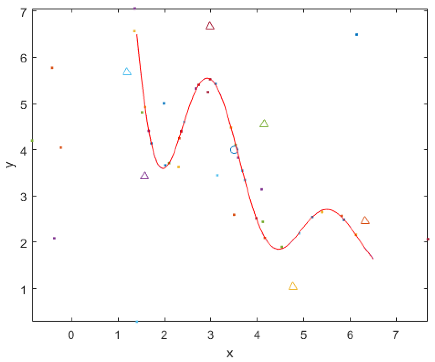
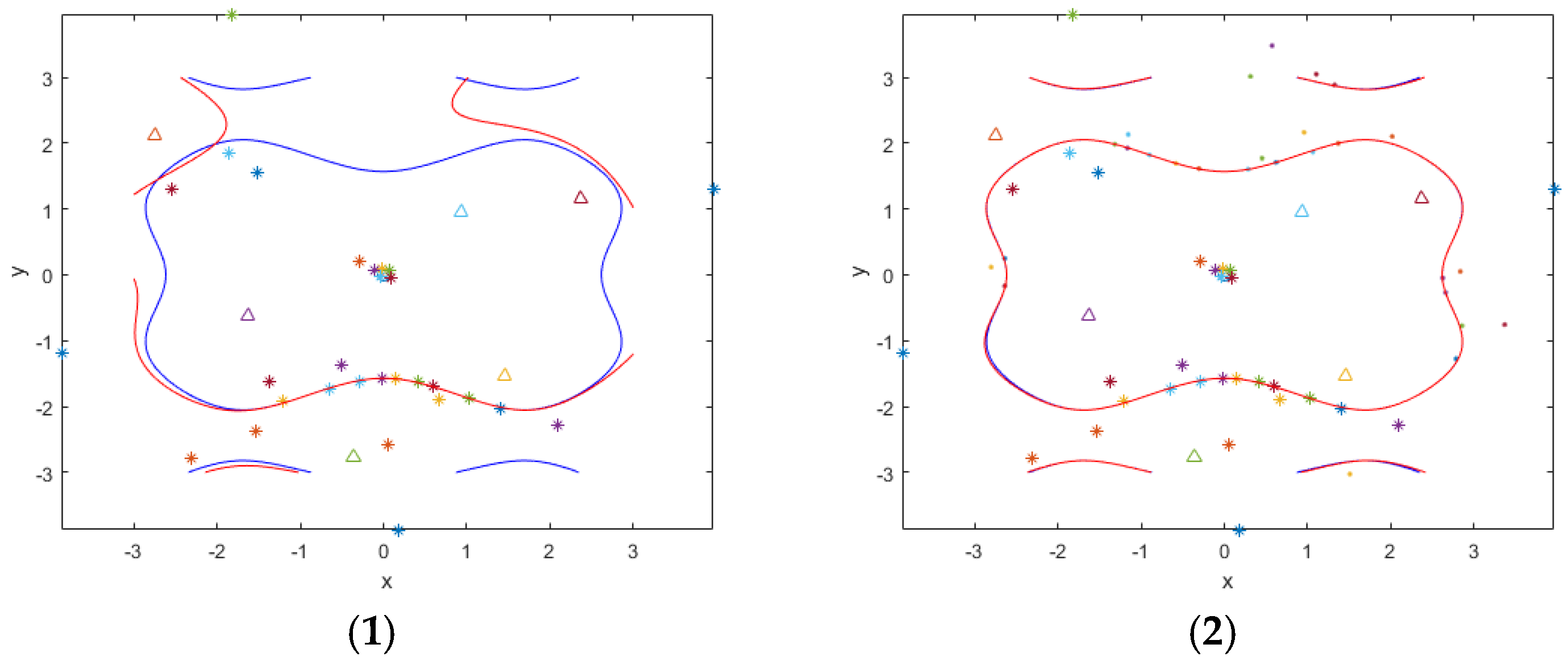
In Figure 4, the sample points determined by AK-MCS and the fitted Kriging model are presented. The sample points selected by the two-stage AK-MCS method are shown in Figure 5, where Figure 5(1) represents the samples determined through Learning Function L and the crude Kriging model, and Figure 5(2) shows all sample points selected in Step 1 and Step 2 of the final process, as well as the final precise surrogate obtained. In Figure 5(1), the true limit state function is the blue line, and the red line is the crude Kriging model.

The results and process data of this case established by these three methods are shown in

Table 2. The results and process data of three methods for case 2.

Method	Ncall						Pf						Relative Error
	1	2	3	4	5	Ave.	1	2	3	4	5	Ave.
MCS	6 × 104						0.9145						-
AK-MCS	77	78	75	74	77	76.2	0.9145	0.9145	0.9145	0.9145	0.9145	0.9145	0
Two-Stage AK-MCS	73	74	76	68	64	71	0.9145	0.9145	0.9145	0.9145	0.9145	0.9145	0

. The average sample count selected by the AK-MCS method and the Two-Stage AK-MCS method is 76.2 and 71, respectively. This indicates that the Two-Stage AK-MCS method reduces the selection of approximately 5.2 sample points when dealing with this case, thereby increasing the efficiency by 6.8% compared to the AK-MCS method. Furthermore, both methods performed equally well in terms of accuracy, achieving the same failure probability as the original MCS method.

4.3. Numerical Case 3: Highly Non-Linear Performance Function

Here is another highly non-linear performance function, and the design variables are normally distributed and statistically independent. The mean value of the design variables is (3.5, 4), and the standard deviation is (1, 1). This function can be expressed as Equation (18):

$$\mathit{Y}\left(x_1,x_2\right)={\displaystyle \frac{{(x}_1^2+4)\ast (x_2-1)}{20}}-sin\left(2.5{\ast x}_1\right)-2$$

(18)

The basic settings for solving numerical case 3 are the same as those for solving numerical case 2. For detailed settings, please refer to Section 4.2, Numerical Case 2: Highly non-linear performance function. No further elaboration is necessary.

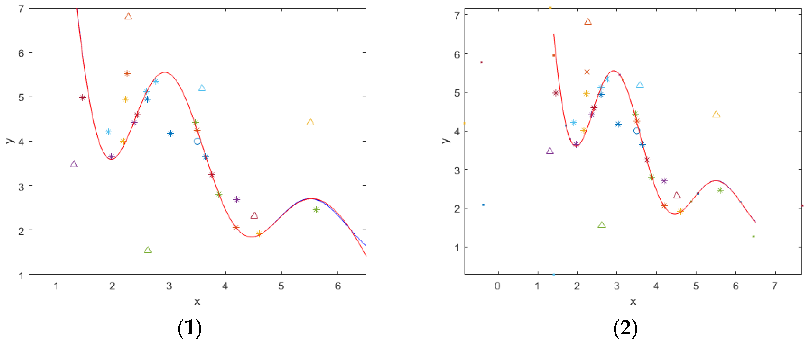
Figure 6 illustrates the samples selected via the AK-MCS method alongside the corresponding fitted Kriging surrogate model. Subsequently, the sampling procedure and model refinement of the Two-Stage AK-MCS method are detailed in Figure 7. This figure is partitioned into two subplots: Figure 7(1) corresponds to the samples determined by the Learning Function L in conjunction with an initial Kriging surrogate model, while Figure 7(2) presents the comprehensive set of samples acquired across both steps of the algorithm, together with the final refined Kriging surrogate model.

As comprehensively summarized in

Table 3. The results and process data of three methods for case 3.

Method	Ncall						Pf						Relative Error
	1	2	3	4	5	Ave.	1	2	3	4	5	Ave.
MCS	6 × 104						0.4540						-
AK-MCS	49	48	47	50	49	48.6	0.4540	0.4540	0.4540	0.4540	0.4540	0.4540	0
Two-Stage AK-MCS	45	44	44	46	46	45	0.4540	0.4540	0.4540	0.4540	0.4540	0.4540	0

, the experimental outcomes and procedural metrics generated by the three aforementioned methods for this case study are systematically presented. A comparative analysis of the mean sample sizes required by the AK-MCS method and the proposed Two-Stage AK-MCS method reveals values of 48.6 and 45, respectively. Notably, this disparity indicates that the Two-Stage AK-MCS method yields a reduction of approximately 3.6 samples relative to its counterpart when addressing the present problem, which corresponds to a 7.4% enhancement in terms of computational efficiency, surpassing the conventional AK-MCS approach. Importantly, despite the reduced sample size, both methods demonstrated comparable accuracy. Specifically, their estimated failure probabilities were statistically consistent with those derived from the original MCS method, underscoring the reliability of the two-stage framework without compromising predictive fidelity.

4.4. Numerical Case 4: Modified Rastrigin Function

This case is a modified Rastrigin function, which involves a non-convex and non-concave domain of the design space. Both design variables are mutually independent and obey a standard normal distribution. This function is given by Equation (19):

$$\mathit{Y}\left(x_1,x_2\right)=10-{\displaystyle \sum _{i=1}^2}{(x}_i^2-5\ast \mathrm{c}\mathrm{o}\mathrm{s}(2\ast \pi x_i))$$

(19)

The Monte Carlo population size of this case is $n_{\mathrm{M}\mathrm{C}\mathrm{S}}=6\times {10}^4$ and the correlation model of Kriging is Gaussian, and the regression model is constant in this case.

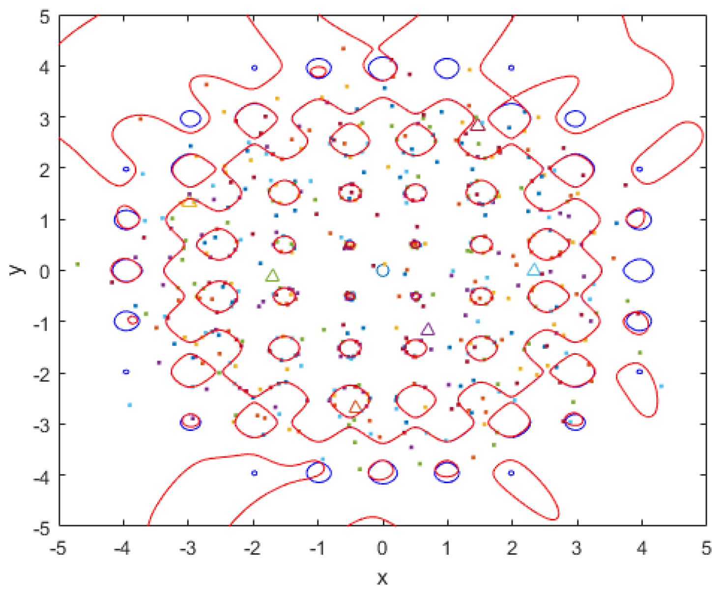
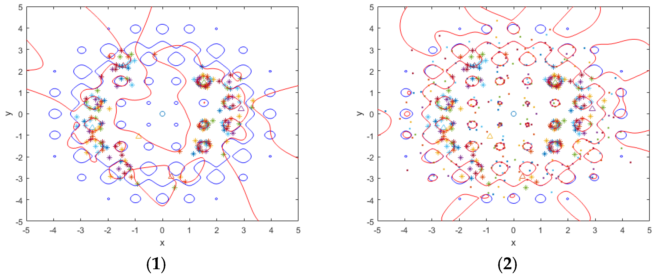
Figure 8 and Figure 9, respectively, show the sample points selected by the AK-MCS method and the Two-Stage AK-MCS method. In Figure 8, the sample points are evenly distributed throughout the design space. In Figure 9(1), the samples determined by Learning Function L are mostly located on the periphery of the design space and on the limit state function. In Figure 9(2), the comprehensive set of sample points acquired across both steps of the algorithm, together with the final refined Kriging surrogate model, are presented.

Table 4. The results and process data of three methods for case 4.

Method	Ncall						Pf						Relative Error
	1	2	3	4	5	Ave.	1	2	3	4	5	Ave.
MCS	6 × 104						0.0751						-
AK-MCS	530	534	523	573	584	548.8	0.0751	0.0751	0.0751	0.0751	0.0751	0.0751	0
Two-Stage AK-MCS	491	516	517	519	520	512.6	0.0751	0.0751	0.0751	0.0751	0.0751	0.0751	0

summarizes the experimental outcomes and procedural metrics produced by the three methods in this case study. A comparison of mean sample sizes shows that the AK-MCS method and Two-Stage AK-MCS method require 548.8 and 512.6 sample points on average, respectively. Notably, the Two-Stage AK-MCS method reduces the sample count by roughly 36.2 compared to its counterpart for this case, an improvement representing a 6.6% boost in computational efficiency over the conventional AK-MCS approach. Despite using fewer samples, both methods showed similar accuracy. Specifically, their estimated failure probabilities were statistically indistinguishable from those obtained via the original MCS method, highlighting the reliability of the proposed two-stage framework without sacrificing predictive fidelity.

4.5. Numerical Case 5: High-Dimensional Performance Function

The previous case discussed the effectiveness of the method in two-dimensional problems. This case will explore the effectiveness of the proposed method in a 40-dimensional performance function. This function is given by Equation (20):

$$\mathit{Y}\left(\mathit{x}\right)=d+3r\sqrt{d}-{\displaystyle \sum _{i=1}^d}{x}_i$$

(20)

where $d$ is the dimension of the design variables in the case. All random variables have a mean value of 1 and a standard deviation of 0.2. $r$ is 0.2 in this case. The Monte Carlo population size of this case is $n_{\mathrm{M}\mathrm{C}\mathrm{S}}=3\times {10}^5$ and the correlation model of Kriging is Gaussian, and the regression model is constant in this case.

The proposed Two-Stage AK-MCS method and AK-MCS method were employed to solve the high-dimensional complex problem, and the data shown in

Table 5. The results and process data of three methods for case 5.

Method	Ncall						Pf						Relative Error
	1	2	3	4	5	Ave.	1	2	3	4	5	Ave.
MCS	3 × 105						0.0751						-
AK-MCS	73	75	74	72	72	73.2	0.0013	0.0013	0.0013	0.0013	0.0013	0.0013	0
Two-Stage AK-MCS	70	72	72	74	71	71.8	0.0013	0.0013	0.0013	0.0013	0.0013	0.0013	0

were obtained. A comparison of mean sample sizes shows that the AK-MCS method and Two-Stage AK-MCS method require 73.2 and 71.8 sample points on average, respectively. Notably, the Two-Stage AK-MCS method reduces the sample count by roughly 1.8 compared to its counterpart for this case, an improvement representing a 2.0% boost in computational efficiency over the conventional AK-MCS approach.

4.6. Engineering Case: High-Speed Electric Spindle Considering Bearing Preload Force

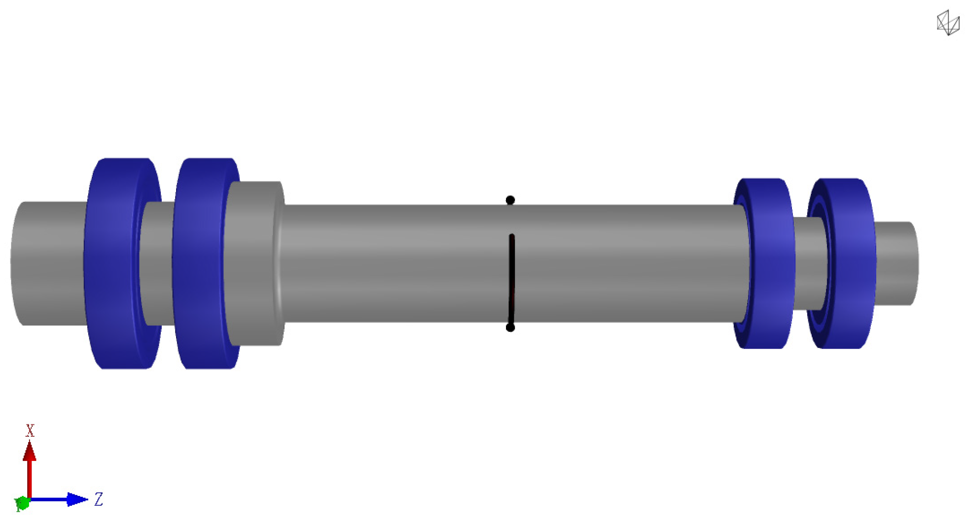
The high-speed electric spindle, as the core component of the power system in CNC machine tools, has attracted extensive attention due to reliability issues arising from the coupling effect of multiple physical fields such as electromechanical and hydromechanical. The high-speed electric spindle system can be simplified as shown in Figure 10, which includes the spindle and four bearings. In this case, the total length of the electric spindle is 285 mm. The front supporting bearing uses two identical angular contact ball bearings of model 7008, while the rear supporting bearing uses two identical angular contact ball bearings of model 7006. Both the front and rear supporting bearings are pre-tightened with fixed pressure. The maximum operating speed of the electric spindle is 18,000 r/min.

It was found that the preload of the bearings affects the stiffness and strength of the spindle. When installing the electric spindle, the preload may vary randomly during the setting process due to human factors during the installation. This can cause changes in the strength of the spindle and may lead to changes in the reliability of the electric spindle system. Therefore, it is of great significance to evaluate the reliability of the electric spindle system under the influence of the randomness of the preload.

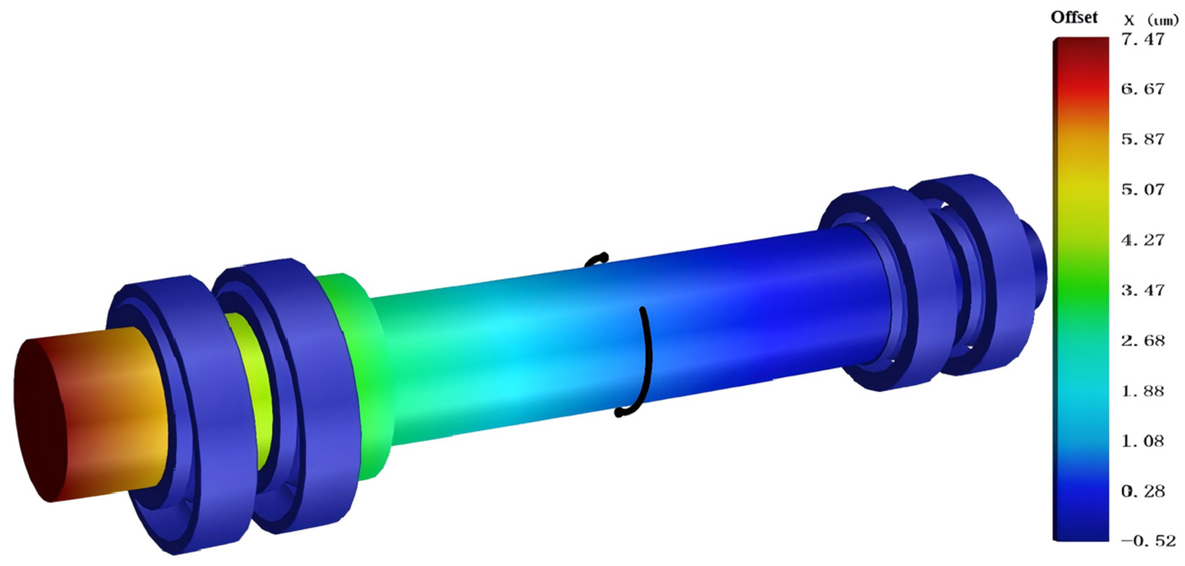
In this engineering case, the design variables $\left(x_1,x_2\right)$ are the preloads of the front supporting bearings and the rear supporting bearings, respectively, which follow a normal distribution. The front supporting bearing preloads are set to 200 N, and the rear supporting bearing preloads are set to 130 N. The constraint was the axial offset at the end of the high-speed electric spindle, which was obtained through the Romax software analysis, as shown in Figure 11. This function is given by Equation (21):

$$\mathit{Y}\left(x_1,x_2\right)={Model}_{Kriging}\left(x_1,x_2\right)-7$$

(21)

The Monte Carlo population size of this case is_MCS = 6 × 10⁴ and the correlation model of Kriging is Gaussian, and the regression model is constant in this case.

The AK-MCS method and the Two-Stage AK-MCS method are used to calculate the failure probability of the high-speed electric spindle under the influence of the randomness of the preloads. The data for the two methods are shown in

Table 6. The results and process data of two methods for the engineering case.

Method	Ncall				Pf
	1	2	3	Ave.	1	2	3	Ave.
MCS	-				-
AK-MCS	762	809	849	807	0.6363	0.6358	0.6360	0.6360
Two-Stage AK-MCS	716	679	782	726	0.6366	0.6366	0.6361	0.6364

. The AK-MCS method selected an average of 807 sample points to construct the Kriging model, whereas the Two-Stage AK-MCS method required an average of only 726 sample points for model construction. Regardless, the failure probabilities estimated by the AK-MCS and Two-Stage AK-MCS methods exhibit negligible differences, with values of 0.6360 and 0.6364, respectively. Therefore, based on the data presented in the table, the Two-Stage AK-MCS method demonstrates a 9.5% improvement in efficiency compared to the AK-MCS method for evaluating this engineering problem, while simultaneously ensuring the accuracy of the estimated failure probability.

5. Conclusions and Discussion

In this paper, a Two-Stage AK-MCS approach is introduced to improve the efficiency of both Kriging model establishment and failure probability assessment. The method divides the strategy for selecting the best next points in the AK-MCS method into two sequential phases within a single surrogate framework: Stage 1 involves selecting sample points lying on the limit state surface using Learning Function L, and Stage 2 determines the best next points using Learning Function U of the AK-MCS method. The surrogate in Stage 1 is regarded as a crude one. Once the failure probability assessment of the crude surrogate reaches convergence accuracy, it is considered a precise Kriging model, and the process proceeds to Stage 2.

The primary advantage of this task-decomposition strategy is its adaptive allocation of computational effort. By separating boundary localization from probability refinement, the method avoids the inefficiency of applying a uniform local-refinement criterion across the entire design space during the early iterations. Comparative studies across six benchmark cases—including highly nonlinear two-dimensional functions, a six-dimensional problem, and a high-speed electric spindle engineering application—demonstrate that the Two-Stage AK-MCS method reduces the average number of function evaluations by 3.0% to 10.0% compared to the standard AK-MCS method, while maintaining zero relative error in failure probability estimation. For the engineering case where each evaluation requires an expensive Romax finite element analysis, the proposed method saves an average of 81 function evaluations, which translates directly into substantial wall-clock time savings given that the Kriging fitting overhead is negligible.

The Two-Stage AK-MCS framework is particularly suitable for reliability analysis scenarios where the limit-state function is expensive to evaluate, and the failure boundary exhibits moderate to high nonlinearity. However, there are still some important issues that the Two-Stage AK-MCS method fails to consider. For instance, when the failure probability is minimal, how to conduct the convergence calculation for failure probability in the Two-Stage AK-MCS method. In future work, a more comprehensive approach will be our goal.

References

1. Liu, X.; Yin, L.; Hu, L.; Zhang, Z. An efficient reliability analysis approach for structure based on probability and probability box models. Struct. Multidiscip. Optim. 2017, 56, 167–181. [Google Scholar] [CrossRef] [Scilit]
2. Meng, Z.; Zhang, D.; Li, G.; Yu, B. An importance learning method for non-probabilistic reliability analysis and optimization. Struct. Multidiscip. Optim. 2019, 59, 1255–1271. [Google Scholar] [CrossRef] [Scilit]
3. Xie, B.; Wang, Y.; Zhu, Y.; Lu, F. A novel reliability analysis method combining adaptive relevance vector machine and subset simulation for small failure probability. Struct. Multidiscip. Optim. 2023, 66, 47. [Google Scholar] [CrossRef] [Scilit]
4. Ghorbani, M.; Nourelfath, M.; Gendreau, M. Stochastic programming for selective maintenance optimization with uncertainty in the next mission conditions. Reliab Eng. Syst. Saf. 2024, 241, 109624. [Google Scholar] [CrossRef] [Scilit]
5. Xia, Z.; Wu, Y.; Sun, J.; Yan, H.; Tian, J.; Wang, H.; Li, S. Analysis of cage dynamic characteristics for high-speed full ceramic ball bearing under non-lubrication condition. Nonlinear Dyn. 2024, 112, 6947–6966. [Google Scholar] [CrossRef] [Scilit]
6. Yang, M.; Zhang, H.; Zhang, D.; Han, X.; Li, Q. Time-variant reliability-based robust optimization for structures with material degradation. Comput Methods Appl. Mech. Eng. 2024, 432, 117337. [Google Scholar] [CrossRef] [Scilit]
7. Yu, S.; Fan, W.; Li, Z. A new active learning Kriging method with pseudo Kriging strategy for structural reliability analysis. Struct. Multidiscip. Optim. 2025, 68, 123. [Google Scholar] [CrossRef] [Scilit]
8. Echard, B.; Gayton, N.; Lemaire, M. AK-MCS: An active learning reliability method combining Kriging and Monte Carlo Simulation. Struct. Saf. 2011, 33, 145–154. [Google Scholar] [CrossRef] [Scilit]
9. Tabandeh, A.; Jia, G.; Gardoni, P. Langevin importance sampling for reliability analysis. Reliab Eng. Syst. Saf. 2026, 266, 111634. [Google Scholar] [CrossRef] [Scilit]
10. Wu, P.; Li, Y. Adaptive kriging model-based structural reliability analysis under interval uncertainty with incomplete data. Struct. Multidiscip. Optim. 2023, 66, 22. [Google Scholar] [CrossRef] [Scilit]
11. Chiralaksanakul, A.; Mahadevan, S. First-Order Approximation Methods in Reliability-Based Design Optimization. J. Mech. Des. 2004, 127, 851–857. [Google Scholar] [CrossRef] [Scilit]
12. Zhang, J.; Du, X. A Second-Order Reliability Method With First-Order Efficiency. J. Mech. Des. 2010, 132, 101006. [Google Scholar] [CrossRef] [Scilit]
13. Chen, Z.; Wu, Z.; Li, X.; Chen, G.; Chen, G.; Gao, L.; Qiu, H. An accuracy analysis method for first-order reliability method. Proc. Inst. Mech. Eng. Part C J. Mech. Eng. Sci. 2019, 233, 4319–4327. [Google Scholar] [CrossRef] [Scilit]
14. Du, X. Unified Uncertainty Analysis by the First Order Reliability Method. J. Mech. Des. 2008, 130, 091401. [Google Scholar] [CrossRef] [Scilit]
15. Rackwitz, R.; Flessler, B. Structural reliability under combined random load sequences. Comput Struct. 1978, 9, 489–494. [Google Scholar] [CrossRef] [Scilit]
16. Yang, S.; Meng, D.; Yang, H.; Keshtegar, B.; De Jesus, A.M.P.; Zhu, S.-P. Adaptive Kriging-assisted enhanced sparrow search with augmented-Lagrangian first-order reliability method for highly efficient structural reliability analysis. Reliab Eng. Syst. Saf. 2026, 267, 111916. [Google Scholar] [CrossRef] [Scilit]
17. Du, X.; Guo, J.; Beeram, H. Sequential optimization and reliability assessment for multidisciplinary systems design. Struct. Multidiscip. Optim. 2008, 35, 117–130. [Google Scholar] [CrossRef] [Scilit]
18. Lin, H.; Zhang, X.-Y.; Zhao, Y.-G. A dimensional reduction outcrossing rate method for time-dependent system reliability analysis. Reliab Eng. Syst. Saf. 2026, 266, 111772. [Google Scholar] [CrossRef] [Scilit]
19. Maier, H.R.; Lence, B.J.; Tolson, B.A.; Foschi, R.O. First-order reliability method for estimating reliability, vulnerability, and resilience. Water Resour. Res. 2001, 37, 779–790. [Google Scholar] [CrossRef] [Scilit]
20. Wu, Z.; Chen, Z.; Chen, G.; Li, X.; Jiang, C.; Gan, X.; Gao, L.; Wang, S. A probability feasible region enhanced important boundary sampling method for reliability-based design optimization. Struct. Multidiscip. Optim. 2021, 63, 341–355. [Google Scholar] [CrossRef] [Scilit]
21. Bird, G.A. Monte-Carlo simulation in an engineering context. Prog. Astronaut Aeronaut. 1981, 74, 239–255. [Google Scholar] [CrossRef] [Scilit]
22. Sun, Z.; Wang, J.; Li, R.; Tong, C. LIF: A new Kriging based learning function and its application to structural reliability analysis. Reliab Eng. Syst. Saf. 2017, 157, 152–165. [Google Scholar] [CrossRef] [Scilit]
23. Ma, J.; Ren, Z.; Zhao, G.; Zhang, Y.; Koh, C.-S. A New Reliability Analysis Method Combining Adaptive Kriging With Weight Index Monte Carlo Simulation. IEEE Trans. Magn. 2018, 54, 7001904. [Google Scholar] [CrossRef] [Scilit]
24. Peijuan, Z.; Ming, W.C.; Zhouhong, Z.; Liqi, W. A new active learning method based on the learning function U of the AK-MCS reliability analysis method. Eng. Struct. 2017, 148, 185–194. [Google Scholar] [CrossRef] [Scilit]
25. Su, M.; Xue, G.; Wang, D.; Zhang, Y.; Zhu, Y. A novel active learning reliability method combining adaptive Kriging and spherical decomposition-MCS (AK-SDMCS) for small failure probabilities. Struct. Multidiscip. Optim. 2020, 62, 3165–3187. [Google Scholar] [CrossRef] [Scilit]
26. Betz, W.; Papaioannou, I.; Straub, D. Bayesian post-processing of Monte Carlo simulation in reliability analysis. Reliab Eng. Syst. Saf. 2022, 227, 108731. [Google Scholar] [CrossRef] [Scilit]
27. Feng, S.; Wang, L.; Dong, H.; Li, Y.; Wan, Z.; Guedes Soares, C. An active-learning method based on hierarchical Kriging model for multi-fidelity reliability analysis. Reliab Eng. Syst. Saf. 2026, 266, 111759. [Google Scholar] [CrossRef] [Scilit]
28. Bichon, B.J.; Eldred, M.S.; Swiler, L.P.; Mahadevan, S.; McFarland, J.M. Efficient Global Reliability Analysis for Nonlinear Implicit Performance Functions. AIAA J. 2008, 46, 2459–2468. [Google Scholar] [CrossRef] [Scilit]
29. Meng, Y.; Zhang, D.; Shi, B.; Wang, D.; Wang, F. An active learning Kriging model with approximating parallel strategy for structural reliability analysis. Reliab Eng. Syst. Saf. 2024, 247, 110098. [Google Scholar] [CrossRef] [Scilit]
30. Xiong, Y.; Sampath, S. A fast-convergence algorithm for reliability analysis based on the AK-MCS. Reliab Eng. Syst. Saf. 2021, 213, 107693. [Google Scholar] [CrossRef] [Scilit]
31. Sun, H.; Bao, Y. An active learning method based on Monte Carlo dropout neural network for high-dimensional reliability analysis. Reliab Eng. Syst. Saf. 2025, 262, 111169. [Google Scholar] [CrossRef] [Scilit]
Figure 1. The procedures of the two-stage AK-MCS method.
Mathematics 14 02995 g001
Figure 2. The sample points and the predictive function of the AK-MCS method in case 1.
Mathematics 14 02995 g002
Figure 3. The sample points and predictive function of the Two-Stage AK-MCS method in case 1.
Mathematics 14 02995 g003
Figure 4. The sample points and predictive function of the AK-MCS method in case 2.
Mathematics 14 02995 g004
Figure 5. The sample points and predictive function of the Two-Stage AK-MCS method in case 2.
Mathematics 14 02995 g005
Figure 6. The sample points and predictive function of the AK-MCS method in case 3.
Mathematics 14 02995 g006
Figure 7. The sample points and predictive function of the Two-Stage AK-MCS method in case 3.
Mathematics 14 02995 g007
Figure 8. The sample points and predictive function of the AK-MCS method in case 4.
Mathematics 14 02995 g008
Figure 9. The sample points and predictive function of the Two-Stage AK-MCS method in case 4.
Mathematics 14 02995 g009
Figure 10. Model of high-speed electric spindle system in Romax software (2024.1 HEXAGON).
Mathematics 14 02995 g010
Figure 11. The analysis results of the high-speed electric spindle system in Romax software.
Mathematics 14 02995 g011