Residual-Based Fractional-Order Model Predictive Control for Automated Co-Administration of Anesthetic Drugs

Abstract

Closed-loop regulation of the bispectral index (BIS) during propofol–remifentanil co-administration is challenging because of nonlinear drug interactions, patient variability, model uncertainty, external disturbances, and infusion constraints. This paper proposes a residual-based fractional-order model predictive control (RB-FOMPC) method within the Extended Prediction Self-Adaptive Control (EPSAC) framework. FOMPC is obtained by introducing fractional-order weights into the EPSAC cost function, while an inverse Hill mapping handles the nonlinear BIS–drug relationship outside the online quadratic programming problem. RB-FOMPC further augments the FOMPC prediction with a bounded prediction of future residual variation generated by a delayed low-order residual model. During a predefined induction window, the one-sided correction is applied according to a filtered BIS-derived effect-site residual indicating nominal-model underestimation. A normalized infusion-ratio parameter coordinates the propofol and remifentanil inputs. Monte Carlo analysis showed that RB-FOMPC preserved the nominal FOMPC performance under inter-patient variability and substantially reduced excessive BIS undershoot under intra-patient model perturbations. Overall, the simulation results indicate that the residual-based predictive correction can selectively reduce induction-phase BIS undershoot under the evaluated nominal-model-underestimation conditions, while preserving the nominal performance of FOMPC.

1. Introduction

Precise regulation of anesthetic drug delivery is essential for maintaining an appropriate depth of anesthesia, which is closely related to intraoperative safety and postoperative outcomes [1]. Closed-loop control of anesthetic infusion can reduce the risks of intraoperative awareness and adverse hemodynamic events, thereby improving the overall quality of anesthesia management [2]. Compared with single-drug administration, the co-administration of propofol and remifentanil poses a more challenging control problem because drug interaction nonlinearity, input coupling, patient variability, external disturbances, and safety constraints must be addressed simultaneously.

Closed-loop anesthesia systems must also account for measurement noise, device interference, and surgical stimulation, which may affect the patient’s depth of anesthesia. In addition, due to the variety of surgical types, control structures may range from SISO to MIMO formulations, which also poses a challenge in the construction of control systems [3,4,5]. In classic anesthesia control, the anesthesiologist manually manipulates each anesthesia subprocess, performing appropriate drug infusions according to the patient’s specific signs. However, the process faces many challenges: significant pharmacodynamic differences between individual patients, nonlinear dynamics of the drug (such as the combined role of propofol and remifentanil in the patient’s anesthesia process) [6], and strict constraints in clinical scenarios (such as dose safety range, real-time regulation requirements). The complexity of these relationships presents a significant challenge for anesthesiologists; hence, the introduction of automatic control systems during anesthesia is both necessary and justified [7]. The precise control of anesthetic drugs is based on the pharmacokinetic/pharmacodynamic (PK/PD) model, which is used to describe the absorption, distribution, metabolism, and clearance of drugs in the body. Nevertheless, accurately characterizing drug accumulation effects and inter-individual variability remains challenging in anesthesia modeling, as reflected in commonly used models such as the Marsh model for propofol and the Minto model for remifentanil [8,9,10].

Among the available control strategies, PID-based methods remain widely used because of their simple structure, fast response, and acceptable disturbance rejection in practical anesthesia applications [11,12,13]. Despite these advantages, PID controllers generally lack prediction capability and do not explicitly incorporate clinical constraints into the control design. As a result, their performance may become insufficient when the process is strongly nonlinear, subject to model uncertainty, or required to satisfy stringent safety limits on drug administration.

Model predictive control (MPC) is well suited to anesthetic drug infusion because of its receding-horizon optimization mechanism, feedback correction, and explicit ability to handle multivariable constraints [14,15,16]. By exploiting a patient model, MPC can dynamically adjust the infusion profile according to the patient’s real-time response. In practice, however, the performance of conventional MPC may deteriorate in the presence of patient-model mismatch, strong nonlinearities, and patient variability. To alleviate these difficulties, several extensions have been proposed. For example, external predictors have been incorporated into MPC frameworks to compensate for process nonlinearities and improve robustness [17]. Event-based predictive control strategies have also been investigated to reduce unnecessary control updates while maintaining acceptable regulation performance [18,19]. Recent multiagent control studies have also addressed consensus tracking under asynchronous cooperation–competition interactions, illustrating the increasing attention paid to complex coordination and information-exchange conditions [20]. In addition, Extended Prediction Self-Adaptive Control (EPSAC), as a predictive control strategy within the MPC family, has shown good performance in anesthesia-related applications [21]. Fractional-order model predictive control (FOMPC) has attracted increasing attention in engineering systems because it provides additional flexibility in shaping the trade-off between tracking performance and control effort [22,23,24,25]. Recent studies have also indicated the potential of fractional-order concepts in anesthesia control [26,27]. However, the control performance of model predictive control is highly dependent on model accuracy; therefore, several online model identification schemes have also been proposed [28,29]. Because online identification requires a certain amount of time and the induction-phase delay and insufficient early observations prevent timely identification-based protection, these methods are not well suited to effectively mitigate excessive BIS undershoot during the induction phase.

The main contributions of this study are summarized as follows. The controller is developed sequentially from an EPSAC baseline to FOMPC and then to RB-FOMPC, while the inverse two-drug Hill reference mapping, current filtered effect-site residual feedback, nominal prediction model, infusion constraints, and receding-horizon QP structure are shared by all three controllers. First, FOMPC is obtained by replacing the conventional cost function in EPSAC with fractional-order weights. Second, a residual-based prediction method is incorporated into the FOMPC framework to compensate for patient-model mismatch during the induction phase, thereby reducing excessive BIS undershoot and improving safety-related BIS metrics during induction. This bounded correction is activated only during induction under a predefined condition, while the original decision variables, constraints, and QP structure are retained. Finally, Monte Carlo simulations are conducted to evaluate controller performance under inter-patient variability and intra-patient model mismatch. The comparison between EPSAC and FOMPC is used to examine the effect of the fractional-order cost function during the maintenance phase, while the comparison between FOMPC and RB-FOMPC is used to examine the additional effect of residual-based prediction on induction-phase BIS undershoot.

2. System Modeling and Controller Design

2.1. PK/PD Model for Drug Co-Administration

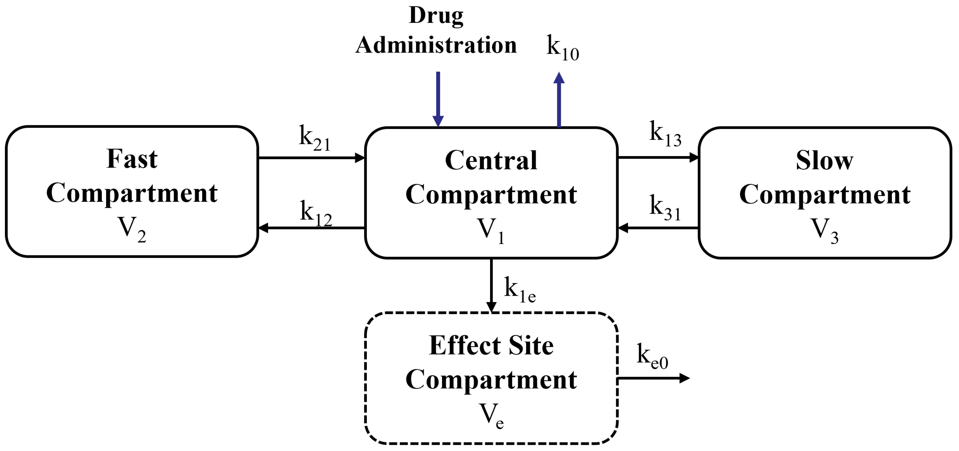
A three-compartment PK model with an additional effect-site compartment was used to describe the distribution, elimination, and delayed pharmacodynamic action of each drug. The three-compartment model is widely used to describe drug distribution and elimination in anesthesia modeling [30]. Generally, the three-compartment model is divided into a fast-response part (such as blood) and two slow-response parts (such as muscle and fat). The specific relationship between them is shown in Figure 1.

In the open-access simulation database from Ghent University, a hypothetical effect-site compartment is included to represent the delayed transport of the drug to its site of action [7]. The constant $k_{ij}$ represents the rate of drug transfer from the i-th compartment to the j-th compartment, and $k_{e0}$ represents the effect-site elimination rate constant. The equivalent fourth-order model of the above relationship can be expressed as follows:

$$\left[\begin{array}{c}{\dot{x}}_1\\ {\dot{x}}_2\\ {\dot{x}}_3\\ {\dot{x}}_e\end{array}\right]={\left[\begin{array}{cccc}-(k_{10}+k_{12}+k_{13})& k_{21}& k_{31}& 0\\ k_{12}& -k_{21}& 0& 0\\ k_{13}& 0& -k_{31}& 0\\ k_{1e}& 0& 0& -k_{e0}\end{array}\right]}_{\mathbf{A}}\left[\begin{array}{c}{x}_1\\ x_2\\ x_3\\ x_e\end{array}\right]+{\left[\begin{array}{c}1\\ 0\\ 0\\ 0\end{array}\right]}_{\mathbf{B}}u\left(t\right)$$

(1)

where $x_1$ (mg/mL) represents the central-compartment concentration; $x_2$ (mg/mL) and $x_3$ (mg/mL) are the fast and slow compartment concentrations; $x_e$ represents the effect-site concentration in the hypothetical compartment; $u\left(t\right)$ indicates the infusion rate of the drug injected. Here, $\mathbf{A}$ and $\mathbf{B}$ denote the system matrix and input matrix, respectively. The PK model parameters are determined from patient characteristics such as age, sex, weight, and height [31].

The patient model in (1) is formulated in continuous time. The predictive controller is implemented at the sampling instants $t_k=k{T}_s$. Assuming that the infusion input is held constant over each sampling interval, the zero-order-hold discrete model used for prediction is as follows:

$${\mathbf{x}}_{k+1}={\mathbf{A}}_d{\mathbf{x}}_k+{\mathbf{B}}_d{u}_k$$

(2)

where ${\mathbf{A}}_d=e^{\mathbf{A}{T}_s},{\mathbf{B}}_d={\int }_0^{T_s}{e}^{\mathbf{A}\tau }\mathbf{B}d\tau$. The continuous-time PK/PD models of propofol and remifentanil are discretized separately using zero-order hold with the controller sampling period $T_s$. The input-effect delays are represented by delay-augmented discrete state-space models, with the delay length expressed in sampling steps. The effect-site concentration used by the pharmacodynamic model is obtained as:

$$C_e\left(k\right)={\mathbf{C}}_e{\mathbf{x}}_k,{\mathbf{C}}_e=\left[\begin{array}{cccc}0& 0& 0& 1\end{array}\right]$$

(3)

The same discretization is applied separately to the propofol and remifentanil models to obtain $C{e}_p\left(k\right)$ and $C{e}_r\left(k\right)$.

The Hill function is commonly used to describe the nonlinear relationship between effect-site concentration and pharmacodynamic response. For a single drug, the concentration–effect relationship is expressed as

$$E=E_0-{\displaystyle \frac{E_{max}·x_e^{\gamma }}{C_{50}^{\gamma }+x_e^{\gamma }}}$$

(4)

where E(%) represents the predicted effect of the drug; $E_0$ is the initial BIS value before anesthetic administration; $x_e$ represents the effect-site concentration at time t; $C_{50}$ is the concentration required to obtain $50\%$ of the maximum effect $E_{max}$(%); $\gamma$ is the Hill coefficient [32].

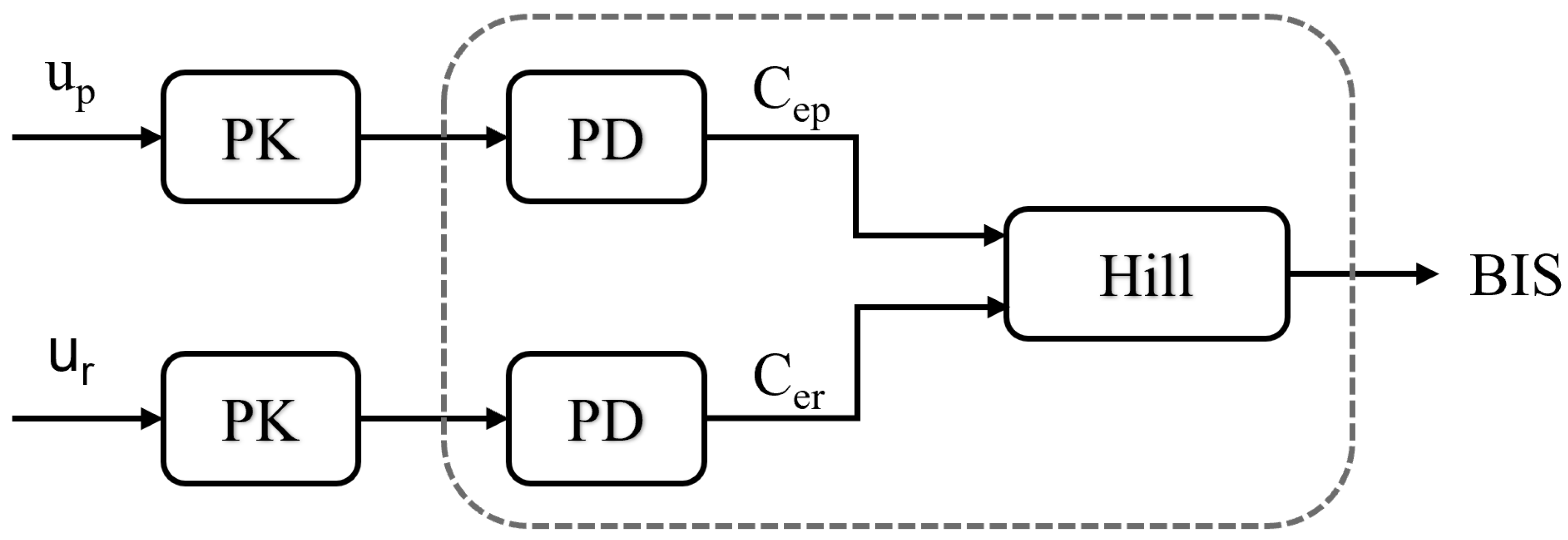
The overall PK/PD model is shown in Figure 2. The input drugs—propofol and remifentanil—are independently processed through their respective PK/PD models. The resulting parallel outputs are then combined via a nonlinear Hill function to determine the predicted BIS response. The pharmacodynamic behavior is thus realized through the integration of the PD blocks and the Hill function. The patient’s final depth of anesthesia is quantified by the BIS, which is described by the following equation:

$$BIS=E_0-E_{max}·{\displaystyle \frac{{(U_p+U_r+\sigma ·U_p·U_r)}^{\gamma }}{1+{(U_p+U_r+\sigma ·U_p·U_r)}^{\gamma }}}$$

(5)

where $U_p={\displaystyle \frac{C{e}_p}{C_{50,p}}}$ and $U_r={\displaystyle \frac{C{e}_r}{C_{50,r}}}$ are the standardized drug effect concentrations; $C_{50}$ is the half-effective concentration. $\sigma$ is the interaction parameter in the Hill response surface for propofol and remifentanil.

2.1.1. Patient Database

The patient dataset utilized in this study is sourced from an open-access model developed through a collaborative effort between Ghent University Hospital (Belgium) and the University Medical Center Groningen (The Netherlands). The details of the pharmacokinetic model are shown in

Table 1. The propofol-based patient database contains the corresponding variable values for the PK/PD model [7].

Index	Age (yrs)	Height (cm)	Weight (kg)	${\mathit{C}}_{50}$ (mg/mL)	$\mathit{\gamma }$ (-)
1	74	164	88	2.5	3
2	67	161	69	4.6	2
3	75	176	101	5	1.6
4	69	173	97	1.8	2.5
5	45	171	64	6.8	1.78
6	57	182	80	2.7	2.8
7	74	155	55	1.7	3.5
8	71	172	78	7.8	2.9
9	65	176	77	2.9	1.88
10	72	192	73	3.9	3.1
11	69	168	84	2.3	3.1
12	60	190	92	4.8	2.1
13	61	177	81	2.5	3
14	54	173	86	2.5	3
15	71	172	83	4.3	1.9
16	53	186	114	2.7	1.6
17	72	162	87	4.5	2.9
18	61	182	93	2.7	1.78
19	70	167	77	6.8	3.1
20	69	168	82	9.8	1.6
21	69	158	81	3.2	2.1
22	60	165	85	5.1	2.51
23	70	173	69	3.67	3.1
24	56	186	99	5.8	2.3
25	65	173	83	4.2	2.5

. In addition, based on the original patient dataset, this study adds a virtual Patient 25 with average values. The remifentanil PD parameters are based on commonly used values from Ref. [33], with $C_{50}=11.4$ (ng/mL) and $\gamma =2.5$.

2.1.2. Infusion-Ratio Coordination for Drug Co-Administration

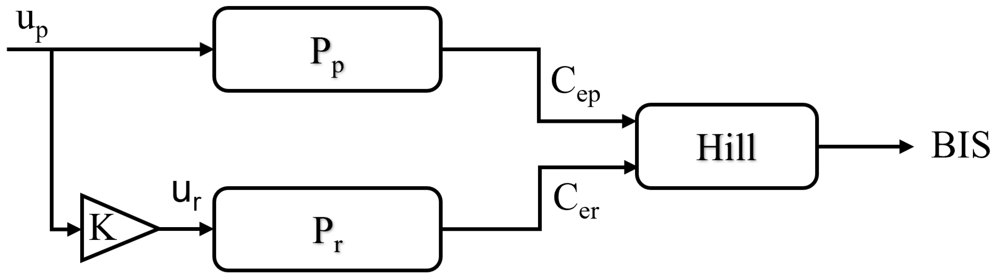
In propofol–remifentanil co-administration, the control problem is inherently two-input and one-output, which introduces redundancy because similar BIS responses may result from different drug combinations [34]. Without additional coordination, this may lead to undesirable input oscillations and an unreasonable balance between hypnosis and analgesia [35,36]. Therefore, introducing a normalized infusion ratio constraint is a practical way to regularize the control action, improve input smoothness, and provide a clinically interpretable parameter for coordinating the two drugs. To obtain smoother control inputs, a ratio parameter K is introduced to coordinate the infusion rates of the two drugs. This parameter can be adjusted by the anesthesiologist according to clinical requirements. Following Refs. [12,37], the ratio is set to the commonly used value of 2 in the subsequent simulations. This infusion ratio helps maintain clinically reasonable coordination between the two drugs. The modified PK/PD model is shown in Figure 3. The Hill block takes the propofol and remifentanil effect-site concentrations as its two inputs and internally normalizes them using the corresponding drug-specific $C_{50}$ values before calculating the combined BIS response.

2.2. Fractional-Order Model Predictive Control

2.2.1. Control System Constraints

The QP decision vector is the sequence of future increments in the propofol infusion input, with $u=u_p$: $\Delta \mathbf{U}={[\delta u\left(k\right|k),\delta u(k+1|k),\dots ,\delta u(k+N_u-1|k)]}^T$. The propofol infusion rate is bounded by $u_{\min }=0$ mg/kg∗min and $u_{\max }=1.25$ mg/kg∗min. The absolute infusion-rate constraints over the control horizon are

$$u_{\min }{\mathbf{1}}_{N_u}\le \mathbf{S}\Delta \mathbf{U}+u(k-1){\mathbf{1}}_{N_u}\le u_{\max }{\mathbf{1}}_{N_u}$$

(6)

where $\mathbf{S}\in {\mathbb{R}}^{N_u\times N_u}$ is a lower-triangular matrix of ones, and ${\mathbf{1}}_{N_u}$ is an $N_u$-dimensional vector of ones.

The input-increment bounds are $\delta u_{\min }=-0.04$ mg/kg∗min and $\delta u_{\max }=0.02$ mg/kg∗min, which are imposed directly on the QP decision vector:

$$\delta u_{\min }{\mathbf{1}}_{N_u}\le \Delta \mathbf{U}\le \delta u_{\max }{\mathbf{1}}_{N_u}.$$

(7)

The two drug inputs are coordinated through the normalized input-ratio parameter K, implemented as the fixed mapping $u_r=K{u}_p=Ku$ and $\delta u_r=K\delta u$. For $K=2$, the resulting remifentanil limits are $0\le u_r\le 2.5$ mcg/kg∗min and $-0.08\le \delta u_r\le 0.04$ mcg/kg∗min.

2.2.2. Mathematical Formulation

With the control problem formulated above, the constrained regulation problem is solved in a receding-horizon manner. The derivation proceeds from the EPSAC baseline to FOMPC and then to RB-FOMPC. At each sampling instant, the future input-increment sequence is optimized, while only the first increment is applied to the virtual patient [38,39]. The inverse Hill mapping and residual-estimation mechanism used to construct the predictor are described first.

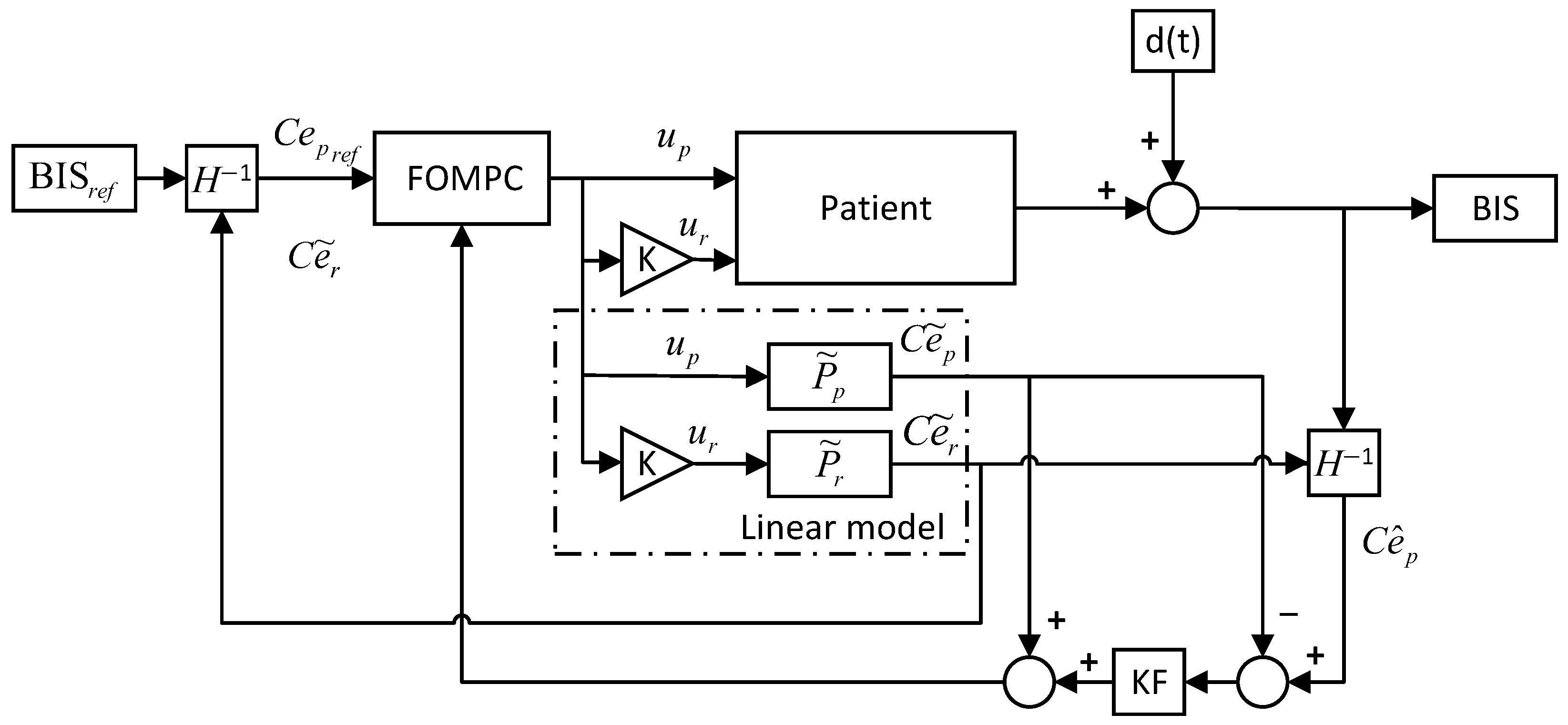
To address the strong nonlinearity caused by the Hill-type relationship between the combined drug effect and the BIS in the anesthesia process, an inverse Hill module $H^{-1}$ is incorporated into the control structure [17]. Its role is to transform the measured BIS, together with the estimated remifentanil effect-site concentration provided by the linear model, into an equivalent propofol-related effect quantity. In this way, the nonlinear part of the patient model is separated from the linear PK dynamics, allowing the controller to operate on a linear predictive model while still accounting for the nonlinearity of the process.

More specifically, the linear model provides the estimated remifentanil effect-site concentration $\tilde{C}{e}_r$, and the $H^{-1}$ module uses the measured BIS and $\tilde{C}{e}_r$ to reconstruct the corresponding combined drug-effect term

$$I={\left({\displaystyle \frac{E_0-BIS}{E_{max}-(E_0-BIS)}}\right)}^{{\displaystyle \frac{1}{\gamma }}}$$

(8)

where $I=U_p+U_r+\sigma U_p{U}_r$. Since $U_r$ is computed from $\tilde{C}{e}_r$, the corresponding estimate of the propofol effect-site concentration $\widehat{C}{e}_p$ can then be obtained through the inverse Hill mapping. Therefore, the $H^{-1}$ module serves as a nonlinear interface between the measured BIS and the linear predictive model, allowing the controller to update the output-related prediction without modifying the linear optimization structure of EPSAC.

If the nominal patient model were exact, the control problem could be handled using the linear predictive model. However, model accuracy cannot be guaranteed in practice. For this reason, an error compensation mechanism is further introduced.

To improve the smoothness of the compensation signal, a one-state Kalman filter is introduced in the error-compensation loop. At each controller sampling instant, the measured BIS and the nominal remifentanil effect-site concentration $\tilde{C}{e}_r\left(k\right)$ are supplied to the inverse Hill mapping to reconstruct the equivalent propofol effect-site concentration $\widehat{C}{e}_p\left(k\right)$. The scalar measurement supplied to the Kalman filter is therefore the reconstructed effect-site residual:

$$z_k=\widehat{C}{e}_p\left(k\right)-\tilde{C}{e}_p\left(k\right)$$

(9)

The residual is modeled using the discrete one-state random-walk system:

$${\xi }_k={\xi }_{k-1}+w_k,z_k={\xi }_k+v_k$$

(10)

where the state-transition and measurement coefficients are both equal to one. The process and measurement noises are assumed to be mutually independent zero-mean Gaussian variables:

$$w_k\sim \mathcal{N}(0,Q_{KF}),v_k\sim \mathcal{N}(0,R_{KF})$$

(11)

The filtered residual is denoted by $r\left(k\right)={\widehat{\xi }}_k$, and the effect-site concentration supplied to the controller is corrected as

$$C{e}_p\left(k\right)=\tilde{C}{e}_p\left(k\right)+r\left(k\right)$$

(12)

In the reported simulations, the sampled BIS was taken directly from the virtual-patient output, and no additional stochastic BIS measurement noise was injected. Thus, $Q_{KF}$ and $R_{KF}$ are estimator covariance settings. In this way, the dominant trend of the linear predictive model is preserved, while high-frequency fluctuations in the compensation signal are attenuated. The overall control structure is shown in Figure 4.

Within the FOMPC controller, the linear prediction model used by FOMPC is written as

$$y\left(k\right)=x\left(k\right)+n\left(k\right)$$

(13)

where $y\left(k\right)$ denotes the equivalent propofol effect-site concentration supplied to the EPSAC predictor, $x\left(k\right)$ is the output of the nominal discrete PK model, and $n\left(k\right)$ represents the estimated output mismatch. The current estimated output mismatch is held constant over the EPSAC prediction horizon.

$u\left(k\right)$ is the input of the model, representing the infusion rate of the drug. There is a dynamic relationship between $x\left(k\right)$ and $u\left(k\right)$, and $x\left(k\right)$ does not depend on the current $u\left(k\right)$, but on the previous $\left\{\begin{array}{c}u(k-1),u(k-2),\cdots \end{array}\right\}$ and $\left\{\begin{array}{c}x(k-1),x(k-2),\cdots \end{array}\right\}$. The relationship between them can be expressed by a general dynamic model:

$$x\left(k\right)=f\left[x\right(k-1),x(k-2),\cdots ,u(k-1),u(k-2),\cdots ]$$

(14)

In the EPSAC method, the control input sequence consists of two parts: one is the basic process input sequence at the future moment, and the other is the optimized input sequence at the future moment. The specific relationship is as follows:

$$u(k+j\mid k)=u_{base}(k+j\mid k)+\delta u(k+j\mid k)$$

(15)

The predicted output can be written as follows:

$$y(k+j\mid k)=y_{base}(k+j\mid k)+y_{opt}(k+j\mid k)$$

(16)

where $y_{base}(k+j\mid k)$ is obtained from $u_{base}(k+j\mid k)$. In the nonlinear case, the optimal control input is obtained through iterative optimization at the current sampling instant until the input increment becomes sufficiently small. In this study, the base future input sequence is held at the most recently applied input, such that $u_{\mathrm{base}}(k+j\mid k)=u(k-1)$, $j=0,\dots ,N_2-1$. Because a linear prediction model is used, iterative updating of the base input sequence is not required, and only the first element of the optimized control sequence is applied at each sampling instant. $y_{opt}(k+j\mid k)$ is obtained from $\delta u(k+j\mid k)$. $y_{opt}(k+j\mid k)$ is the cumulative effect of a series of pulse inputs and a step input.

Therefore, $y_{opt}(k+j\mid k)$ is expressed as follows:

$$\begin{array}{c}\hfill y_{opt}(k+j\mid k)=h_j\delta u(k\mid k)+h_{j-1}\delta u(k+1\mid k)+\cdots \\ \hfill +g_{j-N_u+1}\delta u(k+N_u-1\mid k)\end{array}$$

(17)

where $h_1,h_2,\cdots ,h_{N_2}$ are the coefficients of the system’s unit impulse response; $g_1,g_2,\cdots ,g_{N_2}$ are the coefficient of the system’s unit step response; $N_u$ is the control horizon; $N_2$ is the prediction horizon. The unit impulse response can be obtained simply by $h_j=g_j-g_{j-1}$.

By superimposing each step of the above formula, it can be written in the following matrix form:

$$\begin{array}{c}\hfill \left[\begin{array}{c}{y}_{opt}(k+N_1\mid k)\\ y_{opt}(k+N_1+1\mid k)\\ ⋮\\ y_{opt}(k+N_2\mid k)\end{array}\right]=\left[\begin{array}{ccccc}{h}_{N_1}& h_{N_1-1}& \dots & h_{N_1-N_u+2}& g_{N_1-N_u+1}\\ h_{N_1+1}& h_{N_1}& \dots & \dots & \dots \\ ⋮& ⋮& \ddots & ⋮& ⋮\\ h_{N_2}& h_{N_2-1}& \dots & h_{N_2-N_u+2}& g_{N_2-N_u+1}\end{array}\right]\left[\begin{array}{c}\delta u(k\mid k)\\ \delta u(k+1\mid k)\\ ⋮\\ \delta u(k+N_u-1\mid k)\end{array}\right]\end{array}$$

(18)

(18) can be written compactly as

$${\mathbf{Y}}_{opt}=\mathbf{G}·\Delta \mathbf{U}$$

(19)

The EPSAC prediction can then be derived from

$$\mathbf{Y}={\mathbf{Y}}_{base}+{\mathbf{Y}}_{opt}=\overline{\mathbf{Y}}+\mathbf{G}·\Delta \mathbf{U}$$

(20)

The standard EPSAC cost function is defined as

$${\displaystyle J_{MPC}={\displaystyle \sum _{j=N_1}^{N_2}}{\gamma }_j{[y_{ref}(k+j\mid k)-y(k+j\mid k)]}^2+{\displaystyle \sum _{j=0}^{N_u-1}}{\lambda }_j{\left[\delta u(k+j\mid k)\right]}^2}$$

(21)

where $y_{ref}(k+j\mid k)$ is the reference trajectory, ${\gamma }_j$ and ${\lambda }_j$ are weight coefficients, which are non-negative constants.

The matrix form of the cost function is expressed as

$$J_{MPC}={[({\mathbf{Y}}_{ref}-\overline{\mathbf{Y}})-\mathbf{G}\Delta \mathbf{U}]}^T\mathbf{Q}[({\mathbf{Y}}_{ref}-\overline{\mathbf{Y}})-\mathbf{G}\Delta \mathbf{U}]+\Delta {\mathbf{U}}^T\mathbf{P}\Delta \mathbf{U}$$

(22)

where ${\mathbf{Y}}_{ref}={[y_{ref}(k+N_1\mid k),\cdots ,y_{ref}(k+N_2\mid k)]}^T$ is the reference trajectory vector; $\overline{\mathbf{Y}}={[y_{base}(k+N_1\mid k),\cdots ,y_{base}(k+N_2\mid k)]}^T$ is the effect of base future control; $\Delta \mathbf{U}={[\delta u(k\mid k),\cdots ,\delta u(k+N_u-1\mid k)]}^T$ is the optimized future control action; $\mathbf{Q}=diag({\gamma }_{N_1},\cdots ,{\gamma }_{N_2})$ and $\mathbf{P}=diag({\lambda }_0,\cdots ,{\lambda }_{N_u-1})$ are weighting matrices.

By introducing fractional-order weighting, (21) is expressed as

$$\begin{array}{c}\hfill J_{FOMPC}={}^{\alpha }I_{N_1}^{N_2}{\gamma }_j{[y_{ref}(k+j\mid k)-y(k+j\mid k)]}^2\\ \hfill +{}^{\beta }I_0^{N_u-1}{\lambda }_j{\left[\delta u(k+j\mid k)\right]}^2\end{array}$$

(23)

The fractional-order cost function can be written in matrix form as follows:

$$\begin{array}{c}\hfill J_{FOMPC}={[({\mathbf{Y}}_{ref}-\overline{\mathbf{Y}})-\mathbf{G}\Delta \mathbf{U}]}^T\mathbf{Q}\mathrm{Y}(\alpha ,T_s)[({\mathbf{Y}}_{ref}-\overline{\mathbf{Y}})-\mathbf{G}\Delta \mathbf{U}]\\ \hfill +\Delta {\mathbf{U}}^T\mathbf{P}\Omega (\beta ,T_s)\Delta \mathbf{U}\end{array}$$

(24)

where $T_s$ is the sampling time. Based on the Grünwald–Letnikov definition of fractional calculus, the weighting matrices $\mathrm{Y}$ and $\Omega$ can be expressed in terms of the fractional-order operators ${}^{\alpha }I_{N_1}^{N_2}$ and ${}^{\beta }I_0^{N_u-1}$. The weighting matrices are determined by $\alpha$ and $\beta$.

$$\mathrm{Y}(\alpha ,T_s)=T_s^{\alpha }\mathrm{diag}(m_n,m_{n-1},\dots ,m_0),$$

(25)

where $m_j=v_j-v_{j-n}$, $n=N_2-N_1$, $v_k={(-1)}^k\left({\displaystyle \genfrac{}{}{0pt}{}{-\alpha }{k}}\right)$ for $k=N_1,\dots ,N_2$, and $v_k=0$ for $k<0$.

$$\Omega (\beta ,T_s)=T_s^{\beta }\mathrm{diag}(m_n,m_{n-1},\dots ,m_0),$$

(26)

where $m_j=v_j-v_{j-n}$, $n=N_u-1$, $v_k={(-1)}^k\left({\displaystyle \genfrac{}{}{0pt}{}{-\beta }{k}}\right)$ for $k=0,\dots ,N_u-1$, and $v_k=0$ for $k<0$.

2.2.3. Dynamic Residual-Based Predictive Compensation

Although the external predictor can compensate for the Hill-type nonlinear relationship, the prediction accuracy of FOMPC still depends on the consistency between the nominal PK/PD model and the actual patient dynamics. In particular, when the nominal model underestimates the actual pharmacodynamic sensitivity of the patient to propofol, the resulting patient-model mismatch may not yet be fully reflected in the current BIS measurement because of the pronounced delay inherent in the anesthetic drug-effect system. Consequently, the controller may generate an excessively large infusion input during the induction phase, leading to excessive BIS undershoot. To alleviate this issue, a dynamic residual-based predictive compensation is incorporated into the FOMPC prediction process.

The current equivalent propofol effect-site concentration residual is defined as $\Delta C{e}_p\left(k\right)=\widehat{C}{e}_p\left(k\right)-\tilde{C}{e}_p\left(k\right)$, where $\widehat{C}{e}_p\left(k\right)$ is reconstructed by the inverse Hill mapping and $\tilde{C}{e}_p\left(k\right)$ is obtained from the nominal linear PK model. The residual $\Delta C{e}_p\left(k\right)$ is filtered by the Kalman filter to obtain $r\left(k\right)$. In the proposed compensation logic, $r\left(k\right)>0$ is used to indicate a positive filtered effect-site residual. This condition corresponds to a case in which the nominal prediction underestimates the measured equivalent propofol-related drug effect, thereby increasing the risk of excessive BIS undershoot during induction. The residual increment and input increment are then defined as $\delta r\left(k\right)=r\left(k\right)-r(k-1)$ and $\delta u\left(k\right)=u\left(k\right)-u(k-1)$.

In this study, a low-order incremental residual model is employed to characterize the dynamic evolution of the filtered effect-site concentration residual:

$$\delta \widehat{r}(k+1|k)=c+\rho \delta r\left(k\right)+\eta r\left(k\right)+b\delta u(k-d)$$

(27)

where d denotes the discrete input-effect delay, and c, $\rho$, $\eta$, and b are the identified residual-model parameters.

For multi-step prediction, the residual increment is recursively computed as

$$\begin{array}{cc}\hfill \delta \widehat{r}(k+j|k)=& c+\rho \delta \widehat{r}(k+j-1|k)+\eta \widehat{r}(k+j-1|k)\hfill \\ & +b\delta u(k+j-1-d|k),\hfill \end{array}j=1,\dots ,N_2$$

(28)

The residual-based prediction is then updated by

$$\widehat{r}(k+j|k)=\widehat{r}(k+j-1|k)+\delta \widehat{r}(k+j|k),j=1,\dots ,N_2$$

(29)

The initial values are defined as

$$\widehat{r}\left(k\right|k)=r\left(k\right),\delta \widehat{r}\left(k\right|k)=r\left(k\right)-r(k-1)$$

(30)

For delayed input terms corresponding to past instants, the measured input history is used. Within the prediction horizon, the input increments are constructed from a preliminary FOMPC input obtained before solving the final QP and held constant over the horizon.

Therefore, the residual model generates the future residual-based prediction sequence

$$\widehat{\mathbf{R}}\left(k\right)=\left[\begin{array}{c}\widehat{r}(k+1|k)\\ \widehat{r}(k+2|k)\\ ⋮\\ \widehat{r}(k+N_2|k)\end{array}\right]$$

(31)

Since FOMPC already uses the current filtered residual $r\left(k\right)$ to correct the current effect-site state, RB-FOMPC does not repeatedly incorporate the full predicted residual. Instead, it compensates only for the variation in the future residual relative to the current residual:

$$\delta {\widehat{r}}_h(k+j|k)=\widehat{r}(k+j|k)-r\left(k\right),j=1,\dots ,N_2$$

(32)

Here, $\delta {\widehat{r}}_h(k+j|k)$ represents the predicted residual variation, rather than the full residual itself.

The RB-FOMPC prediction of the propofol effect-site concentration is then expressed as

$$C{e}_p^{\mathrm{RB}}(k+j|k)=\tilde{C}{e}_p(k+j|k)+r\left(k\right)+{\lambda }_g\left(k\right)g\left(k\right)\delta {\widehat{r}}_h(k+j|k),j=1,\dots ,N_2$$

(33)

Here, ${\lambda }_g\left(k\right)$ denotes the compensation gating coefficient, and $g\left(k\right)$ is the correction gain. Their activation logic, one-sided residual processing, and saturation settings are given in the parameter-selection section.

3. Results

3.1. Control System Tuning

During the tuning of the controller parameters, the sampling time $T_s$ and the length of the dead zone of the prediction $N_1$ are first determined. $T_s$ is set to 1 s due to limitations of the monitoring equipment. Since the model already incorporates a delay element, $N_1$ is set to 1. The controller parameters were selected by minimizing the IAE defined as

$${\displaystyle IAE={\displaystyle \sum _{k=0}^N}\left|e\left(k\right)\right|}$$

(34)

N is the total number of sampling points; $e\left(k\right)$ is the value of the error between the output value and the target value at the kth step.

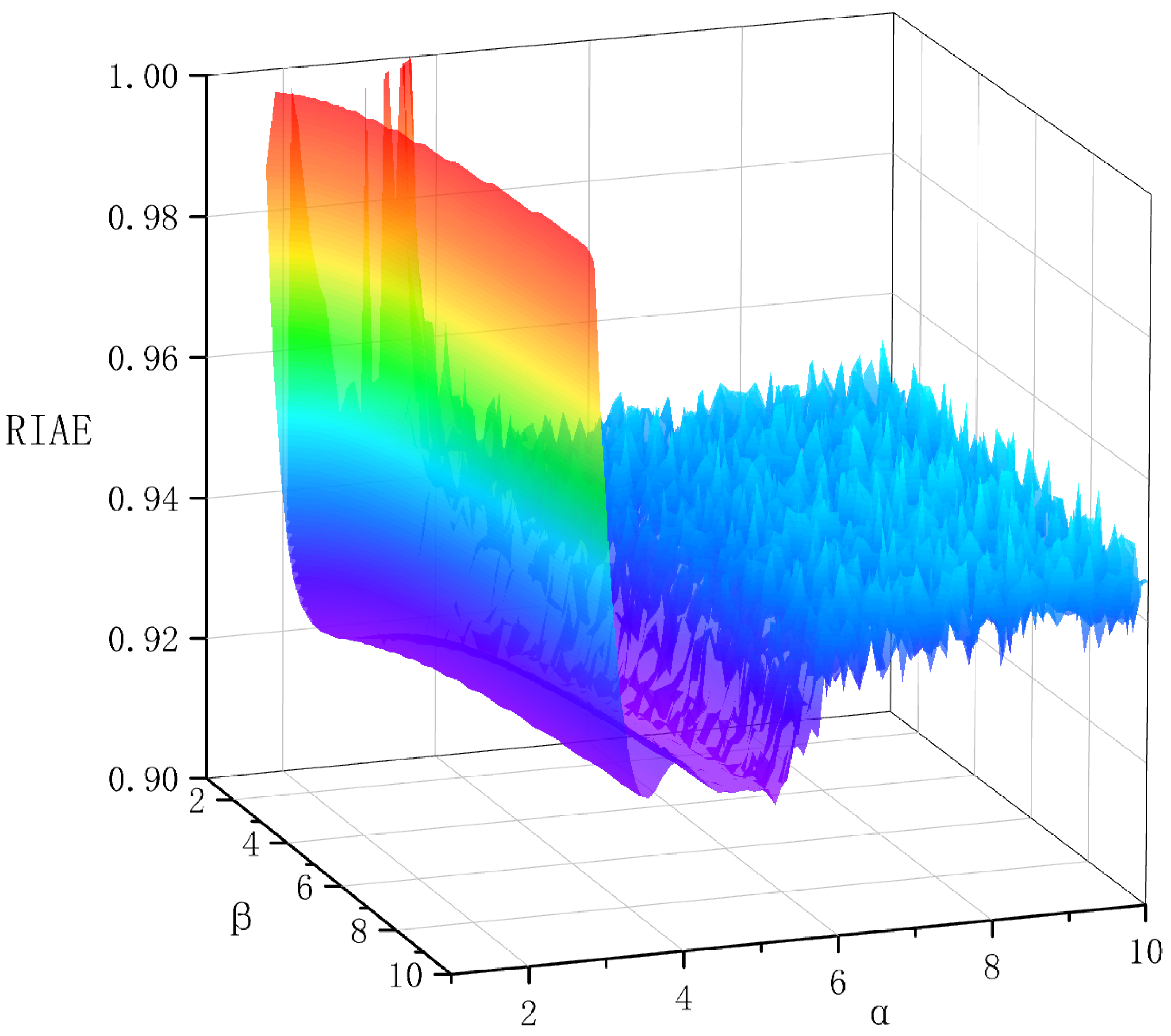
After determining the prediction horizon $N_2$ and the control horizon $N_u$, the corresponding $\alpha$ and $\beta$ parameters still need to be tuned. To highlight the comparison of IAE between FOMPC and EPSAC under different fractional-order parameters $\alpha$ and $\beta$, a new index RIAE is defined as follows:

$$RIAE={\displaystyle \frac{IAE(\alpha ,\beta )}{IAE(1,1)}}$$

(35)

The parameter-tuning simulation was set to 600 s, and the performance of the algorithm under different fractional orders was evaluated. The resulting RIAE surface is shown in Figure 5.

Based on the RIAE surface, the fractional-order parameters were determined as $\alpha =2.6$ and $\beta =7.5$. Meanwhile, the one-state Kalman filter used in the simulations was characterized by $Q_{KF}=0.008$ and $R_{KF}=0.15$. During offline tuning, the training data primarily consisted of intra-patient variability samples associated with a risk of excessive BIS undershoot during the induction phase. To avoid overlap between tuning and evaluation, the offline tuning samples and the Monte Carlo samples used in the subsequent robustness analysis were generated as two independent datasets. Thus, the reported robustness results evaluate the controller on samples that were not used during parameter identification or controller tuning. The parameters are identified using ridge regression and validated based on the multi-step prediction error. $k_{60}$ denotes the first sampling instant at which $\mathrm{BIS}\left(k\right)\le 60$. The end of the induction-compensation window is defined as $k_{\mathrm{off}}=\min \left\{150,\max \left(d,k_{60}\right)\right\}$. The compensation gate is defined as

$${\lambda }_g\left(k\right)=\left\{\begin{array}{cc}0.8,\hfill & 1<k\le k_{\mathrm{off}},\hfill \\ 0,\hfill & \mathrm{otherwise}.\hfill \end{array}\right.$$

(36)

Residual compensation is retained for at least d samples. If the BIS-60 crossing occurs later, the active window is extended to that crossing, but not beyond 150 s. The value 0.8 is the compensation coefficient. One-sided induction-undershoot mitigation is enforced by restricting the resulting correction to $[0,0.45]$.

The correction gain $g\left(k\right)$ is obtained by filtering the ratio between the current filtered residual $r\left(k\right)$ and the corresponding previously predicted residual ${\widehat{r}}_d\left(k\right)$. When both ${\lambda }_g\left(k\right)>0$, $r\left(k\right)$ and ${\widehat{r}}_d\left(k\right)$ exceed 0.03, the raw correction gain is calculated from their ratio and bounded within $[0.7,1.5]$. The correction gain is then exponentially smoothed using a weight of 0.85 for the previous gain and 0.15 for the current raw gain, and the filtered value is retained within $[0.7,1.5]$. If the update conditions are not satisfied, the previous gain is retained. Before a valid delayed prediction is available, $g\left(k\right)$ is set to 1.

The main controller and residual-model parameters are summarized in

Table 2. The setting values of main parameters of the model in the simulation.

Parameters

$T_s$

$N_1$

$N_2$

$N_u$

$T_d$

$\alpha$

$\beta$

c

$\rho$

$\eta$

b

d

Value

1

1

43

2

19.7

2.6

7.5

0.000591

0.974965

−0.001136

−0.003890

20

.

3.2. Simulation Results

To examine the simulated control performance of the proposed controller, a simulation study with a duration of 600 s was carried out. For performance analysis, the simulation horizon is partitioned into two evaluation windows, namely 1–150 s for induction assessment and 151–600 s for maintenance assessment.

To evaluate the controller’s disturbance rejection capabilities, a surgical stimulation profile adapted from Ref. [7] was introduced as an external disturbance. We modified the original profile by delaying its onset, ensuring stimulation is applied only after the patient’s BIS value has stabilized. The surgical stimulus was converted into an equivalent signal affecting the BIS value using the model from Ref. [40]. This model is based on a fractional-order physiological model of pain originally proposed in Ref. [41]. The model is expressed as follows:

$$G_{\mathrm{stim}}\left(s\right)=K_{stim}·{\displaystyle \frac{(s^2+z_{1}s+z_2)(s^2+z_{3}s+z_4)(s^2+z_{5}s+z_6)}{(s^2+p_{1}s+p_2)(s^2+p_{3}s+p_4)(s^2+p_{5}s+p_6)}}$$

(37)

The surgical stimulation was processed by this model and then added to the BIS value obtained from the Hill equation. The disturbance profile was defined as follows: at 250 s of the simulation procedure, when the system had already entered the maintenance phase, a disturbance generated by the disturbance model with an amplitude of approximately 20 was introduced. This disturbance lasted for 200 s and disappeared at 450 s. In this way, the onset and offset of the surgical procedure were simulated.

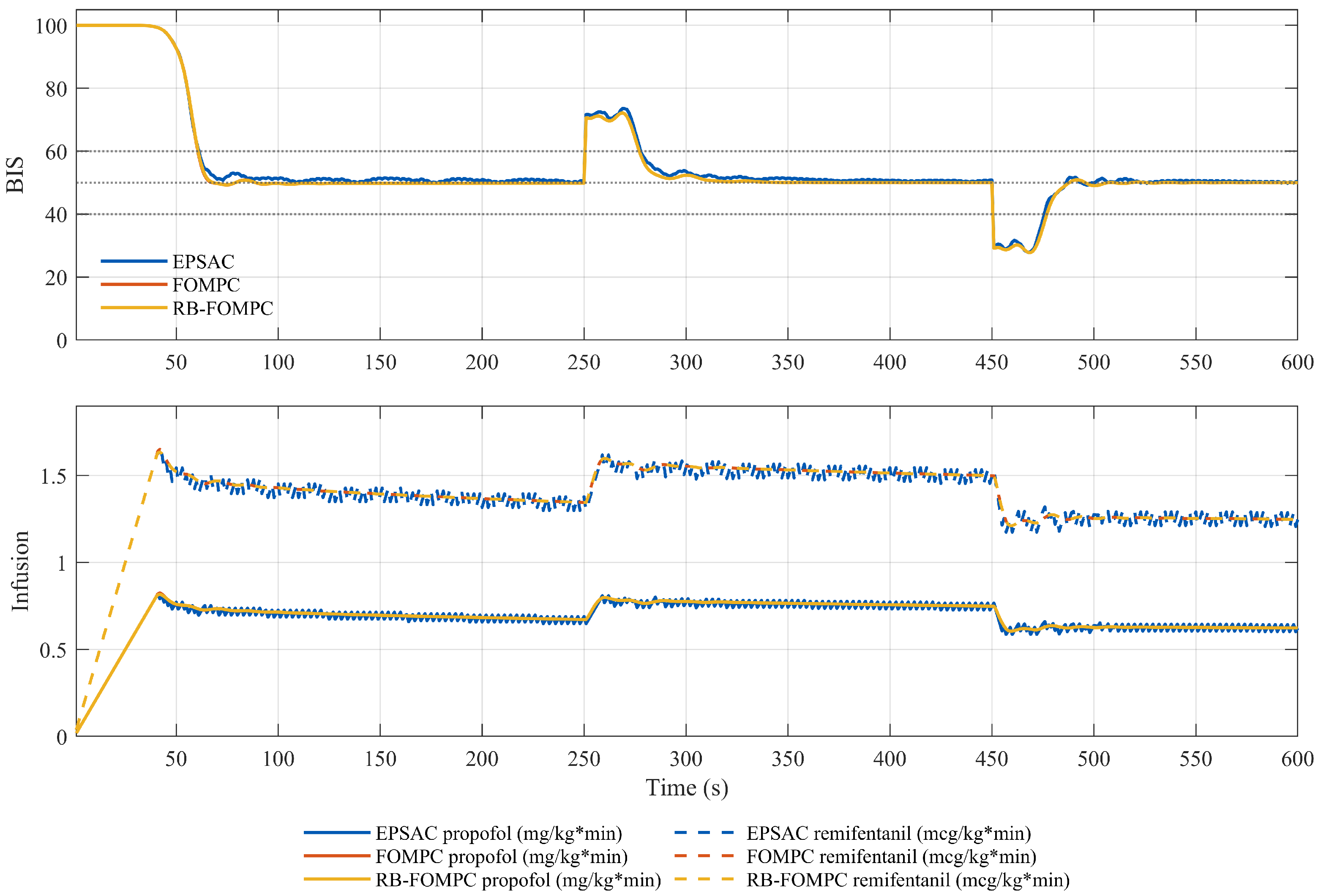
The three control methods were evaluated using the virtual Patient 25, as shown in Figure 6. During the induction phase, the performances of the three methods were similar because the controller was strongly influenced by the system delay and input constraints. After the system reached steady state, FOMPC exhibited improved control performance and smoother control inputs owing to the more flexible shaping of the cost function provided by the fractional-order formulation. No patient-model mismatch was introduced under the current test conditions. The residual-based prediction mechanism was rarely activated, and RB-FOMPC produced almost the same control performance as FOMPC. This similarity is consistent with the design objective of RB-FOMPC, because the residual-based component is expected to remain nearly inactive when the filtered residual does not indicate nominal-model underestimation. This result suggests that the residual-based module did not materially alter FOMPC performance under the nominal Patient 25 simulation.

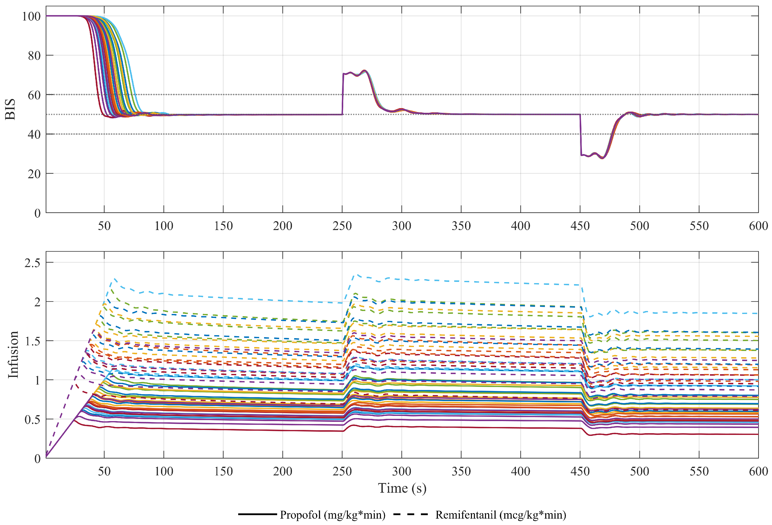
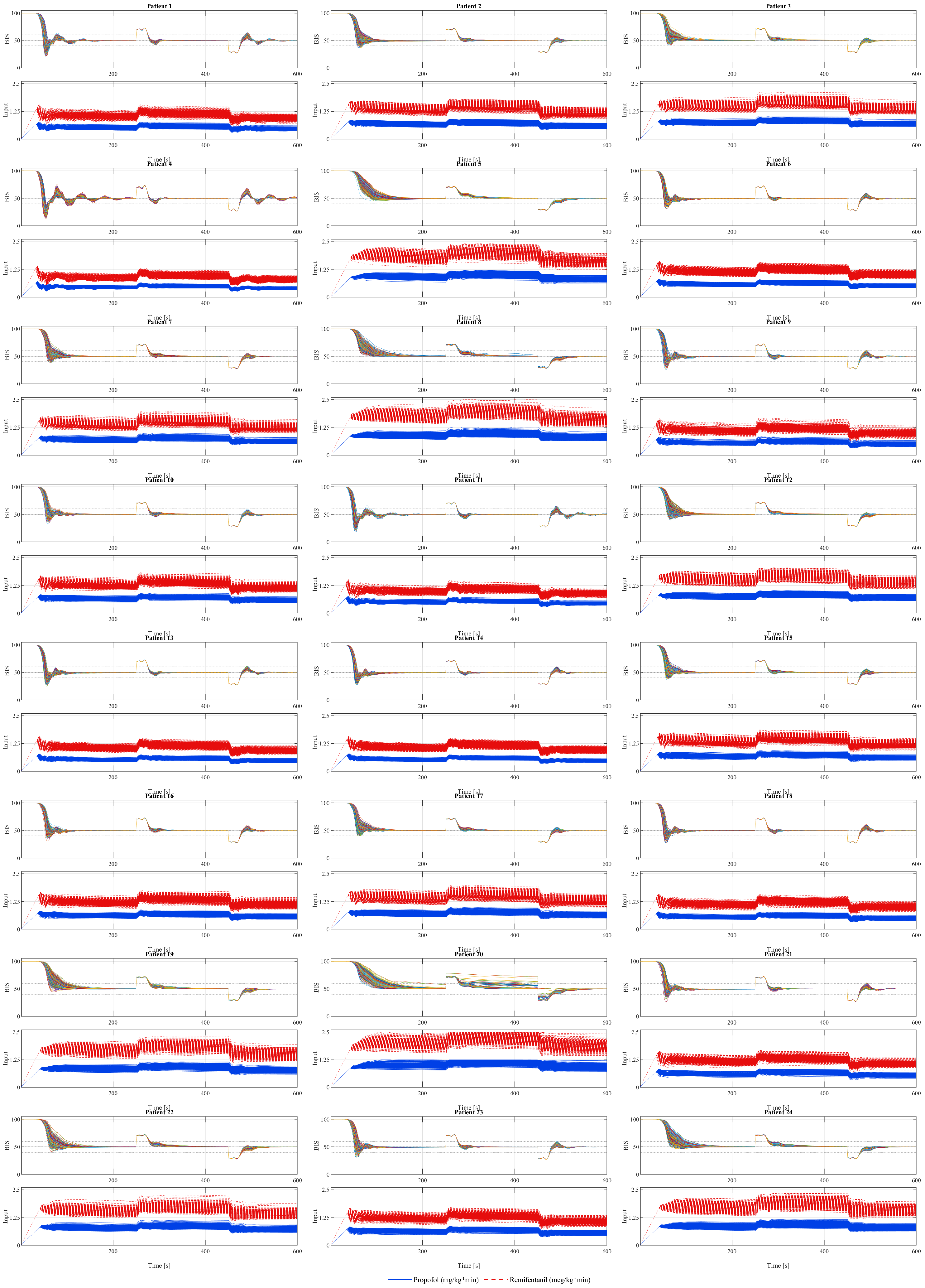
The performance of the RB-FOMPC over the entire patient database is shown in Figure 7. RB-FOMPC maintained stable control performance across all the patient profiles in the database. In each patient, the BIS reached the target range in a relatively short time, and after the surgical stimulation was introduced during the maintenance phase, the BIS returned rapidly to the target range. Across the 25 patient profiles, RB-FOMPC maintained similar convergence patterns without visibly oscillatory infusion inputs.

The results of EPSAC, FOMPC, and RB-FOMPC for the 25 patients, together with their average values, are summarized in

Table 3. Performance comparison among EPSAC, FOMPC, and RB-FOMPC for the 25 patient samples in the database.

	${\mathit{IAE}}_{\mathbf{ind}}$ ($\times {10}^3$)			${\mathit{IAE}}_{\mathbf{mat}}$ ($\times {10}^3$)			BIS-NADIR
Index	EPSAC	FOMPC	RB-FOMPC	EPSAC	FOMPC	RB-FOMPC	EPSAC	FOMPC	RB-FOMPC
1	2.51	2.39	2.39	1.50	1.23	1.23	50.32	49.11	49.08
2	2.88	2.80	2.80	1.42	1.22	1.22	51.06	49.30	49.35
3	2.94	2.86	2.87	1.39	1.22	1.22	51.18	49.56	49.54
4	2.37	2.24	2.24	1.59	1.24	1.24	51.95	48.24	48.26
5	3.41	3.35	3.35	1.40	1.24	1.24	51.46	49.72	49.75
6	2.63	2.54	2.55	1.52	1.23	1.23	51.07	48.92	48.94
7	2.24	2.11	2.11	1.65	1.23	1.23	51.77	48.47	48.48
8	3.26	3.21	3.21	1.43	1.23	1.23	50.55	49.58	49.61
9	2.61	2.51	2.52	1.48	1.22	1.22	50.40	49.03	49.03
10	2.75	2.67	2.68	1.41	1.22	1.22	51.32	49.33	49.33
11	2.46	2.36	2.36	1.49	1.23	1.23	49.89	48.90	48.86
12	3.00	2.94	2.94	1.49	1.23	1.23	51.51	49.39	49.42
13	2.54	2.45	2.45	1.46	1.23	1.23	51.42	48.86	48.87
14	2.60	2.50	2.50	1.59	1.23	1.23	51.95	48.81	48.86
15	2.82	2.74	2.74	1.43	1.22	1.22	51.20	49.32	49.33
16	2.73	2.64	2.64	1.50	1.25	1.25	51.22	48.61	48.69
17	2.88	2.81	2.81	1.44	1.22	1.22	50.88	49.41	49.43
18	2.63	2.52	2.52	1.46	1.23	1.23	51.73	48.94	48.94
19	3.16	3.10	3.11	1.44	1.23	1.23	50.74	49.50	49.56
20	3.50	3.46	3.46	1.39	1.24	1.24	50.49	49.68	49.73
21	2.68	2.58	2.59	1.43	1.22	1.22	50.67	49.19	49.20
22	3.06	2.99	3.00	1.44	1.22	1.22	50.86	49.44	49.49
23	2.69	2.62	2.62	1.46	1.22	1.22	51.34	49.17	49.19
24	3.20	3.14	3.14	1.43	1.23	1.23	50.83	49.51	49.54
25	2.88	2.80	2.80	1.48	1.22	1.22	50.83	49.29	49.32
Average	2.82	2.73	2.74	1.47	1.23	1.23	51.07	49.17	49.19

. $IA{E}_{\mathrm{ind}}$ denotes the IAE during the induction window, whereas $IA{E}_{\mathrm{mat}}$ denotes the IAE during the maintenance window. $BIS-NADIR$ denotes the minimum BIS value reached after the BIS first enters the target region during the induction phase. As indicated by the data in Table 3, all three methods were affected by the combined influence of system delay and input constraints during induction, resulting in only minor differences in $IA{E}_{\mathrm{ind}}$. During the maintenance phase, where finer control adjustments are required, FOMPC and RB-FOMPC achieved lower $IA{E}_{\mathrm{mat}}$ than EPSAC. Under nominal conditions, RB-FOMPC produced almost the same results as FOMPC, indicating that the residual-based module preserved the nominal performance of the fractional-order controller. The average IAU values were 389.44, 391.75, and 391.74 for EPSAC, FOMPC, and RB-FOMPC, respectively, indicating that the improved maintenance phase tracking performance was not achieved at the cost of a substantial increase in total drug administration.

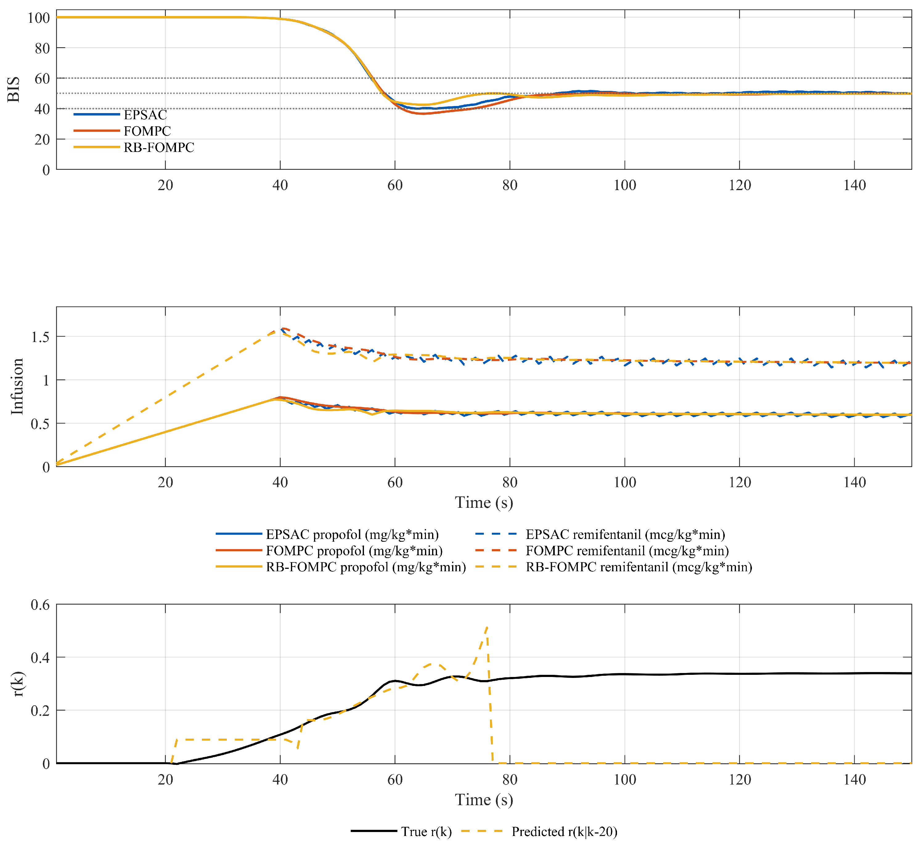
To evaluate the residual-based predictive compensation capability of the proposed RB-FOMPC relative to FOMPC under patient-model mismatch during the induction phase, the intra-patient PK model parameters of Patient 25 were deliberately perturbed. The perturbation strategy was defined by increasing the PK volume parameters $V_1,V_2,V_3$ by 8% and decreasing the clearance parameters $C{l}_1,C{l}_2,C{l}_3$ by 8% for both propofol and remifentanil, while the controller retained the nominal model parameters. The resulting simulation performance is shown in Figure 8. Under the 8% perturbation, RB-FOMPC responded to the positive residual trend by reducing the simulated control input. The BIS nadir was 42.47 with RB-FOMPC and 36.62 with FOMPC, while the time below BIS 40 was 0 and 12 s, respectively. Thus, in this single constructed mismatch scenario, RB-FOMPC was associated with less pronounced BIS undershoot than FOMPC.

These observations support the intended staged behavior of the proposed controller. FOMPC improves the maintenance phase response compared with EPSAC, whereas RB-FOMPC mainly modifies the induction response when a positive residual trend indicates that the nominal model underestimates the actual drug effect. Therefore, the similarity between FOMPC and RB-FOMPC under nominal conditions and their differing responses under the constructed nominal-model-underestimation condition are both consistent with the design objective.

3.3. Robustness Analysis

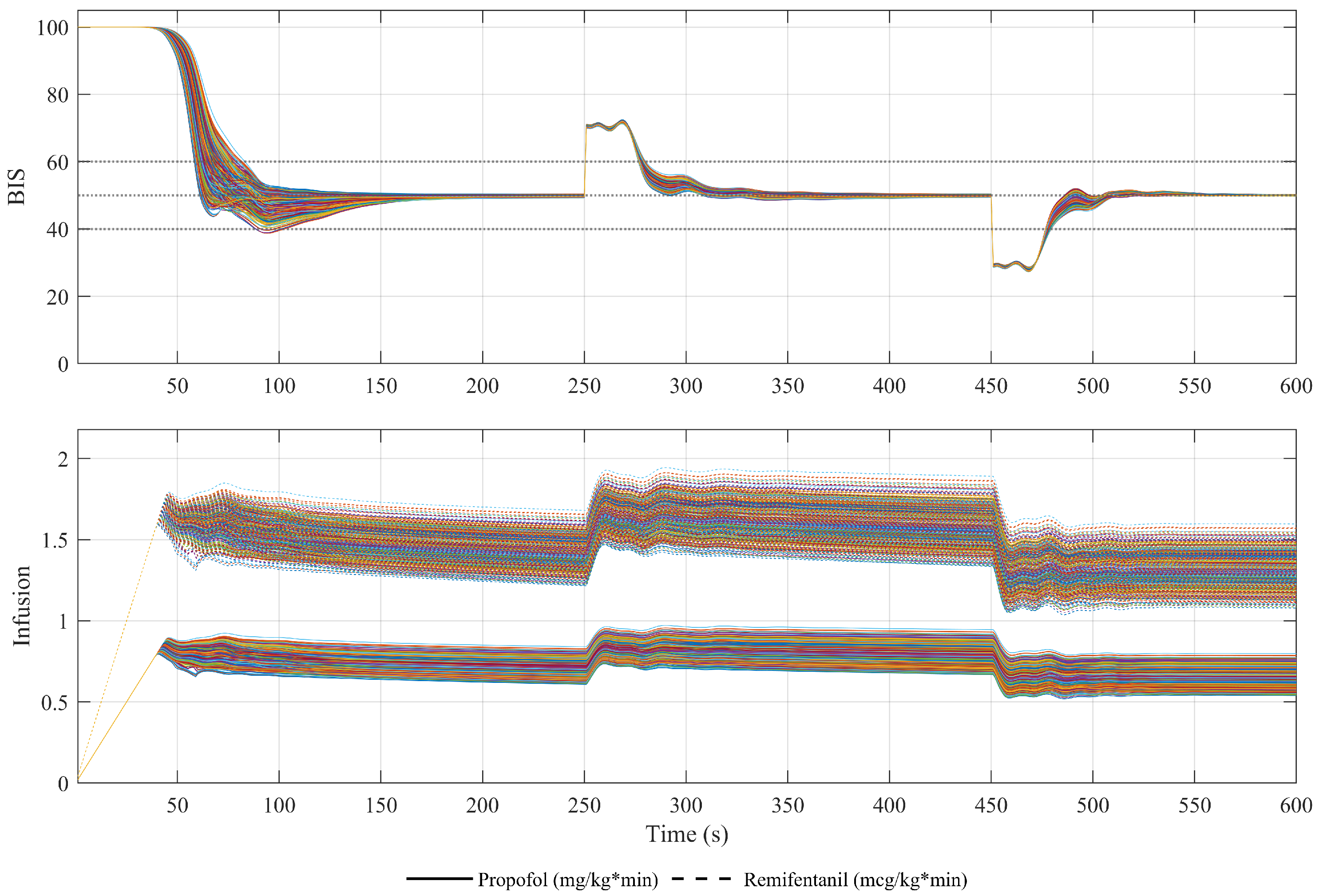
In this section, the Monte Carlo method is used to perform robustness analysis on the controller. The robustness analysis consists of two parts. Inter-patient variability was used to examine whether RB-FOMPC preserves the nominal FOMPC performance across different virtual patients, whereas intra-patient perturbation was used to evaluate the effect of the residual-based module on induction-phase BIS undershoot.

To account for inter-patient variability, this study followed the approach described in Ref. [19] and applied the test to a cohort of 500 simulated patients. The virtual cohort was generated by randomly sampling age, body weight, and height from 18 to 70 years, 50–100 kg, and 150–190 cm, respectively, with sex randomly assigned. In the simulation, the model used in the controller was based on the data of the virtual Patient 25, whereas the patient model adopted the perturbed data. The results of RB-FOMPC under inter-patient variability are shown in Figure 9. All 500 simulated patients were able to reach the target BIS range before surgical stimulation was applied. The results indicate that RB-FOMPC maintained acceptable convergence across inter-patient variability, suggesting that the residual-based mechanism did not visibly destabilize the nominal fractional-order controller.

To better evaluate the controller’s robustness against intra-patient variability, 500 perturbed models were generated for each patient on the basis of that patient’s baseline data. Specifically, for each of the 24 reference patients, the nominal PK parameters were taken as the centers of perturbation. For both propofol and remifentanil, the main PK parameters were perturbed around their nominal values. Each parameter set was randomly perturbed 500 times. For intra-patient variability, age, height, weight, and lean body mass were held fixed for each of the 24 baseline patients. The nominal propofol and remifentanil PK parameters were first calculated using the Schnider and Minto equations, respectively. Multiplicative perturbations were then applied independently to $V_1$, $V_2$, $V_3$, $C{l}_1$, $C{l}_2$, and $C{l}_3$ for each drug according to

$${\theta }^{\prime }=\max \left\{\theta \exp \left(\eta \right),{10}^{-3}\right\},\eta \sim \mathcal{N}\left(0,0.{08}^2\right)$$

(38)

500 perturbations were generated for each patient. The perturbations of the individual PK parameters and those of propofol and remifentanil were generated independently. Thus, 0.08 denotes the prescribed standard deviation of the log-scale perturbation. The final results are shown in Figure 10.

For the Monte Carlo tests, performance metrics are reported as mean ± standard deviation across all variability samples.

Table 4. Average performance metrics of EPSAC, FOMPC, and RB-FOMPC under inter-patient and intra-patient variability. Values are expressed as mean ± standard deviation.

	${\mathit{IAE}}_{\mathbf{ind}}$ ($\times {10}^3$)			${\mathit{IAE}}_{\mathbf{mat}}$ ($\times {10}^3$)			BIS-NADIR			${\mathit{T}}_{\mathbf{BIS}<40}^{\mathbf{ind}}$ (s)
Variability Type	EPSAC	FOMPC	RB-FOMPC	EPSAC	FOMPC	RB-FOMPC	EPSAC	FOMPC	RB-FOMPC	EPSAC	FOMPC	RB-FOMPC
Inter-patient
$(n=500)$	$3.16\pm 0.18$	$3.17\pm 0.19$	$3.17\pm 0.19$	$1.57\pm 0.12$	$1.40\pm 0.09$	$1.40\pm 0.09$	$49.44\pm 2.55$	$48.36\pm 2.68$	$48.36\pm 2.67$	$0.00\pm 0.00$	$0.11\pm 1.10$	$0.11\pm 1.10$
Intra-patient
$(n=\mathrm{12,000})$	$3.13\pm 0.46$	$3.13\pm 0.42$	$2.98\pm 0.44$	$1.55\pm 0.26$	$1.40\pm 0.26$	$1.40\pm 0.25$	$41.80\pm 13.06$	$39.81\pm 13.56$	$44.35\pm 9.51$	$6.87\pm 9.95$	$8.47\pm 11.08$	$2.72\pm 5.85$

Note: $T_{\mathrm{BIS}<40}^{\mathrm{ind}}$ denotes the duration for which the BIS remains below 40 during the induction phase.

presents the performance of the EPSAC, FOMPC, and RB-FOMPC methods on the same set of variability samples, which is consistent with the results of the previous comparative simulations. These results indicate that RB-FOMPC maintained performance close to FOMPC under inter-patient variability, while providing improved safety-related BIS metrics mainly under PK perturbations associated with positive filtered residuals. In particular, RB-FOMPC increased the mean BIS-NADIR and reduced the duration of BIS below 40 compared with FOMPC, suggesting that the residual-based module mainly improves BIS undershoot-related performance under the evaluated patient-centered model perturbations.

Paired analysis of the inter-patient simulations showed that FOMPC reduced the maintenance-phase IAE relative to EPSAC by 167.72, with a 95% confidence interval of 160.09–175.23 and an adjusted $p<0.001$. The corresponding increase in IAU was 2.78, representing approximately 0.65% of the EPSAC mean. Thus, the maintenance-phase improvement was accompanied by only a small increase in cumulative simulated input.

Analysis of Positive Residual Cases

This subset was defined according to the pre-specified activation condition of the compensation mechanism. Since the proposed residual-based compensation is designed as a one-sided residual-correction mechanism, its effect may be diluted when all intra-patient samples are averaged together. Therefore, an additional analysis was conducted by extracting the intra-patient variability samples with positive filtered effect-site residuals from Patients 1–24. These samples correspond to cases in which the nominal model underestimates the actual equivalent propofol-related drug effect, which is the main situation targeted by RB-FOMPC.

As shown in

Table 5. Average performance metrics of EPSAC, FOMPC, and RB-FOMPC for intra-patient variability samples with positive filtered effect-site residuals from Patients 1–24. Values are expressed as mean ± standard deviation.

	${\mathit{IAE}}_{\mathbf{ind}}$ ($\times {10}^3$)			${\mathit{IAE}}_{\mathbf{mat}}$ ($\times {10}^3$)			BIS-NADIR			${\mathit{T}}_{\mathbf{BIS}<40}^{\mathbf{ind}}$ (s)
Subset	EPSAC	FOMPC	RB-FOMPC	EPSAC	FOMPC	RB-FOMPC	EPSAC	FOMPC	RB-FOMPC	EPSAC	FOMPC	RB-FOMPC
Positive filtered residual
($n=7455$)	$2.90\pm 0.27$	$2.96\pm 0.29$	$2.72\pm 0.13$	$1.44\pm 0.17$	$1.33\pm 0.22$	$1.32\pm 0.19$	$33.97\pm 11.44$	$31.35\pm 11.26$	$38.94\pm 8.69$	$11.51\pm 10.61$	$14.15\pm 11.19$	$4.57\pm 6.99$

, the benefit of RB-FOMPC became more pronounced after restricting the analysis to positive-residual samples. Compared with FOMPC, RB-FOMPC reduced $IA{E}_{\mathrm{ind}}$ from $2.96\times {10}^3$ to $2.72\times {10}^3$, increased the BIS-NADIR from 31.35 to 38.94, and reduced $T_{\mathrm{BIS}<40}^{\mathrm{ind}}$ from 14.15 s to 4.57 s. The reduction in the duration below BIS 40 was approximately 67.7%, indicating a substantial decrease in excessive BIS undershoot during induction.

When each contributing virtual patient was weighted equally, RB-FOMPC reduced the induction-phase IAE by 177.81 relative to FOMPC, with a 95% confidence interval of 96.89–271.17. It also increased the BIS nadir by 5.56 and reduced the duration below BIS 40 by 7.00 s, with corresponding 95% confidence intervals of 3.74–7.39 and 4.65–9.36 s, respectively. All three comparisons remained significant after Holm adjustment ($p<0.001$).

Meanwhile, the IAU remained almost unchanged, decreasing slightly from 330.56 to 330.03. The maintenance phase IAE also remained close to that of FOMPC, changing from $1.33\times {10}^3$ to $1.32\times {10}^3$. These results indicate that the residual-based compensation mainly improves induction-phase BIS undershoot-related metrics in the positive residual subset, without increasing the cumulative simulated input or compromising the maintenance phase regulation performance.

Compared with the full intra-patient variability results, this positive-residual subset provides a less diluted evaluation of the residual-based mechanism. The improvement is concentrated in the metrics directly related to excessive anesthesia depth, namely BIS-NADIR and $T_{\mathrm{BIS}<40}^{\mathrm{ind}}$, which is consistent with the design objective of RB-FOMPC. Therefore, the results indicate that the proposed residual compensation acts primarily when the nominal model underestimates the actual drug effect and provides an additional reduction in severe BIS undershoot within the evaluated subset.

3.4. Computational Time

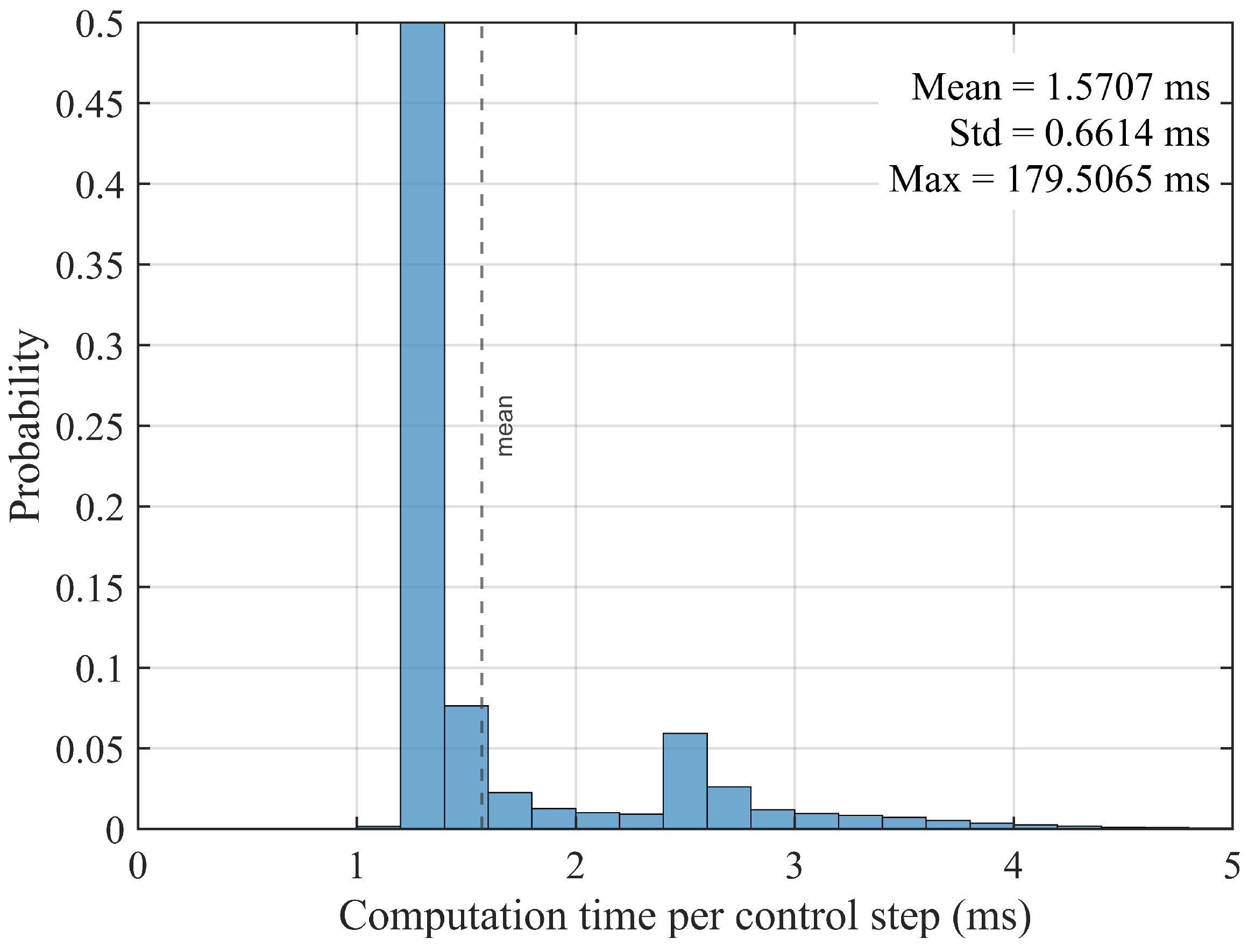
The computational efficiency of the proposed RB-FOMPC strategy was evaluated by solving the underlying MPC optimization problem using quadratic programming (QP) at each sampling instant. The histogram of the solution time at each step during the robustness verification simulation is shown in Figure 11. The measured average computation time per control step was 1.57 ms, which is well below the typical sampling time used in anesthesia control applications and therefore indicates computational tractability in the tested simulation environment. The worst-case computation time was 179.5 ms. However, this value was still shorter than the sampling time, indicating that the proposed method remained compatible with the selected 1 s sampling period in the tested simulation environment. The computational burden is further reduced by the use of a time-invariant prediction matrix G, which is computed offline, and by handling nonlinearities through an external predictor without modifying the linear QP structure. These features allow the controller to maintain low computational complexity while preserving high control performance.

4. Discussion

The simulation results show that the proposed RB-FOMPC strategy improves automated propofol–remifentanil co-administration within the EPSAC framework. The results also indicate two distinct sources of improvement. The fractional-order cost function mainly enhances maintenance phase regulation by redistributing the tracking-error and input-increment penalties over the prediction and control horizons. Compared with EPSAC, FOMPC reduces the maintenance phase tracking error while only slightly changing the IAU.

The residual-based compensation mainly contributes to safety-related BIS metrics during induction under patient-model mismatch. Under nominal conditions, RB-FOMPC remains close to FOMPC, indicating that the residual compensation does not unnecessarily alter the nominal controller behavior. Under intra-patient perturbations, especially when the nominal model underestimates the actual drug effect, RB-FOMPC increases the BIS-NADIR and reduces the duration of BIS below 40. This indicates that the residual-based module acts primarily as a one-sided residual-correction mechanism against excessive BIS undershoot.

The external predictor and residual correction structure also help preserve computational efficiency. The inverse Hill mapping handles the nonlinear BIS-drug effect relationship outside the online optimization problem, while the Kalman filter attenuates fluctuations in the reconstructed residual. The dynamic residual predictor then extrapolates the filtered mismatch over the prediction horizon. As a result, the proposed method reduced undershoot metrics within the tested perturbation envelope in the targeted positive-residual cases without changing the linear QP structure of EPSAC.

The robustness analysis supports these observations. Under inter-patient variability, RB-FOMPC maintained performance close to that of FOMPC, and no clear performance loss attributable to the residual-based module was observed in the tested trajectories. Under intra-patient variability, RB-FOMPC showed clearer improvements in BIS undershoot-related metrics during induction, particularly in positive-residual cases. However, these results are still simulation-based and should not be interpreted as direct clinical evidence.

The computation-time results further indicate that the proposed method is feasible for real-time implementation within the 1 s sampling period. Since the prediction matrices are computed offline and the residual-based module does not alter the linear optimization structure, the average and worst-case computation times remain below the sampling interval.

Limitations of This Study

Several limitations should be acknowledged. First, the proposed controller was evaluated only in simulation using PK/PD-based virtual-patient models. Although Monte Carlo analysis considered inter- and intra-patient variability, the selected perturbations represent numerical uncertainty envelopes and cannot fully reproduce clinical variability. The simulations did not include additional stochastic BIS measurement noise, induction-phase disturbances, variable sensor delays, actuator dynamics, or broader structural pharmacodynamic uncertainty. In addition, the simulation protocol did not include discontinuation of the drug infusions or a recovery phase. Second, BIS was used as the sole controlled physiological variable, whereas practical anesthesia management also requires consideration of hemodynamic and analgesia-related indicators. Third, the fixed propofol–remifentanil infusion ratio improves input smoothness but limits independent optimization of hypnosis and analgesia. Future work will therefore focus on more comprehensive uncertainty and disturbance analysis, hardware-in-the-loop testing, retrospective clinical-data validation, and subsequent animal and clinical studies.

5. Conclusions

This paper proposed an RB-FOMPC strategy for automated propofol–remifentanil co-administration within the EPSAC framework. The fractional-order cost function improved the flexibility of the predictive control objective and mainly enhanced maintenance phase regulation, while the dynamic residual-based predictive compensation improved induction phase safety-related metrics under conditions in which the nominal model underestimated the BIS-derived equivalent propofol-related effect. Simulation results showed that, under nominal conditions, RB-FOMPC preserved the performance of FOMPC without introducing unnecessary compensation. Under intra-patient variability, RB-FOMPC improved induction-phase safety-related BIS metrics by increasing the BIS-NADIR and reducing the duration of BIS below 40 compared with FOMPC, while maintaining similar maintenance phase tracking performance. The positive-residual subset analysis further indicated that the benefit of RB-FOMPC was concentrated in cases where the nominal model underestimated the actual drug effect. In addition, the computation-time results indicated that the proposed method was computationally feasible within the selected sampling period in the simulation environment. Overall, the simulations indicate that FOMPC improves maintenance-phase regulation, while the residual-based extension provides a simulation-based induction-undershoot mitigation mechanism under the evaluated nominal-model-underestimation conditions.

References

1. Laferrière-Langlois, P.; Morisson, L.; Jeffries, S.; Duclos, C.; Espitalier, F.; Richebé, P. Depth of anesthesia and nociception monitoring: Current state and vision for 2050. Anesth. Analg. 2024, 138, 295–307. [Google Scholar] [CrossRef] [Scilit]
2. Felippe, V.A.; Dias, H.S.; da Hora, D.A.B.; Wegner, B.F.M.; Wegner, G.R.M.; González, G.L.; Piredda, G.V.; Bezerra, F.J.L.; Bersot, C.D.A.; Lessa, M.A. Closed-loop systems for automated hypnotic drug delivery during general anaesthesia: A systematic review and meta-analysis. Br. J. Anaesth. 2026, 136, 1811–1821. [Google Scholar] [CrossRef] [Scilit] [PubMed]
3. Copot, D. Automated Drug Delivery in Anesthesia; Academic Press: London, UK, 2020. [Google Scholar]
4. van Heusden, K.; Ansermino, J.M.; Dumont, G.A. Robust MISO control of propofol-remifentanil anesthesia guided by the NeuroSENSE monitor. IEEE Trans. Control Syst. Technol. 2018, 26, 1758–1770. [Google Scholar] [CrossRef] [Scilit]
5. Birs, I.; Muresan, C.; Ghita, M.; Ghita, M.; Nascu, I.; Ionescu, C. Event-Based Fractional Order MIMO Control for Hemodynamic Stabilization During General Anesthesia. In Proceedings of the 2023 IEEE International Conference on Systems, Man, and Cybernetics (SMC); IEEE: Piscataway, NJ, USA, 2023; pp. 1295–1300. [Google Scholar] [CrossRef] [Scilit]
6. Liu, N.; Chazot, T.; Hamada, S.; Landais, A.; Boichut, N.; Dussaussoy, C.; Trillat, B.; Beydon, L.; Samain, E.; Sessler, D.I.; et al. Closed-loop coadministration of propofol and remifentanil guided by bispectral index: A randomized multicenter study. Anesth. Analg. 2011, 112, 546–557. [Google Scholar] [CrossRef] [Scilit] [PubMed]
7. Ionescu, C.M.; Neckebroek, M.; Ghita, M.; Copot, D. An open source patient simulator for design and evaluation of computer based multiple drug dosing control for anesthetic and hemodynamic variables. IEEE Access 2021, 9, 8680–8694. [Google Scholar] [CrossRef] [Scilit]
8. Gan, V.; Dumont, G.A.; Mitchell, I. Benchmark Problem: A PK/PD Model and Safety Constraints for Anesthesia Delivery. In ARCH14-15. 1st and 2nd International Workshop on Applied Verification for Continuous and Hybrid Systems; EPiC Series in Computing; EasyChair: Stockport, UK, 2015; Volume 34, pp. 1–8. [Google Scholar] [CrossRef] [Scilit]
9. Krieger, A.; Panoskaltsis, N.; Mantalaris, A.; Georgiadis, M.C.; Pistikopoulos, E.N. Modeling and analysis of individualized pharmacokinetics and pharmacodynamics for volatile anesthesia. IEEE Trans. Biomed. Eng. 2014, 61, 25–34. [Google Scholar] [CrossRef] [Scilit] [PubMed]
10. Eleveld, D.J.; Colin, P.; Absalom, A.R.; Struys, M.M. Pharmacokinetic–pharmacodynamic model for propofol for broad application in anaesthesia and sedation. Br. J. Anaesth. 2018, 120, 942–959. [Google Scholar] [CrossRef] [Scilit] [PubMed]
11. Padula, F.; Ionescu, C.; Latronico, N.; Paltenghi, M.; Visioli, A.; Vivacqua, G. Optimized PID control of depth of hypnosis in anesthesia. Comput. Methods Programs Biomed. 2017, 144, 21–35. [Google Scholar] [CrossRef] [Scilit] [PubMed]
12. Schiavo, M.; Padula, F.; Latronico, N.; Merigo, L.; Paltenghi, M.; Visioli, A. Performance evaluation of an optimized PID controller for propofol and remifentanil coadministration in general anesthesia. IFAC J. Syst. Control 2021, 15, 100121. [Google Scholar] [CrossRef] [Scilit]
13. Laurini, M.; Llopis, T.; Naz, N.; Consolini, L.; Milanesi, M.; Schiavo, M.; Visioli, A. Optimized Feedforward Control for the Co-administration of Propofol and Remifentanil for Induction of Hypnosis in General Anesthesia. IEEE Control Syst. Lett. 2025, 9, 745–750. [Google Scholar] [CrossRef] [Scilit]
14. Raymond, M.; Moussa, K.; Fiacchini, M.; Lauber, J. MPC-Based Anesthesiologists Imitating Control of Propofol and Remifentanil during Anesthesia Maintenance. In Proceedings of the 2025 29th International Conference on System Theory, Control and Computing (ICSTCC); IEEE: Piscataway, NJ, USA, 2025; pp. 588–594. [Google Scholar] [CrossRef] [Scilit]
15. Eskandari, N.; van Heusden, K.; Dumont, G.A. Extended habituating model predictive control of propofol and remifentanil anesthesia. Biomed. Signal Process. Control 2020, 55, 101656. [Google Scholar] [CrossRef] [Scilit]
16. Pawlowski, A.; Schiavo, M.; Latronico, N.; Paltenghi, M.; Visioli, A. MPC for propofol anesthesia: The noise issue. In Proceedings of the 2022 IEEE Conference on Control Technology and Applications (CCTA); IEEE: Piscataway, NJ, USA, 2022; pp. 1087–1092. [Google Scholar] [CrossRef] [Scilit]
17. Pawłowski, A.; Schiavo, M.; Latronico, N.; Paltenghi, M.; Visioli, A. Linear MPC for anesthesia process with external predictor. Comput. Chem. Eng. 2022, 161, 107747. [Google Scholar] [CrossRef] [Scilit]
18. Pawłowski, A.; Schiavo, M.; Latronico, N.; Paltenghi, M.; Visioli, A. Drug co-administration in anesthesia using event-based MPC. Int. J. Robust Nonlinear Control 2025, 35, 4020–4042. [Google Scholar] [CrossRef] [Scilit]
19. Pawłowski, A.; Schiavo, M.; Latronico, N.; Paltenghi, M.; Visioli, A. Event-based MPC for propofol administration in anesthesia. Comput. Methods Programs Biomed. 2023, 229, 107289. [Google Scholar] [CrossRef] [Scilit] [PubMed]
20. Li, W.; Yan, S.; Shi, L.; Yue, J.; Shi, M.; Lin, B.; Qin, K. Multiagent Consensus Tracking Control Over Asynchronous Cooperation–Competition Networks. IEEE Trans. Cybern. 2025, 55, 4347–4360. [Google Scholar] [CrossRef] [Scilit] [PubMed]
21. Nino, J.; De Keyser, R.; Syafiie, S.; Ionescu, C.; Struys, M. EPSAC-controlled anesthesia with online gain adaptation. Int. J. Adapt. Control Signal Process. 2009, 23, 455–471. [Google Scholar] [CrossRef] [Scilit]
22. Zhao, S.; Mu, J.; Liu, H.; Sun, Y.; Cajo, R. Heading control of USV based on fractional-order model predictive control. Ocean Eng. 2025, 322, 120476. [Google Scholar] [CrossRef] [Scilit]
23. Zhao, S.; Wang, S.; Cajo, R.; Ren, W.; Li, B. Power tracking control of marine boiler-turbine system based on fractional order model predictive control algorithm. J. Mar. Sci. Eng. 2022, 10, 1307. [Google Scholar] [CrossRef] [Scilit]
24. Cajo, R.; Zhao, S.; Plaza, D.; De Keyser, R.; Ionescu, C. A Fractional Order Predictive Control for Trajectory Tracking of the AR.Drone Quadrotor. In Proceedings of the CONTROLO 2020; Gonçalves, J.A., Braz-César, M., Coelho, J.P., Eds.; Springer International Publishing: Cham, Switzerland, 2020; pp. 528–537. [Google Scholar] [CrossRef] [Scilit]
25. Cajo, R.; Mac, T.T.; Plaza, D.; Copot, C.; De Keyser, R.; Ionescu, C. A survey on fractional order control techniques for unmanned aerial and ground vehicles. IEEE Access 2019, 7, 66864–66878. [Google Scholar] [CrossRef] [Scilit]
26. Navarro-Guerrero, G.; Tang, Y. Fractional-order closed-loop model reference adaptive control for anesthesia. Algorithms 2018, 11, 106. [Google Scholar] [CrossRef] [Scilit]
27. Dulf, E.H.; Pintea, P.A.; Muresan, C.I. Anesthesia Control Using Fractional Order Controller. In Proceedings of the 2024 18th International Conference on Control, Automation, Robotics and Vision (ICARCV); IEEE: Piscataway, NJ, USA, 2024; pp. 1178–1181. [Google Scholar] [CrossRef] [Scilit]
28. Milanesi, M.; Consolini, L.; Di Credico, G.; Latronico, N.; Laurini, M.; Paltenghi, M.; Schiavo, M.; Visioli, A. Patient-Specific MPC for Improved Robustness in Anesthesia. Commun. Nonlinear Sci. Numer. Simul. 2026, 162, 110210. [Google Scholar] [CrossRef] [Scilit]
29. Mihai, M.; Birs, I.; Hegedus, E.; Ynineb, A.; Copot, D.; De Keyser, R.; Ionescu, C.M.; Ladaci, S.; Muresan, C.I.; Neckebroek, M. Online and personalised control of the depth of hypnosis during induction using fractional order PID. J. Adv. Res. 2025, 78, 777–789. [Google Scholar] [CrossRef] [Scilit] [PubMed]
30. Absalom, A.; Struys, M.M. An overview of TCI & TIVA; Lannoo Meulenhoff-Belgium: Gent, Belgium, 2019. [Google Scholar]
31. Minto, C.F.; Schnider, T.W.; Egan, T.D.; Youngs, E.; Lemmens, H.J.; Gambus, P.L.; Billard, V.; Hoke, J.F.; Moore, K.H.; Hermann, D.J.; et al. Influence of age and gender on the pharmacokinetics and pharmacodynamics of remifentanil: I. Model development. Anesthesiology 1997, 86, 10–23. [Google Scholar] [CrossRef] [Scilit] [PubMed]
32. Goutelle, S.; Maurin, M.; Rougier, F.; Barbaut, X.; Bourguignon, L.; Ducher, M.; Maire, P. The Hill equation: A review of its capabilities in pharmacological modelling. Fundam. Clin. Pharmacol. 2008, 22, 633–648. [Google Scholar] [CrossRef] [Scilit] [PubMed]
33. Minto, C.F.; Schnider, T.W.; Shafer, S.L. Pharmacokinetics and pharmacodynamics of remifentanil: II. Model application. Anesthesiology 1997, 86, 24–33. [Google Scholar] [CrossRef] [Scilit] [PubMed]
34. Pawłowski, A.; Schiavo, M.; Latronico, N.; Paltenghi, M.; Visioli, A. Model predictive control using MISO approach for drug co-administration in anesthesia. J. Process Control 2022, 117, 98–111. [Google Scholar] [CrossRef] [Scilit]
35. Merigo, L.; Padula, F.; Latronico, N.; Paltenghi, M.; Visioli, A. Event-based control tuning of propofol and remifentanil coadministration for general anaesthesia. IET Control Theory Appl. 2020, 14, 2995–3008. [Google Scholar] [CrossRef] [Scilit]
36. West, N.; Van Heusden, K.; Görges, M.; Brodie, S.; Rollinson, A.; Petersen, C.L.; Dumont, G.A.; Ansermino, J.M.; Merchant, R.N. Design and evaluation of a closed-loop anesthesia system with robust control and safety system. Anesth. Analg. 2018, 127, 883–894. [Google Scholar] [CrossRef] [Scilit] [PubMed]
37. Schiavo, M.; Paltenghi, M.; Visioli, A.; Latronico, N. Clinical performance of a bispectral index controlled closed-loop administration system for simultaneous administration of propofol and remifentanil. Anesth. Analg. 2025, 140, 1236–1238. [Google Scholar] [CrossRef] [Scilit] [PubMed]
38. De Keyser, R. Model based predictive control for linear systems. In Control Systems, Robotics and Automation; EOLSS Publishers/UNESCO: Oxford, UK, 2003; Volume XI, pp. 24–58. [Google Scholar]
39. Castano, J.A.; Hernandez, A.; Li, Z.; Tsagarakis, N.G.; Caldwell, D.G.; De Keyser, R. Enhancing the robustness of the EPSAC predictive control using a Singular Value Decomposition approach. Robot. Auton. Syst. 2015, 74, 283–295. [Google Scholar] [CrossRef] [Scilit]
40. Copot, D.; Ionescu, C. Models for nociception stimulation and memory effects in awake and aware healthy individuals. IEEE Trans. Biomed. Eng. 2019, 66, 718–726. [Google Scholar] [CrossRef] [Scilit] [PubMed]
41. Ionescu, C.; Lopes, A.; Copot, D.; Machado, J.T.; Bates, J.H. The role of fractional calculus in modeling biological phenomena: A review. Commun. Nonlinear Sci. Numer. Simul. 2017, 51, 141–159. [Google Scholar] [CrossRef] [Scilit]
Figure 1. Pharmacokinetic model compartment scheme for one drug.
Mathematics 14 02979 g001
Figure 2. PK/PD models for drug co-administration in patients.
Mathematics 14 02979 g002
Figure 3. PK/PD model for drug co-administration with an added infusion-ratio constraint.
Mathematics 14 02979 g003
Figure 4. FOMPC framework integrated with an external predictor.
Mathematics 14 02979 g004
Figure 5. RIAE results of FOMPC in anesthesia depth control.
Mathematics 14 02979 g005
Figure 6. Comparison of BIS responses and infusion inputs obtained using EPSAC, FOMPC, and RB-FOMPC under the nominal Patient 25 condition.
Mathematics 14 02979 g006
Figure 7. The control performance of RB-FOMPC on the 25 patient profiles in the database.
Mathematics 14 02979 g007
Figure 8. Performance of the three control methods during the induction phase under patient-model mismatch.
Mathematics 14 02979 g008
Figure 9. The control performance of RB-FOMPC on 500 inter-patient variability samples generated from virtual patients in the database.
Mathematics 14 02979 g009
Figure 10. The control performance of RB-FOMPC on 12,000 intra-patient variability samples derived from 24 patients in the database.
Mathematics 14 02979 g010
Figure 11. Distribution of solve time at each control step.
Mathematics 14 02979 g011