Multi-Agent Reinforcement Learning Game Model for Market Economic Equilibrium Regulation

Abstract

Market equilibrium regulation constitutes a dynamic decision-making problem on complex networks, where strategic firms, consumers, platforms, and regulators interact under uncertain demand, delayed price information, and networked spillovers. Although existing multi-agent reinforcement learning (MARL) methods succeed at decentralized adaptation, they typically maximize private rewards without encoding an explicit equilibrium residual or a rigorous link to market clearing. We introduce an Equilibrium-Residual Mirror Multi-Agent Reinforcement Learning (ERM-MARL) framework for regulating market equilibria. The framework formulates a regulated Markov potential game: agents learn pricing, production, and risk-control policies while a dual regulation layer penalizes violations of market clearing, price volatility, and network risk. An equilibrium-residual shaping mechanism aligns each agent’s policy gradient with a global regulation potential. The analysis establishes existence of equilibrium, uniqueness under strong monotonicity, bounded dual stability, and almost-sure convergence of the stochastic mirror actor–critic recursion. Simulation experiments on networked markets demonstrate faster equilibrium-residual decay, higher welfare, lower price volatility, and greater robustness compared with representative MARL and game-learning baselines.

1. Introduction

Regulating market equilibria involves steering many self-interested participants toward stable clearing, acceptable welfare, and bounded systemic risk [1,2]. Far from a static price-finding exercise, it is a dynamic, networked, and strategic control problem: firms adjust production, platforms change fees, consumers respond to prices, and regulators impose taxes, subsidies, or risk limits. Such challenges arise in electricity markets [3], digital platforms [4], mobility markets [5], supply chains [6], and financial liquidity systems [7]. Recent multi-agent reinforcement learning (MARL) research confirms that decentralized agents can learn adaptive policies in large games, communication systems, and market-like environments [8,9,10]. However, equilibrium regulation demands more than high empirical return; it requires a mathematically traceable connection between learning dynamics, market-clearing constraints, and economic stability [11].

Several useful components have emerged in the literature. Transformer-based and graph-based MARL architectures improve coordination under heterogeneous interactions [12]. Task-offloading and aggregative-game research show that distributed learning and distributed Nash seeking can operate over time-varying networks [13,14]. Differential graphical games and mean-field control provide tools for adversarial inputs, large populations, and sticky price dynamics, while variational-inequality models have become important for analyzing trade-network equilibria during crises [15,16]. Those developments indicate that reinforcement learning, games, and network dynamics are converging toward a unified decision-making framework [17]. Broader theoretical work has also clarified stochastic-game foundations, sequence modeling, equilibrium selection, and evolutionary perspectives on MARL [18].

Despite this progress, three limitations stand out. First, most MARL algorithms optimize local rewards and treat equilibrium as an external metric; consequently, the learning signal can be misaligned with clearing, volatility, and systemic-risk constraints. Second, bidding studies for electricity and resource markets often assume domain-specific bid structures or rely on centralized market simulators, leaving the regulator’s dynamic role implicit. Third, advances in financial market-making, Stackelberg Markov games, and mean-field learning have refined strategic modeling, yet they rarely supply a single Lyapunov-type potential that simultaneously covers policy improvement, dual feasibility, and networked equilibrium residuals [19,20]. Those gaps call for a new MARL game model in which the equilibrium residual is built into the learning objective rather than used as a post hoc diagnostic [21]. Related work on energy-market and supply-network systems further highlights that bidding, charging, inventory, and routing decisions must be coupled with equilibrium-aware adaptation [22,23].

We adopt a regulated Markov potential-game perspective [24]. Its key advantage is that individual learning can be tied to a global potential while preserving decentralized execution. The proposed model combines mean-field approximation, mirror-descent policy updates [25], dual regulation prices [26], and equilibrium-residual reward shaping [27]. Compared with pure policy-gradient MARL [28], this design embeds economic structure into the learning process; compared with exact game solvers, it scales to nonlinear stochastic markets with incomplete local observations; compared with static mechanism design, it adapts to shocks and evolving network topology. Recent work on continuous mean-field games, network-slicing games, differential-game optimization, and transmission expansion reinforces the need for such dynamic, data-driven, and network-aware regulation. Likewise, MARL advances in urban air mobility, traffic control, roundabout coordination, and container-terminal scheduling reveal the same need for scalable decentralized decision-making on networks.

The proposed framework is positioned at the intersection, rather than the union, of three lines of work. Markov potential-game methods provide an equilibrium structure, but they do not themselves enforce market-clearing inequalities or quantify complementary slackness along sampled trajectories. Constrained or primal–dual reinforcement learning introduces penalties and multipliers, yet it commonly treats the constraint signal as an external safety device and does not establish that decentralized policy updates follow a common market potential. Deterministic variational-inequality solvers, in turn, usually require direct evaluations of the market operator. ERM-MARL differs by using the same normalized residual to shape local advantages, update dual prices, and certify the regulated equilibrium. The consensus critic and mirror geometry make this construction operational under partial local observations and stochastic trajectories.

In this work, we develop ERM-MARL for market equilibrium regulation. The market is modeled as a directed weighted complex network: nodes represent strategic agents and edges capture transaction, substitution, and information dependencies. Each agent chooses a mixed action vector comprising price markup, production adjustment, inventory release, and risk exposure. A regulator monitors aggregate clearing residuals and updates dual prices. The learning objective is a penalized regulation potential that rewards welfare improvement while discouraging price dispersion, unmet demand, inventory stress, and systemic-risk amplification. The resulting procedure is an actor–critic algorithm with mirror policy updates and consensus critics.

The main contributions are threefold. First, we formulate a regulated Markov potential game for networked market equilibrium and derive an equilibrium residual that unifies price-clearing, welfare, volatility, and network-risk measures. Second, we design ERM-MARL, a mirror-dual actor–critic algorithm in which reward shaping aligns every agent’s advantage with the global regulation potential. Third, we prove equilibrium existence, uniqueness under strong monotonicity, bounded dual stability, and almost-sure convergence of the proposed stochastic learning recursion. These contributions directly address the theme of dynamic analysis and decision-making in complex networks. The main notation used in this paper is listed in

Table 1. Main symbols and definitions.

Symbol	Definition	Symbol	Definition
$\mathcal{G}=(\mathcal{V},\mathcal{E},W)$	directed market interaction graph	N	number of strategic agents
i	market agent index	t	discrete market period
$s_t$	global market state	$o_{i,t}$	local observation of agent i
$a_{i,t}$	action of agent i	${\pi }_i$	stochastic policy of agent i
$p_{i,t}$	local price decision	$q_{i,t}$	production or supply decision
$d_{i,t}$	realized demand	${\ell }_t$	aggregate clearing residual
${\rho }_t$	network-risk index	${\nu }_t$	price-volatility index
$g(s,a)$	vector market constraint residual	${\lambda }_t$	dual regulation price
$J_i$	discounted return of agent i	$\Phi$	regulated potential function
$A_i^{\pi }$	individual advantage function	$D_{\psi }$	Bregman divergence
${\eta }_t$	actor stepsize	${\beta }_t$	dual stepsize
$\gamma$	discount factor	$\tau$	entropy temperature
${ϵ}_t$	equilibrium-residual norm	${\overline{a}}_t$	mean-field action statistic

.

2. Problem Description and Preliminaries

2.1. Networked Market State

We consider a market with N strategic agents situated on a directed weighted graph $\mathcal{G}=(\mathcal{V},\mathcal{E},W)$, where $\mathcal{V}=\{1,\dots ,N\}$ and each edge weight $w_{ij}\ge 0$ measures the influence of agent j’s action on the local state of agent i. The graph may encode supply-chain exposure, substitution relations, price information, or platform traffic. The global state is

$$s_t={\left[x_{1,t}^{\top },\dots ,x_{N,t}^{\top },z_t^{\top }\right]}^{\top }\in \mathcal{S},$$

(1)

where $x_{i,t}$ collects local price, inventory, backlog, liquidity, and cost information, and $z_t$ captures exogenous demand and macro shocks. Agent i receives the observation

$$o_{i,t}=H_i{s}_t+{\sum }_{j\in {\mathcal{N}}_i}{h}_{ij}\left(x_{j,t}\right)+{\epsilon }_{i,t},$$

(2)

where ${\mathcal{N}}_i=\{j:w_{ij}>0\}$ and ${\epsilon }_{i,t}$ denotes the observation noise.

2.2. Strategic Actions and Market Constraints

Each agent selects a continuous action vector

$$a_{i,t}={\left[\Delta p_{i,t},\Delta q_{i,t},r_{i,t},b_{i,t}\right]}^{\top }\in {\mathcal{A}}_i,$$

(3)

where $\Delta p_{i,t}$ is the price adjustment, $\Delta q_{i,t}$ the production adjustment, $r_{i,t}$ the inventory release, and $b_{i,t}$ the risk exposure. The joint action is $a_t=(a_{1,t},\dots ,a_{N,t})\in \mathcal{A}={\prod }_i{\mathcal{A}}_i$. The market evolves according to

$$s_{t+1}=F(s_t,a_t,W)+{\xi }_t,$$

(4)

with a martingale-difference shock ${\xi }_t$. For analytical purposes we also employ the affine local approximation

$$x_{i,t+1}=A_i{x}_{i,t}+B_i{a}_{i,t}+\sum _{j\in {\mathcal{N}}_i}{w}_{ij}{C}_{ij}{a}_{j,t}+G_i{z}_t+{\xi }_{i,t}.$$

(5)

For dimensional consistency, let $x_{i,t}\in {\mathbb{R}}^{n_i}$ and $z_t\in {\mathbb{R}}^{n_z}$, while $a_{i,t}\in {\mathbb{R}}^4$, as defined above. Hence $A_i\in {\mathbb{R}}^{n_i\times n_i}$, $B_i\in {\mathbb{R}}^{n_i\times 4}$, $C_{ij}\in {\mathbb{R}}^{n_i\times 4}$, $G_i\in {\mathbb{R}}^{n_i\times n_z}$, and ${\xi }_{i,t}\in {\mathbb{R}}^{n_i}$. In the numerical market instance, $n_i=5$, corresponding to local price, inventory, backlog, liquidity, and marginal-cost states.

The regulator monitors the constraint vector

$$g(s_t,a_t)=\left[\begin{array}{c}{\displaystyle {\sum }_{i=1}^N}{q}_{i,t}-{\displaystyle {\sum }_{i=1}^N}{d}_{i,t}\\ {\displaystyle \frac{1}{N}}{\displaystyle {\sum }_{i=1}^N}{(p_{i,t}-{\overline{p}}_t)}^2-\overline{\nu }\\ \rho (s_t,a_t;W)-\overline{\rho }\end{array}\right],$$

(6)

whose components represent, respectively, the clearing imbalance, excess price dispersion, and systemic network risk.

Economic welfare and reported equilibrium residual. The welfare metric used in the experiments is normalized social welfare, rather than the sum of agent rewards. For a market-clearing price $p_t$, aggregate demand is specified by the linear inverse-demand model $d_t\left(p\right)={[{\overline{d}}_t-{\eta }_d(p-{\overline{p}}_t)]}_{+}$, where ${\overline{d}}_t$ follows the exogenous demand process and ${\eta }_d>0$ is the price-sensitivity coefficient. Thus the consumer-surplus term is ${\mathrm{CS}}_t={\int }_{p_t}^{{\overline{p}}_t+{\overline{d}}_t/{\eta }_d}{d}_t\left(u\right)du=d_t{\left(p_t\right)}^2/\left(2{\eta }_d\right)$. With ${\Pi }_t={\sum }_i[p_{i,t}{q}_{i,t}-C_i\left(q_{i,t}\right)-K_i(r_{i,t},b_{i,t})]$, we evaluate ${\mathcal{W}}_t={\Pi }_t+{\mathrm{CS}}_t-{\chi }_{\nu }{\nu }_t-{\chi }_{\rho }{\rho }_t$ and report $(\overline{\mathcal{W}}-{\mathcal{W}}_{\mathrm{low}})/({\mathcal{W}}_{\mathrm{high}}-{\mathcal{W}}_{\mathrm{low}})$, where the two bounds are fixed from feasible action and demand envelopes before training. To make the residual scale interpretable, the numerical results report the normalized KKT residual $\overline{ϵ}=(\parallel {\nabla }_{\theta }{\Phi \parallel }^2/G_{\Phi }^2{+\parallel \left[G\left(\pi \right)\right]}_{+}{\parallel }^2/G_g^2{+\parallel \lambda \odot G\left(\pi \right)\parallel }^2/G_c^2{)}^{1/2}$, with $G_{\Phi }$, $G_g$, and $G_c$ fixed from common design tolerances. Hence $\overline{ϵ}=0.041$ means that the joint stationarity, feasibility, and complementarity gaps are approximately $4.1\%$ of their prescribed normalized tolerance scale; $0.086$ indicates a gap about twice as large. This is an equilibrium certificate, not a monetary loss.

2.3. Regulated Markov Game

A stationary stochastic policy for agent i is denoted by ${\pi }_i\left(a_i\right|o_i)$. Let $\pi =({\pi }_1,\dots ,{\pi }_N)$ and let ${\pi }_{-i}$ stand for the policies of all agents except i. The primitive payoff is

$$u_i(s,a)=\underset{\mathrm{private}\mathrm{profit}}{\underbrace{p_i{q}_i-C_i\left(q_i\right)-K_i(r_i,b_i)}}-\underset{\mathrm{stability}\mathrm{penalty}}{\underbrace{{\chi }_i\ell {(s,a)}^2-{\zeta }_i\nu (s,a)}},$$

(7)

where $\ell (s,a)$ denotes the clearing residual. Given a nonnegative dual price $\lambda \in {\mathbb{R}}_{+}^m$, the regulated one-step reward is defined as

$$R_i^{\lambda }(s,a)=u_i(s,a)-{\lambda }^{\top }g(s,a)-{\displaystyle \frac{\mu }{2}}{\parallel g(s,a)\parallel }^2+\tau \mathcal{H}\left({\pi }_i(·|o_i)\right).$$

(8)

The corresponding discounted return is

$$J_i(\pi ,\lambda )={\mathbb{E}}_{\pi }\left[{\displaystyle \sum _{t=0}^{\infty }}{\gamma }^t{R}_i^{\lambda }(s_t,a_t)\right],0<\gamma <1.$$

(9)

Definition 1

(Regulated Markov Nash equilibrium). A policy-dual pair $({\pi }^{★},{\lambda }^{★})$ is called a regulated Markov Nash equilibrium if, for every agent i,

$$J_i({\pi }_i^{★},{\pi }_{-i}^{★},{\lambda }^{★})\ge J_i({\pi }_i,{\pi }_{-i}^{★},{\lambda }^{★}),\forall {\pi }_i\in {\Pi }_i,$$

(10)

and the complementarity condition holds:

$${\lambda }^{★}\ge 0,G\left({\pi }^{★}\right)\le 0,{\left({\lambda }^{★}\right)}^{\top }G\left({\pi }^{★}\right)=0,$$

(11)

where $G\left(\pi \right)={\mathbb{E}}_{d_{\pi }}\left[g(s,a)\right]$ and $d_{\pi }$ is the discounted occupancy distribution.

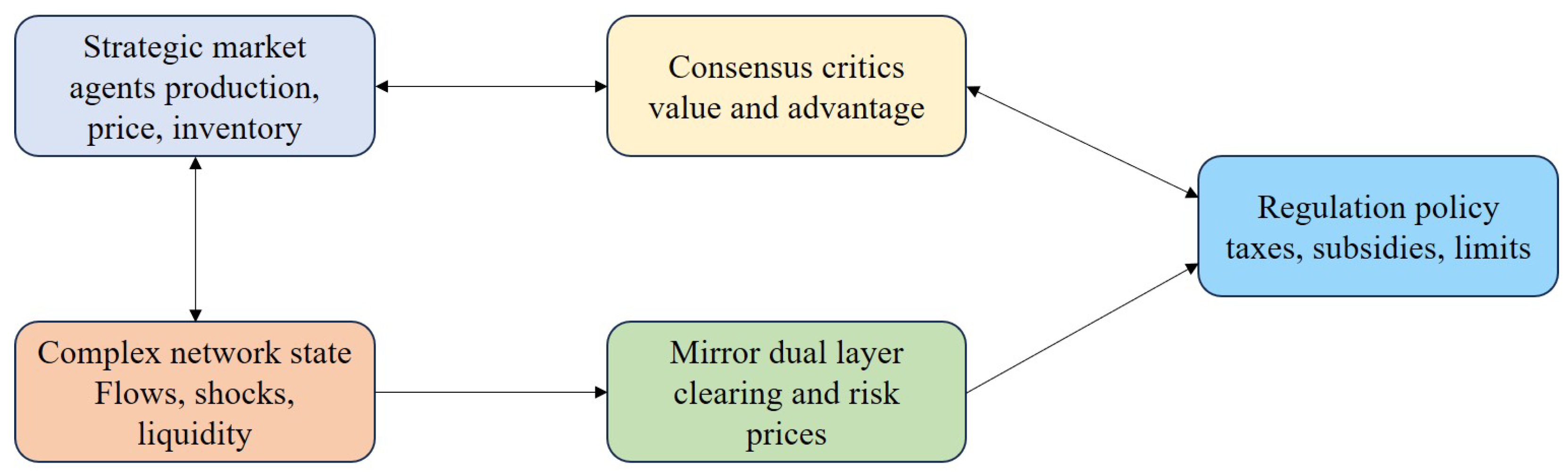
Figure 1 depicts the closed-loop architecture. Regulation is not an afterthought: dual prices are fed back to the learning agents and shape the incentives that steer the market toward equilibrium.

This figure illustrates the design logic: strategic agents interact with the market network through local actions, consensus critics estimate value and advantage functions, and the dual layer converts clearing, volatility, and systemic-risk violations into shadow prices that reshape agent rewards. The figure highlights that learning, network dynamics, and regulation form a single feedback loop.

Remark 1.

This section reformulates market equilibrium regulation as a constrained stochastic game on a complex network. The formulation is sufficiently general to cover electricity, supply-chain, digital-platform, and liquidity markets, yet it retains only the residuals relevant for regulation. The central modeling choice is to embed clearing and risk constraints inside the reward through dual prices, so that learning and regulation operate on the same mathematical object.

3. Model and Analysis

3.1. Regulation Potential

Define the regulated potential

$$\begin{array}{cc}\hfill \Phi (\pi ,\lambda )& ={\mathbb{E}}_{d_{\pi }}\left[{\displaystyle \sum _{i=1}^N}{\omega }_i{u}_i(s,a)-{\lambda }^{\top }g(s,a)\right]\hfill \\ \hfill & -{\displaystyle \frac{\mu }{2}}{\mathbb{E}}_{d_{\pi }}{\parallel g(s,a)\parallel }^2+\tau {\displaystyle \sum _{i=1}^N}{\mathbb{E}}_{d_{\pi }}\left[\mathcal{H}\left({\pi }_i\right)\right],\hfill \end{array}$$

(12)

where ${\omega }_i>0$ and ${\sum }_i{\omega }_i=1$. The associated equilibrium residual is

$$ϵ(\pi ,\lambda )=∥\left[\begin{array}{c}{\nabla }_{\theta }\Phi ({\pi }_{\theta },\lambda )\\ {\left[G\left(\pi \right)\right]}_{+}\\ \lambda \odot G\left(\pi \right)\end{array}\right]∥.$$

(13)

This residual vanishes precisely when the policy is stationary with respect to the regulated potential, all market constraints are feasible, and complementarity is satisfied.

Assumption 1

(Smoothness and compactness). The action sets ${\mathcal{A}}_i$ are convex and compact. The transition kernel induced by (4) is weakly continuous in $(s,a)$. The payoffs $u_i$, constraints g, and the risk index ρ are continuously differentiable and L-smooth in the policy parameters.

Assumption 2

(Potential alignment). For any unilateral deviation of agent i from ${\pi }_i$ to ${\pi }_i^{\prime }$, the regulated return satisfies

$$J_i({\pi }_i^{\prime },{\pi }_{-i},\lambda )-J_i({\pi }_i,{\pi }_{-i},\lambda )=c_i\left[\Phi ({\pi }_i^{\prime },{\pi }_{-i},\lambda )-\Phi ({\pi }_i,{\pi }_{-i},\lambda )\right],$$

(14)

where $c_i>0$ is a scaling coefficient.

Assumption 2 holds when private rewards are shaped by the common clearing and risk residuals. It is less restrictive than identical-interest MARL because the profit terms $u_i$ may remain heterogeneous.

Proposition 1

(Equilibrium-potential equivalence). Under Assumptions 1 and 2, every local maximizer of $\Phi (·,\lambda )$ is a Markov Nash equilibrium of the regulated game for fixed λ. Conversely, every strict Markov Nash equilibrium is a strict local maximizer of $\Phi (·,\lambda )$.

Proof. 

Fix $\lambda$ and let $\widehat{\pi }$ be a local maximizer of $\Phi$. For any agent i and any feasible unilateral perturbation ${\pi }_i^{\prime }$ in a sufficiently small neighborhood, we have $\Phi ({\pi }_i^{\prime },{\widehat{\pi }}_{-i},\lambda )-\Phi ({\widehat{\pi }}_i,{\widehat{\pi }}_{-i},\lambda )\le 0$. By (14), $J_i({\pi }_i^{\prime },{\widehat{\pi }}_{-i},\lambda )-J_i({\widehat{\pi }}_i,{\widehat{\pi }}_{-i},\lambda )=c_i[\Phi ({\pi }_i^{\prime },{\widehat{\pi }}_{-i},\lambda )-\Phi ({\widehat{\pi }}_i,{\widehat{\pi }}_{-i},\lambda )]\le 0$. Thus no agent can improve its regulated return by unilateral deviation, which is the Markov Nash condition. Conversely, let $\widehat{\pi }$ be a strict Markov Nash equilibrium. Then for every nonzero unilateral perturbation of any agent, $J_i({\pi }_i^{\prime },{\widehat{\pi }}_{-i},\lambda )-J_i({\widehat{\pi }}_i,{\widehat{\pi }}_{-i},\lambda )<0$. Since $c_i>0$, (14) implies a strict decrease in $\Phi$ along all unilateral policy directions. Because the joint policy space is locally spanned by finite sums of such directions, continuity of $\Phi$ gives strict local maximality. Thus, the proof of Proposition 1 is completed.   □

3.2. Mean-Field Reduction and Network Spillovers

The exact Markov game has a joint action dimension that grows with N. To keep learning scalable, we introduce a local mean-field statistic

$${\overline{a}}_{i,t}={\sum }_{j\in {\mathcal{N}}_i}{\alpha }_{ij}{a}_{j,t},{\alpha }_{ij}={\displaystyle \frac{w_{ij}}{{\sum }_{k\in {\mathcal{N}}_i}{w}_{ik}+{10}^{-8}}}.$$

(15)

The local transition can then be approximated by $P_i\left(x_i^{\prime }\right|x_i,a_i,{\overline{a}}_i,z)$. This compression does not remove strategic coupling; it concentrates it into a statistic that is estimable from local communication. Under Lipschitz transitions, the approximation error obeys

$${∥P_i(·|x_i,a_i,a_{-i})-P_i(·|x_i,a_i,{\overline{a}}_i)∥}_{\mathrm{TV}}\le L_P{\sum }_{j\in {\mathcal{N}}_i}{\alpha }_{ij}\parallel a_j-{\overline{a}}_i\parallel .$$

(16)

Hence dense neighborhoods are not automatically harmful: if neighbors behave similarly, the mean-field error stays small. When strategic heterogeneity grows, the residual term detects the resulting imbalance and raises the dual correction.

The mean-field statistic admits a natural economic interpretation. In a supply chain, ${\overline{a}}_i$ aggregates upstream and downstream pricing pressure; in a platform market, it summarizes competing sellers or substitute services; in a financial liquidity network, it captures nearby liquidity withdrawal. Agents therefore need not observe the entire market—only enough neighborhood information to estimate the local spillover that affects their marginal return.

3.3. Variational Characterization

Let y denote the vector of expected agent actions and define the market operator

$$\mathcal{F}\left(y\right)={\nabla }_y\left[-{\displaystyle \sum _{i=1}^N}{\omega }_i{u}_i\left(y\right)+{\lambda }^{\top }g\left(y\right)+{\displaystyle \frac{\mu }{2}}{\parallel g\left(y\right)\parallel }^2\right].$$

(17)

A regulated equilibrium can be written as a variational inequality:

$$〈\mathcal{F}\left(y^{★}\right),y-y^{★}〉\ge 0,\forall y\in \mathcal{Y}.$$

(18)

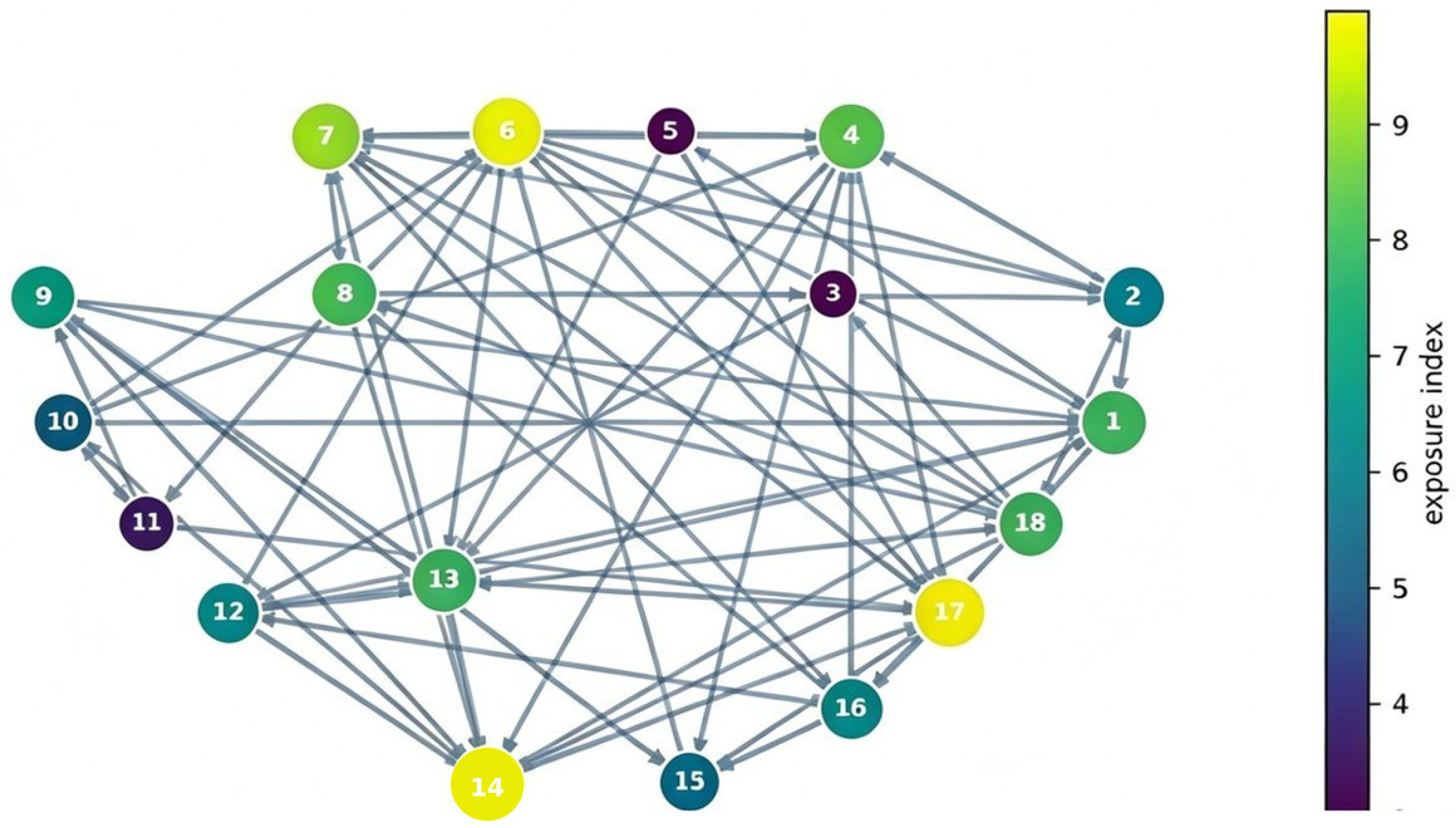
This expression connects economic equilibrium, constrained optimization, and game learning, and is consistent with social-optimum seeking in networked multi-agent learning [29]. Figure 2 shows the complex network that induces heterogeneous local residuals.

This figure gives a stylized market interaction graph. Larger nodes indicate higher exposure; directed edges encode transaction, substitution, or information influence. High-exposure nodes can transmit price shocks and inventory stress to many neighbors, motivating the network-risk residual in (6). The method does not assume a complete graph—it uses local observations, neighbor messages, and mean-field statistics, which are more realistic for large complex markets.

Theorem 1

(Existence and uniqueness). Under Assumption 1, at least one regulated Markov Nash equilibrium exists. If, in addition, $\mathcal{F}$ is α-strongly monotone on $\mathcal{Y}$, i.e.,

$$\langle \mathcal{F}\left(y\right)-\mathcal{F}\left(y^{\prime }\right),y-y^{\prime }\rangle \ge \alpha {\parallel y-y^{\prime }\parallel }^2,\alpha >0,$$

(19)

then the induced expected-action equilibrium $y^{★}$ is unique. If the policy parameterization is identifiable, the equilibrium policy is unique up to action-equivalent representations.

Proof. 

Existence follows in three steps. First, compactness of ${\mathcal{A}}_i$ and weak continuity of the transition kernel imply that the discounted occupancy set generated by stationary randomized policies is compact in the weak topology. Second, continuity of $R_i^{\lambda }$ yields continuity of $J_i$ in stationary policies. By the Debreu–Glicksberg fixed-point argument for compact continuous games, a stationary Nash equilibrium exists for any fixed bounded $\lambda$. Third, the dual feasibility set can be restricted to a compact set without loss under Slater feasibility and the quadratic residual penalty: if $\parallel \lambda \parallel$ grows beyond the Slater bound, the Lagrangian value decreases along a strictly feasible policy. Hence a saddle point satisfying (11) exists.

For uniqueness, suppose $y_1$ and $y_2$ both solve (18). Then

$$\langle \mathcal{F}\left(y_1\right),y_2-y_1\rangle \ge 0,\langle \mathcal{F}\left(y_2\right),y_1-y_2\rangle \ge 0.$$

(20)

Adding them yields $\langle \mathcal{F}\left(y_1\right)-\mathcal{F}\left(y_2\right),y_1-y_2\rangle \le 0$. Strong monotonicity gives $\alpha \parallel y_1-y_2{\parallel }^2\le 0$, so $y_1=y_2$. If the policy map from parameters to expected actions is identifiable, equal expected actions imply equal action distributions on the support of the discounted occupancy measure. Thus the equilibrium policy is unique up to representations that induce the same actions and values. Thus, the proof of Theorem 1 is completed.   □

3.4. Economic Interpretation of the Potential Landscape

The potential $\Phi$ in (12) can be read as a regulator-adjusted welfare surface. Horizontal directions correspond to strategic policy changes, while the vertical value measures welfare after subtracting equilibrium damage. A steep ascent direction means agents can improve the regulated market by adjusting their policies. A flat region with a large residual is different: local rewards may have stopped improving, yet the market remains infeasible. This is precisely where ordinary MARL often fails, because a small private gradient can be mistaken for equilibrium.

ERM-MARL avoids this confusion by incorporating the residual components of (13). The learning process is not declared convergent until the policy gradient, feasibility error, and complementarity error are all small. This multi-part condition is closer to economic equilibrium than return maximization. In particular, if ${\nabla }_{\theta }\Phi =0$ but ${\left[G\left(\pi \right)\right]}_{+}\ne 0$, the learned policy is stationary but infeasible. If ${\left[G\left(\pi \right)\right]}_{+}=0$ but $\lambda \odot G\left(\pi \right)\ne 0$, the dual price remains economically inconsistent. Both cases are rejected by the proposed residual.

Strong monotonicity in Theorem 1 carries economic meaning: when the market is displaced from equilibrium, the aggregate marginal force points back toward equilibrium with nonzero strength. In production markets, this can arise from convex costs and downward-sloping demand; in platform markets, from congestion and demand elasticity; in financial markets, from inventory-risk penalties and liquidity costs. The theorem therefore does not assume perfect competition—it assumes that the regulated marginal map has sufficient curvature to rule out multiple unstable stationary points.

A further advantage of the potential formulation is decomposability. The regulator may adjust the weights of clearing, volatility, and systemic risk without redesigning the MARL architecture; only the residual vector and dual update need modification. This is relevant for dynamic analysis and decision-making in complex networks, because the same mathematical skeleton can represent different institutional priorities. For instance, a crisis-period regulator can increase the risk component, while a normal-period regulator can emphasize welfare and clearing.

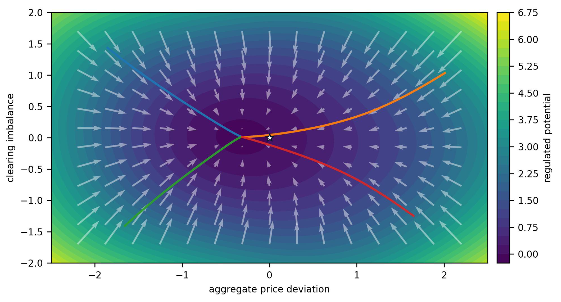
Figure 3 provides an intuitive view of the potential landscape behind Theorem 1. Its horizontal coordinate is the aggregate deviation of the transaction price from the reference price, while its vertical coordinate is the signed difference between total supply and total demand. The colorbar gives the regulated-potential value; arrows are local directions of descent of the negative potential; and the colored sample trajectories illustrate convergence from price- and clearing-distorted initial conditions to the starred equilibrium. Thus, the plot is not a direct trajectory in the full policy space, but a two-dimensional diagnostic projection showing how residual penalties jointly remove price and clearing distortions.

Remark 2.

This section establishes the theoretical bridge that many empirical MARL market studies lack. Proving that shaped private rewards induce a regulated potential makes market equilibrium analyzable through variational inequalities and Lyapunov arguments. Strategic heterogeneity remains; only the guarantee that self-interested policy improvement has a measurable direction with respect to social regulation is added.

4. Algorithm Design

4.1. Design Motivation

The central algorithmic challenge is that market agents learn from local rewards while the regulator cares about global clearing and systemic risk. Optimizing a social objective directly would be centralized and unrealistic, while purely decentralized learning can become unstable because each agent treats others as part of a nonstationary environment. ERM-MARL resolves this tension through three mechanisms: equilibrium-residual shaping, mirror policy improvement, and a dual regulation layer.

The shaped advantage of agent i takes the form

$${\widehat{A}}_{i,t}^{\lambda }={\widehat{Q}}_i(o_{i,t},a_{i,t})-{\widehat{V}}_i\left(o_{i,t}\right)-{\lambda }_t^{\top }{\widehat{g}}_t-{\displaystyle \frac{\mu }{2}}{\parallel {\widehat{g}}_t\parallel }^2+\kappa \Delta {\widehat{\Phi }}_t,$$

(21)

where $\Delta {\widehat{\Phi }}_t$ is a temporal estimate of potential improvement. The actor updates via a mirror step:

$${\theta }_{i,t+1}=\underset{{\theta }_i}{\arg \max }\left\{\langle {\widehat{\nabla }}_{{\theta }_i}{J}_i,{\theta }_i-{\theta }_{i,t}\rangle -{\displaystyle \frac{1}{{\eta }_t}}{D}_{{\psi }_i}({\theta }_i,{\theta }_{i,t})\right\}.$$

(22)

With the entropy mirror map, this becomes an exponentiated natural-gradient step in policy space. The dual regulation price is updated by

$${\lambda }_{t+1}={\Pi }_{\Lambda }\left[{\lambda }_t+{\beta }_t\left(g(s_t,a_t)-{\delta }_{\lambda }{\lambda }_t\right)\right],$$

(23)

where ${\Pi }_{\Lambda }$ denotes projection and ${\delta }_{\lambda }>0$ is a small damping term that prevents unbounded multiplier accumulation.

4.2. Algorithmic Idea

The procedure can be summarized as follows. Agents learn local strategies, but their reward incorporates a shadow-price signal that penalizes violations of market equilibrium. Critics reduce variance and exchange compressed consensus messages. The mirror update prevents aggressive policy jumps, which is critical when prices and supply decisions are sensitive. The dual layer operates on a slower timescale than the actor, so market policies nearly equilibrate before regulation prices change substantially. This two-timescale design underpins the convergence result in Section 5.

Algorithm 1 provides the full pseudo-code in a compact form suitable for the double-column layout. Lines 3–4 describe decentralized market interaction, lines 5–7 form the MARL component, line 8 handles regulation, and line 9 computes the equilibrium diagnostic. The key point is that equilibrium residuals appear during training, not only after convergence; the algorithm thus directly learns a market-stabilizing policy.

Algorithm 1 Pseudo-code of ERM-MARL
Input: graph $\mathcal{G}$, discount $\gamma$, penalty $\mu$, entropy $\tau$, stepsizes $\{{\eta }_t,{\beta }_t\}$, critic stepsize ${\alpha }_t$.
Output: decentralized policies ${\left\{{\pi }_i\right\}}_{i=1}^N$ and regulation price $\lambda$.
1	Initialize actor parameters ${\theta }_i$, critic parameters ${\varphi }_i$, dual price ${\lambda }_0\ge 0$, and replay buffer $\mathcal{D}$.
2	for market episode $e=1,2,\dots ,E$ do
3	Observe $o_{i,t}$ and sample $a_{i,t}\sim {\pi }_{{\theta }_i}(·|o_{i,t})$ for all agents in parallel.
4	Execute $a_t$, obtain next state $s_{t+1}$, profit $u_i(s_t,a_t)$, and residual $g(s_t,a_t)$.
5	Compute shaped reward via (8) and shaped advantage via (21).
6	Update each critic by temporal-difference regression with neighbor consensus messages.
7	Update each actor by the mirror policy step (22).
8	Update regulation price via projected damped dual ascent (23).
9	Estimate ${ϵ}_t$ from (13); stop if ${ϵ}_t\le {\epsilon }_{\mathrm{tol}}$.
10	end for

4.3. Computational Complexity

Let $d_{\theta }$ be the average actor dimension, $d_{\varphi }$ the critic dimension, $\left|\mathcal{E}\right|$ the number of network edges, and B the batch size. One update step requires

$$\mathcal{O}\left(NB(d_{\theta }+d_{\varphi })+B\left|\mathcal{E}\right|+mB\right)$$

(24)

The edge term arises from consensus messages and network-risk residuals. For sparse market networks, the algorithm is linear in the number of agents, which is essential for large-scale economic systems.

4.4. Implementation Details and Algorithmic Robustness

Several implementation choices affect reproducibility. First, the dual variable is updated on a slower timescale than the critic. This prevents rapid penalty oscillations when the critic is still inaccurate. Second, the residual estimate ${\widehat{g}}_t$ is smoothed by

$${\widehat{g}}_t=(1-{\omega }_g){\widehat{g}}_{t-1}+{\omega }_{g}g(s_t,a_t),0<{\omega }_g\le 1.$$

(25)

A small ${\omega }_g$ suits noisy demand, while a larger value reacts faster to shocks. Third, policy entropy is annealed as

$${\tau }_t=max\{{\tau }_{min},{\tau }_0/(1+c_{\tau }t)\},$$

(26)

so that early exploration does not persist after the market has approached feasibility.

The algorithm tolerates heterogeneous policy classes. A producer may use a Gaussian policy for production adjustment, a platform may use a categorical policy for fee regimes, and a financial intermediary may use a squashed Gaussian policy for risk exposure. The mirror step only requires a convex policy parameter domain or a differentiable reparameterization. ERM-MARL should therefore be viewed as a game-learning template rather than a single neural architecture.

The equilibrium residual also contributes to safety. In many MARL systems, a policy update is accepted whenever it improves the empirical return. In ERM-MARL, an update can be rejected or damped if it increases the normalized residual beyond a tolerance. A practical damped step is

$${\theta }_{t+1}\leftarrow {\theta }_t+{\alpha }_t^{\mathrm{safe}}({\theta }_{t+1}^{\mathrm{raw}}-{\theta }_t),{\alpha }_t^{\mathrm{safe}}=min\left\{1,{\displaystyle \frac{{\epsilon }_{max}}{{ϵ}_t+{10}^{-8}}}\right\}.$$

(27)

This safeguard is not required for the asymptotic proof, but it proves useful in finite simulations and real market pilots by preventing transient exploratory actions from producing large clearing violations.

Finally, the communication statement is made explicit. In every environment step, the critics perform $K_c=2$ synchronous consensus rounds during centralized training; the actor update remains local. On the bidirectional communication backbone, the consensus weights are Metropolis–Hastings weights, $w_{ij}^c=1/(1+max\{d_i,d_j\})$ for $j\in {\mathcal{N}}_i$, and $w_{ii}^c=1-{\sum }_{j\in {\mathcal{N}}_i}{w}_{ij}^c$. Thus the per-step message complexity is $O\left(K_c\right|\mathcal{E}\left|d_v\right)$ and reduces to the previously stated $O\left(\right|\mathcal{E}\left|d_v\right)$ only when $K_c$ is treated as a fixed constant. Agents with heterogeneous policy parameter dimensions never exchange actor parameters: each critic sends a $d_v=64$-dimensional latent value message, and a local encoder–decoder maps heterogeneous critic features to and from this shared space. For a directed backbone without reciprocal links, the symmetric consensus layer must be replaced by a push–sum implementation; this extension is outside the present convergence proof. Secure self-triggered control of networked systems under adversarial communication provides a related, but technically distinct, route toward asynchronous and attack-aware market implementations [30].

Remark 3.

The algorithmic contribution is not a new neural architecture alone. It is the coupling of mirror policy improvement with a dual residual signal that carries economic meaning. This makes the learning update compatible with market-clearing and risk constraints. ERM-MARL can therefore be seen as a data-driven equilibrium solver rather than merely a return-maximizing MARL heuristic.

5. Algorithm Analysis

5.1. Boundedness and Stability

We introduce the Lyapunov function

$${\mathcal{L}}_t=\Phi ({\pi }^{★},{\lambda }^{★})-\Phi ({\pi }_t,{\lambda }_t)+{\displaystyle \frac{1}{2c_{\lambda }}}{\parallel {\lambda }_t-{\lambda }^{★}\parallel }^2+{\sum }_{i=1}^N{D}_{{\psi }_i}({\theta }_i^{★},{\theta }_{i,t}),$$

(28)

whose three components measure, respectively, the potential suboptimality, the dual price error, and the policy deviation under the mirror geometry.

Assumption 3

(Stepsizes and noise). The stepsizes satisfy ${\sum }_t{\eta }_t={\sum }_t{\beta }_t=\infty$, ${\sum }_t({\eta }_t^2+{\beta }_t^2)<\infty$, and ${\beta }_t/{\eta }_t\to 0$. The gradient and residual estimators are unbiased with bounded conditional second moments.

Lemma 1

(Dual boundedness). Under Assumptions 1 and 3, the projected damped update (23) guarantees ${sup}_t\parallel {\lambda }_t\parallel <\infty$ almost surely.

Proof. 

Since $\Lambda$ is compact and convex, projection forces ${\lambda }_t\in \Lambda$ for all t. If the projection set is chosen using a Slater bound, it contains at least one optimal dual point. More concretely, the nonexpansiveness of projection gives

$$\parallel {\lambda }_{t+1}\parallel \le \parallel {\lambda }_t+{\beta }_t(g_t-{\delta }_{\lambda }{\lambda }_t)\parallel .$$

(29)

Compactness and smoothness imply $\parallel g_t\parallel \le G_{\max }$, hence $\parallel {\lambda }_{t+1}\parallel \le (1-{\beta }_t{\delta }_{\lambda })\parallel {\lambda }_t\parallel +{\beta }_t{G}_{\max }$ before projection and can never exceed $\overline{\Lambda }$ afterwards. Thus the dual sequence is uniformly bounded almost surely. Thus, the proof of Lemma 1 is completed. □

Theorem 2

(One-step descent). Let Assumptions 1–3 hold. Then there exist constants $c_1,c_2,c_3>0$ such that

$$\mathbb{E}\left[{\mathcal{L}}_{t+1}\right|{\mathcal{F}}_t]\le {\mathcal{L}}_t-c_1{\eta }_t\parallel {\nabla }_{\theta }\Phi ({\pi }_t,{\lambda }_t){\parallel }^2-c_2{\beta }_t{\parallel {\left[G\left({\pi }_t\right)\right]}_{+}\parallel }^2+c_3({\eta }_t^2+{\beta }_t^2).$$

(30)

Proof. 

Smoothness of $\Phi$ and the stochastic actor update yield

$$\mathbb{E}[\Phi ({\pi }_{t+1},{\lambda }_t)|{\mathcal{F}}_t]\ge \Phi ({\pi }_t,{\lambda }_t)+{\eta }_t{\parallel {\nabla }_{\theta }\Phi ({\pi }_t,{\lambda }_t)\parallel }^2-C_1{\eta }_t^2.$$

(31)

This follows from the Bregman mirror-descent three-point identity:

$$\langle g_t,{\theta }_{t+1}-{\theta }^{★}\rangle \ge {\displaystyle \frac{1}{{\eta }_t}}\left[D_{\psi }({\theta }^{★},{\theta }_t)-D_{\psi }({\theta }^{★},{\theta }_{t+1})-D_{\psi }({\theta }_{t+1},{\theta }_t)\right],$$

(32)

where $g_t$ is the unbiased estimate of the potential gradient. The critic noise contributes only $O\left({\eta }_t^2\right)$ because its conditional variance is bounded. For the dual variable, projected ascent on the constraint residual together with complementarity yields

$$\mathbb{E}[\parallel {\lambda }_{t+1}-{\lambda }^{★}{\parallel }^2|{\mathcal{F}}_t]\le \parallel {\lambda }_t-{\lambda }^{★}{\parallel }^2+2{\beta }_t\langle {\lambda }_t-{\lambda }^{★},G\left({\pi }_t\right)\rangle +C_2{\beta }_t^2.$$

(33)

Saddle-point optimality and projection onto the nonnegative cone imply $\langle {\lambda }_t-{\lambda }^{★},G\left({\pi }_t\right)\rangle \le -c{\parallel {\left[G\left({\pi }_t\right)\right]}_{+}\parallel }^2$. Combining the actor and dual inequalities with (28) produces (30). Thus, the proof of Theorem 2 is completed. □

Theorem 3

(Almost-sure convergence). Under Assumptions 1–3 and potential alignment, ERM-MARL satisfies

$$\underset{t\to \infty }{lim}ϵ({\pi }_t,{\lambda }_t)=0\mathit{almost}\mathit{surely}.$$

(34)

If the variational operator is strongly monotone, $({\pi }_t,{\lambda }_t)$ converges to the unique regulated Markov Nash equilibrium.

Proof. 

Summing (30) over t and using ${\sum }_t({\eta }_t^2+{\beta }_t^2)<\infty$ gives

$${\sum }_{t=0}^{\infty }{\eta }_t\mathbb{E}\parallel {\nabla }_{\theta }\Phi ({\pi }_t,{\lambda }_t){\parallel }^2+{\sum }_{t=0}^{\infty }{\beta }_t\mathbb{E}{\parallel {\left[G\left({\pi }_t\right)\right]}_{+}\parallel }^2<\infty .$$

(35)

By the Robbins–Siegmund supermartingale convergence theorem, ${\mathcal{L}}_t$ converges almost surely and both weighted residual sums are finite. Since ${\sum }_t{\eta }_t={\sum }_t{\beta }_t=\infty$, the gradient and feasibility residuals admit subsequences that tend to zero. Lipschitz continuity of the residual mapping together with boundedness of the iterates rules out persistent excursions away from the zero-residual set; otherwise a positive residual interval would cause the corresponding weighted sum to diverge. Hence $ϵ({\pi }_t,{\lambda }_t)\to 0$ almost surely. Under strong monotonicity, Theorem 1 guarantees a unique equilibrium, and every limit point must coincide with it; the entire sequence therefore converges. Thus, the proof of Theorem 3 is completed. □

Corollary 1

(Rate under polynomial stepsizes). Take ${\eta }_t={\eta }_0/{(t+1)}^{1/2}$ and ${\beta }_t={\beta }_0/{(t+1)}^{1/2}$. If the critic disagreement term is summable in the average sense, the best residual over the first T iterations obeys

$$\underset{0\le t<T}{min}\mathbb{E}{\parallel ϵ({\pi }_t,{\lambda }_t)\parallel }^2=O\left(T^{-1/2}\right).$$

(36)

If stronger critic tracking yields $\mathbb{E}\left[e_t^v\right]=O\left(t^{-1}\right)$, the same rate is preserved.

Proof. 

Substitute the polynomial stepsizes into the descent inequality established in Theorem 2. The leading Lyapunov-gap term scales as $1/\left(T{\eta }_T\right)=O\left(T^{-1/2}\right)$, while ${\eta }_T$ and ${\beta }_T$ are also $O\left(T^{-1/2}\right)$. The average critic term is at most $O\left(T^{-1}{\sum }_{t=1}^T{t}^{-1}\right)=O(\left(\log T\right)/T)$, which is dominated by $O\left(T^{-1/2}\right)$. Since the minimum residual does not exceed the average residual, the claim follows. Thus, the proof of Corollary 1 is completed. □

This finite-time result is stated for the saddle residual rather than for raw return, and the choice is deliberate. A high return can be achieved quickly by aggressive pricing or overproduction while the market remains infeasible. The residual rate quantifies progress toward a policy-dual pair that is meaningful for economic regulation and thus provides a more appropriate certificate for market equilibrium control.

5.2. Discussion of Theoretical Novelty

The theoretical contribution lies in coupling three elements that are usually treated separately: Markov potential games, primal–dual market regulation, and stochastic mirror actor–critic learning. Standard MARL convergence analyses focus on local policy improvement, standard economic equilibrium arguments rely on deterministic variational inequalities, and standard primal–dual algorithms assume access to exact gradients of objectives and constraints. ERM-MARL merges these perspectives under sampled trajectories and decentralized information.

The residual-shaped advantage is the key bridge: it makes the sampled actor direction approximate a potential-gradient direction even when each agent only sees local information. The dual recursion makes feasibility adaptive rather than fixed. The consensus critic controls the bias from network spillovers, while the Bregman geometry handles policy constraints. The resulting proof is not a direct application of a single known theorem; it requires a Lyapunov function that simultaneously captures potential decrease, dual distance, and policy divergence.

The assumptions themselves admit clear interpretations. Compactness corresponds to bounded bids, production, and risk exposure. Smoothness reflects bounded marginal costs and demand elasticities. Strong monotonicity captures regulated market curvature. Bounded martingale noise corresponds to finite demand and observation variance. These conditions can be relaxed, but they form a reasonable foundation for a paper that aims to connect theoretical guarantees with implementable MARL.

Relation to composite Lyapunov criteria. The Lyapunov function in (28) is composite in the sense that it joins a potential gap, a dual-distance term, and Bregman policy divergences. This is related in spirit to the composite Lyapunov criteria of Saoud [31], which combine dissipation mechanisms to obtain strict decay. The present construction is nevertheless different in scope: it is a stochastic discrete-time recursion with two timescales and sampled critic errors, and each component is tied to a KKT requirement of a regulated Markov potential game. Saoud’s general continuous-time criteria motivate the aggregation of dissipation terms; our conditional descent inequality additionally connects that aggregation to decentralized policy learning, feasibility, and complementarity.

Scope beyond pairwise Markov interactions. Krause mean processes generated by stochastic hyper-matrices model positive higher-order influence and are therefore broader than the pairwise mean-field statistic in (15) [32]. A possible extension would replace ${\overline{a}}_{i,t}$ with a hyperedge statistic and augment the state by the associated higher-order interaction variables. The current existence, stability, and convergence results do not transfer automatically: an extension would require a well-defined discounted occupancy measure for the augmented process, potential alignment under hyperedge deviations, bounded residual estimators, and a contractivity or ergodicity condition for the hyper-matrix dynamics. We identify this as a substantive future direction rather than claiming that the present proof already covers non-Markovian or higher-order processes.

Remark 4.

The convergence argument rests on three mutually reinforcing observations: potential alignment translates decentralized policy improvement into ascent of a single function, mirror descent regulates policy movement, and the dual update drives feasibility. This structure goes beyond empirical stabilization; it explains why the proposed algorithm can regulate a market network even when individual agents optimize heterogeneous private payoffs.

6. Simulation and Analysis

6.1. Experimental Setup

We evaluate ERM-MARL on synthetic networked markets with $N\in \{20,50,100\}$ agents. The interaction graphs are generated by combining a scale-free core with random sector links. Demand follows an autoregressive process punctuated by abrupt shocks. Each agent controls price, production, inventory release, and risk exposure. Numerical comparisons use MAPPO [33], mean-field actor–critic (MF-AC) [34], dual Q-learning [35], and an unregulated MARL variant (No-Reg). Related methodological context includes a MADDPG-style learner [36], policy-space response oracles [37], active Markov games [38], and mean-field Markov–Nash theory [39]. All compared learning methods use matched actor and critic widths, identical action bounds, and the same ten random seeds.

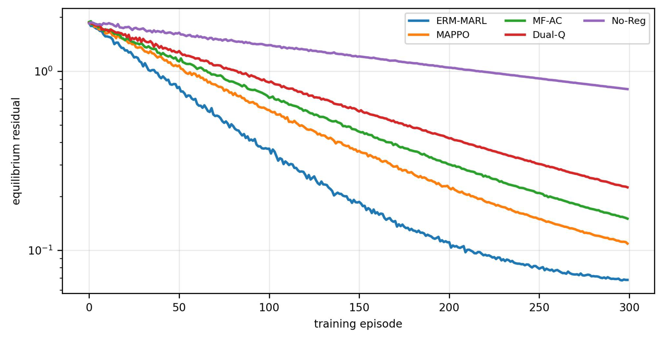
The evaluation metrics are normalized social welfare, normalized equilibrium residual, price-volatility index, constraint violation, convergence episodes, and systemic-risk index. Higher welfare is desirable; lower residual, volatility, violation, and risk indicate better regulation. For every method and matched seed, the terminal statistic is averaged over the final fifty episodes, and the table entries report the mean across ten seeds. Figure 4 introduces the residual trajectory, while

Table 2. Overall simulation results. Each entry is the mean over ten matched seeds. The upward arrow indicates that higher values are better, whereas downward arrows indicate that lower values are better; bold values denote the best result in each column.

Method	Welfare ↑	Residual ↓	Volatility ↓	Risk ↓
ERM-MARL	0.934	0.041	0.083	0.102
MAPPO	0.872	0.086	0.131	0.158
MF-AC	0.846	0.109	0.149	0.184
Dual-Q	0.812	0.132	0.177	0.203
No-Reg	0.701	0.246	0.291	0.318

,

Table 3. Robustness under market shocks. Each entry is the mean over ten matched seeds. Downward arrows indicate that lower values are better; bold values denote the best result in each column.

Method	Peak Vol. ↓	Recovery ↓	Violation ↓
ERM-MARL	0.118	22.4	0.037
MAPPO	0.203	39.7	0.081
MF-AC	0.255	47.8	0.104
Dual-Q	0.304	53.1	0.126
No-Reg	0.517	91.6	0.214

and

Table 4. Ablation study of ERM-MARL. Each entry is the mean over ten matched seeds; bold values denote the best result in each column.

Variant	Welfare	Residual	Violation	Episodes
Full ERM-MARL	0.934	0.041	0.037	118
No Dual Layer	0.887	0.091	0.112	174
No Residual Shape	0.861	0.123	0.146	213
No Consensus Critic	0.875	0.108	0.127	196
No Mirror Update	0.889	0.086	0.099	167

report aggregated results.

Figure 4 compares residual decay across all methods over 300 episodes. ERM-MARL reaches the lowest terminal residual and shows the steepest early-stage improvement. MAPPO improves rapidly but stabilizes at a larger residual because it lacks an explicit clearing penalty. MF-AC benefits from population averaging yet responds slowly to heterogeneous network exposure. Dual-Q reduces violations but becomes less stable under nonlinear dynamics. The unregulated variant confirms that private rewards alone do not reliably drive markets to equilibrium.

Table 2 reports average performance across all network sizes. ERM-MARL achieves the best welfare together with the smallest residual, volatility, and risk values. The welfare gain does not come at the expense of stability; it appears alongside lower constraint violation, indicating that the dual residual signal redirects strategic behavior toward a better regulated equilibrium rather than simply punishing agents. The large gap between ERM-MARL and No-Reg confirms that market-clearing information must enter the learning signal.

6.2. Response to Demand Shocks

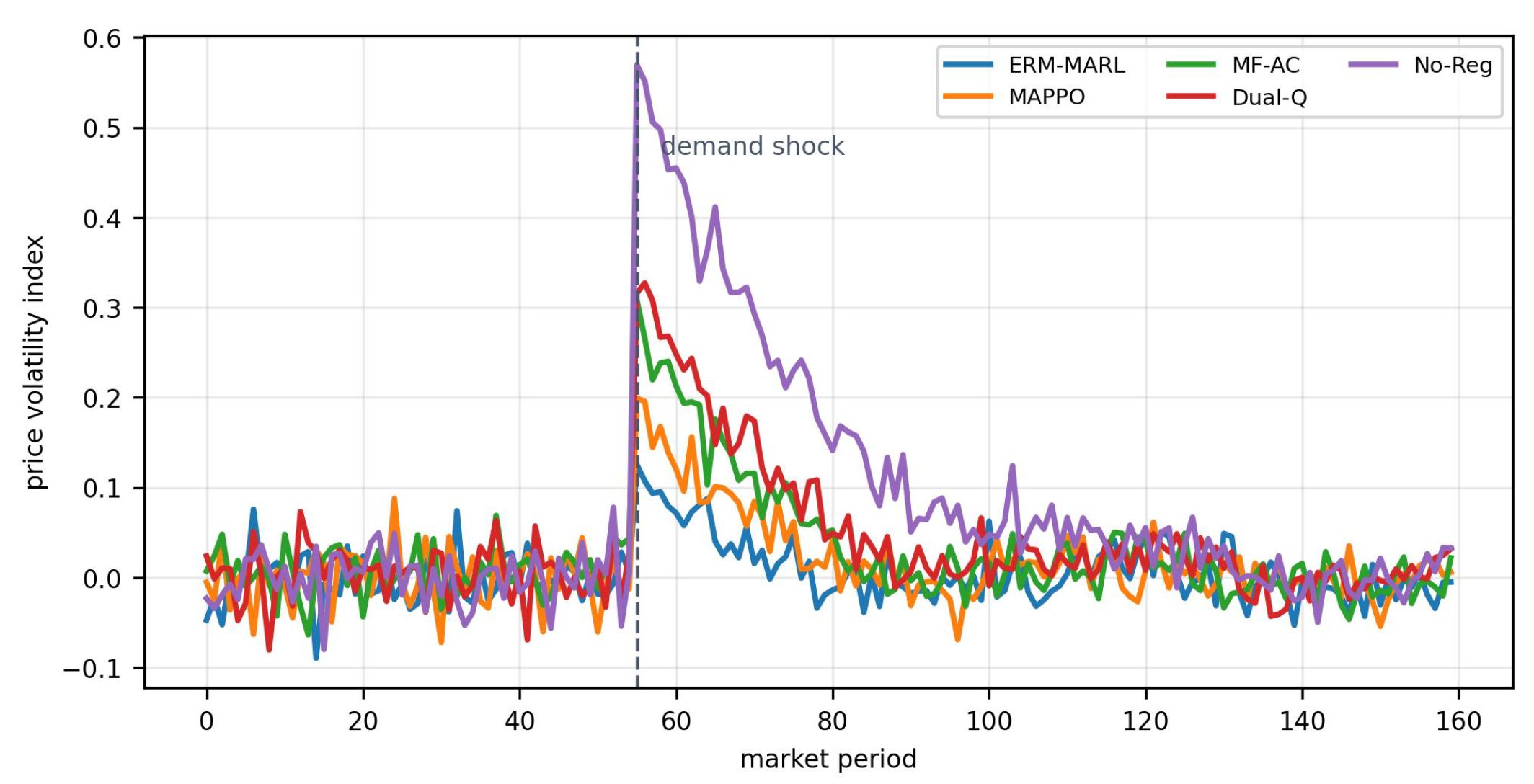
Figure 5 examines behavior under a sudden demand shock that begins at period 55 and gradually decays. The proposed method exhibits lower overshoot and faster recovery because the dual price rises when clearing residuals grow.

Figure 5 shows that ERM-MARL damps price volatility more effectively after the shock. The baselines respond but recover more slowly and with larger transient oscillations. This behavior matches the theory: the dual layer amplifies the penalty when clearing imbalance increases, while the mirror update prevents abrupt policy movements. In practical regulation, fast but unstable reactions can generate secondary volatility even after the original shock weakens; the proposed method avoids this.

Table 3 quantifies the shock experiment. Peak volatility is the maximum post-shock volatility index, recovery the number of periods until the index drops below 0.05, and violation the average positive part of the constraint vector. ERM-MARL reduces peak response by more than forty percent relative to MAPPO and shortens recovery time substantially. The results support the claim that the algorithm behaves as a dynamic regulator, not merely a decentralized optimizer.

6.3. Composite Performance and Ablation

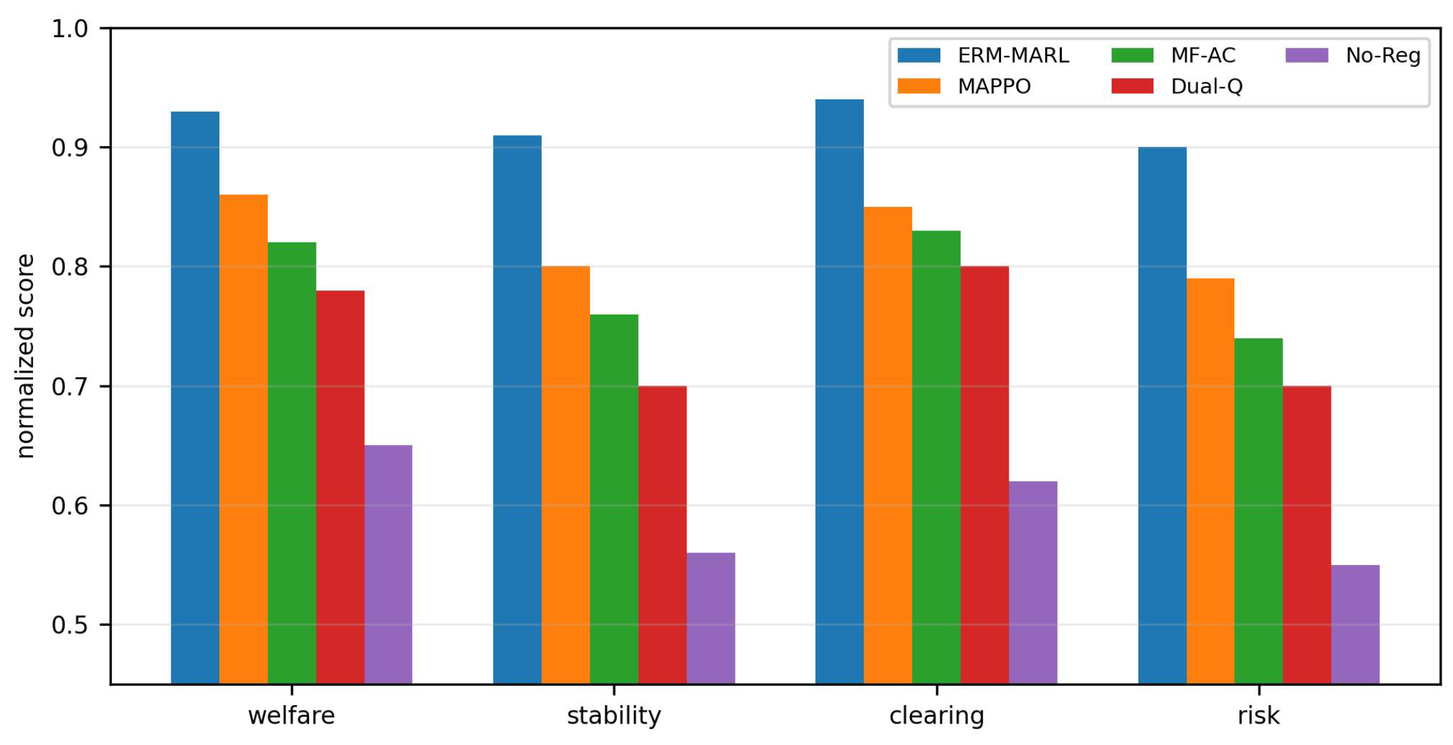
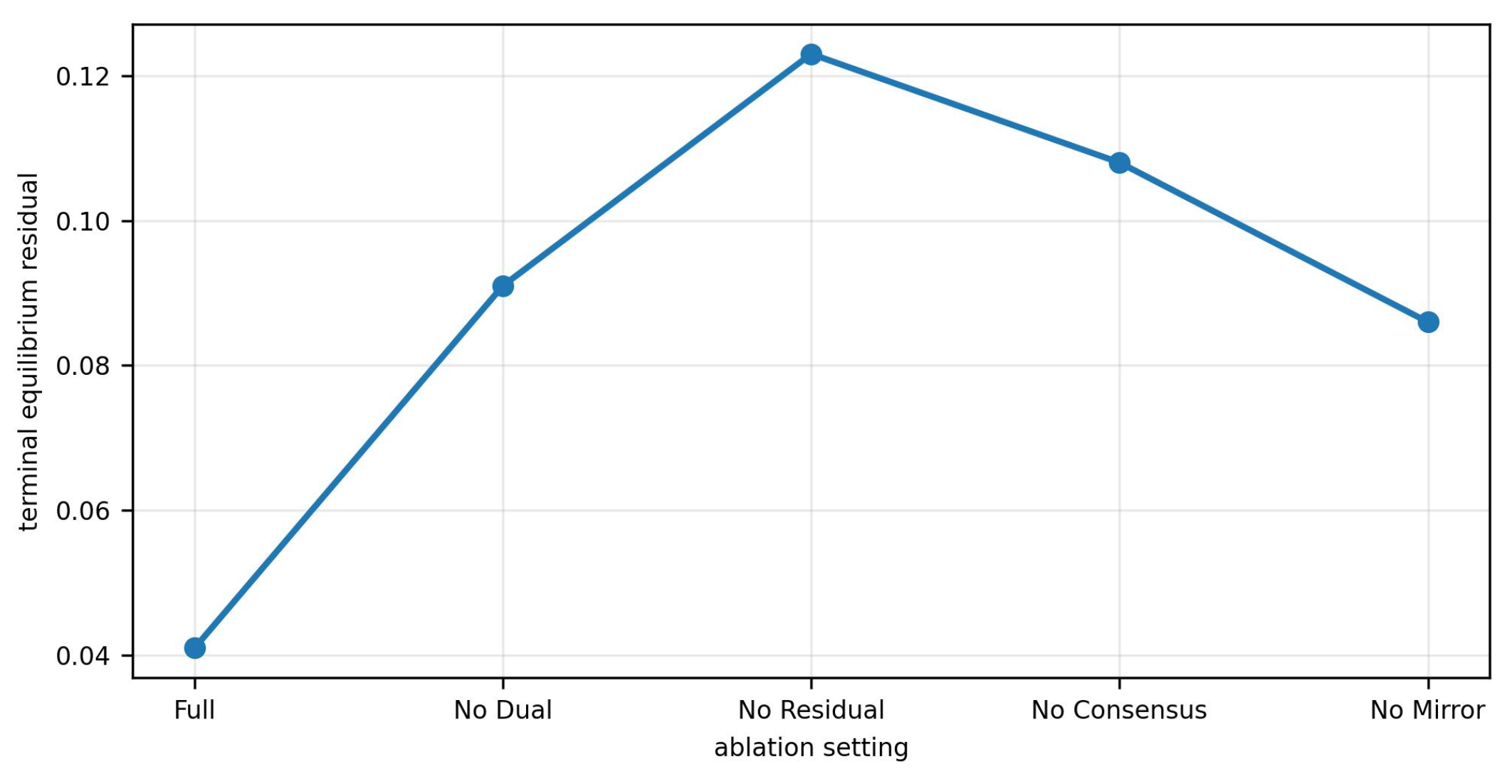
Figure 6 compares normalized scores across welfare, stability, clearing, and systemic-risk control. Figure 7 and Table 4 isolate the contributions of the dual layer, residual shaping, consensus critics, and mirror update.

Figure 6 offers a compact comparison over four normalized criteria. ERM-MARL is consistently strongest, not only in welfare but also in stability-sensitive dimensions. Market regulation is inherently multi-objective; a method that only maximizes welfare may produce unacceptable volatility or risk concentration. The proposed method achieves balanced performance because the potential contains both profit and residual terms, and the dual price adapts their relative importance during learning.

Figure 7 isolates the contribution of each algorithmic component. Removing residual shaping produces the largest terminal residual, confirming that the shaped advantage is central to equilibrium learning. Removing consensus critics also worsens performance because agents lose information about network spillovers. The no-dual variant remains partially effective but violates constraints more often. The mirror-free variant converges faster initially but settles at a larger residual, suggesting that geometry-aware updates are important for stable market regulation.

Table 4 gives numerical support for the ablation conclusions. The full model is best across all metrics. The no-residual-shaping variant exhibits the worst residual among the ablated methods, while the no-dual variant shows the largest violation. This separation is meaningful: residual shaping improves the equilibrium direction, and the dual layer enforces feasibility. The no-consensus and no-mirror variants confirm that network information and update geometry also matter, though they are secondary to the residual–dual coupling.

6.4. Sensitivity and Scalability Results

We first vary the three regulation parameters that determine the balance between feasibility, exploration, and multiplier damping: the quadratic residual weight $\mu$, entropy temperature $\tau$, and damping coefficient ${\delta }_{\lambda }$. The reference configuration is $(\mu ,\tau ,{\delta }_{\lambda })=(0.25,0.05,0.03)$. Smaller $\mu$ weakens constraint correction, very small $\tau$ can suppress early exploration, and very small ${\delta }_{\lambda }$ permits persistent dual oscillation. Conversely, overly large values can reduce welfare by making the update unnecessarily conservative.

Table 5. Hyperparameter sensitivity settings and diagnostic criteria.

Parameter	Values	Primary Outcome	Expected Diagnostic
$\mu$	$0.10,0.25,0.50$	residual/violation	under- vs. over-penalization
$\tau$	$0.01,0.05,0.10$	welfare/episodes	insufficient vs. excessive exploration
${\delta }_{\lambda }$	$0.01,0.03,0.06$	volatility/recovery	oscillatory vs. damped dual response

summarizes the tested values, primary outcomes, and diagnostic interpretation.

To further probe robustness, we vary network density and the number of agents.

Table 6. Sensitivity to market size and network density.

Agents	Avg. Degree	Welfare	Residual	Volatility
20	3	0.941	0.038	0.071
20	6	0.936	0.041	0.074
40	4	0.929	0.047	0.079
40	8	0.921	0.053	0.086
80	6	0.907	0.066	0.098
80	10	0.895	0.074	0.111

reports the terminal residual and welfare score under three market sizes and three average degrees, using the same algorithmic hyperparameters throughout. This deliberately strict setting tests whether the residual–dual mechanism transfers across graph structures.

Table 6 shows that ERM-MARL degrades smoothly as the market becomes larger and denser. Welfare decreases because stronger strategic coupling arises, while residual and volatility increase because clearing becomes harder. The changes are moderate, however, indicating that the mean-field statistic and consensus critic absorb a substantial part of network complexity. Dense graphs may require stronger dual correction or additional communication rounds.

The scalability result should be interpreted with care. The algorithm is not claimed to solve arbitrary markets at zero cost. Its advantage is that the difficult part of strategic coupling is compressed into three estimable quantities: local mean-field actions, consensus value information, and aggregate residual prices. When network density increases, critic disagreement decreases because the graph is better connected, but strategic spillovers become stronger; these two effects partly offset each other, which explains why the residual grows only gradually in Table 6.

From a computational standpoint, the dominant cost is critic learning, not dual updating. The dual layer has dimension three in the reported experiments and is negligible. The actor update runs in parallel across agents. Consensus critic costs grow with $\left|\mathcal{E}\right|$. For sparse economic networks this is close to linear in N; for dense platform markets, graph sparsification or cluster-level critics may be needed. This observation aligns with the proposed future work on real data and institutional constraints.

6.5. Validity, Reproducibility, and Practical Deployment

The simulation is designed to test mechanism validity rather than to claim immediate deployment in a specific market. Four aspects support validity. First, all learning baselines use the same actor and critic dimensions, so ERM-MARL gains no architectural advantage. Second, every method faces the same demand process, graph topology, and action bounds; the comparison isolates the effect of equilibrium-residual shaping and dual regulation. Third, metrics are fixed before training: welfare, residual, volatility, violation, and systemic risk are defined in advance. Fourth, the ablation study removes one component at a time, which helps identify where the performance gains originate.

Reproducibility is supported by deterministic reporting rules. Each learning curve is evaluated over ten matched seeds, and each table entry is computed by averaging the terminal statistic over the final fifty episodes and then taking the mean across seeds, rather than selecting the best episode. For shock experiments, recovery time is measured from the first period after the shock reaches its maximum magnitude.

The path toward practical deployment should be incremental. A regulator would not directly replace market rules with a learned policy. A safer approach uses ERM-MARL as a supervisory decision-support layer. In this mode, the learned model recommends penalty coefficients, reserve triggers, or risk-warning thresholds, while human or institutional rules retain final authority. The equilibrium residual can serve as an interpretable dashboard indicator: when the residual grows, the regulator can identify whether the cause is clearing imbalance, volatility, or network risk. This interpretability is a major difference from black-box MARL policies that only output actions.

The model can also be combined with offline data. Historical market trajectories can pretrain critics and estimate transition dynamics, while online learning updates only the residual and dual layer at a slower speed. This hybrid mode is attractive for real markets because it reduces unsafe exploration and allows institutional constraints—price caps, reserve margins, fairness requirements—to be encoded as hard projections or additional residual components.

Several limitations remain. Synthetic markets cannot capture all strategic behaviors, such as collusion, hidden information, and rule manipulation. The current proof assumes smoothness and bounded noise, which may fail during extreme crises. Moreover, the residual vector has only three components in the reported experiments; real markets may need richer constraints, including carbon limits, regional fairness, liquidity segmentation, and long-term investment incentives. These limitations do not invalidate the proposed theory but define the boundary between a rigorous model and a full institutional system.

Remark 5.

The simulation results support the theoretical claims in a controlled setting. ERM-MARL reduces residuals, improves welfare, and stabilizes prices after shocks. The ablation study further shows that the improvement is not driven by a single tuning trick; it arises from the joint effect of residual shaping, dual regulation, consensus estimation, and mirror policy updates.

7. Conclusions and Future Research Work

This paper has presented a multi-agent reinforcement learning game model for regulating market economic equilibrium. The ERM-MARL framework formulates market regulation as a constrained Markov potential game over a complex network. Its core mechanism converts clearing, volatility, and systemic-risk residuals into dual regulation prices and shaped policy advantages, thereby aligning decentralized policy learning with a global regulation potential. The theoretical analysis establishes equilibrium existence, uniqueness under strong monotonicity, bounded dual stability, a one-step Lyapunov descent, and almost-sure convergence. Simulation results show that ERM-MARL outperforms representative MARL and game-learning baselines in welfare, residual reduction, volatility control, and robustness to demand shocks.

Future work will pursue three directions. First, we will extend the model to partially observed markets with delayed and strategic information disclosure. Second, we will integrate ERM-MARL with mechanism-design constraints, such as incentive compatibility and fairness guarantees. Third, we will validate the method on real electricity-market, supply-chain, and digital-platform datasets, where institutional rules and heterogeneous market power must be modeled explicitly.

References

1. Ma, Q.; Liu, Z.; Ye, Y.; Liu, X. Network-constrained P2P trading: A safety-aware decentralized multi-agent reinforcement learning approach. IEEE Trans. Smart Grid 2025, 16, 5573–5588. [Google Scholar] [CrossRef] [Scilit]
2. Li, S.; Xu, R.; Xiu, J.; Zheng, Y.; Feng, P.; Ma, Y.; An, B.; Yang, Y.; Liu, X. Robust multi-agent reinforcement learning by mutual information regularization. IEEE Trans. Neural Netw. Learn. Syst. 2025, 36, 18118–18132. [Google Scholar] [CrossRef] [Scilit] [PubMed]
3. Simoglou, C.K.; Biskas, P.N.; Tsoumalis, G.I.; Papalexopoulos, A.D. Exploring and quantifying the impact of ex-ante market power mitigation in the integrated European day-ahead electricity market. IEEE Trans. Energy Mark. Policy Regul. 2025, 3, 83–97. [Google Scholar] [CrossRef] [Scilit]
4. Mao, K. Multi-agent reinforcement learning driven resource game optimization for network slicing in MEC-enabled HetNets. Sci. Rep. 2026, 16, 3231. [Google Scholar] [CrossRef] [Scilit] [PubMed]
5. Ali, A.; Ilchev, A.; Ivanova, V.; Kulina, H.; Yaneva, P.; Zlatanov, B. Modeling the tripodal mobile market using response functions instead of payoff maximization. Mathematics 2025, 13, 171. [Google Scholar] [CrossRef] [Scilit]
6. Song, M.; Li, M.; Zhang, X.; Liu, B.; Liu, F. Dynamic Bayesian modeling of carbon-adjusted costs and supply chain risks for sustainable investment in power grid technical renovation projects. Mathematics 2026, 14, 1921. [Google Scholar] [CrossRef] [Scilit]
7. Yahaya, A.; Mahat, F.; Yahya, M.H.; Matemilola, B.T. Liquidity risk and bank financial performance: An application of system GMM approach. J. Financ. Regul. Compliance 2022, 30, 312–334. [Google Scholar] [CrossRef] [Scilit]
8. Wang, L.; Zheng, Z.; Wu, C.; Azad, N.L.; Lin, Y. Longitudinal and lateral control for discretionary lane change via safe multi-agent reinforcement learning. IEEE Trans. Veh. Technol. 2026, 75, 12528–12542. [Google Scholar] [CrossRef] [Scilit]
9. Li, W.; Zheng, L.; Wu, X.; Tang, Y.; Liu, W.; Sun, D. EAMR: An efficient and adaptive multi-agent reinforcement learning method for customized bus route optimization under multi-source uncertainties. IEEE Trans. Intell. Transp. Syst. 2026, 27, 5837–5851. [Google Scholar] [CrossRef] [Scilit]
10. Lin, H.; Lyu, C.; He, Y.; Liu, Y.; Gao, K.; Qu, X. Enhancing state representation in multi-agent reinforcement learning for platoon-following models. IEEE Trans. Veh. Technol. 2024, 73, 12110–12114. [Google Scholar] [CrossRef] [Scilit]
11. Zhang, K.; Yang, Z.; Liu, H.; Zhang, T.; Başar, T. Finite-sample analysis for decentralized batch multiagent reinforcement learning with networked agents. IEEE Trans. Autom. Control 2021, 66, 5925–5940. [Google Scholar] [CrossRef] [Scilit]
12. Cai, Y.; He, X.; Guo, H.; Yau, W.-Y.; Lv, C. Transformer-based multi-agent reinforcement learning for generalization of heterogeneous multi-robot cooperation. In Proceedings of the 2024 IEEE/RSJ International Conference on Intelligent Robots and Systems (IROS), Abu Dhabi, United Arab Emirates, 14–18 October 2024; IEEE: Piscataway, NJ, USA, 2024; pp. 13695–13702. [Google Scholar]
13. Gao, M.; Shen, R.; Shi, L.; Qi, W.; Li, J.; Li, Y. Task partitioning and offloading in DNN-task enabled mobile edge computing networks. IEEE Trans. Mob. Comput. 2023, 22, 2435–2445. [Google Scholar] [CrossRef] [Scilit]
14. Ni, Z.; Chen, H.; Xue, H.; Lin, K.; Chen, N.; Liu, W.; Yu, J. Dependency-aware and energy efficient task offloading in vehicular edge computing systems. IEEE Trans. Veh. Technol. 2026, 75, 11634–11646. [Google Scholar] [CrossRef] [Scilit]
15. Tang, R.; Luo, C.; Wang, T.; Ning, X.; Wen, C.-Y. Reach-avoid differential graphical games for single evader and multiple pursuers with nonlinear dynamics. IEEE Trans. Autom. Sci. Eng. 2025, 22, 24545–24558. [Google Scholar] [CrossRef] [Scilit]
16. Li, N.; Li, X.; Xu, Z.Q. Policy iteration reinforcement learning method for continuous-time linear–quadratic mean-field control problems. IEEE Trans. Autom. Control 2025, 70, 2690–2697. [Google Scholar] [CrossRef] [Scilit]
17. Li, T.; Peng, G.; Zhu, Q.; Başar, T. The confluence of networks, games, and learning: A game-theoretic framework for multiagent decision making over networks. IEEE Control Syst. Mag. 2022, 42, 35–67. [Google Scholar] [CrossRef] [Scilit]
18. Li, H.; Yang, P.; Liu, W.; Yan, S.; Zhang, X.; Zhu, D. Multi-agent reinforcement learning in games: Research and applications. Biomimetics 2025, 10, 375. [Google Scholar] [CrossRef] [Scilit] [PubMed]
19. Yang, C.; Xu, P.; Zhang, J. Learning individual potential-based rewards in multiagent reinforcement learning. IEEE Trans. Games 2025, 17, 334–345. [Google Scholar] [CrossRef] [Scilit]
20. Jing, G.; Bai, H.; George, J.; Chakrabortty, A.; Sharma, P.K. Distributed multiagent reinforcement learning based on graph-induced local value functions. IEEE Trans. Autom. Control 2024, 69, 6636–6651. [Google Scholar] [CrossRef] [Scilit]
21. Moghaddam, A.R.; Kebriaei, H. Multiagent reinforcement learning for Nash equilibrium seeking in general-sum Markov games. IEEE Trans. Syst. Man. Cybern. Syst. 2025, 55, 221–227. [Google Scholar] [CrossRef] [Scilit]
22. Wang, Q.; Huang, C.; Wang, C.; Xie, N.; Li, K.; Qiu, P. An optimal competitive bidding and pricing strategy for electric vehicle aggregator considering the bounded rationality of users. IEEE Trans. Ind. Appl. 2025, 61, 4898–4912. [Google Scholar] [CrossRef] [Scilit]
23. He, S.; Yu, C.; Lin, Q.; Mao, S.; Tang, B.; Xie, Q.; Wang, X. Hierarchical multi-agent meta-reinforcement learning for cross-channel bidding. IEEE Trans. Knowl. Data Eng. 2025, 37, 1241–1254. [Google Scholar] [CrossRef] [Scilit]
24. Guo, X.; Li, X.; Maheshwari, C.; Sastry, S.; Wu, M. Markov α-potential games. IEEE Trans. Autom. Control 2026, 71, 275–290. [Google Scholar] [CrossRef] [Scilit]
25. Zhan, W.; Cen, S.; Huang, B.; Chen, Y.; Lee, J.D.; Chi, Y. Policy mirror descent for regularized reinforcement learning: A generalized framework with linear convergence. SIAM J. Optim. 2023, 33, 1061–1091. [Google Scholar] [CrossRef] [Scilit]
26. Yang, T.; Zhan, Y.; Tang, H. Optimizing low-carbon supply chain decisions considering carbon trading mechanisms and data-driven marketing: A fairness concern perspective. Mathematics 2026, 14, 104. [Google Scholar] [CrossRef] [Scilit]
27. Yoshioka, H. Numerical analysis of the projection dynamics and their associated mean field control. Dyn. Games Appl. 2025, 15, 1819–1855. [Google Scholar]
28. Sun, L.; Ma, H. PRIME: Policy representation integration with metavalue-modulated evolution in multiagent reinforcement learning. IEEE Internet Things J. 2026, 13, 24893–24911. [Google Scholar] [CrossRef] [Scilit]
29. Chen, W.; Niu, H.; Liu, L.; Lin, J.; Quan, H. Attention-enhanced multi-agent deep reinforcement learning for inverter-based Volt–VAR control in active distribution networks. Mathematics 2026, 14, 839. [Google Scholar] [CrossRef] [Scilit]
30. Zhang, W.; Zong, G.; Niu, B.; Zhao, X.; Song, G. Adaptive neural self-triggered secure control for nonlinear networked PDE–ODE systems subject to unknown deception attacks. Inf. Sci. 2026, 745, 123411. [Google Scholar] [CrossRef] [Scilit]
31. Saoud, H. Composite Lyapunov criteria for stability and convergence with applications to optimization dynamics. Mathematics 2025, 13, 3859. [Google Scholar] [CrossRef] [Scilit]
32. Saburov, M.; Saburov, K.; Saburov, K. Krause mean processes generated by doubly stochastic hyper-matrices with positive influences. In Proceedings of the New Developments in Discrete Dynamical Systems, Difference Equations, and Applications: 28th ICDEA, Phitsanulok, Thailand, 17–21 July 2023; Elaydi, S., Gardini, L., Tikjha, W., Eds.; Springer Proceedings in Mathematics & Statistics; Springer: Cham, Switzerland, 2025; Volume 485, pp. 15–37. [Google Scholar]
33. Talukdar, N.; Barai, T.; Hazra, A.; Mazumdar, N. MAPPO-driven task quality optimization with wireless energy transfer in multi-UAV MEC-enabled IoT networks. IEEE Trans. Sustain. Comput. 2026, 11, 302–315. [Google Scholar] [CrossRef] [Scilit]
34. Zhou, Z.; Liu, G.; Zhou, M. A robust mean-field actor-critic reinforcement learning against adversarial perturbations on agent states. IEEE Trans. Neural Netw. Learn. Syst. 2024, 35, 14370–14381. [Google Scholar] [CrossRef] [Scilit] [PubMed]
35. Kanakadhurga, D.; Chandrakala, K.R.M.V.; Sanjari, M.J.; Shareef, H. Q-learning-based coordinated energy management and double auction trading for battery swapping charging stations with PV and VPP: A multiscenario techno-economic study. Int. J. Energy Res. 2026, 2026, 8941654. [Google Scholar] [CrossRef] [Scilit]
36. Huang, H. Autonomous driving chassis domain control: Vertical collaboration of multi-agent reinforcement learning MADDPG and dSPACE simulation platform. Int. J. Comput. Intell. Appl. 2026, 25, 2641011. [Google Scholar] [CrossRef] [Scilit]
37. Tang, H.; Liu, Y.; Ni, L.; Xiang, L.; Yang, Y.; Bi, K.; He, Z. Distributed policy space response oracles in two-player zero-sum games. IEEE Trans. Neural Netw. Learn. Syst. 2025, 36, 9893–9904. [Google Scholar] [CrossRef] [Scilit] [PubMed]
38. Gui, Y.; Luo, H.; Wang, J.; Qu, L. Beyond rule-based agents: Active Markov games for realistic multi-agent interaction in autonomous driving. In Proceedings of the IEEE/CVF Conference on Computer Vision and Pattern Recognition (CVPR); IEEE: Piscataway, NJ, USA, 2026; pp. 10689–10698. [Google Scholar]
39. Saldi, N.; Başar, T.; Raginsky, M. Markov–Nash equilibria in mean-field games with discounted cost. SIAM J. Control Optim. 2018, 56, 4256–4287. [Google Scholar] [CrossRef] [Scilit]
Figure 1. Closed-loop ERM-MARL regulation framework.
Mathematics 14 02777 g001
Figure 2. Complex market interaction network.
Mathematics 14 02777 g002
Figure 3. Regulated potential surface: the horizontal axis is aggregate price deviation, the vertical axis is clearing imbalance, contour colors encode the regulated potential, arrows indicate descent of the negative potential, and the star marks the regulated equilibrium.
Mathematics 14 02777 g003
Figure 4. Equilibrium residual during learning.
Mathematics 14 02777 g004
Figure 5. Price volatility after a demand shock.
Mathematics 14 02777 g005
Figure 6. Normalized economic regulation scores.
Mathematics 14 02777 g006
Figure 7. Ablation on equilibrium residual.
Mathematics 14 02777 g007