A Caputo Fractional SLBS Computer Virus Model with Stage-Specific Holling Type-II Incidence

Abstract

Computer virus propagation (CVP) models translate malware movement in a network into analyzable dynamical systems. Two features are especially important for modern networks: infected hosts may remain latent before a damaging burst, and infection efficiency is usually saturated by limited contacts, filtering, isolation, or response resources. This article develops a two-dimensional Caputo fractional susceptible–latent–bursting–susceptible (SLBS) CVP model in which the susceptible–latent and susceptible–bursting channels have different Holling type-II incidence functions. The fractional derivative represents memory effects in the propagation process, while the two incidence functions allow the latent and bursting stages to have separate transmission strengths and saturation levels. Non-negativity, boundedness, and well-posedness are established. The system is then used to derive the basic reproduction number, classify all endemic equilibria, and obtain local asymptotic stability criteria for the virus-free, latency-free burst-endemic, and latency–burst coexistence equilibria. Numerical simulations based on an Adams predictor–corrector scheme illustrate the theoretical thresholds and suggest global convergence in representative parameter regions. The results provide a stage-sensitive modeling tool for analyzing and designing targeted defense policies against computer virus outbreaks.

1. Introduction

Malware spreading in a computer network is often studied with ideas borrowed from epidemic theory [1]. A node that receives malicious code can transmit it to other nodes, and the aggregate behavior can be represented by compartmental dynamical systems [2,3]. Such CVP models are useful because they turn qualitative security questions—for example, whether a patching policy can stop an outbreak—into threshold and stability questions that can be analyzed mathematically. Early models and many of their later extensions usually start from bilinear infection terms [4,5,6,7]; a review of this modeling direction is given in [8].

Bilinear incidence is convenient, but it is rarely a complete description of a real network. When the number of compromised hosts increases, bandwidth, scanning opportunities, firewall rules, intrusion detection, quarantine decisions, and user responses may all limit additional infections. This motivates saturated or otherwise nonlinear incidence terms. Nonlinear infection functions have therefore been introduced into several CVP frameworks to represent contact limitation and defensive feedback more realistically [9,10,11,12].

Another feature of many malicious programs is a delay between infection and visible damage. A compromised host can stay in a latent state while it scans, waits for a trigger, or keeps communication covert; after activation, the same host may enter a bursting state and perform destructive operations. This behavior has led to susceptible–latent–bursting–susceptible (SLBS) models [13,14,15,16,17,18,19] and related variants [20,21,22]. In practical networks, the latent and bursting stages need not infect through the same mechanism. Latent infection may be limited by stealthy scanning or covert messaging, whereas bursting infection may be limited by visible damage, emergency isolation, or rapid repair. Treating both stages as a single infection pool may therefore hide stage-specific security effects.

Fractional-order derivatives add another layer to CVP modeling [23]. They allow the rate of change to depend on earlier states, which is appropriate when infection, detection, and repair are influenced by accumulated network history. Fractional CVP models have been considered in several recent studies [24,25,26,27,28]. Recently, Liu et al. [29] proposed a Caputo fractional SLBS model with a Holling type-II saturation effect. To our knowledge, this is the only known fractional SLBS model. In that model, the susceptible–latent and susceptible–bursting infection components are

$${\displaystyle \frac{\beta S\left(t\right)L\left(t\right)}{1+\sigma \left[L\right(t)+B(t\left)\right]}}$$

and

$${\displaystyle \frac{\beta S\left(t\right)B\left(t\right)}{1+\sigma \left[L\right(t)+B(t\left)\right]}},$$

respectively. Equivalently, the susceptible equation contains the unified susceptible–(latent + bursting) saturated infection term

$$\beta {\displaystyle \frac{S\left(t\right)\left[L\right(t)+B(t\left)\right]}{1+\sigma \left[L\right(t)+B(t\left)\right]}}.$$

This formulation is meaningful when latent and bursting nodes share the same infection force and jointly contribute to one common saturation pool. Nevertheless, it is restrictive in scenarios where the two infected states have different propagation capabilities or are limited by different saturation mechanisms.

Motivated by this observation, the present article proposes a new Caputo fractional SLBS model with a pair of Holling type-II saturation infection rates. Specifically, the susceptible–latent infection rate is modeled as

$${\displaystyle \frac{{\beta }_{1}S\left(t\right)L\left(t\right)}{1+{\theta }_{1}L\left(t\right)}},$$

while the susceptible–bursting infection rate is modeled as

$${\displaystyle \frac{{\beta }_{2}S\left(t\right)B\left(t\right)}{1+{\theta }_{2}B\left(t\right)}}.$$

Here, ${\beta }_1$ and ${\theta }_1$ describe the infection force and saturation intensity of the latent-infection channel, whereas ${\beta }_2$ and ${\theta }_2$ describe those of the bursting-infection channel. This model is not merely a reparameterization of [29]; rather, it represents a channel-specific saturation mechanism. Even if ${\beta }_1={\beta }_2$ and ${\theta }_1={\theta }_2$, the proposed infection structure does not reduce to the unified denominator $1+\sigma \left[L\right(t)+B(t\left)\right]$ used in [29]. Hence, the proposed model provides a different and stage-sensitive description of virus spread.

Table 1. Differences between the model assumptions of the two models.

Aspect	The Previous Model	Our Model
Infection structure	Unified saturated infection mechanism for susceptible–(latent + bursting) transmission	Two channel-specific Holling type-II infection mechanisms
Susceptible–latent infection term	${\displaystyle \frac{\beta SL}{1+\sigma (L+B)}}$	${\displaystyle \frac{{\beta }_{1}SL}{1+{\theta }_{1}L}}$
Susceptible–bursting infection term	${\displaystyle \frac{\beta SB}{1+\sigma (L+B)}}$	${\displaystyle \frac{{\beta }_{2}SB}{1+{\theta }_{2}B}}$
Infection forces	A common infection force $\beta$ is used for both latent and bursting nodes	Different infection forces ${\beta }_1$ and ${\beta }_2$ are allowed
Saturation mechanism	A common saturation denominator $1+\sigma (L+B)$ is used	Separate saturation denominators $1+{\theta }_{1}L$ and $1+{\theta }_{2}B$ are used
Modeling implication	Latent and bursting nodes jointly contribute to one saturation pool	Latent-driven and bursting-driven infections can saturate differently

highlights the differences between the model assumptions of the model published in [29] and our model, whereas

Table 2. Differences between the mathematical results of the two models.

Aspect	The Previous Model	Our Model
Threshold structure	$R_0$ is governed by one infection force $\beta$ and the residence/removal structure of the two infected stages	$R_0=max(R_1,R_2)$ with $R_1={\displaystyle \frac{{\beta }_1\mu }{\delta (\eta +\delta )}}$ and $R_2={\displaystyle \frac{{\beta }_2\mu }{\delta (\gamma +\delta )}}$, so the dominant channel depends on channel-specific infection forces and stage-specific transmission/removal rates
Latency-endemic burst-free equilibria	There is no latency-endemic burst-free equilibrium	There is no latency-endemic burst-free equilibrium
Latency-free burst-endemic equilibria	There is no latency-free burst-endemic equilibrium if $R_2\le 1$. There is the sole latency-free burst-endemic equilibrium $E_1=\left(0,{\displaystyle \frac{(\gamma +\delta )(R_2-1)}{\beta +(\gamma +\delta )\sigma }}\right)$ if $R_2>1$	There is no latency-free burst-endemic equilibrium if $R_2\le 1$. There is the sole latency-free burst-endemic equilibrium $E_1=\left(0,{\displaystyle \frac{(\gamma +\delta )(R_2-1)}{{\beta }_2+(\gamma +\delta ){\theta }_2}}\right)$ if $R_2>1$
Latency-endemic burst-endemic equilibria	There is no latency-endemic burst-endemic equilibrium if $R_1\le 1$ or $\gamma \le \eta$. There is the sole latency-endemic burst-endemic equilibrium $E_2=\left({\displaystyle \frac{(\gamma -\eta )(\eta +\delta )(R_1-1)}{\gamma [\beta +(\eta +\delta \left)\sigma \right]}},{\displaystyle \frac{\eta (\eta +\delta )(R_1-1)}{\gamma [\beta +(\eta +\delta \left)\sigma \right]}}\right)$ if $R_1>1$ and $\gamma >\eta$	There is no latency-endemic burst-endemic equilibrium if $R_1\le 1$ or $r^{*}\ge {\displaystyle \frac{(\eta +\delta )(R_1-1)}{{\beta }_1}}$. There is the sole latency-endemic burst-endemic equilibrium $E_2=\left({\displaystyle \frac{(\eta +\delta )(R_1-1)-{\beta }_1{r}^{*}}{{\beta }_1+(\eta +\delta ){\theta }_1}},r^{*}\right)$ if $R_1>1$ and $r^{*}<{\displaystyle \frac{(\eta +\delta )(R_1-1)}{{\beta }_1}}$
Local stability of the virus-free equilibrium $E_0$	$E_0$ is asymptotically stable or unstable according to $R_0<1$ or $R_0>1$	$E_0$ is asymptotically stable or unstable according to $R_0<1$ or $R_0>1$
Local stability of $E_1$	$E_1$ is asymptotically stable if $|arg\left({\lambda }_1\right)| >{\displaystyle \frac{\alpha \pi }{2}}$ and $|arg\left({\lambda }_2\right)| >{\displaystyle \frac{\alpha \pi }{2}}$. $E_1$ is unstable if $|arg\left({\lambda }_1\right)| <{\displaystyle \frac{\alpha \pi }{2}}$ or $|arg\left({\lambda }_2\right)| <{\displaystyle \frac{\alpha \pi }{2}}$	$E_1$ is asymptotically stable if $|arg\left({\lambda }_1\right)| >{\displaystyle \frac{\alpha \pi }{2}}$ and $|arg\left({\lambda }_2\right)| >{\displaystyle \frac{\alpha \pi }{2}}$. $E_1$ is unstable if $|arg\left({\lambda }_1\right)| <{\displaystyle \frac{\alpha \pi }{2}}$ or $|arg\left({\lambda }_2\right)| <{\displaystyle \frac{\alpha \pi }{2}}$
Local stability of $E_2$	$E_2$ is asymptotically stable if $|arg\left({\lambda }_1\right)| >{\displaystyle \frac{\alpha \pi }{2}}$ and $|arg\left({\lambda }_2\right)| >{\displaystyle \frac{\alpha \pi }{2}}$. $E_2$ is unstable if $|arg\left({\lambda }_1\right)| <{\displaystyle \frac{\alpha \pi }{2}}$ or $|arg\left({\lambda }_2\right)| <{\displaystyle \frac{\alpha \pi }{2}}$	$E_2$ is asymptotically stable if $|arg\left({\lambda }_1\right)| >{\displaystyle \frac{\alpha \pi }{2}}$ and $|arg\left({\lambda }_2\right)| >{\displaystyle \frac{\alpha \pi }{2}}$. $E_2$ is unstable if $|arg\left({\lambda }_1\right)| <{\displaystyle \frac{\alpha \pi }{2}}$ or $|arg\left({\lambda }_2\right)| <{\displaystyle \frac{\alpha \pi }{2}}$

stresses the differences between the mathematical results of the two models.

The remainder of this article is organized as follows: Section 2 outlines the fundamental knowledge underpinning this research. Section 3 formulates the new fractional SLBS model. Section 4 and Section 5 analyze the basic properties of this model. Section 6 identifies all virus-endemic equilibria of the model. Section 7 examines the local stability of all equilibria. Section 8 inspects the global stability of these equilibria through numerical experiments. Section 9 makes further discussions. Section 10 closes this work.

2. Preliminaries

This section records several standard facts from fractional calculus and linear fractional systems that will be used later.

Definition 1

([23]). For a complex argument z with positive real part, the Gamma function is

$$\mathsf{\Gamma }\left(z\right)={\int }_0^{+\infty }{t}^{z-1}{e}^{-t}dt.$$

(1)

This function is one of the most fundamental special functions in mathematics. It extends the factorial operation from positive integers to real and complex numbers.

Definition 2

([23]). For a complex number α with positive real part and a complex number z, the one-parameter Mittag–Leffler function is

$$E_{\alpha }\left(z\right)={\displaystyle \sum _{k=0}^{+\infty }}{\displaystyle \frac{z^k}{\mathsf{\Gamma }(\alpha k+1)}}.$$

(2)

This function is a cornerstone special function in modern mathematics and applied sciences. As a natural generalization of the exponential function, it serves as the fundamental solution to linear fractional differential systems, which describe systems with long-term memory, non-locality, and power-law delay.

Definition 3.

Let $0<\alpha <1$, $f:[0,\infty )\to \mathbb{R}$ be a differential function. The α-order Caputo derivative of f is defined to be

$$D^{\alpha }f\left(t\right)={\displaystyle \frac{1}{\mathsf{\Gamma }(1-\alpha )}}{\int }_0^t{\displaystyle \frac{f^{\prime }\left(s\right)}{{(t-s)}^{\alpha }}}ds,t\ge 0.$$

(3)

The Caputo fractional derivative is a foundational operator in fractional calculus. It generalizes differentiation to non-integer orders, making it pivotal for modeling complex systems.

Lemma 1

([23]). Let $0<\alpha <1$. If f is continuously differentiable on a domain containing the relevant solution set and its Jacobian is bounded there, then the initial value problem

$$D^{\alpha }x\left(t\right)=f\left(x\left(t\right)\right),x\left(0\right)=x_0,$$

(4)

has a unique local solution; the solution can be continued as long as it remains bounded.

Lemma 2

([23]). Let A be a real square matrix and consider

$$D^{\alpha }x\left(t\right)=Ax\left(t\right),0<\alpha <1.$$

(5)

If every eigenvalue λ of A satisfies $|arg(\lambda \left)\right|>\alpha \pi /2$, then the zero equilibrium is asymptotically stable. If at least one eigenvalue satisfies $|arg(\lambda \left)\right|<\alpha \pi /2$, then the zero equilibrium is unstable.

Lemma 3

([23]). If $D^{\alpha }x\left(t\right)\ge -cx\left(t\right)$ with $c>0$ and $0<\alpha <1$, then

$$x\left(t\right)\ge x\left(0\right)E_{\alpha }(-c{t}^{\alpha }).$$

(6)

3. A Two-Dimensional Fractional SLBS Model

Consider an open computer network, i.e., each and every node within the network (internal node) can exit the network freely, whereas each and every node outside the network (external node) can enter the network freely. Assume each and every internal node is in one of three possible states: susceptible (uninfected by virus), latent (infected by virus but not performing destructive operations), or bursting (infected by virus and performing destructive operations). Assume external nodes are all susceptible.

Let $S\left(t\right)$ denote the number of susceptible internal nodes at time t. Let $L\left(t\right)$ denote the number of latent nodes at time t. Let $B\left(t\right)$ denote the number of bursting nodes at time t. Introduce the following assumptions:

(A1)

The number of internal nodes at any time is constant.

(A2)

The overall entrance rate of external nodes is $\mu >0$.

(A3)

The exit rate of each internal node is $\delta >0$.

(A4)

The rate of each susceptible internal node becoming latent at time t is ${\displaystyle \frac{{\beta }_{1}L\left(t\right)}{1+{\theta }_{1}L\left(t\right)}}$. ${\beta }_1>0$ and ${\theta }_1>0$ are referred to as first infection force and first saturation intensity, respectively.

(A5)

The rate of each susceptible internal node becoming bursting at time t is ${\displaystyle \frac{{\beta }_{2}B\left(t\right)}{1+{\theta }_{2}B\left(t\right)}}$. ${\beta }_2>0$ and ${\theta }_2>0$ are referred to as second infection force and second saturation intensity, respectively.

(A6)

The bursting rate of each latent node is $\eta >0$.

(A7)

The recovery rate of each bursting node is $\gamma >0$.

Let $\alpha$ denote the fractional order of the Caputo derivative for our CVP model, $0<\alpha <1$. This collection of assumptions leads to the following three-dimensional fractional SLBS model:

$$\left\{\begin{array}{cc}\hfill D^{\alpha }S\left(t\right)& =\mu -{\displaystyle \frac{{\beta }_{1}S\left(t\right)L\left(t\right)}{1+{\theta }_{1}L\left(t\right)}}-{\displaystyle \frac{{\beta }_{2}S\left(t\right)B\left(t\right)}{1+{\theta }_{2}B\left(t\right)}}+\gamma B\left(t\right)-\delta S\left(t\right),\hfill \\ \hfill D^{\alpha }L\left(t\right)& ={\displaystyle \frac{{\beta }_{1}S\left(t\right)L\left(t\right)}{1+{\theta }_{1}L\left(t\right)}}-\eta L\left(t\right)-\delta L\left(t\right),\hfill \\ \hfill D^{\alpha }B\left(t\right)& ={\displaystyle \frac{{\beta }_{2}S\left(t\right)B\left(t\right)}{1+{\theta }_{2}B\left(t\right)}}+\eta L\left(t\right)-\gamma B\left(t\right)-\delta B\left(t\right),\hfill \\ \hfill S\left(0\right),& L\left(0\right),B\left(0\right)\ge 0.\hfill \end{array}\right.$$

(7)

Let

$$N\left(t\right)=S\left(t\right)+L\left(t\right)+B\left(t\right).$$

(8)

Then $N\left(t\right)$ denotes the number of internal nodes at time t. By assumption (A1),

$$N\left(t\right)\equiv {\displaystyle \frac{\mu }{\delta }}.$$

(9)

Hence, model (7) reduces to the following two-dimensional fractional SLBS model:

$$\left\{\begin{array}{cc}\hfill D^{\alpha }L\left(t\right)& ={\displaystyle \frac{{\beta }_1\left[\frac{\mu }{\delta }-L\left(t\right)-B\left(t\right)\right]L\left(t\right)}{1+{\theta }_{1}L\left(t\right)}}-\eta L\left(t\right)-\delta L\left(t\right),\hfill \\ \hfill D^{\alpha }B\left(t\right)& ={\displaystyle \frac{{\beta }_2\left[\frac{\mu }{\delta }-L\left(t\right)-B\left(t\right)\right]B\left(t\right)}{1+{\theta }_{2}B\left(t\right)}}+\eta L\left(t\right)-\gamma B\left(t\right)-\delta B\left(t\right),\hfill \\ \hfill L\left(0\right),& B\left(0\right)\ge 0,L\left(0\right)+B\left(0\right)\le {\displaystyle \frac{\mu }{\delta }}.\hfill \end{array}\right.$$

(10)

In what follows, our attention shall be concentrated on this model.

Remark 1.

From the modeling viewpoint, model (10) allows latency-driven and burst-driven infections to be distinguished according to their own transmission and saturation characteristics.

4. Non-Negativity, Boundedness, and Well-Posedness

Consider the basic properties of the model (10).

Lemma 4.

Model (10) is non-negative.

Proof of Lemma 4. 

By contradiction. Assume there is $t_1>0$ such that (1) $L\left(t\right),B\left(t\right)\ge 0$ for all $t\le t_1$, and (2) either $L\left(t_1\right)<0$ or $B\left(t_1\right)<0$. The argument proceeds by distinguishing two possibilities.

Case 1: $L\left(t_1\right)<0$. Then,

$$\begin{array}{cc}\hfill D^{\alpha }L\left(t\right)& ={\displaystyle \frac{{\beta }_{1}S\left(t\right)L\left(t\right)}{1+{\theta }_{1}L\left(t\right)}}-\eta L\left(t\right)-\delta L\left(t\right)\hfill \\ \hfill & \ge -(\eta +\delta )L\left(t\right),\forall 0\le t<t_1.\hfill \end{array}$$

(11)

By Lemma 3,

$$L\left(t\right)\ge L\left(0\right)E_{\alpha }\left(-(\eta +\delta )t^{\alpha }\right),\forall 0\le t<t_1.$$

(12)

So,

$$L\left(t_1\right)=\underset{t\to t_1^{-}}{lim}L\left(t\right)\ge L\left(0\right)E_{\alpha }\left(-(\eta +\delta )t_1^{\alpha }\right)\ge 0.$$

(13)

This is a contradiction.

Case 2: $B\left(t_1\right)<0$. Then,

$$\begin{array}{cc}\hfill D^{\alpha }B\left(t\right)& ={\displaystyle \frac{{\beta }_{2}S\left(t\right)B\left(t\right)}{1+{\theta }_{2}B\left(t\right)}}+\eta L\left(t\right)-\gamma B\left(t\right)-\delta B\left(t\right),t\ge 0\hfill \\ \hfill & \ge -(\gamma +\delta )B\left(t\right),\forall 0\le t<t_1.\hfill \end{array}$$

(14)

By Lemma 3,

$$B\left(t\right)\ge B\left(0\right)E_{\alpha }\left(-(\gamma +\delta )t^{\alpha }\right),\forall 0\le t<t_1.$$

(15)

So,

$$B\left(t_1\right)=\underset{t\to t_1^{-}}{lim}B\left(t\right)\ge B\left(0\right)E_{\alpha }\left(-(\gamma +\delta )t_1^{\alpha }\right)\ge 0.$$

(16)

This is a contradiction.

The assertion follows by combining the previous discussions. □

Lemma 5.

Model (10) is bounded.

Proof of Lemma 5. 

Let

$$\mathsf{\Omega }=\left\{(L,B)\in {\mathbb{R}}_{+}^2:L+B\le {\displaystyle \frac{\mu }{\delta }}\right\}.$$

(17)

By Lemma 4, model (10) is bounded by $\mathsf{\Omega }$. □

Lemma 6.

Model (10) admits a unique solution.

Proof of Lemma 6. 

For $(L,B)\in \mathsf{\Omega }$, let

$$f_1={\displaystyle \frac{{\beta }_1(\frac{\mu }{\delta }-L-B)L}{1+{\theta }_{1}L}}-\eta L-\delta L,$$

(18)

$$f_2={\displaystyle \frac{{\beta }_2(\frac{\mu }{\delta }-L-B)B}{1+{\theta }_{2}B}}+\eta L-\gamma B-\delta B.$$

(19)

Then $(f_1,f_2)$ is continuous. Furthermore,

$$\left|{\displaystyle \frac{\partial f_1}{\partial L}}\right|=\left|{\displaystyle \frac{{\beta }_1(\frac{\mu }{\delta }-L-B)}{{(1+{\theta }_{1}L)}^2}}-\eta -\delta \right|\le {\displaystyle \frac{{\beta }_1\mu }{\delta }}+\eta +\delta ,$$

(20)

$$\left|{\displaystyle \frac{\partial f_1}{\partial B}}\right|=\left|{\displaystyle \frac{-{\beta }_{1}L}{1+{\theta }_{1}L}}\right|\le {\beta }_{1}L\le {\displaystyle \frac{{\beta }_1\mu }{\delta }},$$

(21)

$$\left|{\displaystyle \frac{\partial f_2}{\partial L}}\right|=\eta ,$$

(22)

$$\left|{\displaystyle \frac{\partial f_2}{\partial B}}\right|=\left|{\displaystyle \frac{{\beta }_2(\frac{\mu }{\delta }-L-B)}{{(1+{\theta }_{2}B)}^2}}-\gamma -\delta \right|\le {\displaystyle \frac{{\beta }_2\mu }{\delta }}+\gamma +\delta ,$$

(23)

The assertion follows from Lemma 1. □

5. Basic Reproduction Number

Theorem 1.

Consider model (10) and let

$$R_1={\displaystyle \frac{{\beta }_1\mu }{\delta (\eta +\delta )}},R_2={\displaystyle \frac{{\beta }_2\mu }{\delta (\gamma +\delta )}}.$$

(24)

Then the basic reproduction number equals

$$R_0=max(R_1,R_2).$$

(25)

Proof of Theorem 1. 

Employ the next-generation matrix method [30,31]. Let

$$F_1\left(t\right)={\displaystyle \frac{{\beta }_1\left[\frac{\mu }{\delta }-L\left(t\right)-B\left(t\right)\right]L\left(t\right)}{1+{\theta }_{1}L\left(t\right)}},$$

(26)

$$F_2\left(t\right)={\displaystyle \frac{{\beta }_2\left[\frac{\mu }{\delta }-L\left(t\right)-B\left(t\right)\right]B\left(t\right)}{1+{\theta }_{2}B\left(t\right)}},$$

(27)

$$V_1\left(t\right)=\eta L\left(t\right)+\delta L\left(t\right),$$

(28)

$$V_2\left(t\right)=\gamma B\left(t\right)+\delta B\left(t\right)-\eta L\left(t\right).$$

(29)

Let $E_0=(0,0)$ denote the virus-free equilibrium of model (10). Let $\rho (·)$ denote the spectral radius of a matrix. Let $R_0$ denote the basic reproduction number of model (10).

Let

$$F=\left[\begin{array}{cc}{\displaystyle \frac{\partial F_1\left(t\right)}{\partial L\left(t\right)}}{|}_{E_0}& {\displaystyle \frac{\partial F_1\left(t\right)}{\partial B\left(t\right)}}{|}_{E_0}\\ {\displaystyle \frac{\partial F_2\left(t\right)}{\partial L\left(t\right)}}{|}_{E_0}& {\displaystyle \frac{\partial F_2\left(t\right)}{\partial B\left(t\right)}}{|}_{E_0}\end{array}\right]=\left[\begin{array}{cc}{\displaystyle \frac{{\beta }_1\mu }{\delta }}& 0\\ 0& {\displaystyle \frac{{\beta }_2\mu }{\delta }}\end{array}\right],$$

(30)

$$V=\left[\begin{array}{cc}{\displaystyle \frac{\partial V_1\left(t\right)}{\partial L\left(t\right)}}{|}_{E_0}& {\displaystyle \frac{\partial V_1\left(t\right)}{\partial B\left(t\right)}}{|}_{E_0}\\ {\displaystyle \frac{\partial V_2\left(t\right)}{\partial L\left(t\right)}}{|}_{E_0}& {\displaystyle \frac{\partial V_2\left(t\right)}{\partial B\left(t\right)}}{|}_{E_0}\end{array}\right]=\left[\begin{array}{cc}\eta +\delta & 0\\ -\eta & \gamma +\delta \end{array}\right].$$

(31)

Then,

$$\begin{array}{cc}\hfill F{V}^{-1}& =\left[\begin{array}{cc}{\displaystyle \frac{{\beta }_1\mu }{\delta }}& 0\\ 0& {\displaystyle \frac{{\beta }_2\mu }{\delta }}\end{array}\right]\times {\left[\begin{array}{cc}\eta +\delta & 0\\ -\eta & \gamma +\delta \end{array}\right]}^{-1}\hfill \\ \hfill & =\left[\begin{array}{cc}{\displaystyle \frac{{\beta }_1\mu }{\delta }}& 0\\ 0& {\displaystyle \frac{{\beta }_2\mu }{\delta }}\end{array}\right]\times \left[\begin{array}{cc}{\displaystyle \frac{1}{\eta +\delta }}& 0\\ {\displaystyle \frac{\eta }{(\eta +\delta )(\gamma +\delta )}}& {\displaystyle \frac{1}{\gamma +\delta }}\end{array}\right]\hfill \\ \hfill & =\left[\begin{array}{cc}{\displaystyle \frac{{\beta }_1\mu }{\delta (\eta +\delta )}}& 0\\ {\displaystyle \frac{{\beta }_2\mu \eta }{\delta (\eta +\delta )(\gamma +\delta )}}& {\displaystyle \frac{{\beta }_2\mu }{\delta (\gamma +\delta )}}\end{array}\right].\hfill \end{array}$$

(32)

This matrix admits a pair of eigenvalues: ${\lambda }_1={\displaystyle \frac{{\beta }_1\mu }{\delta (\eta +\delta )}}$, ${\lambda }_2={\displaystyle \frac{{\beta }_2\mu }{\delta (\gamma +\delta )}}$. By the next-generation matrix method [30,31],

$$\begin{array}{cc}\hfill R_0=\rho \left(F{V}^{-1}\right)& =max({\lambda }_1,{\lambda }_2)=max(R_1,R_2).\hfill \end{array}$$

(33)

□

Remark 2.

From the analytical viewpoint, model (10) leads to two threshold quantities, $R_1$ and $R_2$, and the basic reproduction number $R_0=max(R_1,R_2)$. Therefore, the dominant propagation route is determined jointly by infection forces and transition/removal rates, rather than by a single common infection parameter. This helps to identify whether latent-stage propagation or bursting-stage propagation is more critical, and it provides a theoretical basis for designing stage-specific defense strategies.

6. Virus-Endemic Equilibria

Obviously, model (10) possesses the sole virus-free equilibrium $E_0=(0,0)$. Now, consider other equilibria of this model.

Each virus-endemic equilibrium of model (10) falls into three categories: latency-endemic burst-free (i.e., the number of latent nodes is positive; the number of bursting nodes is zero), latency-free burst-endemic (i.e., the number of latent nodes is zero; the number of bursting nodes is positive), and latency-endemic burst-endemic (i.e., the number of latent nodes and the number of bursting nodes are both positive).

Theorem 2.

Model (10) admits no latency-endemic burst-free equilibrium.

Proof of Theorem 2. 

On the contrary, suppose model (10) admits a latency-endemic burst-free equilibrium, denoted $E^{*}=(L^{*},B^{*})$. Then, $L^{*}>0$ and $B^{*}=0$. However, it follows from the second equation of model (10) that $L^{*}=0$. A contradiction occurs. The assertion is proved. □

Theorem 3.

Consider model (10).

(A1) 

If $R_2\le 1$, then there is no latency-free burst-endemic equilibrium.

(A2) 

If $R_2>1$, then there is a sole latency-free burst-endemic equilibrium, denoted

$$E_1=(L_1,B_1)=\left(0,{\displaystyle \frac{(\gamma +\delta )(R_2-1)}{{\beta }_2+(\gamma +\delta ){\theta }_2}}\right).$$

(34)

Proof of Theorem 3. 

Suppose model (10) admits a latency-free burst-endemic equilibrium, denoted $E^{*}=(L^{*},B^{*})$. Then, $L^{*}=0$, $B^{*}>0$. By Equation (10),

$$B^{*}={\displaystyle \frac{\frac{{\beta }_2\mu }{\delta }-(\gamma +\delta )}{{\beta }_2+(\gamma +\delta ){\theta }_2}}={\displaystyle \frac{(\gamma +\delta )(R_2-1)}{{\beta }_2+(\gamma +\delta ){\theta }_2}}.$$

(35)

So,

$$R_2>1.$$

(36)

Hence, the equilibrium is $E_1$. □

Theorem 4.

Consider model (10) and let

$$M_0={\beta }_2(\eta +\delta ){\theta }_1+{\beta }_1(\eta +\gamma +\delta ){\theta }_2+(\eta +\delta )(\gamma +\delta ){\theta }_1{\theta }_2>0,$$

(37)

$$M_1=({\beta }_2-\eta {\theta }_2)(\eta +\delta )(R_1-1)+{\beta }_1\eta -[{\beta }_1+(\eta +\delta ){\theta }_1](\gamma +\delta )(R_2-1),$$

(38)

$$M_2=-\eta (\eta +\delta )(R_1-1),$$

(39)

$$r^{*}={\displaystyle \frac{\sqrt{M_1^2-4M_0{M}_2}-M_1}{2M_0}}.$$

(40)

(A1) 

If $R_1\le 1$, then there is no latency-endemic burst-endemic equilibrium.

(A2) 

If $R_1>1$, $r^{*}\ge {\displaystyle \frac{(\eta +\delta )(R_1-1)}{{\beta }_1}}$, then there is no latency-endemic burst-endemic equilibrium.

(A3) 

If $R_1>1$, $r^{*}<{\displaystyle \frac{(\eta +\delta )(R_1-1)}{{\beta }_1}}$, then there is a sole latency-endemic burst-endemic equilibrium, denoted

$$E_2=(L_2,B_2)=\left({\displaystyle \frac{(\eta +\delta )(R_1-1)-{\beta }_1{r}^{*}}{{\beta }_1+(\eta +\delta ){\theta }_1}},r^{*}\right).$$

(41)

Proof of Theorem 4. 

Suppose model (10) admits a latency-endemic burst-endemic equilibrium, denoted $E^{*}=(L^{*},B^{*})$. Then, $L^{*}>0$ and $B^{*}>0$. By model (10),

$${\displaystyle \frac{{\beta }_1\left(\frac{\mu }{\delta }-L^{*}-B^{*}\right)}{1+{\theta }_1{L}^{*}}}-\eta -\delta =0,$$

(42)

$${\displaystyle \frac{{\beta }_2\left(\frac{\mu }{\delta }-L^{*}-B^{*}\right)B^{*}}{1+{\theta }_2{B}^{*}}}+\eta L^{*}-(\gamma +\delta )B^{*}=0.$$

(43)

Equation (42) can be written as

$$L^{*}={\displaystyle \frac{\frac{{\beta }_1\mu }{\delta }-(\eta +\delta )-{\beta }_1{B}^{*}}{{\beta }_1+(\eta +\delta ){\theta }_1}}={\displaystyle \frac{(\eta +\delta )(R_1-1)-{\beta }_1{B}^{*}}{{\beta }_1+(\eta +\delta ){\theta }_1}}.$$

(44)

This implies

$$R_1>1.$$

(45)

So, assertion (A1) holds. Furthermore, Equation (44) implies

$$B^{*}<{\displaystyle \frac{(\eta +\delta )(R_1-1)}{{\beta }_1}}.$$

(46)

On the other hand, Equation (43) can be written as

$$[({\beta }_2-\eta {\theta }_2)B^{*}-\eta ]L^{*}=\left\{(\gamma +\delta )(R_2-1)-[{\beta }_2+(\gamma +\delta ){\theta }_2]B^{*}\right\}{B}^{*}.$$

(47)

Substituting Equation (44) into Equation (47) and simplifying leads to

$$M_0{B}^{*2}+M_1{B}^{*}+M_2=0.$$

(48)

Let

$$\Delta =M_1^2-4M_0{M}_2.$$

(49)

As $M_1^2-4M_0{M}_2>0$, the quadratic function $M_0{x}^2+M_{1}x+M_2$ admits the unique positive root $r^{*}$. The assertions (A2) and (A3) follow from Equations (48) and (46). □

7. Local Stability

The local stability results on model (10) are obtained by applying the fractional linear stability criterion from Lemma 2.

Theorem 5.

Consider model (10).

(A1) 

If $R_0<1$, then $E_0$ is asymptotically stable.

(A2) 

If $R_0>1$, then $E_0$ is unstable.

Proof of Theorem 5. 

The linearization at $E_0$ is

$$\left\{\begin{array}{cc}\hfill D^{\alpha }x\left(t\right)& =(\eta +\delta )(R_1-1)x\left(t\right),\hfill \\ \hfill D^{\alpha }y\left(t\right)& =\eta x\left(t\right)+(\gamma +\delta )(R_2-1)y\left(t\right),\hfill \\ \hfill x\left(0\right),& y\left(0\right)\ge 0,x\left(0\right)+y\left(0\right)\le {\displaystyle \frac{\mu }{\delta }}.\hfill \end{array}\right.$$

(50)

The eigenvalues of its characteristic equation are

$${\lambda }_1=(\eta +\delta )(R_1-1),{\lambda }_2=(\gamma +\delta )(R_2-1).$$

(51)

The argument continues by distinguishing two possibilities.

Case 1. $R_0<1$. Then $R_1<1$ and $R_2<1$. So,

$$|arg\left({\lambda }_1\right)|=\pi >{\displaystyle \frac{\alpha \pi }{2}},|arg\left({\lambda }_2\right)|=\pi >{\displaystyle \frac{\alpha \pi }{2}}.$$

(52)

By Lemma 2, $E_0$ is asymptotically stable.

Case 2. $R_0>1$. Then either $R_1>1$ or $R_2>1$. If $R_1>1$, then $|arg\left({\lambda }_1\right)| = 0<{\displaystyle \frac{\alpha \pi }{2}}$. By Lemma 2, $E_0$ is unstable. Similarly, if $R_2>1$, then $E_0$ is unstable. □

Remark 3.

Theorem 5 examines the asymptotic stability or unstability of the virus-free equilibrium $E_0$ by distinguishing $R_0<1$ from $R_0>1$. In the case where $R_0=1$, a critical condition occurs. In this case, the linearization technique fails. Fortunately, the probability of $R_0=1$ is negligible. Hence, it is reasonable to assume $R_0\ne 1$.

Theorem 6.

Consider model (10) and suppose $R_2>1$. Let

$$M_3={\beta }_1\left({\displaystyle \frac{\mu }{\delta }}-B_1\right)-\eta -\delta ,$$

(53)

$$M_4={\displaystyle \frac{-{\beta }_2{B}_1}{1+{\theta }_2{B}_1}}+\eta ,$$

(54)

$$M_5={\displaystyle \frac{{\beta }_2\left(\frac{\mu }{\delta }-2B_1-{\theta }_2{B}_1^2\right)}{{(1+{\theta }_2{B}_1)}^2}}-\gamma -\delta .$$

(55)

(A1) 

If $M_3<0$ and $M_5<0$, then $E_1$ is asymptotically stable.

(A2) 

If either $M_3>0$ or $M_5>0$, then $E_1$ is unstable.

Proof of Theorem 6. 

The linearization at $E_1$ is

$$\left\{\begin{array}{cc}\hfill D^{\alpha }x\left(t\right)& =M_{3}x\left(t\right),\hfill \\ \hfill D^{\alpha }y\left(t\right)& =M_{4}x\left(t\right)+M_{5}y\left(t\right),\hfill \\ \hfill x\left(0\right),& y\left(0\right)\ge 0,x\left(0\right)+y\left(0\right)\le {\displaystyle \frac{\mu }{\delta }}.\hfill \end{array}\right.$$

(56)

The eigenvalues of its characteristic equation are

$${\lambda }_1=M_3,{\lambda }_2=M_5.$$

(57)

The argument continues by considering two possibilities.

Case 1. $M_3<0$ or $M_5<0$. Then

$$|arg\left({\lambda }_1\right)|=\pi >{\displaystyle \frac{\alpha \pi }{2}},|arg\left({\lambda }_2\right)|=\pi >{\displaystyle \frac{\alpha \pi }{2}}.$$

(58)

By Lemma 2, $E_1$ is asymptotically stable.

Case 2. Either $M_3>0$ or $M_5>0$. If $M_3>0$, then

$$|arg\left({\lambda }_1\right)|=0<{\displaystyle \frac{\alpha \pi }{2}}.$$

(59)

By Lemma 2, $E_1$ is unstable. Similarly, if $M_5>0$, then

$$|arg\left({\lambda }_2\right)|=0<{\displaystyle \frac{\alpha \pi }{2}}.$$

(60)

By Lemma 2, $E_1$ is unstable. The proof is complete. □

Theorem 7.

Consider model (10) and suppose $R_1>1$ and $r^{*}<{\displaystyle \frac{(\eta +\delta )(R_1-1)}{{\beta }_1}}$. Let

$$M_6={\displaystyle \frac{{\beta }_1(\frac{\mu }{\delta }-2L_2-B_2-{\theta }_1{L}_2^2)}{{(1+{\theta }_1{L}_2)}^2}}-\eta -\delta ,$$

(61)

$$M_7={\displaystyle \frac{-{\beta }_1{L}_2}{1+{\theta }_1{L}_2}},$$

(62)

$$M_8={\displaystyle \frac{-{\beta }_2{B}_2}{1+{\theta }_2{B}_2}}+\eta ,$$

(63)

$$M_9={\displaystyle \frac{{\beta }_2\left(\frac{\mu }{\delta }-L_2-2B_2-{\theta }_2{B}_2^2\right)}{{(1+{\theta }_2{B}_2)}^2}}-\gamma -\delta ,$$

(64)

(A1) 

If $|arg\left({\lambda }_1\right)|>{\displaystyle \frac{\alpha \pi }{2}}$ and $|arg\left({\lambda }_2\right)|>{\displaystyle \frac{\alpha \pi }{2}}$, then $E_2$ is asymptotically stable.

(A2) 

If either $|arg\left({\lambda }_1\right)|<{\displaystyle \frac{\alpha \pi }{2}}$ or $|arg\left({\lambda }_2\right)|<{\displaystyle \frac{\alpha \pi }{2}}$, then $E_2$ is unstable.

Proof of Theorem 7. 

The linearization at $E_2$ is

$$\left\{\begin{array}{cc}\hfill D^{\alpha }x\left(t\right)& =M_{6}x\left(t\right)+M_{7}y\left(t\right),\hfill \\ \hfill D^{\alpha }y\left(t\right)& =M_{8}x\left(t\right)+M_{9}y\left(t\right),\hfill \\ \hfill x\left(0\right),& y\left(0\right)\ge 0,x\left(0\right)+y\left(0\right)\le {\displaystyle \frac{\mu }{\delta }}.\hfill \end{array}\right.$$

(65)

Its characteristic equation is

$${\lambda }^2-(M_6+M_9)\lambda +(M_6{M}_9-M_7{M}_8)=0.$$

(66)

The eigenvalues are

$${\lambda }_{1,2}={\displaystyle \frac{(M_6+M_9)\pm \sqrt{{(M_6+M_9)}^2-4(M_6{M}_9-M_7{M}_8)}}{2}}.$$

(67)

The argument continues by distinguishing two possibilities.

Case 1. ${\lambda }_1<0$ or ${\lambda }_2<0$. Then

$$|arg\left({\lambda }_1\right)|=\pi >{\displaystyle \frac{\alpha \pi }{2}},|arg\left({\lambda }_2\right)|=\pi >{\displaystyle \frac{\alpha \pi }{2}}.$$

(68)

By Lemma 2, $E_2$ is asymptotically stable.

Case 2. Either ${\lambda }_1>0$ or ${\lambda }_2>0$. If ${\lambda }_1>0$, then

$$|arg\left({\lambda }_1\right)|=0<{\displaystyle \frac{\alpha \pi }{2}}.$$

(69)

By Lemma 2, $E_2$ is unstable. Similarly, if ${\lambda }_2>0$, then

$$|arg\left({\lambda }_2\right)|=0<{\displaystyle \frac{\alpha \pi }{2}}.$$

(70)

By Lemma 2, $E_2$ is unstable. The proof is complete. □

8. Numerical Solution of the SLBS Model

As the nonlinearity in model (10) makes it difficult to solve the model analytically, this section turns to solve this model numerically. First, a brief introduction to the fractional Adams predictor–corrector algorithm is presented. Second, the convergence, error, and stability for the algorithm are overviewed. Third, model (10) is solved numerically for some parameter combinations by invoking the algorithm, with the goal of exploring the global stability of the equilibria.

8.1. Fractional Adams Predictor–Corrector Method

The fractional Adams predictor–corrector algorithm is the most common numerical approach for solving Caputo fractional-order differential systems. Based on the Volterra fractional integral equation transformed from Caputo fractional derivatives, the scheme follows a four-stage Predict–Evaluate–Correct–Evaluate (PECE) loop. First, an explicit fractional Adams–Bashforth predictor generates a rough approximation of the solution at the next time node via rectangular integral interpolation. After evaluating the system’s right-hand side with this predicted value, an implicit fractional Adams–Moulton corrector refines the result using linear interpolation to boost precision. A second function evaluation updates the derivative term for recursive calculations in subsequent steps. See [32] for a detailed description of this method.

Distinct from integer-order Adams multi-step methods, this fractional version is self-starting without auxiliary single-step solvers like Runge–Kutta. However, the method has a full-memory feature: all historical function values must be stored, leading to $O\left(N^2\right)$ computational complexity for N time steps.

8.2. Convergence, Error, and Stability

Convergence analysis. For smooth solutions and Lipschitz-continuous right-hand function, the PECE scheme has a global convergence $O\left(h^{min(2,\alpha +1)}\right)$, where $0<\alpha \le 1$ denotes the fractional order and h denotes the step size. If $0<\alpha <1$, then the convergence order is $\alpha +1$. Hence, smaller $\alpha$ brings slower convergence. If $\alpha =1$, the method reduces to the second-order integer-order Adams scheme.

Error analysis. On the one hand, the local truncation error at each time step is proportional to $h^{\alpha +1}$. To control error when $\alpha$ is small, a tiny time step h is required. On the other hand, the algorithm owns the full-memory property; accumulated rounding errors from all historical function values will slowly build up as simulation steps increase.

Stability analysis. First, the fractional Adams PECE method is only conditionally stable on a finite time interval, not unconditionally stable. Second, as $\alpha$ decreases, the stable step-size region shrinks drastically. For small $\alpha$, excessively large h triggers numerical oscillation or divergence. Third, over an extremely long integration time, error accumulation and a narrow stable region may degrade numerical performance; reducing step size is a common remedy.

8.3. Numerical Experiments

In the following experiments, the time step is set to be 0.001, the time horizon is set to be [0, 10], the initial condition is chosen from the set $\left\{\right(20, 80), (40, 60), (60, 40), (80, 20\left)\right\}$, and the fractional Adams predictor–corrector algorithm is invoked to solve model (10) with some parameter combinations.

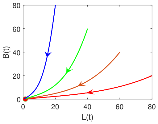
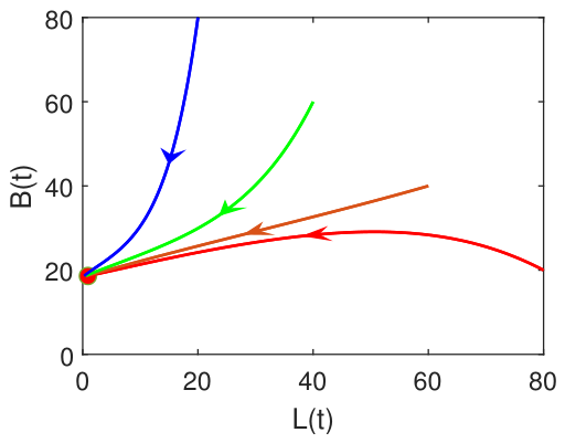
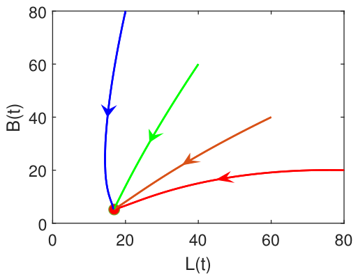
The experiments below illustrate the three local stability regimes. However, the nonlinearity in model (10) makes it difficult to analyze the global stability of this model. In what follows, some experiments are carried out to support the corresponding global convergence conjectures. In Figure 1, Figure 2 and Figure 3, the trajectories starting from (80, 20), (60, 40), (40, 60), and (20, 80) are represented by red, brown, green, and blue curves, respectively.

Experiment 1.

Let $\alpha =0.8$, $\mu =100$, $\delta =1$, ${\beta }_1=0.01$, ${\beta }_2=0.01$, ${\theta }_1=0.2$, ${\theta }_2=0.2$, $\eta =0.1$, and $\gamma =2$. These parameters give $R_0<1$, so Theorem 5 predicts local asymptotic stability of $E_0$. The trajectories in Figure 1 approach the virus-free state from several initial conditions.

Repeated tests over 1000 similar parameter sets support the following conjecture.

Conjecture 1.

If $R_0<1$, then the equilibrium $E_0$ is likely to be globally asymptotically stable in the feasible region.

Experiment 2.

Let $\alpha =0.8$, $\mu =100$, $\delta =0.1$, ${\beta }_1=0.0001$, ${\beta }_2=0.01$, ${\theta }_1=0.2$, ${\theta }_2=0.2$, $\eta =0.5$, and $\gamma =2$. Here $R_2>1$ and the quantities in Equations (54) and (56) satisfy $M_3<0$ and $M_5<0$. Theorem 6 shows convergence to the latency-free burst-endemic state.

The same numerical procedure suggests the following qualitative behavior.

Conjecture 2.

If $R_2>1$, $M_3<0$, and $M_5<0$, then $E_1$ is likely to be globally asymptotically stable in its feasible parameter region.

Experiment 3.

Let $\alpha =0.8$, $\mu =100$, $\delta =1$, ${\beta }_1=0.1$, ${\beta }_2=0.01$, ${\theta }_1=0.2$, ${\theta }_2=0.2$, $\eta =0.8$, and $\gamma =2$. In this case the coexistence equilibrium $E_2$ exists and the eigenvalues satisfy the fractional stability angle condition. The orbits shown in Figure 3 approach $E_2$.

The computations motivate the following conjecture.

Conjecture 3.

If $E_2$ exists and both eigenvalues in Equation (68) satisfy $|arg({\lambda }_i\left)\right|>\alpha \pi /2$, then $E_2$ is likely to be globally asymptotically stable in the feasible region.

9. Parameter Effects

This section makes further discussions. First, we analyze the sensitivity of the basic reproduction number to different parameters. Second, we examine the influence of the fractional order. Finally, we inspect the influence of the two saturation intensities.

9.1. Sensitivity of the Threshold

Normalized sensitivity is a dimensionless index that quantifies the relative change in a system’s output caused by a tiny relative perturbation of an input parameter. Unlike raw sensitivity, which carries physical units and cannot be fairly compared between parameters, normalized sensitivity removes unit and magnitude biases via scaling. For the purpose of analyzing the sensitivity of the basic reproduction number to different model parameters, we introduce the following notations:

(N1)

$S_{\mu }$: Normalized sensitivity of $R_0$ with respect to $\mu$; $S_{\mu }={\displaystyle \frac{\mu }{R_0}}{\displaystyle \frac{\partial R_0}{\partial \mu }}$.

(N2)

$S_{\delta }$: Normalized sensitivity of $R_0$ with respect to $\delta$; $S_{\delta }={\displaystyle \frac{\delta }{R_0}}{\displaystyle \frac{\partial R_0}{\partial \delta }}$.

(N3)

$S_{{\beta }_1}$: Normalized sensitivity of $R_0$ with respect to ${\beta }_1$; $S_{{\beta }_1}={\displaystyle \frac{{\beta }_1}{R_0}}{\displaystyle \frac{\partial R_0}{\partial {\beta }_1}}$.

(N4)

$S_{{\beta }_2}$: Normalized sensitivity of $R_0$ with respect to ${\beta }_2$; $S_{{\beta }_2}={\displaystyle \frac{{\beta }_2}{R_0}}{\displaystyle \frac{\partial R_0}{\partial {\beta }_2}}$.

(N5)

$S_{\eta }$: Normalized sensitivity of $R_0$ with respect to $\eta$; $S_{\eta }={\displaystyle \frac{\eta }{R_0}}{\displaystyle \frac{\partial R_0}{\partial \eta }}$.

(N6)

$S_{\gamma }$: Normalized sensitivity of $R_0$ with respect to $\gamma$; $S_{\gamma }={\displaystyle \frac{\gamma }{R_0}}{\displaystyle \frac{\partial R_0}{\partial \gamma }}$.

(N7)

$S_{{\theta }_1}$: Normalized sensitivity of $R_0$ with respect to ${\theta }_1$; $S_{{\theta }_1}={\displaystyle \frac{{\theta }_1}{R_0}}{\displaystyle \frac{\partial R_0}{\partial {\theta }_1}}$.

(N8)

$S_{{\theta }_2}$: Normalized sensitivity of $R_0$ with respect to ${\theta }_2$; $S_{{\theta }_2}={\displaystyle \frac{{\theta }_2}{R_0}}{\displaystyle \frac{\partial R_0}{\partial {\theta }_2}}$.

Theorem 8.

The following assertions hold.

(A1) 

If $R_1>R_2$, then $S_{\mu }=1$. If $R_1<R_2$, then $S_{\mu }=1$ as well.

(A2) 

If $R_1>R_2$, then $S_{\delta }=-{\displaystyle \frac{\eta +2\delta }{\eta +\delta }}$. If $R_1<R_2$, then $S_{\delta }=-{\displaystyle \frac{\gamma +2\delta }{\gamma +\delta }}$.

(A3) 

If $R_1>R_2$, then $S_{{\beta }_1}={\displaystyle \frac{\mu }{\delta (\eta +\delta )}}$. If $R_1<R_2$, then $S_{{\beta }_1}=0$.

(A4) 

If $R_1>R_2$, then $S_{{\beta }_2}=0$. If $R_1<R_2$, then $S_{{\beta }_2}={\displaystyle \frac{\mu }{\delta (\gamma +\delta )}}$.

(A5) 

If $R_1>R_2$, then $S_{\eta }=-{\displaystyle \frac{\delta }{\eta +\delta }}$. If $R_1<R_2$, then $S_{\eta }=0$.

(A6) 

If $R_1>R_2$, then $S_{\gamma }=0$. If $R_1<R_2$, then $S_{\gamma }=-{\displaystyle \frac{\delta }{\gamma +\delta }}$.

(A7) 

If $R_1>R_2$, then $S_{{\theta }_1}=0$. If $R_1<R_2$, then $S_{{\theta }_1}=0$.

(A8) 

If $R_1>R_2$, then $S_{{\theta }_2}=0$. If $R_1<R_2$, then $S_{{\theta }_2}=0$.

Proof of Theorem 8. 

The assertions follow through straightforward calculations. □

The following conclusions are drawn from the previous theorem.

(C1)

The entrance rate $\mu$ has a significant positive influence on the basic reproduction number $R_0$ if $R_1>R_2$ or $R_1<R_2$.

(C2)

The exit rate $\delta$ has a significant negative influence on $R_0$ if $R_1>R_2$ or $R_1<R_2$.

(C3)

The first infection force ${\beta }_1$ has a significant positive influence or has an influence on $R_0$ according to $R_1>R_2$ or $R_1<R_2$.

(C4)

The second infection force ${\beta }_2$ has no influence or has a significant positive influence on $R_0$ according to $R_1>R_2$ or $R_1<R_2$.

(C5)

The burst rate $\eta$ has a significant negative influence or has no influence on $R_0$ according to $R_1>R_2$ or $R_1<R_2$.

(C6)

The recovery rate $\gamma$ has no influence or has a significant negative influence on $R_0$ according to $R_1>R_2$ or $R_1<R_2$.

(C7)

The first saturation intensity ${\theta }_1$ has no influence on $R_0$ if $R_1>R_2$ or $R_1<R_2$.

(C8)

The second saturation intensity ${\theta }_2$ has no influence on $R_0$ if $R_1>R_2$ or $R_1<R_2$.

Remark 4.

$R_0$ is generally not differentiable at $R_1=R_2$. In this case, it is difficult to analyze the sensitivity of $R_0$ to model parameters. Fortunately, the probability of $R_1=R_2$ is negligible. Hence, it is reasonable to assume $R_1\ne R_2$.

9.2. Influence of the Fractional Order

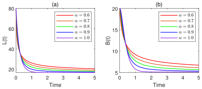
Experiment 4.

Let $\mu =100$, $\delta =1$, ${\beta }_1=0.1$, ${\beta }_2=0.01$, ${\theta }_1=0.2$, ${\theta }_2=0.2$, $\eta =0.8$, $\gamma =2$, $L\left(0\right)=80$, and $B\left(0\right)=20$. Take α from the set $A=\{0.6,0.7,0.8,0.9,1.0\}$. Figure 4 compares the time histories for different orders. It is observed that smaller α produces slower adjustment, which is consistent with the memory effect of the Caputo derivative.

Remark 5.

In this experiment, the fractional Adams predictor–corrector algorithm is performed when $\alpha <1$, whereas the second-order integer-order Adams predictor–corrector algorithm is performed when $\alpha =1$.

Across 1000 similar simulations, it is observed that decreasing the fractional order consistently slowed the evolution of both infected compartments.

9.3. Influence of the Saturation Intensities

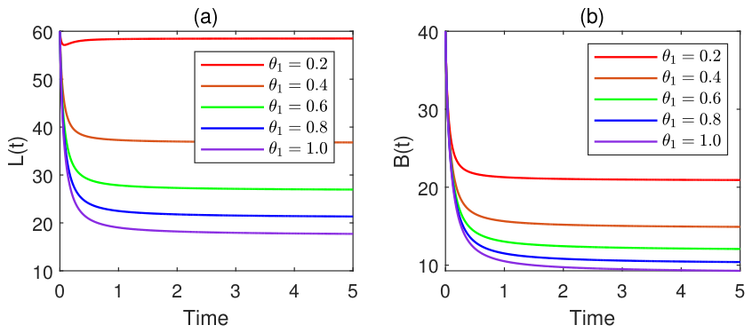
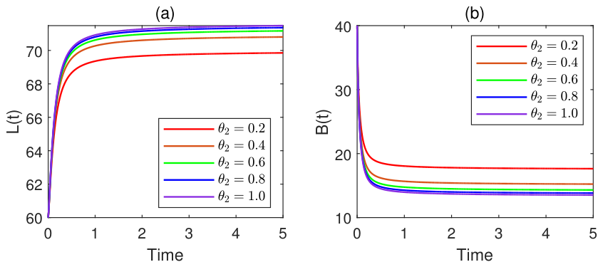
Experiment 5.

Let $\alpha =0.8$, $\mu =200$, $\delta =1$, ${\beta }_1=0.2$, ${\beta }_2=0.02$, $\eta =0.9$, $\gamma =2$, ${\theta }_2=0.2$, $L\left(0\right)=60$, and $B\left(0\right)=40$. Take ${\theta }_1$ from the set ${\mathsf{\Theta }}_1=\{0.2,0.4,0.6,0.8,1.0\}$. The trajectories in Figure 5 show how changing the latent-channel saturation coefficient alters the transient path and the final endemic levels.

Experiment 6.

Let $\alpha =0.8$, $\mu =200$, $\delta =1$, ${\beta }_1=0.2$, ${\beta }_2=0.04$, $\eta =0.5$, $\gamma =2$, ${\theta }_1=0.2$, $L\left(0\right)=60$, and $B\left(0\right)=40$. Take ${\theta }_2$ from the set ${\mathsf{\Theta }}_2=\{0.2,0.4,0.6,0.8,1.0\}$; Figure 6 gives the corresponding comparison for the bursting-channel saturation coefficient.

Through 1000 similar simulations, it is concluded that although ${\theta }_1$ and ${\theta }_2$ do not change the local threshold $R_0$, the experiments show that they can materially affect the speed of convergence and the endemic distribution between latent and bursting nodes.

10. Conclusions

A two-dimensional Caputo fractional SLBS model with two stage-specific Holling type-II infection functions has been developed and analyzed. The proposed formulation separates latent-driven and burst-driven transmission, which allows the two infected stages to have different strengths and different saturation mechanisms. The solution is non-negative, bounded, and well-posed for non-negative initial data. The system admits a threshold $R_0=max\{R_1,R_2\}$, a virus-free equilibrium, a possible latency-free burst-endemic equilibrium, and a possible coexistence equilibrium. Local stability criteria were obtained for all these equilibria through the fractional eigenvalue condition, and numerical simulations illustrated the resulting threshold behavior.

Several directions remain open. First, other nonlinear incidence functions, such as Beddington–DeAngelis or Monod–Haldane forms, may be introduced into fractional SLBS models [9,12,33,34,35,36]. Second, fractional CVP models would benefit from derivations based on stochastic processes or continuous-time random walks rather than from direct derivative replacement alone [37,38,39]. Third, the stage-specific approach used here may be adapted to other information-diffusion problems, including rumor propagation in social networks [40,41,42,43], immune surveillance of rumors [44,45], and batch reaction systems [46,47].

References

- Britton, N.F. Essential Mathematical Biology; Springer: Berlin/Heidelberg, Germany, 2003. [Google Scholar]
- Kephart, J.O.; White, S.R. Directed epidemiological models of computer viruses. In Proceedings of the 1999 IEEE Computer Society Symposium on Research in Security and Privacy, Los Alamitos, CA, USA, 20–22 May 1991; pp. 343–359. [Google Scholar]
- Kephart, J.O.; White, S.R. Measuring and modeling computer virus prevalence. In Proceedings of the 1999 IEEE Computer Society Symposium on Research in Security and Privacy, Los Alamitos, CA, USA, 24–26 May 1993; pp. 2–15. [Google Scholar]
- Piqueira, J.R.C.; Araujo, V.O. A modified epidemiological model for computer viruses. Appl. Math. Comput. 2009, 213, 355–360. [Google Scholar] [CrossRef]
- Toutonji, O.A.; Yoo, S.M.; Park, M. Stability analysis of VEISV propagation modeling for network worm attack. Appl. Math. Model. 2012, 36, 2751–2761. [Google Scholar] [CrossRef]
- Xiao, X.; Fu, P.; Dou, C.; Li, Q.; Hu, G.; Xia, S. Design and analysis of SEIQR worm propagation model in mobile internet. Commun. Nonlinear Sci. Numer. Simul. 2017, 43, 341–350. [Google Scholar] [CrossRef]
- Singh, A.; Awasthi, A.K.; Singh, K.; Srivastava, P.K. Modeling and analysis of worm propagation in wireless sensor networks. Wirel. Pers. Commun. 2018, 98, 2535–2551. [Google Scholar]
- Prakash, O.; Kumar, A.; Bharti, S.K. Computer virus propagation models: A mathematical review. J. Inf. Optim. Sci. 2023, 44, 1043–1055. [Google Scholar] [CrossRef]
- Upadhyay, R.K.; Kumari, S.; Misra, A.K. Modeling the virus dynamics in computer network with SVEIR model and nonlinear incident rate. J. Appl. Math. Comput. 2017, 54, 485–509. [Google Scholar]
- Upadhyay, R.K.; Kumari, S. Bifurcation analysis of an e-epidemic model in wireless sensor. Int. J. Comput. Math. 2018, 95, 1775–1805. [Google Scholar]
- MadhuSudanan, V.; Geetha, R. Dynamics of epidemic computer virus spreading model with delays. Wirel. Pers. Commun. 2020, 115, 2047–2061. [Google Scholar] [CrossRef]
- Zhang, Z.; Madhusudanan, V.; Murthy, B.S.N. Effect of delay in SMS worm propagation in mobile network with saturated incidence rate. Wirel. Pers. Commun. 2023, 131, 659–678. [Google Scholar] [CrossRef]
- Yang, L.; Yang, X. The spread of computer viruses under the influence of removable storage devices. Appl. Math. Comput. 2012, 219, 3914–3922. [Google Scholar] [CrossRef]
- Yang, L.; Yang, X.; Zhu, Q.; Wen, L. A computer virus model with graded cure rates. Nonlinear Anal. Real World Appl. 2013, 14, 414–422. [Google Scholar] [CrossRef]
- Yang, L.; Yang, X. A new epidemic model of computer viruses. Commun. Nonlinear Sci. Numer. Simul. 2014, 19, 1935–1944. [Google Scholar] [CrossRef]
- Ren, J.; Xu, Y. Stability and bifurcation of a computer virus propagation model with delay and incomplete antivirus ability. Math. Probl. Eng. 2014, 2014, 475934. [Google Scholar] [CrossRef]
- Yang, L.; Yang, X. The impact of nonlinear infection rate on the spread of computer virus. Nonlinear Dyn. 2015, 82, 85–95. [Google Scholar] [CrossRef]
- Zhao, T.; Wei, S.; Bi, D. Hopf bifurcation of a computer virus propagation model with two delays and infectivity in latent period. Syst. Sci. Control Eng. 2018, 6, 90–101. [Google Scholar] [CrossRef]
- Zhang, Z.; Kumari, S.; Upadhyay, R.K. A delayed e-epidemic SLBS model for computer virus. Adv. Differ. Equ. 2019, 2019, 414. [Google Scholar] [CrossRef]
- Li, C.; Liao, X. The impact of hybrid quarantine strategies and delay factor on viral prevalence in computer networks. Math. Model. Nat. Phenom. 2016, 11, 105–119. [Google Scholar] [CrossRef]
- Zhang, Z.; Upadhyay, R.K.; Bi, D.; Wei, R. Stability and Hopf bifurcation of a delayed epidemic model of computer virus with impact of antivirus software. Discret. Dyn. Nat. Soc. 2018, 2018, 8239823. [Google Scholar] [CrossRef]
- Ding, J.; Gul, N.; Liu, G.; Saeed, T. Dynamical aspects of a delayed computer viruses model with horizontal and vertical dissemination over internet. Fractals 2023, 31, 2340092. [Google Scholar] [CrossRef]
- Podlubny, I. Fractional Differential Equations; Academic Press: Cambridge, MA, USA, 1999. [Google Scholar]
- Zarin, R.; Khaliq, H.; Khan, A.; Khan, D.; Akgul, A.; Humphries, U.W. Deterministic and fractional modeling of a computer virus propagation. Results Phys. 2022, 33, 105130. [Google Scholar] [CrossRef]
- Sabir, Z.; Raja, M.A.Z.; Mumtaz, N.; Fathurrochman, I.; Sadat, R.; Ali, M.R. An investigation through stochastic procedures for solving the fractional order computer virus propagation mathematical model with kill signals. Neural Process. Lett. 2023, 55, 1783–1797. [Google Scholar]
- Zhou, Y.; Liu, B.; Zhou, K.; Shen, S. Malware propagation model of fractional order, optimal control strategy and simulations. Front. Phys. 2023, 11, 1201053. [Google Scholar] [CrossRef]
- Yang, L.; Song, Q.; Liu, Y. Dynamics analysis of a new fractional-order SVEIR-KS model for computer virus propagation: Stability and Hopf bifurcation. Neurocomputing 2024, 598, 128075. [Google Scholar] [CrossRef]
- Shi, X.; Luo, A.; Chen, X.; Huang, Y.; Huang, C.; Yin, X. The dynamical behaviors of a fractional-order malware propagation model in information networks. Mathematics 2024, 12, 3814. [Google Scholar] [CrossRef]
- Liu, Z.; Yang, X.; Yang, L. A fractional computer virus propagation model with saturation effect. Fractal Fract. 2025, 9, 587. [Google Scholar] [CrossRef]
- Diekmann, O.; Heesterbeek, J.A.P.; Metz, J.A.J. On the definition and the computation of the basic reproduction ratio R0 in models for infectious diseases in heterogeneous populations. J. Math. Biol. 1990, 28, 365–382. [Google Scholar] [CrossRef] [PubMed]
- van den Driessche, P.; Watmough, J. Reproduction numbers and sub-threshold endemic equilibria for compartmental models of disease transmission. Math. Biosci. 2002, 180, 29–48. [Google Scholar] [CrossRef] [PubMed]
- Diethelm, K.; Neville, J.; Ford, N.J.; Freed, A.D. A predictor-correction approach approach for the numerical solution of fractional differential equations. Nonlinear Dyn. 2002, 29, 3–22. [Google Scholar] [CrossRef]
- Zhao, T.; Zhang, Z.; Upadhyay, R.K. Delay-induced Hopf bifurcation of an SVEIR computer virus model with nonlinear incidence rate. Adv. Differ. Equ. 2018, 2018, 256. [Google Scholar] [CrossRef]
- Chu, Y.; Xia, W.; Wang, Z. A delayed computer virus model with nonlinear incidence rate. Syst. Sci. Control Eng. 2019, 7, 389–406. [Google Scholar] [CrossRef]
- Lu, H.; Zhu, E. A novel SIR-based computer virus propagation model with Beddington-DeAngelis functional response: Stability analysis and practical implications. AIMS Math. 2025, 10, 27412–27439. [Google Scholar] [CrossRef]
- Liu, J.; Saeed, T.; Zeb, A. Delay effect of an e-epidemic SEIRS malware propagation model with a generalized non-monotone incidence rate. Results Phys. 2022, 39, 105672. [Google Scholar] [CrossRef]
- Angstmann, C.N.; Henry, B.I.; McGann, A.V. A fractional-order infectivity SIR model. Phys. A 2016, 452, 8239823. [Google Scholar] [CrossRef]
- Angstmann, C.N.; Henry, B.I.; McGann, A.V. A fractional order recovery SIR model from a stochastic process. Bull. Math. Biol. 2016, 78, 468–499. [Google Scholar] [CrossRef] [PubMed]
- Angstmann, C.N.; Erickson, A.M.; Henry, B.I.; McGann, A.V.; Murray, J.M.; Nichols, J.A. A general framework for fractional order compartment models. SIAM Rev. 2021, 63, 375–392. [Google Scholar] [CrossRef]
- Singh, J. A new analysis for fractional rumor spreading dynamical model in a social network with Mittag-Leffler law. Chaos 2019, 29, 013137. [Google Scholar] [CrossRef] [PubMed]
- Yue, X.; Zhu, W. The dynamics and control of an ISCRM fractional-order rumor propagation model containing media reports. AIMS Math. 2024, 9, 9721–9745. [Google Scholar] [CrossRef]
- Wei, C.; Fu, C.; Yang, X.; Qin, Y.; Yang, L. Stability analysis of a rumor-spreading model with two time delays and saturation effect. Mathematics 2025, 13, 1729. [Google Scholar] [CrossRef] [PubMed]
- Niu, Y.; Muhammadhaji, A. Dynamics of a fractional-order IDSR rumor propagation model with time delays. Fractal Fract. 2025, 9, 242. [Google Scholar] [CrossRef]
- Swann, J.B.; Mark, J.S. Immune surveillance of tumors. J. Clin. Investig. 2007, 117, 1137–1146. [Google Scholar] [CrossRef] [PubMed]
- Baleanu, D.; Jajarmi, A.; Sajjadi, S.S.; Mozyrska, D. A new fractional model and optimal control of a tumor-immune surveillance with non-singular derivative operator. Chaos 2019, 29, 083127. [Google Scholar] [CrossRef] [PubMed]
- Wu, Y.; Ye, H.; Dong, H. A Multi-objective optimization for batch chemical reaction Processes: The trade-off between economy and safety. Chem. Eng. Sci. 2023, 265, 118231. [Google Scholar] [CrossRef]
- Chaudhary, K.K. A fractal-fractional dynamic model for batch reaction systems with instantaneous equilibrium: Theoretical analysis and numerical investigation. Chem. Eng. Sci. 2026, 335, 124453. [Google Scholar] [CrossRef]