ASPSO-Optimized RBF-IITSMC for High-Precision Trajectory Tracking of 6-DOF Robotic Arms Under Uncertainties

Abstract

To address high-precision trajectory tracking challenges in multi-joint robots facing model uncertainties, complex friction, and abrupt disturbances, this paper proposes a radial basis function (RBF) neural network-improved integral terminal sliding mode control scheme optimized by state-aware adaptive particle swarm optimization (ASPSO), denoted as ASPSO-optimized RBF-IITSMC. First, a fractional-memory integral terminal sliding surface incorporating a boundary-layer saturation mapping is constructed. The proposed terminal mapping is shown to be globally Lipschitz continuous, and an explicit approximation-error bound relative to the conventional terminal power mapping is established. Second, an RBF neural compensator driven by the sliding variable is incorporated into the reconstructed sliding dynamics to estimate lumped uncertainties and reduce the compensation burden on the robust feedback term. Furthermore, a state-aware adaptive PSO variant combining population-diversity monitoring and differential mutation is developed to jointly tune the 15-dimensional controller parameter vector. The practical finite-time reachability of the sliding variable and the uniform ultimate boundedness of the sliding variable and neural-weight estimation error are analyzed using a Lyapunov framework. Simulation results on a six-degree-of-freedom (6-DOF) robotic arm demonstrate improved tracking accuracy and disturbance-rejection performance, together with reduced high-frequency torque oscillations, compared with the evaluated baseline controllers.

1. Introduction

With the rapid development of intelligent manufacturing, six-degree-of-freedom (6-DOF) robotic arms have been widely used in medical assistance, aerospace, logistics, and human–robot collaboration [1,2,3]. Achieving high-precision trajectory tracking is the fundamental prerequisite for robotic arms to reliably execute complex tasks. To meet the increasingly stringent demands for control performance, scholars have proposed numerous advanced control strategies [4], such as robust control [5,6], impedance control [7], and time-delay estimation control [8]. However, achieving rapid and precise trajectory tracking remains a significant challenge. This difficulty primarily arises from the robotic arm’s highly nonlinear dynamics, parameter perturbations, strong coupling effects, and unknown external disturbances.

Sliding mode control (SMC) has been widely applied in the field of robot control due to its advantages of strong robustness, fast response, and concise design. However, the design of conventional sliding surfaces is limited, and the system is susceptible to parameter uncertainties, leading to high-frequency chattering and overshoot. To improve the convergence performance and tracking precision of system states, many scholars have conducted in-depth designs regarding the structural novelty of sliding surfaces. References [9,10] introduced fractional-order operators to handle variable loads, significantly improving the dynamic response characteristics of the system. References [11,12] proposed non-singular fixed-time terminal sliding surfaces, achieving a complete decoupling of the convergence time from the initial states. Reference [13] introduced a fractional-order fixed-time sliding surface equipped with a robust exact differentiator to optimize control efficacy. References [14,15] designed improved adaptive super-twisting sliding mode controllers that do not require an exact dynamic model, effectively smoothing the transient response of the system. Reference [16] employed an integral-type switching manifold to achieve highly efficient fault-tolerant trajectory tracking control for a quadrotor unmanned aerial vehicle (UAV) with parameter uncertainties. Reference [17] successfully applied a neural network integral terminal sliding mode control algorithm to the precise regulation of interaction forces in industrial robotic arms; Reference [18] constructed a fractional-order recurrent terminal sliding mode architecture combined with dynamic movement primitives to enhance transient quality; Reference [19] expounded a novel adaptive recurrent integral terminal sliding mode control strategy; Reference [20] developed a recurrent integral terminal sliding mode control (RITSMC) manifold topology, effectively overcoming the time-varying control challenges of a cable-driven continuum robot.

Aiming at the unknown nonlinearities and lumped uncertainties that are difficult to fully cover by the switching term of SMC, introducing intelligent approximation and observation compensation mechanisms, such as neural networks, has become a mainstream strategy to enhance closed-loop robustness. Reference [21] introduced an adaptive terminal sliding mode framework based on a radial basis function (RBF) network, achieving precise online compensation for dynamic errors. Reference [22] constructed a comprehensive anti-disturbance control topology integrating an RBF neural network disturbance observer. Reference [23] developed a neural network control system with adaptive weight updating. Aiming at complex constraint conditions, Reference [24] proposed a robot skill learning and generalized compensation method based on an adaptive neural network. Reference [25] constructed a closed-loop collaborative control system of a neural network and terminal sliding mode for a robotic arm, achieving robust trajectory tracking. Reference [26] combined non-singular global fast terminal sliding mode with an RBF neural network, effectively overcoming the model uncertainties and external disturbances faced by aerial robotic arms.

Swarm-intelligence algorithms have been widely studied for tuning the high-dimensional parameters of sliding surfaces, neural networks, and control laws. Reference [27] combined an improved particle swarm optimization (PSO) algorithm with a neural network high-order sliding mode architecture, significantly optimizing the control parameters. Reference [28] explored an optimal sliding mode control framework based on PSO under bounded disturbances. Reference [29] employed a genetic algorithm to dynamically adjust the parameters of a power reaching law to suppress torque oscillations. Furthermore, Reference [30] implemented a quantum particle swarm optimization (QPSO) algorithm to enhance the dynamic identification accuracy of a high-dimensional nonlinear robotic arm model. Reference [31] combined the PSO algorithm with a super-twisting non-singular sliding mode, achieving an optimal search for the control gain boundaries of an underwater robot. Reference [32] utilized a PSO algorithm to perform global dynamic optimization on the base width parameters of an adaptive local model approximation RBF neural network, significantly enhancing the anti-disturbance robustness and steady-state precision of an industrial robotic arm. References [33,34] successfully applied hybrid enhanced particle swarm optimization algorithms to the parameter tuning of complex vertical take-off and landing vehicles and multi-rotor systems.

Although the aforementioned advanced control architectures and intelligent optimization strategies have significantly advanced robotic trajectory tracking, critical limitations persist regarding their practical integration. First, despite the structural novelty of recent sliding manifolds, numerous methods remain dependent on conservative switching mechanisms to attenuate severe lumped disturbances. Consequently, achieving a practical trade-off between robust performance and control effort with reduced high-frequency oscillations remains challenging. Second, while sophisticated neural approximators have been extensively introduced, they frequently lack a streamlined architecture tailored specifically to sliding-mode dynamics. This results in structurally redundant compensators that impose significant computational overhead, thereby restricting high-frequency real-time execution. Finally, existing heuristic optimization frameworks in control design are typically confined to tuning a partial subset of parameters (e.g., only network weights or reaching laws). However, joint tuning across the coupled parameter space of a composite controller remains challenging. A research gap therefore remains in integrating smooth sliding-mode design, reduced-order neural compensation, and coordinated high-dimensional parameter tuning.

To address these issues, this paper develops an ASPSO-optimized RBF-IITSMC framework for high-precision trajectory tracking under lumped uncertainties. The mathematical contribution of this study lies in the quantitative characterization of the boundary-layer terminal mapping and the closed-loop formulation of the resulting composite controller. Specifically, its continuity, global Lipschitz property, approximation-error bound, and an explicit boundary-layer design interval are established. The reduced-order RBF compensator is formulated by separating the approximable component from the bounded residual, while ASPSO is employed as a numerical tool for jointly tuning the coupled controller parameters. Through numerical simulation experiments of a 6-DOF robotic arm in the MATLAB 2024b environment, the performance of the proposed composite control strategy in enhancing system robustness and steady-state precision is evaluated. The main technical and mathematical contributions of this paper can be summarized as follows:

(1)

An improved fractional-memory integral terminal sliding surface with boundary-layer regularization is developed. In addition to introducing the surface structure, the boundary-layer terminal mapping is analytically investigated. Its continuity and global Lipschitz property are established, and an explicit upper bound is derived for its approximation error relative to the conventional terminal power mapping. These results provide a quantitative interpretation of the relationship among the terminal exponent, boundary-layer thickness, approximation accuracy, and local feedback sensitivity.

(2)

An RBF neural compensator is incorporated into the reconstructed sliding dynamics to estimate the lumped matched uncertainty and reduce the compensation burden on the robust feedback term. The neural weight update law, approximation residual, and robust reaching action are included in a unified Lyapunov analysis, through which practical finite-time reachability of the sliding variable and uniform ultimate boundedness of the sliding variable and neural-weight estimation error are established under the stated assumptions.

(3)

A state-aware adaptive PSO variant is developed for the joint tuning of the 15-dimensional controller parameter vector. The normalized population-diversity index and stagnation information are used to adapt the swarm coefficients and activate differential mutation when premature convergence is detected. In contrast to tuning only an isolated subset of controller gains, the proposed implementation jointly considers the sliding-surface parameters, reaching-law gains, and neural adaptation gains under a composite index involving tracking error, transient response, and torque variation.

The remainder of this paper is organized as follows: Section 2 establishes the dynamic model of the 6-DOF robotic arm and provides the problem description of the error dynamics; Section 3 details the design and derivation process of the ASPSO-optimized RBF-IITSMC composite control law, the stability proof of the closed-loop system, and the implementation framework of the ASPSO algorithm; Section 4 presents comprehensive numerical simulation results and comparative analysis; finally, Section 5 summarizes the research conclusions of the entire paper.

2. Dynamic Modeling of the Robotic Arm

Considering a 6-DOF rigid serial robotic arm and neglecting the elastic deformation of its joints, the nonlinear dynamic model in the joint space is established using the Lagrange method as follows:

$$M\left(q\right)\ddot{q}+C\left(q,\dot{q}\right)\dot{q}+G\left(q\right)+F\left(q,\dot{q}\right)+{\tau }_d=\tau$$

(1)

where $q,\dot{q},\ddot{q}\in R^6$ denote the position, velocity, and acceleration vectors of the robotic arm in the joint space, respectively; $M\left(q\right)\in R^{6\times 6}$ is the symmetric positive-definite inertia matrix; $C(q,\dot{q})\in R^{6\times 6}$ is the centrifugal and Coriolis force matrix; $G\left(q\right)\in R^6$ is the gravity vector; $F\left(\dot{q}\right)\in R^6$ is the joint friction torque vector; ${\tau }_d\in R^6$ represents the unknown external disturbance vector; and $\tau \in R^6$ is the control input torque vector.

In practice, the actual dynamic model is typically decomposed into a nominal part and a parameter perturbation part:

$$\left\{\begin{array}{l}M(q)=M_0(q)+\Delta M(q)\hfill \\ C(q,\dot{q})=C_0(q,\dot{q})+\Delta C(q,\dot{q})\hfill \\ G(q)=G_0(q)+\Delta G(q)\hfill \end{array}\right.$$

(2)

where $M_0$, $C_0$, and $G_0$ are the nominal parameters of the model, and $\Delta M$, $\Delta C$, and $\Delta G$ denote the parameter perturbations. By substituting Equation (2) into the original dynamic model Equation (1) and rearranging the terms, the dynamic equation of the robotic arm system can be rewritten in the following form:

$$M_0\left(q\right)\ddot{q}+C_0\left(q,\dot{q}\right)\dot{q}+G_0\left(q\right)=\tau -X$$

(3)

where $X\in R^6$ is defined as the lumped uncertainty vector containing parameter perturbations, unmodeled friction, and external environmental disturbances, with its explicit expression given by:

$$X=\Delta M\left(q\right)\ddot{q}+\Delta C\left(q,\dot{q}\right)\dot{q}+\Delta G\left(q\right)+F\left(q,\dot{q}\right)+{\tau }_d$$

(4)

For the subsequent Lyapunov stability proof, the following standard assumption and properties are introduced:

Assumption 1. 

In practical systems, the joint velocity and acceleration of the robotic arm, as well as external environmental disturbances, are all bounded; therefore, the lumped uncertainty X is bounded. That is, there exists an unknown positive constant $\overline{X}>0$ such that its 2-norm satisfies $\Vert X\Vert \le \overline{X}$.

Property 1. 

The time derivative of the nominal inertia matrix, $M_0\left(q\right)$ and the nominal Coriolis matrix, $C_0\left(q,\dot{q}\right)$, satisfy a skew-symmetric relationship. Specifically, for any non-zero vector $\xi \in R^6$, the following equation holds identically:

$${\xi }^T({\dot{M}}_0(q)-2C_0(q,\dot{q}))\xi =0$$

(5)

Property 2. 

The nominal inertia matrix $M_0\left(q\right)$ is symmetric and positive definite. There exist known positive constants ${\kappa }_1$ and ${\kappa }_2$ such that for any vector $x\in R^6$, the following inequality holds:

$${\kappa }_1\Vert \mathrm{x}{\Vert }^2\le x^T{M}_0(q)x\le {\kappa }_2\Vert \mathrm{x}{\Vert }^2$$

(6)

Define $q_d\left(t\right)$ as the twice continuously differentiable desired trajectory. The position and velocity tracking errors are defined as:

$$e\left(t\right) = q\left(t\right) - q_d\left(t\right)$$

(7)

$$\dot{e}\left(t\right)=\dot{q}\left(t\right)-{\dot{q}}_d\left(t\right)$$

(8)

According to Equation (3), the actual joint acceleration $\ddot{q}$ can be expressed as:

$$\ddot{q}=M_0^{-1}\left(q\right)(\tau -C_0\left(q,\dot{q}\right)\dot{q}-G_0\left(q\right)-X)$$

(9)

Substituting this into the derivative equation of the tracking error yields the system error dynamics equation, which includes the control input and unknown disturbances:

$$\ddot{e}=M_0^{-1}\left(q\right)(\tau -C_0\left(q,\dot{q}\right)\dot{q}-G_0\left(q\right))-M_0^{-1}\left(q\right)X-{\ddot{q}}_d$$

(10)

3. Proposed Control Strategy Design

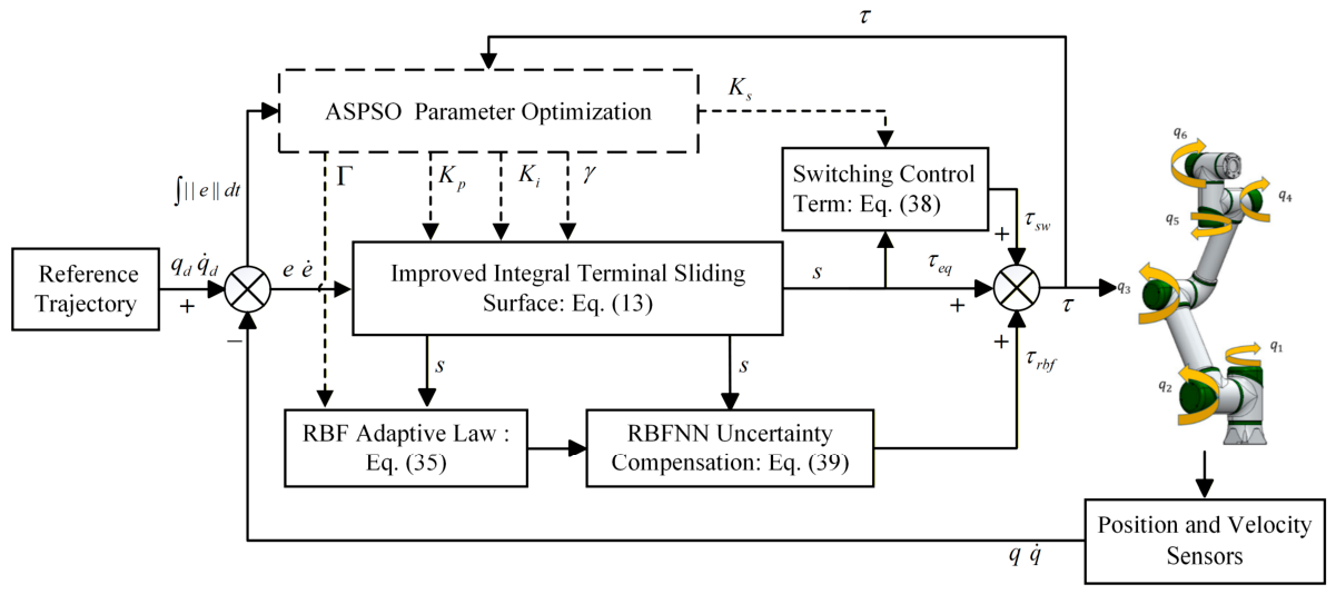
To achieve high-precision trajectory tracking for the 6-DOF collaborative robotic arm in the presence of model uncertainties and external disturbances, this paper proposes an ASPSO-optimized RBF-IITSMC scheme. The overall architecture of the control system is illustrated in Figure 1.

The control torque consists of an equivalent control term for compensating the nominal dynamics, an RBF neural compensation term for estimating the reduced-order approximable component of the lumped uncertainty, and a robust switching term for handling the remaining bounded residual and driving the system toward the prescribed sliding surface. Furthermore, the ASPSO algorithm is employed for offline joint tuning of the high-dimensional controller parameters, providing a numerical trade-off between tracking accuracy and torque smoothness.

3.1. Design of the Improved Integral Terminal Sliding Surface

In SMC, the selection of the sliding surface directly affects the transient response, steady-state accuracy, and convergence behavior of the system states. Integral terminal sliding mode control (ITSMC) introduces nonlinear terminal feedback into the integral channel and can provide finite-time convergence of the reduced-order error dynamics under appropriate gain and exponent conditions. Its standard sliding surface is defined as:

$$s_{ITSMC}=\dot{e}+{\displaystyle {\int }_0^t\left(K_p{\left|e\right|}^{{\alpha }_1}\mathrm{sgn}\left(e\right)+K_i{\left|\dot{e}\right|}^{{\alpha }_2}\mathrm{sgn}\left(\dot{e}\right)\right)}d\tau$$

(11)

where $s_{ITSMC}\in R^6$ is the ITSMC sliding surface vector; $K_p$ and $K_i$ are positive diagonal gain matrices; the constants ${\alpha }_1$ and ${\alpha }_2$ satisfy $0<{\alpha }_1<1$ and $0<{\alpha }_2<1$, respectively; and $\mathrm{sgn}(·)$ is the sign function. The absolute-value, fractional-power, and sign operations in Equation (11) are performed element-wise.

Although conventional ITSMC provides a terminal convergence mechanism, the discontinuous sign function embedded in it may induce high-frequency switching activity when the tracking error approaches the origin, resulting in oscillatory torque output and possible excitation of unmodeled high-frequency dynamics. To improve the continuity of the nonlinear error feedback, a boundary-layer saturation function is introduced. Meanwhile, the Riemann–Liouville (R–L) fractional-order integral operator is incorporated into the sliding surface to provide a tunable memory effect and frequency-dependent attenuation of the nonlinear feedback:

$${}_{0}D_t^{-\gamma }f(t)={\displaystyle \frac{1}{\mathrm{\Gamma }(\gamma )}}{\displaystyle {\int }_0^t{(t-\sigma )}^{\gamma -1}}f(\sigma )d\sigma$$

(12)

where ${}_{0}D_t^{-\gamma }$ denotes the R–L fractional integral operator of order $\gamma$, satisfying $0<\gamma <1$ and $\mathrm{\Gamma }(·)$ is the Gamma function. The positive convolution kernel assigns history-dependent weights to the nonlinear error feedback over the interval $\left[0,t\right]$.

Combining fractional-order calculus theory with the boundary-layer saturation function, the improved integral terminal sliding surface is designed as follows:

$$s=\dot{e}+{}_{0}D_t^{-\gamma }\left(K_p|e{|}^{{\alpha }_1}{\mathrm{sat}}_{{\Delta }_1}\left(e\right)+K_i|\dot{e}{|}^{{\alpha }_2}{\mathrm{sat}}_{{\Delta }_1}\left(\dot{e}\right)\right)$$

(13)

where $s\in R^6$ is the improved sliding mode variable. The operations of absolute value, fractional power, and saturation function in the equation are all performed element-wise.

To regularize the discontinuous sign mapping near the origin, this paper adopts a boundary-layer saturation function ${\mathrm{sat}}_{{\Delta }_1}(·)$ with ${\Delta }_1=0.001$, defined as follows:

$${\mathrm{sat}}_{{\Delta }_1}(x)=\left\{\begin{array}{ll}\mathrm{sgn}(x),\hfill & \left|x\right|>{\Delta }_1\hfill \\ {\displaystyle \frac{x}{{\Delta }_1}},\hfill & \left|x\right|\le {\Delta }_1\hfill \end{array}\right.$$

(14)

The saturation function regularizes the nonlinear feedback near the origin, whereas the fractional integral reshapes its temporal response through history-dependent weighting. The mathematical properties of the resulting boundary-layer terminal mapping are characterized below.

On the ideal sliding manifold, $s=0$, and the corresponding reduced-order error dynamics satisfy:

$$\dot{e}=-{}_{0}D_t^{-\gamma }(K_p|e{|}^{{\alpha }_1}{\mathrm{sat}}_{{\Delta }_1}(e)+K_i|\dot{e}{|}^{{\alpha }_2}{\mathrm{sat}}_{{\Delta }_1}(\dot{e}))$$

(15)

The following theorem characterizes the mathematical properties introduced by the boundary-layer modification.

Theorem 1. 

For $0<\alpha <1$ and $\Delta >0$, define the boundary-layer terminal mapping as ${\psi }_{\alpha ,\Delta }(x)=|x{|}^{\alpha }{\mathrm{sat}}_{\Delta }(x)$, and define the conventional terminal power mapping as ${\mathrm{sig}}_{\alpha }(x)=|x{|}^{\alpha }\mathrm{sgn}(x)$. Then, ${\psi }_{\alpha ,\Delta }(x)$ is continuous, odd, sign-preserving, and globally Lipschitz continuous. In particular,

$$\left|{\psi }_{\alpha ,\Delta }(x_1)-{\psi }_{\alpha ,\Delta }(x_2)\right|\le (\alpha +1){\Delta }^{\alpha -1}\left|x_1-x_2\right|$$

(16)

Moreover, the difference between the boundary-layer terminal mapping and the conventional terminal power mapping satisfies

$$\left|{\mathrm{sig}}_{\alpha }(x)-{\psi }_{\alpha ,\Delta }(x)\right|\le {\displaystyle \frac{{\alpha }^{\alpha }}{{(\alpha +1)}^{\alpha +1}}}{\Delta }^{\alpha }$$

(17)

Proof of Theorem 1. 

According to the definition of the saturation function, the boundary-layer terminal mapping can be written as

$${\psi }_{\alpha ,\Delta }(x)=\left\{\begin{array}{ll}|x{|}^{\alpha }\mathrm{sgn}(x),\hfill & \left|x\right|>\Delta \hfill \\ {\displaystyle \frac{|x{|}^{\alpha }x}{\Delta }},\hfill & \left|x\right|\le \Delta \hfill \end{array}\right.$$

(18)

The two expressions in Equation (18) have the same value at $x=\pm \Delta$. Therefore, ${\psi }_{\alpha ,\Delta }(x)$ is continuous. It is also odd and preserves the sign of $x$.

For $x\ne 0$, the magnitude of its derivative is

$${\displaystyle \frac{\mathrm{d}{\psi }_{\alpha ,\Delta }(x)}{\mathrm{d}x}}=\left\{\begin{array}{ll}\alpha |x{|}^{\alpha -1},\hfill & \left|x\right|>\Delta \hfill \\ {\displaystyle \frac{(\alpha +1)|x{|}^{\alpha }}{\Delta }},\hfill & 0<\left|x\right|<\Delta \hfill \end{array}\right.$$

(19)

For $\left|x\right|>\Delta$, the first expression in Equation (19) is no greater than $\alpha {\Delta }^{\alpha -1}$. For $0<\left|x\right|\le \Delta$, the second expression is no greater than $(\alpha +1){\Delta }^{\alpha -1}$. Hence, the derivative is globally bounded by $(\alpha +1){\Delta }^{\alpha -1}$, which proves Equation (16).

For $\left|x\right|>\Delta$, the two terminal mappings coincide, and their difference is zero. For $0<\left|x\right|\le \Delta$, let $r=\left|x\right|/\Delta \in [0,1]$. It follows that

$$\left|{\mathrm{sig}}_{\alpha }(x)-{\psi }_{\alpha ,\Delta }(x)\right|={\Delta }^{\alpha }{r}^{\alpha }(1-r)$$

(20)

The scalar function $r^{\alpha }(1-r)$ reaches its maximum at $r=\alpha /(\alpha +1)$, and

$${\max }_{r\in [0,1]}{r}^{\alpha }(1-r)={\displaystyle \frac{{\alpha }^{\alpha }}{{(\alpha +1)}^{\alpha +1}}}$$

(21)

Substituting Equation (21) into Equation (20) gives Equation (17). This completes the proof. □

Corollary 1. 

Given a prescribed maximum approximation error $E_{\max }>0$ and a prescribed maximum Lipschitz constant $L_{\max }>0$, the boundary-layer thickness $\Delta$ can be selected as:

$${\left({\displaystyle \frac{\alpha +1}{L_{\max }}}\right)}^{{\displaystyle \frac{1}{1-\alpha }}}\le \Delta \le {\left[{\displaystyle \frac{E_{\max }{(\alpha +1)}^{\alpha +1}}{{\alpha }^{\alpha }}}\right]}^{{\displaystyle \frac{1}{\alpha }}}$$

(22)

provided that the above interval is nonempty.

Proof of Corollary 1. 

According to Theorem 1, the certified Lipschitz constant and approximation-error bound are

$$L_{\psi }=(\alpha +1){\Delta }^{\alpha -1},\hspace{1em}{E}_{\psi }={\displaystyle \frac{{\alpha }^{\alpha }}{{(\alpha +1)}^{\alpha +1}}}{\Delta }^{\alpha }.$$

(23)

Solving $L_{\psi }\le L_{\max }$ and $E_{\psi }\le E_{\max }$ with respect to $\Delta$ gives Equation (22). □

Remark 1. 

Theorem 1 shows that the boundary-layer terminal mapping provides a globally Lipschitz regularization of the conventional terminal power mapping. Decreasing ${\Delta }_1$ reduces the approximation-error bound in Equation (17), but increases the Lipschitz bound in Equation (16). Corollary 1 converts this trade-off into an explicit interval for selecting the boundary-layer thickness under prescribed approximation-accuracy and feedback-sensitivity requirements.

Although Theorem 1 characterizes the regularity and approximation accuracy of the boundary-layer mapping, Equation (15) remains a nonlinear integro-differential equation with fractional memory. Therefore, the conventional integer-order convergence-time formula cannot be directly applied.

To exploit the structural properties of the nominal robotic-manipulator dynamics, the virtual reference velocity ${\dot{q}}_r\in R^6$ and virtual reference acceleration ${\ddot{q}}_r\in R^6$ are defined as:

$$s=\dot{q}-{\dot{q}}_r$$

(24)

$$\dot{s}=\ddot{q}-{\ddot{q}}_r$$

(25)

Under sufficient regularity and compatible initialization conditions, the R–L operators satisfy:

$${{\displaystyle \frac{d}{dt}}}_0{D}_t^{-\gamma }f{(t)}_0=D_t^{1-\gamma }f(t)$$

(26)

Combining Equations (13) and (24) gives:

$${\dot{q}}_r={\dot{q}}_d{-}_0{D}_t^{-\gamma }\left(K_p|e{|}^{{\alpha }_1}{\mathrm{sat}}_{{\Delta }_1}\left(e\right)+K_i|\dot{e}{|}^{{\alpha }_2}{\mathrm{sat}}_{{\Delta }_1}\left(\dot{e}\right)\right)$$

(27)

and

$${\ddot{q}}_r={\ddot{q}}_d{-}_0{D}_t^{1-\gamma }\left(K_p|e{|}^{{\alpha }_1}{\mathrm{sat}}_{{\Delta }_1}\left(e\right)+K_i|\dot{e}{|}^{{\alpha }_2}{\mathrm{sat}}_{{\Delta }_1}\left(\dot{e}\right)\right)$$

(28)

Substituting the reconstructed relationships into the robotic-manipulator dynamics yields:

$$M_0(q)\dot{s}+C_0(q,\dot{q})s=\tau -M_0(q){\ddot{q}}_r-C_0(q,\dot{q}){\dot{q}}_r-G_0(q)-X$$

(29)

Equation (29) retains the Coriolis cross-term $C_0(q,\dot{q})s$ on the left-hand side, thereby enabling direct use of the skew-symmetric property of the robotic-manipulator dynamics in the subsequent Lyapunov analysis.

3.2. RBF Neural Network Compensation Based on Sliding-Mode Variable Input

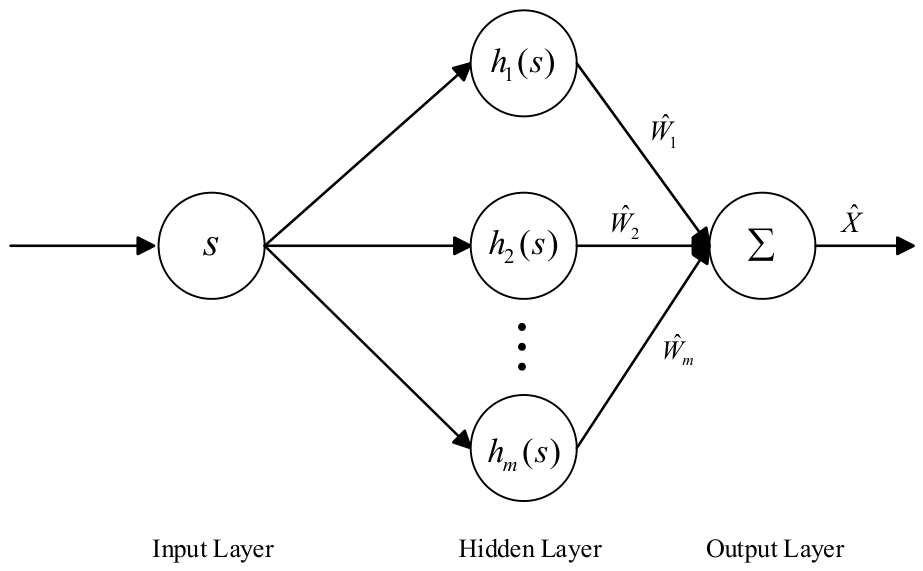
The lumped uncertainty includes state-dependent model perturbations, nonlinear friction, and external disturbances. To reduce the network input dimension, the sliding variable $s$ is employed as a reduced-order regressor over the considered compact operating region. The RBF network approximates the component correlated with the sliding dynamics, while the finite-node approximation error and reduced-order representation error are grouped into a bounded residual. The resulting network architecture is shown in Figure 2.

The estimated output $\widehat{X}$ of this network is defined as:

$$\widehat{X}={\widehat{W}}^{T}h\left(s\right)$$

(30)

where $\widehat{W}$ is the estimated weight matrix; $h(s)={[h_1(s),\dots ,h_m(s)]}^T$ is the Gaussian basis function vector, and the output of the $\mathrm{j}$-th node in the hidden layer is given by:

$$h_j(s)=\exp \left(-{\displaystyle \frac{\Vert s-c_j{\Vert }^2}{2b_j^2}}\right),\hspace{1em}j=1,\dots ,m$$

(31)

where $m$ is the total number of nodes in the hidden layer; $c_j$ and $b_j$ are the center vector and the width parameter of the Gaussian basis function, respectively.

According to the universal approximation property of RBF neural networks over the compact operating region ${\Omega }_s$, there exists an ideal constant weight matrix $W^{\ast }$ for the reduced-order approximable component $X_s\left(s\right)$, defined by

$$W^{\ast }=\arg {\min }_{W\in {\Omega }_W}\underset{s\in {\Omega }_s}{\sup }‖X_s(s)-W^{T}h(s)‖$$

(32)

Accordingly, the complete lumped uncertainty can be represented as

$$X(t)=W^{\ast T}h(s(t))+\epsilon (t)$$

(33)

where $\epsilon (t)$ denotes the total residual, including the finite-node RBF approximation error and the reduced-order representation error.

Remark 2. 

In Equation (33), ε is interpreted as the total residual associated with the reduced-order neural representation. It includes both the finite-node RBF approximation error and the representation error caused by using $s$ instead of the complete system state as the network input. Therefore, the use of the sliding variable as the sole regressor does not imply exact reconstruction of all heterogeneous uncertainty sources. The RBF network compensates for the component that is approximable from the sliding dynamics, whereas the remaining bounded residual is handled by the robust feedback term introduced in Section 3.3.

Assumption 2. 

There exists an unknown constant $\overline{\epsilon }>0$ such that the total residual satisfies:

$$\Vert \epsilon (t){\Vert }_2\le \overline{\epsilon }$$

(34)

To ensure the stability of the closed-loop system, the adaptive weight update law is designed as follows:

$$\dot{\widehat{W}}=-\mathrm{\Gamma }h(s)s^T-\sigma \mathrm{\Gamma }\widehat{W}$$

(35)

where $\mathrm{\Gamma }$ is a positive definite learning rate matrix. The leakage coefficient $\sigma$ is selected as a sufficiently small positive constant to prevent neural-weight drift caused by the nonzero approximation residual.

3.3. Design of the Composite Control Law

Based on the reconstructed error dynamics in Equation (29) and the RBF feedforward compensator, this paper designs a composite control law consisting of an equivalent control term, a switching control term, and a neural network compensation term. The control input torque $\tau \in R^6$ of the system is defined as follows:

$$\tau ={\tau }_{\mathrm{eq}}+{\tau }_{\mathrm{sw}}+{\tau }_{\mathrm{rbf}}$$

(36)

The equivalent control term is selected to cancel the known nominal dynamics in Equation (29), and is given by:

$${\tau }_{eq}=M_0(q){\ddot{q}}_r+C_0(q,\dot{q}){\dot{q}}_r+G_0(q)$$

(37)

To force the initial system state to rapidly reach the sliding surface within a finite time and to overcome partial residual unmodeled dynamics, this paper introduces a switching control strategy combined with an exponential reaching law. To reduce high-frequency switching activity induced by the conventional sign function $\mathrm{sgn}(·)$, this paper adopts a continuous saturation function ${\mathrm{sat}}_{{\Delta }_2}(·)$ with a boundary layer thickness of ${\Delta }_2=0.5$. The specific design of the switching control law is given by:

$${\tau }_{sw}=-M_0(q)\left(K_{s}s+K_r{\mathrm{sat}}_{{\Delta }_2}(s)\right)$$

(38)

where $K_s$ and $K_r$ are both positive gain matrices. The term $K_{s}s$ ensures that when the system state is far from the sliding surface, it can approach it rapidly at an exponential rate, while the ${\mathrm{sat}}_{{\Delta }_2}(·)$ term provides a continuous transition within the prescribed boundary layer of the control signal as the state penetrates the boundary layer.

In response to the lumped uncertainties that are difficult to acquire precisely during system operation, relying solely on increasing the switching gain $K_r$ to suppress disturbances would lead to conservative energy outputs and a risk of torque saturation. By utilizing the RBF neural network designed in Section 3.2 to perform online adaptive approximation and feedforward compensation, its compensation torque is designed as follows:

$${\tau }_{\mathrm{rbf}}=\widehat{X}={\widehat{W}}^{T}h(s)$$

(39)

The RBF compensation term estimates the reduced-order approximable component of the matched uncertainty, thereby reducing the compensation burden imposed on the robust switching term. The remaining bounded residual is handled by the robust feedback action, as clarified in Remark 3.

Remark 3. 

According to Equations (30) and (33), the uncertainty remaining after neural compensation can be expressed as $\tilde{X}=X-\widehat{X}={\tilde{W}}^{T}h(s)+\epsilon$, where $\tilde{W}=W^{\ast }-\widehat{W}$. The adaptive law addresses the weight-estimation term in the stability analysis, whereas the robust feedback term handles the bounded residual l $\epsilon$. Thus, the switching gain need not be selected solely according to the bound of the complete lumped uncertainty.

Integrating the aforementioned designs and substituting the equivalent control, switching control, and neural network compensation terms uniformly into the overall equation, the composite control law proposed in this paper can be expressed as:

$$\tau =M_0(q)\left({\ddot{q}}_r-K_{s}s-K_r{\mathrm{sat}}_{\Delta }(s)\right)+C_0(q,\dot{q}){\dot{q}}_r+G_0(q)+{\widehat{W}}^{T}h(s)$$

(40)

3.4. Stability Analysis

To account for the matrix coupling introduced by the inertia-weighted reaching law, the following condition is imposed.

Assumption 3. 

Let $Q$ denote the compact joint-position operating region. Define

$$Q_s(q)={\displaystyle \frac{1}{2}}\left[M_0(q)K_s+K_s{M}_0(q)\right]$$

(41)

$$A_r(q)=M_0(q)K_r=\left[a_{ij}(q)\right]$$

(42)

There exist constants ${\mu }_s>0$, $d_r>0$, and ${\overline{a}}_r>0$ such that, for all $q\in \mathcal{Q}$,

$$Q_s(q)\succcurlyeq {\mu }_{s}I$$

(43)

$$a_{ii}(q)-{\displaystyle \sum _{j\ne i}\left|a_{ij}(q)\right|}\ge d_r, i=1,\dots ,6$$

(44)

$${\displaystyle \sum _{i=1}^6{a}_{ii}}(q)\le {\overline{a}}_r$$

(45)

Lemma 1. 

Under Assumption 3, the inertia-weighted boundary-layer term satisfies:

$$s^T{A}_r(q){\mathrm{sat}}_{{\Delta }_2}(s)\ge d_r\Vert s{\Vert }_1-{\displaystyle \frac{{\overline{a}}_r{\Delta }_2}{4}}$$

(46)

Proof of Lemma 1. 

For any $x\in R$,

$$x{\mathrm{sat}}_{\Delta }(x)\ge |x|-{\displaystyle \frac{\Delta }{4}}$$

(47)

For $|x|\le \Delta$, this follows from

$${\displaystyle \frac{|x{|}^2}{\Delta }}-|x|+{\displaystyle \frac{\Delta }{4}}={\displaystyle \frac{1}{\Delta }}{\left(|x|-{\displaystyle \frac{\Delta }{2}}\right)}^2\ge 0,$$

(48)

Expanding $s^{T}A(q){\mathrm{sat}}_{{\mathsf{\Delta }}_2}(s)$, and using Equation (47), $\left|{\mathrm{sat}}_{{\Delta }_2}(s_j)\right|\le 1$, and conditions (44), yields Equation (46). □

Theorem 2. 

Consider the robotic-manipulator system described by Equation (3). Under the composite control law in Equation (40) and the adaptive weight update law in Equation (35), suppose that

$$d_r>\overline{\epsilon }$$

(49)

where $\overline{\epsilon }$ is the total residual bound in Assumption 2. Then $s$ and $\tilde{W}=W^{\ast }-\widehat{W}$ are uniformly ultimately bounded. Moreover, under the condition derived below, $s$ enters the prescribed component-wise boundary layer within a finite time and remains inside it thereafter.

Proof of Theorem 2. 

Substituting the composite control law into the reconstructed sliding dynamics yields:

$$M_0(q)\dot{s}+C_0(q,\dot{q})s=-M_0(q)K_{s}s-M_0(q)K_r{\mathrm{sat}}_{{\Delta }_2}(s)-{\tilde{W}}^{T}h(s)-\epsilon$$

(50)

Consider the Lyapunov function:

$$V={\displaystyle \frac{1}{2}}{s}^T{M}_0(q)s+{\displaystyle \frac{1}{2}}\mathrm{tr}\left({\tilde{W}}^T{\mathrm{\Gamma }}^{-1}\tilde{W}\right)$$

(51)

Using Property 1 and the adaptive law in Equation (35), the derivative of $V$ becomes:

$$\dot{V}=-s^T{M}_0(q)K_{s}s-s^T{A}_r(q){\mathrm{sat}}_{{\Delta }_2}(s)-s^T\epsilon +\sigma \mathrm{tr}\left({\tilde{W}}^T\tilde{W}\right).$$

(52)

Since the ideal weight matrix $W^{\ast }$ is constant and finite over the considered compact operating region, its Frobenius norm is bounded by a positive constant $\overline{W}$. Using $\tilde{W}=W^{\ast }-\widehat{W}$ and Young’s inequality:

$$\mathrm{tr}\left({\tilde{W}}^T\tilde{W}\right)\le -{\displaystyle \frac{1}{2}}\Vert \tilde{W}{\Vert }_F^2+{\displaystyle \frac{1}{2}}{\overline{W}}^2.$$

(53)

Furthermore:

$$s^T{M}_0(q)K_{s}s=s^T{Q}_s(q)s\ge {\mu }_s\Vert s{\Vert }_2^2$$

(54)

Combining Assumptions 2 and 3, and Lemma 1 gives:

$$\dot{V}\le -{\mu }_s\Vert s{\Vert }_2^2-\delta \Vert s{\Vert }_2-{\displaystyle \frac{\sigma }{2}}\Vert \tilde{W}{\Vert }_F^2+C$$

(55)

where

$$\delta =d_{\tau }-\overline{\epsilon }>0,\hspace{1em}C={\displaystyle \frac{{\overline{a}}_{\tau }{\Delta }_2}{4}}+{\displaystyle \frac{\sigma }{2}}{\overline{W}}^2$$

(56)

Because:

$$V\le {\displaystyle \frac{{\kappa }_2}{2}}\Vert s{\Vert }_2^2+{\displaystyle \frac{{\lambda }_{\max }\left({\mathrm{\Gamma }}^{-1}\right)}{2}}\Vert \tilde{W}{\Vert }_F^2$$

(57)

Define:

$$\lambda =\min \left\{{\displaystyle \frac{2{\mu }_s}{{\kappa }_2}}, {\displaystyle \frac{\sigma }{{\lambda }_{\max }\left({\mathrm{\Gamma }}^{-1}\right)}}\right\}>0$$

(58)

After omitting the non-positive term $-\delta \Vert s{\Vert }_2$, Equation (55) becomes:

$$\dot{V}\le -\lambda V+C$$

(59)

Thus:

$$V(t)\le {\displaystyle \frac{C}{\lambda }}+\left(V(0)-{\displaystyle \frac{C}{\lambda }}\right)e^{-\lambda t}$$

(60)

Which proves uniform ultimate boundedness of $s$ and $\tilde{W}$.

For any $\zeta >0$,define:

$${\Omega }_{\zeta }=\left\{\left(s,\tilde{W}\right):V\le {\displaystyle \frac{C}{\lambda }}+\zeta \right\}$$

(61)

On its boundary:

$$\dot{V}\le -\lambda \left({\displaystyle \frac{C}{\lambda }}+\zeta \right)+C=-\lambda \zeta <0$$

(62)

So ${\Omega }_{\zeta }$ is positively invariant. If the initial state is outside this set, it enters ${\Omega }_{\zeta }$ within:

$$T_{\zeta }\le {\displaystyle \frac{1}{\lambda }}\ln \left({\displaystyle \frac{V(0)-C/\lambda }{\zeta }}\right)$$

(63)

If:

$${\displaystyle \frac{C}{\lambda }}+\zeta \le {\displaystyle \frac{{\kappa }_1{\Delta }_2^2}{2}}$$

(64)

Then $V\ge {\displaystyle \frac{{\kappa }_1\Vert s{\Vert }_2^2}{2}}$ implies:

$$\Vert s_i(t)\Vert \le \Vert s(t){\Vert }_2\le {\Delta }_2,\hspace{1em}i=1,\dots ,6, \forall t\ge T_{\zeta }$$

(65)

Therefore, the sliding variable enters the prescribed component-wise boundary layer within a finite time and remains inside it thereafter. □

Corollary 2. 

Under the conditions of Theorem 2, the excess Lyapunov function above the ultimate level $c/\lambda$ satisfies:

$${\left[V(t)-{\displaystyle \frac{C}{\lambda }}\right]}_{+}\le e^{-\lambda t}{\left[V(0)-{\displaystyle \frac{C}{\lambda }}\right]}_{+}$$

(66)

where ${[x]}_{+}=max\{x,0\}$. Therefore, the excess above the ultimate bound decays exponentially with the certified rate parameter $\lambda$. For any $\zeta >0$, the trajectory enters the set ${\mathsf{\Omega }}_{\zeta }$ defined in Equation (61) within the time estimated in Equation (63).

Proof of Corollary 2. 

The result follows directly by subtracting $C/\lambda$ from both sides of Equation (60) and applying the positive-part operator. □

Remark 4. 

The parameters ${\mu }_s$, $d_r-\overline{\epsilon }$, and $c_{\Delta }$ explicitly determine the practical stability region. The σ-modification prevents neural-weight drift and produces the negative-definite weight-error term required for uniform ultimate boundedness. Condition (64) guarantees finite-time entrance into and subsequent confinement within the prescribed boundary layer. Corollary 2 further quantifies the exponential approach to the ultimate set with the decay-rate parameter λ.

3.5. State-Aware Adaptive PSO for Joint Controller-Parameter Tuning

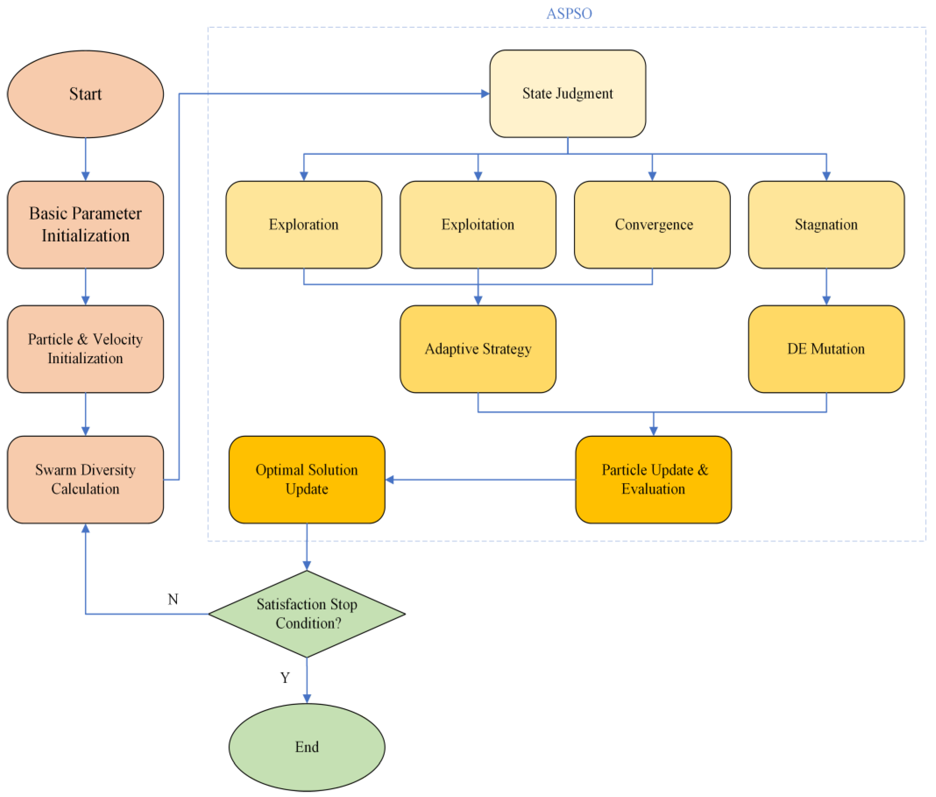
The dynamic response performance of the composite controller is highly dependent on the appropriate configuration of the gain parameters. Traditional manual trial-and-error methods struggle to cope with the high-dimensional parameter space brought about by multi-joint heterogeneous dynamics, whereas the standard PSO algorithm is prone to falling into local optima when handling high-dimensional objectives due to the premature loss of population diversity. To address this parameter-tuning problem, this paper employs a state-aware adaptive PSO variant, whose execution procedure is illustrated in Figure 3.

Combining the algorithm execution framework in Figure 3, the ASPSO achieves joint parameter optimization of the high-dimensional controller parameters through three core mechanisms: population initialization, evolutionary state identification, and dual-branch dynamic evolution. In the initialization phase, the algorithm first randomly generates an initial population of size $N$ within the predefined parameter search space and assigns initial positions and velocities to each particle.

The core parameters to be optimized in the proposed scheme total 15 dimensions. The position vector $x_i\left(t\right)$ of each particle represents a set of 15-dimensional candidate solutions, mathematically defined as $x_i=\left[K_p,K_i,\gamma ,K_{s1},\dots ,K_{s6},{\mathrm{\Gamma }}_1,\dots ,{\mathrm{\Gamma }}_6\right]$. In this vector, the proportional gain $K_p$, the integral gain $K_i$, and the fractional order $\gamma$ are one-dimensional scalar parameters, while $K_{s1\dots 6}$ and ${\mathrm{\Gamma }}_{1\dots 6}$ correspond to the main diagonal elements of the switching reaching law gain matrix $K_s$ and the RBF neural network learning rate matrix $\mathrm{\Gamma }$, respectively.

During the evolutionary process, the state-aware mechanism is the key to the algorithm reducing the risk of premature stagnation. The algorithm calculates the mean squared Euclidean distance from all particles to the geometric centroid of the population according to the following equation, thereby quantifying the population diversity $D\left(t\right)$ at the current iteration $t$:

$$D(t)={\displaystyle \frac{1}{N}}{\displaystyle \sum _{i=1}^N{‖x_i(t)-\overline{x}(t)‖}^2}$$

(67)

where $\overline{x}(t)$ is the geometric centroid of the particle swarm at the current iteration, and $N$ is the total number of particles. To perceive the relative state of the current evolution, a normalized diversity index $\Delta (t)$ is defined as the ratio of the current diversity to the historical maximum diversity:

$$\Delta (t)={\displaystyle \frac{D(t)}{{\max }_{1\le \tau \le t}D(\tau )}}$$

(68)

On this basis, by introducing state division thresholds ${\delta }_{\mathrm{high}}$ and ${\delta }_{\mathrm{low}}$, along with a stagnation counter $k_{\mathrm{stall}}$, the swarm is classified into four evolutionary states. The specific logical judgment mechanism is as follows: when the normalized diversity index satisfies $\Delta (t)>{\delta }_{\mathrm{high}}$, the system is in the exploration state, prioritizing broader exploration; when ${\delta }_{\mathrm{low}}<\Delta (t)\le {\delta }_{\mathrm{high}}$, the system transitions into the exploitation state to perform refined local search; if $\Delta (t)\le {\delta }_{\mathrm{low}}$ and $k_{\mathrm{stall}}<k_{\mathrm{limit}}$, it is determined as the convergence state; whereas when $\Delta (t)\le {\delta }_{\mathrm{low}}$ and $k_{\mathrm{stall}}\ge k_{\mathrm{limit}}$, it indicates that the population has lost its diversity and fallen into a stagnation state.

Based on the aforementioned topological state identification results, the algorithm activates a dual-branch dynamic evolution mechanism to perform individual updates. If determined to be in the exploration, exploitation, or convergence state, the algorithm triggers the adaptive evolution branch, constructing the following adaptive evolution equations in which the inertia weight $\omega (t)$ and the learning factors $c_1(t)$ and $c_2(t)$ are dynamically adjusted along with $\Delta (t)$:

$$\left\{\begin{array}{l}\omega (t)={\omega }_{\min }+({\omega }_{\max }-{\omega }_{\min })·\Delta (t)\hfill \\ c_1(t)=c_{1,\max }-(c_{1,\max }-c_{1,\min })·\exp (-\Delta (t))\hfill \\ c_2(t)=c_{2,\min }+(c_{2,\max }-c_{2,\min })·\exp (\Delta (t)-1)\hfill \end{array}\right.$$

(69)

where ${\omega }_{\max }$ and ${\omega }_{\min }$ are the maximum and minimum values of the inertia weight, respectively; $c_{1,\max }$, $c_{1,\min }$ and $c_{2,\max }$, $c_{2,\min }$ correspond to the value boundaries of the individual learning factor and the social learning factor, respectively. Furthermore, the standard velocity equation expressed below is utilized to achieve an adaptive transition from search breadth to search depth:

$$v_i^{t+1}=\omega v_i^t+c_1{r}_1\left(p_{\mathrm{best},i}^t-x_i^t\right)+c_2{r}_2\left(g_{\mathrm{best}}^t-x_i^t\right)$$

(70)

where $v_i^t$ is the particle velocity; $r_1$ and $r_2$ are random numbers in the interval $[0,1]$; $p_{\mathrm{best},i}^t$ and $g_{\mathrm{best}}^t$ are the historical personal best position of the individual and the global best position of the population, respectively. Once the system is detected to have fallen into a stagnation state, the algorithm immediately switches to the DE mutation branch, executing the following differential evolution mutation operation on the bottom 40% of the non-elite individuals based on fitness ranking:

$$x_{i,new}=x_{r1}+F·(x_{r2}-x_{r3})$$

(71)

where $x_{i,new}$ is the new particle position generated after mutation; $x_{r1}$, $x_{r2}$, and $x_{r3}$ are mutually distinct particle positions randomly selected from the population; and $F$ is the scaling factor. By reshaping population diversity, this mutation operation effectively assists the particle swarm in reducing the risk of premature stagnation.

After each particle update, the candidate solutions are evaluated using the composite cost function in Equation (72). To comprehensively balance trajectory tracking precision, control torque smoothness, and transient response performance, the following composite cost function to be minimized is constructed:

$$J=w_1{J}_{\mathrm{SSE}}+w_2{J}_{\mathrm{Smooth}}+w_3{J}_{\mathrm{Overshoot}}+w_4{J}_{\mathrm{Time}}$$

(72)

where $J_{\mathrm{SSE}}={\displaystyle \sum {\displaystyle {\int }_{t_{\mathrm{ss}}}^T\parallel e(t){\parallel }^2}}dt$ is the steady-state error integral, used to eliminate static tracking errors; $J_{\mathrm{Smooth}}={\displaystyle \sum |}\Delta \tau |$ is the high-frequency chattering penalty term, aiming to guarantee the continuity of the control signal; $J_{\mathrm{Overshoot}}$ and $J_{\mathrm{Time}}$ represent the overshoot penalty term and the settling time penalty term during the position tracking process, respectively; and $w_1$, $w_2$, $w_3$, and $w_4$ are the corresponding weighting coefficients for each term. The algorithm substitutes the updated particles into this cost function to re-evaluate their fitness, synchronously updating the historical personal best $p_{\mathrm{best}}$ and the global best $g_{\mathrm{best}}$, until the termination condition is met and the best-found 15-dimensional controller parameter vector under the specified computational settings is returned.

4. Simulation and Analysis

To verify the effectiveness and robustness of the proposed ASPSO-optimized RBF-IITSMC control strategy in dealing with model uncertainties, complex friction, and abrupt external disturbances, numerical simulations are conducted taking the VSCR-6CUR3 6-DOF collaborative robotic arm (VSTC, Hefei, China) as the research object.

4.1. Simulation Platform and Experimental Setup

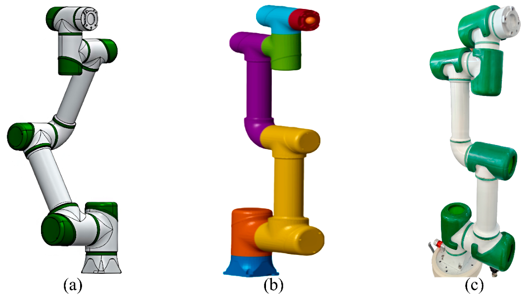
The simulations are carried out in the MATLAB/Simulink (version R2024b, MathWorks, Natick, MA, USA) environment. The solver adopts the fixed-step ode3, with the integration step size set to 0.0001 s. A 3D solid model is imported into Simscape Multibody to represent the coupled nonlinear dynamics of the robotic arm. Figure 4 shows the model, and

Table 1. Dynamic parameters of the 6-DOF robotic arm.

Parameter	Symbol	Link 1	Link 2	Link 3	Link 4	Link 5	Link 6
Mass (kg)	m	2.5439	5.8003	2.6264	0.9560	0.9560	0.5914
Center of Mass (cm)	$lcx$	0.0072	−13.0740	−15.2883	0.0099	−0.0099	0.0001
	$lcy$	−0.2993	−0.0069	−0.0215	−0.0337	0.0337	−0.0025
	$lcz$	−1.1171	−0.7482	0.3729	−0.2771	−0.2771	−1.7039
Inertia (kg·cm2)	$Ixx$	49.1124	87.9041	25.1069	10.3748	10.3748	4.2615
	$Iyy$	47.7647	2050.8634	959.8324	5.7841	5.7841	4.2744
	$Izz$	28.3380	2016.7923	953.9071	9.9633	9.9633	4.0058

lists the main link parameters. To address the computational overhead induced by the infinite memory characteristic of the fractional-order calculus operator, an improved Oustaloup filter is employed for frequency-domain approximation, with the effective frequency band set to [0.001, 1000] rad/s and the approximation order set as $N=5$.

The desired reference trajectories for all joints are uniformly set as $q_{di}=\cos (t)[\mathrm{rad}]$ $(\mathrm{i}=1,\dots ,6)$. To comprehensively evaluate the controller performance, the following lumped uncertainties and time-varying external disturbances are introduced into the simulation:

• Parameter perturbations and nonlinear friction: A 20% parameter perturbation is intentionally injected based on the nominal dynamic model, and the joint nonlinear friction is modeled as $F_{fi}({\dot{q}}_i)=0.1\mathrm{sgn}({\dot{q}}_i)+2{\dot{q}}_i[\mathrm{N}·\mathrm{m}]\hspace{1em}(\mathrm{i}=1,\dots ,6)$
• Composite external disturbances: Continuous time-varying nonlinear disturbances ${\tau }_{di}=3\sin (t)[\mathrm{N}·\mathrm{m}]\hspace{1em}(i=1,\dots ,6)$ are applied to all joints. In addition, to simulate extreme operating conditions such as physical collisions or sudden load variations, step impact signals with amplitudes of $[10, 10, 10, 1, 0.3, 0.1] [\mathrm{N}·\mathrm{m}]$ are respectively injected into joints 1 through 6 at $t=5\mathrm{s}$

To conduct a rigorous comparative analysis and evaluate against advanced baseline methods, four sets of control schemes are designed. Structurally, except for the ST-ITSMC—which utilizes its inherent super-twisting algorithm—the switching control laws of the remaining schemes all adopt the exponential reaching law combined with a saturation function. Furthermore, to ensure comparative validity and mitigate configuration bias, the three baseline controllers were systematically tuned manually to achieve their best empirical performance. In contrast, the parameters of the proposed method were autonomously optimized by the ASPSO algorithm. The specific schemes are defined as follows:

• ITSMC: This scheme adopts the conventional integer-order integral sliding surface defined by Equation (11).
• ST-ITSMC: This scheme combines the conventional integer-order integral sliding surface defined by Equation (11) with a super-twisting reaching law. As a robust second-order sliding mode baseline, it effectively mitigates chattering while preserving finite-time convergence.
• RBF-IITSMC: An RBF neural network is introduced to perform online approximation and compensation for the lumped uncertainties, adopting the composite control law Equation (40). All gain parameters of this controller are assigned fixed values based on manual experience, without employing a parameter optimization algorithm.
• Proposed Method (ASPSO-optimized RBF-IITSMC): The scheme proposed in this paper. Based on the RBF-IITSMC architecture, the ASPSO algorithm is employed to perform offline joint optimization on the 15-dimensional core control parameters, achieving a numerical trade-off between tracking precision and torque smoothness.

In the ASPSO implementation, the population size $N$ and the maximum number of iterations $T_{max}$ are set to 60 and 30, respectively. These values are heuristically selected according to the 15-dimensional search space to balance exploration capability and computational efficiency. The evolutionary-state thresholds are set to ${\delta }_{\mathrm{high}}=0.7$ and ${\delta }_{\mathrm{low}}=0.3$, which divide the normalized diversity index into exploration, exploitation, and low-diversity regions.

The weights of the composite cost function are selected according to control-objective priority and magnitude normalization, since the four performance indices have substantially different numerical scales. Specifically, the steady-state tracking-error weight is set to $w_1=3000$ to preserve sufficient sensitivity to the small residual errors occurring in the later optimization stage. The torque-variation weight is set to $w_2=0.02$ to account for the relatively large numerical magnitude of the smoothness term and to balance tracking accuracy against torque oscillation. The overshoot and settling-time weights are set to $w_3=150$ and $w_4=50$, respectively, to constrain the transient response.

The detailed parameter settings are summarized in

Table 2. Parameter configurations for the composite controller and ASPSO algorithm.

Description	Symbol	Value
Optimized Controller Parameters	${\alpha }_1$, ${\alpha }_2$, ${\Delta }_1$, ${\Delta }_2$	0.5, 0.5, 0.001, 0.5
	$K_p$, $K_i$, $\gamma$	6.94, 11.38, 0.95
	$K_s$, $K_r$	diag(14.39, 29.82, 47.03, 89.27, 120.00, 149.75), 1
	$\mathrm{\Gamma }$, $\sigma$	diag(149.40, 301.29, 91.00, 29.00, 10.59, 2.96), 0.01 [−1.63, −1.06, −0.68, −0.45, −0.3, −0.047, −0.024, −0.0001, 0.023, 0.05, 0.18, 0.48], 12
	$c_j$, m
ASPSO Hyperparameters	$N$, $T_{max}$ ${\delta }_{\mathrm{high}}$ ${\delta }_{\mathrm{low}}$, $k_{\mathrm{limit}}$	60, 30 0.7, 0.3, 5
	$w_1$, $w_2$, $w_3$, $w_4$	3000, 0.02, 150, 50

. The controller gains reported in the table are not manually assigned; they are the best-found parameter values obtained from the reported ASPSO runs under the specified computational settings.

4.2. Simulation Results and Discussion

To verify the effectiveness and robustness of the proposed ASPSO-optimized RBF-IITSMC control strategy in handling model uncertainties, complex friction, and abrupt external disturbances, this section comparatively evaluates the numerical simulation results of the ITSMC, the ST-ITSMC, the fixed-parameter RBF-IITSMC, and the ASPSO-optimized RBF-IITSMC.

4.2.1. Trajectory Tracking Performance and Steady-State Error Analysis

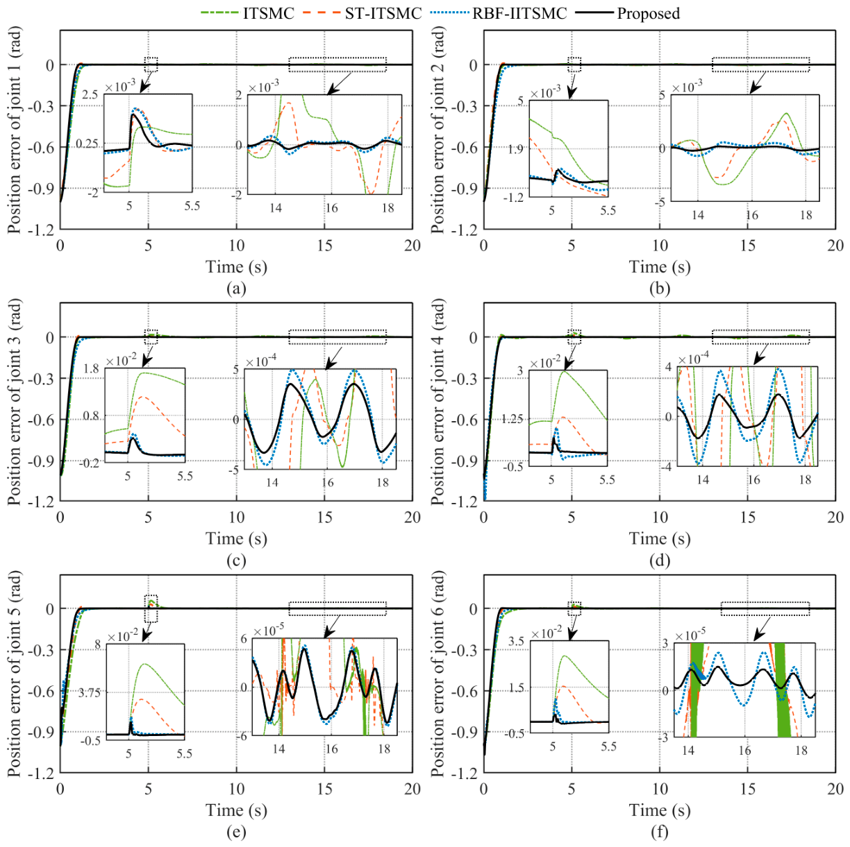
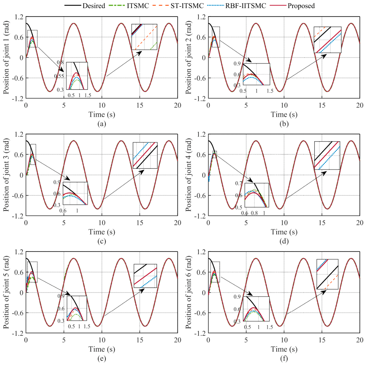
The dynamic tracking capability and steady-state precision of the system are core indicators for evaluating controller performance. Figure 5 and Figure 6 present the trajectory tracking responses and their corresponding error evolution curves of the six joints under the four control schemes, respectively.

It can be observed from the joint position tracking trajectory curves in Figure 5a–f that under the comprehensive operating conditions involving parameter perturbations, complex friction, and external time-varying disturbances, all four control schemes can essentially track the desired sinusoidal trajectories. However, by observing the locally magnified views, it is evident that both the conventional ITSMC and the ST-ITSMC exhibit observable deviations in tracking precision. Further analysis of their transient characteristics reveals that while the conventional ITSMC suffers from sluggish convergence, the ST-ITSMC, leveraging its advanced second-order sliding mode technique, significantly accelerates the transient response. However, inherently relying on conservative high gains to counteract lumped uncertainties and lacking a neural feedforward compensation mechanism, the ST-ITSMC struggles to effectively suppress the unmodeled dynamics and coupling effects of the system, leading to residual tracking deviations. Although the RBF-IITSMC based on empirical parameters improves the tracking performance to a certain extent, its tracking trajectories still fail to perfectly coincide with the desired curves. In contrast, the tracking trajectories of the proposed ASPSO-optimized RBF-IITSMC control strategy achieve the highest degree of coincidence with the desired trajectories.

Figure 6 details the position tracking error evolution curves of specific coupling joints under the four control schemes. From the error curves in Figure 6, it can be clearly observed that the ASPSO-optimized RBF-IITSMC control method possesses significant advantages in terms of convergence speed, error fluctuation amplitude, and overall steady-state precision. In the initial stage of system operation, the tracking error of this method rapidly converges from the initial value of approximately $-1.0 \mathrm{rad}$ into a strict error band of $\pm 2\times {10}^{-4} \mathrm{rad}$, exhibiting minimal overshoot. Subsequently, upon entering the steady-state phase, compared to the conventional ITSMC whose steady-state error generally remains at the magnitude of ${10}^{-3} \mathrm{rad}$, the proposed method significantly reduces it to the order of ${10}^{-4}$ or even ${10}^{-5} \mathrm{rad}$, demonstrating exceptional tracking precision. It is worth noting that at $t=5 \mathrm{s}$, a step impact disturbance is injected into the system joints, wherein Joints 1 to 3 instantaneously bear an abrupt load of $10 \mathrm{N}·\mathrm{m}$. Facing such abrupt and severe operating conditions, both the conventional ITSMC and ST-ITSMC frameworks exhibit substantial error spikes, and the recovery time of the systems is relatively long. In contrast, the proposed method combines real-time RBF neural network compensation with optimal control parameters. This synergistic effect limits the peak variation to less than $1\times {10}^{-4} \mathrm{rad}$. Furthermore, the tracking error rapidly decays and returns to the steady state within approximately $0.5 \mathrm{s}$. This proves that the strategy possesses transient response performance and robust recovery capability when confronting abrupt extreme impacts.

Table 3. Steady-state MAE of the joint position tracking.

Joint	ITSMC	ST-ITSMC	RBF-IITSMC	Proposed Method
Joint 1	1.119 × 10−3	5.595 × 10−4	1.486 × 10−4	7.834 × 10−5
Joint 2	1.215 × 10−3	9.523 × 10−4	3.421 × 10−4	1.173 × 10−4
Joint 3	2.113 × 10−3	8.550 × 10−4	2.484 × 10−4	1.840 × 10−4
Joint 4	2.802 × 10−3	8.209 × 10−4	1.907 × 10−4	8.900 × 10−5
Joint 5	2.552 × 10−4	9.333 × 10−5	2.588 × 10−5	2.365 × 10−5
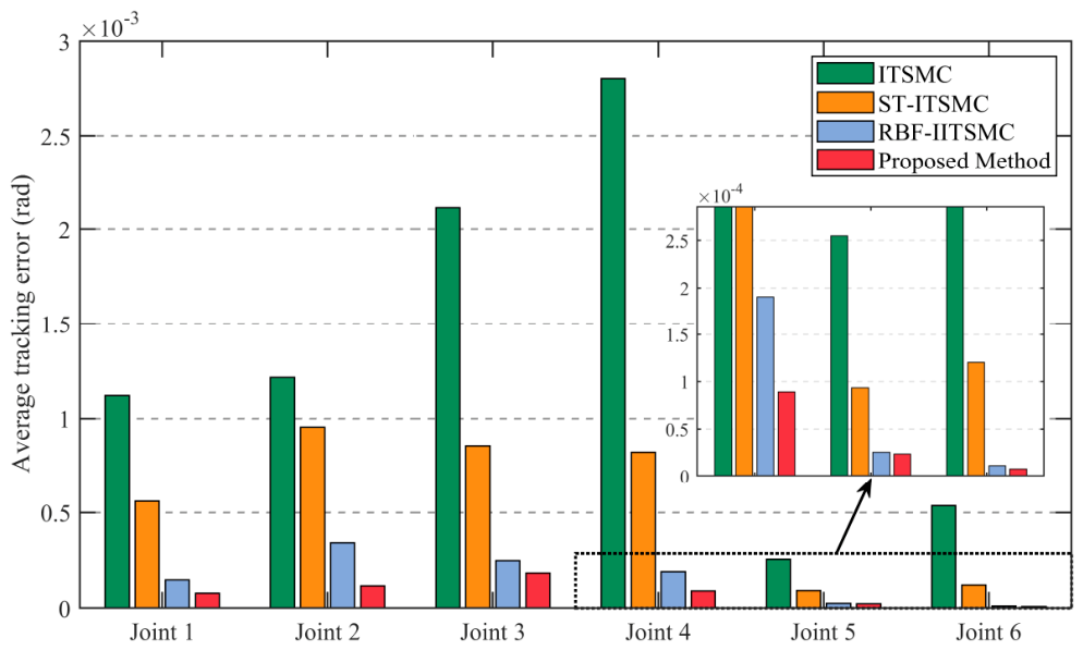
Joint 6	5.350 × 10−4	1.202 × 10−4	1.147 × 10−5	7.937 × 10−6

and Figure 7 quantitatively extract and compare the mean absolute errors (MAE) of each control scheme during the steady-state phase.

Combining Table 3 and Figure 7, it can be intuitively observed that the conventional ITSMC method exhibits the largest steady-state error, generally remaining at the order of ${10}^{-3} \mathrm{rad}$, particularly on Joint 4, which is significantly affected by inertia and gravity loads, where its mean absolute error reaches as high as $2.802\times {10}^{-3} \mathrm{rad}$. Although the ST-ITSMC and RBF-IITSMC gradually reduce the error magnitude, a certain static deviation still exists. In contrast, the mean absolute errors of the proposed ASPSO-optimized RBF-IITSMC method across all joints are strictly confined to extremely low levels, reaching the order of ${10}^{-4}$ to ${10}^{-6} \mathrm{rad}$. For example, on Joint 1, the MAE of the proposed method is only $7.834\times {10}^{-5} \mathrm{rad}$, representing a reduction of approximately $93.0\%$ compared to the conventional ITSMC; on the terminal Joint 6, the error is further reduced to $7.937\times {10}^{-6} \mathrm{rad}$, a reduction of approximately $98.5\%$ compared to the conventional ITSMC. Comparative analysis indicates that the proposed strategy achieves a fast time response and eliminates static tracking errors, even in highly complex disturbance environments. Overall, this approach substantially enhances both the tracking precision and robustness of the robotic arm during complex tasks.

4.2.2. Chattering Suppression and Boundary-Layer Sensitivity Analysis

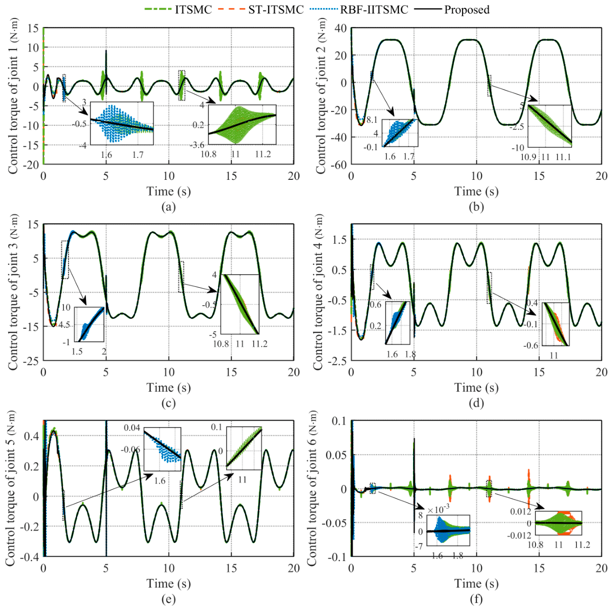
The safe operation of physical actuators is highly dependent on the smoothness of the control torque. Figure 8 comparatively illustrates the control input torque curves of each joint under the four control strategies.

As shown in Figure 8, due to the excessive reliance of the conventional ITSMC algorithm on the high-frequency switching sign function, its output torque exhibits continuous high-frequency chattering phenomena throughout the entire global time domain. From the locally magnified views, it can be intuitively observed that the torque output waveform of the conventional ITSMC is relatively violent, with the envelope bandwidth of its local chattering amplitude reaching $\pm 4 \mathrm{N}·\mathrm{m}$. In contrast, although the ST-ITSMC and the RBF-IITSMC smooth the switching term to prevent continuous global chattering across the time domain, they still exhibit localized torque spikes and high-frequency oscillations during commutation transitions due to the lack of global synergistic parameter optimization. For instance, the locally magnified view of Joint 4 in Figure 8d indicates that during the trajectory commutation phase, the ST-ITSMC generates torque fluctuations, while the RBF-IITSMC exhibits a local chattering amplitude of approximately $0.2 \mathrm{N}·\mathrm{m}$ near $1.7 \mathrm{s}$. Furthermore, in the magnified view of Joint 6 in Figure 8f, the ST-ITSMC produces a local torque spike of approximately $0.03 \mathrm{N}·\mathrm{m}$ around $14.5 \mathrm{s}$, and the RBF-IITSMC yields a local chattering envelope reaching $5\times {10}^{-3} \mathrm{N}·\mathrm{m}$ near $15 \mathrm{s}$. In contrast to this, the proposed ASPSO-optimized RBF-IITSMC composite control strategy exhibits excellent chattering suppression performance. As can be seen from Figure 8, the control torque output by the proposed method exhibits a highly continuous and smooth regular sinusoidal evolution trend, indicating that the controller internally achieves real-time dynamic reverse cancelation of external time-varying nonlinear disturbances. Specifically, the proposed method strictly suppresses the high-frequency chattering amplitude of each coupling joint to below $0.1 \mathrm{N}·\mathrm{m}$, which represents an overall reduction in chattering amplitude of approximately $96.6\%$ compared to the conventional ITSMC. Even when the system is subjected to an abrupt step impact at $t=5 \mathrm{s}$, the controller torque proposed in this paper only generates a slight adjustment at the instant of commutation impact, and then rapidly recovers to a smooth state within $0.15 \mathrm{s}$, suppressing the control saturation or global high-frequency oscillation phenomena common in sliding mode control.

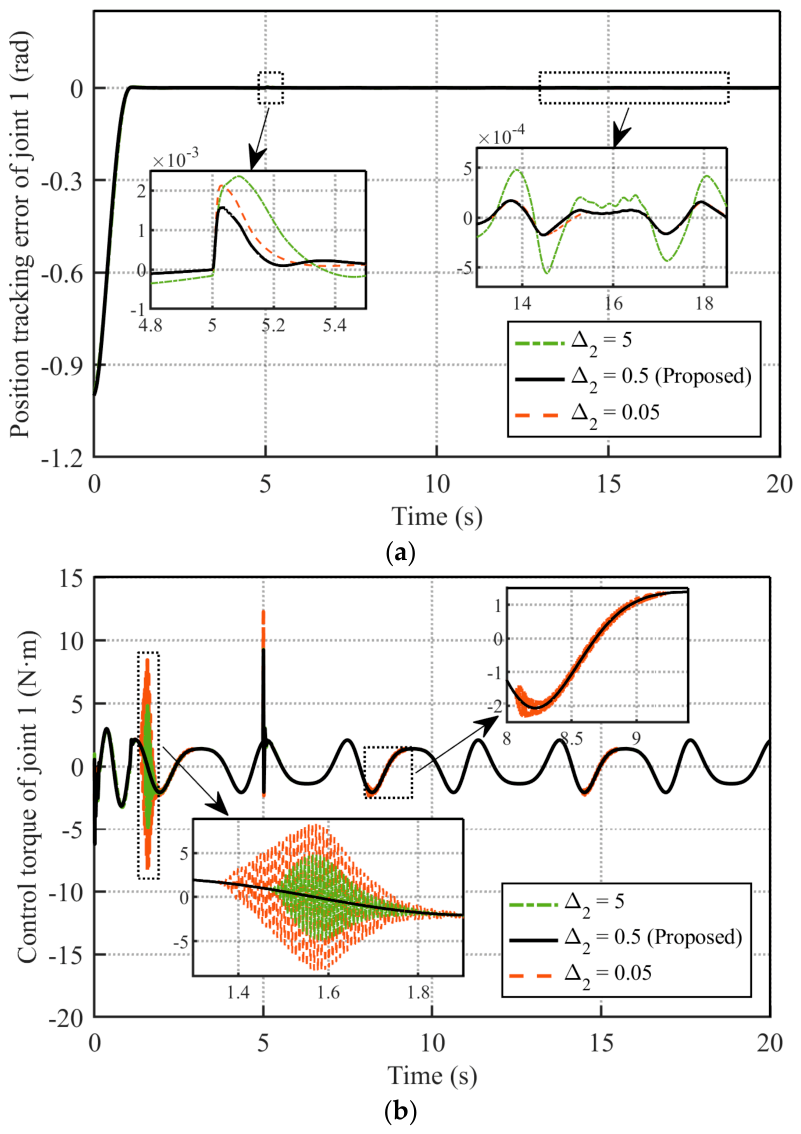
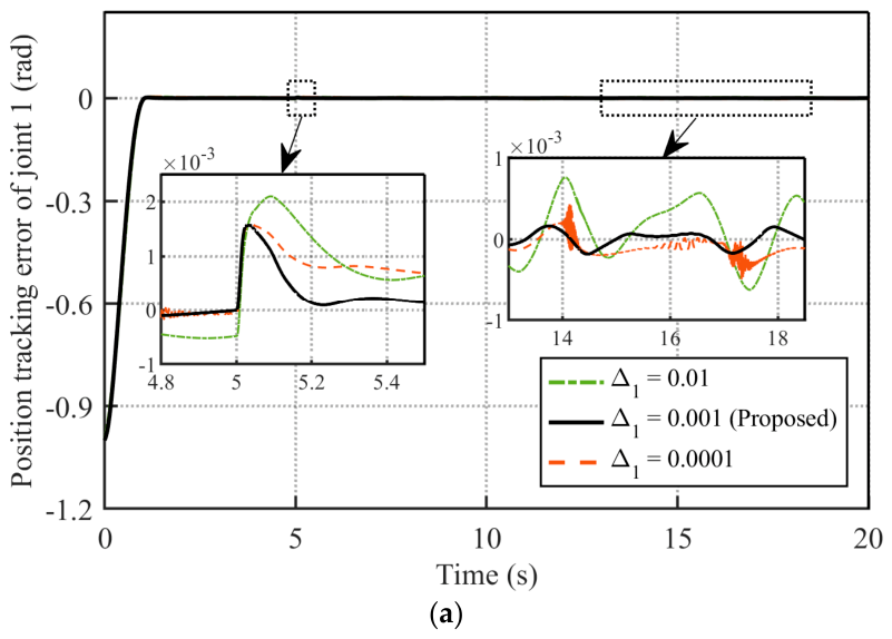
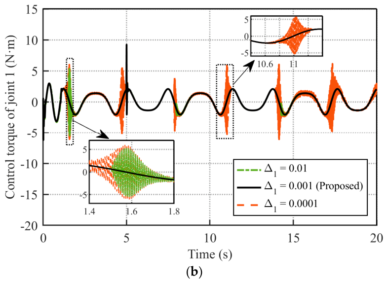
Furthermore, the chattering suppression performance and tracking precision are fundamentally governed by the boundary-layer configurations. To justify the selected parameters ${\Delta }_1$ and ${\Delta }_2$, dynamic sensitivity analysis was conducted by varying these parameters across an order of magnitude. Figure 9 demonstrates the system responses under divergent ${\Delta }_1$ values. Applying a large boundary layer ensures torque smoothness but compromises robustness, resulting in a sluggish transient recovery during the impact disturbance at $t=5 \mathrm{s}$. Conversely, an overly conservative boundary layer approximates the discontinuous signum function, which enhances tracking accuracy but intrinsically triggers high-frequency torque chattering. The proposed value achieves a structural optimum. Correspondingly, Figure 10 illustrates the sensitivity analysis for ${\Delta }_2$. Expanding the boundary deteriorates steady-state precision, whereas aggressively minimizing it induces violent torque chattering spikes during trajectory commutation phases (e.g., near 2 s). These comparative results explicitly validate that the proposed parameters optimally balance the fundamental trade-off between tracking precision and continuous control effort.

4.2.3. Robustness and Tracking Performance Validation Under Multi-Frequency Trajectories

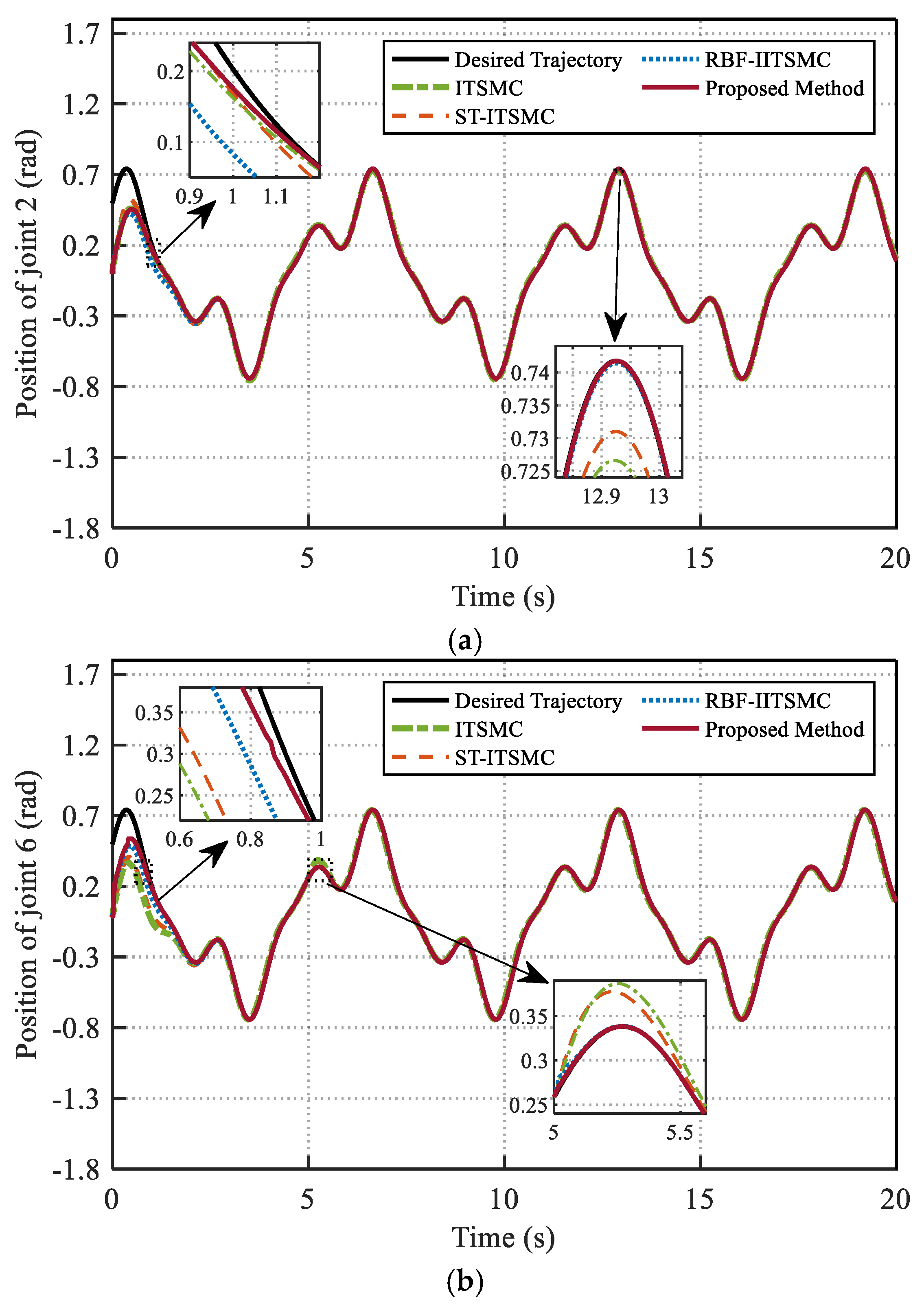
To further validate the comprehensive robustness of the proposed scheme against complex, high-frequency excitations, an aggressive multi-frequency composite trajectory was designed: $q_{di}=0.5\cos \left(t\right)+0.2\sin \left(3t\right)+0.1\sin \left(5t\right)[\mathrm{rad}]$ $(\mathrm{i}=1,\dots ,6)$. Joint 2 (subjected to massive inertial and gravitational loads) and Joint 6 (the low-inertia terminal effector) were selected for specific analysis. To systematically evaluate the controller performance under these conditions, the comparative simulation results are presented across three dimensions: the position tracking trajectories, the position tracking error evolution, and the corresponding control input torques

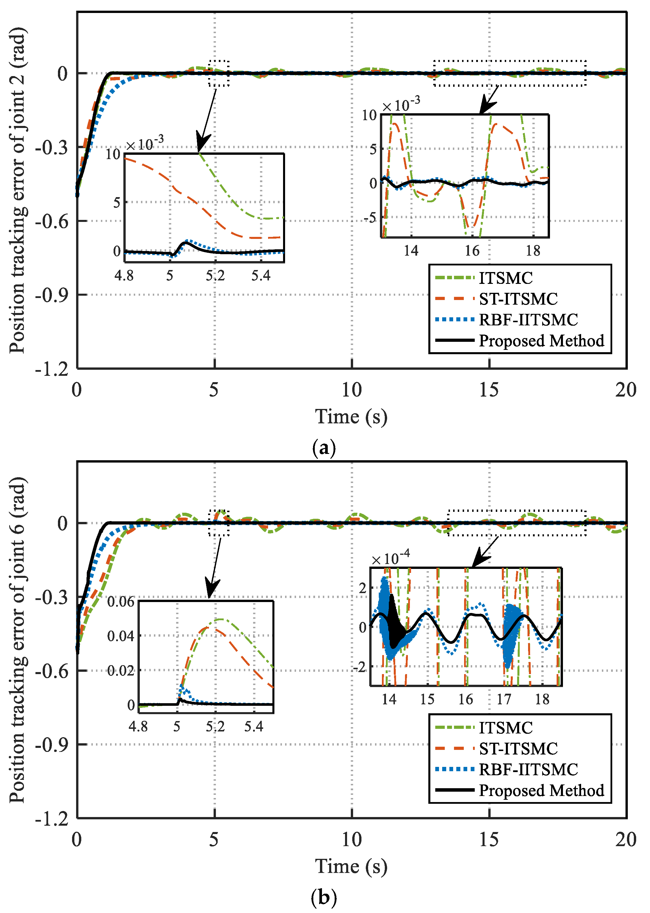
Figure 11 presents the position tracking trajectories. Under the continuous high-frequency direction reversals, the baseline controllers without neural feedforward (i.e., ITSMC and ST-ITSMC) exhibit distinct amplitude attenuation at the trajectory extremums. For instance, the locally magnified views near 12.9 s for Joint 2 and 5.2 s for Joint 6 indicate that the ITSMC and ST-ITSMC fail to reach the desired trajectory peaks, reflecting a constrained dynamic tracking bandwidth. The fixed-parameter RBF-IITSMC mitigates this amplitude attenuation but still exhibits marginal deviations. In contrast, the proposed method strictly coincides with the composite reference trajectory without observable structural delay.

This dynamic tracking superiority is further quantified in the position tracking error evolution curves depicted in Figure 12. During the steady-state tracking phase (e.g., 14 s to 18 s), the ITSMC and ST-ITSMC generate persistent oscillatory static errors due to their inability to fully counteract the time-varying composite disturbances. Furthermore, upon the injection of the step impact at t = 5 s, these two baselines undergo significant transient error spikes (e.g., approaching for Joint 6). While the RBF-IITSMC attenuates the impact spike, its tracking error produces severe high-frequency oscillations in the steady-state region (as explicitly shown in the Joint 6 magnified view), which directly mirrors its internal control torque chattering. The proposed method suppresses these steady-state error oscillations and confines the transient impact deviation to a minimal boundary, achieving a highly rapid transient recovery.

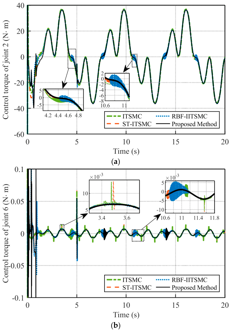
Furthermore, Figure 13 illustrates the control input torques required to satisfy these dynamic specifications. The multi-frequency trajectory intensively excites the unmodeled high-frequency dynamics and amplifies inter-joint coupling effects. As depicted in the magnified views, the ITSMC and ST-ITSMC produce conspicuous local torque spikes during rapid velocity transitions (e.g., near 3.5 s and 11.4 s for Joint 6). Conversely, the fixed-parameter RBF-IITSMC avoids solitary spikes but generates persistent high-frequency chattering (e.g., between 10.6 s and 11 s for Joint 2, and 10.6 s to 11.8 s for Joint 6). This phenomenon indicates that integrating a neural network compensator with manually tuned static parameters leads to structural mismatch under aggressive commutation commands. The proposed ASPSO-optimized method effectively attenuates these phenomena. By penalizing the $J_{\mathrm{Smooth}}$ cost index, the algorithm identifies a synergistic parameter matching, which effectively smooths the control effort and significantly minimizes the chattering amplitude for both the heavy-inertia Joint 2 and the sensitive low-inertia Joint 6. These comparative torque profiles substantiate that the proposed optimization framework structurally maintains a rational balance between tracking agility and control input smoothness.

4.2.4. Comprehensive Evaluation of the ASPSO Framework

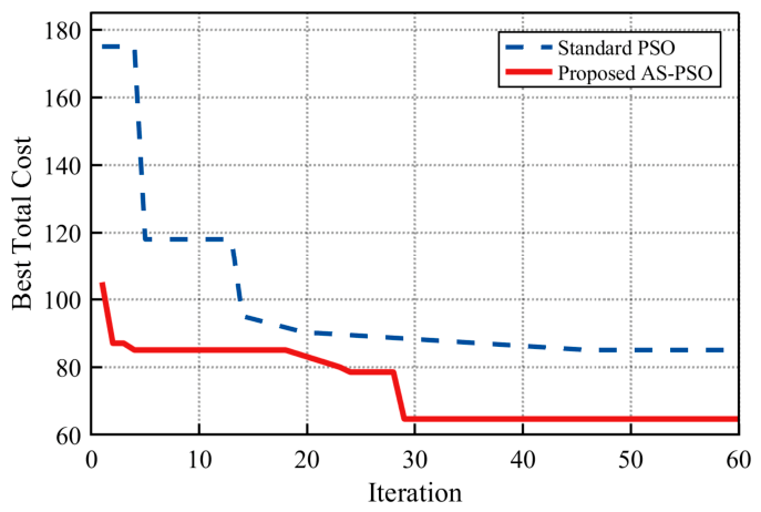
To explore the parameter tuning mechanism underlying the excellent performance of the controller, this section records and evaluates the evolution trajectory of the composite cost function during the parameter optimization process of the adaptive optimization algorithm, as illustrated in Figure 14.

From the convergence curve in Figure 14, it can be seen that in the early stage of iteration (the first 15 generations), the ASPSO algorithm conducts a large-scale global exploration within the 15-dimensional parameter space, and the cost function value drops in a step-like manner. Facing the local optimum trap that is highly prone to occur in high-dimensional nonlinear systems, the standard PSO algorithm falls into stagnation at a cost function value of approximately $85$ due to the premature loss of population diversity. In contrast, the state-aware coefficient adjustment and differential mutation mechanisms mitigate the loss of population diversity and enable the search to resume improvement after the observed stagnation between the 20th and 30th generations. Under the adopted population size, iteration budget, and initialization conditions, ASPSO obtains a best-found cost value of 65.45. Compared with the standard PSO, the proposed ASPSO reduces the final composite cost by approximately 23.0%. These convergence results provide numerical support for the effectiveness of ASPSO in the considered controller-parameter-tuning problem.

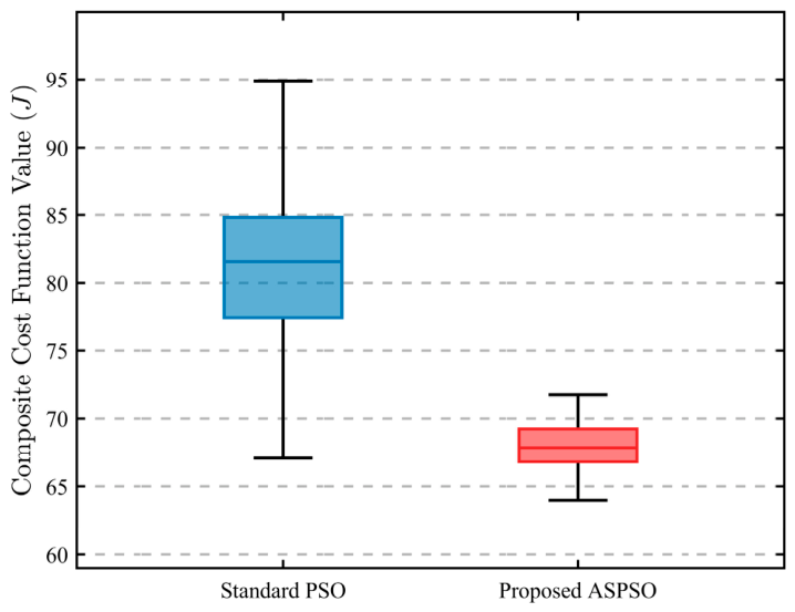
Due to the inherent stochastic nature of swarm intelligence algorithms, evaluating convergence based on a single execution may introduce deterministic artifacts. To rigorously validate the statistical reliability of the proposed framework, a multiple-run analysis was conducted. Both the standard PSO and the proposed ASPSO were independently executed for 30 runs under identical simulation configurations, utilizing randomized initial populations. The statistical distribution of the composite cost function is visualized via the boxplot in Figure 15. It is explicitly observable that the proposed ASPSO not only achieves a significantly lower median cost but also exhibits a remarkably narrower interquartile range, indicating superior robustness against random initializations. To bridge this algorithmic consistency with physical control performance, the comprehensive statistical metrics—including the steady-state tracking MAE of Joint 1—are detailed in

Table 4. Statistical metrics of algorithmic cost and physical tracking performance over 30 independent runs.

Algorithm	Cost Best	Cost Worst	Cost Mean	Cost Std. Dev	Tracking MAE Mean (Joint 1)	Tracking MAE Std. Dev
Standard PSO	68.45	97.34	82.15	7.12	1.04 × 10−4	1.85 × 10−5
Proposed ASPSO	65.23	71.05	68.12	1.45	7.95 × 10−5	0.48 × 10−5

. The analysis demonstrates that the standard PSO suffers from premature convergence, yielding a high standard deviation of 7.12. In contrast, the ASPSO algorithm actively preserves population diversity, drastically reducing the cost standard deviation to merely 1.45. More importantly, the ASPSO-optimized controller consistently achieves a statistical mean tracking MAE of 7.95 × 10⁻⁵ rad, accompanied by an extremely marginal standard deviation of 0.48 × 10⁻⁵ rad. These comparative results solidly substantiate that the high-precision control performance generated by the proposed scheme possesses statistical reliability and consistency.

Furthermore, to evaluate the sensitivity of the optimization results to the selection of the cost-function weights, a sensitivity analysis of the cost-function weights was conducted. We perturbed the baseline values of the primary tracking precision weight ($w_1$) and the torque smoothness weight ($w_2$) by $\pm 20\%$. The ASPSO optimization process was re-executed under these varied conditions. To clearly illustrate the trade-off between tracking accuracy and control effort, both the steady-state Mean Absolute Error (MAE) and the maximum torque chattering amplitude of Joint 1 are recorded in

Table 5. Sensitivity analysis of optimization weights on MAE and torque chattering (Joint 1).

Weight Variations	${\mathit{w}}_1$ Value	${\mathit{w}}_2$ Value	Optimized MAE (rad)	Max Torque Chattering ($\mathbf{N}·\mathbf{m}$)
Baseline	3000	0.020	7.834 × 10−5	0.092
$w_1$ + $20\%$	3600	0.020	7.512 × 10−5	0.098
$w_1$ − $20\%$	2400	0.020	8.201 × 10−5	0.088
$w_2$ + $20\%$	3000	0.024	8.095 × 10−5	0.081
$w_2$ − $20\%$	3000	0.016	7.720 × 10−5	0.105

.

As observed in Table 5, the optimization results strictly follow the expected physical trade-off: increasing the $w_1$ slightly reduces the MAE at the cost of marginally higher torque chattering, whereas increasing the $w_2$ further suppresses torque fluctuations but yields a slightly larger tracking error. Crucially, despite a substantial $20\%$ variation in the predefined penalty weights, the steady-state tracking error fluctuates by less than $5\%$, and the torque chattering remains confined to a safe margin (around 0.1 $\mathrm{N}·\mathrm{m}$). This sensitivity analysis demonstrates that the superior performance of the ASPSO-optimized scheme does not critically rely on strictly fine-tuned initial hyperparameters, validating its algorithmic robustness and practical applicability.

5. Conclusions

This study developed an ASPSO-optimized RBF-IITSMC scheme for trajectory tracking of a 6-DOF robotic arm under lumped uncertainties. The boundary-layer terminal mapping was analytically characterized in terms of its global Lipschitz property, approximation-error bound, and explicit design interval. In addition, the reduced-order RBF formulation separates the uncertainty component approximable from the sliding dynamics from the bounded residual, while ASPSO is employed for the joint tuning of the coupled controller parameters.

The numerical evaluation was conducted in MATLAB/Simulink under the specified conditions, including 20% model-parameter perturbations, nonlinear friction, continuous time-varying disturbances, and abrupt step impacts. Under these tested scenarios, the proposed controller achieved steady-state joint-position MAEs ranging from $7.937\times {10}^{-6}$ to $1.840\times {10}^{-4} \mathrm{rad}$, and the tracking error returned to its steady-state range within approximately 0.5 s after the step impact. For the considered parameter-tuning problem, ASPSO reduced the final composite cost by approximately 23.0% relative to the evaluated standard PSO implementation. The 30 independent runs further showed lower mean cost and smaller variability than standard PSO. These results indicate improved tracking performance and numerical consistency under the adopted simulation and computational conditions.

The findings support the numerical robustness and effectiveness of the proposed method under the considered simulation scenarios and provide a basis for subsequent experimental implementation. Nevertheless, the current evaluation is limited to the simulation environment. The effects of actuator saturation, sensor noise, communication delays, discretization and sampling, and mechanical flexibility have not yet been systematically evaluated. Future work will therefore focus on hardware implementation and experimental assessment under these practical physical and implementation conditions.