Article

On Optimality and Robustness in Linear Dynamic System Identification

by
Marko Živković
1,2,
Zoran Banjac
1,*,
Miloš Pavlović
1,
Tomislav Unkašević
1 and
Branko Kovačević
3
1
Vlatacom Institute, 11070 Belgrade, Serbia
2
Faculty of Technical Sciences, Singidunum University, 11000 Belgrade, Serbia
3
Faculty of Electrical Engineering, University of Belgrade, 11000 Belgrade, Serbia
*
Author to whom correspondence should be addressed.
Mathematics 2026, 14(14), 2663; https://doi.org/10.3390/math14142663
Submission received: 22 June 2026 / Revised: 17 July 2026 / Accepted: 20 July 2026 / Published: 22 July 2026
(This article belongs to the Special Issue Mathematical Modelling and Applied Statistics)

Highlights

What are the main findings?
  • Introduces a novel robust, approximate Newton–Raphson recursive method for linear dynamic system identification.
  • Successfully handles heavy-tailed, non-Gaussian noise using Huber’s robust M-estimation.
  • Rigorously proves strong consistency and asymptotic normality using martingale theory.
What are the implications of the main findings?
  • Huber’s M-estimation prevents parameter tracking failures caused by heavy-tailed noise and outliers.
  • Martingale theory proves that the estimates converge to true values, ensuring longterm system stability.
  • Reaching the Cramér–Rao bound establishes a mathematically verified optimal performance benchmark.

Abstract

Strong consistency and asymptotic error distribution for a new class of nonlinear recursive parameter estimation algorithms of an approximate Newton–Raphson type are established. The system model is given in the discrete-time domain by a linear difference equation with constant parameters. The parameter estimator design is based on martingale theory and the Cramér–Rao (CR) theorem, providing a maximum likelihood (ML)-type optimal recursive parameter identification algorithm, whose minimum asymptotic estimation error covariance matrix achieves the CR bound under the worst-case pdf within a specified class; this worst-case pdf simultaneously yields the maximum asymptotic error covariance matrix within the class. However, the worst-case pdf does not generally exist, making the min–max optimal design indeterminable. Therefore, an approximate ML (AML)-type optimal on a class design, based on a suboptimal worst-case pdf, minimizing the scalar Fisher information within the specified class, has also been developed. The proposed design minimizes the conditional estimation error covariance under the specified suboptimal worst-case pdf. Such an approach results in Huber’s M-robustified version of the AML-based optimal design on the class of contaminated Gaussian pdfs. The practical performance of the proposed approach is analyzed through statistical validation, based on the relative asymptotic estimation efficiency measure and Monte Carlo simulations.

1. Introduction

Modeling is an important activity in various engineering and scientific fields, involving different types of applications, some of which are technical (mechanical, chemical, electrical and hydraulic plants), while others involve biological, medical, ecological, economic and psychological processes, etc. [1,2,3,4,5,6,7,8]. In general, there exist two types of modeling approaches. The first one assumes enough knowledge about the physical phenomenology of the process to incorporate a few idealized physical laws to which the process dynamics is confined, combined with an adequate representation of the noisy measurements. Since a such model is based on a lumped physical phenomenology characterized by the state-space structure, it is called a white-box or state-space model [6,7,8,9,10]. The second one assumes that adequate information about the process to be handled is not available, leading to the need to derive its model solely from input–output data. Since this model is based on a parametric, or polynomial, input–output structure and reflects the absence of process knowledge, it is called a black-box or parametric polynomial input–output model [11,12,13,14,15,16,17]. In this sense, one has to define an experiment to obtain information about the process in question. Furthermore, the design of the experiment must be followed by a step for parameter identification. In general, input–output representations can be used easily for process analysis, simulations and control purposes, while state-space representations may be generalized easily.
Parametric estimation methods have become a cornerstone of modern signal processing [6], with applications ranging from speech processing [18,19,20] and adaptive filtering [21,22,23] to time-series analysis, parameter and state estimation, pattern classification and control [6,7,8,9,10,11,12,13,14,15,16,17]. The works of Ljung, Goodwin, Tsypkin and others provide both theoretical and practical frameworks for the design and performance evaluation of such methods [11,12,13,14,15,24,25]. Parametric methods may be viewed as model-based procedures in which, once the model set is selected, the unknown parameters are estimated from measurement data according to an adopted optimization criterion. When the signal statistics are not exactly known, adaptive techniques based on numerical optimization theory [26,27,28,29,30,31] offer a solution: for stationary signals, the adaptive estimates converge to the optimal ones [6,7,8,11,12,13,14,15,16,17]. The main problem is then the choice of an adaptation algorithm—gradient, Newton–Raphson, etc.—that iteratively adjusts the required parameters (statistics, gains, coefficients) under incomplete prior knowledge. In this context, the quadratic score is optimal in the MMSE sense under Gaussian disturbances, leading to the standard least squares (LS) identification algorithms [2,3,4,5,6,7,8,11,12,13,14,15,16,17]. However, the ML optimal estimation algorithms, as well as adaptive techniques, which rely on the assumption of Gaussian disturbances, are particularly inefficient when dealing with heavy-tailed, approximately Gaussian-distributed observations, which can lead to rare but huge outliers. In this sense, owing to incomplete measurements and communication errors, most industrial and scientific data are contaminated Gaussian-distributed, producing observation and innovation outliers. In addition, structural outliers may occur due to inadequate mathematical models or computational errors [32,33,34,35]. Consequently, investigations have focused on developing robust parameter estimators that effectively suppress the influence of multiple outliers in practice. In robust statistics, such a feature of the estimator is known as resistance robustness. Moreover, owing to the central limit theorem of statistics, it is also desirable that the robust estimator exhibit good performance under both purely Gaussian and heavy-tailed Gaussian measurements, resulting in the efficiency robustness feature. Practical robustness involves both the efficiency and resistance features, making it appealing to engineers and practitioners [32,33,34,35]. Huber’s approximate ML (AML), or M-robust, concept is frequently used to design practically robust parameter estimates in various applications [32,33,34,35,36,37,38,39].
The other two robustness concepts, namely min–max and qualitative robustness, are based on rigorous mathematical approaches and are thus more appealing to scientists and theoretical workers. In this sense, qualitative robustness involves the definition of Hampel’s influence function as an efficient tool that enables a robust estimator to effectively eliminate the influence of multiple outliers [39]. In addition, Huber’s min–max robust statistical approach minimizes the maximum anticipated asymptotic estimation error attained at the least favorable, or worst-case, distribution within the specified class [35]. This, in turn, provides the maximum asymptotic rate of the estimates’ convergence under the worst-case observation noise distribution. However, the matrix optimization problem is a nonclassical variational task, so its solution does not generally exist [26,27,28]. In particular, for static regression plants or linear finite impulse response (FIR) dynamic systems, the worst-case pdf is derived from the minimization of the scalar Fisher information within the specified class [15,35,38]. In addition, most robust estimation schemes are minimization procedures, which leads to highly nonlinear parameter estimation algorithms [32,33,34,35,36,37,38,39]. Furthermore, based on the computational requirements of online or real-time applications, one can choose to calculate the estimate recursively rather than nonrecursively in a batch processing mode [1,2,3,4,5,6,7,8,11,12,13,14,15,16,17].
In relation to the existing literature, the proposed approach differs from closely related methods in the following aspects. Classical recursive ML and prediction-error identification schemes [11,12,13,14,15,16,17] rely on the quadratic score, optimal under Gaussian disturbances, and their robust modifications are typically introduced heuristically, without an explicit optimality framework. Huber’s M-robust estimation theory [35,39], as well as the min–max optimal identification of Poljak and Tsypkin [15,24,25], provides such a framework, but the exact worst-case solution is available only for static regression and FIR structures. Robust recursive Newton-type algorithms, e.g., [21,22,23,24,25,38], address the ARX/IIR case, but complete asymptotic characterization is lacking. The contributions of this paper are therefore threefold: (i) the strong consistency and asymptotic normality of a class of approximate Newton–Raphson recursive estimators with a general admissible influence function are rigorously established by martingale theory (Theorems 1 and 2); (ii) it is shown that the exact min–max optimal design is generally indeterminable for IIR dynamic systems, which motivates the proposed AML-based optimal design on a class, minimizing at each stage the conditional estimation error covariance under a suboptimal worst-case pdf that minimizes the scalar Fisher information; (iii) the link between the optimal nonlinearity and the gain matrix recursion is established through the statistical linearization coefficient, for which two realizable approximations (fixed and variable factors) are proposed and comparatively analyzed.
In this paper, a new class of nonlinear recursive estimation algorithms of an approximate Newton–Raphson type for the parameter identification of linear discrete time-invariant dynamic stochastic systems is considered. The manuscript is organized in the following manner. The introductory Section 1 presents a brief discussion of frequently used approaches to dynamic system modeling, involving system parameter identification and robust estimation concepts. Section 2 is devoted to designing a class of approximate Newton–Raphson-type recursive parameter estimation algorithms under the exactly known observation noise statistics. Conditions under which the derived identification algorithm converges with probability one (w.p.1), or almost surely (a.s), are discussed in Section 3. In addition, the asymptotic estimation error analysis, involving the convergence of the asymptotic estimation error to a zero-mean Gaussian pdf, is presented in Section 4. The problem of designing a feasible recursive nonlinear M-robustified version of the AML-based optimal parameter estimation algorithm on a class of pdfs is considered in Section 5. Section 6 contains the implementation considerations and the statistical linearization analysis, based on the relative estimation efficiency quantitative measure. The performance analysis is carried out for the practically important class of Gaussian-distributed observations corrupted by impulsive noise or outliers. Section 7 presents Monte Carlo simulation results that illustrate the theoretical analysis from Section 6, as well as investigating the ability of the proposed parameter identification procedure to achieve practical robustness, involving both the resistance and efficiency robustness characteristics. Concluding remarks are presented in Section 8. The detailed derivation of the asymptotic estimation error zero-mean normal distribution, using the martingale theory results, is presented in Appendix A.

2. Problem Formulation

An abstract single-input single-output (SISO) linear discrete time-invariant dynamic stochastic system is described by a linear difference equation with constant parameters:
y i = k = 1 n a k * y i k + k = 1 m b k * u i k + e i
Here, y i is the output signal sample, u i is the input signal sample, and e i is the random disturbance, or observation noise, sample at the discrete time indexed by i . In normal operation, the observed input–output sequences u i and y i are wide-sense stationary random discrete-time processes [9,10,11,12,13,14,15,16,17]. The random noise samples e i are zero-mean, independent and identically distributed (i.i.d.) scalar real random variables. Introducing the shift operator q k x i = x i k , one can rewrite (1) in the form
A q 1 y i = B q 1 u i + e i .
where the characteristic polynomial A and control polynomial B are given by
A q 1 = 1 + k = 1 n a k q k ; B q 1 = k = 1 m b k q k
assuming that the polynomial orders m and n are given in advance. In addition, relation (1) can also be rewritten in the linear regression form
y i = θ * T Z i + e i ; θ * T = a 1 * , , a n * , b 1 * , , b m *
where θ * is the true n + m × 1 column vector of unknown system parameters to be estimated, while Z i is the information, or regression, n + m × 1 column vector
Z T i = y i 1 , , y i n , u i 1 , , u i m
Since the disturbance or noise sequence e i directly enters relation (2), this representation belongs to the family of equation errors (EEs), in which the EE is represented by a white real scalar discrete stochastic process [14]. Representation (2) is also called an autoregressive with exogenous input (ARX) model [5,6,7,8,9,11,12,13,14,15,16,17]. In addition, model (2) is characterized by an infinite impulse response (IIR) under the unit δ -impulse excitation. In particular, if the polynomial A = 1 in (3), then representation (2) is known as a finite impulse response (FIR) model [2,3,4,5,6,7,8,11,12,13,14,15,16,17].
The problem of the recursive identification of the system described by (4) is considered as the task of estimating in real time the unknown parameter vector θ * by utilizing the current input–output observations u i , y i . The formulation of the identification problem reduces to the choice of prediction model y ^ i | θ , where θ T = a 1 , , a n , b 1 , , b m is the given vector of model parameters, as well the choice of an identification performance criterion, or quality measure, to be minimized,
J θ = E F ε i , θ ;   ε i , θ = y i y ^ i | θ
where E is the mathematical expectation. Here, ε is the prediction error, also known as the measurement residual or innovation. Moreover, F : R R is assumed to belong to the class F of admissible score functions, where F F if F is real-valued, symmetric, F z = F z , convex, F 0 = 0 , and absolutely continuous with derivative ψ z = F z existing for almost all z R [5,6,7,8,11,12,13,14,15,16,17,21,22,23,24,25]. The solution of the posed optimization problem in (6) reduces to choosing an online parameter identification algorithm
θ ^ i = f θ ^ i 1 , u i , y i
which recursively calculates the current vector estimate θ ^ i of the unknown parameter vector θ * in (4) from the preceding parameter vector estimate θ ^ i 1 and the current input–output observations u i , y i . Therefore, the aim is to determine optimally, in some sense, the prediction model y ^ | and the score function F in (6), as well as the estimation procedure f in (7). Here, prior information about the system defines an optimal prediction model in the MMSE sense. Thus, taking into account (2)–(5), and utilizing MMSE criterion E ε 2 i , θ , one gets the prediction model [5,6,7,8,11,12,13,14,15,16,17]
y ^ i | θ = 1 A q 1 y i + B q 1 u i = θ T Z i
Let the i.i.d. disturbances e i in (2) admit a probability density function p : R R + , R   p z d z = 1 , which is assumed to be symmetric, i.e., p z = p z , strictly positive and absolutely continuous on R , with finite Fisher information I p = p / p 2 p d z < [9,10]. Under these conditions, the ML-based optimal score function and the associated influence function are well defined and given by [5,6,7,8,9,10,11,12,13,14,15,16,17,18]
F z = F 0 z = log p z ;   ψ z = ψ 0 z = d F 0 z d z = F 0 z
To derive the optimal recursive identification algorithm f in (7), let us also consider the empirical average loss
J i θ = i 1 k = 1 i F ε k , θ
Under certain, mild conditions, the empirical criterion J i θ in (10) asymptotically converges to the optimal criterion J θ in (6) [15,24,25]. The empirical criterion in (10) can be minimized recursively using an approximate Newton–Raphson-based iterative numerical algorithm:
θ ^ i = θ ^ i 1 i θ 2 J i θ ^ i 1 1 i θ J i θ ^ i 1 ;   θ ^ 0 = θ 0
where θ = / θ = / a 1 , , / b m T is the gradient vector, or the partial derivative operator [15,24,25,31]. Moreover, for a large enough time index i , the optimality condition implies that the gradient vector is close to zero, i.e., θ J i 1 θ 0 , and one obtains
i θ J i θ ^ i 1 = Z i ψ ε i , θ ^ i 1 ;           ψ = F i θ 2 J i θ ^ i 1 = α k = 1 i Z k Z T k ;             α = E p ψ e
with E p being the expectation with respect to the pdf p of the i.i.d. random variable e i in (2). In addition, let us introduce the current gain matrix in the i -th discrete-time stage:
Γ i = i θ 2 J i θ ^ i 1 1 = α k = 1 i 1 Z k Z T k + α Z i Z T i 1 = Γ i 1 + α Z i Z T i 1
Taking into account the matrix inversion lemma, one gets, from (11) and (12), the parameter identification algorithm
θ ^ i = θ ^ i 1 + Γ i Z i ψ ε i , θ ^ i 1 ;   θ ^ 0 = 0
ε i , θ ^ i 1 = y i Z T i θ ^ i 1 ;   α = E p ψ e
Γ i = Γ i 1 Γ i 1 Z i Z T i Γ i 1 α 1 + Z T i Γ i 1 Z i ;   Γ 0 = γ I
where I is an identity matrix and γ is a finite positive constant, while α is the statistical linearization coefficient in (12). In general, prior information about the true parameter vector θ * in (4) defines the initial values of the parameter estimates θ ^ 0 and the gain matrix Γ 0 [11,12,13,14,15,16,17,23,24,25]. If such reliable prior information does not exist, the most frequently used initial guesses are those given in relations (14) and (16), namely θ ^ 0 = 0 and Γ 0 = γ I , respectively.
A special case of the recursive nonlinear algorithm (14)–(16) is the recursive linear least squares (RLS) method, which is optimal, in the MMSE sense, for the Gaussian disturbance pdf p . It is widely recognized that, under specific conditions regarding the random disturbances e i in (4), the RLS parameter estimates are consistent [5,6,7,8,11,12,13,14,15,16,17,40,41]. In this context, the asymptotic performance of the nonlinear parameter estimation algorithm (14)–(16) involving a.s or w.p.1 convergence, as well as the convergence of the asymptotic estimation error to a zero-mean normal pdf, is analyzed in the following.

3. Brief Review of Parameter Estimate Consistency

In general, the convergence of recursive stochastic estimation procedures may be analyzed using at least two approaches. The first one is the ordinary differential equation (ODE) approach, based on defining the deterministic ODE associated with the parameter estimation algorithm under consideration, together with the application of the Lyapunov direct method to analyze the ODE stability [11,12,23,38,42]. The second one is based on standard martingale theory [43,44,45]. In this sense, let Ω , F , P be a probability space, with F 1 F 2 being an increasing sequence of sub- σ -fields F , and let x t be a sequence of real scalar random variables attached to F t [9,10]. Then, the pair x t , F t represents a martingale if the expectation E x t < and the conditional expectation E x t | F t 1 = x t 1 w.p.1. Furthermore, provided that E x t | F t 1 x t 1 w.p.1, the pair x t , F t represents a supermartingale [43,44].
In general, the convergence analysis of the recursive stochastic estimation procedure (14)–(16) can be based on the assumptions concerning the disturbance or noise sequence e i in (4); the features of the nonlinear transformation or influence function ψ in (14) applied to the prediction error, innovation or measurement residual ε in (15); and the properties of the gain matrix sequence Γ i in (16). A possible set of assumptions that ensures the strong consistency of the parameter estimate sequence θ ^ i in (14) is summarized in Theorem 1 below.
Theorem 1. 
Let model (4) and the algorithm in (14)–(16) satisfy the following conditions:
C1. 
The stochastic sequence  e i  consists of i.i.d. real scalar random variables, having a symmetric pdf  p  with zero mean  E p e i = 0  and finite variance  E p e 2 i = σ e 2 < .
C2. 
The odd real scalar influence function  ψ  is continuous almost everywhere.
C3. 
The function  ψ  is bounded, satisfying  ψ z k 1 1 + k 2 z  ,  0 < k 1 <  ,  0 k 2 < .
C4. 
The linearization coefficient  α  in (12) is a positive and finite constant;  0 < α k 3 < .
C5. 
There exists a real positive constant  δ 1 > 0  such that
z ϕ z 1 2 δ 1 α z 2 ;   ϕ z = E ψ z e i | F i 1
with  F i  being the sequence of increasing sub- σ -fields, generated by the observations up to present discrete-time  i  , while the coefficient  α  is defined by condition C4.
C6. 
If the scalar term  r i = T r Γ 1 i  , where  T r  denotes the matrix trace, then the observation vector  Z i  in (5) satisfies
Z i 2 M log δ 2 r i ;   δ 2 > 0 ,   M 0
with   being the Euclidean norm.
C7. 
There exists a real constant  c > 1  , such that
lim i log c r i / λ min Γ 1 i = 0     w . p . 1 and   lim i λ min Γ 1 i =         w . p . 1
where  λ min  is the minimum eigenvalue of a matrix.
Then, the parameter estimate sequence  θ ^ i  exhibits strong consistency
lim i θ ^ i = θ *   w . p . 1 , o r   P lim i θ ^ i = θ * = 1
where  P  denotes the probability of a random event.
The proof of Theorem 1, based on the standard martingale theory results, is presented in [41]. In this context, Neveu’s lemma is the basic martingale convergence result [43].
It is worth noting that the polynomial A in (2) can be arbitrary, so that the algorithm in (14)–(16) can also be used for the parameter estimation of unstable systems. However, since bounded input–bounded output (BIBO) stability is one of the most desirable properties of a linear discrete time-invariant dynamic system, it is supposed here that the polynomial A in (2) is a stable one [6,7,8,9,10,11,12,13,14,15,16,17]. Moreover, hypothesis C1 represents a standard whiteness condition on random disturbances or observation noise [9,10]. In other words, assumption C1 results in a zero-mean white observation noise sequence e i in (4) with finite variance σ 2 . Conditions C2–C5 define a class of admissible nonlinear residual transformations ψ in (14) of the prediction residuals ε in (15). In particular, for the linear residual transformation ψ , condition C5 reduces to δ 2 < 2 . Furthermore, it is commonly adopted that k 2 = 0 in C3, yielding a ψ -function bounded by a finite constant. Moreover, under such a bounded ψ -function, the noise variance σ 2 in C1 need not be finite. In addition, condition C5 is fulfilled if the function
ϕ a = 0 ψ z + a ψ z a d P z
is monotonically nondecreasing [15,23,24,25,38]. Taking into account hypotheses C1 and C2, the last requirement is satisfied if the nonlinear residual transformation ψ and the observation noise probability distribution function P have a common point of increase, meaning that
ψ z + ε > ψ z ε ,   P z + ε > ψ z ε
for some real scalar z -value and every real scalar value ε > 0 . This, in turn, results in a ϕ a > 0 for a 0 and ϕ 0 = 0 . Therefore, hypothesis C5 is fulfilled if the odd and almost everywhere continuous ψ -function is monotonically nondecreasing and piecewise continuously differentiable. As mentioned above, a desirable requirement is the boundedness of the ψ -function, with k 2 = 0 in C3. Additionally, even though the polynomial A in (2) is stable, the underlying stochastic system may have signals that are unbounded [6,7,8,9,10,11,12,13,14,15,16,17]. Hence, hypothesis C6 defines the growth of the observation vector Z i in (5), with M being an arbitrary positive real constant. In particular, the case δ 2 0 (i.e., Z i 2 M ) corresponds to bounded measurement data. Finally, some assumptions on the input data must be imposed to obtain fairly good identification results. Such an input requirement is called the persistent excitation condition [5,6,7,8,11,12,13,14,15,16,17]. In this sense, C7 is a rather weak hypothesis for consistent parameter estimates [40,41]. Taken together, both conditions C6 and C7 ensure that the gain matrix Γ i in (16) approaches zero at the proper rate when the time index i increases, i.e., neither too fast nor too slow. In other words, the aim of such an assumption is to ensure that the observations contain sufficient information about the unknown parameter vector θ * in (4). This requirement is physically similar to the concept of stochastic observability, describing the information content of measurement data [9,11,12,13,14,15,16,17].
It is worth emphasizing that not all of conditions C1–C7 carry the same practical weight. Conditions C1 and C3 are mild and easily arranged by design, since they concern the whiteness of the disturbance sequence and the boundedness of the influence function, respectively, both of which are properties of the estimator rather than of the observed data. Conditions C6 and C7, by contrast, concern the growth rate of the observation vector and the persistent excitation of the input and are therefore more likely to be only approximately satisfied over a finite data record in a practical application. However, since C6 and C7 are asymptotic requirements, a transient violation over a limited number of samples does not by itself invalidate the use of the algorithm; it may, at most, slow down the empirical rate of convergence until the observations again contain sufficient information about the parameter vector to be estimated.
In general, in addition to the asymptotic convergence analysis of the recursive nonlinear algorithm (14)–(16), an estimation algorithm must provide a suitable measure of the estimation quality. In this sense, the asymptotic estimation error distribution is analyzed in the following.

4. Asymptotic Estimation Error Distribution

Once the convergence properties of the parameter estimates, (14)–(16), are established, the next natural question is to determine how rapidly the estimates converge to the limit. In particular, if the asymptotic pdf of the estimation error is a zero-mean normal, the mean value and covariance matrix represent the sufficient statistics [9,10]. Thus, one should analyze the convergence rate, as well as the estimator optimality, by utilizing the asymptotic covariance matrix of the estimation error. In this context, the asymptotic estimation error analysis results are presented in the following Theorem 2. Therefore, let us first state a few auxiliary lemmas, which are used in the asymptotic estimation error analysis, together with the standard martingale convergence results [43,44].
Lemma 1 
(Ljung and Söderström) [11]. Let  b n  be a sequence of scalar real quantities such that  b n > 0 ,  lim n b n = 0  and  n b n < c k = 1 n 1 b k 2 + n α 1  for some real constant  c > 0  and  α 1 0 , 1  . Then,
k = 1 n 1 b k 2 < c n β ;   β = max 0 , 2 α 1 1 for     α 1 1 / 2 ε ,     ε > 0 for     α 1 = 1 / 2
Lemma 2 
(Hall and Heyde) [44]. Let  x t  be a scalar real discrete stochastic process, and let the sequence  L n = t = 1 n x t  converge w.p.1 to  L , with the difference  V n = L L n = t = n + 1 x t  providing  V n 2 = t = n + 1 E x 2 t | F t 1 , and  S n 2 = E V n 2 . Let us assume further that the following hypotheses are satisfied:
(I)
The probability  P V n 2 S n 2 > ε < δ , for some  ε > 0 .
(II)
lim n 1 S n 2 t = n + 1 E x 2 t I x t ε S n = 0 , for all  ε > 0 , where  I  is the indicator function. Then,
V n S n = L L n S n     D     N 0 , 1
where the symbol  D  denotes the convergence in distribution, while  N 0 , 1  is the standard normal pdf with zero-mean and unit variance.
Lemma 3 
(Kronecker’s lemma) [45]. Let the sequence  i = 1 n x i  of real numbers  x i  converge, and let  b n  be a monotonically increasing sequence of positive real numbers satisfying  lim n b n =  . Then,
lim n 1 b n k = 1 n b k x k = 0
Lemma 4 
(Neveu’s martingale convergence lemma) [43]. Let  z i  be a sequence of non-negative real scalar random variables, while  F i  is a sequence of increasing sub-  σ  -fields, defined on the probability space  Ω , F , P  . Assume further that
E z i | F i 1 z i 1 + α i ;   i = 1 α i <   w . p . 1
Then, the sequence  z i  converges w.p.1 to a non-negative finite random variable  z *  as the time index  i  tends to infinity,
lim i z i = z *   w . p . 1   o r   P lim i z i = z * = 1
Proceeding from the above lemmas, one can formulate the following Theorem 2, related to the asymptotic estimation error’s convergence to a zero-mean multidimensional normal pdf with the positive definite covariance matrix.
Theorem 2. 
Let the algorithm in (14)–(16) and model (4) satisfy the following hypotheses:
H1. 
The polynomial  A  in (2) is a stable one.
H2. 
The sequence  e i  in (4) consists of i.i.d. random variables, having a symmetric pdf  p ,  with zero mean  E p e i = 0  and finite variance  E p e 2 i = σ 2 < .
H3. 
The observation vector  Z i  in (5) is bounded, and  E Z i Z T i  is a positively definite matrix, i.e.,  E Z i Z T i > 0  , with  E  being the expectation.
H4. 
The nonlinearity  ψ  in (14) is an odd and bounded real scalar function.
H5. 
The first  ψ  and second  ψ  derivatives of the  ψ  -function are bounded functions that exist for almost all real scalar arguments.
H6. 
The parameter estimate  θ ^ i  in (14)–(16) exhibits strong consistency  P lim i θ ^ i = θ * = 1 , with  θ *  being the true parameter vector to be estimated.
Then, the normalized estimation error  i θ ˜ i  converges asymptotically to a zero-mean multidimensional normal pdf,
i θ ˜ i     D     N 0 , V ;       θ ˜ i = θ ^ i θ * V = ρ ψ , p E Z i Z T i 1 ;       ρ ψ , p = β ψ , p α 2 ψ , p = E p ψ 2 E p 2 ψ
where  N 0 , V  is the zero-mean multidimensional normal pdf, with the positive definite asymptotic covariance matrix  V .
Following the methodology of Tsypkin, one can define the information matrix D θ * , σ 2 = E Z i Z T i , where σ 2 is the variance in H2, and, after substituting the observation vector Z i in (5), the information matrix D can be rewritten in the expanded form
D θ * , σ 2 = E Z i Z T i = D 1 θ * + σ 2 D 2 θ *
Here, D 1 and D 2 are positive definite symmetric matrices [23,24,25,38].
Furthermore, let us note that the expression ρ ψ , p in (17) represents the asymptotic variance of Huber’s M-robust estimate of the scalar location parameter defined in (5), with Z i = 1 [35]. Moreover, under the standard normal observation noise pdf p N | 0 , 1 with zero mean and unit variance, one gets from (9) the quadratic score function F 0 z = z 2 / 2 with the first derivative ψ 0 z = z and the second one ψ 0 z = 1 , yielding ρ ψ 0 , p = 1 in (17). Thus, the algorithm in (14)–(16) reduces to the RLS one, with the asymptotic estimation error covariance V L S θ * = E 1 Z i Z T i . Again, starting from (9), (17) and (18), one obtains, for a zero-mean normal noise pdf with the variance σ 2 ,   p N | 0 , σ 2 , that ρ ψ 0 , p = σ 2 , which further yields the asymptotic estimation error covariance matrix of the optimal RLS algorithm:
V θ ^ L S = σ 2 V L S θ * ;       V L S θ * = E 1 Z i Z T i
Usually, when one uses the RLS algorithm, the value of the noise variance σ 2 is not known. However, under certain conditions, it is possible to obtain a noise variance estimate as a byproduct of the parameter vector estimation [14,15,16,17].
The proof of Theorem 2 is presented in Appendix A. The proof is based on the standard martingale convergence results, combined with the given auxiliary lemmas. In addition, the Cramér–Rao theorem can be applied to the developed expression for the asymptotic covariance matrix of the estimation error V in (17) to design an asymptotically efficient parameter estimation algorithm, (14)–(16), in the ML-based optimal framework under the exactly known observation noise pdf [1,2,9,23,24,25,38]. Moreover, starting from Huber’s min–max robust estimation approach, the concept of efficient parameter estimates may be extended to the case of observation noise uncertainty, resulting in the AML-based optimal recursive parameter estimation algorithm (14)–(16) on a specified class of pdfs [15,23,24,25,35,38]. The designs of the ML-based optimal and the AML-based optimal on class parameter estimation algorithms are presented in the next section.

5. Optimality and Robustness in Parameter Estimation

5.1. ML-Based Optimal Estimation Under Known Noise Statistics

Starting from the CR theorem and the developed asymptotic estimation error covariance matrix V in (17), one can choose the score function F in (10), as well as the measurement residual transformation ψ in (14), optimally in the sense of achieving the maximum asymptotic convergence rate of the parameter estimates [1,2,9,23,24,25,38]. Thus, expression (17) indicates that the asymptotic estimation error covariance matrix V depends on the real-scalar nonlinearity ψ only through the scalar factor
ρ ψ , p = β ψ , p α 2 ψ , p = E p ψ 2 E p 2 ψ = ψ 2 z p z d z ψ z p z d z 2
where p is the zero-mean pdf of i.i.d. observation noise samples e i in (4). Therefore, the minimization of the matrix measure of estimation quality V in (17) with respect to the scalar term ψ reduces to minimizing the scalar deterministic factor ρ in (20). The solution of the underlying variational problem is classical [23,24,25]: the optimal nonlinearity minimizing (20) under an exactly known pdf p coincides, up to a multiplicative and an additive constant, with the ML-based optimal pair (9), i.e., ψ 0 = log p .
In this context, the optimal recursive parameter estimation algorithm (14)–(16) utilizing the criterion (10) with the ML-based optimal score function F 0 in (9) produces the smallest possible asymptotic estimation error covariance matrix V in (17) under the fully known observation noise pdf p . Using the ML-based optimal nonlinearity ψ 0 in (9) as the ψ -function in (14), one gets from (20) that the minimum scalar performance index ρ ψ 0 , p in (20) is defined by
α ψ 0 , p = β ψ 0 , p = I p ; ρ ψ 0 , p = I 1 p ;     I p = E p p / p 2 = p 2 p d p
Here, I p denotes the scalar Fisher information [9,10]. Moreover, the scalar deterministic performance index ρ ψ 0 , p satisfies the scalar optimality condition
ρ ψ , p ρ ψ 0 , p ;   ψ z = ψ z ; p z = p z
for any odd nonlinearity ψ and any zero-mean symmetric noise pdf p .
The choice of the ML-based optimal nonlinearity ψ 0 in (9) for the nonlinear residual transformation ψ in (14) is based on the Cramér–Rao approach [1,2,9,23,24,25,38]. In this sense, if the parameter estimates θ ^ i in (14) are unbiased, E θ ^ i = θ * , and if the components of the observation noise sequence e i in (4) are i.i.d. random variables with a zero-mean symmetric pdf p , then the covariance matrix of the asymptotic estimation error V in (17) satisfies the Cramér–Rao (CR) inequality,
V ψ , p = lim i     E i θ ^ i θ * θ ^ i θ * T I p D θ * , σ 2 p 1
Here, θ * is the true parameter vector in (4) to be estimated, while the observation or information matrix D is defined by (18). The right-hand side of (23) is called the CR lower bound, and a parameter estimator that reaches the CR lower bound is called efficient, producing the maximum asymptotic convergence rate of the parameter estimates. Thus, if one adopts the ML-based optimal nonlinearity ψ 0 in (9) as the ψ -function in (14), the algorithm in (14)–(16) achieves the CR lower bound in (23), which presents the minimum asymptotic estimation error covariance matrix. Moreover, taking into account (17), (18) and (23), one obtains the optimality conditions
V ψ , p V ψ 0 , p = V C R θ * , p ;       V C R θ * , p = I p D θ * , σ 2 p 1
with V C R being the CR lower bound. Here, the matrix inequality denotes the non-negative definiteness of the matrix difference [31]. However, the actual zero-mean observation noise pdf p with variance σ 2 p is rarely known exactly in practice.

5.2. Minimax-Robust Optimal ML Estimation over a Class of Noise Statistics

The problem of system parameter estimation under observation noise uncertainty can be considered a decision-making problem based on game theory with two players, in which an engineer and Nature have contradictory goals [23,24,25,38]. The goal of the engineer is to choose the nonlinearity ψ in (14) so as to achieve the highest possible asymptotic convergence rate of the parameter estimates. In contrast, the goal of Nature is to adapt the parameter estimation procedure to the changing conditions of a local stochastic environment. Analogously to Huber’s min–max robust estimation approach, these requirements may be fulfilled by optimizing the parameter estimation algorithm under the worst-case situation within a local stochastic vicinity. This worst-case situation may be represented by the worst-case, or least favorable, pdf within a specified class P to which the real unknown observation noise pdf p belongs [35]. Thus, starting from (17) and (23), one can define the min–max optimal matrix policy
min ψ max p P V ψ , p = V ψ * , p * = max p P min ψ V ψ , p ; V ψ * , p * = V C R θ * , p *
where the CR lower bound V C R is defined by (24). Furthermore, one obtains from (25) that the game has the saddle point pair ψ * , p * , where the function ψ * is referred to as the ML-based nonlinearity that is optimal on the class P , while the pdf p * is referred to as the worst-case, or least favorable, pdf within the class P [23,24,25,35,38]. In accordance with the CR inequality (23), the choice of the optimal nonlinearity on a class ψ * as the nonlinearity ψ in (14), as well as the optimal on a class score function F * for the score function F in (10), determines the ML-based optimal on a class principle
F z = F * z = log p * z ;   ψ z = ψ * z = d F * z d z = F * z
This, in turn, leads to the ML-based parameter identification algorithm that is optimal on a class, defined by (14)–(16) and (26), where the worst-case pdf p * yields the maximum CR lower bound, in (26), within the specified class P . Taking into account (24), one gets
p * = arg max p P V C R θ * , p = = arg min p P I p D θ * , σ 2 p
In this sense, the pair ψ * , p * satisfies the saddle point conditions for the asymptotic error covariance matrix V in (17) in the form
V ψ , p * V ψ * , p * = V C R θ * , p * V ψ * , p
for any odd ψ -function in (14) and any zero-mean symmetric pdf p from the adopted class P . However, if there is no solution to the matrix optimization problem (27), the worst-case pdf p * does not exist, and the ML-based algorithm that is optimal on a class, given by (14)–(16), (26) and (27), is not realizable in practice. Furthermore, if an optimal solution p * in (27) does exist, it may also be derived by minimizing the scalar criterion T r I p D θ * , σ 2 , where T r denotes the matrix trace operation [23,24,25].
A solution to the nonclassical variational problem in (27) can be found in at least two scenarios: (i) a static system model, when the observation vector Z i in (5) is constant; (ii) a linear dynamic system with a finite impulse response (FIR), where the observation vector Z i in (5) contains only the samples of input signals that are uncorrelated with the white observation noise, reducing the matrix optimization problem in (27) to the condition of the minimum of the scalar Fisher information in (21). Furthermore, in the case of a linear dynamic system with an infinite impulse response (IIR), represented by the ARX form in (2), the solution for the optimal worst-case pdf p * in (27) can only be found numerically under the assumption that P is a class of pdfs with finite variance [23,24,25]. Moreover, if the unknown noise variance σ 2 p in (18) is somehow estimated from the observations, the observation matrix D in (28) is no longer undetermined, and the matrix optimization problem in (27) is recast as the minimization of the scalar Fisher information in (21) within the specified class P . A popular robust variance estimation procedure, utilizing at each stage a sliding data frame of suitable size, is the median absolute deviation (MAD) [32,33,34,35,36].

5.3. Huber M-Robustified AML Estimation over a Class of Noise Statistics

One can analyze the parameter identification problem using a slightly different approach. Thus, bearing in mind that the gain matrix Γ i in (16) is an approximation, for a large enough i , of the asymptotic optimal gain matrix Γ 0 i = i R 1 , where the matrix R is defined by the relation (A29) in Appendix A, one obtains that the current increment of the parameter vector estimates in (14), Δ θ ^ i = θ ^ i θ ^ i 1 , conditioned by the previous input–output observations Z j , j i 1 , is given by
E i Δ θ ^ i Δ T θ ^ i F i 1 = i 1 ρ ψ , p E 1 Z i Z T i | F i 1
where the scalar performance index ρ is defined by (20). In addition, by replacing the preceding estimate θ ^ i 1 with the expectation E θ ^ i 1 = θ * , with θ * being the true parameter vector in (4), one obtains further the conditional covariance matrix of the estimation error θ ˜ i = θ ^ i θ * at the present i-th stage:
E i θ ˜ i θ ˜ T i F i 1 = i 1 ρ ψ , p E 1 Z i Z T i | F i 1 ;   θ ˜ i = θ ^ i θ *
Furthermore, since the information vector Z i in (5) is known at the current stage i , the min–max optimality policy, related to the conditional estimation error covariance in (30), takes the form
min ψ max p P ρ ψ , p = ρ ψ * , p * = max p P min ψ ρ ψ , p
for any odd ψ -function and any pdf p from the specified class. Taking into account (9), (21) and (22), where the pair ψ 0 , p in (9) is replaced by the pair ψ * , p * in (31), the AML-based optimal on a class nonlinearity is defined by
ψ * = log p *   ;   p * = arg min p P I p
Here, the suboptimal worst-case pdf p * in (32) approximates the optimal worst-case pdf p * in (27) assuming that the unknown noise variance σ 2 p in (18) is somehow estimated. Thus, starting from (21) and (22), one concludes that the pair ψ * , p * in (32) satisfies the saddle point conditions for the scalar performance index ρ in (20)—that is,
ρ ψ , p * ρ ψ * , p * ρ ψ * , p ;   ρ ψ * , p * = I 1 p *
In this sense, an AML-based parameter estimation algorithm that is optimal on a class, given by (14)–(16) and (32), is step-by-step optimal, achieving, in each step, the minimum conditional estimation error covariance matrix in (30), under the suboptimal worst-case pdf p * in (32). The latter ensures the minimum Fisher information I p * in (33), limiting, at each stage, the conditional covariance matrix of the estimation error in (30) for any pdf p within the specified class P . This, in turn, desensitizes the parameter estimation algorithm (14)–(16) and (32) to outliers at each stage, making the algorithm robust in the practical sense.
The AML-based algorithm that is optimal on a class, given by (14)–(16) and (32), is determined by the approximate nonlinearity ψ * , optimal on a class, given in (32), and the statistical linearization coefficient α = E p ψ * in (15). The latter cannot be computed exactly, since the real observation noise pdf p is not exactly known. Therefore, one has to apply some realizable approximation of the coefficient α . One possibility is to calculate the expectation α in (15) with respect to the suboptimal worst-case pdf p * in (32), resulting in the fixed factor denoted by α * . Another possibility is to apply the current residual realization to approximate the unknown expectation α , resulting in the variable factor denoted by α k at the current stage k . Thus, starting from (15), (21), (31) and (32), one gets
α = E p ψ * ;     α * = E p * ψ * = I p * ;   α k = ψ * ε k ; ψ * z ψ z z ,   ψ * 0 = 1
with ε being the measurement residual in (15). The practical implementation aspects of the proposed recursive, M-robustified AML algorithm, optimal on a class, for parameter estimation are discussed in the following.

6. Implementation and Statistical Validation

6.1. Implementation

The real-time application of the AML-based recursive parameter estimation algorithm that is optimal on a class, under observation noise uncertainty, given by (14)–(16), (32) and (34), requires the definition of a class P to which the real unknown observation noise pdf belongs, as well as finding the suboptimal worst-case pdf p * in (32). Some examples of typical classes are presented in the literature [23,24,25,35,38].
In accordance with the central limit theorem of mathematical statistics, it is commonly assumed in various engineering and scientific problems that real observations exhibit a distribution that closely approximates a zero-mean Gaussian one, with finite variance σ 2 [9,10,11,12,13,14,15,16,17]. In this sense, a natural choice is a class P of observation noise pdfs p in the form
P = p | z 2 p z d z < σ 2 <
Thus, the AML-based optimal pair p * , ψ * in (32) on the class P in (35), as well the fixed-factor approximation α * , of the linearization coefficient α in (34), is defined by [23,24,25,32,33,34,35,36,38]
p * z = N z | 0 , σ 2 = 1 2 π σ e z 2 2 σ 2 ;   ψ * z = z σ 2 ;   α α * = I p * = σ 2
By substituting (36) into (14)–(16), and replacing again Γ i / σ 2 with Γ i , one gets the RLS algorithm
θ ^ i = θ ^ i 1 + Γ i Z i ε i , θ ^ i 1 ;   θ ^ 0 = 0
ε i , θ ^ i 1 = y i Z T i θ ^ i 1
Γ i = Γ i 1 Γ i 1 Z i Z T i Γ i 1 1 + Z T i Γ i 1 Z i ;   Γ 0 = γ I
with I being an identity matrix, while γ is a positive constant. However, the LS-type identification algorithm, denoted by θ ^ L S , exhibits a high degree of sensitivity to small deflections of the real observation noise pdf p from the normal one, thus being non-robust and possibly even failing to converge. In this sense, real measurements typically include unavoidable multiple outliers, ranging from five to ten percent within predominantly Gaussian-distributed data. Therefore, the class of approximately normal pdfs corrupted by outliers, the so-called δ -contaminated Gaussian pdfs
P = p z | p z = 1 δ p n z + δ p 0 z ;     0 δ < 1 ,
represents, in practice, the most widespread form of available prior information regarding the statistical properties of the observation noise e i in (4) [23,24,25,32,33,34,35,36,38]. Here, p n in (40) is the zero-mean standard normal pdf N | 0 , σ n 2 with unit variance σ n 2 = 1 . The parameter δ is called the contamination degree, describing the probability of outlying data samples arising from pdf p 0 in (40), which has large variance σ 0 2 σ n 2 . The worst-case pdf p * in (32), minimizing the Fisher information I p in (21) within the given pdf class P in (40), is the heavy-tailed Gaussian one, with the tails belonging to the Laplacian pdf
p * z = arg min p P I p = 1 ε 2 π σ n exp z 2 2 σ n 2 ;                         z Δ 1 ε 2 π σ n exp Δ 2 2 σ n 2 Δ z σ n 2 ;     z > Δ
As mentioned before, the nominal noise variance σ n 2 in (41) may be estimated from the measurement data by using the robust MAD estimator [23,24,25,32,33,34,35,36,38]. Starting from (41), the AML-based optimal on a class score function F * in (26) and the associated AML-based optimal nonlinear residual, or prediction error, transformation ψ * in (32) are represented by
F * z = log p * z = 2 π σ 1 δ + z 2 2 σ n 2 ; z Δ 2 π σ n 1 δ Δ 2 2 σ n 2 + z Δ σ n 2 ; z > Δ
ψ * z = log p * z   = min z σ n 2 , Δ σ n 2 s g n z ;   Δ = k σ n ;     k = k δ
where s g n denotes the sign function. Here, the dependence of the tuning parameter Δ on the contamination degree δ follows from the normalizing condition p * z d z = 1 , yielding
Δ Δ N z | 0 , σ n 2 d z       + 2 σ n Δ N Δ | 0 , σ n 2 = 1 δ 1
The integral in (44) can be solved numerically by utilizing the error function [9,10].
Function e r f x is calculated numerically for the set of arguments x i = i Δ x , i = 1 , , 60 , Δ x = 0.05 and stored in a statistical table. By introducing the normalized tuning parameter k = Δ / σ n in (43), the relation (44) can be rewritten in the form
2 e r f k + 2 / π k e     k 2 2 = 1 1 δ ;   k = Δ / σ n
In this context, one can calculate, for the chosen set of values k i = i Δ k , i = 1 , , 60 , Δ k = 0.05 , the set of associated values δ i ,     i = 1 , , 60 by utilizing (45) and the stored values of the e r f -function, combined with the linear interpolation technique. The obtained set of pairs k i , δ i , i = 1 , , 60 can be used further to evaluate the values of the saturation threshold k = k δ in (43) for desired values of the contamination degree δ in (40). The calculated values of the normalized tuning parameter k δ in (45) for different values of the parameter δ in (40) are presented in Table 1.
It should be noted that, even for small values of the parameter δ , the associated values of the tunning parameter k δ are rather small. Moreover, the underlying fixed factor α * in (34) corresponding to the least-favorable pdf p * in (41), as well as the scalar performance index ρ ψ * , p * in (33), is given by
α * = I p * = Δ Δ ψ * z p * z d z = 2 1 δ e r f k ,   Δ = k σ n ;   ρ ψ * , p * = I 1 p *
In this context, the tuning parameter k in (46) can be chosen to give a required efficiency at the nominal Gaussian pdf p n in (40). Furthermore, since the e r f k function asymptotically approaches the value 0.5 , the resulting fixed-factor value α * asymptotically represents the probability 1 δ of the regular measurements arising from p n in (40). Thus, the contamination degree δ represents the probability of outlier occurrence. Unfortunately, the parameter δ is unknown beforehand, so it would need to be estimated. However, an estimation procedure based on the residual sequence ε i in (15) is not always successful [23,24,25,32,33,34,35,36,38]. For this reason, one has to adopt either the fixed value of the tuning parameter k from Table 1 in advance or the variable factor α k in (34), which does not require exact knowledge of the δ -contamination degree. It should also be noted that hypothesis H5 of Theorem 2 is not satisfied for the nonlinearity ψ * in (43). However, this problem is overcome by generalizing the first derivative of the optimal ψ * -nonlinearity using the suitable form (34). More generally, hypothesis H5 of Theorem 2 requires bounded first and second derivatives of the ψ-function everywhere, whereas the AML-based nonlinearity ψ* of (43) fails to satisfy this requirement exactly at the kink points defining the saturation region. In practice, this discrepancy is immaterial, since the generalized derivative given in (34) is used in place of the exact one when computing the statistical linearization coefficient, so that the asymptotic results of Theorem 2 remain applicable to the M-robustified algorithm even though the underlying nonlinearity is only piecewise, rather than everywhere, continuously differentiable.
The proposed AML-based identification algorithm, optimal on a class, is closely related to Huber’s M-robust parameter estimates in static regression plants. Thus, the AML-based nonlinearity ψ * in (43), optimal on a class, coincides with the Huber M-robust influence function [35].

6.2. Statistical Validation

Starting from the CR inequality in (23) and (24), one may analyze the practical robustness feature of the parameter estimation procedure, denoted by θ ^ , by utilizing the relative asymptotic estimation efficiency quantitative criterion ( R A E F ) [38]. This criterion is defined as the ratio between the determinant of the CR lower bound V C R θ * , p in (24) and the determinant of the covariance matrix of the asymptotic estimation error V θ ^ of the parameter estimator θ ^ in question—that is,
R A E F θ ^ , p = det   V C R θ * , p det   V θ ^ ;   V C R θ * , p = I 1 p V L S θ * ; V L S θ * = E 1 Z i Z T i
where V L S θ * is defined by (18). In addition, p designates the real observation noise pdf, while θ * is the true parameter vector in (4). In particular, for the proposed AML-based parameter estimation procedure that is optimal on a class, given by (14)–(16), (43) and (46) and denoted by θ ^ ρ , the associated asymptotic estimation error covariance matrix V θ ^ ρ is represented by the matrix V ψ * , p * . The latter is defined by (17), (33) and (46), yielding further from (47)
R A E F θ ^ ρ , p = det   V C R θ * , p det   V ψ * , p * = I 1 p ρ ψ * , p * = I 1 p I 1 p *
Here, p * is the suboptimal worst-case pdf in (41), yielding the minimum Fisher information I p * in (46) for the threshold value k = 1.5 .
In this context, by using the criterion (48), one may analyze the efficiency loss caused by the outliers corrupting the Gaussian-distributed measurements. Here, the pdf p is the standard normal pdf N | 0 , 1 with zero mean and unit variance, yielding the unit value of the Fisher information I p = 1 . The calculated values from (48) for different δ -values in (40) are presented in Table 2. In this sense, the minimum Fisher information I p * in (48) within the class P in (40) is calculated from (46) for each δ -value of interest.
The obtained results are compared with the unit-valued R A E F criterion, corresponding to the linear optimal LS parameter estimator θ ^ L S under the standard normal pdf N | 0 , 1 . Thus, if the value of the criterion (48) is closer to one, the parameter estimator θ ^ ρ is asymptotically more efficient for the particular δ -value in (40), indicating a smaller efficiency loss. The results presented in Table 2 also show that the nonlinear parameter estimator θ ^ ρ is not significantly inferior to the linear optimal one θ ^ L S under the standard Gaussian pdf N | 0 , 1 corresponding to the value δ = 0 , making it robust in the efficiency robustness sense. Furthermore, for small and moderate values of the δ -contamination degree in (40), belonging to the interval δ 0.0 ,     0.2 , the efficiency loss of the estimation procedure θ ^ ρ is rather small, making the latter also robust in the resistance robustness sense. Thus, since the parameter estimator θ ^ ρ produces fairly good results under both purely Gaussian-distributed data and Gaussian data corrupted by outliers, it also achieves practical robustness, including efficiency and resistance robustness performance.
In this sense, an important practical question is related to the estimation quality of the nonlinear parameter estimator θ ^ ρ in situations when the actual observation noise pdf p in (48) is not confined to the adopted class of pdfs P in (40). In this context, the performance index R A E F in (48) is calculated for a number of observation noise pdfs p , some of which do not belong to the class P in (40). The obtained results are presented in Table 3.
It should be noted that the values of the RAEF performance index in (48) are not less than one due to the boundedness feature of the ψ * -nonlinearity in (43), which makes the denominator I p ρ ψ * , p * in (48) less than one for a symmetric heavy-tailed pdf p . In this context, if the value of the criterion (48) is closer to one, the θ ^ ρ -estimation procedure is more efficient under the particular pdf p . The presented results in Table 3 show that the nonlinear parameter estimator θ ^ ρ produces practically acceptable quality of estimation under a zero-mean symmetric heavy-tailed observation noise pdf p . Typical examples of such pdfs are the Gaussian mixture, Cauchy and Laplacian pdfs. Here, the Fisher information I p depends on a single shape parameter of the pdf p of interest. The best results are obtained for the Gaussian mixture pdf, belonging to the class P in (40), while slightly inferior results are obtained under the Cauchy pdf, as well the normal pdf. Moreover, the Laplacian pdf exhibits exponential tail decay rather than the quadratic-exponential decay of the nominal Gaussian pdf p n in (40), meaning that large-amplitude samples are relatively more probable, corresponding to higher δ -values than the assumed value δ = 0.1 . Therefore, smaller k -values than the adopted value k = 1.5 may produce better quality of estimation (see Table 1). From this point of view, the Laplacian pdf L 0 , λ is the worst-case pdf p * in (32) within the class P of pdfs p , being continuous in the origin p 0 λ / 2 > 0 [15,23,24,25,38]. Thus, the optimal-on-a-class nonlinearity ψ * in (32) reduces to a saturation-type sgn -function, yielding inferior results compared to those obtained for the previously mentioned pdfs. Finally, rather poor estimation quality is produced under the uniform noise pdf R a , a , generating equally likely data samples on the given interval of length 2 a . In this sense, a class of δ -contaminated uniform pdfs may be obtained from (40) by replacing the nominal normal pdf p n with a uniform pdf R a , a . In accordance with (41), the worst-case pdf p * z in (32) on the given class is the uniform one in the middle for z a and the Laplacian one in the tails for z > a . Thus, the nonlinearity ψ * in (32), optimal on this class, reduces to a saturation-type sgn -function in the tails z > a with a dead zone in the middle z a . This nonlinearity deviates significantly from the optimal nonlinearity ψ * in (43) under the class P in (40) [15,23,24,25,38]. Finally, as mentioned before, the nonlinear robust estimator θ ^ ρ is slightly inferior to the optimal linear estimator θ ^ L S under the pure standard Gaussian pdf N 0 , 1 (see Table 2). This is the price paid for achieving practical robustness involving both the efficiency and resistance robustness features.
The theoretical analysis is mostly based on the asymptotic properties of the proposed AML-based optimal on a class-recursive identification algorithm θ ^ ρ assuming an infinite size of the measurement data. However, it is important to investigate the properties of estimator θ ^ ρ under measurement data of finite length, bearing in mind the limited number of observations in real-time applications. Therefore, an important engineering example of linear dynamic system parameter identification under Gaussian-distributed observations corrupted by impulsive noise, or outliers, is also analyzed using Monte Carlo simulations.

7. Simulation Example and Experimental Validation

The presented simulation results are obtained for the ARX model (2), with the underlying polynomials in (3), given by
A q 1 = 1 1.5 q 1 + 0.7 q 2 ,   B q 1 = q 1 + 0.5 q 2
The white random input sequence u i in (2) is generated by the standard normal pdf N | 0 , 1 , while the white observation noise sequence e i in (2) is generated from the zero-mean Gaussian mixture pdf in (40), with σ n 2 = 1 and p 0 ~ N | 0 , σ 0 2 , σ 0 2 1 . The noise sample e i at the present i-th stage is generated by first producing the sample r from a uniform or rectangular pdf R 0 , 1 . Thus, if r δ , with δ being the given contamination degree in (40), the noise sample e i , is generated from the contaminating zero-mean normal pdf p 0 = N | 0 , σ 0 2 with the given large variance σ 0 2 1 ; otherwise, the noise sample e i is generated from the nominal standard normal pdf p n = N | 0 , 1 in (40).
Furthermore, the following algorithms have been tested: the linear RLS (37)–(39), optimal under the standard Gaussian pdf N 0 , 1 and denoted by A1; the AML-based identification algorithm, optimal on the class in (40), defined by (14)–(16), (43) and (46) and designated as A2; and Algorithm A2, using the variable factor α k in (34) instead of the fixed factor α * in (46), denoted by A3 (see Table 4).
The fixed factor α * in (46) approximates the expected slope of the nonlinearity ψ * in (43), optimal on the class in (40), based on the least favorable pdf p * in (41) instead of the real unknown noise pdf. However, as mentioned before, such an approximation requires the definition in advance of the contamination degree δ in (40). On the other hand, the variable factor α k in (34) represents the current slope of the AML-based optimal nonlinearity ψ * in (43), so that knowledge of the δ -contamination degree is not required (see Section 5).
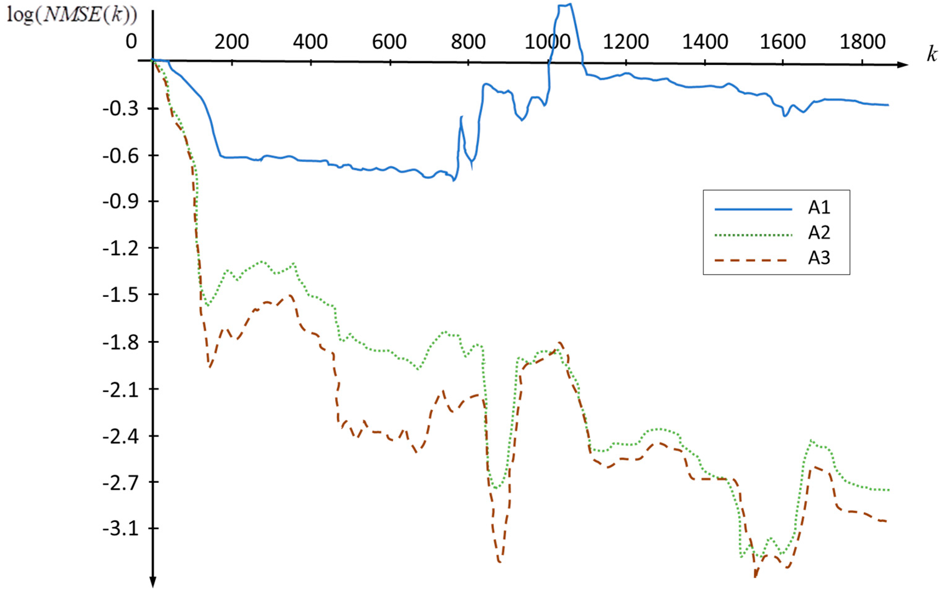
The effects of making the parameter estimates insensitive to outliers, contaminating the mainly Gaussian-distributed data, are presented in Figure 1, depicting the normalized mean square error, N M S E , defined by
N M S E k = 1 M j = 1 M θ ^ j k θ * 2 θ * 2 ;     k = 1 , , N ;   N M S = 1 N k = 1 N N M S E k
where N M S represents the average performance measure.
The N M S E estimation quality measure is calculated by using M = 100 Monte Carlo runs and N = 2000 steps. Here, is the Euclidean norm, while θ j k is the parameter vector estimate at the k-th stage for the j-th Monte Carlo run, and θ * is the true parameter vector in (49).
Figure 2 depicts the typical behavior of the analyzed algorithms under a single Monte Carlo trial ( M = 1 ).
The effects of desensitizing the parameter estimates with respect to outlier statistics, involving levels and contamination degrees of impulsive noise contaminating the predominantly Gaussian-distributed observations, are illustrated in Table 5, Table 6 and Table 7, depicting the average square error norm—the NMSE in (50)—on the basis of 100 Monte Carlo trials.
In particular, Table 8 shows the dependence of the estimate quality on the tuning parameter k δ characterizing the nonlinear influence function ψ * in (34). Since the δ -contamination degree in (40) is not known in practice, one has to adopt the k -parameter value in advance (see Table 1).
The simulation results confirm the previous conclusions drawn from the asymptotic theoretical analysis (see Table 1, Table 2 and Table 3). In this sense, the linear RLS algorithm A1 under purely Gaussian-distributed observations with δ = 0 in (40) ensures slightly better estimation quality than the AML-based recursive nonlinear identification algorithms, A2 and A3, optimal on the class in (40) (see Table 2 and Table 6). On other hand, algorithms A2 and A3 exhibit practical robustness, meaning that these algorithms are very effective in suppressing the effects of different types of outlying data points under the contamination degree 0 < δ 0.2 (see Table 3, Table 5, Table 6 and Table 7). Moreover, algorithms A2 and A3 produce comparable results, presenting a good balance between estimation quality and insensitivity to multiple outliers (see Table 5, Table 6 and Table 7). Furthermore, Table 8 shows that the nonlinear algorithms A2 and A3 are rather insensitive to the value of the saturation level k belonging to the interval 1 < k 3 .
The good results obtained by algorithms A2 and A3 are due to the adequate nonlinear processing of prediction errors through the 1.5 Huber M-robust influence function ψ * in (43) within the parameter update recursion (14). This estimation procedure is also combined with the robust recursive scheme to calculate the gain matrix Γ i in (16), based on either the fixed factor α * in (46) or the variable factor α k in (34). This, in turn, keeps the gain matrix Γ k at values high enough to ensure the fast convergence of the estimates, but also at small enough values to ensure low sensitivity to outliers. In contrast, the RLS-type algorithm A1 is inferior to the nonlinear algorithms A2 and A3 in the presence of outliers corrupting the predominantly Gaussian-distributed data.
However, algorithms A2 and A3, which are optimal on the class in (40), are nonlinear; hence, their parameter estimates may be highly sensitive to the initial choices of θ ^ 0 and Γ 0 . In general, Algorithm A3 converges slowly for higher values of Γ 0 due to the influence of the dynamics of the variable factor α k . This factor represents the current slope of the ψ * -nonlinearity in (43), which is further used to calculate the gain matrix Γ k in (16). Thus, the large residual samples in the initial steps, induced by the initial value Γ 0 , lead to a very slow decrease in the gain Γ k since the ψ * -nonlinearity operates in the saturation mode, causing the current slope α k to be close to zero. This, in turn, ensures a cumulative effect, resulting further in the slow convergence of the parameter estimates. In contrast, Algorithm A2 is found to be relatively insensitive to the value of Γ 0 due to the effect of the fixed factor α . This factor represents the average slope of ψ * -nonlinearity in (43) and is further used to calculate the gain Γ k in (16), resulting in the smooth dynamics of the gain Γ . This, in turn, reduces the influence of the initial values on the quality of parameter estimation.
In general, the problem related to the choice of the initial conditions can be circumvented by using good starting values θ ^ 0 and Γ 0 , generated, for example, by a non-recursive Huber M-robust parameter estimator [15,23,24,25,38].
Finally, the computational complexity of the developed nonlinear algorithms A2 and A3 is slightly higher than that of the linear Algorithm A1. This result is achieved at the cost of limiting the condition related to the choice of the ARX model characterized by zero-mean wide-sense stationary process noise.

8. Conclusions

This paper has addressed the problem of robust recursive parameter identification for linear discrete-time stochastic systems operating under uncertain, potentially non-Gaussian disturbance statistics. To this end, a new class of nonlinear recursive algorithms of an approximate Newton–Raphson type for parameter identification in a linear discrete-time dynamic stochastic system, excited by zero-mean white stochastic disturbances, has been developed. Strong consistency and the convergence of the asymptotic estimation errors to a zero-mean normal pdf have been established by utilizing the martingale theory approach. Starting from the Cramér–Rao theorem and the derived covariance matrix of the asymptotic estimation error, the ML-type optimal nonlinear residual transformation under a fully known noise pdf is derived. This, in turn, leads to an asymptotically efficient ML-based recursive identification algorithm, with the asymptotic estimation error covariance matrix achieving the Cramér–Rao lower bound. The link between the ML-based optimal nonlinearity and the gain matrix calculation is established through the statistical linearization coefficient, representing the expected slope of the nonlinearity. The case of disturbance uncertainty has been considered by utilizing the available prior statistical information to specify a class of pdfs to which the real unknown observation noise pdf belongs, leading to the ML-based recursive parameter identification algorithm that is optimal on a class. The proposed design provides the minimum asymptotic estimation error covariance matrix under the least favorable or worst-case pdf within the adopted class; this covariance matrix is simultaneously the maximum one within the class. Unfortunately, the min–max optimal design may be indeterminable, since an exact solution for the worst-case pdf does not generally exist. In particular, it exists only for static regression plants and FIR linear dynamic stochastic systems. The matrix optimization procedure for finding the worst-case pdf reduces to minimizing the scalar Fisher information within the specified class. Furthermore, in the case of IIR linear dynamic systems, the exact numerical solution for the worst-case pdf exists only for a class of zero-mean symmetric pdfs with finite variance. Therefore, the derived worst-case pdf solution, minimizing the Fisher information, represents an approximate optimal worst-case pdf. This, in turn, leads to an approximate ML (AML) design on a class. In addition, the ML-based optimal- and AML-based optimal-on-a-class algorithms have the same recursive nonlinear structure as the Newton–Raphson-type method, where the only difference is in the optimization procedure to find either the optimal or suboptimal worst-case one. Moreover, the proposed AML-based design on a class is step-by-step optimal, minimizing the conditional estimation error covariance matrix at each stage under the suboptimal worst-case pdf. In particular, a class of δ -contaminated Gaussian pdfs is of special importance in practice, since various scientific and industrial real measurements contain unavoidable outliers, corrupting the predominantly Gaussian-distributed measurements. In this sense, the AML-based suboptimal nonlinearity on the above class coincides with the influence functions of the Huber M-robust estimation of the location parameter, which also makes the AML-based design on the class robust in the practical sense, involving both efficiency and resistance robustness properties. However, the developed M-robustified version of the AML-based optimal on the given class design is still indeterminable, since the statistical linearization coefficient in Newton–Raphson-type recursion represents the unknown expected slope of the Huber M-robust influence function. A reasonable approach is to calculate the mathematical expectation by utilizing the AML-based suboptimal worst-case pdf, resulting in a fixed coefficient. Additionally, since such an approximation requires exact knowledge of the δ -contamination degree, a more suitable approach is to approximate the expectation via the current measurement residual realization, producing a variable coefficient.
Simulation results have shown that the proposed M-robustified AML-based optimal-on-a-class design ensures a good balance between estimation quality and insensitivity to multiple outliers, up to a contamination degree no greater than twenty percent. For higher levels of outliers, the specified class of δ -contaminated Gaussian pdfs is no longer adequate.
It is worth relating the proposed design to the ML-type parameter estimation procedures commonly used for ARMA, ARIMA, ARIMAX and GARCH models. In the ARMA(X) case, the moving-average noise term makes the one-step predictor nonlinear in the parameters, so that the conditional ML estimate is computed by iterative Gauss–Newton-type optimization or, recursively, by the recursive prediction error method (RPEM) [11,12]. The ARIMA(X) family additionally treats nonstationarity through differencing, while GARCH models describe conditionally heteroskedastic disturbances, estimated in practice by the quasi-ML approach. All these procedures rely on the Gaussian, or conditionally Gaussian, likelihood and are therefore sensitive to heavy-tailed disturbances and outliers in the same way as the RLS algorithm analyzed here. The ARX equation error structure with i.i.d. disturbances, adopted in this paper, represents the case in which the regression vector is measurable with respect to σ -algebra generated by the past input–output data, enabling the rigorous martingale-based convergence analysis, as well as the explicit M-robustified AML design on a class. Within this framework, RPEM essentially reduces to the RLS algorithm, so that the presented comparisons implicitly cover the corresponding ML-type benchmark.
Further investigations should be oriented towards designing an AML-based recursive identification algorithm, optimal on a class, under levels of prior information on stochastic disturbances that differ from those assumed here, involving correlated noise within the ARMA and ARMAX model structures (e.g., by M-robustifying the RPEM recursion); conditionally heteroskedastic disturbances of the GARCH type, with unequally distributed observations; asymmetric noise pdfs, etc. Some preliminary results may be found in the statistical literature, but their application to the dynamic system identification problem requires further work.

Author Contributions

Conceptualization, Z.B. and B.K.; methodology, Z.B., T.U. and B.K.; software, M.Ž. and M.P.; validation, Z.B. and B.K.; formal analysis, M.Ž. and M.P.; writing—original draft, Z.B., T.U. and B.K.; visualization, M.Ž. and M.P.; supervision, Z.B. and B.K. All authors have read and agreed to the published version of the manuscript.

Funding

This research received no external funding.

Data Availability Statement

The original contributions presented in this study are included in the article. Further inquiries can be directed to the corresponding author.

Conflicts of Interest

The authors declare no conflicts of interest.

Abbreviations

The following abbreviations are used in this manuscript:
A1Linear RLS optimal under the standard Gaussian pdf
A2AML identification algorithm, optimal on the class, with fixed coefficient
A3AML identification algorithm, optimal on the class, with variable coefficient
AMLApproximate ML
a.sAlmost surely
ARXAutoregressive with exogenous input
BIBOBounded input–bounded output
CRCramér–Rao
EEEquation error
FIRFinite impulse response
i.i.d.Independent and identically distributed
IIRInfinite impulse response
LS Least squares
MADMedian absolute deviation
MLMaximum likelihood
MMSEMinimum mean square error
NMSENormalized mean square error
ODEOrdinary differential equation
pdfProbability density function
w.p.1With probability one

Appendix A

Proof of Theorem 2. 
Let us denote the estimation error by θ ˜ i = θ ^ i θ * and rewrite the algorithm (14)–(16) in the form
θ ^ i = θ ^ i 1 + R ¯ 1 i Z i ψ ε i , θ ^ i 1
R ¯ i = R ¯ i 1 + α Z i Z T i ; α = E p ψ
where E p is the expectation with respect to the noise pdf p , while Γ i = R ¯ 1 i . Taking into account (A1) and (A2), one obtains
R ¯ i θ ˜ i = R ¯ i 1 θ ˜ i 1 + α Z i Z T i θ ˜ i 1 + Z i ψ ε i , θ ^ i 1
By summarizing (A3) from 0 to i , it further follows that
R ¯ i θ ˜ i = R ¯ 0 θ ˜ 0 + k = 1 i α Z k Z T k θ ˜ k 1 + Z k ψ ε k , θ ^ k 1
The relation (A4) can be rewritten in the form
R ¯ i θ ˜ i = R ¯ 0 θ ˜ 0 + k = 1 i Z k ψ e k + k = 1 i Z k α Z T k θ ˜ k 1 + ψ ε k , θ ^ k 1 ψ e k
Moreover, by introducing R ¯ i = i R i , it follows from the relation (A5) that
i θ ˜ i = 1 i R 1 i R ¯ 0 θ ˜ 0 + 1 i R 1 i k = 1 i Z k ψ e k + 1 i R 1 i k = 1 i Z k α Z T k θ ˜ k 1 + ψ ε k , θ ^ k 1 ψ e k
Since the influence of the initial guess θ ^ 0 on the parameter vector θ * vanishes as the time index i increases, it suffices to analyze the last two terms on the right-hand side of (A6). Thus, to investigate the influence of the third term in (A6), let us analyze the expression
Z k α Z T k θ ˜ k 1 + ψ ε k , θ ^ k 1 ψ e k   Z k       α Z T k θ ˜ k 1 + ψ ε k , θ ^ k 1 ψ e k  
where denotes the Euclidean norm, and denotes the absolute value. By linearizing the nonlinearity ψ ε k , θ in the vicinity of the true parameter vector θ * using the truncated Taylor series expansion, and taking θ = θ ^ k 1 , one obtains
ψ ε k , θ ^ k 1 ψ e k + ψ e k Z T k θ ˜ k 1 = 1 2 ψ e k Z T k θ ˜ k 1 2
By applying hypothesis H5, one concludes that ψ k 1 and ψ k 2 , yielding further from (A8)
ψ ε k , θ ^ k 1 ψ e k + k 1 Z T k θ ˜ k 1 k 2 Z T k θ ˜ k 1 2
for some positive constants k 1 , 2 0 , . Since, under hypothesis H3, the generated data are bounded, one gets from (A7)–(A9)
Z k α Z T k θ ˜ k 1 + ψ ε k , θ ^ k 1 ψ e k   k 3 θ ˜ k 1 2
where k 3 is a finite positive constant. Next, let us analyze the random vector
S i = k = 1 i k   1 2   δ Z k ψ e k = S i 1 + i   1 2   δ Z i ψ e i
Furthermore, since E ψ e k = 0 , owing to hypotheses H2 and H4, one further obtains
E S i F i 1 = E k = 1 i k   1 2   δ Z k ψ e k F i 1 + i   1 2   δ Z i E ψ e i   = S i 1
On the other hand, one gets from (A11)
S i 2 = k = 1 i k   1 2   δ 2 Z k 2 ψ e k   2
By applying the unconditional expectation operator E on (A13) and taking into account hypotheses H2–H4, one concludes that the random quantities Z k and ψ e k are bounded and uncorrelated, yielding
E S i   2 = k = 1 i k   1 2   δ 2 E   Z k 2 E   ψ e k   2 k 4 k = 1 k 1 2 δ <
for some positive constant k 4 0 , . The last inequality follows from the Cauchy integral criterion, stating that the sequence k = 1 k l for l > 1 converges [45]. Thus, under relations (A12) and (A14), one concludes that the vector discrete-time stochastic process S i is a martingale sequence, so that the basic martingale convergence theorem from Lemma 4 implies that [43]
lim i S i = S < ,     w . p . 1
Taking into account Lemma 3, with the choice x k = Z k ψ e k and b k = k   1 2   δ , one also gets [45]
lim i     i   1 2   δ   k = 1 i k   1 2   δ Z k ψ e k = 0 ,     w . p . 1
Furthermore, one obtains from relation (A6)
i θ ˜ i = R 1 i R ¯ 0 θ ˜ 0 + R 1 i i 1 2   +   δ 1 i 1 2   +   δ k = 1 i Z k ψ e k + R 1 i k = 1 i Z k α Z T k θ ˜ k 1 + ψ ε k , θ ˜ k 1 ψ e k
Under hypothesis H6 and relations (A10), (A16) and (A17), one gets
i θ ˜ i R 1 i R 0 θ ˜ 0 + k 5 R 1 i i 1 2   +   δ + k 3 R 1 i   k = 1 i θ ˜ k 1 2 k 6 + k 7 i 1 2   +   δ + k 8 k = 1 i θ ˜ k 1 2 k 9 i 1 2   +   δ + k = 1 i θ ˜ k 1 2
for some positive constants k j 0 , , j = 5 , 6 , , 9 . By substituting into Lemma 1 b i = θ ˜ i and α 1 = 1 / 2 + δ , yielding β = max 0 , 2 δ , as well by applying Lemma 1 to relation (A18), one obtains
k = 1 i θ ˜ k 1 2 k 9 i 2 δ
In this way, due to relations (A10) and (A19), the third term on the right-hand side of (A6) satisfies
1 i R 1 i k = 1 i Z k α Z T k θ ˜ k 1 + ψ ε k , θ ^ k 1 ψ e k R 1 i 1 i k 3 k 9 i 2 δ k 10 1 i 1 / 2 2 δ     i     0
where k 10 is a finite positive constant, and 1 / 2 2 δ > 0 . Taking into account (A20), one concludes that the asymptotic distribution of the estimation error only depends on the second addends in (A6). Furthermore, to find the expression for the underlying asymptotic estimation error distribution, let us apply Lemma 2 to each component of the random vector
x k = x j k d × 1 = 1 i k = 1 i Z k ψ e k ;   x j k = Z j k ψ e k ;   j = 1 , , d ,   d = n + m
where Z j k is the j-th component of the d × 1 information vector Z k in (5). In addition, starting from the scalar components x j k of the vector x k in (A21), one can write x j 2 k = x j k x j T k , from which follows the matrix quantity
V n 2 = E x j 2 k   F k 1 d × d = k = 1 n E Z j k ψ e k 2   F k 1 d × d = k = 1 n Z k Z T k E ψ 2 e k
and the underlying expected value of the above matrix quantity
S n 2 = E V n 2 = k = 1 n E Z k Z T k E ψ 2 e k
Here, we use the fact that the scalar white observation noise sequence e k is uncorrelated with the past observations, within the d × 1 information vector Z k in (5). Furthermore, by applying the law of large numbers to relations (A22) and (A23), one obtains [10]
V n 2 n   n E Z k Z T k E ψ 2 e k
S n 2 n   n E Z k Z T k E ψ 2 e k
Thus, starting from the matrices in (A24) and (A25), and applying Lemma 2 to each of the components of these matrices, one concludes that the first condition of Lemma 2 is fulfilled. Moreover, since lim n S n = , due to (A23), and since the vector quantity Z k ψ e k in (A21) is bounded by hypotheses H3 and H4, one obtains the scalar ratio for each component j of the matrices (A24) and (A25):
1 S n j 2 k = 1 n E Z j k ψ e k 2 P Z j k ψ e k   > ε S n j   n 0 ;   j = 1 , , d
Thus, taking into account the relations in (A26), one concludes that the second condition of Lemma 2 is also is fulfilled. Again, by applying Lemma 2 to the components of the matrix (A21), one concludes that
1 i k = 1 i Z k ψ e k D N 0 , Q ;     Q = E Z k Z T k E ψ 2 e k
where N 0 , Q is the multidimensional zero-mean normal pdf with the covariance matrix Q , while the symbol “ D ” designates the asymptotic convergence in distribution. Taking into account relation (A2), and the fact that R ¯ i = i R i , it further follows that
R i = 1 i R ¯ 0 + 1 i k = 1 i α Z i Z T i
Moreover, by applying the law of large numbers to (A28), one gets
R i i R = E α Z i Z T i = E ψ e i E Z i Z T i
where the linearization coefficient α = E ψ e i due to (14) [10]. In addition, from hypothesis H3 and relations (A27) and (A29), one obtains the relations
1 i R 1 i k = 1 i Z k ψ e k D N 0 , V ; V = R 1 Q R 1
Finally, by substituting (A30) into (A17), and neglecting the influence of the initial conditions for a sufficiently large discrete-time index i , one obtains the relations in (17), which completes the proof. □

References

  1. Kashyap, R.L.; Rao, A.R. Dynamic Stochastic Models from Empirical Data; Academic Press: New York, NY, USA, 1976. [Google Scholar]
  2. Goodwin, G.C.; Payne, R.L. Dynamic System Identification: Experimental Design and Data Analysis; Academic Press: New York, NY, USA, 1977. [Google Scholar]
  3. Sinha, N.K.; Kuszta, B. Modeling and Identification of Dynamic Systems; Van Nostrand Reinhold Co.: New York, NY, USA, 1983. [Google Scholar]
  4. Schoukens, J.; Pintelon, R. Identification of Linear Systems: A Practical Guideline to Accurate Modeling, 1st ed.; Pergamon Press: Oxford, UK, 1991. [Google Scholar]
  5. van den Bosch, P.P.J.; van der Klauw, A.C. Modeling, Identification and Simulation of Dynamical Systems; CRC Press: Boca Raton, FL, USA, 2020. [Google Scholar]
  6. Candy, J.V. Model–Based Signal Processing; Wiley–IEEE Press: Hoboken, NJ, USA, 2010. [Google Scholar]
  7. van der Heijden, F.; Lei, B.; Xu, G.; Ming, F.; Zou, Y.; de Ridder, D.; Tax, D.M. Classification, Parameter Estimation, and State Estimation: An Engineering Approach Using MATLAB, 2nd ed.; John Wiley & Sons: Hoboken, NJ, USA, 2017. [Google Scholar]
  8. Verhaegen, M.; Vincent, V. Filtering and System Identification: A Least Square Approach; Cambridge University Press: Cambridge, UK, 2017. [Google Scholar]
  9. Kovačević, B.; Đurović, Ž.; Banjac, Z. Fundamentals of Stochastic Signals, Systems and Estimation Theory with Worked Examples, 3rd ed.; Springer: Cham, Switzerland, 2026. [Google Scholar]
  10. Papoulis, A.; Pillai, S.U. Probability, Random Variables, and Stochastic Processes, 4th ed.; McGraw–Hill: New York, NY, USA, 2021. [Google Scholar]
  11. Ljung, L.; Söderström, T. Theory and Practice of Recursive Identification, 3rd ed.; MIT Press: Cambridge, MA, USA, 1986. [Google Scholar]
  12. Ljung, L. System Identification: Theory for the User, 2nd ed.; Prentice Hall PTR: Upper Saddle River, NJ, USA, 2012. [Google Scholar]
  13. Goodwin, G.C.; Sin, K.S. Adaptive Filtering Prediction and Control, Dover ed.; Dover Publications: Mineola, NY, USA, 2014. [Google Scholar]
  14. Mendel, J.M. Discrete Techniques of Parameter Estimation: The Equation Error Formulation; M. Dekker: New York, NY, USA, 1973. [Google Scholar]
  15. Tsypkin, Y.Z. Foundations of the Information Theory of Identification; Nauka: Moscow, Russia, 1984. [Google Scholar]
  16. Box, G.E.P.; Jenkins, G.M.; Reinsel, G.C. Time Series Analysis: Forecasting and Control, 4th ed.; John Wiley & Sons: Hoboken, NJ, USA, 2008. [Google Scholar]
  17. Åström, K.J.; Wittenmark, B. Computer-Controlled Systems: Theory and Design, 3rd ed.; Dover Publications: Mineola, NY, USA, 2011. [Google Scholar]
  18. Markel, J.D.; Gray, A.H., Jr. Linear Prediction of Speech; Springer: Berlin/Heidelberg, Germany, 1976. [Google Scholar]
  19. Rabiner, L.R.; Schafer, R.W. Theory and Applications of Digital Speech Processing; Pearson: Upper Saddle River, NJ, USA, 2011. [Google Scholar]
  20. Childers, D.G. (Ed.) Modern Spectrum Analysis; IEEE Press: New York, NY, USA, 1978. [Google Scholar]
  21. Haykin, S. Adaptive Filter Theory, 4th ed.; Pearson India: Delhi, India, 2008. [Google Scholar]
  22. Sayed, A.H. Fundamentals of Adaptive Filtering; Wiley–IEEE Press: Hoboken, NJ, USA, 2003. [Google Scholar]
  23. Kovačević, B.; Banjac, Z.; Milosavljević, M. Adaptive Digital Filters; Springer: Berlin/Heidelberg, Germany, 2013. [Google Scholar]
  24. Poljak, B.T.; Tsypkin, J.Z. Robust identification. Automatica 1980, 16, 53–63. [Google Scholar] [CrossRef] [Scilit]
  25. Tsypkin, Y.Z. Optimality in identification of linear plants. Int. J. Syst. Sci. 1983, 14, 59–74. [Google Scholar] [CrossRef] [Scilit]
  26. Noton, A.R.M. Introduction to Variational Methods in Control Engineering; Pergamon Press: Oxford, UK, 1965. [Google Scholar]
  27. Bellman, R. Dynamic Programming; Princeton University Press: Princeton, NJ, USA, 2010. [Google Scholar]
  28. Pontrjagin, L.S.; Gamkrelidze, R.V. Selected Works, Vol. 4: The Mathematical Theory of Optimal Processes; Gordon and Breach: New York, NY, USA, 1986. [Google Scholar]
  29. Adby, P.R.; Dempster, M.A.H. Introduction to Optimization Methods; Chapman and Hall: London, UK, 1982. [Google Scholar]
  30. Dixon, L.C.W. Nonlinear Optimisation; English Universities Press: London, UK, 1972. [Google Scholar]
  31. Chapra, S.C.; Canale, R.P. Numerical Methods for Engineers, 8th ed.; McGraw-Hill Education: New York, NY, USA, 2021. [Google Scholar]
  32. Barnett, V.; Lewis, T. Outliers in Statistical Data, 3rd ed.; Wiley: Chichester, UK, 2000. [Google Scholar]
  33. Venables, W.N.; Ripley, B.D. Modern Applied Statistics with S, 4th ed.; Springer: New York, NY, USA, 2002. [Google Scholar]
  34. Wilcox, R.R. Introduction to Robust Estimation and Hypothesis Testing, 5th ed.; Academic Press: San Diego, CA, USA, 2022. [Google Scholar]
  35. Huber, P.J.; Ronchetti, E.M. Robust Statistics, 2nd ed.; Wiley: Hoboken, NJ, USA, 2013. [Google Scholar]
  36. Kovačević, B.; Banjac, Z.; Unkašević, T. Perspective Chapter: Approximate Kalman Filter using M-robust Estimate Dynamic Stochastic Approximation with Parallel Adaptation of Unknown Noise Statistics by Huber’s M-robust Parameter Estimator. In Kalman Filters—Theory, Applications, and Optimization; Khalid, A., Sarwat, A.I., Riggs, H., Eds.; IntechOpen: London, UK, 2024. [Google Scholar] [CrossRef] [Scilit]
  37. de Menezes, D.Q.F.; Prata, D.M.; Secchi, A.R.; Pinto, J.C. A review on robust M-estimators for regression analysis. Comput. Chem. Eng. 2021, 147, 107254. [Google Scholar] [CrossRef] [Scilit]
  38. Kovacevic, B.; Milosavljevic, M.M.; Veinović, M.; Marković, M. Robust Digital Processing of Speech Signals; Springer International Publishing: Cham, Switzerland, 2018; Softcover reprint of the original 1st ed. 2017. [Google Scholar]
  39. Hampel, F.R.; Ronchetti, E.M.; Rousseeuw, P.J.; Stahel, W.A. Robust Statistics: The Approach Based on Influence Functions; Wiley: Hoboken, NJ, USA, 2011. [Google Scholar]
  40. Lai, T.L.; Wei, C.Z. Least squares estimate in stochastic regression models with applications to identification and control of dynamic systems. Ann. Stat. 1982, 10, 154–166. [Google Scholar] [CrossRef] [Scilit]
  41. Kovacevic, I.; Kovacevic, B.; Djurovic, Z. On strong consistency of a class of recursive stochastic Newton–Raphson type algorithms with application to robust linear dynamic system identification. Facta Univ. Ser. Electron. Energ. 2008, 21, 1–21. [Google Scholar] [CrossRef] [Scilit]
  42. Willems, J.L. Stability Theory of Dynamical Systems; Wiley: New York, NY, USA, 1970. [Google Scholar]
  43. Neveu, J. Discrete-Parameter Martingales; North-Holland: Amsterdam, The Netherlands, 1975. [Google Scholar]
  44. Hall, P.; Heyde, C.C.; Birnbaum, Z.W.; Lukacs, E. Martingale Limit Theory and Its Application; Elsevier Science: Amsterdam, The Netherlands, 2014. [Google Scholar]
  45. Knopp, K. Infinite Sequences and Series; Dover Publications: Mineola, NY, USA, 2009. [Google Scholar]
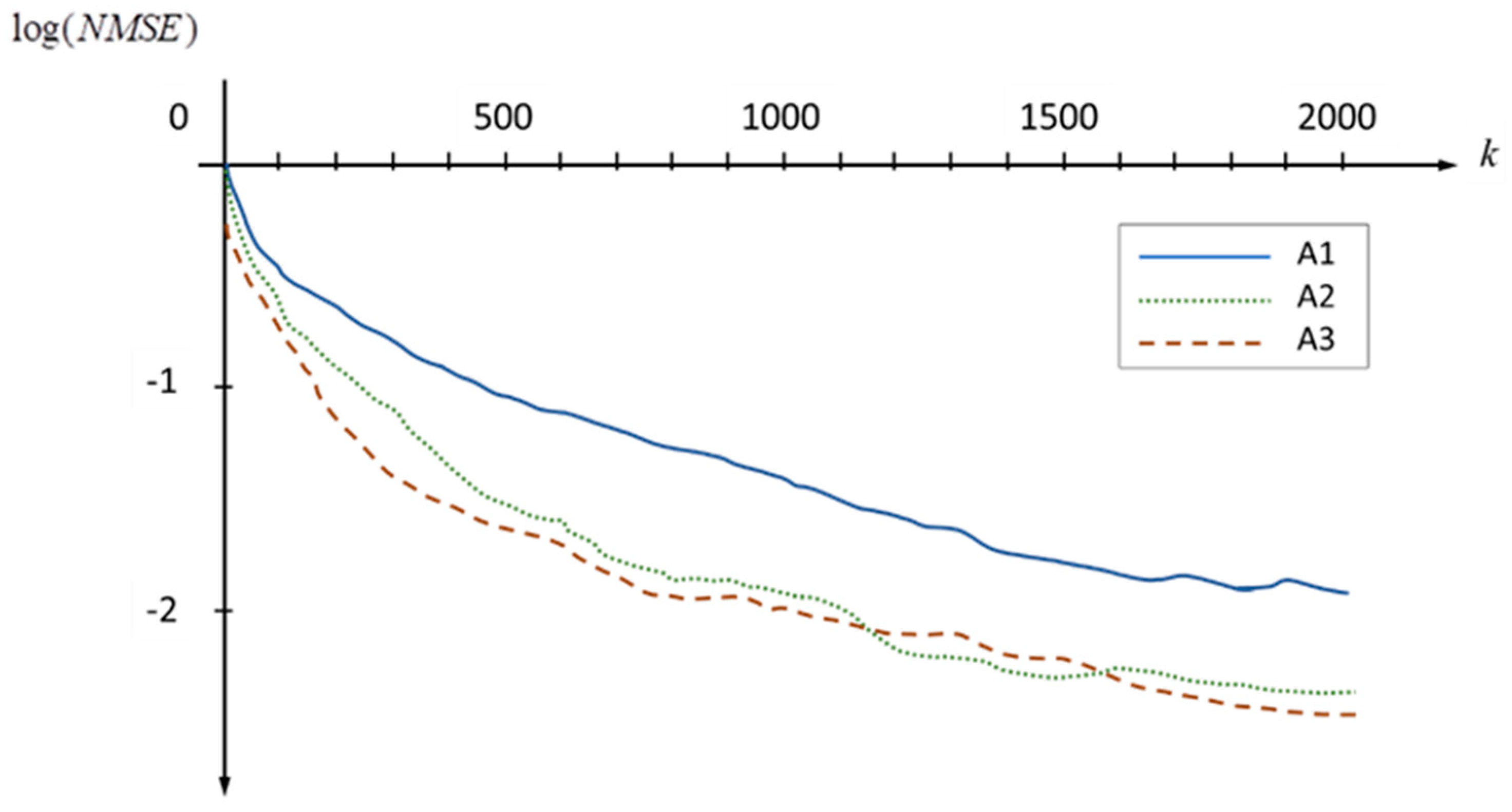
Figure 1. Normalized mean square error norm, N M S E in (50), based on M = 100 Monte Carlo runs for different algorithms under a Gaussian mixture noise pdf, (40), with statistical parameters δ = 0.1 , p 0 = N | 0 , 100 (initial conditions θ ^ 0 = 0 , Γ 0 = 0.1 I ).
Mathematics 14 02663 g001
Figure 2. Normalized mean square error norm, (50), based on a single Monte Carlo run ( M = 1 ) for different algorithms under a Gaussian mixture noise pdf, (40), with statistical parameters δ = 0.1 , p 0 = N | 0 , 100 (initial conditions θ ^ 0 = 0 , Γ 0 = 0.1 I ).
Mathematics 14 02663 g002
Table 1. Dependence of tuning parameter k δ in (43) on δ -contamination degree in (40).
δ 0.000.010.020.050.100.200.501.00
k δ 2.001.701.401.100.900.400.00
Table 2. Dependence of R A E F criterion (48) on δ -contamination degree in (40).
δ 0.000.010.020.050.100.200.501.00
R A E F 0.870.860.850.820.780.740.690.43
Table 3. RAEF criterion (48) for various observation noise statistics.
R A E F Criterion in (48)
p d f N 0 , 2 R 2 , 2 L 0 , 0.5 C 0 , 1 δ = 0.1 ,     p 0 = N 0 , 10 in (40)
σ 2 2.001.332.0 10.9
I p 0.500.06250.250.500.80
R A E F 1.6013.903.201.601.09
Algorithm: θ ^ ρ : (14)–(16), (43) and (46), k = 1.5 , δ = 0.1
Description: p —noise pdf; σ 2 —variance; I p —Fisher information
N z | 0 , σ 2 = 1 / 2 π σ exp z 2 / 2 σ 2 zero-mean normal pdf; I p = σ 2
R a , b —uniform pdf on interval a , b ; σ 2 = b a 2 / 12 ; I p = 1 / b a 2
L z | 0 , λ = λ / 2 exp λ z zero-mean Laplace; σ 2 = 2 / λ 2 , I p = λ 2
C 0 , λ = λ / π λ 2 + z 2 1 zero-mean Cauchy pdf, σ 2 = .
Table 4. Flowchart of Algorithm A3 with variable linearization coefficient.
Step 0:
 Set the initial values: θ ^ 0 in (14); Γ 0 in (16); threshold level k in (41); nominal noise variance σ n 2 in (40); polynomial orders n and m in (2), n m ; number of iterations N s ; initial regression vector in (3), Z T n = y n 1 , , y 0 , u n 1 , , u n m ;
 Define influence function ψ * in (41) for the given k value.
Step 1: Time-counter initialization, i = n ; θ ^ n 1 = θ ^ 0 ; Γ n 1 = Γ 0
Step 2: Calculate the measurement residual in (14), ε i = y i Z T i θ ^ i 1
Step 3: Calculate the residual nonlinear transformation ψ i = ψ * ε i
Step 4: Calculate the variable linearization factor α in (34), α i = ψ i ε i     if     ε i 0 1                                     if     ε i = 0
Step 5: Calculate the gain matrix from (16), Γ i = Γ i 1 Γ i 1 Z i Z T i Γ i 1 α i 1 + Z T i Γ i 1 Z i
Step 6: Calculate the parameter estimate update θ ^ i = θ ^ i 1 + Γ i Z i ψ i
Step 7: Increase time counter i i + 1
Step 8:
  IF i N S THEN
   Memorize the parameter estimates θ ^ i ,
   Take the current input–output signals y i ,     u i ,
   Upgrade the regression vector Z T i = y i 1 , , y i n , u i 1 , , u i m ,
   where y j = 0 , u j = 0 for j < 0
   GOTO Step 2
  ENDIF
End of the simulation
Note: The flowchart describes the nonlinear Algorithm A3. If the fixed linearization coefficient α in (46) is used instead of the variable coefficient, the flowchart reduces to Algorithm A2; if the fixed coefficient is chosen to be α = 1 , and the linear transformation ψ x = x is used instead of the nonlinear one in (41), the flowchart reduces to the RLS algorithm.
Table 5. The N M S criterion (50) for different algorithms and various outlier statistics in (40).
pdf
δ = 0.1 δ = 0.1 δ = 0.1 δ = 0.1
p 0 = C 0 , 1 p 0 = R 5 , 5 p 0 = L 0 , 1 p 0 = N 0 , 10
Algorithm
A11.1950.1050.1770.104
A20.0820.0190.0620.029
A30.0810.0510.0640.029
Table 6. Average mean square error norm for different algorithms as a function of the outlier probability, with θ ^ 0 = 0 , Γ 0 = 0.1 I , k = 1.5 , σ n 2 = 1 , p 0 = N | 0 , 10 .
pdf in (40)
δ = 0 δ = 0.02 δ = 0.03 δ = 0.05 δ = 0.1 0
Algorithm
A10.0200.0530.0710.0860.104
A20.0400.0260.0300.0280.029
A30.0380.0260.0300.0250.029
Table 7. Average mean square error norm for different outlier intensities with θ ^ 0 = 0 , Γ 0 = 0.1 I , k = 1.5 , σ n 2 = 1 , δ = 0.1 for different algorithms.
pdf
p 0 = N | 0 , 3 p 0 = N | 0 , 6 p 0 = N | 0 , 10
Algorithm
A10.0490.0830.117
A20.0240.0260.040
A30.0240.0270.040
Table 8. Average mean square error norm for different algorithms, as a function of saturation level k , with δ = 0.1 , p 0 = N | 0 , 10 , θ 0 = 0 , Γ 0 = 0.1 I .
k
k = 1.0 k = 1.5 k = 2.0 k = 3.0 k = 4.0
Algorithm
A20.0300.0280.0280.0330.042
A30.0300.0280.0280.0320.041
Disclaimer/Publisher’s Note: The statements, opinions and data contained in all publications are solely those of the individual author(s) and contributor(s) and not of MDPI and/or the editor(s). MDPI and/or the editor(s) disclaim responsibility for any injury to people or property resulting from any ideas, methods, instructions or products referred to in the content.