Research on Enterprise Financial Distress Warning Based on Residual GRU Model

Abstract

In the context of increasing global economic uncertainty, the financial risks of listed companies exhibit significant dynamic evolution characteristics. Traditional methods based on static indicators are no longer sufficient to meet the requirements of forward-looking early-warning. Considering the intertemporal transmission and path dependence characteristics of enterprise financial risks, from the perspective of deep temporal modeling, this study constructs a Gated Recurrent Unit model (Residual GRU, RGRU) that integrates a residual connection mechanism to enhance the feature transmission ability in the deep network and alleviate the problem of gradient propagation difficulties. Taking Chinese A-share listed companies from the first quarter of 2010 to the fourth quarter of 2024 as the research sample, and using the Special Treatment (ST) or Delisting Risk Warning (*ST) status as the distress determination criterion, an enterprise financial distress early-warning system is constructed based on multi-dimensional financial and corporate governance indicators. On this basis, ablation experiments are set up from two dimensions—the type of recurrent units (GRU and LSTM) and the connection mechanism (residual connection and dense connection)—and performance is evaluated through systematic parameter optimization and multi-layer network structure experiments. The empirical results show that the RGRU model outperforms the comparison model in classification indicators such as accuracy, F1 score, recall, and probability prediction indicators such as Brillouin score and logarithmic loss, and demonstrates better stability and generalizability. The research results indicate that the introduction of residual connections can effectively improve the prediction performance and practical value of recurrent neural networks in the enterprise financial distress early-warning task.

1. Introduction

Enterprise financial distress prediction is at the core of financial risk management, aiming to dynamically model reality based on historical data to identify potential risks. Given the dynamic continuity of financial data, risks are often hidden within long-term trends such as rising debt ratios or long-term negative cash flows. Therefore, constructing a predictive model that can capture cross-cycle dependencies has become a key issue.

Early studies on financial distress prediction primarily relied on statistical approaches and depended on financial ratios as explanatory variables [1]. Representative models include the Altman Z-score, which constructs a linear combination of financial indicators through discriminant analysis, and the logistic regression model, which estimates the probability of financial distress based on firm-specific characteristics [2,3]. Although these models provide useful insights for enterprise risk assessment, their effectiveness is limited by methodological assumptions such as the reliance on linear relationships, and the variable selection range is mainly concentrated on financial ratios, which restricts the inclusion of non-financial or macroeconomic information. These models also struggle to capture the inherent nonlinear mechanisms and dynamic characteristics of enterprise operations.

The rise of machine learning (ML) has addressed these limitations through the introduction of outstanding nonlinear models. For instance, Bluwstein et al. (2023) used random forests, extremely randomized trees, support vector machines, and artificial neural networks to predict macroeconomic conditions across 17 countries, and found that machine learning models consistently outperformed traditional logistic regression in out-of-sample and recursive forecasts [4]. Song et al. (2023) combined K-means clustering with a backpropagation neural network to forecast risks for 136 internet finance companies, attaining an accuracy of 99.51% [5]. Ref. [6] Jan (2021) applied the Chi-square Automatic Interaction Detector (CHAID) method to select key financial features and used them as inputs for deep neural networks (DNNs) and convolutional neural networks (CNNs), and the resulting CHAID-CNN model achieved the highest accuracy (94.23%) and significantly reduced both Type I and Type II errors [6].

Traditional statistical and machine learning methods primarily depend on cross-sectional data, which limits their ability to capture temporal dependencies and long-term dynamics in financial indicators, thereby constraining their predictive power in complex and evolving environments. With the emergence of Long Short-Term Memory (LSTM) and Gated Recurrent Unit (GRU) models, which have demonstrated strong forecasting capabilities in stock price prediction, air quality forecasting, and power load prediction, researchers began exploring their application in financial distress prediction [7,8,9,10]. Ayvaz et al. (2020) integrated the Sustainable Balanced Scorecard (SBSC) with LSTM to build a risk early-warning model, achieving 95.41% accuracy in predicting the 2002 and 2008 financial crises, further confirming the superiority of LSTM in handling non-stationary economic time-series data [11]. Additionally, Yi and Yan (2023) combined wavelet decomposition and the ARIMA-GRU hybrid model to predict risks in electromechanical products [12]. These studies collectively indicate that LSTM and GRU are effective in capturing trend dynamics in financial time-series data.

However, as neural networks continue to deepen, the traditional sequential connections between layers gradually weaken or overwrite the early features due to successive nonlinear transformations. This limits the ability of deep networks to extract low-level information, increases the possibility of gradient vanishing, and thereby reduces the prediction performance. To address these issues, researchers have explored architectural enhancements such as residual and dense connections. Residual connections introduce skip links that allow shallow features to flow directly into deeper layers, facilitating identity mappings between inputs and outputs and mitigating gradient vanishing problems [13]. For instance, You et al. (2023) combined a residual structure with a multi-head attention GRU to construct an Attention ResNet-GRU model for typhoon prediction, achieving significant reductions in trajectory and intensity errors [14]. Cheng et al. (2022) integrated residual connections with LSTM for PM2.5 concentration prediction, outperforming gradient boosting and traditional RNN models [15]. Wang et al. (2025) embedded residual connections into the BSDA-Mamba model for medical image classification, combining it with Bayesian semantic data augmentation to substantially enhance the robustness of tumor image classification [16].

Unlike residual connections, dense connections establish fully connected inter-layer structures, enabling each layer to receive outputs from all preceding layers, thereby improving information flow and feature reuse efficiency [17]. Their superior performance in deep architectures has been widely verified across domains. For example, Azar et al. (2020) proposed a hybrid LSTM-DenseNet model and conducted experiments on 15 benchmark datasets, showing that the model outperformed many State-of-the-Art methods [18]. Zhi et al. (2025) incorporated attention mechanisms into a dense connection framework for driver fatigue detection tasks [19]. Guo (2025) and Lu (2025) enhanced the utilization of image feature information through dense inter-layer connections [20,21]. Parthasarathy and Santhosh (2024) developed a Dense-BiGRU model based on dense connectivity, which achieved excellent performance in ECG heart failure detection [22].

In summary, the methods for predicting enterprise financial distress have evolved from traditional statistical methods to classic machine learning approaches, and recently to deep time-series modeling. The accuracy and adaptability of these predictions have continuously improved. However, the research on the integration of existing deep time-series models with advanced network architectures is mostly concentrated in areas such as image recognition and stock index prediction. The integrated modeling of enterprise financial data is still insufficient, and related research needs further deepening. Therefore, this study takes GRU as the basic model and introduces the residual connection mechanism to enhance the information transmission ability and alleviate the problem of gradient disappearance, and constructs an improved deep learning neural network model considering the multi-dimensional and nonlinear characteristics of enterprise financial data. This study makes the following contributions:

(1)

This study is the first to extend the residual connection GRU architecture to the enterprise financial distress warning scenario. An adapted RGRU model is constructed based on the time-series financial data of A-share listed companies. The residual mechanism introduced in this study effectively alleviates the gradient disappearance problem in multi-layer time-series training, and enhances the feature expression ability and training stability of the deep financial risk prediction model.

(2)

Through the construction of a multi-dimensional ablation experiment system, the prediction performance, calibration ability, and computational efficiency of RGRU have been comprehensively verified on real enterprise financial datasets. The actual value of the residual-enhanced model in early-warning applications is highlighted.

(3)

Through empirical analysis, the relative advantages of residual connection in time-series risk control models are clarified, providing a reference for the subsequent structural design of deep time-series networks.

The organizational structure of the remaining parts of this study is as follows: Section 2 introduces the mathematical basis of the used models. Section 3 details the construction of the warning index system and data preprocessing steps. Section 4 elaborates on the design process of the model, the selection strategy of the hyperparameters, and the determination of the evaluation indicators. Section 5 conducts the empirical evaluation.

2. Model Methods

2.1. Advanced Network Architecture

2.1.1. Residual Network

ResNet is a deep neural network architecture composed of multiple residual blocks. In traditional neural networks, information is generally transmitted layer-by-layer, which maps the input $\mathit{x}$ to the desired output $H(\mathit{x})$, fitting a complex underlying mapping $H(\mathit{x})$ [13].

In contrast, the residual block utilizes skip connections to bypass multiple network layers and directly propagate the input $\mathit{x}$ to subsequent layers. In this way, the network only needs to learn the residual mapping $F(\mathit{x})$ between the input and the expected output, and the overall mapping can be formulated as $H(\mathit{x})=F(\mathit{x})+\mathit{x}$, where the operator “$+$” denotes element-wise addition.

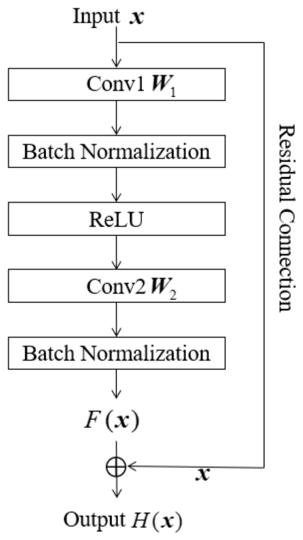
When the deep network reaches performance saturation, the architectural design enables the residual mapping to easily approximate zero, $F(\mathit{x})=0$. This ensures that deep networks can maintain high training accuracy, while effectively alleviating the problem of gradient vanishing. A complete residual block consists of two components—the main path and the residual connection—and its structural diagram is illustrated in Figure 1.

(1) Main path structure: The main path typically consists of two convolutional layers, two batch normalization layers, and a nonlinear activation layer. The convolutional layers are used to extract local features and maintain the consistency of input and output dimensions through appropriate convolution operations. The batch normalization layer standardizes the convolution results to alleviate internal covariate shift and accelerate training convergence. The nonlinear activation function is employed to introduce nonlinear expression ability. The calculation formula for the forward propagation process of the residual block is as follows:

$$F(\mathit{x})=BN({\mathit{W}}_2\sigma (BN({\mathit{W}}_1\mathit{x})))$$

(1)

$$H(\mathit{x})=F(\mathit{x})+\mathit{x}$$

(2)

In Equations (1) and (2), ${\mathit{W}}_i(i=1,2)$ are the weight matrices of the convolutional layers, $BN(\cdot )$ denotes the batch normalization operation, and $\sigma (\cdot )$ represents the Leaky ReLU activation function.

(2) Residual connection: Through identity mapping or linear transformation, residual connection performs element-wise addition between the input and the residual mapping, as denoted by the “$\oplus$” in Figure 1.

When the dimensions of the residual block input $\mathit{x}$ and the residual mapping $F(\mathit{x})$ are consistent, the identity mapping can be adopted to directly add $\mathit{x}$ and the residual mapping $F(\mathit{x})$ element-wise to obtain the expected output $H(\mathit{x})$, as shown in Equation (2).

If the dimensions of the input $\mathit{x}$ and the residual mapping $F(\mathit{x})$ do not match, a $1\times 1$ convolution is applied to adjust the dimensions before addition, as illustrated in the following:

$$H(\mathit{x})=F(\mathit{x})+\mathrm{Conv}(\mathit{x})$$

(3)

In Equation (3), $\mathrm{Conv}(\cdot )$ denotes the $1\times 1$ convolution operation, which projects $\mathit{x}$ to the same dimension as $F(\mathit{x})$, to ensure the effectiveness of residual fusion and the complete transmission of network feature information.

2.1.2. Dense Network

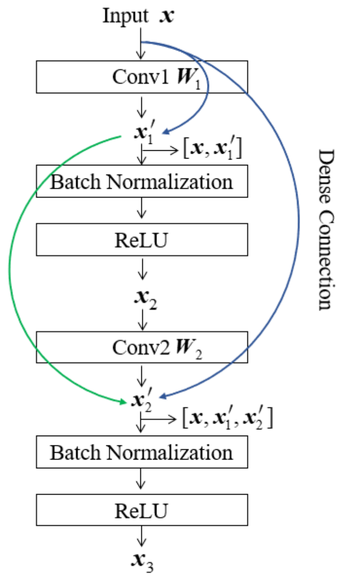
The overall architecture of DenseNet consists of alternating dense blocks and transition layers, where the dense block is the core unit for feature extraction. Different from traditional convolutional networks, where the input of each layer only comes from the output of the previous layer, in a dense block, the input of each convolutional layer includes not only the output of the previous layer, but also the output features of all preceding layers. A complete dense block is composed of several convolutional units, batch normalization layers, Leaky ReLU activation layers, and dense connections (green and blue curves), as illustrated in Figure 2.

For the $l$-th convolutional layer, its input ${\mathit{x}}_l$ contains the feature information of the initial input $\mathit{x}$, as well as the output features ${\mathit{x}}_1^{\prime },{\mathit{x}}_2^{\prime },\cdots ,{\mathit{x}}_{l-1}^{\prime }$ from the 1st to the $(l-1)$-th convolutional layers. Specifically, the outputs of all preceding layers are first concatenated along the channel dimension as $[\mathit{x},{\mathit{x}}_1^{\prime },{\mathit{x}}_2^{\prime },\cdots ,{\mathit{x}}_{l-1}^{\prime }]$, and then processed by batch normalization and the activation function to obtain the input of the $l$-th convolutional layer ${\mathit{x}}_l$, which is formulated as follows:

$${\mathit{x}}_l=\sigma (BN([\mathit{x},{\mathit{x}}_1^{\prime },{\mathit{x}}_2^{\prime },\cdots ,{\mathit{x}}_{l-1}^{\prime }]))$$

(4)

In Equation (4), $BN(\cdot )$ denotes the batch normalization operation, $\sigma (\cdot )$ represents the Leaky ReLU activation function, and $\sigma (\cdot )$ refers to feature concatenation along the channel dimension. In Figure 2, the express of ${\mathit{x}}_3$ is as follows:

$${\mathit{x}}_3=\sigma (BN([\mathit{x},{\mathit{x}}_1^{\prime },{\mathit{x}}_2^{\prime }]))$$

(5)

In Equation (5), $[\mathit{x},{\mathit{x}}_1^{\prime },{\mathit{x}}_2^{\prime }]$ denotes the feature concatenation of the initial input $\mathit{x}$, the output ${\mathit{x}}_1^{\prime }$ of convolutional layer ${\mathit{W}}_1$, and the output ${\mathit{x}}_2^{\prime }$ of convolutional layer ${\mathit{W}}_2$ along the channel dimension.

Nevertheless, such a concatenation mechanism leads to the continuous accumulation of feature channels after each convolutional layer, which greatly increases the computational complexity of the network. To address this issue, DenseNet introduces bottleneck layers and transition layers to reduce the computational cost of each convolutional layer.

Compared with residual connection, dense connection improves feature reuse through feature concatenation. However, it also substantially increases the network width and computational overhead, which may cause greater optimization difficulties when it is applied to deep temporal networks. Therefore, this study selects residual connection as the core enhancement mechanism for constructing deep temporal networks, and takes dense connection as the comparison mechanism, which will be elaborated via ablation comparison models in Section 2.4.

2.2. Gated Recurrent Unit

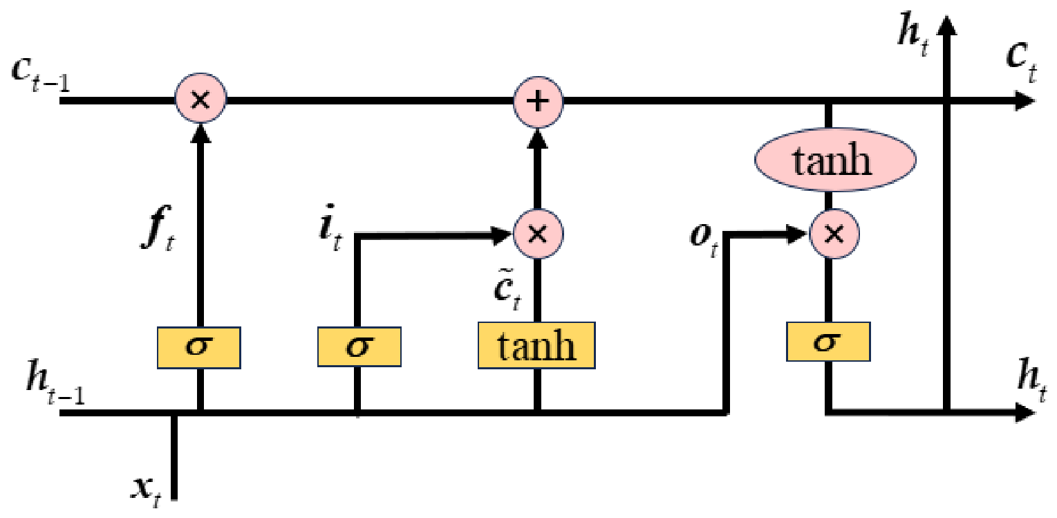
GRU is a lightweight variant of LSTM. It improves the hidden state updating mechanism of traditional recurrent neural networks by introducing the reset gate and the update gate. Compared with LSTM, GRU integrates the functions of the input gate, forget gate, and output gate in LSTM, and realizes the control of information flow with a more compact architecture. Specifically, GRU no longer maintains an independent cell state; instead, it merges the cell state with the hidden state and removes the output gate structure. It only relies on the update gate and reset gate to implement information filtering and transmission. In this way, GRU reduces model complexity while still being capable of effectively capturing temporal dependencies in sequence data. Its structure is illustrated in Figure 3.

At time step $t$, the inputs are the current input vector ${\mathit{x}}_t\in {ℝ}^d$ and the hidden state from the previous time step ${\mathit{h}}_{t-1}\in {ℝ}^m$, and the information update is completed through the following gating mechanism.

(1) Update Gate: It controls the degree of influence of the previous hidden state ${\mathit{h}}_{t-1}$ on the current hidden state ${\mathit{h}}_t$. The update gate takes the current input ${\mathit{x}}_t$ and the previous hidden state ${\mathit{h}}_{t-1}$ as inputs, and maps the values to the interval $(0,1)$ via the Sigmoid activation function. An output value closer to 1 means that more historical information is retained, while a value closer to 0 indicates that more current input information is adopted. The specific calculation formula is given as follows:

$${\mathit{z}}_t=\sigma ({\mathit{W}}_z{\mathit{x}}_t+{\mathit{U}}_z{\mathit{h}}_{t-1}+{\mathit{b}}_z)$$

(6)

In Equation (6), ${\mathit{z}}_t$ denotes the output of the update gate, ${\mathit{W}}_z$ and ${\mathit{U}}_z$ are the weight matrices of the update gate, ${\mathit{b}}_z$ is the update gate bias, and $\sigma (\cdot )$ refers to the Sigmoid activation function.

(2) Reset Gate: It controls the degree to which the previous time step hidden state ${\mathit{h}}_{t-1}$ influences the candidate hidden state ${\tilde{\mathit{h}}}_t$ at the current time step. Its output value ${\mathit{r}}_t$ is also mapped to the interval $(0,1)$. When ${\mathit{r}}_t$ is closer to 0, less information from the previous hidden state ${\mathit{h}}_{t-1}$ is retained, so the model pays more attention to the current input information. The specific calculation formula is expressed as follows:

$${\mathit{r}}_t=\sigma ({\mathit{W}}_r{\mathit{x}}_t+{\mathit{U}}_r{\mathit{h}}_{t-1}+{\mathit{b}}_r)$$

(7)

In Equation (7), ${\mathit{W}}_r$ and ${\mathit{U}}_r$ denote the weight matrices of the reset gate, ${\mathit{b}}_r$ is the bias of the reset gate, and $\sigma (\cdot )$ represents the Sigmoid activation function.

(3) Candidate Hidden State: It integrates the current input and the previous hidden state ${\mathit{h}}_{t-1}$ filtered by the reset gate ${\mathit{r}}_t$ to generate the candidate hidden state ${\tilde{\mathit{h}}}_t$ at the current time step. When generating the candidate hidden state ${\tilde{\mathit{h}}}_t$, the reset gate is utilized to filter the previous hidden state ${\mathit{h}}_{t-1}$, suppress the interference of irrelevant historical information, and enable the model to focus more on the current input features. The specific calculation formula is given as follows:

$${\tilde{\mathit{h}}}_t=\tanh ({\mathit{W}}_h{\mathit{x}}_t+{\mathit{U}}_h(r_t\odot {\mathit{h}}_{t-1})+{\mathit{b}}_h)$$

(8)

In Equation (8), ${\mathit{W}}_h$ and ${\mathit{U}}_h$ are the weight matrices of the candidate hidden state, ${\mathit{b}}_h$ denotes the bias of the candidate hidden state, $\tanh (\cdot )$ is the activation function, and $\odot$ represents the element-wise Hadamard product.

(4) Hidden State Update: The final hidden state ${\mathit{h}}_t$ of the GRU is obtained as a weighted combination of the previous hidden state ${\mathit{h}}_{t-1}$ and the candidate hidden state ${\tilde{\mathit{h}}}_t$, with the weights of both components controlled by the output ${\mathit{z}}_t$ of the update gate. The calculation formula is expressed as follows:

$${\mathit{h}}_t=(1-{\mathit{z}}_t)\odot {\mathit{h}}_{t-1}+{\mathit{z}}_t\odot {\tilde{\mathit{h}}}_t$$

(9)

In Equation (9), $\odot$ denotes element-wise multiplication. The term ${\mathit{z}}_t\odot {\tilde{\mathit{h}}}_t$ represents the selective update of the current candidate hidden state ${\tilde{\mathit{h}}}_t$, while the term $(1-{\mathit{z}}_t)\odot {\mathit{h}}_{t-1}$ indicates the degree of information retention from the previous time step hidden state ${\mathit{h}}_{t-1}$.

In this study, the GRU with a more concise structure is selected as the basic unit for constructing the deep temporal network. Meanwhile, LSTM is adopted as the comparative recurrent unit, and relevant ablation and comparative model analysis are presented in Section 2.4.

2.3. Residual GRU Model

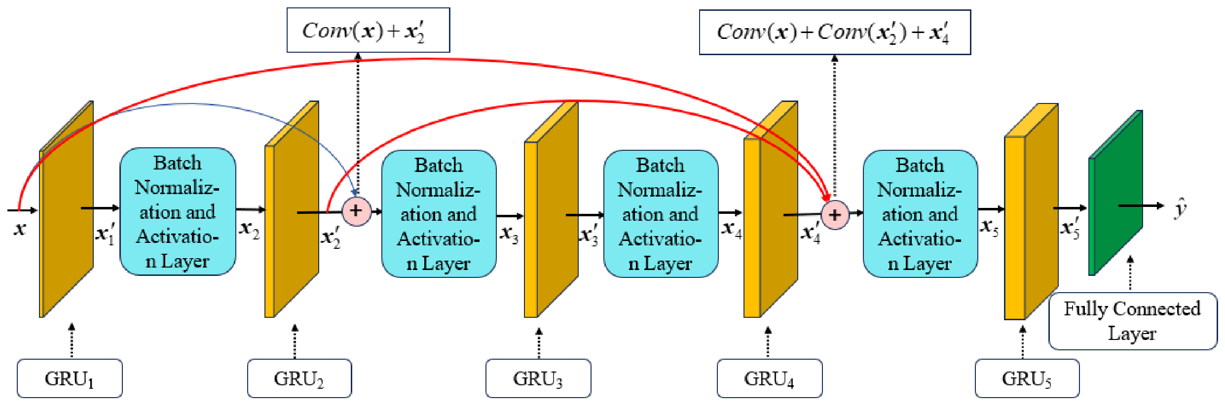
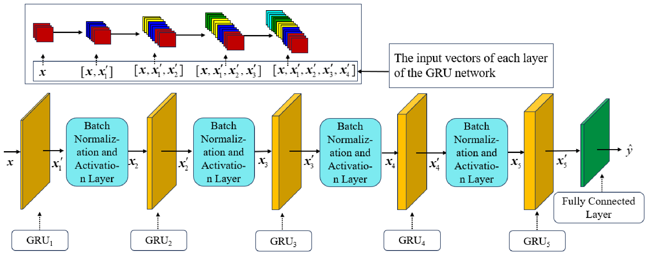
Based on the design concept of the residual block described in Section 2.1.1, this study combines residual connections with the GRU to construct a recurrent neural network model named RGRU with residual paths, to improve the model’s stability and feature representation capability when processing high-dimensional time-series financial data. Specifically, according to the residual structure shown in Figure 1, all convolutional layers in the residual unit are replaced with GRUs, and a five-layer RGRU model is constructed. The overall architecture of the proposed model is illustrated in Figure 4.

According to the RGRU model illustrated in Figure 4, the constructed residual connection network consists of five deep neural network layers and one fully connected layer. There are two residual paths in the overall network: one is arranged between the second and the third layer, and the other is arranged between the fourth and the fifth layer. To unify the feature dimensions and reduce the risk of overfitting in the case of a limited sample size, we inserted batch normalization layers, Leaky ReLU activation layers, and Dropout regularization modules between each adjacent layer. The embedded batch normalization, Leaky ReLU activation function, and Dropout regularization module combine two residual skip paths to jointly constrain the effective capacity of the five-layer-deep recurrent network. This composite architecture significantly alleviates the problems caused by the limited sample size, including the inherent gradient disappearance problem of stacked deep GRU layers and the overfitting problem of noise and outliers in small-scale financial datasets, thereby stabilizing the model convergence and improving the generalization ability of enterprise financial time-series prediction. The specific forward propagation process is described below.

(1) After receiving the initial input $\mathit{x}$, the network extracts hidden features through the first deep recurrent layer ${\mathrm{GRU}}_1$ and generates the output ${\mathit{x}}_1^{\prime }$, and the formula is expressed as follows:

$${\mathit{x}}_1^{\prime }={\mathrm{GRU}}_1(\mathit{x})$$

(10)

In Equation (10), ${\mathrm{GRU}}_1(\cdot )$ denotes the first recurrent neural network unit ${\mathrm{GRU}}_1$.

(2) To improve the training stability and generalization ability of the model, the extracted features are processed with batch normalization, Leaky ReLU activation, and Dropout regularization, to obtain the input ${\mathit{x}}_2$ of the second neural network layer. The corresponding formulas are given as follows:

$${\mathit{x}}_2^{bn}=BN({\mathit{x}}_1^{\prime })$$

(11)

$${\mathit{x}}_2^{act}=\sigma ({\mathit{x}}_2^{bn})$$

(12)

$${\mathit{x}}_2^{out}=D({\mathit{x}}_2^{act})$$

(13)

$${\mathit{x}}_2={\mathit{x}}_2^{out}$$

(14)

In Equations (11)–(14), $BN(\cdot )$ represents the batch normalization operation, $\sigma (\cdot )$ denotes the Leaky ReLU activation function, and $D(\cdot )$ refers to the Dropout regularization operation. ${\mathit{x}}_2^{bn}$ is the output after batch normalization, ${\mathit{x}}_2^{act}$ is the output of the activation function, and ${\mathit{x}}_2^{out}$ is the output after regularization. Subsequently, the second neural network layer ${\mathrm{GRU}}_2$ further extracts hidden features, and the final output is obtained as ${\mathit{x}}_2^{\prime }={\mathrm{GRU}}_2({\mathit{x}}_2)$.

(3) Based on the idea of residual connection, the initial input $\mathit{x}$ and the output of the previous layer ${\mathit{x}}_2^{\prime }$ are summed to realize the deep fusion of features. Because the dimensions of the initial input $\mathit{x}$ and the previous layer output ${\mathit{x}}_2^{\prime }$ are inconsistent, this study adopts a $1\times 1$ convolution operation to project the initial input $\mathit{x}$ into the same dimension as ${\mathit{x}}_2^{\prime }$; the new feature representation ${\mathit{x}}_2^{″}$ can be obtained.

$${\mathit{x}}_2^{″}={\mathit{W}}_s^1\mathit{x}+{\mathit{x}}_2^{\prime }$$

(15)

In Equation (15), ${\mathit{W}}_s^1$ represents the weight matrix of a $1\times 1$ convolution; at this point, the dimensions of ${\mathit{W}}_s^1\mathit{x}$ and ${\mathit{x}}_2^{\prime }$ are the same.

After the summation operation is completed, in order to enhance the training stability and generalization ability of the model, it is necessary to sequentially perform batch normalization processing, Leaky ReLU activation, and Dropout regularization operations on it, obtaining the input ${\mathit{x}}_3$ of the third-layer neural network ${\mathrm{GRU}}_3$. The calculation process can be expressed as follows:

$${\mathit{x}}_3=D(\sigma (BN({\mathit{x}}_2^{″})))$$

(16)

Subsequently, ${\mathrm{GRU}}_3$ is utilized for further deep feature extraction to generate the output ${\mathit{x}}_3^{\prime }$.

(4) For the fourth recurrent neural network layer ${\mathrm{GRU}}_4$, its input ${\mathit{x}}_4$ is obtained by processing the output ${\mathit{x}}_3^{\prime }$ through batch normalization, ReLU activation, and Dropout regularization operations.

(5) Finally, the initial input $\mathit{x}$, the previous layer output ${\mathit{x}}_2^{\prime }$, and ${\mathit{x}}_4^{\prime }$ are summed together, and the new feature representation ${\mathit{x}}_4^{″}$ can be obtained. After feature transformation and regularization processing, the result ${\mathit{x}}_5$ is fed into the fifth recurrent neural network layer ${\mathrm{GRU}}_5$, and the output ${\mathit{x}}_5^{\prime }$ can be obtained to extract richer and hierarchical feature information. Its calculation process can be expressed as follows:

$${\mathit{x}}_4^{″}={\mathit{W}}_s^2\mathit{x}+{\mathit{W}}_s^3{\mathit{x}}_2^{\prime }+{\mathit{x}}_4^{\prime }$$

(17)

$${\mathit{x}}_5=D(\sigma (BN({\mathit{x}}_4^{″})))$$

(18)

$${\mathit{x}}_5^{\prime }={\mathrm{GRU}}_5({\mathit{x}}_5)$$

(19)

In Equation (17), ${\mathit{W}}_s^2$ and ${\mathit{W}}_s^3$ are the weight matrices of different $1\times 1$ convolutions.

(6) Ultimately, ${\mathit{x}}_5^{\prime }$ is mapped to the prediction output layer through the fully connected layer to obtain the class score vector $\mathit{z}$, which is expressed as follows:

$$\mathit{z}=\mathit{V}{\mathit{x}}_5^{\prime }+\mathit{b}$$

(20)

In Equation (20), $\mathit{V}$ denotes the weight matrix of the fully connected layer, and $\mathit{b}$ represents the bias term of the fully connected layer.

2.4. Ablation Comparison Model

2.4.1. Residual LSTM Model

To verify the effectiveness of introducing residual connections, this study also constructs the RLSTM model for isomorphic comparison with the proposed RGRU model. Specifically, under the identical residual connection architecture and network depth, the basic recurrent unit GRU is replaced with LSTM. With this design, under the same residual connection mechanism, the time-series modeling performance based on different recurrent units can be fairly compared. In detail, in the established RGRU architecture, the GRU at each layer is substituted with an LSTM unit. For instance, in the RGRU model, the hidden features extracted and output by the $l$-th recurrent unit can be formulated as follows:

$${\mathit{x}}_l^{\prime }={\mathrm{GRU}}_l({\mathit{x}}_l)$$

(21)

Correspondingly, the output of the $l$-th recurrent unit in the RLSTM model is expressed as follows:

$${\mathit{x}}_l^{\prime }={\mathrm{LSTM}}_l({\mathit{x}}_l)$$

(22)

Apart from the difference in the basic recurrent unit, the residual fusion addition operation, batch normalization processing, Leaky ReLU activation function, and Dropout regularization operation are kept completely consistent between the RGRU and RLSTM models.

2.4.2. Dense GRU Model and Dense LSTM Model

To systematically evaluate the influence of the residual connection mechanism on the early-warning model, this study further conducts ablation comparison with dense connection architecture. Specifically, on the premise of controlling the type of basic recurrent unit, the residual connections are replaced with dense connections, and two comparative models, namely DGRU and DLSTM, are constructed simultaneously. Specifically, according to the dense structure illustrated in Figure 2 of Section 2.1.2, all convolutional layers in the dense block are replaced with GRU or LSTM units. Meanwhile, through feature concatenation operation, the initial input and the outputs of all previous layers are jointly transmitted to subsequent layers, so that shallow and deep features can be fully fused. The DGRU model is presented in Figure 5.

As illustrated in Figure 5, the overall DGRU model also consists of five recurrent neural network layers and one fully connected output layer. The input of each layer follows the dense connection concatenation rule of “initial input + outputs of all previous layers.” Meanwhile, before feeding the concatenated fused features into each GRU layer, the same feature transformation and regularization modules as those in the residual fusion model are introduced. The forward propagation process of the model is described as follows:

(1) After receiving the initial input $\mathit{x}$, the network first performs preliminary hidden feature extraction through the first recurrent layer ${\mathrm{GRU}}_1$ and generates the output ${\mathit{x}}_1^{\prime }$, which is defined as follows:

$${\mathit{x}}_1^{\prime }={\mathrm{GRU}}_1(\mathit{x})$$

(23)

In Equation (23), ${\mathrm{GRU}}_1(\cdot )$ denotes the first neural network unit ${\mathrm{GRU}}_1$.

(2) The input of the second neural network layer does not directly adopt the output of the previous layer; it concatenates the initial input $\mathit{x}$ and the output ${\mathit{x}}_1^{\prime }$ of the first layer ${\mathrm{GRU}}_1$ along the feature channel dimension to construct the fused feature $[\mathit{x},{\mathit{x}}_1^{\prime }]$. Subsequently, batch normalization, Leaky ReLU activation, and regularization operations are performed sequentially to obtain the input ${\mathit{x}}_2$ of the second recurrent layer ${\mathrm{GRU}}_2$. The corresponding formulas are given as follows:

$${\mathit{u}}_2=[\mathit{x},{\mathit{x}}_1^{\prime }]$$

(24)

$${\mathit{x}}_2^{bn}=BN({\mathit{u}}_2)$$

(25)

$${\mathit{x}}_2^{act}=\sigma ({\mathit{x}}_2^{bn})$$

(26)

$${\mathit{x}}_2^{out}=D({\mathit{x}}_2^{act})$$

(27)

$${\mathit{x}}_2={\mathit{x}}_2^{out}$$

(28)

In Equations (24)–(28), ${\mathit{u}}_2$ denotes the feature vector obtained by concatenating the initial input and the first layer output, $[\cdot ]$ represents feature concatenation along the channel dimension, $BN(\cdot )$ denotes the batch normalization operation, $\sigma (\cdot )$ represents the Leaky ReLU activation function, and $D(\cdot )$ refers to the Dropout regularization operation. ${\mathit{x}}_2^{bn}$ is the output after batch normalization, ${\mathit{x}}_2^{act}$ is the output of the activation function, and ${\mathit{x}}_2^{out}$ is the output after regularization.

(3) For the subsequent recurrent neural network layers ${\mathrm{GRU}}_3$, ${\mathrm{GRU}}_4$, and ${\mathrm{GRU}}_5$, the same dense connection construction method is adopted. The input of each layer is formed by concatenating the initial input $\mathit{x}$ with the outputs of all previous network layers, to construct a fused representation of multi-layer features.

As the network depth increases, the feature dimension fed into each layer gradually expands. Meanwhile, the dimension of concatenated features keeps growing, enabling the model to directly retain and extract shallow basic features, thus realizing lossless and efficient information flow across network layers. The corresponding formulas are expressed as follows:

$${\mathit{u}}_3=[\mathit{x},{\mathit{x}}_1^{\prime },{\mathit{x}}_2^{\prime }]$$

(29)

$${\mathit{u}}_4=[\mathit{x},{\mathit{x}}_1^{\prime },{\mathit{x}}_2^{\prime },{\mathit{x}}_3^{\prime }]$$

(30)

$${\mathit{u}}_5=[\mathit{x},{\mathit{x}}_1^{\prime },{\mathit{x}}_2^{\prime },{\mathit{x}}_3^{\prime },{\mathit{x}}_4^{\prime }]$$

(31)

In Equations (29)–(31), ${\mathit{u}}_3$ denotes the feature vector obtained by concatenating the initial input with the outputs of the first and second layers, ${\mathit{u}}_4$ represents the feature vector formed by concatenating the initial input with the outputs of the first three layers, and ${\mathit{u}}_5$ refers to the feature vector generated by concatenating the initial input with the outputs of the first four layers.

(4) Meanwhile, before the input of each layer, batch normalization, Leaky ReLU activation function, and Dropout regularization operations are performed, which can alleviate the risk of gradient vanishing and enhance the model’s capability to fit complex nonlinear patterns. The formulas are expressed as follows:

$${\mathit{x}}_k^{bn}=BN({\mathit{u}}_k)$$

(32)

$${\mathit{x}}_k^{act}=\sigma ({\mathit{x}}_k^{bn})$$

(33)

$${\mathit{x}}_k^{out}=D({\mathit{x}}_k^{act})$$

(34)

In Equations (32)–(34), ${\mathit{u}}_k,k=3,4,5$ represents the $k$-th layer concatenation vector; ${\mathit{x}}_k^{bn},k=3,4,5$ represents the output of batch normalization before feeding into the $k$-th layer; ${\mathit{x}}_k^{act},k=3,4,5$ refers to the activation output before the $k$-th layer input; and ${\mathit{x}}_k^{out},k=3,4,5$ indicates the regularization output prior to the $k$-th layer input.

Accordingly, the input of each layer can be obtained sequentially as follows:

$${\mathit{x}}_3={\mathit{x}}_3^{out}$$

(35)

$${\mathit{x}}_4={\mathit{x}}_4^{out}$$

(36)

$${\mathit{x}}_5={\mathit{x}}_5^{out}$$

(37)

In Equations (35)–(37), ${\mathit{x}}_3$, ${\mathit{x}}_4$, and ${\mathit{x}}_5$ are the inputs of ${\mathrm{GRU}}_3$, ${\mathrm{GRU}}_4$, and ${\mathrm{GRU}}_5$, respectively, and ${\mathit{x}}_3^{out}$, ${\mathit{x}}_4^{out}$, and ${\mathit{x}}_5^{out}$ are the corresponding regularization outputs of each layer.

(5) After the feature extraction of the five-layer recurrent neural network, the model performs the final concatenation of the initial input and the outputs of all five layers along the feature channel dimension to construct the input vector ${\mathit{x}}_{input}$ of the fully connected layer, which is expressed as follows:

$${\mathit{x}}_{input}=[\mathit{x},{\mathit{x}}_1^{\prime },{\mathit{x}}_2^{\prime },{\mathit{x}}_3^{\prime },{\mathit{x}}_4^{\prime },{\mathit{x}}_5^{\prime }]$$

(38)

(6) Finally, the input ${\mathit{x}}_{input}$ is mapped to the output layer via linear transformation to obtain the class score vector $\mathit{z}$; namely, the following:

$$\mathit{z}=\mathit{V}{\mathit{x}}_{input}+\mathit{b}$$

(39)

In Equation (39), $\mathit{V}$ denotes the weight matrix of the fully connected layer and $\mathit{b}$ represents the bias term of the fully connected layer.

For the DLSTM model, the recurrent unit at each layer of the DGRU is replaced with an LSTM unit. Meanwhile, the batch normalization processing, Leaky ReLU activation function, and Dropout regularization operations between each layer are exactly the same as those in the DGRU model.

3. Construction of the Early-Warning Indicator System and Data Processing

3.1. Data Sources and Sample Selection

The financial data, the Special Treatment (ST) or Delisting Risk Warning (*ST) status labels of listed companies, the industry classification information, and the corporate governance data used in this study are all obtained from the China Stock Market & Accounting Research (CSMAR) database [23]. This database provides comprehensive financial indicators, market transaction records, and governance information for listed Chinese firms.

This study selects the quarterly data of A-share listed companies from the first quarter of 2010 to the fourth quarter of 2024 as the research sample. Companies in financial distress are defined as those marked as ST or *ST by the stock exchange. The date of the risk warning announcement is defined as period $t$. Data from the past are selected to construct a continuous financial data observation window from $t-1$ to $t-8$ quarters. If the same company triggers multiple warnings at different times, all samples corresponding to each time window of that company will be retained to capture dynamic risks and expand the effective sample size. In the subsequent data division, potential correlations will be controlled. Meanwhile, the influence of industry differences and scale effects is eliminated, and each distress company is matched with an equally sized and industry-aligned non-distress company on a 1:1 basis.

3.2. Selection of Early-Warning Characteristic Indicators

In line with the research objective of financial distress prediction, this study systematically explores the characteristics of financial risks, synthesizes the theoretical achievements of existing literature in the screening of financial early-warning indicators, and constructs an evaluation system incorporating 47 financial and non-financial early-warning indicators [24]. Among them, the financial indicators cover seven dimensions—debt repayment ability, operational ability, profitability, cost and expense structure, cash flow ability, development ability, per-share indicators, and market performance—to comprehensively assess the financial and operational risks of the enterprise. At the same time, factors such as equity concentration, the proportion of independent directors, the proportion of management’s holdings, the number of company executives, the type of audit opinion, and the total number of companies in the industry have all been included in the early-warning indicator system as non-financial characteristic indicators to comprehensively reflect the equity structure, governance level, management incentive mechanism, external audit constraints, and industry competition situation of the enterprise. Specific indicators are detailed in

Table 1. Financial index system.

First-Level Indicators	Second-Level Indicators
Solvency	Current ratio, quick ratio, cash ratio, cash flow to current liabilities ratio, asset–liability ratio, interest coverage ratio, equity ratio, equity-to-asset ratio, total long-term liabilities, operating liability ratio, equity to fixed assets ratio
Operational capacity	Inventory turnover ratio, total asset turnover ratio, capital intensity, tangible asset ratio, current asset ratio
Profitability	Total asset net profit margin, return on assets, return on net assets, return on invested capital, return on investment, operating cost ratio, net operating profit margin, net profit attributable to shareholders of listed companies excluding non-recurring gains and losses
Expense and cost structure	Financial expense ratio, R&D expense ratio, turnover tax rate, comprehensive tax rate
Cash flow capacity	Operating index, net cash content of net profit, growth rate of net cash flow from investing activities, growth rate of net cash flow from financing activities
Development capability	Growth rate of selling expenses, growth rate of operating revenue, capital accumulation rate, growth rate of total assets
Per-share indicators and market performance	Earnings per share, depreciation and amortization per share, net assets per share, operating profit per share, price-to-earnings ratio
Non-financial indicators	Shareholding ratio of the largest shareholder, proportion of independent directors, shareholding ratio of management, number of senior executives, types of audit opinions, total number of companies in the industry

.

All the indicators are derived from the CSMAR database and are traditional financial and corporate governance indicators with unified calculation standards. The specific definition standards for the four indicators of operating index, capital intensity, types of audit opinions, and total number of companies in the industry are as follows:

(1)

Operating index: Calculated as net cash flow from operating activities divided by operating profit. This indicator quantifies the cash support strength of book profits and evaluates the real earnings quality of listed firms.

(2)

Capital intensity: Defined as net fixed assets/operating revenue. It measures the degree of asset heaviness; a higher value means more fixed asset investment is required to generate unit operating income.

(3)

Types of audit opinions: A dummy variable. Based on the standard scoring system of the Guotai Nan Database, the scores are as follows: a standard unqualified opinion is assigned a score of 1, a qualified opinion is assigned a score of 2, a negative opinion is assigned a score of 3, an opinion that cannot be expressed is assigned a score of 4, an unqualified opinion with explanatory remarks is assigned a score of 5, and a qualified opinion with an item section is assigned a score of 6.

(4)

Total number of companies in the industry: Represents the total quantity of A-share listed enterprises within the corresponding primary Shenwan (SW) industry in each sample year, adopted to control cross-sectional industry heterogeneity in regression analysis.

3.3. Data Processing

Due to the diverse sources of enterprise financial data, the long-time span, and the different disclosure environments, the original data exhibit differences in terms of completeness and consistency. If directly used for model training, it may lead to unbalanced sample distribution and variable distribution imbalance, thereby affecting the interpretability and reliability of the prediction results. Therefore, in this section, starting from data quality control, we focus on elaborating on the methods for handling missing values and data standardization to ensure that the subsequent model analysis is based on stable and well-structured data.

All the data processing, model construction, and result visualization in this study were implemented using Python 3.12. This software is developed and maintained by the Python Software Foundation (PSF), with its official address at Beaverton, OR, USA. The data processing involved in the above process and the related scripts are all stored in the Supplementary Materials (Supplementary Folder S1).

3.3.1. Handling of Missing Values

This study obtains quarterly characteristic indicator data of Chinese A-share listed enterprises from the CSMAR database covering the period from 2010 to 2024. According to the forward rolling extraction of eight-quarter data described in Section 3.1, all samples corresponding to each time window are retained and, finally, 1710 financially distressed enterprise samples are obtained. After matching the distressed sample with normal enterprises in a 1:1 ratio, an initial paired sample set consisting of 1710 distressed enterprise samples and 1710 normal enterprise samples was formed.

During the data preprocessing stage, the missing values in all paired distressed enterprises and normal enterprises are first handled. The overall missing rate is then calculated based on the total number of data points. Each individual enterprise has a total of 376 data points, and the overall missing rate is defined as the proportion of missing values among all expanded data points of the enterprise. Enterprises with an overall missing rate of financial data exceeding 20% are considered to suffer from severe discontinuity in information disclosure and cannot meet the basic requirements of subsequent time-series modeling. Therefore, such paired samples are entirely eliminated: if either the distressed enterprise or its matched normal enterprise in a sample pair has a missing rate higher than 20%, the whole sample pair is removed. This processing strategy maintains the original matching relationship and sample balance, while effectively mitigating systematic bias caused by large-scale missing data. After the above screening process, 1286 valid financially distressed enterprise samples and the corresponding 1286 matched normal enterprise samples are finally retained, constructing a balanced dataset with a total of 2572 enterprise observations.

For the remaining missing values of each indicator across the 2572 retained enterprises, this study adopts the historical mean imputation within the enterprise and feature to fill the gaps. The mathematical formula is expressed as follows:

$${\widehat{x}}_{q,j}^{(p)}={\displaystyle \frac{1}{T}}{\displaystyle \sum _{r=1}^T{x}_{r,j}^{(p)}}$$

(40)

In Equation (40), $x_{r,j}^{(p)},r=t-8,t-7,\cdots ,t-1,j=1,2,\cdots ,47,p=1,2,\cdots ,2572$ denotes the original observed value of the $r$-th time step for the $j$-th feature indicator of the $p$-th enterprise, ${\widehat{x}}_{q,j}^{(p)}$ refers to the imputed result of the missing value at the $q$-th time step for the $j$-th feature indicator of the $p$-th enterprise, and $T$ represents the number of actual observation periods.

While maintaining the stability of individual enterprise characteristics, this method avoids the structural bias that may be introduced by cross-enterprise imputation, and can effectively preserve the consistency of variable dimensions as well as the comparability of research samples. The sample data are consistent in the input structure of each model.

3.3.2. Descriptive Statistical Analysis

To provide an overall understanding of the sample characteristics, descriptive statistical analyses were conducted for all variables included in the study. The statistics were computed separately for distressed and non-distressed firms. Due to space limitations, representative descriptive statistics are reported in

Table 2. Descriptive statistics of some indicators for distressed firms.

Indicator	Mean	Standard Deviation	Minimum	Maximum	Lower Quartile	Upper Quartile
Current ratio	2.21	19.48	0.01	1883.35	0.66	1.78
Quick ratio	1.66	7.71	0.00	666.24	0.41	1.32
Cash ratio	0.50	2.41	−0.16	144.12	0.03	0.32
Cash flow to current liabilities ratio	−0.04	1.77	−171.67	21.53	−0.08	0.04
Asset–liability ratio	0.64	0.48	0.00	12.70	0.40	0.84
Interest coverage ratio	−52.20	1322.47	−37,717.19	46,273.48	−6.99	1.28
Equity ratio	4.46	159.31	−8740.36	11,125.03	0.43	3.25
Equity-to-asset ratio	0.30	0.98	−63.10	0.99	0.11	0.57
Total long-term liabilities	1.30 × 109	4.45 × 109	0.00	1.00 × 1011	1.55 × 107	1.13 × 109
Operating liability ratio	0.52	0.24	−0.04	1.00	0.33	0.70
Equity-to-fixed-assets ratio	111.54	1778.81	−10,497.20	65,029.04	0.75	7.50
Inventory turnover ratio	456.28	14,356.24	0.00	916,542.12	0.62	5.46

and

Table 3. Descriptive statistics of some indicators for non-distressed firms.

Indicator	Mean	Standard Deviation	Minimum	Maximum	Lower Quartile	Upper Quartile
Current ratio	3.58	5.30	−23.73	160.95	1.31	3.79
Quick ratio	2.95	5.00	−20.08	153.14	0.86	3.07
Cash ratio	1.29	3.06	−17.73	104.19	0.21	1.21
Cash flow to current liabilities ratio	0.09	0.49	−7.63	6.66	−0.06	0.20
Asset–liability ratio	0.38	0.24	−0.09	6.28	0.20	0.53
Interest coverage ratio	86.77	1108.65	−4056.84	85,380.59	2.23	46.56
Equity ratio	1.16	25.81	−493.90	2541.05	0.24	1.10
Equity-to-asset ratio	0.61	0.25	−5.28	0.99	0.47	0.79
Total long-term liabilities	1.85 × 109	8.26 × 109	−5.35 × 109	1.39 × 1011	7.64 × 106	1.28 × 109
Operating liability ratio	0.59	0.26	−0.81	1.00	0.38	0.82
Equity-to-fixed-assets ratio	18.58	92.79	−4024.72	2459.74	2.16	9.82
Inventory turnover ratio	138.96	2768.57	−0.09	107,130.89	0.68	4.26

, while the complete set of results is presented in

Table A1. Descriptive statistics of all indicators for distressed firms.

Indicator	Mean	Standard Deviation	Minimum	Maximum	Lower Quartile	Upper Quartile
Current ratio	2.21	19.48	0.01	1883.35	0.66	1.78
Quick ratio	1.66	7.71	0.00	666.24	0.41	1.32
Cash ratio	0.50	2.41	−0.16	144.12	0.03	0.32
Cash flow to current liabilities ratio	−0.04	1.77	−171.67	21.53	−0.08	0.04
Asset–liability ratio	0.64	0.48	0.00	12.70	0.40	0.84
Interest coverage ratio	−52.20	1322.47	−37,717.19	46,273.48	−6.99	1.28
Equity ratio	4.46	159.31	−8740.36	11,125.03	0.43	3.25
Equity-to-asset ratio	0.30	0.98	−63.10	0.99	0.11	0.57
Total long-term liabilities	1.30 × 109	4.45 × 109	0.00	1.00 × 1011	1.55 × 107	1.13 × 109
Operating liability ratio	0.52	0.24	−0.04	1.00	0.33	0.70
Equity-to-fixed-assets ratio	111.54	1778.81	−10,497.20	65,029.04	0.75	7.50
Inventory turnover ratio	456.28	14,356.24	0.00	916,542.12	0.62	5.46
Total asset turnover ratio	0.26	0.41	−0.06	11.60	0.07	0.32
Capital intensity	248.11	13,396.00	0.09	984,913.33	3.11	14.24
Tangible asset ratio	0.92	0.11	0.23	1.00	0.90	0.98
Current asset ratio	0.51	0.22	0.00	1.00	0.35	0.67
Total asset net profit margin	−0.05	0.23	−7.70	7.45	−0.05	0.00
Return on assets	−0.04	0.23	−7.16	9.35	−0.04	0.01
Return on net assets	−0.21	12.35	−186.56	281.99	−0.21	0.01
Return on invested capital	−0.09	0.73	−41.17	22.01	−0.06	0.01
Return on investment	−8.32	890.58	−61,023.49	25,488.73	−0.04	0.04
Operating cost ratio	0.82	0.56	−0.04	45.06	0.70	0.93
Net operating profit margin	−3.46	140.97	−10,243.95	24.25	−0.41	0.01
Net profit attributable to shareholders of listed companies excluding non-recurring gains and losses	−2.79 × 108	1.59 × 109	−5.57 × 1010	4.03 × 109	−1.54 × 108	−1.35 × 106
Financial expense ratio	0.34	13.06	−45.75	1294.70	0.01	0.11
R&D expense ratio	0.08	0.20	0.00	7.64	0.03	0.08
Turnover tax rate	0.02	0.18	−9.47	12.49	0.00	0.02
Comprehensive tax rate	0.02	0.65	−59.85	12.49	0.00	0.03
Operating index	2.29	265.09	−2823.65	25,037.97	−0.66	1.34
Net cash content of net profit	−1.08	75.86	−3538.09	2392.92	−1.13	1.34
Growth rate of net cash flow from investing activities	10,589.12	5.67 × 105	−8.72 × 105	5.43 × 107	−1.99	2.48
Growth rate of net cash flow from financing activities	0.17	161.13	−4822.68	13,055.30	−2.01	0.58
Growth rate of selling expenses	19.52	654.22	−1.06	40,671.29	−0.31	0.19
Growth rate of operating revenue	2.26	96.12	−29.48	9290.91	−0.29	0.27
Capital accumulation rate	−0.53	6.58	−190.38	76.90	−0.20	0.01
Growth rate of total assets	−0.01	0.33	−0.97	10.35	−0.08	0.02
Earnings per share	−0.25	0.86	−24.46	10.29	−0.25	0.01
Depreciation and amortization per share	0.07	0.17	−0.10	6.93	0.00	0.07
Net assets per share	2.43	3.01	−11.41	43.06	0.64	3.42
Operating profit per share	−0.23	0.85	−23.95	10.35	−0.24	0.01
Price-to-earnings ratio	35.76	416.51	0.10	20,452.06	1.82	8.94
The shareholding ratio of the largest shareholder (%)	26.98	13.25	2.23	76.22	17.15	33.45
Proportion of independent directors (%)	38.47	6.01	25.00	75.00	33.33	42.86
Shareholding ratio of management (%)	4.89	11.34	0.00	77.99	0.00	3.01
Number of senior executives	5.34	2.28	0.00	24.00	4.00	7.00
Types of audit opinions	2.70	1.84	1.00	6.00	1.00	5.00
Total number of companies in the industry	41.06	29.61	1.00	119.00	16.00	63.00

and

Table A2. Descriptive statistics of all indicators for non-distressed firms.

Indicator	Mean	Standard Deviation	Minimum	Maximum	Lower Quartile	Upper Quartile
Current ratio	3.58	5.30	−23.73	160.95	1.31	3.79
Quick ratio	2.95	5.00	−20.08	153.14	0.86	3.07
Cash ratio	1.29	3.06	−17.73	104.19	0.21	1.21
Cash flow to current liabilities ratio	0.09	0.49	−7.63	6.66	−0.06	0.20
Asset–liability ratio	0.38	0.24	−0.09	6.28	0.20	0.53
Interest coverage ratio	86.77	1108.65	−4056.84	85,380.59	2.23	46.56
Equity ratio	1.16	25.81	−493.90	2541.05	0.24	1.10
Equity-to-asset ratio	0.61	0.25	−5.28	0.99	0.47	0.79
Total long-term liabilities	1.85 × 109	8.26 × 109	−5.35 × 109	1.39 × 1011	7.64 × 106	1.28 × 109
Operating liability ratio	0.59	0.26	−0.81	1.00	0.38	0.82
Equity-to-fixed-assets ratio	18.58	92.79	−4024.72	2459.74	2.16	9.82
Inventory turnover ratio	138.96	2768.57	−0.09	107,130.89	0.68	4.26
Total asset turnover ratio	0.29	0.27	−0.13	4.83	0.11	0.39
Capital intensity	16.99	187.73	0.02	9678.74	2.58	9.43
Tangible asset ratio	0.93	0.09	0.18	1.00	0.91	0.98
Current asset ratio	0.58	0.21	0.03	0.99	0.43	0.74
Total asset net profit margin	0.02	0.06	−1.92	2.16	0.00	0.04
Return on assets	0.03	0.06	−1.84	2.26	0.01	0.05
Return on net assets	0.02	0.75	−66.45	7.81	0.01	0.06
Return on invested capital	0.03	0.13	−7.39	7.37	0.01	0.05
Return on investment	0.93	24.81	−1397.67	735.94	0.00	0.13
Operating cost ratio	0.69	0.23	−0.10	3.89	0.58	0.82
Net operating profit margin	−0.63	33.09	−2637.69	42.10	0.02	0.16
Net profit attributable to shareholders of listed companies excluding non-recurring gains and losses	7.78 × 107	5.36 × 108	−1.35 × 1010	6.35 × 109	7.50 × 105	1.00 × 108
Financial expense ratio	0.07	2.24	−19.62	169.56	0.00	0.03
R&D expense ratio	0.08	0.17	−0.06	5.40	0.03	0.08
Turnover tax rate	0.03	0.26	−1.06	8.22	0.00	0.01
Comprehensive tax rate	0.04	0.25	−6.36	23.26	0.01	0.04
Operating index	−0.83	93.31	−7677.32	2865.61	−0.61	1.50
Net cash content of net profit	−1.80	62.57	−3275.72	506.13	−1.20	1.72
Growth rate of net cash flow from investing activities	−7.86	153.26	−13,306.25	4810.88	−7.61	−1.14
Growth rate of net cash flow from financing activities	−4.84	875.50	−18,737.10	40,825.32	−2.04	0.84
Growth rate of selling expenses	2.41	48.03	−3.66	2034.65	−0.10	0.31
Growth rate of operating revenue	0.81	13.76	−4.13	731.12	−0.15	0.27
Capital accumulation rate	0.12	0.60	−1.86	13.17	0.00	0.07
Growth rate of total assets	0.11	0.80	−0.79	37.03	−0.02	0.10
Earnings per share	0.22	0.56	−5.20	15.67	0.02	0.32
Depreciation and amortization per share	0.08	0.16	−0.36	3.03	0.00	0.09
Net assets per share	5.79	5.26	−3.77	65.29	2.83	6.96
Operating profit per share	0.26	0.65	−6.81	18.50	0.02	0.37
Price-to-earnings ratio	4.89	50.50	0.09	3797.00	1.71	4.28
The shareholding ratio of the largest shareholder (%)	33.17	14.31	−5.49	89.99	22.55	42.42
Proportion of independent directors (%)	37.61	5.39	22.22	75.00	33.33	42.86
Shareholding ratio of management (%)	15.69	20.29	0.00	79.39	0.00	28.65
Number of senior executives	6.10	2.32	0.00	21.00	5.00	7.00
Types of audit opinions	1.07	0.51	1.00	6.00	1.00	1.00
Total number of companies in the industry	41.67	30.11	1.00	119.00	16.00	65.00

in Appendix A.

The descriptive statistics reported in Table 2 and Table 3 provide an initial overview of the financial characteristics of crisis and non-crisis enterprises. From the perspective of overall distribution characteristics, enterprises in financial distress exhibit higher volatility and greater dispersion in most financial indicators, with more extreme values in the statistical features. Meanwhile, normal enterprises show relatively stable and concentrated distribution characteristics. These differences indicate that there is a certain distinction between the two types of enterprises in terms of financial characteristics, providing a data basis for subsequent model construction and also indicating that the indicator system constructed in this study can effectively reflect the financial risk status of enterprises.

3.3.3. Sample Data Division

After completing the above data processing, this study adopted a stratified random sampling strategy to ensure that the distribution of financial distress labels among different data subsets remained consistent. The entire sample was initially divided into a training set, validation set, and test set in a ratio of 6:2:2, while strictly maintaining the balance of the proportion of distressed enterprises and normal enterprises in each subset.

More importantly, to eliminate the potential leakage of time information and correlation related to biases caused by multiple rolling windows of the same enterprise, this study introduced enterprise-level grouping constraints during the data segmentation process. Specifically, all the time-series rolling window samples from a single listed enterprise are fully allocated to an independent dataset partition (training, validation, or test), rather than being scattered among different subsets. This enterprise-based classification rule ensures that the historical rolling windows of a certain enterprise in the training set cannot access the future financial information contained in the test set, thereby eliminating the temporal leakage within the enterprise and the data correlation between subsets, making the experimental results more reliable.

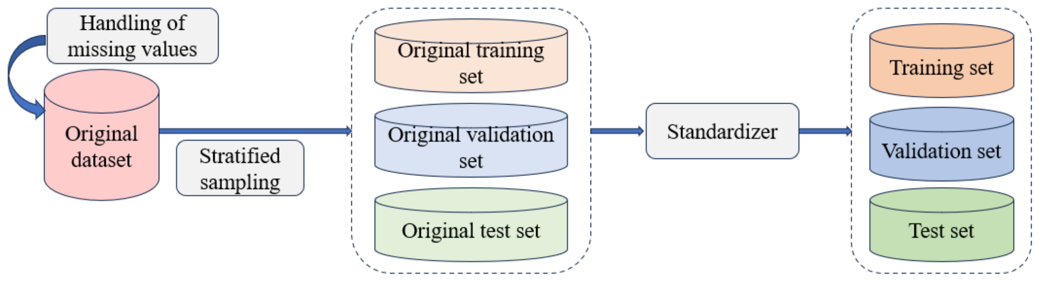
According to the above partitioning principles, the final sample distribution is as follows: the training set includes 771 distressed enterprises and 771 healthy enterprises; the validation set includes 258 distressed enterprises and 257 healthy enterprises; the test set includes 257 distressed enterprises and 258 healthy enterprises. The complete data screening and segmentation process is shown in Figure 6.

3.3.4. Standardization Processing

The Z-score normalization method is employed in this study to preprocess the input variables. Let the feature matrix of the training set be denoted as $\mathit{X}\in {ℝ}^{n\times 47}$, where $n$ represents the total number of training samples (including data from 771 financially distressed firms and 771 non-distressed firms over eight time steps, yielding a total of 12,336 sample data), and 47 denotes the number of financial feature indicators. The mathematical representation is given as follows:

$$\mathit{X}=\left[\begin{array}{cccc}{x}_{1,1}& x_{1,2}& \dots & x_{1,47}\\ x_{2,1}& x_{2,2}& \dots & x_{2,47}\\ ⋮& ⋮& \ddots & ⋮\\ x_{n,1}& x_{n,2}& \dots & x_{n,47}\end{array}\right]$$

(41)

For each financial feature column vector in $\mathit{X}$ denoted as ${\mathit{x}}^{(j)}={(x_{1,j},x_{2,j},\cdots ,x_{n,j})}^T,j=1,2,\cdots ,47$, standardization is performed as follows:

$${\widehat{x}}_{i,j}={\displaystyle \frac{x_{i,j}-{\overline{x}}_j}{s_j}}$$

(42)

In Equation (42), ${\widehat{x}}_{i,j}$ denotes the standardized value of the $i$-th sample on the $j$-th financial feature. Specifically, $x_{i,j}$ is the original value, ${\overline{x}}_j$ is the mean of feature $j$ in the training set, and $s_j$ is the corresponding standard deviation.

At the same time, to prevent data leakage from overestimating the model, this study only fits the standardized parameters on the training set: that is, we calculate the mean and standard deviation of each indicator in the original training set and save them in the standardizer, and then use the same set of parameters to perform consistent standardization transformation on the original validation set and the original test set.

After the above missing data processing, sample data division, and standardization processing, the final dataset that can be used for model training and evaluation is obtained, including the training set, validation set, and test set.

The data presented in this study is time-series data. For a single sample, the data input into the model includes 47 characteristic indicators over eight consecutive quarters. The specific matrix is as follows:

$$\mathit{M}=\left[\begin{array}{cccc}{\widehat{x}}_{t-8,1}& {\widehat{x}}_{t-8,2}& \dots & {\widehat{x}}_{t-8,47}\\ {\widehat{x}}_{t-7,1}& {\widehat{x}}_{t-7,2}& \dots & {\widehat{x}}_{t-7,47}\\ ⋮& ⋮& \ddots & ⋮\\ {\widehat{x}}_{t-1,1}& {\widehat{x}}_{t-1,2}& \dots & {\widehat{x}}_{t-1,47}\end{array}\right]$$

(43)

In Equation (43), ${\widehat{x}}_{r,j},r=t-8,t-7,\cdots ,t-1,j=1,2,\cdots ,47$ denotes the standardized value of the $j$-th feature indicator of an individual enterprise in period $r$. The input data of all enterprises are stacked into a three-dimensional tensor $\mathit{N}\in {ℝ}^{n\times 8\times 47}$, where $n$ is the number of enterprises, eight is the number of time steps, and 47 is the number of feature indicators. The model input sample set consists of the input tensor $\mathit{N}$ and the category label vector ${\mathit{y}}^{(t)}$, i.e., $\mathit{D}=(\mathit{N},{\mathit{y}}^{(t)})$, where each element in ${\mathit{y}}^{(t)}={(y_1^t,y_2^t,\cdots ,y_n^t)}^T,y_i^t=\{0,1\}$ is the category label of an enterprise, corresponding to the model’s output prediction for the last time step of that enterprise.

In addition, this study also incorporates baseline models such as LR, SVM, RF, and XGBoost for comparison. Because LR, SVM, RF, and XGBoost are not inherently designed for sequential data, this study transforms the historical observation data over eight quarters into static feature representations. Specifically, the original feature vector with 47 dimensions for each quarter is concatenated across an eight-quarter window, yielding a 376-dimensional composite feature vector as the input for each enterprise.

$$\mathit{O}=\left[\begin{array}{ccccc}{\widehat{\mathit{x}}}_1^{(t-8)}& {\widehat{\mathit{x}}}_1^{(t-7)}& \dots & {\widehat{\mathit{x}}}_1^{(t-2)}& {\widehat{\mathit{x}}}_1^{(t-1)}\\ {\widehat{\mathit{x}}}_2^{(t-8)}& {\widehat{\mathit{x}}}_2^{(t-7)}& \dots & {\widehat{\mathit{x}}}_2^{(t-2)}& {\widehat{\mathit{x}}}_2^{(t-1)}\\ ⋮& ⋮& & ⋮& ⋮\\ {\widehat{\mathit{x}}}_n^{(t-8)}& {\widehat{\mathit{x}}}_n^{(t-7)}& \dots & {\widehat{\mathit{x}}}_n^{(t-2)}& {\widehat{\mathit{x}}}_n^{(t-1)}\end{array}\right]$$

(44)

In Equation (44), ${\widehat{\mathit{x}}}_r^{(t)}\in {ℝ}^{1\times 47}$ denotes the standardized vector with 47 dimensions for the enterprise $r$ in quarter $t$, where $r=1,2,\cdots ,n$, and $t=t-8,t-7,\cdots ,t-1$. Here, $n$ is the number of enterprises.

4. Establishment of an Enterprise Financial Distress Early-Warning Model

4.1. The Construction Process of the Enterprise Financial Distress Early-Warning Model

This study is based on a deep learning time-series framework. A residual connection mechanism is introduced into the recurrent neural network to construct the RGRU model, which is used to effectively identify enterprise financial crises. At the same time, ablation experiments are designed from two dimensions: the type of recurrent units (GRU and LSTM) and the connection mechanism (residual connection and dense connection). Comparative models such as RLSTM, DGRU, and DLSTM are constructed under different network depths.

To ensure comparability among the different models, in the RGRU model and the comparison models RLSTM, DGRU, and DLSTM constructed in this study, consistency is maintained in the input and output feature dimensions at each layer and the network structure follows the principle of layer-by-layer feature modeling. The specific settings of the input and output dimensions for the RGRU and RLSTM models are given in

Table 4. Input and output feature dimensions for the five-layer residual fusion early-warning models.

Neural Network Layer	Input Size	Output Size	Explanation
GRU1 and LSTM1	47	32	Input size is 47 dimensions; output size is 32 dimensions.
GRU2 and LSTM2	32	64	Input size is 32 dimensions; output size is 64 dimensions.
Residual connection	47, 64	64	Input size is 47, 64 dimensions; output size is 64 dimensions.
GRU3 and LSTM3	64	128	Input size is 64 dimensions; output size is 128 dimensions.
GRU4 and LSTM4	128	256	Input size is 128 dimensions; output size is 256 dimensions.
Residual connection	47, 64, 256	256	Input size is 47, 64, 256 dimensions; output size is 256 dimensions
GRU5 and LSTM5	256	512	Input size is 256 dimensions; output size is 512 dimensions.

.

The input dimension of the first layer of the network is set to 47, which precisely corresponds to the comprehensive financial and governance indicator system constructed in this study. Regarding the setting of the output feature dimension, this study follows the dimension setting idea in the research by He et al. (2015) and Ren (2026), and sets the output feature dimensions of each layer as 32, 64, 128, 256, and 512 in sequence [13,25]. Specifically, in the constructed RGRU and RLSTM models, the 47-dimensional feature vector of the initial input is mapped by the first layer network to a 32-dimensional feature, and then the second layer network takes the 32-dimensional feature as input and outputs a 64-dimensional feature. In the first residual connection, the 47-dimensional feature vector of the initial input is aligned with the 64-dimensional output of the second layer through dimension mapping and fused using addition to form the 64-dimensional feature input of the third layer, which is then output as a 128-dimensional feature by the network. Subsequently, the 128-dimensional feature is input to the fourth layer network to obtain a 256-dimensional output. In the second residual connection, the 47-dimensional input, the 64-dimensional output of the second layer, and the 256-dimensional output of the fourth layer are aligned through dimension mapping and fused using addition to form the 256-dimensional input of the fifth layer, and finally output a 512-dimensional feature representation. In addition, in the empirical stage, this study also constructed a three-layer residual fusion architecture for comparison. This architecture only retains the first residual connection and enters the fully connected layer for prediction after outputting a 128-dimensional feature from the third layer.

In the ablation comparison experiment of the connection mechanism, this study conducts a comparative analysis using the dense connection architecture, and builds the DGRU and DLSTM models. The specific input and output feature dimensions are shown in

Table 5. The setting of input and output feature dimensions for the five-layer dense fusion early-warning model.

Neural Network Layer	Input Size	Output Size	Explanation
GRU1 and LSTM1	47	32	Input size is 47 dimensions; output size is 32 dimensions.
Dense connection	47, 32	79	Input size is 47, 32 dimensions; output size is 79 dimensions.
GRU2 and LSTM2	79	64	Input size is 79 dimensions; output size is 64 dimensions.
Dense connection	47, 32, 64	143	Input size is 47, 32, 64 dimensions; output size is 143 dimensions.
GRU3 and LSTM3	143	128	Input size is 143 dimensions; output size is 128 dimensions.
Dense connection	47, 32, 64, 128	271	Input size is 47, 32, 64, 128 dimensions; output size is 271 dimensions.
GRU4 and LSTM4	271	256	Input size is 271 dimensions; output size is 256 dimensions.
Dense connection	47, 32, 64, 128, 256	527	Input size is 47, 32, 64, 128, 256 dimensions; output size is 527 dimensions.
GRU5 and LSTM5	527	512	Input size is 527 dimensions; output size is 512 dimensions.

.

In addition, this study also constructs a three-layer dense fusion architecture for comparison. This architecture only retains the first two dense connections, and after the third-layer network outputs 128-dimensional features, it enters the fully connected layer to complete the prediction.

4.2. Hyperparameter Settings

Hyperparameters significantly affect the model’s performance, including its fitting ability, generalization, and training stability. This study considers three key hyperparameters: batch size, dropout rate, and training epochs. To avoid suboptimal manual tuning, grid search is adopted to exhaustively explore all parameter combinations within a predefined space. Each configuration is independently trained and evaluated, and the optimal set is selected based on the minimum validation loss. The optimization objective formula is as follows:

$$L=-{\displaystyle \frac{1}{N}}{\displaystyle \sum _{i=1}^N[y_i\log ({\widehat{y}}_i)+(1-}{y}_i)\log (1-{\widehat{y}}_i)]$$

(45)

In Equation (45), $N$ is the batch size, $y_i\in \{0,1\}$ is the true label of the $i$-th sample, and ${\widehat{y}}_i$ is the probability of financial distress for the $i$-th sample predicted by the model.

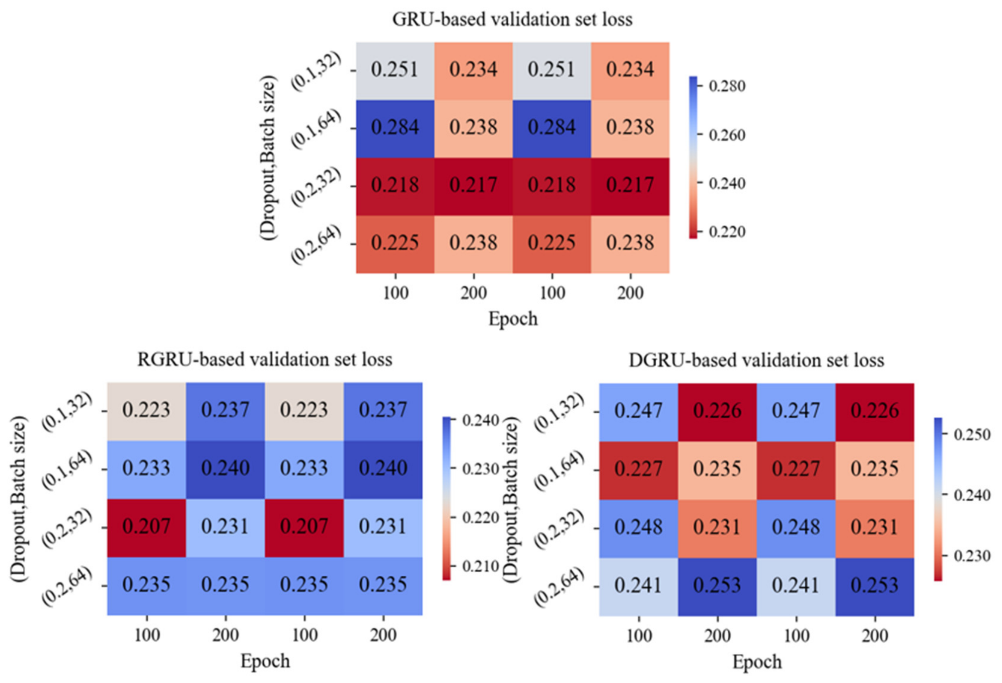
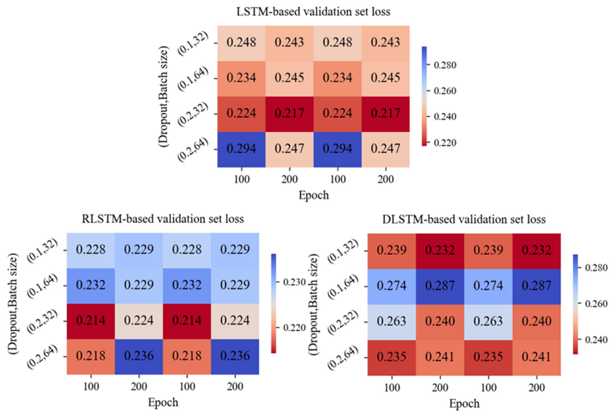
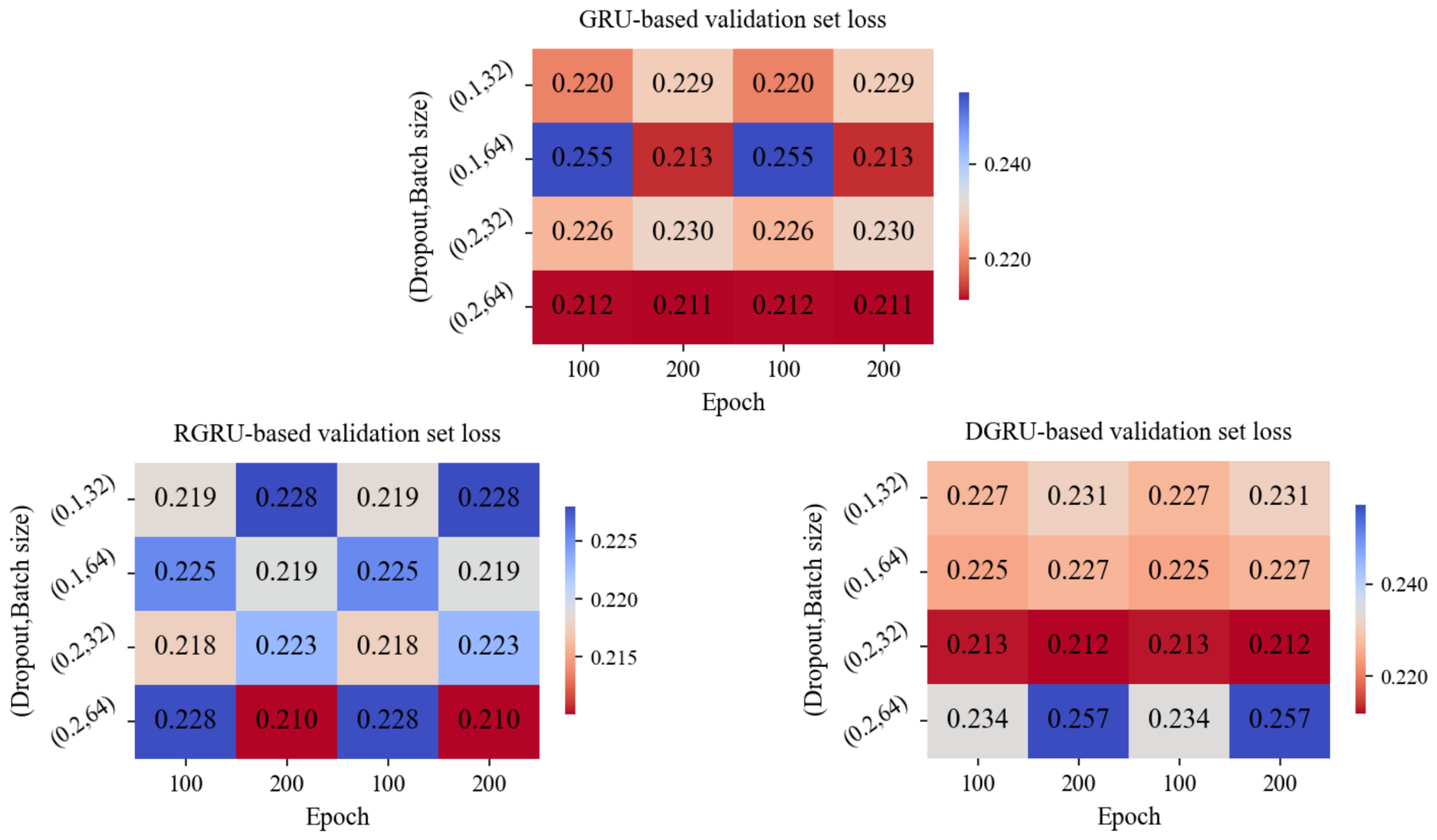
In the RGRU model and its ablation comparison models, because each model contains multiple sets of hyperparameters, in order to obtain a better hyperparameter combination, the grid search method is adopted to optimize the hyperparameters of the models. Figure 7 and Figure 8 show the heatmaps of the loss values of each model, respectively, on the validation set under different hyperparameter combinations. The color intensity in the figures reflects the performance of the models corresponding to different parameter combinations. The darker the red, the lower the loss on the validation set under that hyperparameter combination, and the better the generalization performance of the model.

The relevant configuration of the model and the implementation script are all included in the Supplementary Materials (Supplementary Folders S2 and S3).

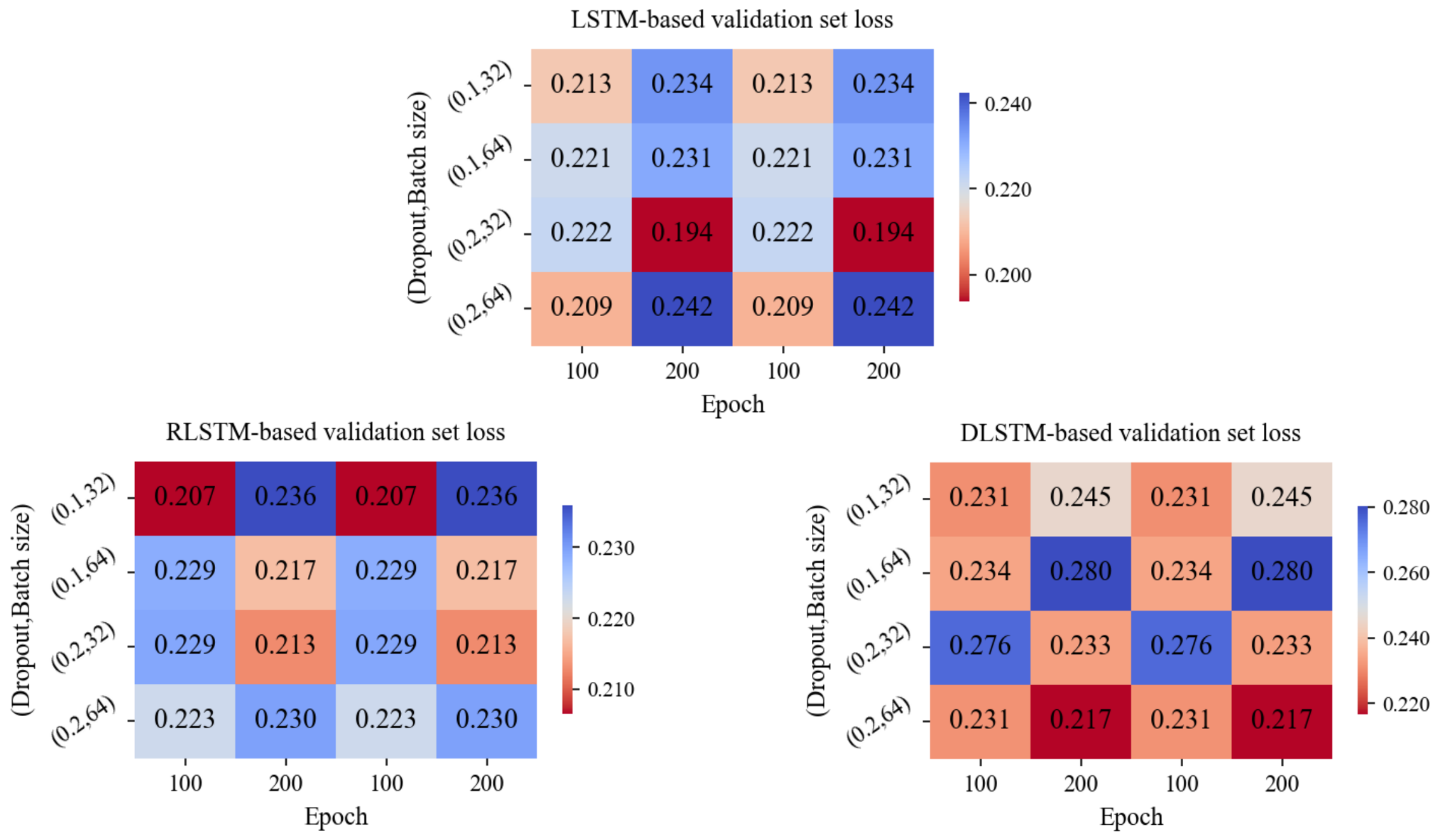
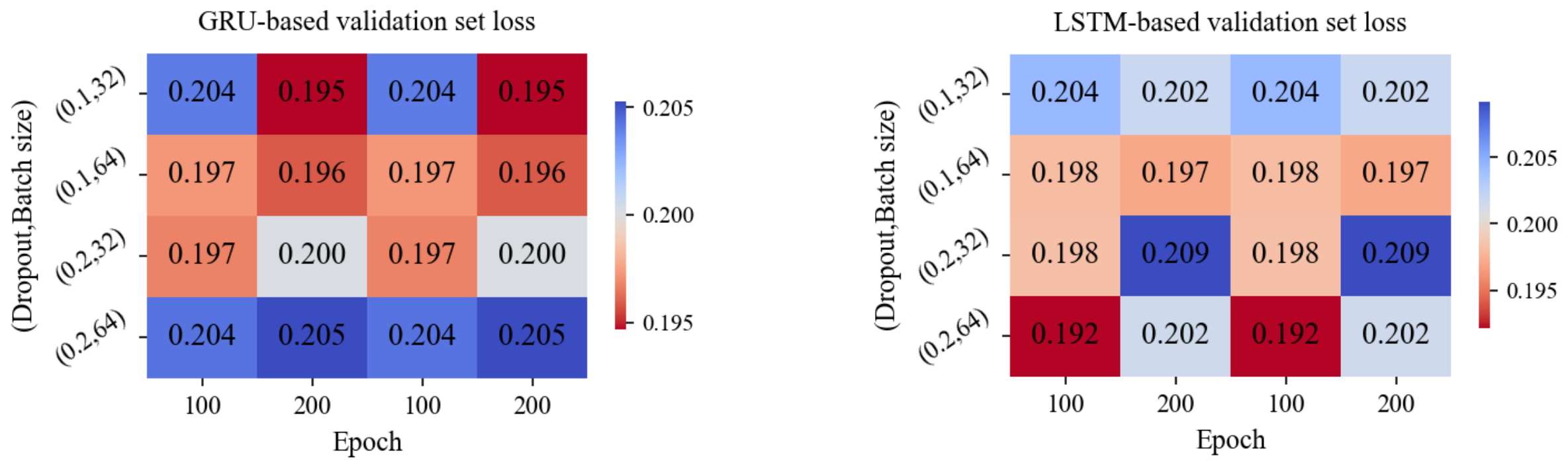
During the empirical stage, this study also constructed comparison models such as the RGRU model with a three-layer network depth, RLSTM, DGRU, and DLSTM, as well as the basic GRU model and LSTM model with a one-layer network depth, to be compared with the RGRU model with a five-layer network depth constructed in this study. The heatmaps of the loss values of each model on the validation set under different hyperparameter combinations are shown in Figure 9, Figure 10 and Figure 11.

The optimal hyperparameter combinations for each model were finally determined, and the results are given in

Table 6. Table of optimal hyperparameter combinations for each model.

Network Depth	Model	Dropout Rate	Batch Size	Epoch	Validation Loss
Five layers	GRU	0.2	32	200	0.217
	RGRU	0.2	32	100	0.207
	DGRU	0.2	32	200	0.226
	LSTM	0.2	32	200	0.217
	RLSTM	0.2	32	100	0.214
	DLSTM	0.1	32	200	0.232
Three layers	GRU	0.2	64	200	0.211
	RGRU	0.2	64	200	0.210
	DGRU	0.2	32	200	0.212
	LSTM	0.2	32	200	0.194
	RLSTM	0.1	32	100	0.207
	DLSTM	0.2	64	200	0.217
One layer	GRU	0.1	32	200	0.195
	LSTM	0.2	64	100	0.192

Note: Bold values indicate the lowest validation loss achieved by the five-layer RGRU model constructed in this study.

.

As shown in Table 6, the five-layer RGRU model constructed in this study achieved the lowest loss value of 0.207 in the validation stage, indicating that this model has a better fitting effect and generalizability under the current parameter configuration. Based on this optimal hyperparameter combination, the model’s predictive performance was further evaluated on the test set.

4.3. Other Experimental Details

The hyperparameter settings in this experiment were selected based on commonly adopted empirical ranges in the literature and preliminary validation experiments. The details of other experiments for each of the above models, including all the parameters involved in the models, are shown in

Table 7. Table of optimal hyperparameter combinations for each model.

Model	Dropout Rate
GRU, RGRU, DGRU, LSTM, RLSTM, DLSTM	Optimizer: Adam; learning rate: 0.001; loss function: cross-entropy loss; random seed: 42
LR	Max iter: 500; random seed: 42; class weight: balanced
SVM	C = 2; kernel: rbf; gamma: 0.02; probability: True; random seed: 42
RF	N estimators: 400; max depth: 25; min samples_split: 5; min_samples_leaf: 2; max features: sqrt; bootstrap: True; oob score: True; random seed: 42
XGBoost	N_estimators: 100; max_depth: 4; learning_rate: 0.1; subsample: 0.8; colsample_bytree: 0.8; objective: binary:logistic; eval_metric: logloss; random seed: 42; use_label_encoder: False

.

4.4. Evaluation Metrics

In a binary classification task, the classification results have two types: positive and negative. In this study, the positive samples are distress enterprises with high financial risks, and the negative samples are normal enterprises. Based on the model’s prediction results and the actual categories of the samples, four basic situations can be obtained: True Positive (TP), False Positive (FP), True Negative (TN), and False Negative (FN). If the model’s prediction result is the same as the sample’s actual category, it is true; otherwise, it is false. The structure of the confusion matrix is shown in

Table 8. Confusion matrix.

Classification Results		Prediction Classification
		Positive Sample	Negative Sample
Actual classification	Positive sample	TP	FN
	Negative sample	FP	TN

.

This study has constructed a classification evaluation system based on the confusion matrix. Specifically, it includes five evaluation indicators: accuracy, precision, recall, F1 score, and AUC value. Among them, accuracy measures the proportion of correctly classified samples across the entire dataset, with values closer to 1 indicating better overall classification performance. Precision represents the proportion of samples predicted as ST that are indeed ST. Recall reflects the proportion of actual ST samples correctly identified by the model. The F1 score, defined as the harmonic mean of precision and recall, approaches 1 when the model achieves a favorable balance between the two. The AUC refers to the area under the Receiver Operating Characteristic (ROC) curve, where the false positive rate (FPR) is plotted on the x-axis and the true positive rate (TPR, equivalent to recall) on the y-axis. A higher AUC value, approaching 1, indicates stronger discriminative capability of the model. The mathematical definitions of these metrics are provided as follows:

$$\mathrm{Accuracy}={\displaystyle \frac{\mathrm{T}\mathrm{P}+\mathrm{T}\mathrm{N}}{\mathrm{T}\mathrm{P}+\mathrm{F}\mathrm{P}+\mathrm{T}\mathrm{N}+\mathrm{F}\mathrm{N}}}\times 100\%$$

(46)

$$\mathrm{P}\mathrm{r}\mathrm{e}\mathrm{c}\mathrm{i}\mathrm{s}\mathrm{i}\mathrm{o}\mathrm{n}={\displaystyle \frac{\mathrm{T}\mathrm{P}}{\mathrm{T}\mathrm{P}+\mathrm{F}\mathrm{P}}}\times 100\%$$

(47)

$$\mathrm{R}\mathrm{e}\mathrm{c}\mathrm{a}\mathrm{l}\mathrm{l}=\mathrm{T}\mathrm{P}\mathrm{R}={\displaystyle \frac{\mathrm{T}\mathrm{P}}{\mathrm{T}\mathrm{P}+\mathrm{F}\mathrm{N}}}\times 100\%$$

(48)

$$\mathrm{F}1 \mathrm{s}\mathrm{c}\mathrm{o}\mathrm{r}\mathrm{e}=2\times {\displaystyle \frac{\mathrm{A}\mathrm{c}\mathrm{c}\mathrm{u}\mathrm{r}\mathrm{a}\mathrm{c}\mathrm{y}\times \mathrm{R}\mathrm{e}\mathrm{c}\mathrm{a}\mathrm{l}\mathrm{l}}{\mathrm{A}\mathrm{c}\mathrm{c}\mathrm{u}\mathrm{r}\mathrm{a}\mathrm{c}\mathrm{y}+\mathrm{R}\mathrm{e}\mathrm{c}\mathrm{a}\mathrm{l}\mathrm{l}}}\times 100\%$$

(49)

$$\mathrm{F}\mathrm{P}\mathrm{R}={\displaystyle \frac{\mathrm{F}\mathrm{P}}{\mathrm{F}\mathrm{P}+\mathrm{T}\mathrm{N}}}\times 100\%$$

(50)

5. Model Training and Results Analysis

5.1. Performance Evaluation and Analysis of Basic Models with Different Network Depths

To verify the rationality and effectiveness of the architectural optimization introduced by the deep network structure, this section conducts an empirical analysis on a test set consisting of 257 enterprises in financial distress and 258 normal enterprises. Under different network depths (one layer, three layers, and five layers), the prediction performance of the basic GRU and LSTM models is comprehensively evaluated based on five evaluation indicators: accuracy, precision, F1 score, recall, and AUC value. The results are provided in

Table 9. Comparison of model performance with different network depths.

Network Depth	Model	Accuracy (%)	Precision (%)	F1 Score (%)	Recall (%)	AUC
Five layers	GRU	88.16	90.16	87.82	85.60	0.9290
	LSTM	88.93	88.46	88.97	89.49	0.9564
Three layers	GRU	90.49	92.28	90.26	88.33	0.9584
	LSTM	88.74	88.12	88.80	89.49	0.9537
One layer	GRU	88.93	90.00	88.76	87.55	0.9387
	LSTM	89.13	89.41	89.06	88.72	0.9431

.

As shown in Table 9, network depth exerts a significant influence on the prediction performance of both GRU and LSTM models. Overall, with an increase in network depth, the two baseline models do not show a trend of continuous improvement across all evaluation metrics.

Specifically, the GRU model achieves the best performance at the three-layer depth, with an accuracy of 90.49% and an AUC value of 0.9584. However, its performance drops significantly when the network depth increases to five layers, with the accuracy decreasing to 88.16% and the AUC value dropping to 0.9290. For the LSTM model, although its AUC value gradually increases from 0.9431 at the one-layer depth to 0.9537 at three layers and 0.9564 at five layers, its accuracy is 89.13% at the one-layer structure, and decreases to 88.74% and 88.93% at the three-layer and five-layer structures, respectively. In addition, on the three metrics of precision, F1 score, and recall, neither model demonstrates the characteristic of steady performance improvement as the network deepens.

These results indicate that merely increasing the depth of the network may cause the model to be affected by difficulties in gradient propagation, information attenuation, and parameter redundancy during the training process. This, in turn, weakens the effective transmission and utilization of temporal information, restricting the further improvement of the model’s performance. Therefore, it is necessary to conduct targeted architectural optimization of the deep network structure to alleviate the problem of gradient disappearance in deep networks and enhance the model’s expressive ability in complex tasks.

5.2. Performance Evaluation and Analysis of Improved Models Under Different Network Depths

Based on the comparative analysis of baseline GRU and LSTM at different depths in Section 5.1, this study introduces residual connections to construct the RGRU model and sets up ablation experiments including dense connections and LSTM structures. Each model is systematically evaluated under different network depths to verify the effectiveness and stability of the five-layer RGRU model.

5.2.1. Analysis of Model Performance at a Three-Layer Network Depth

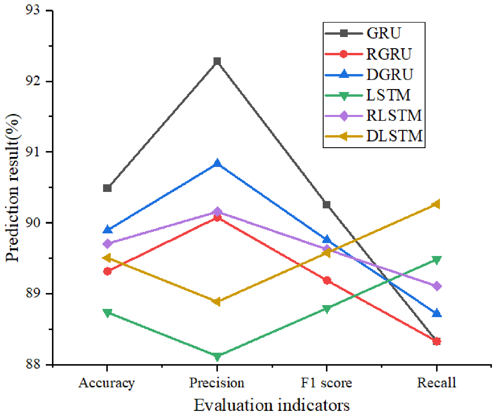
Based on the optimal hyperparameter combination determined in Section 4.2 for the three-layer network, predictions are made on the test set, and the results are given in

Table 10. Comparison results of prediction performance of each model under three-layer network depth.

Model	Accuracy (%)	Precision (%)	F1 Score (%)	Recall (%)	AUC
GRU	90.49	92.28	90.26	88.33	0.9584
RGRU	89.32	90.08	89.19	88.33	0.9579
DGRU	89.90	90.84	89.76	88.72	0.9605
LSTM	88.74	88.12	88.80	89.49	0.9537
RLSTM	89.71	90.16	89.63	89.11	0.9480
DLSTM	89.51	88.89	89.63	90.27	0.9621

. At the same time, the performance of RGRU and the comparison models is visualized through a line graph (Figure 12) to analyze the impact of the structural improvement at this depth.

(1)

Analysis of prediction results of RGRU and RLSTM models

As can be observed from Table 8 and Figure 12, under the three-layer network depth, the RGRU model does not achieve better performance than the baseline GRU model. It achieves an accuracy of 89.32%, a precision of 90.08%, and an F1 score of 89.19%, which are decreased by 1.17%, 2.20%, and 1.07%, respectively, compared with the baseline GRU model, indicating an overall decline in classification performance. Meanwhile, its AUC value is 0.9579, which is basically equivalent to the 0.9584 of the baseline GRU model. This reveals that the introduction of residual connections fails to significantly improve model performance at this network depth. A possible reason lies in the limited benefit of cross-layer information fusion in shallow networks and the increased structural complexity, which weakens the original efficient feature representation capability of the GRU model.

In comparison, the RLSTM model achieves certain improvements in several metrics. Its accuracy, precision, and F1 score reach 89.71%, 90.16%, and 89.63%, respectively, all of which are improved to some extent relative to the baseline LSTM model. However, its recall and AUC value are 89.11% and 0.9480, slightly lower than those of the baseline model. This indicates that, while the model enhances partial classification performance, there still exists certain fluctuation in the stability of its overall classification discrimination.

(2)

Analysis of prediction results of DGRU and DLSTM model

To further evaluate the optimization effect of different connection mechanisms on the GRU model, this study constructs the DGRU model with a dense connection mechanism. As shown in Table 8 and Figure 12, compared with the basic GRU model, the DGRU model has an improved recall and AUC value, which are 88.72% and 0.9605, respectively. However, its accuracy, precision, and F1 score are 89.90%, 90.84%, and 89.76%, respectively, which are slightly lower than those of the basic GRU model. These results indicate that the dense connection enhances the feature reuse ability and brings certain improvements in some evaluation indicators, but fails to achieve consistent improvement in all indicators, and the overall performance improvement is still relatively limited.

The DLSTM model’s accuracy, precision, F1 score, and recall are improved by 0.77%, 0.77%, 0.83%, and 0.78%, respectively, when compared with the basic LSTM model, and the AUC value reaches 0.9621. This result shows that the dense connection mechanism enhances the feature extraction ability and discriminative performance of the LSTM model to a certain extent, but the overall performance improvement is relatively limited.

Overall, at the three-layer network depth, residual connection and dense connection both have certain effects on the performance of different recurrent neural network models, but they show local indicator optimization rather than consistent overall performance improvement. This indicates that, at the current network depth setting, the basic GRU and LSTM models have already demonstrated relatively strong temporal information modeling capabilities in this task. At this point, the performance gain brought by further introducing architecture optimization is relatively limited. At the same time, the performance of the two connection mechanisms in GRU and LSTM models is different, indicating that the effectiveness of architecture improvement is not only related to the connection method, but may also be affected by the characteristics of the basic recurrent unit structure.

5.2.2. Analysis of Model Performance at Five-Layer Network Depth

Further analysis was conducted on the impact of network depth on model performance. Based on the five-layer RGRU model constructed in Section 2.3 and the ablation comparison model (RLSTM, DLSTM, and DGRU) constructed in Section 2.4, combined with the optimal hyperparameter combination determined in Section 4.2, prediction experiments were carried out on the test set. The results are provided in

Table 11. Comparison results for prediction performance of each model under five-layer network depth.

Model	Accuracy (%)	Precision (%)	F1 Score (%)	Recall (%)	AUC
GRU	88.16	90.16	87.82	85.60	0.9290
RGRU	91.65	90.53	91.75	93.00	0.9606
DGRU	88.54	91.25	88.13	85.21	0.9555
LSTM	88.93	88.46	88.97	89.49	0.9564
RLSTM	91.26	90.46	91.33	92.22	0.9591
DLSTM	90.10	88.72	90.25	91.83	0.9632

Note: The bolded row represents the core model constructed in this study.

. Additionally, the prediction results of each model were visualized through line graphs (see Figure 13) to analyze the impact of architecture improvements on model performance under a five-layer network depth.

(1)

Analysis of prediction results of RGRU and RLSTM models

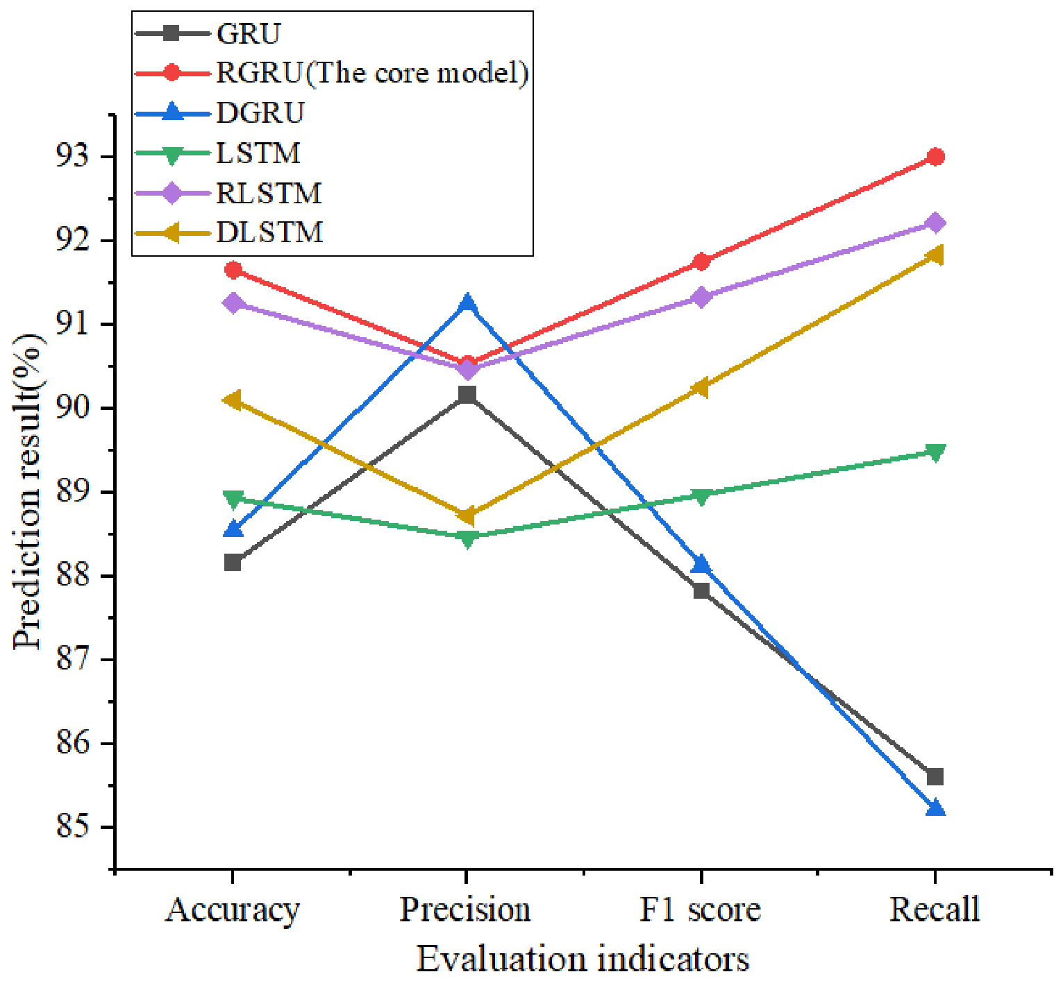
As can be seen from Table 9 and Figure 13, the RGRU model outperforms the basic GRU model in overall performance when the network depth reaches five layers. Its accuracy is 91.65%, the F1 score is 91.75%, and the recall is 93.00%, which are 3.49%, 3.93%, and 7.4% higher than those of the basic GRU model, respectively. This indicates that the residual connection mechanism helps improve the model’s ability to identify positive samples in deep networks. At the same time, the AUC value of the RGRU model reaches 0.9606, which is significantly higher than that of the basic GRU model (0.9290), indicating that the overall discriminative and ranking abilities of the model have also been improved. Specifically, the RGRU model maintains a high recall while also achieving a high precision, demonstrating better balance, which gives it strong application potential in enterprise financial distress warning tasks and enables it to control the error rate while reducing the risk of missed judgments.

When comparing with the model RLSTM, its accuracy is 91.26%, the precision is 90.46%, the F1 score is 91.33%, the recall is 92.22%, and the AUC value is 0.9591. The various indicators of the model have been improved to varying degrees compared to the basic LSTM model. This indicates that, when the network reaches a sufficient depth, the problem of vanishing gradients in deep networks becomes prominent, and the residual connection can effectively alleviate this problem and exert its architectural advantages, verifying that the residual connection also has good applicability and effectiveness in deep LSTM networks. However, compared with the RGRU model, the prediction results of the RLSTM model are all worse, indicating that the fusion effect of residual connection with GRU is better than that with LSTM in this experiment.

(2)

Analysis of prediction results of DGRU and DLSTM model

In the contrast model with the dense connection mechanism, the DGRU model achieved an accuracy of 91.25%, which was the best among the five-layer network models. Meanwhile, its accuracy was 88.54% and the F1 score was 88.13%, which were 0.38% and 0.31% higher than those of the basic GRU model, respectively. The AUC value also increased to 0.9555, indicating that the dense connection, through feature reuse, can enhance the discriminative ability of the model to a certain extent. However, its recall dropped to 85.21%, suggesting that although the introduction of the dense connection played a certain role, it also led to a certain degree of weakening of the model’s ability to identify positive samples, resulting in a certain imbalance in the overall performance of the model.

Compared with other models, the DLSTM model performed the best in terms of the AUC value, reaching 0.9632, demonstrating the positive effect of the dense connection mechanism in improving the discriminative stability of the LSTM model. Its accuracy, precision, F1 score, and recall reached 90.10%, 88.72%, 90.25%, and 91.83%, respectively; although they were lower than those of the RGRU model, they were all better than those of the basic LSTM model. This further verifies the effectiveness of the dense connection mechanism in improving the efficiency of model information flow, but its comprehensive classification ability is still slightly weaker than that of the RGRU model.

Overall, at the five-layer network depth, both residual connection and dense connection can improve the model’s performance to a certain extent. However, compared with the dense connection, the improvement effect of the residual connection is more comprehensive and stable. In particular, the RGRU model, which is integrated by residual connections, demonstrates superior performance in comprehensive classification capabilities. Especially in terms of accuracy, F1 score, and recall, it outperforms the RLSTM, DGRU, and DLSTM comparison models. Therefore, in the deep network structure, introducing residual connections to improve the architecture of GRU is effective and can enhance the training performance in the deep network, while also improving the overall prediction performance and stability of the model.

5.3. ROC Curves of Each Model at a Five-Layer Network Depth

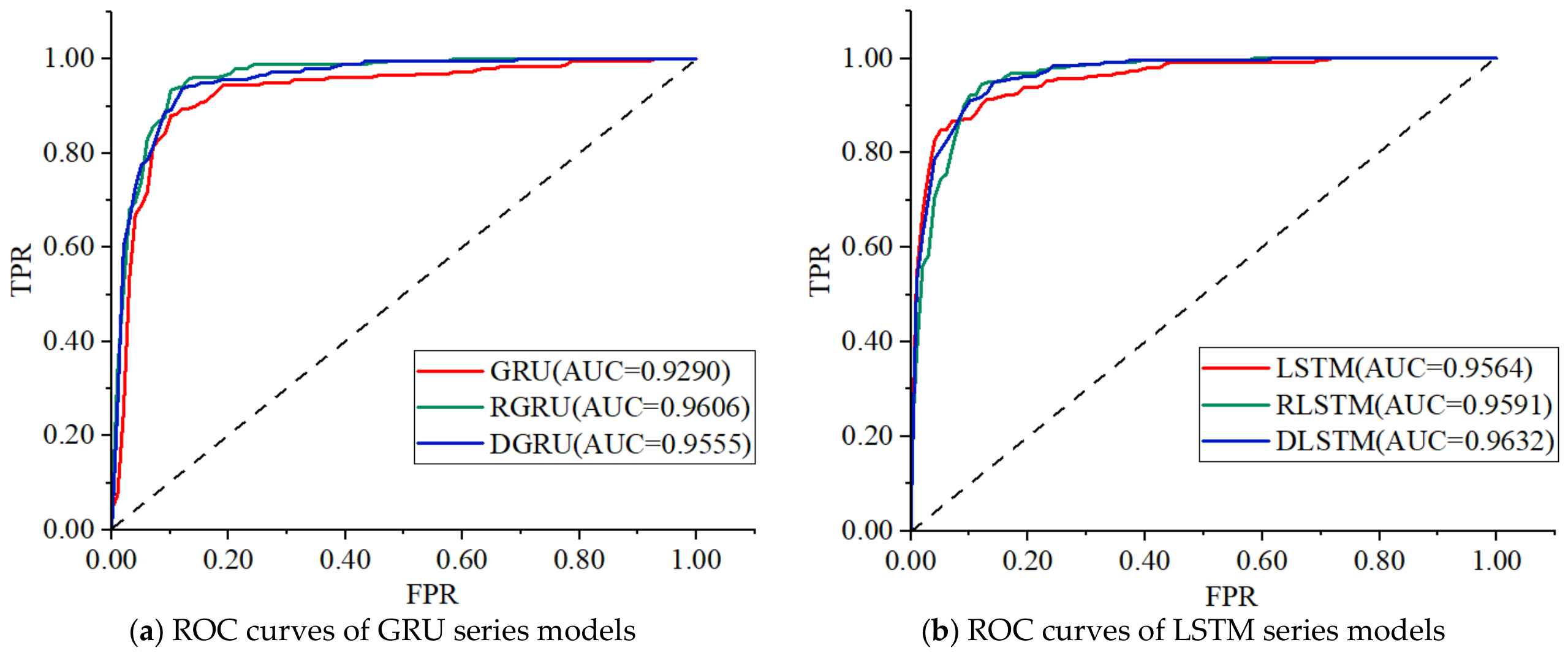
The ROC curve can comprehensively depict the classification performance of the model under different risk tolerance levels. To further analyze the effectiveness of the RGRU model constructed in this study, in this section, the ROC curves of the GRU series and the LSTM series are plotted separately, as shown in Figure 14.

It can be seen from Figure 14a that the ROC curve of the RGRU model is closer to the upper left corner, significantly deviating from the random baseline. Its AUC value (0.9606) is significantly higher than that of the GRU model (0.9290). This indicates that the RGRU model has excellent binary classification discrimination ability. Especially in the low-false-positive-rate range, the RGRU model achieved a higher true rate, indicating that it can effectively identify more enterprises in financial distress under strict control of the false alarm rate. This result further verifies the significant advantage of residual connection in improving the early risk identification ability of the model.

Figure 14b shows that the AUC value of the DLSTM model is the highest in the LSTM series, and it exhibits stronger overall sorting ability in the medium-high-false-positive-rate range, reflecting the positive role of dense connection in promoting the fusion of model complex features and enhancing deep feature expression. It is worth noting that, although the AUC value of the DLSTM model is slightly higher than that of the RGRU model, when combined with the results in Table 11 the high AUC value of the DLSTM model did not translate into its advantages in accuracy (90.10%) and F1 score (90.25%). This indicates that, in the enterprise financial distress warning task, there is a certain deviation between the overall sorting ability reflected by the AUC value and the final classification performance. In contrast, the RGRU model achieved a better balance between classification accuracy and stability, while the DLSTM model is more focused on improving sorting ability, and its comprehensive applicability in actual classification decision tasks is relatively limited.

5.4. Quantitative Analysis of the Prediction Results of Each Model Under a Five-Layer Network Depth

In this section, the Brill score and logarithmic loss are further employed to quantitatively evaluate the probability prediction quality of the RGRU model at the five-layer network depth and the ablation comparison model. Among them, the Brillouin score measures the overall calibration level of probability predictions by calculating the mean square difference between the predicted probability and the actual result. This metric depicts the degree of deviation between the predicted probability and the actual observed result, thereby effectively reflecting the reliability of the model’s risk assessment. When the Brillouin score is low, it indicates that the risk probability output by the model is closer to the actual occurrence probability. The specific formula is as follows:

$$\mathrm{B}\mathrm{r}\mathrm{i}\mathrm{e}\mathrm{r} \mathrm{s}\mathrm{c}\mathrm{o}\mathrm{r}\mathrm{e}={\displaystyle \frac{1}{N}}{\displaystyle \sum _{i=1}^N{({\widehat{y}}_i-y_i)}^2}$$

(51)

In Equation (51), $N$ denotes the total number of samples, $y_i\in \{0,1\}$ represents the true class label of the $i$-th sample, and ${\widehat{y}}_i$ is the model-predicted probability of financial distress occurrence for the $i$-th sample.

The logarithmic loss is calculated based on the cross-entropy loss function and is used to measure the deviation between the predicted probability distribution of the model and the true labels. This metric imposes a higher penalty on samples with high confidence but incorrect predictions, thereby effectively suppressing the model’s overly confident prediction behavior. The smaller the value, the more accurately the model depicts the risk level of the sample, and the higher the consistency between the probability output and the true result. The specific formula is as follows:

$$\mathrm{L}\mathrm{o}\mathrm{g} \mathrm{l}\mathrm{o}\mathrm{s}\mathrm{s}=-{\displaystyle \frac{1}{N}}{\displaystyle \sum _{i=1}^N[y_i\log ({\widehat{y}}_i)+(1-y_i)\log (1-{\widehat{y}}_i)]}$$

(52)

In Equation (52), $N$ denotes the total number of samples, $y_i\in \{0,1\}$ represents the true class label of the $i$-th sample, and ${\widehat{y}}_i$ is the model-predicted probability of financial distress occurrence for the $i$-th sample.

The results of each model in terms of the above two probability indicators are presented in

Table 12. Quantization comparison results of GRU-series models under five-layer network depth.

Model	Brier Score	Log Loss
GRU	0.1108	0.6691
RGRU	0.0772	0.4504
DGRU	0.1017	0.8589

and

Table 13. Quantization comparison results of LSTM-series models under five-layer network depth.

Model	Brier Score	Log Loss
LSTM	0.1020	0.6376
RLSTM	0.0828	0.5486
DLSTM	0.0888	0.6709

, respectively.

It can be seen that, in terms of probability prediction accuracy, the RGRU model and RLSTM model with the residual connection mechanism have significantly lower Brier scores and log loss compared to the basic GRU and LSTM models. This indicates that residual connection can effectively improve the probability prediction accuracy of the model.

In particular, the five-layer RGRU model proposed in this study performs the best, with the Brier score and log loss being the lowest among all models, at 0.0772 and 0.4504, respectively. This shows that residual connection not only alleviates the gradient problem of deep GRU, but also significantly enhances the calibration accuracy and reliability of the model’s predicted probability, making it more accurate in risk quantification for financial warning tasks.

In contrast, the RLSTM model is superior to the basic LSTM model in probability indicators, but its Brier score (0.0798) and log loss (0.4671) are still significantly higher than those of the RGRU model. The DGRU model and DLSTM model are superior to the corresponding basic models in Brier score, but their log loss is even higher than that of the corresponding basic models, with a limited reduction, and both indicators have not reached the level of the RGRU model. This reflects the deficiency of dense connection in improving the stability of probability prediction.

The above results collectively indicate that, in deep network structures, residual connection has a significant advantage over dense connection in improving the probability calibration ability of the model, and the combination of residual connection and GRU further transforms this advantage into comprehensive and stable probability prediction performance, thus demonstrating stronger applicability in this enterprise financial distress warning task.

5.5. Computational Efficiency of the Model Under a Five-Layer Network Depth

To further evaluate the computational efficiency and complexity of each model, this study compares the differences in computational resource consumption between the RGRU model and the ablation comparison model in terms of training time and parameter quantity on the test set. All the experiments were implemented in the PyTorch 3.12 deep learning framework under the Python 3.12 environment, and were completed on a system equipped with an Intel Core i5-9300H processor and a NVIDIA GeForce GTX 1650 graphics card. The relevant experimental results are shown in

Table 14. Training time and parameter size of five-layer models under optimal hyperparameter combinations.

Model	Optimal Hyperparameter Combination	Training Time (s)	Parameter Count (M)
GRU	[0.2, 32, 200]	76.25	1.58
RGRU	[0.2, 32, 100]	45.26	1.61
DGRU	[0.1, 32, 200]	86.50	2.15
LSTM	[0.2, 32, 200]	85.10	2.11
RLSTM	[0.2, 32, 100]	46.52	2.14
DLSTM	[0.1, 32, 200]	133.28	2.87

.

The RGRU model achieves a better balance between performance improvement and efficiency. Under the optimal parameter combination, the training time of the RGRU model is 45.26 s, and the parameter size is 1.61 megabytes. Compared with the basic GRU model, its training time is 30.99 s less, and the parameter size only increases by 0.03 megabytes. Among all the improved models with connection mechanisms introduced, it has the highest efficiency. The training time of the RLSTM model is 46.52 s, and the parameter size is 2.14 megabytes. Compared with the basic LSTM model, its training time is 38.58 s less, and the parameter size also only increases by 0.03 megabytes. In contrast, the introduction of dense connection mechanisms incurs certain additional computational and parameter costs. Specifically, the training time of the DGRU model and the DLSTM model is 86.50 s and 133.28 s, respectively, with parameter sizes of 2.15 megabytes and 2.87 megabytes, respectively. Compared with the base model, their training time is 10.25 s and 48.18 s longer, and their parameter sizes are 0.57 megabytes and 0.76 megabytes, respectively.

Overall, in deep temporal modeling, residual connection is a more efficient architectural improvement strategy. The RGRU model performs best in terms of training speed, parameter efficiency, and final performance. In this enterprise financial distress early-warning model, it achieves high prediction accuracy and operational efficiency. Although dense connection can improve performance to a certain degree, this improvement depends on the basic network structure, and it also generates higher computational and parameter costs.

5.6. Comparison of Other Models

Under the same test set, experiments were conducted on LR, SVM, RF, and XGBoost, and their performance results are given in

Table 15. Results of comparison of RGRU with other baseline models.

Model	Accuracy (%)	Precision (%)	F1 Score (%)	Recall (%)	AUC
LR	84.66	86.48	84.23	82.10	0.9171
SVM	81.94	78.87	82.81	87.16	0.9066
RF	93.98	91.24	94.16	97.28	0.9822
XGBoost	95.15	93.28	95.24	97.28	0.9886
RGRU	91.65	90.53	91.75	93.00	0.9606

Note: The bolded row represents the core model constructed in this study.

.

LR and SVM had the poorest overall discriminative performance, with accuracy rates of only 84.66% and 81.94%, respectively, and AUC values all below 0.92. Among them, the LR model had an accuracy rate of 86.48%, but a recall rate of only 82.10%, indicating a higher risk of missing financial crisis samples; the SVM model had a recall rate of 87.16%, slightly higher than LR, but an accuracy rate of only 78.87%, being the lowest among all models. It also misclassified a significant proportion of normal enterprises as risky enterprises, resulting in an overall F1 score of only 82.81%. The two linear models were limited by their linear fitting capabilities, were unable to explore the complex nonlinear correlations among multiple quarterly financial indicators, and were unable to adapt to high-dimensional financial early-warning tasks.

RF and XGBoost achieved the best static classification results based on the flattened static time-series features. Among them, XGBoost was the best for the entire model, with an accuracy rate of 95.15%, an accuracy rate of 93.28%, an F1 score of 95.24%, and an AUC of 0.9886. All the core indicators were globally leading. The RF model performed secondary, with an accuracy rate of 93.98%, and a recall rate that was the same as XGBoost, both reaching 97.28%. Both models had extremely strong identification capabilities for financial crisis samples and a very low risk of missed detection. Tree models do not need to model time-series dependencies and can only rely on static financial features to explore nonlinear discriminant rules. They have a natural advantage in cross-sectional financial data classification tasks at a single point in time.

The RGRU constructed in this study outperformed the LR and SVM linear models in all indicators, verifying the optimization effect of the time-series modeling mechanism and residual structure on deep recurrent networks. Although its static classification accuracy was slightly lower than the ensemble tree model, the recall rate of RGRU reached 93.00%, much higher than that of the linear models, and it retained the complete eight-quarter time-series information, capable of capturing the progressive deterioration pattern of enterprise financial risks year-by-year. In the rolling dynamic long-term risk warning scenarios, it possesses advantages in time-series modeling and interpretation that cannot be replaced by tree models.

6. Conclusions

This study focuses on the issue of enterprise financial distress warning. Within the framework of deep learning time-series modeling, it improves the traditional GRU model and introduces the residual connection mechanism to construct the RGRU model. It also conducts ablation experiments from two dimensions: the type of recurrent unit and the connection mode. At the same time, using the data of Chinese A-share listed companies from 2010 to 2024 as a sample, an empirical study is carried out. The main conclusions are as follows:

First, in terms of theory and methods, this study introduces the residual connection mechanism to the enterprise financial distress warning problem, constructs the RGRU model and, by introducing residual connections between multiple layers of GRU, builds a cross-layer identity mapping information transmission path, effectively alleviating the problem of gradient disappearance and performance degradation in deep networks, while improving the model’s ability to capture complex time-series features. At the same time, as ablation comparison models, the RLSTM, DGRU, and DLSTM models are designed for enterprise financial distress warning problems.

Second, in terms of model performance, the five-layer RGRU model constructed in this study outperforms the comparison models (e.g., RLSTM, DGRU, and DLSTM) in terms of accuracy, F1 score, and recall, and its AUC value reaches 0.9606. At the same time, it performs optimally in the Brillouin score and logarithmic loss probability prediction indicators, indicating its better prediction calibration ability. Moreover, through a comparison of the model training time and parameter quantity, it is verified that this model’s training efficiency is effectively improved.

Third, in terms of the comparison models, the empirical results show that, with a five-layer network depth, although dense connections can improve the model’s expression ability to a certain extent through feature concatenation operations, this performance improvement is somewhat unstable and accompanied by higher parameter complexity and computational overhead. In contrast, residual connections show stronger stability and applicability in deep networks.

In addition to the internal ablation experiments, we also introduced the complete spectrum of the mainstream tabular machine learning benchmark datasets for cross-paradigm validation. The proposed RGRU outperformed the linear statistical baseline methods (LR, SVM) on all core evaluation metrics, with the highest accuracy improvement reaching 9.71% (compared to SVM), and the recall rate increasing from 82.10% to 93.00%; at the same time, it retains the complete ordered time-series information, allowing it to track dynamic risk evolution and providing irreplaceable practical value for rolling long-term early warning in financial scenarios. Compared to tree-based ensemble models (such as XGBoost or RF), that can achieve higher prediction accuracy on the horizontally expanded static feature matrix, it also has certain modeling value. In summary, through architectural innovation and empirical verification, this study verifies the effectiveness and applicability of the RGRU model in the field of enterprise financial distress warning, not only improving the model’s prediction accuracy but also providing a new technical path for the application of deep time-series networks in financial risk management.

Despite the systematic exploration of model architecture optimization and empirical verification in enterprise financial distress early warning, this study still has limitations and room for further improvement. Future research can be extended in two main directions.

First, multi-source data including macroeconomic indicators, industry heterogeneity, and unstructured text data can be integrated to construct a more comprehensive early-warning system. This study uses an artificially matched one-to-one balanced sample for model structure comparison experiments, effectively avoiding the interference of class imbalance on algorithm performance comparisons. However, this sample construction method changes the natural proportion of distressed enterprises and healthy listed enterprises in the actual capital market. Therefore, the reported prediction indicators will have an optimistic bias relative to the actual deployment scenarios. When researchers apply the proposed RGRU model to the real financial-distress early-warning system, they need to retrain and calibrate the model using the naturally imbalanced samples in the original data and adopt imbalance optimization strategies such as weighted loss functions or adjustment of prediction thresholds to reduce false alarm situations for high-risk distressed enterprises.

Second, this study mainly focuses on improving the GRU structure. Although the effectiveness of residual connections in deep temporal modeling has been verified, there is still room for further optimization of the model architecture. In the future, by combining new deep learning methods such as attention mechanisms, Transformer structures, or graph neural networks, a more flexible and expressive hybrid model can be constructed to better capture the complex temporal dependencies and potential correlation structures of enterprise financial risks.

References

1. Beaver, W.H. Financial Ratios as Predictors of Failure. J. Account. Res. 1966, 4, 71–111. [Google Scholar] [CrossRef]
2. Altman, E.I. Financial Ratios, Discriminant Analysis and the Prediction of Corporate Bankruptcy. J. Financ. 1968, 23, 589–609. [Google Scholar] [CrossRef]
3. Ohlson, J.A. Financial Ratios and the Probabilistic Prediction of Bankruptcy. J. Account. Res. 1980, 18, 109–131. [Google Scholar] [CrossRef]
4. Bluwstein, K.; Buckmann, M.; Joseph, A.; Kapadia, S.; Şimşek, Ö. Credit Growth, the Yield Curve and Financial Crisis Prediction: Evidence from a Machine Learning Approach. J. Int. Econ. 2023, 145, 103773. [Google Scholar] [CrossRef]
5. Song, X.L.; Jing, Y.G.; Qin, X. BP Neural Network-Based Early Warning Model for Financial Risk of Internet Financial Companies. Cogent Econ. Financ. 2023, 11, 2210362. [Google Scholar] [CrossRef]
6. Jan, C.L. Financial Information Asymmetry: Using Deep Learning Algorithms to Predict Financial Distress. Symmetry 2021, 13, 443. [Google Scholar] [CrossRef]
7. Nelson, D.M.Q.; Pereira, A.C.M.; de Oliveira, R.A. Stock Market’s Price Movement Prediction with LSTM Neural Networks. In Proceedings of the 2017 International Joint Conference on Neural Networks (IJCNN), Anchorage, AK, USA, 14–19 May 2017; pp. 1419–1426. [Google Scholar] [CrossRef]
8. Noguer i Alonso, M.; Batres-Estrada, G.; Moulin, A. Deep Learning for Equity Time Series Prediction. SSRN Working Paper, 23 November 2020. [CrossRef]
9. Yamak, P.T.; Li, Y.J.; Gadosey, P.K. A Comparison between ARIMA, LSTM, and GRU for Time Series Forecasting. In Proceedings of the 2019 2nd International Conference on Algorithms; Computing and Artificial Intelligence: New York, NY, USA, December 2019; pp. 49–55. [Google Scholar] [CrossRef]
10. Siami-Namini, S.; Tavakoli, N.; Siami Namin, A. A Comparison of ARIMA and LSTM in Forecasting Time Series. In Proceedings of the 2018 17th IEEE International Conference on Machine Learning and Applications (ICMLA 2018), Orlando, FL, USA, 17–20 December 2018; pp. 1394–1401. [Google Scholar] [CrossRef]
11. Ayvaz, E.; Kaplan, K.; Kuncan, M. An Integrated LSTM Neural Networks Approach to Sustainable Balanced Scorecard-Based Early Warning System. IEEE Access 2020, 8, 37958–37966. [Google Scholar] [CrossRef]
12. Yi, J.T.; Yan, H. Foreign Trade Risk Prediction and Early Warning Based on Wavelet Decomposition and ARIMA-GRU Hybrid Model. Chin. J. Manag. Sci. 2023, 31, 100–110. (In Chinese) [Google Scholar] [CrossRef]
13. He, K.; Zhang, X.; Ren, S.; Sun, J. Deep Residual Learning for Image Recognition. In Proceedings of the IEEE Conference on Computer Vision and Pattern Recognition (CVPR), Las Vegas, NV, USA, 27–30 June 2016; pp. 770–778. [Google Scholar] [CrossRef]
14. You, B.; Qin, J.; Liu, Y.; Xu, Y.; Pan, S. Attention ResNet-GRU Model for Typhoon Prediction. In Proceedings of the 2023 4th International Conference on Computer Engineering and Intelligent Control (ICCEIC), Guangzhou, China, 20–22 October 2023; pp. 135–140. [Google Scholar] [CrossRef]
15. Cheng, X.; Zhang, W.; Wenzel, A.; Chen, J. Stacked ResNet-LSTM and CORAL Model for Multi-site Air Quality Prediction. Neural Comput. Appl. 2022, 34, 13849–13866. [Google Scholar] [CrossRef]
16. Wang, H.L.; Xu, Y.H.; Zhu, C. Enhancing Medical Image Classification with BSDA-Mamba: Integrating Bayesian Random Semantic Data Augmentation and Residual Connections. Comput. Mater. Contin. 2025, 83, 4999–5018. [Google Scholar] [CrossRef]
17. Huang, G.; Liu, Z.; van der Maaten, L.; Weinberger, K.Q. Densely Connected Convolutional Networks. In Proceedings of the 2017 IEEE Conference on Computer Vision and Pattern Recognition (CVPR 2017), Honolulu, HI, USA, 21–26 July 2017; pp. 4700–4708. [Google Scholar] [CrossRef]
18. Azar, J.; Makhoul, A.; Couturier, R. Using DenseNet for IoT Multivariate Time Series Classification. In Proceedings of the 25th IEEE Symposium on Computers and Communications (ISCC 2020), Rennes, France, 8–10 July 2020; pp. 1–6. [Google Scholar] [CrossRef]
19. Zhi, Y.X.; Li, M.Y. Research on Driving Fatigue Detection Based on Improved Dense Connection Convolutional Network. Adv. Eng. Innov. 2025, 16, 46–57. [Google Scholar] [CrossRef]
20. Guo, Y.; Tian, C.; Liu, J.; Di, C.; Ning, K. HADT: Image super-resolution restoration using Hybrid Attention-Dense Connected Transformer Networks. Neurocomputing 2025, 614, 128790. [Google Scholar] [CrossRef]
21. Lu, Q.; Zhang, H.B.; Yin, L.F. Infrared and Visible Image Fusion via Dual Encoder Based on Dense Connection. Pattern Recogn. 2025, 163, 111476. [Google Scholar] [CrossRef]
22. Parthasarathy, V.; Santhosh, R. Dense-BiGRU: Densely Connected Bidirectional Gated Recurrent Unit Based Heart Failure Detection Using ECG Signal. J. Cybersecur. Inf. Manag. 2024, 14, 2. [Google Scholar] [CrossRef]
23. Long, X.N.; Zhang, M.Y. The Power of Standards: Empirical Evidence from China’s Standard-Essential Patents. Manag. World 2023, 39, 149–168. (In Chinese) [Google Scholar] [CrossRef]
24. Dai, T. Descriptive Statistical Analysis of the Financial Condition of Listed Companies in China’s Manufacturing Industry: Based on 2012–2022 Financial Data. J. Ind. Eng. Manag. 2023, 1, 17–23. (In Chinese) [Google Scholar] [CrossRef]
25. Ren, A. Research and Application of a Time Series Data Prediction Model Based on Dense Residual Networks and Long Short-Term Memory Networks. IEEE Access 2026, 14, 27036–27058. [Google Scholar] [CrossRef]
Figure 1. Residual block.
Mathematics 14 02578 g001
Figure 2. Dense block structure.
Mathematics 14 02578 g002
Figure 3. The core unit of GRU.
Mathematics 14 02578 g003
Figure 4. RGRU model.
Mathematics 14 02578 g004
Figure 5. DGRU model.
Mathematics 14 02578 g005
Figure 6. Data processing procedure.
Mathematics 14 02578 g006
Figure 7. Heatmap of the GRU series grid search under a five-layer network depth.
Mathematics 14 02578 g007
Figure 8. Heatmap of the LSTM series grid search under a five-layer network depth.
Mathematics 14 02578 g008
Figure 9. Heatmap of the GRU series grid search under a three-layer network depth.
Mathematics 14 02578 g009
Figure 10. Heatmap of the LSTM series grid search under a three-layer network depth.
Mathematics 14 02578 g010
Figure 11. Heatmap of model grid search under one layer of network depth.
Mathematics 14 02578 g011
Figure 12. Line graph showing the prediction results of each model under a three-layer network depth.
Mathematics 14 02578 g012
Figure 13. Line graph showing the prediction results of each model under a five-layer network depth.
Mathematics 14 02578 g013
Figure 14. ROC curves of each model under the five-layer network depth.
Mathematics 14 02578 g014