Observable Degrees of Freedom in Programmable Electromagnetic Environments

Abstract

Programmable electromagnetic environments, including reconfigurable intelligent surface (RIS)-assisted systems, are often described in terms of physical or controllable degrees of freedom. Such counts, however, do not determine which channel or operator directions can actually be distinguished by a finite measurement architecture. This paper develops an operator-space formulation of observable degrees of freedom for programmable propagation systems. We distinguish three nested layers: the physical operator space generated by the family of physically admissible propagation operators, the effective operator space selected by architectural constraints, and the observable subspace induced by a finite probing architecture. Once the effective space is fixed, observability is characterized by the spectrum of the associated measurement Gram operator. To remove arbitrary amplitude scaling, we introduce a common probe-energy normalization and define the resolution-dependent observable dimension $N_{\mathrm{obs}}\left(\eta \right)$ from the normalized Gram spectrum. The same spectrum also yields an observability condition number, which quantifies the stability of the visible subspace. We then extend the construction to symmetry-resolved operator spaces, showing how invariant probing can create sectorial blind subspaces and how controlled symmetry breaking produces second-order restricted visibility inside the original blind subspace. The mathematical ingredients are standard finite-dimensional tools from operator theory, frame theory, representation theory, and matrix concentration; the contribution is their integration into a measurement-oriented degrees-of-freedom framework for programmable electromagnetic environments. Numerical experiments with normalized probing families, sectorial decompositions, controlled symmetry breaking, and a canonical narrowband RIS-inspired model illustrate that architectures with the same effective dimension and probing budget can exhibit substantially different observable dimensions and conditioning. The results support the view that practical electromagnetic design should optimize not only the number of accessible modes or control states, but also the Gram geometry through which those directions are measured.

1. Introduction

Electromagnetic degrees of freedom (DoF) provide a fundamental way of quantifying the intrinsic dimensionality of wave propagation systems. Classical operator-theoretic and signal-space formulations show that, under fixed wavelength, aperture, and geometry, propagation supports only a finite number of significant communication or scattering modes, usually characterized through spatial bandwidth, singular spectra, or orthogonal channel counts [1,2,3,4]. This viewpoint has been essential for understanding spatial information transport, aperture-limited communication, and the physical limits of wireless systems.

Programmable electromagnetic environments add a further layer to this picture. In reconfigurable intelligent surface (RIS)-assisted systems, smart radio environments, and adaptive sensing architectures, the propagation channel is not only observed; it is also shaped by controllable boundary conditions, programmable surface states, beamforming choices, pilot structures, frequency allocations, and receiver configurations [5,6,7,8]. These architectures are attractive because they can modify the effective propagation environment, but realistic RIS operation remains constrained by surface geometry, admissible states, transceiver architecture, bandwidth, quantization, hardware impairments, and training protocol [9].

This distinction is important for degrees-of-freedom analysis. The singular spectrum of one channel realization describes the modal content of that realization. A programmable environment, however, may move across a family of channel or propagation operators as terminals, scatterers, RIS states, beams, or operating parameters change. These variations may modify not only singular values, but also singular subspaces. Consequently, the operator directions generated by an admissible family need not coincide with the diagonal modal directions of any one singular value decomposition. A finite-dimensional operator-space description is therefore useful for separating three different questions: which operator directions are physically admissible, which of them are accessible to a given architecture, and which of the accessible directions are actually observable from finite measurements.

RIS-assisted channel acquisition illustrates why the third question cannot be ignored. Since passive RIS elements typically lack active radio-frequency chains, cascaded or effective channels must be inferred indirectly from measurements collected through pilots, transmit beams, receive combiners, and RIS training configurations. Existing RIS channel-estimation methods address this problem using least squares, compressed sensing, sparse geometric models, tensor decompositions, Bayesian methods, and learning-based estimators [10,11,12]. The question studied here is complementary and prior to algorithm selection: given an effective operator space and a finite probing architecture, which operator directions are stably distinguishable by the measurement map itself?

The present work introduces observable degrees of freedom as a measurement-dependent refinement of physical and effective electromagnetic degrees of freedom. The guiding question is:

Which effective operator directions can be stably distinguished by a finite probing architecture?

• The answer depends on the geometry of the measurements. A communication or sensing architecture interacts with the propagation environment through a finite collection of pilots, beams, receiver combiners, RIS states, frequency slots, time samples, or other probing configurations. Once the effective operator space has been fixed, these probing configurations define a linear measurement operator $\mathcal{M}:V_{\mathrm{eff}}\to {\mathbb{C}}^M.$ The associated observability Gram operator $G={\mathcal{M}}^{*}\mathcal{M}$ encodes how the probing family illuminates the effective operator space. Directions in $ker\left(G\right)=ker\left(\mathcal{M}\right)$ are algebraically invisible, directions associated with small but nonzero Gram eigenvalues are visible in principle but weakly represented in the data, and directions associated with large Gram eigenvalues are strongly observable.

This formulation makes explicit why counting measurements, antennas, RIS elements, or controllable states is not sufficient. Two architectures may have the same physical DoF, the same effective DoF, the same number of scalar measurements, and the same total probing energy, while inducing very different Gram spectra. In that case, they have different observable dimensionalities and different robustness to noise or model mismatch. Observable DoF are therefore not determined only by the size of the effective operator space, but by the spectral geometry of its measurement embedding.

The mathematical language behind this construction is standard. Gram operators, frame bounds, stable embeddings, numerical rank, conditioning, and operator sampling are classical tools in frame-based sampling, stable reconstruction, and operator identification [13,14,15,16,17]. The paper does not claim the frame criterion, the Gram operator, rank conditions, or stability bounds as new abstract mathematical results. Rather, it uses these tools to define and analyze an engineering quantity for programmable electromagnetic environments: the number of effective operator directions that remain distinguishable under a finite and physically constrained measurement architecture.

The same viewpoint also gives a measurement-level interpretation of symmetry. Previous symmetry-resolved formulations of electromagnetic DoF showed that physical and effective degrees of freedom can be distributed across representation sectors associated with an effective symmetry group of the system [18]. The present paper adds the measurement layer. If the effective operator space decomposes into sectors,

$$V_{\mathrm{eff}}=\underset{\alpha \in \mathcal{A}}{⨁}{V}_{\alpha },$$

then observability is governed not only by which sectors exist, but by how the Gram operator acts on and across them. Probing families confined to invariant sectors may generate complete nullspaces on non-invariant sectors. Conversely, controlled symmetry breaking may redistribute measurement sensitivity toward directions that were originally blind. The relevant effect is not the creation of additional physical modes, but the reshaping of the Gram spectrum on the effective operator space.

Accordingly, the paper is positioned neither as a new RIS channel estimator nor as a new abstract theorem in finite-dimensional frame theory. Its goal is to introduce observable degrees of freedom as a measurement-dependent refinement of physical and effective electromagnetic degrees of freedom. In compact form, the proposed hierarchy is ${\mathcal{T}}_{\mathrm{phys}}⟶V_{\mathrm{phys}}⟶{\mathcal{T}}_{\mathrm{eff}}⟶V_{\mathrm{eff}}⟶\mathcal{M}⟶G⟶N_{\mathrm{obs}}\left(\eta \right),{\kappa }_{\mathrm{obs}}\left(\eta \right).$ The first two objects describe what is physically admissible. The next two describe what is architecturally accessible. The measurement operator and its Gram spectrum describe what is observable and stably distinguishable under a finite probing budget and at a prescribed visibility resolution.

This perspective complements several existing lines of work. It complements electromagnetic DoF theory by moving from the modal content of a fixed propagation operator to families of admissible operators. It complements RIS channel-acquisition methods by focusing on measurement geometry before estimator selection. It complements frame and operator-sampling theory by giving a concrete electromagnetic interpretation to Gram spectra, nullspaces, and conditioning. Finally, it complements symmetry-resolved DoF analysis by showing that sectorial directions may be visible, weakly visible, or blind depending on the probing architecture.

The main contributions of the paper are the following.

• We formulate a three-level hierarchy of electromagnetic dimensionality. Physical DoF are associated with the span of a physically admissible family of propagation operators. Effective DoF are associated with the subfamily accessible under architectural constraints. Observable DoF are associated with the directions distinguishable by a finite measurement architecture.
• We characterize observable degrees of freedom through the normalized spectrum of an observability Gram operator. This yields the resolution-dependent quantities $N_{\mathrm{obs}}\left(\eta \right)$ and ${\kappa }_{\mathrm{obs}}\left(\eta \right)$, separating algebraic rank from stable measurement visibility.
• We develop a symmetry-resolved observability interpretation. In block-diagonal cases, observable directions can be counted sector by sector. When sector couplings are present, sector participation replaces independent sector counts. We also identify a simple mechanism by which invariant probing creates blind non-invariant sectors.
• We reformulate controlled symmetry breaking as a statement about compressed visibility on the original blind subspace. If ${\mathcal{M}}_{\epsilon }={\mathcal{M}}_0+\epsilon {\mathcal{M}}_1$ and $K_0=ker\left({\mathcal{M}}_0\right)$, then the measurement energy acquired by directions in $K_0$ scales as ${\epsilon }^2$ through the compressed operator $P_0{\mathcal{M}}_1^{*}{\mathcal{M}}_1{P}_0$. This does not imply an automatic opening of the full Gram spectrum, but it provides an operational measure of restricted visibility.
• We translate the framework into design principles for programmable electromagnetic environments. Measurement design becomes the problem of shaping the Gram spectrum under physical constraints: increasing $N_{\mathrm{obs}}\left(\eta \right)$ while maintaining acceptable conditioning.
• We provide reproducible numerical experiments showing that fixed effective dimensionality does not imply fixed observability, that symmetric probing can induce blind sectors, that controlled symmetry breaking produces the predicted second-order restricted visibility, and that RIS-inspired probing patterns can lead to substantially different observable dimensionalities under the same measurement budget.

The paper is organized as follows. Section 2 introduces the hierarchy of physical, effective, and observable degrees of freedom. Section 3 defines the measurement operator, the observability Gram operator, the normalized visibility spectrum, and the quantities $N_{\mathrm{obs}}\left(\eta \right)$ and ${\kappa }_{\mathrm{obs}}\left(\eta \right)$. Section 4 specializes the construction to symmetry-sector decompositions and controlled symmetry breaking. Section 5 discusses the design implications for programmable electromagnetic environments. Section 6 presents numerical experiments validating the measurement-geometric interpretation. The final sections discuss the scope, limitations, and conclusions of the proposed framework.

2. Physical, Effective and Observable Degrees of Freedom

This section formalizes the three-layer hierarchy introduced above. Propagation physics determines a physically admissible family ${\mathcal{T}}_{\mathrm{phys}}$ and its finite-dimensional span $V_{\mathrm{phys}}$. Architectural constraints select an accessible subfamily ${\mathcal{T}}_{\mathrm{eff}}\subseteq {\mathcal{T}}_{\mathrm{phys}}$ and hence an effective space $V_{\mathrm{eff}}\subseteq V_{\mathrm{phys}}$. Finally, once a finite probing architecture and a visibility resolution $\eta$ are fixed, only part of $V_{\mathrm{eff}}$ is stably distinguishable, leading to an observable space $V_{\mathrm{obs}}\left(\eta \right)$. Thus,

$$V_{\mathrm{obs}}\left(\eta \right)\subseteq V_{\mathrm{eff}}\subseteq V_{\mathrm{phys}},$$

and, correspondingly,

$$N_{\mathrm{obs}}\left(\eta \right)\le N_{\mathrm{eff}}\le N_{\mathrm{phys}}.$$

The three dimensions answer different operational questions: which operator directions are physically admissible, which of them are accessible to the architecture, and which of the accessible directions are distinguishable under the available measurements. The present section defines the physical and effective layers and gives a conceptual account of the observable layer. The formal measurement-theoretic construction of $V_{\mathrm{obs}}\left(\eta \right)$, $N_{\mathrm{obs}}\left(\eta \right)$, and the associated observability Gram operator is given in Section 3.

2.1. Physical Degrees of Freedom

Classical electromagnetic degrees-of-freedom theory characterizes the information-carrying capability of a propagation environment through the spectral structure of a propagation operator. For a fixed physical configuration, the singular spectrum of that operator identifies the number of significant transmit–receive modes supported by the geometry, wavelength, source and observation regions, material distribution, and scattering conditions of the realization under consideration [1,2,3,4].

This modal interpretation remains the reference point of the present work, but it describes one propagation realization. The physical layer considered here is associated instead with the family of propagation operators allowed by the electromagnetic environment at the chosen modelling resolution. Such a family may arise from changes in terminal positions, scatterer locations, boundary conditions, operating frequency, propagation state, or relative motion. In time-varying scenarios, Doppler shifts and delay–Doppler structure provide another physical source of variation. These effects may change not only the singular values of a propagation operator, but also its singular subspaces. Thus, the physical operator directions generated by a family of admissible realizations need not coincide with the diagonal modal directions of any single singular-value decomposition.

Let

$${\mathcal{T}}_{\mathrm{phys}}=\{T\left(\theta \right):\theta \in \mathsf{\Theta }\}\subset \mathcal{L}(\mathcal{X},\mathcal{Y})$$

denote the family of propagation operators compatible with the physical constraints of the environment. Here, $\mathcal{X}$ and $\mathcal{Y}$ are the relevant transmit and receive signal spaces, and $\mathsf{\Theta }$ denotes the set of physically admissible configurations. The parameter $\theta$ may collect geometric, material, spectral, kinematic, or environmental variables. At this level, physical admissibility means that the corresponding operator is allowed by the propagation environment and by the modelling assumptions; it does not imply that a particular communication architecture can control, synthesize, excite, or estimate all such operators.

After the spatial, spectral, modal, or numerical truncation that fixes the modelling resolution, the physical operator space is defined as

$$V_{\mathrm{phys}}=span\left({\mathcal{T}}_{\mathrm{phys}}\right)\subset \mathcal{L}(\mathcal{X},\mathcal{Y}).$$

The physical degrees of freedom are then $N_{\mathrm{phys}}=dim\left(V_{\mathrm{phys}}\right).$ The span in this definition should be interpreted as a linear envelope of admissible propagation responses, not as a claim that arbitrary linear combinations of physical configurations are themselves directly realizable. Each element of ${\mathcal{T}}_{\mathrm{phys}}$ is a propagation operator associated with an admissible physical configuration. The role of $V_{\mathrm{phys}}$ is to provide a finite-dimensional ambient operator space in which physical admissibility, architectural accessibility, and measurement observability can later be compared. This use of a linear representation space is analogous to snapshot subspaces and reduced-basis constructions in projection-based model reduction, where parameter-dependent physical responses are embedded into finite-dimensional spaces for approximation, identification, and analysis [19,20,21].

The distinction from the modal description of a single realization can be made explicit. For a fixed propagation operator $T_0$, write

$$T_0=\sum _k{\sigma }_k{u}_k{v}_k^{*}.$$

The significant singular values ${\sigma }_k$ identify the dominant modal pairs of that realization. However, varying the physical configuration may also rotate the singular vectors. If $T\left(\theta \right)$ is a smooth admissible path with $T\left(0\right)=T_0$, then a first-order variation has the formal structure

$$\delta T=\sum _k\delta {\sigma }_k{u}_k{v}_k^{*}+\sum _k{\sigma }_k\delta u_k{v}_k^{*}+\sum _k{\sigma }_k{u}_k\delta v_k^{*}.$$

The first term corresponds to changes of the modal weights in the fixed singular basis of $T_0$. The last two terms arise from changes of the singular vectors themselves. When expanded in the reference singular bases, they generally contain cross-modal components $u_i{v}_j^{*}$ with $i\ne j$. Hence, even locally around one realization, physically admissible variations are not necessarily confined to the diagonal modal directions of that realization.

Equivalently, when a differentiable parametrization exists near a reference configuration, the admissible infinitesimal variations belong to the tangent span

$$V_{\tan }\left(0\right)=span\left\{{\displaystyle \frac{\partial T}{\partial {\theta }_1}}\left(0\right),\dots ,{\displaystyle \frac{\partial T}{\partial {\theta }_p}}\left(0\right)\right\}.$$

A local affine description then has the form

$$T\left(\delta \theta \right)\in T_0+V_{\tan }\left(0\right)+o(\parallel \delta \theta \parallel ),$$

and its associated local linear envelope may be written as

$$V_{\mathrm{phys}}^{\mathrm{loc}}\left(0\right)=span\left(\left\{T_0\right\}\cup V_{\tan }\left(0\right)\right).$$

This local construction is not the general definition of $V_{\mathrm{phys}}$. It only illustrates why the global span $span\left({\mathcal{T}}_{\mathrm{phys}}\right)$ can contain diagonal modal variations, cross-modal variations, and changes of singular subspaces. The general definition does not require global differentiability and also covers discrete collections of physically admissible propagation states.

Therefore, the singular value decomposition remains the appropriate tool for describing the modal content of one fixed propagation realization, while $V_{\mathrm{phys}}$ describes the finite-dimensional operator envelope generated by the physically admissible propagation family. This physical layer is independent of whether all its directions can be accessed by a specific technological architecture. The latter restriction defines the effective operator space introduced next.

2.2. Effective Degrees of Freedom

The physical operator space introduced in the previous subsection describes the operator directions that are permitted by the propagation physics at the chosen modelling resolution. Effective degrees of freedom introduce a second layer of restriction. An operator direction may be physically admissible and still be inaccessible to a particular communication architecture.

In programmable electromagnetic environments, accessibility is constrained by the transmit and receive apertures, the number of RF chains, the available beamforming and combining vectors, the pilot budget, the operating bandwidth, the RIS geometry, the finite phase or amplitude resolution, the admissible surface states, and other hardware and signalling limitations. These constraints do not merely select singular modes of one fixed propagation operator. They restrict the family of physically admissible propagation operators that the architecture can excite, synthesize, control, or exploit. This viewpoint is consistent with the role of RIS and smart-radio-environment architectures as programmable but physically constrained propagation mechanisms [5,6,7,8,9].

Let

$${\mathcal{T}}_{\mathrm{eff}}\subseteq {\mathcal{T}}_{\mathrm{phys}}$$

denote the family of physically admissible propagation operators that remain accessible under the architectural constraints of the system. The corresponding effective operator space is defined as

$$V_{\mathrm{eff}}=span\left({\mathcal{T}}_{\mathrm{eff}}\right).$$

Since ${\mathcal{T}}_{\mathrm{eff}}\subseteq {\mathcal{T}}_{\mathrm{phys}}$, it follows that $V_{\mathrm{eff}}\subseteq V_{\mathrm{phys}}.$ The effective degrees of freedom are then defined as $N_{\mathrm{eff}}=dim\left(V_{\mathrm{eff}}\right),$ and therefore $N_{\mathrm{eff}}\le N_{\mathrm{phys}}.$ Thus, effective degrees of freedom are not additional physical degrees of freedom. They are the physically admissible operator directions that remain available after the architectural constraints of the system have been imposed.

This distinction is especially relevant for RIS-assisted systems. A reconfigurable surface does not usually provide arbitrary access to the whole physical operator space. Instead, it generates a constrained family of effective propagation operators. In a standard narrowband RIS model, the effective channel may be written as

$$H_{\mathrm{eff}}\left(\varphi \right)=H_{\mathrm{RX},\mathrm{RIS}}diag\left(e^{j{\varphi }_1},\dots ,e^{j{\varphi }_N}\right)H_{\mathrm{RIS},\mathrm{TX}}+H_{\mathrm{RX},\mathrm{TX}},$$

where $\varphi =({\varphi }_1,\dots ,{\varphi }_N)$ denotes the RIS phase configuration. If only a set ${\mathsf{\Phi }}_{\mathrm{adm}}$ of phase configurations is implementable, the architecture-accessible family is

$${\mathcal{T}}_{\mathrm{eff}}=\left\{H_{\mathrm{eff}}\left(\varphi \right):\varphi \in {\mathsf{\Phi }}_{\mathrm{adm}}\right\}.$$

The effective operator space is then obtained from this family through the span construction above. This example illustrates the difference between physical admissibility and architectural accessibility: the surrounding propagation environment may allow a larger family of operators, whereas the actual architecture explores only the subset generated by its available surface states, transceiver geometry, and signal-design constraints. In particular, the number of RIS elements, admissible phase states, or controllable parameters should not be identified directly with the number of useful operator directions.

The same distinction clarifies the relation with the classical single-realization modal viewpoint. For a fixed propagation operator, significant singular values characterize the dominant communication modes of that realization. In the present framework, by contrast, $N_{\mathrm{eff}}$ counts independent operator directions generated by an architecture-accessible family. These directions need not coincide with the diagonal singular modes of any single channel matrix, because RIS states, beamforming constraints, aperture geometry, bandwidth restrictions, or admissible pilot structures may change singular subspaces and generate cross-modal operator directions.

The effective operator space is therefore an architecture-dependent subspace of the physical operator space. It captures the part of the admissible propagation family that can actually be reached by the available controls, beams, pilots, receiver configurations, and hardware states. Channel-acquisition methods for RIS-assisted systems operate inside this architecture-dependent layer, because the cascaded or effective channels must be inferred through finite training protocols and constrained surface configurations [10,11,12].

In symmetry-resolved settings, architectural accessibility may also be sectorial. If the physical operator space decomposes into symmetry sectors, an architecture may access only some sectors, or only specific linear combinations within them. Thus, $V_{\mathrm{eff}}\subseteq V_{\mathrm{phys}}$ represents the sectorial content that remains available after the architectural constraints have been imposed. The measurement-dependent visibility of such sectors is analyzed in Section 4.

The next layer is measurement geometry: even within $V_{\mathrm{eff}}$, only those operator directions that are distinguishable by a finite probing architecture will be observable.

2.3. Observable Degrees of Freedom

Physical and effective degrees of freedom describe two different layers of electromagnetic dimensionality. Physical degrees of freedom are associated with the operator directions generated by the admissible propagation family. Effective degrees of freedom describe the subset of those directions that remains accessible after the architectural constraints of the system have been imposed, including antenna geometry, RF-chain limitations, admissible RIS states, beamforming constraints, bandwidth, pilots, and sampling resources.

A third layer appears only when a finite measurement architecture is specified. An operator direction may belong to the effective space and still be unusable for inference if the available pilots, beams, receiver combiners, RIS configurations, or sampling rules assign too little sensitivity to that direction. Observable degrees of freedom therefore describe the part of the effective operator space that can be distinguished at a prescribed measurement resolution. This interpretation is consistent with standard ideas from frame-based sampling, operator identification, and stable reconstruction, where injectivity alone is not sufficient for stable recovery and the conditioning of the induced measurement map is essential [13,14,15,16].

Thus, observable degrees of freedom are not additional physical modes; they are the effective operator directions that remain visible under the finite probing architecture, consistently with the hierarchy introduced at the beginning of this section. The three quantities answer different questions: what can exist according to the admissible propagation model, what the communication architecture can access, and what the measurement process can distinguish.

This distinction is particularly relevant in programmable electromagnetic environments and RIS-assisted systems [5,6,7,8]. Increasing the number of controllable surface elements, phase states, beams, or training configurations may enlarge the accessible operator family, but it does not guarantee that all resulting directions are observable with comparable stability. Some directions may be strongly illuminated by the probing architecture, others may be weakly represented, and others may be effectively blind. Consequently, the useful dimensionality of a programmable environment is not determined only by the number of physical modes or controllable parameters, but also by the geometry of the measurements used to observe them.

The formal construction of observable degrees of freedom is given in the next section. Once the effective operator space has been fixed, the measurement architecture induces a finite-dimensional measurement operator and an associated observability Gram operator. Their spectral geometry will be used to define the observable subspace, the resolution-dependent count of observable degrees of freedom, and the corresponding stability measure.

3. Measurement Geometry and Observable Degrees of Freedom

The purpose of this section is to give a measurement-theoretic characterization of observable degrees of freedom. Section 2 separated physical admissibility, architectural accessibility, and measurement observability at the level of nested operator spaces. We now make the last step explicit: once the effective operator space has been fixed, observability is determined by the geometry of the finite probing family acting on that space.

The mathematical language used in this section is standard in frame-based sampling, operator identification, and stable reconstruction in Hilbert spaces [13,14,15,16]. The contribution of the present formulation is not to introduce a new abstract frame theorem, but to use these tools to define and quantify observable degrees of freedom in programmable electromagnetic environments. In this setting, the relevant question is not only how many effective operator directions exist, but how many of them remain distinguishable, at a prescribed resolution, under the available probing architecture.

3.1. Effective Operator Space and Measurement Operator

The previous section introduced the physical and effective operator spaces. We now fix the effective space, denoted by $V:=V_{\mathrm{eff}}$, and study how it is observed by a finite probing architecture. Here V is a finite-dimensional Hilbert space of operators endowed with the Hilbert–Schmidt inner product

$${\langle A,B\rangle }_{\mathrm{HS}}=tr\left(B^{*}A\right),$$

where $B^{*}$ denotes the adjoint of B.

The finite-dimensional assumption reflects both the modelling resolution and the finite architectural resources of the system, including antennas, RF chains, RIS elements, admissible surface states, bandwidth, beams, pilots, and sampling configurations.

A measurement architecture probes V through a finite family of probing operators $\mathcal{Q}={\left\{Q_m\right\}}_{m=1}^M$, with $Q_m\in V.$ Each probing operator represents one scalar measurement functional on the effective operator space. In an electromagnetic communication or sensing system, such a probing operator may depend jointly on the transmitted waveform, transmit beam, receive combiner, programmable surface state, subcarrier, time slot, sampling rule, and other implementation-dependent parameters. Abstractly, one may write

$$Q_m=Q(s_m,f_m,w_m,{\mathsf{\Phi }}_m,{\xi }_m),$$

where $s_m$ denotes a pilot waveform, $f_m$ a transmit configuration, $w_m$ a receive configuration, ${\mathsf{\Phi }}_m$ a programmable surface state, and ${\xi }_m$ any additional measurement parameter. The exact physical map is architecture-dependent. The framework only requires that each admissible measurement configuration induce a well-defined element of V.

For an unknown effective operator $T\in V$, the scalar measurements are modeled as

$$y_m={\langle T,Q_m\rangle }_{\mathrm{HS}},m=1,\dots ,M.$$

Equivalently, the probing family defines the linear measurement operator

$$\mathcal{M}:V\to {\mathbb{C}}^M,{\left(\mathcal{M}T\right)}_m={\langle T,Q_m\rangle }_{\mathrm{HS}},m=1,\dots ,M.$$

The associated observability Gram operator is $G={\mathcal{M}}^{*}\mathcal{M}$, where ${\mathcal{M}}^{*}$ denotes the adjoint of $\mathcal{M}$.

Using rank-one operator notation,

$$|Q_m\rangle \langle Q_m|:V\to V,|Q_m\rangle \langle Q_m|\left(T\right)={\langle T,Q_m\rangle }_{\mathrm{HS}}{Q}_m,$$

the same operator can be written as $G={\sum }_{m=1}^M|Q_m\rangle \langle Q_m|$. Thus, the Gram operator encodes the cumulative sensitivity of the probing family over the effective operator space.

Thus, once $V_{\mathrm{eff}}$ has been fixed, observability is determined by the Gram geometry induced by $\mathcal{Q}$. Directions in $ker\left(G\right)=ker\left(\mathcal{M}\right)$ are invisible to the measurements, while directions associated with large Gram eigenvalues are strongly represented in the measurement vector. The finite-resolution distinction between strongly visible, weakly visible, and effectively blind directions is introduced in the following subsections.

3.2. Probe Normalization and Measurement Geometry

Observable dimensionality should depend on the geometry of the probing family, not on an arbitrary amplitude scale. If all probes are multiplied by a common scalar c, then

$$Q_m\mapsto c{Q}_m,\mathcal{M}\mapsto c\mathcal{M},G\mapsto {\left|c\right|}^{2}G.$$

The sampled directions are unchanged, whereas all Gram eigenvalues are rescaled. Hence, an observability count based directly on unnormalized Gram eigenvalues would not be comparable across probing architectures.

To remove this ambiguity, all probing families compared in this work are placed under a common total probe-energy normalization:

$$tr\left(G\right)={\displaystyle \sum _{m=1}^M}{\parallel Q_m\parallel }_{\mathrm{HS}}^2=M.$$

This convention fixes the total Gram spectral mass and allows different probing architectures to be compared under the same overall measurement budget.

Other fixed normalizations could be adopted, but a common convention is required in order to compare measurement geometries at the same total probing budget. The choice $tr\left(G\right)=M$ assigns unit average energy to each scalar probing configuration. Since $tr\left(G\right)={\sum }_{k=1}^n{\lambda }_k\left(G\right)$, it also fixes the total Gram spectral mass. Under this convention, differences between probing architectures reflect how a fixed amount of measurement sensitivity is distributed across the effective operator space, rather than arbitrary probe-amplitude scaling. A concentrated probing family illuminates only a small number of operator directions strongly, whereas a balanced probing family spreads the same total sensitivity more uniformly.

This normalization is also meaningful in the presence of noise. Consider the noisy measurement model

$$y=\mathcal{M}\left(T\right)+\nu ,$$

where $\nu \in {\mathbb{C}}^M$ denotes measurement noise. If $\nu$ is zero mean with covariance ${\sigma }^{2}I$, then the Gram eigenvalues quantify the sensitivity of the measurements to the corresponding operator directions. In particular, along an eigendirection of G with eigenvalue ${\lambda }_k\left(G\right)$, the modal least-squares error variance scales as ${\sigma }^2/{\lambda }_k\left(G\right)$. Thus, directions associated with small Gram eigenvalues are more vulnerable to noise, finite-sample error, numerical error, and model mismatch.

The role of the normalization is therefore not to make all architectures equally observable, but to make their observable content comparable. It fixes the total probing budget, while the Gram spectrum records the geometry of the measurement map. The relevant question is then not only whether $\mathcal{M}$ is injective on V, but how well the finite probing family embeds the effective operator directions under a fixed measurement budget and at the prescribed resolution.

3.3. Gram Spectrum and Observable Degrees of Freedom

We now interpret the spectrum of the observability Gram operator defined above. Since G is self-adjoint and positive semidefinite, let

$$G{e}_k={\lambda }_k\left(G\right)e_k,k=1,\dots ,n,$$

where $n=dim\left(V\right)$, ${\left\{e_k\right\}}_{k=1}^n$ is an orthonormal eigenbasis of V, and

$${\lambda }_1\left(G\right)\ge {\lambda }_2\left(G\right)\ge \dots \ge {\lambda }_n\left(G\right)\ge 0.$$

For an operator expansion $T={\sum }_{k=1}^n{t}_k{e}_k$, one has

$${\parallel \mathcal{M}\left(T\right)\parallel }_{{\ell }^2}^2={\langle GT,T\rangle }_{\mathrm{HS}}={\displaystyle \sum _{k=1}^n}{\lambda }_k\left(G\right){\left|t_k\right|}^2.$$

Thus, the Gram spectrum gives the measurement sensitivity assigned to the different operator directions. Large eigenvalues correspond to strongly illuminated directions, small nonzero eigenvalues to directions that are algebraically visible but weakly represented in the data, and zero eigenvalues to directions annihilated by the measurement operator.

In the ideal noiseless and exact-arithmetic setting, the algebraically observable degrees of freedom are defined by the rank-based count

$$N_{\mathrm{obs}}^{\mathrm{alg}}=rank\left(G\right)=dim(range\left(G\right))=dim\left(V\right)-dim(ker\left(\mathcal{M}\right)).$$

This count identifies the number of directions not exactly annihilated by the measurement architecture. The corresponding algebraically observable subspace in V is

$$V_{\mathrm{obs}}^{\mathrm{alg}}=range\left(G\right)=ker{\left(G\right)}^{\perp },$$

while the algebraically blind subspace is

$$V_{\mathrm{blind}}=ker\left(G\right)=ker\left(\mathcal{M}\right).$$

For practical systems, however, algebraic visibility is not sufficient. If a direction has a very small nonzero eigenvalue, its contribution to the measured data may be dominated by noise, numerical error, finite-sample effects, calibration error, or modelling mismatch. Under the white-noise model introduced above, a least-squares reconstruction restricted to the eigendirection $e_k$ has modal error variance proportional to ${\sigma }^2/{\lambda }_k\left(G\right)$. Hence, directions with small Gram eigenvalues may be visible in principle but unreliable at the operating resolution.

The trace normalization introduced above fixes the total probing budget used to compare different probing architectures. The visibility threshold, however, is defined on a dimensionless relative scale. Provided that $G\ne 0$, we therefore define the normalized Gram spectrum by

$${\widehat{\lambda }}_k={\displaystyle \frac{{\lambda }_k\left(G\right)}{{\lambda }_1\left(G\right)}},k=1,\dots ,n.$$

Then

$$1={\widehat{\lambda }}_1\ge {\widehat{\lambda }}_2\ge \dots \ge {\widehat{\lambda }}_n\ge 0.$$

Thus, the trace normalization controls the total measurement budget, whereas the normalization by ${\lambda }_1\left(G\right)$ defines relative visibility with respect to the most strongly observed direction. This normalization is invariant under a uniform rescaling of the probing operators and therefore separates the geometry of the measurement architecture from the arbitrary amplitude scale of the probes.

Let $0<\eta <1$ be a dimensionless visibility threshold. The observable degrees of freedom at resolution $\eta$ are defined as

$$N_{\mathrm{obs}}\left(\eta \right)=\#\{k:{\widehat{\lambda }}_k>\eta \}.$$

The parameter $\eta$ is not universal. It represents the resolution imposed by the measurement setting and may be selected according to the noise floor, signal-to-noise ratio, target estimation accuracy, sample size, calibration uncertainty, or numerical tolerance.

The corresponding observable subspace is $V_{\mathrm{obs}}\left(\eta \right)=span\{e_k:{\widehat{\lambda }}_k>\eta \},$ and therefore $dim\left(V_{\mathrm{obs}}\left(\eta \right)\right)=N_{\mathrm{obs}}\left(\eta \right).$ Directions belonging to this subspace are observable at the resolution level $\eta$, whereas directions associated with normalized Gram eigenvalues below the threshold are treated as effectively unobservable.

Consequently, observable degrees of freedom are not merely the algebraic rank of the measurement operator. They count the effective operator directions that remain distinguishable after fixing the probing-energy normalization and the measurement resolution. This is the sense in which observability is measurement-geometric: it depends not only on the existence of directions in V, but also on how strongly the probing architecture represents them in the data.

3.4. Stable Observability, Frame Bounds, and Conditioning

The thresholded count $N_{\mathrm{obs}}\left(\eta \right)$ measures how many effective operator directions are visible at a prescribed resolution. However, dimensionality alone does not quantify the stability of the inverse problem. A probing architecture may illuminate many directions, while still assigning very different sensitivities to them. Stable observability therefore requires both visibility and conditioning.

Let $W\subseteq V$ be a subspace of the effective operator space. The measurement architecture is said to be stably observable on W if there exist constants

$$0<A\le B<\infty$$

such that

$${A\parallel T\parallel }_{\mathrm{HS}}^2\le {\parallel \mathcal{M}\left(T\right)\parallel }_{{\ell }^2}^2={\langle GT,T\rangle }_{\mathrm{HS}}\le B{\parallel T\parallel }_{\mathrm{HS}}^2,T\in W.$$

Here A and B are the lower and upper observability bounds on W. The lower bound prevents directions in W from being nearly annihilated by the measurement architecture, while the upper bound controls the maximum measurement amplification.

Equivalently, the projected probing family ${\left\{P_W{Q}_m\right\}}_{m=1}^M$ is a frame for W, where $P_W$ denotes the orthogonal projector onto W. Indeed, for $T\in W$,

$${\displaystyle \sum _{m=1}^M}|{\langle T,Q_m\rangle }_{\mathrm{HS}}{|}^2={\parallel \mathcal{M}\left(T\right)\parallel }_{{\ell }^2}^2.$$

Thus, stable observability is precisely the standard finite-dimensional frame condition applied to the effective operator space induced by the electromagnetic measurement architecture [13,14].

The associated observability condition number on W is ${\kappa }_{\mathrm{obs}}\left(W\right)=A/B.$ It quantifies the relative sensitivity of the most and least visible directions in W. A value close to one corresponds to a nearly tight measurement geometry, whereas a large value indicates that some directions are much more weakly observed than others.

For the algebraically observable subspace

$$V_{\mathrm{obs}}^{\mathrm{alg}}=range\left(G\right),$$

the optimal frame bounds are the largest and smallest positive eigenvalues of G. Hence

$${\kappa }_{\mathrm{obs}}^{\mathrm{alg}}={\displaystyle \frac{{\lambda }_1\left(G\right)}{{\lambda }_{min}^{+}\left(G\right)}},$$

where ${\lambda }_{min}^{+}\left(G\right)$ denotes the smallest strictly positive eigenvalue of G. In normalized form, this is

$${\kappa }_{\mathrm{obs}}^{\mathrm{alg}}={\displaystyle \frac{1}{{\widehat{\lambda }}_{min}^{+}}}.$$

This quantity may be large even when the algebraic rank is high, showing that algebraic observability does not imply stable observability.

At finite resolution $\eta$, the relevant subspace is $V_{\mathrm{obs}}\left(\eta \right)=span\{e_k:{\widehat{\lambda }}_k>\eta \}$. Whenever $N_{\mathrm{obs}}\left(\eta \right)>0$, we define the corresponding finite-resolution observability condition number as

$${\kappa }_{\mathrm{obs}}\left(\eta \right)={\displaystyle \frac{max\{{\widehat{\lambda }}_k:{\widehat{\lambda }}_k>\eta \}}{min\{{\widehat{\lambda }}_k:{\widehat{\lambda }}_k>\eta \}}}.$$

Since the normalized spectrum satisfies ${max}_k{\widehat{\lambda }}_k=1$ when $G\ne 0$, this reduces to

$${\kappa }_{\mathrm{obs}}\left(\eta \right)={\displaystyle \frac{1}{min\{{\widehat{\lambda }}_k:{\widehat{\lambda }}_k>\eta \}}}.$$

This definition measures the stability of the directions retained as observable at resolution $\eta$. Directions just above the threshold increase the observable count but may also increase the condition number if their normalized eigenvalues are much smaller than the dominant ones.

From a design perspective, increasing observable dimensionality is therefore not sufficient. A useful probing architecture should aim to increase $N_{\mathrm{obs}}\left(\eta \right)$ while keeping ${\kappa }_{\mathrm{obs}}\left(\eta \right)$ within an acceptable range. In geometric terms, the objective is to construct probing families that expose a large portion of the effective operator space and approximate a well-conditioned frame on the subspace intended to be measured.

4. Symmetry-Resolved Observability

The previous section defined observable degrees of freedom from the spectrum of the observability Gram operator induced by a finite probing architecture. We now specialize this construction to effective operator spaces carrying a symmetry decomposition. The objective is not to introduce a new representation-theoretic framework, but to show how the Gram spectrum, the observable subspace, and the visibility threshold introduced above behave when the effective operator space is organized into symmetry sectors.

This viewpoint extends the symmetry-resolved interpretation of electromagnetic degrees of freedom developed in [18]. In that setting, physical and effective degrees of freedom are distributed across representation sectors. The additional question addressed here is which of those sectorial directions are actually visible to the measurement architecture. The answer depends not only on the symmetry of the propagation or control mechanism, but also on the symmetry of the probing family.

4.1. Symmetry Sectors of the Effective Operator Space

Let $\mathsf{\Gamma }$ denote an effective symmetry group associated with the propagation, control, or measurement structure under consideration. We assume that the effective operator space

$$V=V_{\mathrm{eff}}$$

carries a finite-dimensional unitary representation of $\mathsf{\Gamma }$. By the standard decomposition of finite-dimensional unitary representations into isotypic components, one may write

$$V=\underset{\alpha \in \mathcal{A}}{⨁}{V}_{\alpha },$$

where each sector $V_{\alpha }$ collects the operator directions transforming according to the irreducible representation class $\alpha$. We denote by

$$P_{\alpha }:V\to V_{\alpha }$$

the orthogonal projector onto the corresponding sector. This is the usual representation-theoretic construction for finite-dimensional unitary representations [22,23].

In the present framework, the sector decomposition is used as an organizational structure for the effective operator space. It does not, by itself, determine observability. Observability is determined by the interaction between the sector decomposition and the measurement architecture through the observability Gram operator G defined in Section 3. Thus, two systems may have the same sector decomposition and the same effective dimension, but different observable degrees of freedom if their probing families illuminate the sectors differently.

The basic object for symmetry-resolved observability is the block decomposition of G with respect to the sector projectors, given by $G_{\alpha \beta }=P_{\alpha }G{P}_{\beta }:V_{\beta }\to V_{\alpha }.$ The diagonal blocks describe the Gram sensitivity assigned within individual sectors, whereas the off-diagonal blocks $G_{\alpha \beta }$, $\alpha \ne \beta$, describe measurement-induced couplings between different symmetry sectors. In particular, a sector that is physically present and architecturally accessible may still be weakly visible or completely blind if the probing family assigns little or no Gram energy to that sector.

This block viewpoint is the symmetry-resolved analogue of the Gram-spectrum construction of Section 3. The global observable degrees of freedom remain defined by the normalized eigenvalues of the full Gram operator G. Sectorial quantities are therefore auxiliary diagnostics: they are meaningful only when interpreted consistently with the global spectrum and with the resolution threshold used to define observability.

4.2. Sectorial Gram Structure and Symmetry-Induced Blindness

Using the block notation introduced above, the simplest symmetry-resolved case occurs when the observability Gram operator is block diagonal with respect to the sector decomposition, namely when $G\left(V_{\alpha }\right)\subseteq V_{\alpha }$ for all $\alpha \in \mathcal{A},$ or equivalently when $G_{\alpha \beta }=0$ for $\alpha \ne \beta .$ In this case, the eigenvectors of G remain confined to individual symmetry sectors, and the observable spectrum can be analyzed sector by sector.

For each sector, define the Gram compression by $G_{\alpha }=P_{\alpha }G{P}_{\alpha }{|}_{V_{\alpha }}$, and let ${\lambda }_1^{\left(\alpha \right)}\ge {\lambda }_2^{\left(\alpha \right)}\ge \dots \ge 0$ be its eigenvalues. To keep sectorial visibility counts comparable with the global definition of observable degrees of freedom, sector eigenvalues are normalized by the largest eigenvalue of the full Gram operator:

$${\widehat{\lambda }}_k^{\left(\alpha \right)}={\displaystyle \frac{{\lambda }_k^{\left(\alpha \right)}}{{\lambda }_1\left(G\right)}},G\ne 0.$$

For a visibility threshold $0<\eta <1$, the sector observable degrees of freedom are defined as $N_{\mathrm{obs}}^{\left(\alpha \right)}\left(\eta \right)=\#\{k:{\widehat{\lambda }}_k^{\left(\alpha \right)}>\eta \}$.

If G is block diagonal with respect to the symmetry decomposition, the spectrum of G is the union of the spectra of the sector compressions $G_{\alpha }$. Therefore, under the same global normalization, the global observable degrees of freedom decompose as

$$N_{\mathrm{obs}}\left(\eta \right)=\sum _{\alpha \in \mathcal{A}}{N}_{\mathrm{obs}}^{\left(\alpha \right)}\left(\eta \right).$$

This additivity is a property of the block-diagonal case only. When the measurement architecture induces off-diagonal sector couplings, the eigenvectors of the full Gram operator may contain components from several sectors, and sector-wise eigenvalue counts no longer represent independent observable degrees of freedom.

Symmetry may also create exact measurement nullspaces. The most direct mechanism occurs when the probing family is restricted to the invariant sector. Let

$$V=V_{\mathrm{inv}}\oplus V_{\mathrm{noninv}}$$

be the orthogonal decomposition of the effective operator space into the sector associated with the trivial representation and the orthogonal sum of all non-trivial sectors. This orthogonality is a standard consequence of the decomposition of finite-dimensional unitary representations into isotypic components [22,23].

Proposition 1 

(Symmetry-induced blindness). Let

$${\mathcal{M}}_0:V\to {\mathbb{C}}^M$$

be the measurement operator generated by probes contained in the invariant sector,

$$Q_m^{\left(0\right)}\in V_{\mathrm{inv}},m=1,\dots ,M,$$

so that

$${\left({\mathcal{M}}_{0}T\right)}_m={\langle T,Q_m^{\left(0\right)}\rangle }_{HS}.$$

Then

$$V_{\mathrm{noninv}}\subseteq ker\left({\mathcal{M}}_0\right).$$

Equivalently, every non-invariant operator component is invisible to a probing family contained in the invariant sector. If, in addition, ${\left\{Q_m^{\left(0\right)}\right\}}_{m=1}^M$ is a frame for $V_{\mathrm{inv}}$, then

$$ker\left({\mathcal{M}}_0\right)=V_{\mathrm{noninv}}.$$

Proof. 

Let $T\in V_{\mathrm{noninv}}$. Since $V_{\mathrm{inv}}$ is orthogonal to $V_{\mathrm{noninv}}$ and every probe satisfies $Q_m^{\left(0\right)}\in V_{\mathrm{inv}}$, one has

$${\langle T,Q_m^{\left(0\right)}\rangle }_{HS}=0,m=1,\dots ,M.$$

Thus ${\mathcal{M}}_{0}T=0$, and hence $T\in ker\left({\mathcal{M}}_0\right)$. This proves

$$V_{\mathrm{noninv}}\subseteq ker\left({\mathcal{M}}_0\right).$$

Assume now that ${\left\{Q_m^{\left(0\right)}\right\}}_{m=1}^M$ is a frame for $V_{\mathrm{inv}}$. If $T\in ker\left({\mathcal{M}}_0\right)$, write

$$T=T_{\mathrm{inv}}+T_{\mathrm{noninv}},T_{\mathrm{inv}}\in V_{\mathrm{inv}},T_{\mathrm{noninv}}\in V_{\mathrm{noninv}}.$$

The non-invariant component is orthogonal to all probes, so

$$0={\mathcal{M}}_{0}T={\mathcal{M}}_0{T}_{\mathrm{inv}}.$$

The lower frame bound on $V_{\mathrm{inv}}$ gives, for some $A>0$,

$$A\parallel T_{\mathrm{inv}}{\parallel }_{HS}^2\le {\displaystyle \sum _{m=1}^M}|{\langle T_{\mathrm{inv}},Q_m^{\left(0\right)}\rangle }_{HS}{|}^2={\parallel {\mathcal{M}}_0{T}_{\mathrm{inv}}\parallel }_{{\ell }^2}^2=0.$$

Hence $T_{\mathrm{inv}}=0$, so $T\in V_{\mathrm{noninv}}$. This proves the reverse inclusion and therefore

$$ker\left({\mathcal{M}}_0\right)=V_{\mathrm{noninv}}.$$

□

The proposition separates two sources of observability loss. The inclusion

$$V_{\mathrm{noninv}}\subseteq ker\left({\mathcal{M}}_0\right)$$

is imposed by symmetry: non-invariant sectors are orthogonal to invariant probes and cannot be measured by them. If the invariant probes form a frame on $V_{\mathrm{inv}}$, this symmetry-induced nullspace is the whole kernel. Otherwise, additional blind or weakly observable directions may appear inside the invariant sector because of the geometry of the probing family itself.

For a symmetric probing architecture restricted to the invariant sector, the reference blind subspace is therefore

$$K_0=ker\left({\mathcal{M}}_0\right),$$

which contains all non-invariant sectors and equals their direct sum when the invariant sector is stably probed. This subspace provides the baseline against which symmetry-breaking modifications of the measurement architecture can be assessed.

4.3. Sector Participation and Weak Observability

The sector-wise counts introduced in the previous subsection are additive only when the observability Gram operator is block diagonal with respect to the symmetry decomposition. In the general case, the off-diagonal blocks

$$G_{\alpha \beta }=P_{\alpha }G{P}_{\beta },\alpha \ne \beta ,$$

couple different symmetry sectors. The eigenvectors of the full Gram operator may then contain components from several sectors, and independent sector counts no longer provide a faithful decomposition of observable degrees of freedom.

A more appropriate diagnostic is sector participation. Let

$$G{v}_k={\lambda }_k\left(G\right)v_k,{\parallel v_k\parallel }_{HS}=1,$$

be an orthonormal eigenbasis of the full Gram operator, with normalized eigenvalues

$${\widehat{\lambda }}_k={\displaystyle \frac{{\lambda }_k\left(G\right)}{{\lambda }_1\left(G\right)}},G\ne 0.$$

For a visibility threshold $0<\eta <1$, the participation of sector $V_{\alpha }$ in the globally observable subspace is defined as

$$S_{\alpha }\left(\eta \right)=\sum _{{\widehat{\lambda }}_k>\eta }{\parallel P_{\alpha }{v}_k\parallel }_{\mathrm{HS}}^2.$$

The The quantities $S_{\alpha }\left(\eta \right)$ are not observable degrees of freedom assigned independently to each sector. They measure how the globally visible eigendirections project onto the original symmetry sectors. Since the projectors $P_{\alpha }$ are orthogonal and resolve the identity on V, one has

$$\sum _{\alpha \in \mathcal{A}}{S}_{\alpha }\left(\eta \right)=\sum _{{\widehat{\lambda }}_k>\eta }\sum _{\alpha \in \mathcal{A}}{\parallel P_{\alpha }{v}_k\parallel }_{\mathrm{HS}}^2=N_{\mathrm{obs}}\left(\eta \right).$$

This identity decomposes global observable eigendirections into sector participation weights; it should not be read as an additive count of independent sectorial observable subspaces.

This distinction is especially relevant after symmetry breaking or under probing architectures that do not respect the sector decomposition. A single visible eigendirection may draw sensitivity from several symmetry sectors. Counting that direction separately in each sector would overestimate the observable dimension. The participation measure avoids this overcounting while still identifying which sectors contribute to the globally observable subspace.

Using the sector compressions $G_{\alpha }=P_{\alpha }G{P}_{\alpha }{|}_{V_{\alpha }}$ introduced above, their spectra may still be used as diagnostics of weak sector visibility. We normalize these eigenvalues by the largest eigenvalue of the full Gram operator,

$${\widehat{\lambda }}_k^{\left(\alpha \right)}={\displaystyle \frac{{\lambda }_k^{\left(\alpha \right)}}{{\lambda }_1\left(G\right)}}.$$

This normalization keeps the sector diagnostics on the same scale as the global visibility threshold. Directions satisfying ${\widehat{\lambda }}_k^{\left(\alpha \right)}\le \eta$ are weakly observable, or effectively blind, at the prescribed resolution.

Let ${\mathcal{I}}_{\alpha }\left(\eta \right)=\{k:{\widehat{\lambda }}_k^{\left(\alpha \right)}>\eta \}$ be the set of sector-compressed directions that remain visible at resolution $\eta$. If ${\mathcal{I}}_{\alpha }\left(\eta \right)$ is nonempty, the corresponding sector conditioning diagnostic is

$${\kappa }_{\mathrm{obs}}^{\left(\alpha \right)}\left(\eta \right)={\displaystyle \frac{{max}_{k\in {\mathcal{I}}_{\alpha }\left(\eta \right)}{\widehat{\lambda }}_k^{\left(\alpha \right)}}{{min}_{k\in {\mathcal{I}}_{\alpha }\left(\eta \right)}{\widehat{\lambda }}_k^{\left(\alpha \right)}}}.$$

Large values of ${\kappa }_{\mathrm{obs}}^{\left(\alpha \right)}\left(\eta \right)$ indicate that the sector is visible but poorly conditioned. If ${\mathcal{I}}_{\alpha }\left(\eta \right)$ is empty, then the sector contributes no directions above the prescribed visibility threshold, and no sector condition number is defined.

Thus, symmetry-resolved observability is not binary. A sector may be algebraically present in $V_{\mathrm{eff}}$, exactly blind under a symmetry-preserving probing architecture, weakly visible below a prescribed resolution, or well represented by a stable measurement geometry. The global observable dimension is always determined by the spectrum of G; sector participation and sector conditioning describe how that global observability is distributed across the symmetry structure of the effective operator space.

4.4. Controlled Symmetry Breaking

The previous subsections show that symmetry may create blind or weakly observable operator sectors by restricting how the probing family couples to the effective operator space. Controlled symmetry breaking modifies this coupling. Its purpose is not to create additional physical degrees of freedom, but to redistribute measurement sensitivity across operator directions already contained in $V=V_{\mathrm{eff}}$.

Let ${\mathcal{M}}_0:V\to {\mathbb{C}}^M$ be the measurement operator associated with a reference symmetry-preserving probing architecture, and let $G_0={\mathcal{M}}_0^{*}{\mathcal{M}}_0$ be its observability Gram operator. Assume that the unperturbed architecture has a non-trivial blind subspace $K_0=ker\left({\mathcal{M}}_0\right)=ker\left(G_0\right)$, and denote by $P_0$ the orthogonal projector onto $K_0$. We consider a perturbed measurement architecture of the form

$${\mathcal{M}}_{\epsilon }={\mathcal{M}}_0+\epsilon {\mathcal{M}}_1,\epsilon \ge 0,$$

where ${\mathcal{M}}_1$ represents a symmetry-breaking perturbation. The associated Gram operator is $G_{\epsilon }={\mathcal{M}}_{\epsilon }^{*}{\mathcal{M}}_{\epsilon }$. Expanding the product gives

$$G_{\epsilon }=G_0+\epsilon \left({\mathcal{M}}_0^{*}{\mathcal{M}}_1+{\mathcal{M}}_1^{*}{\mathcal{M}}_0\right)+{\epsilon }^2{\mathcal{M}}_1^{*}{\mathcal{M}}_1.$$

The following result characterizes the measurement sensitivity acquired, inside the original blind subspace, when the symmetry-preserving architecture is perturbed. It is deliberately stated for the compression of $G_{\epsilon }$ to $K_0$, not for the full spectrum of $G_{\epsilon }$.

Theorem 1 

(Compressed second-order visibility in the original blind subspace). Let

$${\mathcal{M}}_{\epsilon }={\mathcal{M}}_0+\epsilon {\mathcal{M}}_1$$

be a perturbed measurement operator on the finite-dimensional effective operator space V, and let

$$G_{\epsilon }={\mathcal{M}}_{\epsilon }^{*}{\mathcal{M}}_{\epsilon }$$

be its observability Gram operator. Let

$$K_0=ker\left({\mathcal{M}}_0\right),$$

and let $P_0$ be the orthogonal projector onto $K_0$. Then, for every $x\in K_0$,

$$\parallel {\mathcal{M}}_{\epsilon }{x\parallel }_{{\ell }^2}^2={\epsilon }^2{\parallel {\mathcal{M}}_{1}x\parallel }_{{\ell }^2}^2.$$

Equivalently, the compression of $G_{\epsilon }$ to the original blind subspace satisfies

$$P_0{G}_{\epsilon }{P}_0={\epsilon }^2{P}_0{\mathcal{M}}_1^{*}{\mathcal{M}}_1{P}_0$$

as an operator on $K_0$. Consequently, if

$$G_{\epsilon }^{\left(0\right)}=P_0{G}_{\epsilon }{P}_0{|}_{K_0},$$

and if

$${\mu }_1\ge {\mu }_2\ge \dots \ge 0$$

are the eigenvalues of

$$P_0{\mathcal{M}}_1^{*}{\mathcal{M}}_1{P}_0{|}_{K_0},$$

then the eigenvalues of the compressed Gram operator $G_{\epsilon }^{\left(0\right)}$ are

$${\lambda }_k\left(G_{\epsilon }^{\left(0\right)}\right)={\epsilon }^2{\mu }_k.$$

Proof. 

If $x\in K_0$, then ${\mathcal{M}}_{0}x=0$. Therefore

$${\mathcal{M}}_{\epsilon }x=\epsilon {\mathcal{M}}_{1}x,$$

and hence

$$\parallel {\mathcal{M}}_{\epsilon }{x\parallel }_{{\ell }^2}^2={\epsilon }^2{\parallel {\mathcal{M}}_{1}x\parallel }_{{\ell }^2}^2.$$

For the operator identity, let $x,y\in K_0$. Since ${\mathcal{M}}_{0}x={\mathcal{M}}_{0}y=0$, one has

$${\langle G_{\epsilon }x,y\rangle }_{HS}={\langle {\mathcal{M}}_{\epsilon }x,{\mathcal{M}}_{\epsilon }y\rangle }_{{\ell }^2}={\epsilon }^2{\langle {\mathcal{M}}_{1}x,{\mathcal{M}}_{1}y\rangle }_{{\ell }^2}={\epsilon }^2{\langle {\mathcal{M}}_1^{*}{\mathcal{M}}_{1}x,y\rangle }_{HS}.$$

Thus the two compressed positive semidefinite operators agree on $K_0$, namely

$$P_0{G}_{\epsilon }{P}_0={\epsilon }^2{P}_0{\mathcal{M}}_1^{*}{\mathcal{M}}_1{P}_0$$

on $K_0$. The eigenvalue relation follows by applying the spectral theorem to the positive semidefinite operator

$$P_0{\mathcal{M}}_1^{*}{\mathcal{M}}_1{P}_0{|}_{K_0}.$$

□

This theorem should not be interpreted as a perturbation expansion of the full eigenvalue spectrum of $G_{\epsilon }$. If ${\mathcal{M}}_1$ couples $K_0$ with $K_0^{\perp }$, the eigenvectors of the full Gram operator may mix components from both subspaces, and a full spectral analysis requires a separate block or degenerate perturbation argument. The theorem establishes the more limited fact needed here: directions that were exactly invisible under ${\mathcal{M}}_0$ acquire restricted measurement energy at order ${\epsilon }^2$, with rank and strength governed by the compressed perturbation operator appearing in the theorem.

This restricted visibility has an immediate interpretation for observable degrees of freedom. If that compressed operator has rank r, then r independent directions in the original blind subspace acquire nonzero measurement sensitivity under the perturbation. However, this does not imply that the global count $N_{\mathrm{obs}}\left(\eta \right)$ increases by r. The latter is defined from the normalized spectrum of the full Gram operator $G_{\epsilon }$ and depends on the visibility threshold $\eta$, the probe-energy normalization, and the complete coupling geometry of the perturbed measurement architecture.

From an engineering viewpoint, the theorem gives a design warning rather than a new abstract perturbation principle. A small symmetry-breaking perturbation may remove exact algebraic blindness while leaving the newly exposed directions below the prescribed visibility threshold, because their restricted measurement energy scales quadratically with $\epsilon$. Effective symmetry breaking therefore requires more than increasing the perturbation amplitude: the perturbation should also produce a sufficiently broad and well-conditioned spectrum of the same compressed operator.

In RIS probing, pilot design, beam selection, or receive combining, this means that symmetry-breaking configurations should be chosen to illuminate the original blind sectors in a stable manner, not merely to make them algebraically nonzero. This is the sectorial interpretation used in the numerical experiments: weak perturbations can reveal formerly blind directions, but only sufficiently rich probing geometries convert them into practically useful observable directions.

5. Design Implications for Programmable Electromagnetic Environments

The previous sections suggest a design interpretation that is different from the usual emphasis on physical or controllable degrees of freedom alone. Once the effective operator space $V=V_{\mathrm{eff}}$ has been fixed, the relevant question is not only how many operator directions exist, or how many of them can be excited by the architecture, but how many can be stably distinguished by the available probing scheme.

In the framework developed above, this question is governed by the observability Gram operator $G={\mathcal{M}}^{*}\mathcal{M}$, its normalized visibility spectrum, and the resolution-dependent quantities $N_{\mathrm{obs}}\left(\eta \right)$ and ${\kappa }_{\mathrm{obs}}\left(\eta \right)$. Measurement design therefore becomes a problem of shaping the Gram geometry under physically admissible probing constraints. The objective is not merely to increase the number of measurements, RIS states, or controllable parameters, but to distribute measurement sensitivity across the operator directions that are relevant for inference and control.

5.1. Observability as a Design Objective

The hierarchy

$$N_{\mathrm{obs}}\left(\eta \right)\le N_{\mathrm{eff}}\le N_{\mathrm{phys}}$$

separates three design layers. The physical layer is determined by wavelength, geometry, apertures, propagation conditions, and electromagnetic boundary constraints. The architectural layer determines which physically admissible operator directions are accessible through transmitters, receivers, programmable surfaces, RF chains, bandwidth, pilots, and admissible control states. The measurement layer determines which accessible directions are visible at the prescribed resolution.

This separation is useful because two programmable electromagnetic architectures may have comparable physical and effective dimensionalities while exhibiting very different inference performance. The difference is then not in the existence of effective directions, but in the spectrum of the Gram operator induced by the probing family. Conversely, increasing $N_{\mathrm{eff}}$ is not sufficient if the additional effective directions remain below the visibility threshold or are associated with poor conditioning.

A simplified design criterion is therefore

$$\underset{\mathcal{Q}}{max}{N}_{\mathrm{obs}}\left(\eta \right),$$

subject to constraints on the probing family $\mathcal{Q}$, such as total probing energy, admissible RIS states, pilot length, hardware resolution, and receive architecture. Since observable dimensionality alone does not guarantee stable inference, this objective should be combined with a conditioning constraint,

$${\kappa }_{\mathrm{obs}}\left(\eta \right)\le {\kappa }_{max}.$$

This equivalent formulation emphasizes that good probing design should maximize the number of visible directions while avoiding poorly conditioned observability.

5.2. Measurement Geometry, Redundancy, and Conditioning

The central design variable is the geometry of the probing family introduced in Section 3. Under the common probe-energy normalization introduced in the same section, the trace of G is fixed. Improvements in observability therefore cannot be attributed to a trivial increase in probing energy. They arise from redistributing a fixed measurement budget across the effective operator space.

A highly anisotropic probing family concentrates sensitivity in a small number of directions. It may generate a few large Gram eigenvalues while leaving many directions weakly observable or blind. A well-balanced probing family produces a flatter spectrum and behaves more like a frame on the subspace intended to be measured. This is the relevant connection with frame-based sampling and stable reconstruction: redundancy is useful when it improves coverage and conditioning, not merely because it increases the raw number of scalar measurements [13,14].

Additional measurements are valuable only insofar as they improve the geometry of the measurement embeddingtroduced in Section 3. They may reduce ${\kappa }_{\mathrm{obs}}\left(\eta \right)$, make weak directions visible, or improve robustness to noise, calibration errors, and model mismatch. They do not automatically increase $N_{\mathrm{obs}}\left(\eta \right)$, especially if the additional probes are nearly aligned with directions that were already strongly observed.

5.3. Random Probing and Gram Isotropization

Randomization is widely used in channel estimation, compressed sensing, and programmable surface control. In the present framework, its role is primarily geometric: randomized probing can reduce systematic alignment with a small number of operator directions and can drive the Gram operator toward a more isotropic measurement geometry.

The following statement is a standard matrix-concentration consequence written in the notation of this paper. It is not intended as a new probability theorem, but as a design statement explaining why sufficiently rich random probing tends to improve conditioning.

Proposition 2 

(Random probing and Gram isotropization). Let V be a complex Hilbert space of dimension n, and let

$$Q_1,\dots ,Q_M\in V$$

be independent random probing operators satisfying the isotropy condition

$$\mathbb{E}\left(|Q_m\rangle \langle Q_m|\right)={\displaystyle \frac{1}{n}}{I}_V,m=1,\dots ,M.$$

Assume also that there exists a coherence parameter $L\ge n$ such that

$$\parallel Q_m{\parallel }_{HS}^2\le {\displaystyle \frac{L}{n}}$$

almost surely for every m. Define the normalized random Gram operator

$$G_M={\displaystyle \frac{n}{M}}{\displaystyle \sum _{m=1}^M}|Q_m\rangle \langle Q_m|.$$

Then

$$\mathbb{E}\left(G_M\right)=I_V.$$

Moreover, for every $0<\delta <1$,

$$\mathbb{P}\left\{\parallel G_M-I_V\parallel \ge \delta \right\}\le 2nexp\left(-{\displaystyle \frac{M{\delta }^2}{3L}}\right).$$

Consequently, with probability at least

$$1-2nexp\left(-{\displaystyle \frac{M{\delta }^2}{3L}}\right),$$

all eigenvalues of $G_M$ satisfy

$$1-\delta \le {\lambda }_k\left(G_M\right)\le 1+\delta ,k=1,\dots ,n.$$

In particular,

$$\kappa \left(G_M\right)\le {\displaystyle \frac{1+\delta }{1-\delta }},$$

and, for any visibility threshold $\eta <1-\delta$, all n directions are visible and

$${\kappa }_{\mathrm{obs}}\left(\eta \right)\le {\displaystyle \frac{1+\delta }{1-\delta }}.$$

Proof. 

The expectation follows from linearity:

$$\mathbb{E}\left(G_M\right)={\displaystyle \frac{n}{M}}{\displaystyle \sum _{m=1}^M}\mathbb{E}\left(|Q_m\rangle \langle Q_m|\right)=I_V.$$

Set

$$X_m=n|Q_m\rangle \langle Q_m|.$$

Then $X_m$ are independent positive semidefinite random operators satisfying

$$\mathbb{E}\left(X_m\right)=I_V,{\lambda }_{max}\left(X_m\right)\le L$$

almost surely. Since

$$G_M={\displaystyle \frac{1}{M}}{\displaystyle \sum _{m=1}^M}{X}_m,$$

the stated bound follows from the standard matrix Chernoff inequality for sums of independent positive semidefinite random matrices [24]. The eigenvalue bounds follow from $\parallel G_M-I_V\parallel \le \delta$. The condition-number estimates then follow by taking the ratio of the largest and smallest eigenvalues. □

The scaling in $G_M$ fixes the ideal isotropic limit to $I_V$. Multiplying a Gram operator by a positive scalar does not change the normalized visibility spectrum, so the design relevance of the proposition is not the absolute scale of $G_M$, but the fact that random probing can flatten the spectrum and improve the conditioning of the associated measurement embedding. In RIS-assisted systems, this may be implemented through random or pseudo-random pilot allocations, RIS configurations, receive projections, frequency slots, or combinations of these mechanisms [5,6,7,8,9]. Random probing does not create new physical or effective operator directions; it reduces the risk that the probing family repeatedly samples the same subset of directions while leaving other accessible directions weakly represented.

5.4. Symmetry-Aware Probing and Controlled Symmetry Breaking

The symmetry-resolved analysis of Section 4 shows that symmetric probing architectures may generate blind sectors even when those sectors belong to $V_{\mathrm{eff}}$. This is not a violation of physical degrees-of-freedom limits; it is a consequence of measurement geometry.

Symmetry is often useful for modeling, calibration, implementation, and optimization. However, excessive symmetry in the probing family may concentrate sensitivity in invariant or low-dimensional sectors. Controlled symmetry breaking provides a way to redistribute measurement sensitivity across the sector decomposition. Examples include asymmetric pilot allocations, non-periodic RIS configurations, irregular array layouts, randomized subsets of surface states, frequency-dependent probing schedules, and adaptive receive projections.

The compressed second-order visibility result of Section 4.4 gives a cautionary design message. Weak symmetry breaking may remove exact blindness while still producing poorly conditioned visibility, because the sensitivity acquired by originally blind directions can scale quadratically with the perturbation strength. A useful symmetry-breaking design should therefore not only couple to the original blind subspace, but also produce a sufficiently broad and balanced restricted spectrum.

5.5. Scope Beyond RIS Architectures

Although the discussion has been motivated by RIS-assisted and programmable electromagnetic environments, the same operator-space viewpoint applies whenever an unknown operator is inferred from finite linear measurements. Examples include radar imaging, inverse scattering, electromagnetic tomography, computational sensing, array processing, and operator learning.

In all these settings, the relevant question is not only how many physical modes exist, but how many operator directions can be rendered observable under the available measurement architecture and with what stability. Observable degrees of freedom therefore provide a design language that complements physical capacity, controllability, and algorithmic reconstruction. The practical objective is to choose probing architectures that maximize the visible part of the effective operator space while maintaining a well-conditioned measurement embedding.

6. Numerical Validation

The purpose of this section is to validate the observability framework developed in Section 2, Section 3, Section 4 and Section 5. The numerical experiments are not intended to replace a full-wave electromagnetic simulation of a particular hardware prototype. Their role is more specific: to show, under a controlled and reproducible protocol, how the normalized Gram spectrum, the observable degrees of freedom $N_{\mathrm{obs}}\left(\eta \right)$, the observability condition number ${\kappa }_{\mathrm{obs}}\left(\eta \right)$, and the sectorial quantities introduced above behave under different probing architectures. All experiments use the measurement-theoretic framework introduced in Section 3. Once the effective operator space has been fixed, each probing family induces the corresponding measurement operator and observability Gram operator defined there. The probing families compared below are all placed under the same total probe-energy normalization, so that differences between cases cannot be attributed to a trivial rescaling of the probes. They reflect different distributions of a fixed measurement budget across the effective operator space.

Unless stated otherwise, observable degrees of freedom are computed from the normalized Gram eigenvalues defined in Section 3. The reference visibility threshold used for tabulated values is ${\eta }_{\mathrm{ref}}={10}^{-2}$.

For each probing architecture, we report $N_{\mathrm{obs}}\left(\eta \right)$ and ${\kappa }_{\mathrm{obs}}\left(\eta \right)$, computed from the normalized Gram spectrum according to the definitions in Section 3. Since ${\widehat{\lambda }}_1=1$, this condition number reduces to the inverse of the smallest retained normalized eigenvalue. Directions below the threshold are interpreted as weakly observable or effectively blind at the prescribed resolution.

The numerical protocol is implemented in a single reproducible script. The script fixes the random seed, the effective dimension, the number of measurements, the probe-energy normalization, the visibility threshold, and the numerical tolerance used to identify negligible eigenvalues. It generates all figures and stores the corresponding numerical metrics in a summary table. This is important for the interpretation of the results: all comparisons below are made at fixed effective dimension, fixed number of measurements, and fixed total probing energy.

6.1. Experiment 1: Measurement Geometry at Fixed Effective Dimension

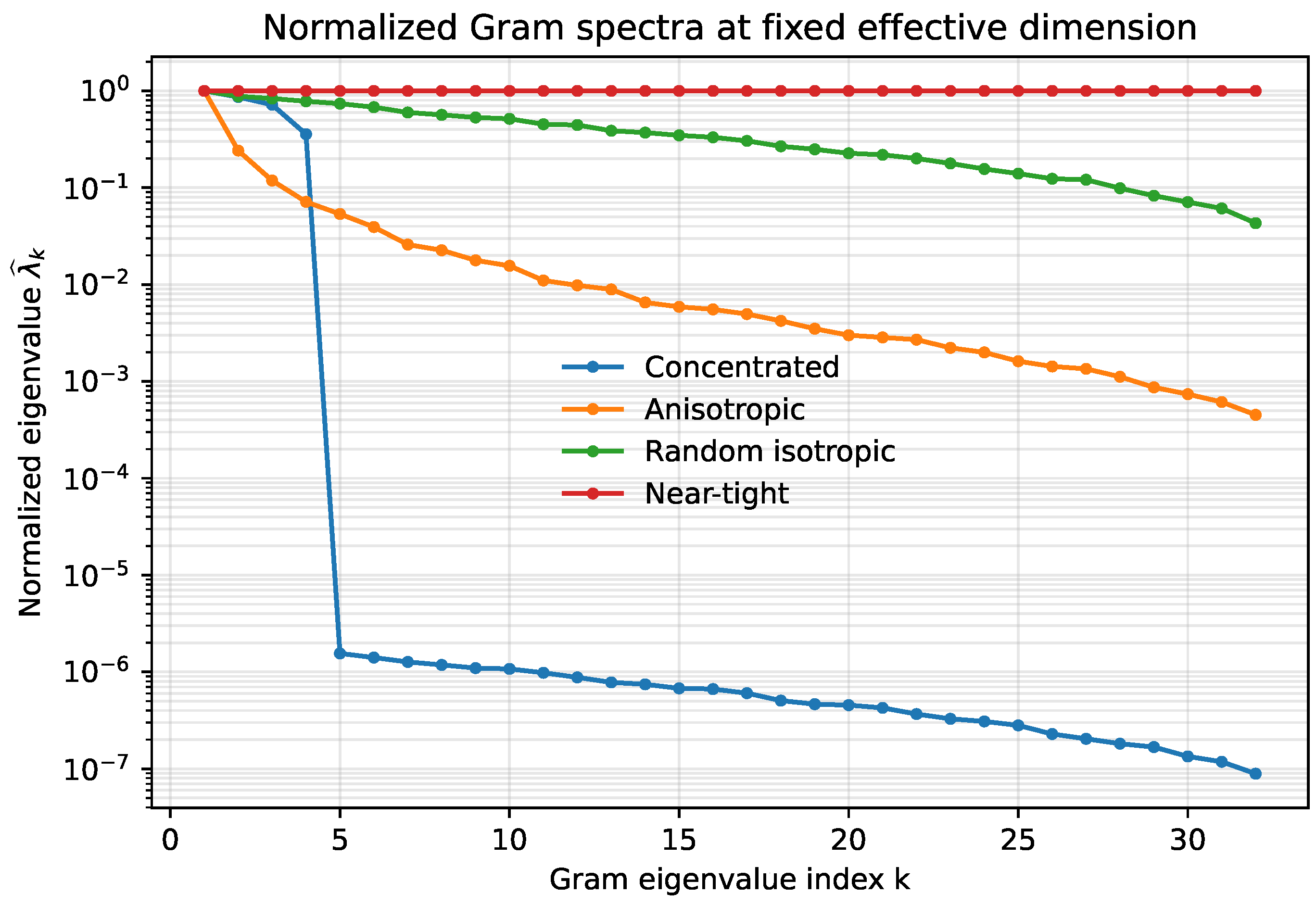
The first experiment isolates the role of measurement geometry. We take an effective operator space of dimension $n=dim\left(V\right)=32$ and compare four probing architectures with the same number of scalar measurements, $M=64,$ and the same total probing energy, $tr\left(G\right)=64.$ The four cases are:

• a concentrated probing family, whose probes are aligned with a small number of directions;
• an anisotropic probing family, which covers more directions but with a strongly decaying spectrum;
• a random isotropic probing family, which distributes sensitivity across all directions;
• a near-tight probing family, used as an ideal well-conditioned reference.

The purpose of this experiment is to show that the number of measurements and the effective dimension do not determine practical observability. What matters is the spectrum of the induced Gram operator.

Figure 1 shows the normalized Gram spectra. The four cases have the same measurement budget but very different visibility profiles. The concentrated architecture has only a few relevant eigenvalues. The anisotropic architecture has more nonzero directions, but many of them are weakly illuminated. The random isotropic architecture makes all directions visible at the reference threshold, although with nontrivial conditioning. The near-tight architecture gives the ideal flat spectrum.

The corresponding numerical values at ${\eta }_{\mathrm{ref}}={10}^{-2}$ are reported in

Table 1. Measurement-geometry experiment at fixed effective dimension $n=32$, fixed number of measurements $M=64$, and fixed total probing energy $tr\left(G\right)=64$. The observable dimension $N_{\mathrm{obs}}$ and observability condition number ${\kappa }_{\mathrm{obs}}$ are computed from the normalized Gram spectrum at the reference threshold ${\eta }_{\mathrm{ref}}={10}^{-2}$. Identical dimension and measurement budgets can therefore produce different observable dimensionalities and stability properties.

Architecture	${\mathit{N}}_{\mathbf{obs}}\left({10}^{-2}\right)$	${\mathit{\kappa }}_{\mathbf{obs}}\left({10}^{-2}\right)$
Concentrated	4	2.80
Anisotropic	11	90.72
Random isotropic	32	23.21
Near-tight	32	1.00

.

This experiment illustrates the distinction between algebraic dimensionality and practical observability. A large effective space may be available, and a large number of scalar measurements may be taken, but the resulting observable dimensionality depends on how the probing family embeds V into ${\mathbb{C}}^M$. Thus, $N_{\mathrm{obs}}\left(\eta \right)$ and ${\kappa }_{\mathrm{obs}}\left(\eta \right)$ capture information that is not contained in n, M, or $rank\left(G\right)$ alone.

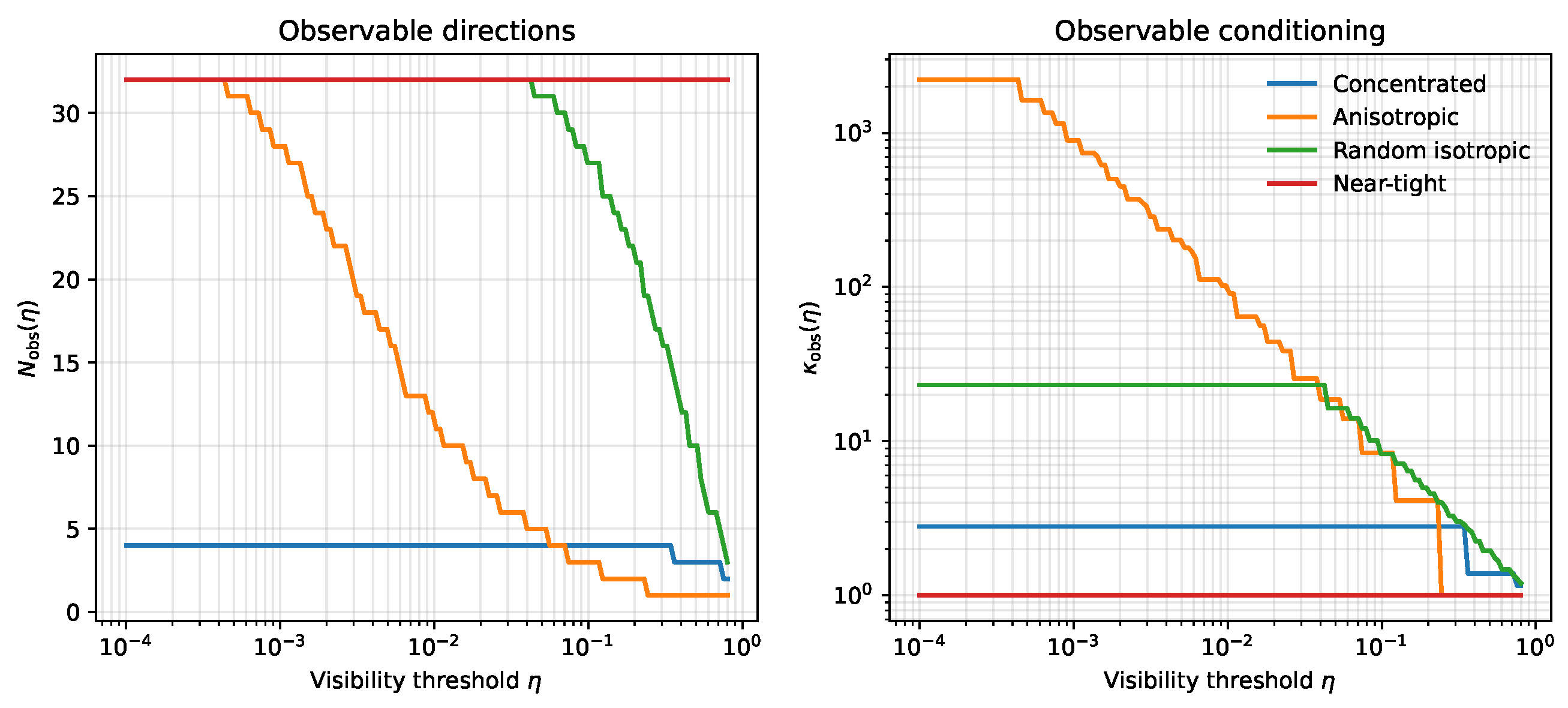
Figure 2 shows the dependence on the visibility threshold. This representation is useful because no single threshold is universal. A smaller threshold accepts weaker directions as observable, while a larger threshold retains only robustly visible directions. The condition-number curve shows the complementary stability information: a probing architecture may expose more directions only by admitting very weak eigenmodes, thereby increasing ${\kappa }_{\mathrm{obs}}\left(\eta \right)$.

6.2. Experiment 2: Symmetry-Induced Blindness

The second experiment illustrates the measurement-level meaning of the symmetry-resolved formulation of Section 4. We consider an effective operator space of dimension $n=32$, decomposed as an orthogonal direct sum of four sectors, $V=V_0\oplus V_1\oplus V_2\oplus V_3$, with $dim\left(V_{\alpha }\right)=8.$

The sector $V_0$ is interpreted as the invariant sector, while $V_1,V_2,V_3$ represent non-invariant sectors. The physical point of the experiment is not the particular choice of four sectors, but the fact that all sectors are present in $V_{\mathrm{eff}}$ while the probing architecture may illuminate only some of them. As in the previous experiment, all architectures are compared at fixed measurement budget and fixed probing-energy normalization, $M=64$, and $tr\left(G\right)=64$.

We compare three probing architectures:

• invariant-only probing, where all probes are contained in $V_0$;
• two-sector probing, where probes are distributed over $V_0\oplus V_1$;
• mixed probing, where probes are distributed over all four sectors.

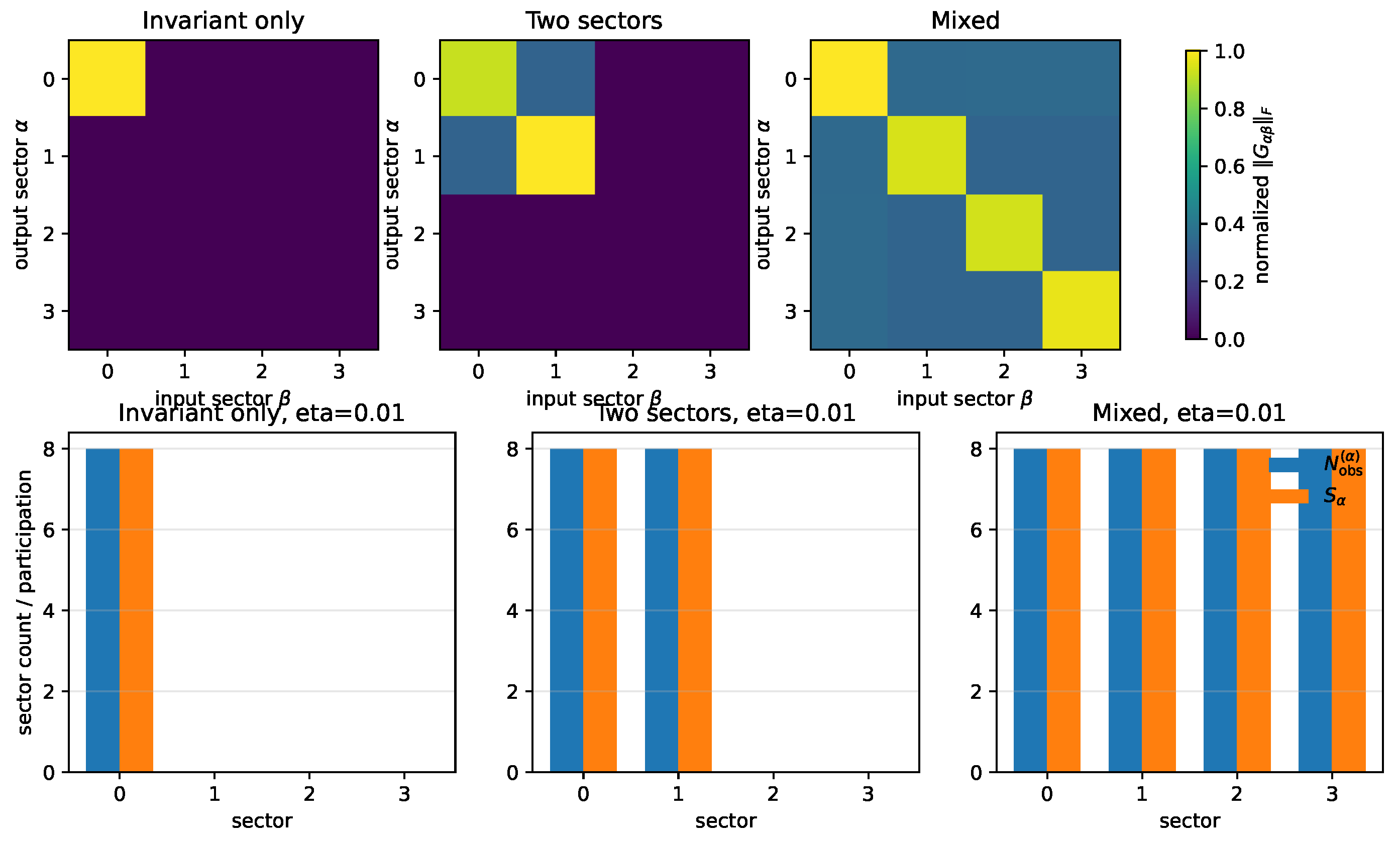
Let $P_{\alpha }$ denote the orthogonal projector onto $V_{\alpha }$. The sectorial Gram blocks are $G_{\alpha \beta }=P_{\alpha }G{P}_{\beta }.$ These blocks describe how the measurement geometry couples the sector decomposition. In the invariant-only case, every probe lies in $V_0$. Hence all non-invariant directions are orthogonal to all probes, and $V_1\oplus V_2\oplus V_3\subseteq ker\left(\mathcal{M}\right).$

This is the finite-dimensional numerical counterpart of Proposition 1: the non-invariant sectors may belong to the effective space and still be completely unobservable under an invariant probing architecture.

Figure 3 reports the Frobenius norms $\parallel G_{\alpha \beta }{\parallel }_F$. The invariant-only architecture produces energy only in the invariant block. The two-sector architecture activates the blocks associated with $V_0\oplus V_1$. The mixed architecture distributes probing energy across all sectors.

To avoid confusing sector-wise diagnostics with a decomposition of the full Gram spectrum, we report diagonal sector counts computed from the compressed operators $G_{\alpha }=P_{\alpha }G{P}_{\alpha }{|}_{V_{\alpha }}.$ At the reference threshold ${\eta }_{\mathrm{ref}}={10}^{-2}$, these compressed sector counts are

$$\begin{array}{cc}\mathrm{Architecture}& \left(N_{\mathrm{obs}}^{\left(0\right)},N_{\mathrm{obs}}^{\left(1\right)},N_{\mathrm{obs}}^{\left(2\right)},N_{\mathrm{obs}}^{\left(3\right)}\right)\\ \mathrm{Invariant}\mathrm{only}& (8,0,0,0)\\ \mathrm{Two}\sec \mathrm{tors}& (8,8,0,0)\\ \mathrm{Mixed}& (8,8,8,8).\end{array}$$

Here $N_{\mathrm{obs}}^{\left(\alpha \right)}$ is computed from the normalized spectrum of the compressed Gram $G_{\alpha }$, using the same visibility threshold as in the global observable-count definition.

These values should be interpreted as sector-wise compressed visibility indicators. When the Gram operator is block diagonal with respect to the sector decomposition, the corresponding sector counts add consistently. When off-diagonal blocks are present, the global observable dimension is determined by the full spectrum of G, and sector participation provides the appropriate description of how the visible eigendirections are distributed across the sectors. In all three cases, however, the qualitative conclusion is the same: symmetry-preserving probing can create genuine measurement nullspaces, while sectorially richer probing architectures redistribute sensitivity toward directions that were otherwise invisible.

6.3. Experiment 3: Controlled Symmetry Breaking

The third experiment tests the restricted visibility statement of Section 4.4. The purpose is to separate two effects that are easily conflated: the removal of exact blindness on the original nullspace and the appearance of practically observable directions in the normalized full Gram spectrum.

We start from a symmetric measurement architecture ${\mathcal{M}}_0$ with a nontrivial blind subspace $K_0=ker\left({\mathcal{M}}_0\right)$, and perturb it by

$${\mathcal{M}}_{\epsilon }={\mathcal{M}}_0+\epsilon {\mathcal{M}}_1,\epsilon \ge 0.$$

Let $G_{\epsilon }={\mathcal{M}}_{\epsilon }^{*}{\mathcal{M}}_{\epsilon }$, and let $P_0$ be the orthogonal projector onto $K_0$. On the original blind subspace, ${\mathcal{M}}_{0}x=0$ for every $x\in K_0$. Hence the compressed Gram operator satisfies

$$P_0{G}_{\epsilon }{P}_0={\epsilon }^2{P}_0{\mathcal{M}}_1^{*}{\mathcal{M}}_1{P}_0$$

as an operator on $K_0$. Equivalently, if $G_{\epsilon }^{\left(0\right)}=P_0{G}_{\epsilon }{P}_0{|}_{K_0}$, then the nonzero eigenvalues of $G_{\epsilon }^{\left(0\right)}$ must scale quadratically with $\epsilon$. This scaling test is performed on the compressed operator before any $\epsilon$-dependent trace renormalization of the full Gram matrix. The observable counts reported below are then evaluated from the normalized full Gram spectrum using the same convention and reference threshold as in the other experiments.

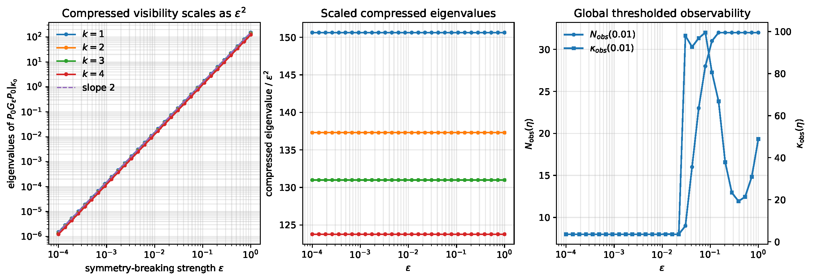
Figure 4 confirms the predicted restricted scaling. The estimated log–log slopes of the four leading compressed eigenvalues are all equal to $2.00$, up to the reported numerical precision. In other words, the compressed eigenvalues grow quadratically with the perturbation amplitude, as predicted by the symmetry-breaking argument.

In addition, the normalized diagnostic ${\lambda }_{max}\left(G_{\epsilon }^{\left(0\right)}\right)/{\epsilon }^2$ remains constant across the sweep, with numerical value approximately $150.64.$ These values verify the ${\epsilon }^2$ law on $K_0$ and identify the strength of the restricted visibility induced by ${\mathcal{M}}_1$.

The normalized full Gram spectrum shows a complementary effect. For small $\epsilon$, the originally blind directions acquire nonzero measurement energy, but their normalized eigenvalues remain below the reference threshold ${\eta }_{\mathrm{ref}}={10}^{-2}$. Consequently, the global observable count does not increase immediately. As the perturbation becomes stronger, those directions cross the threshold and the observable count rises from $N_{\mathrm{obs}}\left({10}^{-2}\right)=8$ to the full value $N_{\mathrm{obs}}\left({10}^{-2}\right)=32.$ Thus, controlled symmetry breaking removes exact algebraic blindness before it necessarily produces practical observability at a finite threshold.

This experiment supports the revised interpretation of the perturbative result. The theorem should not be read as a claim that a fixed number of eigenvalues of the full Gram spectrum automatically open in a useful way. Its precise content is that directions in the original blind subspace acquire compressed measurement energy at order ${\epsilon }^2$. Whether this energy becomes operationally observable depends on the normalized full spectrum, the chosen threshold, and the resulting conditioning.

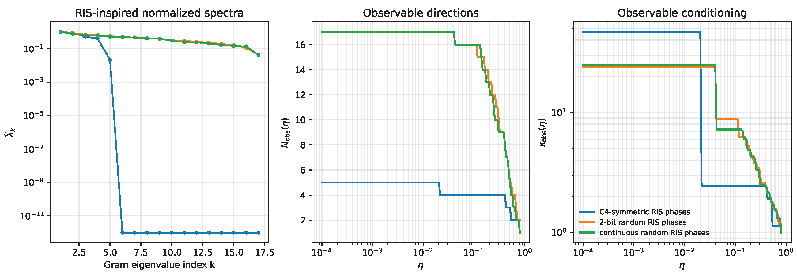
6.4. Experiment 4: RIS-Inspired Probing Architecture

The final experiment instantiates the proposed observability framework in a canonical narrowband RIS-assisted channel model. The purpose is not to provide a full-wave electromagnetic validation, but to show that the same Gram-based quantities used in the preceding abstract experiments can be computed for a familiar programmable-surface architecture.

We use the standard narrowband RIS-assisted effective-channel model introduced in Section 2.2. For the admissible RIS control family used in this experiment, the associated architecture-accessible space is the span of the effective channels generated by the admissible phase configurations. This space is induced by the chosen propagation model, transceiver dimensions, RIS states, and modelling resolution. It should not be confused with the number of RIS elements or with the number of admissible phase configurations.

This is the architecture-accessible space induced by the chosen propagation model, transceiver dimensions, RIS states, and modelling resolution. It should not be confused with the number of RIS elements or with the number of admissible phase configurations.

For the comparison below, a common effective space is first fixed from the RIS-inspired channel family at the chosen numerical resolution. In the reported experiment this space has dimension $n=dim\left(V_{\mathrm{eff}}\right)=17.$ The three probing architectures are then interpreted as different measurement designs on this same effective space. This avoids comparing different ambient dimensions and isolates the effect of the RIS phase-pattern geometry on the induced Gram spectrum.

Each scalar measurement has the form

$$y_m=w_m^{*}{H}_{\mathrm{eff}}\left({\varphi }_m\right)f_m,$$

where $f_m$ and $w_m$ are the transmit and receive configurations and ${\varphi }_m$ is the RIS phase pattern used in the m-th measurement. Equivalently, each measurement induces a linear functional on $V_{\mathrm{eff}}$. We compare three RIS phase families:

• $C_4$-symmetric RIS phase patterns;
• random 2-bit RIS phase patterns;
• continuous random RIS phase patterns.

All cases use the same number of scalar measurements, $M=64,$ and the same probing-energy normalization, $tr\left(G\right)=64.$ Thus, differences in $N_{\mathrm{obs}}\left(\eta \right)$ and ${\kappa }_{\mathrm{obs}}\left(\eta \right)$ are due to the geometry of the induced measurement family, not to different effective dimensions, different measurement budgets, or different total Gram energy. The channel model is the standard narrowband cascaded RIS form commonly used in RIS-assisted communication studies [5,6,7,8,9].

The normalized visibility spectra and the corresponding metrics are shown in Figure 5 and

Table 2. RIS-inspired experiment at fixed effective dimension $n=17$, fixed number of scalar measurements $M=64$, and fixed total probing energy $tr\left(G\right)=64$. The table reports the observable dimension $N_{\mathrm{obs}}$ and the observability condition number ${\kappa }_{\mathrm{obs}}$ at ${\eta }_{\mathrm{ref}}={10}^{-2}$. Symmetric RIS probing yields a smaller observable dimension and poorer conditioning, whereas random finite-resolution and continuous phase families recover full observable dimensionality at the prescribed threshold.

RIS Phase Family	${\mathit{N}}_{\mathbf{obs}}\left({10}^{-2}\right)$	${\mathit{\kappa }}_{\mathbf{obs}}\left({10}^{-2}\right)$
$C_4$-symmetric phases	5	46.71
2-bit random phases	17	23.75
Continuous random phases	17	24.63

. The $C_4$-symmetric phase family has the same effective dimension and measurement budget as the two randomized designs, but only

$$N_{\mathrm{obs}}\left({10}^{-2}\right)=5$$

effective directions remain visible at the reference threshold. This indicates that the symmetric probing family concentrates measurement sensitivity on a small subset of the effective operator space and leaves the remaining directions weakly represented. By contrast, both randomized phase families achieve

$$N_{\mathrm{obs}}\left({10}^{-2}\right)=17,$$

so all effective directions are visible at the same threshold. Their condition numbers are also better than that of the symmetric case, although they are not near-tight. This distinction is relevant: random RIS phases do not merely increase the observable count; they also produce a more balanced, but still imperfect, Gram spectrum.

This experiment provides the physical interpretation of the preceding abstract tests. It confirms that observable degrees of freedom are not determined solely by the number of effective operator directions, the number of scalar measurements, or the total probing energy. In a RIS-assisted setting, the phase-pattern family shapes the Gram geometry through which the effective channel space is observed. Highly symmetric phase patterns may be attractive for implementation or calibration, but they can also concentrate sensitivity and leave many effective directions below the visibility threshold. Randomized 2-bit patterns, despite their finite phase resolution, already provide enough diversity in this experiment to make the whole effective space visible at ${\eta }_{\mathrm{ref}}={10}^{-2}$. The relevant design objective is therefore not simply to enumerate admissible RIS states, but to choose probing families that distribute measurement sensitivity across the effective operator space while maintaining acceptable conditioning.

6.5. Summary of Numerical Findings

The four experiments support the measurement-geometric interpretation of observable degrees of freedom developed in the paper.

First, observable dimensionality is controlled by the normalized Gram spectrum rather than by the effective dimension or by the number of scalar measurements alone. At fixed n, fixed M, and fixed $tr\left(G\right)$, different probing geometries produce different values of $N_{\mathrm{obs}}\left(\eta \right)$ and ${\kappa }_{\mathrm{obs}}\left(\eta \right)$. Thus, the same measurement budget may yield either a low-dimensional, poorly distributed observation of $V_{\mathrm{eff}}$ or a stable embedding of the full effective space.

Second, symmetry can create genuine measurement nullspaces. Invariant probing illuminates the invariant sector but annihilates non-invariant sectors, even when those sectors belong to $V_{\mathrm{eff}}$. The sector-wise compressed Gram operators $G_{\alpha }=P_{\alpha }G{P}_{\alpha }{|}_{V_{\alpha }}$ provide useful diagnostics of direct sector visibility, while the full Gram spectrum remains the relevant object for global observable counts when sector coupling is present.

Third, controlled symmetry breaking produces the predicted second-order restricted visibility in the original blind subspace. The compressed eigenvalues on $K_0=ker\left({\mathcal{M}}_0\right)$ scale as ${\epsilon }^2$, whereas the global observable count increases only when the corresponding normalized eigenvalues exceed the prescribed threshold. This confirms the distinction between algebraic sensitivity and practical observability.

Fourth, the RIS-inspired experiment shows that the same framework can be instantiated in a canonical programmable-surface channel model. For a fixed effective operator space and a fixed measurement budget, symmetric RIS phase families may leave many effective directions below the visibility threshold, whereas random finite-resolution or continuous phase patterns can produce a flatter Gram spectrum and recover all effective directions at the chosen modelling resolution.

Overall, the experiments confirm the central message of the paper: physical and effective degrees of freedom describe what exists or can be accessed, whereas observable degrees of freedom describe what a finite, normalized, and physically constrained measurement architecture can distinguish stably.

7. Discussion

The objective of this work has been to separate three notions of dimensionality that are often conflated in programmable electromagnetic systems:

$$N_{\mathrm{obs}}\left(\eta \right)\le N_{\mathrm{eff}}\le N_{\mathrm{phys}}.$$

The physical layer describes the operator directions allowed by the propagation environment at the chosen modelling resolution. The effective layer describes the subset of those directions that remains accessible once a concrete architecture, hardware implementation, and signalling protocol are fixed. The observable layer is more restrictive: it contains only those effective directions that are distinguishable, at a prescribed resolution, by the finite measurement architecture actually used. The main point is that these three layers answer different operational questions. Physical admissibility does not imply architectural accessibility, and architectural accessibility does not imply stable observability.

This distinction is particularly important when the propagation system is not represented by a single fixed channel operator. Classical electromagnetic degrees-of-freedom analyses characterize the modal content of a given propagation realization, typically through singular spectra or spatial bandwidth arguments. In contrast, the present formulation uses finite-dimensional linear envelopes of admissible operator families. This does not mean that arbitrary linear combinations of physical configurations are themselves realizable. Rather, the span provides a common representation space in which variations of geometry, scattering conditions, frequency, relative motion, or other physical parameters can be compared. The corresponding effective space is then obtained by imposing architectural constraints, such as the implemented transmit and receive structures, available beams and combiners, hardware limitations, pilot resources, bandwidth, and admissible control states.

The measurement layer is the central addition of the paper. Once the effective operator space has been fixed, the finite probing family induces the measurement and observability Gram operators introduced in Section 3. The normalized spectrum of this Gram operator determines which effective directions are strongly visible, weakly visible, or effectively blind. The trace normalization fixes the total probing budget used to compare different architectures, while the normalized visibility spectrum defines a dimensionless threshold for observable degrees of freedom. Thus, $N_{\mathrm{obs}}\left(\eta \right)$ is not an algebraic rank alone: it is a finite-resolution count of effective operator directions whose measurement sensitivity exceeds the prescribed visibility level. The companion quantity ${\kappa }_{\mathrm{obs}}\left(\eta \right)$ records whether the visible subspace is well conditioned. This is the practical reason for using the Gram spectrum rather than only the number of measurements, the number of control states, or the dimension of $V_{\mathrm{eff}}$.

The role of frame theory in this formulation should be interpreted accordingly. The equivalence between stable embeddings, positive lower frame bounds, Gram spectra, and conditioning is standard. The contribution here is not a new abstract frame theorem, but the use of these tools to define an electromagnetic design quantity: the number of effective operator directions that remain distinguishable under a finite and physically constrained measurement architecture. This viewpoint makes it possible to compare probing schemes with the same effective dimension, the same number of measurements, and the same total probing energy, while still obtaining different observable dimensionalities and different stability properties.

The symmetry-resolved part of the paper adds a second interpretation layer. A decomposition of $V_{\mathrm{eff}}$ into symmetry sectors identifies how effective operator directions transform, but it does not by itself determine observability. What matters is the action of the Gram operator on and across those sectors. If the Gram operator is block diagonal, sectorial observable counts can be added consistently. If off-diagonal couplings are present, globally observable eigendirections may mix several sectors, and sector participation becomes the appropriate diagnostic. This distinction prevents a common overinterpretation: the existence of a sector is not the same as its measurement visibility.

Symmetry-induced blindness and controlled symmetry breaking are two consequences of this measurement-level view. Probing families confined to invariant sectors can leave non-invariant effective directions in the kernel of the measurement operator, even though those directions belong to $V_{\mathrm{eff}}$. Conversely, a symmetry-breaking perturbation can transfer measurement sensitivity to directions that were originally blind. The perturbative result in this paper is deliberately formulated on the compression of the perturbed Gram operator to the original blind subspace. It establishes second-order restricted visibility there, but it does not claim that the full Gram spectrum automatically develops well-conditioned observable eigenvalues. Whether newly exposed directions become useful depends on the normalized full spectrum, the visibility threshold, and the resulting conditioning.

The numerical experiments support this interpretation in controlled finite-dimensional settings. They show that fixed effective dimension, fixed number of scalar measurements, and fixed total probing energy do not determine $N_{\mathrm{obs}}\left(\eta \right)$ or ${\kappa }_{\mathrm{obs}}\left(\eta \right)$. These quantities depend on how measurement sensitivity is distributed across $V_{\mathrm{eff}}$. The experiments also illustrate that symmetric probing may create exact or effective blind subspaces, that compressed sector Grams are useful diagnostics but do not replace the global Gram spectrum, and that controlled symmetry breaking first produces restricted sensitivity on the original blind subspace before such directions necessarily become observable at a finite threshold. The RIS-inspired example shows that the same Gram-based quantities can be computed in a standard programmable-surface channel model, where different phase-pattern families acting on the same effective space produce different visibility spectra.

Several limitations should be noted. First, the framework is developed after a finite-dimensional modelling truncation. This is appropriate for finite arrays, finite RIS state sets, discretized channel models, and reduced operator representations, but it does not settle the corresponding infinite-dimensional theory. Second, the visibility threshold $\eta$ is application-dependent. It may be tied to noise level, calibration uncertainty, sample size, target estimation error, or numerical tolerance, but no universal value should be expected. Third, the RIS-inspired validation uses a canonical narrowband model rather than a full-wave electromagnetic solver. Its purpose is to demonstrate consistency with a familiar programmable-surface channel representation, not to provide hardware-level validation.

Despite these limitations, the framework suggests a concrete design principle. Programmable electromagnetic systems should not be assessed only by how many physical modes, control states, RIS elements, beams, pilots, or scalar measurements they possess. The relevant question for inference and control is whether the available probing architecture produces a sufficiently rich and well-conditioned measurement embedding of the effective operator space. In practical terms, this shifts part of the design problem toward shaping the Gram spectrum through pilot design, beam and combiner selection, RIS state scheduling, randomized probing, and controlled symmetry breaking. Observable degrees of freedom therefore provide a measurement-geometric complement to physical DoF, controllability, channel rank, and estimation error.

8. Conclusions

This paper has introduced an operator-space formulation of observable degrees of freedom for programmable electromagnetic environments. The central distinction is between three layers of dimensionality: physical degrees of freedom, associated with the family of propagation operators allowed by the electromagnetic environment; effective degrees of freedom, associated with the subset accessible to a concrete architecture; and observable degrees of freedom, associated with the part of the effective operator space that can be stably distinguished by a finite probing scheme.

Once the effective operator space has been fixed, observability is governed by the measurement operator and its associated Gram operator. Under a common probing-budget normalization, the normalized Gram spectrum provides a resolution-dependent description of visibility. The resulting quantities $N_{\mathrm{obs}}\left(\eta \right)$ and ${\kappa }_{\mathrm{obs}}\left(\eta \right)$ separate the number of visible operator directions from the conditioning with which those directions are measured. This distinction is important because architectures with the same effective dimension, the same number of scalar measurements, and the same total probing energy can induce substantially different observable subspaces and stability properties.

The symmetry-resolved part of the framework shows that sector decompositions do not determine observability by themselves. Sectorial directions may be strongly visible, weakly visible, or completely blind depending on how the probing family couples to the effective operator space. In particular, invariant probing can create exact nullspaces on non-invariant sectors, while controlled symmetry breaking redistributes measurement sensitivity toward directions that were originally blind. The relevant effect is therefore not the creation of additional physical modes, but the reshaping of the Gram geometry on the effective space.

The numerical experiments illustrate these mechanisms in controlled finite-dimensional settings and in a canonical RIS-inspired channel model. They show that observable dimensionality is not fixed by the number of accessible operator directions or by the number of measurements alone. Instead, it depends on how the probing architecture distributes measurement sensitivity across the effective operator space. Symmetric, anisotropic, randomized, and near-tight probing families can therefore lead to different values of $N_{\mathrm{obs}}\left(\eta \right)$ and ${\kappa }_{\mathrm{obs}}\left(\eta \right)$, even under identical measurement budgets.

The proposed framework should be understood as a measurement-geometric complement to electromagnetic degrees-of-freedom theory, RIS channel acquisition, frame-based sampling, and symmetry-resolved modal analysis. Its main design implication is that programmable electromagnetic systems should not be evaluated only by the number of physical modes, controllable parameters, RIS states, pilots, or beams. For inference, estimation, and control, the operational question is how many effective operator directions can be stably revealed by the measurements that the system can actually perform. Observable degrees of freedom provide a compact way to quantify this question and to turn Gram-spectrum shaping into an explicit design objective.