First Integral and General Solution of the Reduced Nonlinear Third-Order Differential Equation with a Nonlinear Source

Abstract

We consider a generalization of the modified Korteweg–de Vries–Burgers equation with a nonlinear source. Using the Painlevé test for partial differential equation with the Kruskal variable, we show that the corresponding Cauchy problem cannot be solved by the inverse scattering transform. However, the equation admits a two-wave solution, which is obtained by means of the Cole–Hopf transformation. Taking into account the traveling wave reduction, we derive the resulting nonlinear ordinary differential equation and determine the parameter conditions under which it passes the Painlevé test. This finding suggests the possible existence of the general solution for the ordinary differential equation, which can be reduced to the linear third-order equation. The general solution of the resulting linear equation is expressed in terms of the hypergeometric function.

1. Introduction

The study of high-order nonlinear partial differential equations plays a crucial role in describing various processes in modern mathematical physics. These equations often serve as fundamental models for wave propagation in dispersive and dissipative media, with applications spanning hydrodynamics, nonlinear optics, and plasma physics. Of particular interest are third-order nonlinear partial differential equations. A classic example is the well-known Korteweg–de Vries equation, which models surface waves in shallow water [1,2,3,4]. In such equations, the third-order derivative typically accounts for dispersive effects, while is combination with nonlinear terms can lead to the formation of solitons [5,6,7].

Currently, despite significant advances in the development of numerical methods and the qualitative theory of differential equations, the search for exact analytical solutions to nonlinear equations remains an important task [8,9,10,11,12,13]. Analytical solutions allow us to study various properties of mathematical models, such as the stability of the described processes and their asymptotic behavior [14,15,16,17,18,19,20]. Furthermore, they can be used to verify the accuracy of numerical algorithms.

Nonlinear partial differential equations (PDEs) can be classified as integrable or non-integrable. However, there are currently no general algorithms for constructing analytical solutions to nonlinear PDEs. For integrable equations, methods such as the inverse scattering transform (for solving Cauchy problems), the Bäcklund transformation (for generating exact solutions) [21,22,23,24,25,26,27,28], and the Hirota method (for constructing rational and soliton solutions) [29,30,31,32,33] are widely used.

For non-integrable nonlinear PDEs, researchers have a variety of special ansatz methods at their disposal to find analytical solutions [34,35,36,37,38,39,40]. A significant drawback of these approaches, however, is the inherent uncertainty in selecting an appropriate method for a given equation.

In our recent works [41,42,43], we have aimed to overcome this shortcoming by employing the following algorithm for constructing analytical solutions to nonlinear non-integrable PDEs. First, we apply the Painlevé test to determine the integrability properties of the original PDE [44,45,46,47,48,49,50]. This step helps assess whether analytical solutions are likely to exist.

Next, the analysis allows us to identify variables that reduce the original PDE to a nonlinear ordinary differential equation (ODE) and to find constraints on the equation’s parameters under which this ODE can admit an analytical solution. Additionally, testing the original equation for the Painlevé property often provides insight into the structure of the first integral for the resulting ODE. This insight can then be used to find either a general solution or a particular exact solution with fewer arbitrary constants.

The purpose of this work is to find exact analytical solutions to a nonlinear third-order partial differential equation of the form

$$\begin{array}{c}{u}_t+\beta u_{xxx}+\beta {\left(u^3\right)}_x+{\displaystyle \frac{3}{2}}\beta {\left(u^2\right)}_{xx}=\mu u_{xx}+\alpha u+\delta u^2-2\mu u^3.\end{array}$$

(1)

where $u(x,t)$ is a function of the independent variables x and t.

Equation (1) generalizes the well-known modified Korteweg–de Vries equation. The monomials with the second $u_{xx}$ and third derivatives $u_{xxx}$ in Equation (1) correspond to the dissipation and dispersion of disturbances in a nonlinear medium. The nonlinear terms with the first and second derivatives, namely $u^2{u}_x$ and ${\left(u^2\right)}_{xx}$, characterize nonlinear convection and dissipation. The nonlinear expressions on the right-hand side $\alpha u+\delta u^2-2\mu u^3$ are responsible for the friction and damping that occur during the propagation of a nonlinear wave. Additional explanations have been included in this version of the article. Moreover, the right-hand side of equation Equation (1) coincides with the Burgers–Huxley equation, which has been studied in many research papers. Therefore, Equation (1) can be considered as a natural generalization of the famous Burgers–Huxley models to the case of third derivatives and additional nonlinear expressions. To the best of our knowledge, Equation (1) is new and has not been studied previously.

The outline of this paper is as follows. In Section 2, we apply the Painlevé test to determine the integrability properties of Equation (1). We find that this equation is not integrable by the inverse scattering transform, as it fails the Painlevé test. Subsequently, in Section 3, we use the Cole–Hopf transformation to derive an exact solution of Equation (1). This procedure reduces Equation (1) to an overdetermined system of linear equations, which can be used to construct two-wave solutions. Finally, in Section 4, we present the general solution of Equation (1), expressed in terms of a hypergeometric function.

2. Application of the Painlevé Test to the Third-Order Differential Equation

The Painlevé test is one of the most powerful algorithms for verifying a necessary condition for the integrability of nonlinear differential equations. Currently, several algorithms exist for checking whether differential equations possess the Painlevé property. However, the simplest algorithm originates from the test used by S. V. Kovalevskaya in her analysis of the equations of motion for a rigid body with a fixed point [51,52].

This test was modernized in the works of Ablowitz, Ramani, and Segur into a procedure involving three sequential steps [48,49,50], a form in which it is now commonly applied. Initially, the algorithm was not used for nonlinear partial differential equations, but after the contributions of Weiss, Tabor, and Carnevale [53,54,55], it was widely adapted through the use of the Kruskal reduction.

We apply Painlevé test using the expansion of the solution of Equation (1) in the form

$$u(x,t)={\displaystyle \sum _{k=0}^{\infty }}{a}_k\left(t\right)F{(x,t)}^{k-p},$$

(2)

where $a_k\left(t\right)$ and $F(x,t)$ are new functions.

Using the first step of the Painlevé test and substituting $u=a_0\left(t\right)F^{-p}$ into the equation with the leading terms

$$\beta {\left(u^3\right)}_x+{\displaystyle \frac{3}{2}}\beta {\left(u^2\right)}_{xx}+\beta u_{xxx}=0,$$

(3)

we obtain two branches for the general solutions with values

$$(a_0^{\left(1\right)},p)=(1,1),(a_0^{\left(2\right)},p)=(2,1).$$

At the second step of the Painlevé test substituting the expression

$$u(x,t)=a_0\left(t\right)F{(x,t)}^{-1}+u_j{F}^{j-1}$$

into Equation (3), we obtain for the first branch the Fuchs indices in the form

$$j_1=-1,j_2=1,j_3=3.$$

(4)

For the second branch, we have the following Fuchs indices

$$j_1=-1,j_2=-2,j_3=3.$$

(5)

Substituting

$$u(x,t)=a_0\left(t\right)F^{-1}+a_1\left(t\right)+a_2\left(t\right)F+a_3\left(t\right)F^2+a_4\left(t\right)F^3+\dots$$

(6)

into Equation (1) and equating expressions at various powers of $F(x,t)=x-\psi \left(t\right)$ to zero, we obtain that the coefficient $a_1\left(t\right)$ can be taken as an arbitrary function of t, but the function $a_3\left(t\right)$ cannot be arbitrary because the compatibility the condition is not satisfied

$$K_3\left(t\right)=2\delta a_1\left(t\right)+{\displaystyle \frac{12{\mu }^2}{\beta }}{a}_1\left(t\right)+{\displaystyle \frac{2\mu }{\beta }}{\psi }_t+\alpha +{\displaystyle \frac{2\delta \mu }{\beta }}=0.$$

(7)

It is easy to see that $K_3\left(t\right)\ne 0$ in the general case. However, using the following constraints

$$\delta =-{\displaystyle \frac{6{\mu }^2}{\beta }},{\psi }_t=C_0={\displaystyle \frac{6{\mu }^2}{\beta }}-{\displaystyle \frac{\alpha \beta }{2\mu }}$$

(8)

we obtain $K_3\left(t\right)=0$.

In this case, we obtain the expansion for the first branch in the form

$$\begin{array}{c}u(x,t)={\displaystyle \frac{1}{F(x,t)}}+a_1\left(t\right)+\left({\displaystyle \frac{{\psi }_t}{3\beta }}+{\displaystyle \frac{\delta }{3\beta }}+{\displaystyle \frac{2\mu }{\beta }}{a}_2\left(t\right)-a_1{\left(t\right)}^2\right)F(x,t)+\\ +a_3\left(t\right)F{(x,t)}^2+\dots \end{array}$$

(9)

One can see from (8) and (9) that the first branch of the general solution passes the Painlevé test if we look for a solution taking into account the traveling wave reduction. The same results are obtained in the investigation of the second branch. Thus, we obtain that the partial differential equation does not pass the Painlevé test, and the Cauchy problem for Equation (1) cannot be solved by the inverse scattering transform. However, this suggests that a general solution may exist for the traveling wave reduction of Equation (1).

3. Exact Two-Wave Solutions of Partial Differential Equation

In this section, we obtain some exact solutions of Equation (1). First of all, let us introduce the operator $E_n\left[u\right]$ by the formula

$$E_n\left[u\right]={\left({\displaystyle \frac{\partial }{\partial x}}+u\right)}^{n}u.$$

(10)

The following two lemmas hold

Lemma 1.

If the function u is determined by the Cole–Hopf transformation

$$u={\displaystyle \frac{F_x}{F}},F=F(x,t),$$

(11)

then the following equality holds

$$\begin{array}{c}{E}_n\left[u\right]={\left({\displaystyle \frac{\partial }{\partial x}}+u\right)}^{n}u={\displaystyle \frac{F_{n+1,x}}{F}},F_{n+1,x}={\displaystyle \frac{{\partial }^{n+1}F(x,t)}{\partial x}}.\end{array}$$

(12)

Proof. 

The proof of the lemma is by induction. We have for $n=1$ the equality

$$\begin{array}{c}{E}_1\left[u\right]=u_x+u^2={\displaystyle \frac{F_{xx}}{F}}.\end{array}$$

(13)

We assume that the following equality holds

$$\begin{array}{c}{E}_{m-1}\left[u\right]={\left({\displaystyle \frac{\partial }{\partial x}}+u\right)}^{m}u={\displaystyle \frac{F_{m,x}}{F}}.\end{array}$$

(14)

Let us consider the following chain of equalities

$$\begin{array}{c}{E}_m\left[u\right]=\left({\displaystyle \frac{\partial }{\partial x}}+u\right){\left({\displaystyle \frac{\partial }{\partial x}}+u\right)}^{m}u=\left({\displaystyle \frac{\partial }{\partial x}}+u\right)E_{m-1}\left[u\right]=\\ =\left({\displaystyle \frac{\partial }{\partial x}}+u\right){\displaystyle \frac{F_{m,x}}{F}}={\displaystyle \frac{F_{m+1,x}}{F}}.\end{array}$$

(15)

This concludes the proof of the lemma. □

Taking into account the operator (10), we present Equation (1) in the form

$$\begin{array}{c}{u}_t+\alpha E_0-\mu E_2+\beta E_3+u(\delta E_0+3\mu E_1-\beta E_2)=0.\end{array}$$

(16)

Theorem 1.

If a solution $u(x,t)$ of Equation (1) is looked for using the Cole–Hopf transformation, then function $F(x,t)$ satisfies the following system of equations

$$\begin{array}{c}{F}_{xt}+\alpha F_x+3\mu F_{xxx}-\beta F_{xxxx}=0,\end{array}$$

(17)

$$\begin{array}{c}\delta F_x+3\mu F_{xx}-\beta F_{xxx}-F_t=0.\end{array}$$

(18)

Proof. 

Substituting u and $E_k,k=0,1,2,3$ into Equation (16) and equating expressions corresponding to powers of $F(x,t)$ to zero, we obtain Equations (17) and (18). □

From Equation (18), we have

$$F_t=\delta F_x+3\mu F_{xx}-\beta F_{xxx}.$$

(19)

Substituting Equation (19) into Equation (18), we obtain

$$\alpha F_x+\delta F_{xx}+2\mu F_{xxx}=0.$$

(20)

The solution of Equation (20) can be written in the form

$$F(x,t)=C_1\left(t\right)+C_2\left(t\right){\mathrm{e}}^{p_{1}x}+C_3\left(t\right){\mathrm{e}}^{p_{2}x},$$

(21)

where $C_1$ is an arbitrary function of t and $p_k(k=1,2)$ are the roots of the quadratic equation

$$\alpha +\delta p+2\mu p^2=0.$$

(22)

The functions $C_k\left(t\right)$ are determined by substituting Equation (21) into Equation (18) and equating the coefficients of the exponent terms to zero. This yields the following functions

$$\begin{array}{c}{C}_1\left(t\right)=C_1,C_1\left(t\right)=C_1^{\left(0\right)}{\mathrm{e}}^{p_1(\delta +3\mu p_1-\beta p_1^2)t},\\ C_2\left(t\right)=C_2^{\left(0\right)}{\mathrm{e}}^{p_1(\delta +3\mu p_1-\beta p_1^2)t},\end{array}$$

(23)

where $C_1^{\left(0\right)}$ and $C_2^{\left(0\right)}$ are arbitrary constants and $p_{1,2}$

$$\begin{array}{c}{p}_{1,2}={\displaystyle \frac{-\delta \pm \sqrt{\delta -8\mu \alpha }}{4\mu }}.\end{array}$$

(24)

Exact solution $F(x,t)$ takes the form

$$\begin{array}{c}F(x,t)=C_1+exp\left\{p_1\left[(x-x_1)-(\delta +3\mu p_1+\beta p_1^2)t\right]\right\}+\\ +exp\left\{p_2\left[(x-x_2)-(\delta +3\mu p_2+\beta p_2^2)t\right]\right\},\end{array}$$

(25)

where $x_1$ and $x_2$ are arbitrary constants that are determined by the constants $C_2^{\left(0\right)}$ and $C_3^{\left(9\right)}$.

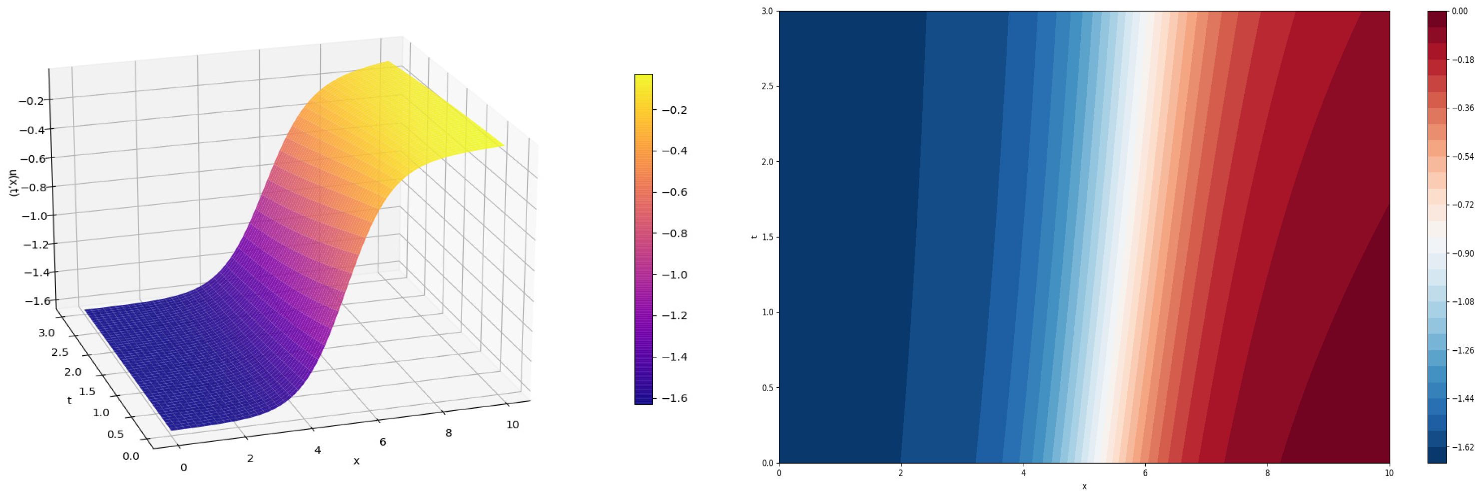
Substituting (25) into formula (11), we obtain the two-wave solution of Equation (1).

Figure 1 demonstrates solution (11) of the wave (left) and heat map (right) at $\alpha =0.1$, $\beta =0.3$, $\delta =0.2$, $\mu =0.5$, $C_1=0.5$, $x_1=1.0$ and $x_2=5.0$.

4. The First Integral and General Solution of the Reduced Differential Equation

We look for a solution of Equation (1) using the traveling wave reduction

$$\begin{array}{c}u(x,t)=y\left(z\right),z=x-C_{0}t.\end{array}$$

(26)

Substituting (26) into Equation (1), we obtain a nonlinear ordinary differential equation in the form

$$\begin{array}{c}\beta y_{zzz}+3\beta y^2{y}_z+{\displaystyle \frac{3}{2}}\beta {\left(y^2\right)}_{zz}-\mu y_{zz}-C_0{y}_z+\alpha y+\delta y^2+2\mu y^3=0.\end{array}$$

(27)

Using the conditions (8) of the Painlevé test, we look for the general solution of a special case of Equation (27) in the following form

$$\begin{array}{c}\beta y_{zzz}+3\beta y^2{y}_z+{\displaystyle \frac{3}{2}}\beta {\left(y^2\right)}_{zz}-\mu y_{zz}-\left({\displaystyle \frac{6{\mu }^2}{\beta }}-{\displaystyle \frac{\alpha \beta }{2\mu }}\right)y_z+\\ +\alpha y-{\displaystyle \frac{6{\mu }^2}{\beta }}{y}^2+2\mu y^3=0.\end{array}$$

(28)

In order to find the general solution of Equation (28), we determine the first integral corresponding to the arbitrary function $a_3\left(t\right)$. Using the polynomial with unknown coefficients in the form

$$\begin{array}{c}P=A_0{y}_{zz}+A_{1}y{y}_z+A_2{y}_z+A_3{y}^3+A_4{y}^2+A_5.\end{array}$$

(29)

Substituting (29) and $y_{zzz}$ from Equation (28) into the equation

$$\begin{array}{c}{P}_z-mP=0,\end{array}$$

(30)

we find that coefficients $A_k,(k=1,2,\dots ,5)$ and the parameter m can be determined.

They take the form

$$\begin{array}{c}{A}_1=3A_0,A_2=\left(m-{\displaystyle \frac{\mu }{\beta }}\right)A_0,A_3=A_4,A_4={\displaystyle \frac{3m}{2}}{A}_0,\\ A_5=\left(m^2-{\displaystyle \frac{\mu m}{\beta }}+{\displaystyle \frac{\alpha }{2\mu }}-6{\displaystyle \frac{{\mu }^2}{{\beta }^2}}\right)A_0,m=-{\displaystyle \frac{2\mu }{\beta }}.\end{array}$$

(31)

Taking into account Equations (29) and (30) and assuming $A_0=1$, we obtain the first integral of Equation (28) as follows

$$\begin{array}{c}{y}_{zz}+3y{y}_z-{\displaystyle \frac{3\mu }{\beta }}{y}_z+y^3-{\displaystyle \frac{3\mu }{\beta }}{y}^2+{\displaystyle \frac{\alpha }{2\mu }}y=C_{4}exp\left(-{\displaystyle \frac{2\mu }{\beta }}z\right),\end{array}$$

(32)

where $C_4$ is an arbitrary constant.

Using the transformation of the form

$$\begin{array}{c}y\left(z\right)={\displaystyle \frac{V_z}{V}},V=V\left(z\right),\end{array}$$

(33)

we reduce Equation (32) to a linear ordinary differential equation of the third order

$$\begin{array}{c}{V}_{zzz}-{\displaystyle \frac{3\mu }{\beta }}{V}_{zz}+{\displaystyle \frac{\alpha }{2\mu }}{V}_z-V{C}_{4}exp\left(-{\displaystyle \frac{2\mu }{\beta }}z\right)=0.\end{array}$$

(34)

The general solution of Equation (34) is expressed in terms of the hypergeometric function in the form

$$\begin{array}{c}V\left(z\right)=C_5{}_{0}F_2\left(\left[\right],\left[{\displaystyle \frac{7{\mu }^2+\sqrt{\mu }S}{4{\mu }^2}},{\displaystyle \frac{\alpha {\beta }^2-{\mu }^3+3{\mu }^{3/2}S}{2\mu ({\mu }^2+\sqrt{\mu }S)}}\right],-{\displaystyle \frac{C_4{\beta }^2}{8{\mu }^3}}{\mathrm{e}}^{-{\displaystyle \frac{2\mu }{\beta }}z}\right)+\\ C_{6}exp\left({\displaystyle \frac{6{\mu }^3-\alpha {\beta }^2+2{\mu }^{3/2}S}{({\mu }^2+\sqrt{\mu }S)\beta }}z\right)+\\ {}_{0}F_2\left(\left[\right],\left[-{\displaystyle \frac{\sqrt{\mu }S-{\mu }^2}{4{\mu }^2}},{\displaystyle \frac{2\alpha {\beta }^2-7{\mu }^3+{\mu }^{3/2}S}{2\mu ({\mu }^2+\sqrt{\mu }S)}}\right],-{\displaystyle \frac{C_4{\beta }^3}{8{\mu }^3}}{\mathrm{e}}^{-{\displaystyle \frac{2\mu }{\beta }}z}\right)+\\ C_{7}exp\left({\displaystyle \frac{\alpha {\beta }^2-3{\mu }^3+{\mu }^{3/2}S}{({\mu }^2+\sqrt{\mu }S)\beta }}z\right)+\\ {}_{0}F_2\left(\left[\right],\left[-{\displaystyle \frac{5{\mu }^3-\alpha {\beta }^2+{\mu }^{3/2}S}{2\mu ({\mu }^2+\sqrt{\mu }S)}},{\displaystyle \frac{11{\mu }^3-2\alpha {\beta }^2+3{\mu }^{3/2}S}{2\mu ({\mu }^2+\sqrt{\mu }S)}}\right],-{\displaystyle \frac{C_4{\beta }^3}{8{\mu }^3}}{\mathrm{e}}^{-{\displaystyle \frac{2\mu }{\beta }}z}\right),\end{array}$$

(35)

where ${}_{0}F_2\left([,],[,],\xi \right)$ is a hypergeometric function and the parameter S is introduced by the formula:

$$S=\sqrt{9{\mu }^3-2\alpha {\beta }^2}.$$

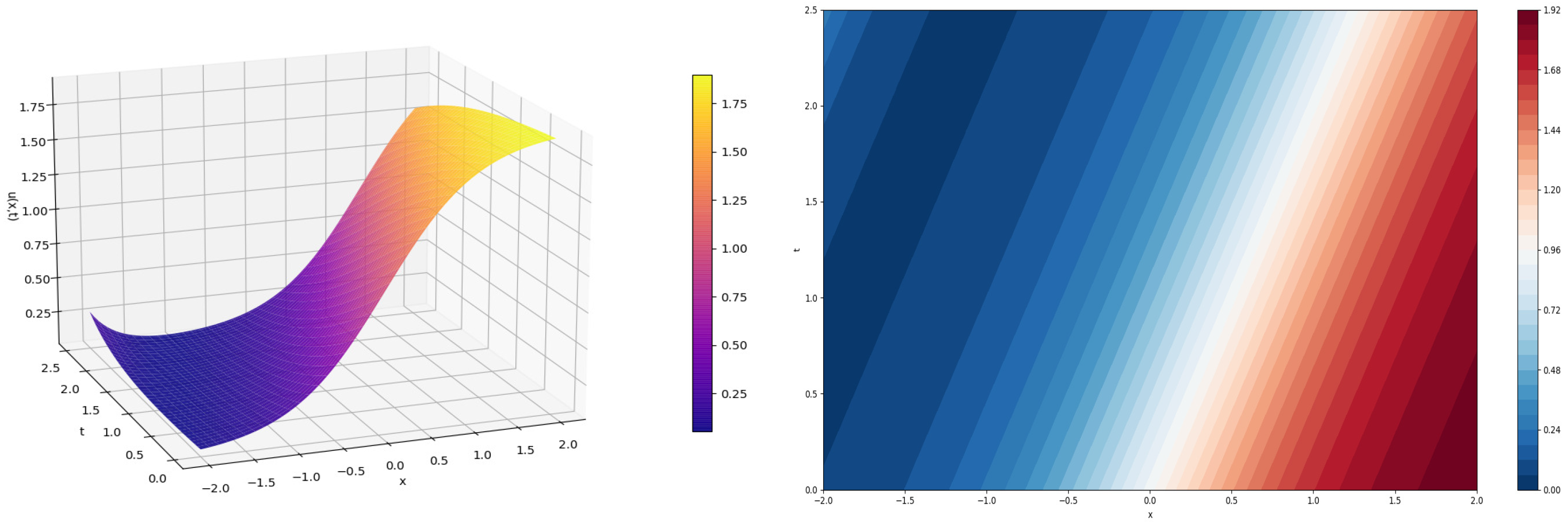
The general solution of Equation (28) is determined by formula (33). This solution contains three arbitrary constants.

Assuming $C_4=0$, we obtain a linear third-order ordinary differential equation in the form

$$\begin{array}{c}{V}_{zzz}-{\displaystyle \frac{3\mu }{\beta }}{V}_{zz}+{\displaystyle \frac{\alpha }{2\mu }}{V}_z=0.\end{array}$$

(36)

The solution of Equation (36) is given by

$$\begin{array}{c}V\left(z\right)=C_8+C_{9}exp\left({\lambda }_{1}z\right)+C_{10}exp\left({\lambda }_{2}z\right),\end{array}$$

(37)

where $C_8$, $C_9$, and $C_{10}$ are arbitrary constants, and ${\lambda }_{1,2}$ are determined by the formula

$$\begin{array}{c}{\lambda }_{1,2}={\displaystyle \frac{3{\mu }^2\pm \sqrt{9{\mu }^4-2\mu \alpha {\beta }^2}}{2\mu \beta }}\end{array}$$

(38)

We obtain an exact solution of Equation (27) by taking into account solution (37) and conditions (8). This exact solution is similar to, but not identical with, the solution given by Equation (25).

Figure 2 demonstrates solution (33) of the wave (left) and heat map (right) at $\alpha =0.1$, $\beta =0.3$, $\delta =2.0$, $\mu =1.0$, $C_0=0.5$, $C-4=0.01$, $C_5=0.3$, $C_6=2.0$ and $C_7=2.0$.

5. Conclusions

This article investigates a nonlinear third-order equation that generalizes the modified Korteweg–de Vries–Burgers equation, incorporating nonlinear dissipation and a nonlinear source. The Painlevé test is applied to study the integrability of this nonlinear partial differential equation. It is shown that the Cauchy problem for the considered equation is not solved by the inverse scattering transform, since the equation fails the Painlevé test. However, the application of the Cole–Hopf transformation allows the original equation to be rewritten as a linear overdetermined system, with two wave solutions. It is established that the corresponding nonlinear ordinary differential equation passes the Painlevé test. Using insights obtained from this test, we derive a non-autonomous first integral for the differential equation, which can be reduced to a linear equation. The general solution of this linear equation is expressed in terms of a hypergeometric function.

References

1. Korteweg, D.J.; de Vries, G. On the Change of Form of Long Waves Advancing in a Rectangular Canal and on a New Type of Long Stationary Wave. Philos. Mag. 1895, 39, 422–443. [Google Scholar] [CrossRef]
2. Russell, J.S. Report on Waves. In Report of the 14th Meeting of the British Association for the Advancement of Science; John Murray: York, UK, 1844; pp. 311–390. [Google Scholar]
3. Drazin, P.G. Nonlinear Systems; Cambridge University Press: Cambridge, UK, 1992. [Google Scholar]
4. Ablowitz, M.J.; Clarkson, P.A. Solitons, Nonlinear Evolution Equations and Inverse Scattering; Cambridge University Press: Cambridge, UK, 1991. [Google Scholar]
5. Drazin, P.G.; Johnson, R.S. Solitons: An Introduction; Cambridge University Press: Cambridge, UK, 1989. [Google Scholar]
6. Zabusky, N.J.; Kruskal, M.D. Interaction of “Solitons” in a Collisionless Plasma and the Recurrence of Initial States. Phys. Rev. Lett. 1965, 15, 240–243. [Google Scholar] [CrossRef]
7. Gardner, C.S.; Greene, J.M.; Kruskal, M.D.; Miura, R.M. Method for Solving the Korteweg-deVries Equation. Phys. Rev. Lett. 1967, 19, 1095–1097. [Google Scholar] [CrossRef]
8. Kudryashov, N.A. Exact Solutions of the Generalized Kuramoto-Sivashinsky Equation. Phys. Lett. A 1990, 147, 287–291. [Google Scholar] [CrossRef]
9. Shah, R.; Khan, H.; Baleanu, D.I.; Kumam, P.; Arif, M.U. A Semi-Analytical Method to Solve Family of Kuramoto-Sivashinsky Equations. J. Taibah Univ. Sci. 2020, 14, 402–411. [Google Scholar] [CrossRef]
10. Vitanov, N.K.; Dimitrova, Z.I.; Kantz, H. Modified Method of Simplest Equation and Its Application to Nonlinear PDEs. Appl. Math. Comput. 2010, 216, 2587–2595. [Google Scholar] [CrossRef]
11. Sahoo, S.; Ray, S.S. New Approach to Find Exact Solutions of Time-Fractional Kuramoto-Sivashinsky Equation. Phys. A 2015, 434, 240–245. [Google Scholar] [CrossRef]
12. Kilicman, A.; Silambarasan, R. Modified Kudryashov Method to Solve Generalized Kuramoto-Sivashinsky Equation. Symmetry 2018, 10, 527. [Google Scholar] [CrossRef]
13. Jaradat, H.M.; Alquran, M.T.; Syam, M.I. A Reliable Study of New Nonlinear Equation: Two-Mode Kuramoto-Sivashinsky. Int. J. Appl. Comput. Math. 2018, 4, 64. [Google Scholar] [CrossRef]
14. Kawahara, T. Formation of Saturated Solitons in a Nonlinear Dispersive System with Instability and Dissipation. Phys. Rev. Lett. 1983, 51, 381–383. [Google Scholar] [CrossRef]
15. Topper, J.; Kawahara, T. Approximate Equations for Long Nonlinear Waves on a Viscous Fluid. J. Phys. Soc. Jpn. 1978, 44, 663–666. [Google Scholar] [CrossRef]
16. Kawahara, T. Derivative-Expansion Method for Nonlinear Waves on a Liquid Layer of Slowly Varying Depth. J. Phys. Soc. Jpn. 1975, 38, 1200–1206. [Google Scholar] [CrossRef]
17. Sivashinsky, G.I. On a Distorted Flame Front as a Hydrodynamic Discontinuity. Acta Astronaut. 1977, 3, 889–918. [Google Scholar]
18. Sivashinsky, G.I. Nonlinear Analysis of Hydrodynamic Instability in Laminar Flames—I. Derivation of Basic Equations. Acta Astronaut. 1977, 4, 1177–1206. [Google Scholar] [CrossRef]
19. Kuramoto, Y.; Tsuzuki, T. On the Formation of Dissipative Structures in Reaction-Diffusion Systems. Prog. Theor. Phys. 1975, 54, 687–699. [Google Scholar] [CrossRef]
20. Cohen, B.I.; Krommes, J.A.; Tang, W.M.; Rosenbluth, M.N. Non-Linear Saturation of the Dissipative Trapped-Ion Mode by Mode Coupling. Nucl. Fusion 1976, 16, 971–992. [Google Scholar] [CrossRef]
21. Weiss, J. Bäcklund Transformation and Linearizations of the Hénon–Heiles System. Phys. Lett. A 1984, 102, 329–331. [Google Scholar] [CrossRef]
22. Gao, N.-N.; Fan, F.-C. The Focusing and Defocusing Fifth-Order Semi-Discrete mKdV Equation: Bäcklund Transformation, Soliton Solution and Continuous Limit. Rep. Math. Phys. 2026, 97, 201–218. [Google Scholar] [CrossRef]
23. Raza, N.; Kaplan, M.; Jannat, N.; Akbulut, A.; Muhammad, T. Nonlinear Wave Dynamics: Soliton and Complexiton Solutions of the Generalized Shallow-Water-Like Equation in Coastal and Plasma Physics. Indian J. Phys. 2026, 100, 1593–1603. [Google Scholar] [CrossRef]
24. Gai, L.; Chen, Y.; Wu, W. Bäcklund Transformation, N-Solitons and Standardized Analyses of Novel Waves for a (2+1)-Dimensional Extended Kadomtsev-Petviashvili Equation. Nonlinear Dyn. 2026, 114, 12438. [Google Scholar] [CrossRef]
25. Ozisik, M.; Secer, A.; Bayram, M. Obtaining Analytical Solutions of (2+1)-Dimensional Nonlinear Zoomeron Equation by Using Modified F-Expansion and Modified Generalized Kudryashov Methods. Eng. Comput. 2024, 41, 1105–1120. [Google Scholar] [CrossRef]
26. Ozisik, M.; Secer, A.; Bayram, M. On the Investigation of Chiral Solitons via Modified New Kudryashov Method. Int. J. Geom. Methods Mod. Phys. 2023, 20, 2350117. [Google Scholar] [CrossRef]
27. Ozisik, M.; Secer, A.; Bayram, M.; Sulaiman, T.A.; Yusuf, A. Acquiring the Solitons of Inhomogeneous Murnaghan’s Rod Using Extended Kudryashov Method with Bernoulli-Riccati Approach. Int. J. Mod. Phys. B 2022, 36, 2250221. [Google Scholar] [CrossRef]
28. Ekici, M. Exact Solutions to Some Nonlinear Time-Fractional Evolution Equations Using the Generalized Kudryashov Method in Mathematical Physics. Symmetry 2023, 15, 1961. [Google Scholar] [CrossRef]
29. Ali, A.; Hassan, A.U.; Rizvi, S.T.R. Granular Chain Wave Dynamics Under Hertz Nonlinearity via a Hybrid Hirota-Based Bilinear Neural Network. Chaos Solitons Fractals 2026, 208, 118306. [Google Scholar] [CrossRef]
30. Althobaiti, A.; Malik, S.; Alsharif, F.; Murad, M.A.S.; Mandal, U.K. Exploring Wronskian, Soliton, Lump and Lump-Multi-Kink Solutions of a (3+1)-Dimensional Boussinesq Type Equation Using Hirota Bilinear and Riccati Methods. Pramana 2026, 100, 3117. [Google Scholar] [CrossRef]
31. Fan, E.; Hon, Y.C. Quasiperiodic Waves and Asymptotic Behavior for Bogoyavlenskii’s Breaking Soliton Equation in (2+1) Dimensions. Phys. Rev. E 2008, 78, 036607. [Google Scholar] [CrossRef] [PubMed]
32. Kumar, S.; Mohan, B.; Kumar, R. Lump, Soliton, and Interaction Solutions to a Generalized Two-Mode Higher-Order Nonlinear Evolution Equation in Plasma Physics. Nonlinear Dyn. 2022, 110, 693–704. [Google Scholar] [CrossRef]
33. Wazwaz, A.-M. The Hirota’s Direct Method and the Tanh-Coth Method for Multiple-Soliton Solutions of the Sawada-Kotera-Ito Seventh-Order Equation. Appl. Math. Comput. 2008, 199, 133–138. [Google Scholar] [CrossRef]
34. Kudryashov, N.A. Simplest Equation Method to Look for Exact Solutions of Nonlinear Differential Equations. Chaos Solitons Fractals 2005, 24, 1217–1231. [Google Scholar] [CrossRef]
35. Kudryashov, N.A. One Method for Finding Exact Solutions of Nonlinear Differential Equations. Commun. Nonlinear Sci. Numer. Simul. 2012, 17, 2248–2253. [Google Scholar] [CrossRef]
36. Khalique, C.M. Solutions of a Generalized Complexly Coupled Korteweg-de Vries System Using Simplest Equation Method. In Proceedings of the 2014 International Conference on Computational Science and Computational Intelligence (CSCI), Las Vegas, NV, USA, 10–13 March 2014; Volume 2, pp. 223–225. [Google Scholar] [CrossRef]
37. Aziz, T.; Fatima, A.; Khalique, C.M.; Mahomed, F.M. Prandtl’s Boundary Layer Equation for Two-Dimensional Flow: Exact Solutions via the Simplest Equation Method. Math. Probl. Eng. 2013, 2013, 724385. [Google Scholar] [CrossRef]
38. Vitanov, N.K.; Dimitrova, Z.I. Modified Method of Simplest Equation Applied to the Nonlinear Schrödinger Equation. J. Theor. Appl. Mech. 2018, 48, 59–68. [Google Scholar] [CrossRef]
39. Vitanov, N.K.; Dimitrova, Z.I.; Vitanov, K.N. Modified Method of Simplest Equation for Obtaining Exact Analytical Solutions of Nonlinear Partial Differential Equations: Further Development of the Methodology with Applications. Appl. Math. Comput. 2015, 269, 363–378. [Google Scholar] [CrossRef]
40. Mahmood, S.S.; Murad, M.A.S. Optical Solutions of Weakly Nonlocal Media for Nonlinear Conformable Schrödinger Equation by Extended Simplest Equation Method. Phys. Lett. A 2025, 560, 130936. [Google Scholar] [CrossRef]
41. Kudryashov, N.A. Painlevé Analysis of the Resonant Third-Order Nonlinear Schrödinger Equation. Appl. Math. Lett. 2024, 158, 109232. [Google Scholar] [CrossRef]
42. Kudryashov, N.A. Painlevé Analysis of the Sasa–Satsuma Equation. Phys. Lett. A 2024, 525, 129900. [Google Scholar] [CrossRef]
43. Kudryashov, N.A. Painlevé Test, First Integrals and Analytical Solutions of the Korteweg-de Vries-Burgers Equation with a Nonlinear Source. Chaos Solitons Fractals 2025, 201, 117380. [Google Scholar] [CrossRef]
44. Painlevé, P. Sur les Équations Différentielles du Second Ordre à Points Critiques Fixes. C. R. Acad. Sci. Paris 1898, 126, 1697–1700. [Google Scholar]
45. Painlevé, P. Mémoire sur les Équations Différentielles Dont l’Intégrale Générale Est Uniforme. Bull. Soc. Math. Fr. 1900, 28, 201–261. [Google Scholar]
46. Painlevé, P. Sur les Équations Différentielles du Second Ordre et d’Ordre Supérieur Dont l’Intégrale Générale Est Uniforme. Acta Math. 1902, 25, 1–85. [Google Scholar]
47. Painlevé, P. Sur les Équations Différentielles du Second Ordre à Points Critiques Fixes. C. R. Acad. Sci. Paris 1906, 143, 1111–1117. [Google Scholar]
48. Ablowitz, M.J.; Ramani, A.; Segur, H. A Connection Between Nonlinear Evolution Equations and Ordinary Differential Equations of P-Type. I. J. Math. Phys. 1980, 21, 715–721. [Google Scholar] [CrossRef]
49. Ablowitz, M.J.; Ramani, A.; Segur, H. Nonlinear Evolution Equations and Ordinary Differential Equations of Painlevé Type. Lett. Nuovo Cimento 1978, 23, 333–338. [Google Scholar] [CrossRef]
50. Ablowitz, M.J.; Ramani, A.; Segur, H. A Connection Between Nonlinear Evolution Equations and Ordinary Differential Equations of P-Type. II. J. Math. Phys. 1980, 21, 1006–1015. [Google Scholar] [CrossRef]
51. Kowalevski, S. Sur le Problème de la Rotation d’un Corps Solide Autour d’un Point Fixe. Acta Math. 1889, 12, 177–232. [Google Scholar] [CrossRef]
52. Kowalevski, S. Sur une Propriété du Système d’Équations Différentielles qui Définit la Rotation d’un Corps Solide Autour d’un Point Fixe. Acta Math. 1890, 14, 81–93. [Google Scholar] [CrossRef]
53. Weiss, J.; Tabor, M.; Carnevale, G. The Painlevé Property for Partial Differential Equations. J. Math. Phys. 1983, 24, 522–526. [Google Scholar] [CrossRef]
54. Weiss, J. The Painlevé Property for Partial Differential Equations. II: Bäcklund Transformation, Lax Pairs, and the Schwarzian Derivative. J. Math. Phys. 1983, 24, 1405–1413. [Google Scholar] [CrossRef]
55. Weiss, J. On Classes of Integrable Systems and the Painlevé Property. J. Math. Phys. 1984, 25, 13–24. [Google Scholar] [CrossRef]
Figure 1. Solution u ( x , t ) at α = 0.1 , β = 0.3 , δ = 0.2 , μ = 0.5 , C 1 = 0.5 , x 1 = 1.0 and x 2 = 5.0 (wave in left and heat map in right).
Mathematics 14 02431 g001
Figure 2. Solution y ( z ) at α = 0.1 , β = 0.3 , δ = 2.0 , μ = 1.0 , C 0 = 0.5 , C 4 = 0.01 , C 5 = 0.3 , C 6 = 2.0 and C 7 = 2.0 (wave in left and heat map in right).
Mathematics 14 02431 g002
Disclaimer/Publisher’s Note: The statements, opinions and data contained in all publications are solely those of the individual author(s) and contributor(s) and not of MDPI and/or the editor(s). MDPI and/or the editor(s) disclaim responsibility for any injury to people or property resulting from any ideas, methods, instructions or products referred to in the content.