Soil Organic Carbon Detection in 3D CT Samples Using Dual Segmentation

Abstract

The accurate detection of soil organic carbon (SOC) is essential due to its role in nutrient availability for plants and its contribution to sustainable agricultural practices that benefit the environment. However, detecting SOC in computed tomography (CT) images poses challenges, as this component is small, and its gray intensity resembles that of pores. This study developed a novel methodology that characterizes two soil samples accurately by detecting spaces such as pores/macropores, gravel, solids, and especially candidate SOC regions (cSOCRs). The approach includes 3D representation for analyzing the distribution, density, and connectivity of macropores/pores and candidate SOC regions. We proposed a dual segmentation method: first, identifying pores/macropores and non-pores (gravel, solids, and cSOCRs) using standard algorithms; second, sub-segmenting to detect solid and gravel regions, highlighting atypical sub-regions. One of these atypical regions in the gravel space corresponds to cSOCRs. Quality was assessed through a homogeneity measure, assuring consistency in the detected regions. The results confirm the effectiveness of dual segmentation in accurately detecting and characterizing cSOCRs in soil samples. The detected cSOCR content ranged from 2% to 9% in Sample I and from 5% to 10% in Sample II, demonstrating the method’s ability to capture variations in organic carbon distribution. This approach stands out as a promising and reliable alternative for soil characterization studies. The findings contribute to precision agriculture by enabling informed decision-making, reducing unnecessary tillage in areas with a high cSOCR content, and optimizing the application of fertilizers and compost in regions with low cSOCR levels.

1. Introduction

Soil is an essential agricultural resource and understanding it depends, among other factors, on the quantity and distribution of soil organic carbon (SOC), which influences its physical and chemical properties. Computed tomography (CT) is a non-invasive technique that produces grayscale images used to identify and characterize components and structures in a soil sample. This tool provides detailed views of the internal soil structure, simplifying the analysis of components such as SOC and pores.

Segmentation in CT images of a soil sample allows the separation of different structures, providing valuable information about the distribution of material, including SOC. However, the accurate detection of organic carbon in soil through CT image segmentation is challenging, because its grayscale intensity can approach that of pores (nearly black).

Soil carbon is vital in the ecosystem [1], as in the formation and stabilization of soil organic matter (SOM). This SOM comprises various organic compounds, including carbon, which is fundamental in soil fertility, nutrient cycling, and water retention [2]. The carbon in SOM serves as an energy source for soil microorganisms, which decompose organic matter and release essential nutrients for plant growth [1]. Furthermore, the carbon present in SOM contributes to improving soil structure and porosity, facilitating water infiltration and root penetration [3].

Crucial for carbon sequestration, soil is a primary carbon reservoir, surpassing the combined atmospheric and vegetation storage capacity [1]. Carbon sequestration in the soil helps to mitigate climate change by removing carbon dioxide from the atmosphere and storing it in a stable form [2]. The amount of carbon retained in the soil can vary depending on factors such as soil type, climate, and land management practices [1]. Understanding these soil carbon dynamics is essential for developing strategies to enhance carbon sequestration and mitigate climate change.

Soil carbon is indispensable in the nutrient cycle. It is a reservoir of essential nutrients, such as nitrogen, phosphorus, and sulfur, which are released through microbial activity and become available for plant uptake [4]. Furthermore, soil carbon can influence the availability and mobility of other elements, such as heavy metals, through processes such as adsorption and complexation [5].

Another factor that affects the carbon cycle in soil is the turnover of deep soil carbon. Ref. [6] found that a significant amount of carbon in deep soil has turnover times of decades or less. This fast-cycling soil carbon is comparable in quantity to the carbon present in the upper meter of the soil. The study also underscored the importance of the underground carbon cycle in predicting carbon fluxes associated with changes in land use.

The quantity and quality of waste inputs interact with soil carbon dynamics. Ref. [7] found that the addition of waste stimulated the dissolution of SOC, while the absence of waste input suppressed it. The study also demonstrated that the impact of waste quantity on soil respiration is negligible, but significant fluctuations in waste quantity can affect the available soil nitrogen content.

Changes in soil moisture can also affect soil carbon storage. Ref. [8] investigated the impact of the direct dependence of heterotrophic respiration on soil moisture in the carbon cycle feedback. The authors found that global changes in soil moisture tend to increase soil carbon storage, but there is considerable uncertainty regarding soil carbon changes due to how soil respiration responds to soil moisture.

There are several approaches and techniques for detecting organic carbon in soil samples. One of these approaches uses isotope labeling and partitioning methods, along with quantifying substrate utilization by the microbial community [9]. This method allows for a detailed resolution of the functioning of microbial control points in the carbon balance of the soil. Another approach is based on the use of laser-induced breakdown spectroscopy (LIBS) to predict the soil’s total carbon content [10]. The LIBS technique provides a fast and accurate analytical method that can be applied in the field. Furthermore, a recent methodology employs osmium tetroxide ($Os{O}_4$) staining combined with three-dimensional X-ray computed tomography (X-ray CT) and machine learning techniques to identify and quantify organic matter fractions in undisturbed soil samples, offering a high-resolution spatial representation of SOC distribution [11].

In addition to CT soil image analysis, other methods have been employed to detect SOC. For instance, fully automated root image analysis (faRIA) uses convolutional neural networks (CNN) to detect and segment soil roots in X-ray tomography [12]. CNNs have demonstrated superior performance in image analysis tasks, including pattern detection and object segmentation.

Hyperspectral images have been explored as a novel approach for plant root phenotyping and segmentation [13]. By scanning root systems across a spectral range and analyzing spectral signatures, it is possible to improve segmentation and gain additional insights into the physicochemical properties of the roots.

Other image processing techniques, such as the Watershed transform and the Otsu threshold, have been applied to analyze images of sand in soil [14]. These techniques can help determine the grain size distribution and provide information on the structure and framework of the soil.

Although the research focus is on detecting SOC, it is worth noting that soil carbon dynamics can be influenced by several factors, including abiotic carbonate dissolution [15]. Understanding the mechanisms and location of abiotic carbon absorption in desert ecosystems can contribute to a comprehensive understanding of the soil carbon balance.

With regard to SOC detection, several methods and techniques have been explored to detect carbon in soil samples. These include isotope labeling, laser-induced breakdown spectroscopy, artificial neural networks, convolutional neural networks, hyperspectral imaging, and image processing techniques. Each method offers unique advantages and can contribute to better understanding the carbon dynamics of soil. Recently, X-ray computed tomography (CT) imaging has been employed as a non-destructive technique to characterize the spatial distribution of SOC. This approach, combined with machine learning-based image segmentation, enables soil microstructure to be classified into distinct components, including pores, particulate organic matter (POM), and mineral matrix regions [16].

As technology advances and improves the quality of CT images, the challenge of characterizing the complex structure of soils more precisely becomes more acute. This involves detecting pore spaces, solids, and gravel [17] and identifying other elements to obtain a more detailed description of the soil. This, in turn, enables more robust modeling and a deeper understanding of its complexity, as sought in this study.

The main objective of this research is to develop a novel methodology for detecting and quantifying cSOCRs in soil samples using CT imaging. This approach aims to improve soil characterization by accurately identifying cSOCRs, pore spaces, and solid components. The findings contribute to precision agriculture by enabling informed decision making, reducing unnecessary tillage in areas with a high cSOCR content, and optimizing the application of fertilizers and compost in regions with low levels of cSOCRs [18]. By improving the assessment of cSOCRs on the parcel scale, this methodology supports carbon sequestration efforts, minimizes ${\mathrm{CO}}_2$ emissions, and promotes sustainable agricultural practices, including zero tillage. To achieve this, we employ a dual segmentation approach.

This study hypothesized that in CT images of soil samples, the grayscale intensity of pores and cSOCRs is similar, with pores exhibiting darker pixel values and cSOCRs appearing in slightly lighter regions. Due to this similarity, conventional segmentation methods may struggle to distinguish these components accurately. To overcome this challenge, a novel dual segmentation methodology is presented to improve the identification and quantification of cSOCRs, enabling soil composition to be characterized more precisely.

This paper is structured as follows: Section 2 presents the two soil samples; the first contained macropores and the second, pores. Each sample comprised a set of 300 slices of 2D images in *.TIFF format, with a resolution of 32 μm and a grayscale depth of 16 bits. This section details the algorithms for CT image segmentation, describes the standard segmentation algorithms (k-Means, FCM, and Otsu), explains the sub-segmentation process, and introduces the dual segmentation algorithm for cSOCR detection. Since manual segmentation is not available, the use of the non-uniformity (NU) measure is described.

Section 3 presents the results of dual segmentation for characterizing the soil samples. The cSOCRs around and away from the macropores/pores are identified, including the percentages of cSOCRs in each of the CT images of soil samples I and II. The NU values in each 2D image are provided, along with the 3D reconstruction using the 300 2D binary images in the dataset for macropores/pores and cSOCRs. The NU values are analyzed to determine the homogeneity of the elements found. Finally, a detailed analysis of the characterization of soil samples I and II is presented. Section 4 summarizes the most significant outcomes of this work.

2. Materials and Methods

2.1. Study Area and Soil Sampling

In this study, two intact soil samples with a diameter of 60 mm and a height of 100 mm were obtained from La Herrería. The samples were taken from the low-altitude mountain area of the Sierra de Guadarrama. This area is highly degraded due to livestock grazing. The first soil sample was extracted from the top layer, known as Horizon A, which is the result of biological alteration with the presence of roots affording it fertility properties. It should be noted that this layer has moderate acidity and contains approximately 2% organic matter, 0.8% ${\mathrm{Fe}}_2{\mathrm{O}}_3$, with a sandy texture [19]. The second soil sample was from the A20 horizon.

X-ray computed tomography was performed using a Phoenix v ∣ tome ∣ x m 240 kV (GE Sensing and Inspection Technologies GmbH, Wunstorf, Germany) at the Hounsfield facilities of the University of Nottingham, UK. This scanner has a 240 kV microfocus X-ray tube containing a tungsten reflection target and a DXR 250 digital detector array with a pixel size of 200 µm (GE Sensing and Inspection Technologies GmbH, Wunstorf, Germany). A maximum X-ray energy of 140 kV and a current of 200 µA were used to scan the soil core. In total, 2400 projection images were captured during a full 360° rotation. Each projection was obtained as the average of six images, acquired with a detector exposure time of 200 ms, resulting in an isotropic voxel edge length of 32 µm. For reconstructing the projection images and to generate a three-dimensional (3D) dataset, the datos|rec software was used (GE Sensing and Inspection Technologies GmbH). Visualization and quantification of the reconstructed CT volume were performed using VG StudioMAX^® 2.2 (Volume Graphics GmbH, Heidelberg, Germany). All algorithms used in this study were implemented using MATLAB R2023b on a computer with a 2.6 GHz processor, equipped with an Intel Xeon ES-2640 v3 processor and 16 GB of RAM.

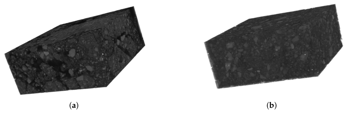
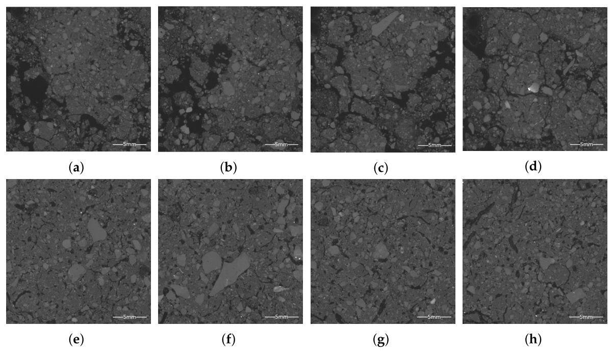
The 3D images of the soil samples used in this study comprised 676 × 676 × 300 voxels. Figure 1 provides a complete 3D visualization of the sample. Three hundred slices were obtained to create 2D CT images 16 bits in depth with a resolution of 676 × 676 pixels. Examples of the original *.TIFF 2D images are shown in Figure 2.

2.2. Segmentation Techniques for CT Images

In digital image processing, segmentation is fundamental for identifying objects of interest. This process involves detecting objects that share similar characteristics, such as grayscale intensity, color, and shape, in the spatial domain. Otherwise expressed, it aims for the pixels constituting an object to be homogeneous and distinct from the pixels of other objects in the image.

Within the family of partitioning clustering algorithms, the core objective is similar to segmentation: to identify natural clusters in the feature space. Patterns that form a cluster share similarities among themselves and differ from patterns in other clusters.

As mentioned, partitioning clustering algorithms are a reliable choice for digital image segmentation. They have been widely used in the detection of pore, solid, and gravel spaces, treetop detection, and other elements in soil CT images [20,21]. In former years, soil CT images were generally of 8-bit depth, which translates to 256 levels of gray intensity. This limitation presented a considerable challenge in identifying solids, gravel, pores, and other elements when characterizing soil samples. Today, most soil CT images have a 16-bit depth (with 65,536 levels of gray intensity), allowing for more precise soil characterization and the use of basic algorithms like k-Means.

The main challenge of this work lies in detecting the cSOCRs in CT images of a soil sample. A primary issue is that pores can be confused with cSOCRs since we operate under the assumption that pixels corresponding to pores have a near-black intensity, while the darker pixels, not belonging to pores, could represent organic carbon. Hence, the task involves defining thresholds to detect pores and subsequently determining another specific threshold in the nonporous region for identifying organic carbon.

To address this challenge, we proposed a dual segmentation strategy. First, we apply the basic algorithm from the partitioning clustering algorithm family, known as k-Means [22], the Fuzzy c-Means [23], and Otsu’s method [24], to distinguish regions corresponding to pores from nonporous regions. These algorithms were selected due to their ability to handle grayscale intensity variations and feature space clustering. FCM and k-Means effectively group similar intensity values, while Otsu’s method provides an adaptive thresholding approach, ensuring accurate initial segmentation in CT images. Then, in the nonporous region, we employ a sub-segmentation method based on the Possibilistic Fuzzy c-Means Clustering Algorithm (PFCM) [25]. This method allows us to identify sub-regions within each segmented class, and within one of the sub-regions of the class closest to the pores, the organic carbon is found.

Although Otsu’s is not classified as a partitioning algorithm, it was proposed for use in the initial segmentation phase. Its distinguishing feature is its ability to determine an optimal threshold by maximizing inter-class variance, a characteristic particularly beneficial for grayscale images. A notable advantage of the Otsu algorithm is its functionality without relying on prior image information, rendering it advantageous for CT image segmentation. Its efficacy has been demonstrated in contexts such as the detection of microcalcifications in mammograms [26] and in the segmentation of soil images [17], where its efficacy has been substantiated.

The following section details the sub-segmentation method and the dual segmentation strategy we used for organic carbon detection.

Sub-Segmentation Method

The sub-segmentation method aims to identify atypical or typical sub-regions within a previously segmented area, object, or group in a digital image [27]. In this process, we first apply the PFCM clustering algorithm [25], which combines the advantages of Fuzzy c-Means [23] and Possibilistic c-Means (PCM) [28], to perform the initial image segmentation. Next, by applying a predefined threshold value to the possibility matrix generated by the PFCM, we distinguish atypical and typical sub-regions within the primary segmented area. This approach highlights areas of interest or abnormalities within a segmented region. The PFCM algorithm provides a promising approach for image sub-segmentation and has potential applications in various fields, including medical diagnosis [29] and soil analysis [17].

Sub-segmentation is a successful technique in digital image processing designed to identify atypical, typical, or unusual sub-regions within the previously segmented areas of a digital image. These sub-regions can be useful for identifying areas of interest during image analysis. However, identifying these atypical sub-regions can be challenging, as they often comprise only a few pixels. In conventional segmentation, detecting these atypical sub-regions may necessitate generating a large number of clusters for image partitioning, rendering sub-segmentation a viable alternative.

Algorithm 1 contains the sub-segmentation process steps.

Algorithm 1 Sub-Segmentation Method

Input: Dataset $\mathbf{Z}$.

$\mathbf{Z}$ represents the image matrix $rxn$, which is flattened into a one-dimensional vector ${\mathbf{v}}_0^T$. Step I. Set parameters $\{a,b,m,c,\eta \}$ for the PFCM algorithm. Step II. Execute the PFCM algorithm to obtain matrices $U=\left[{\mu }_{ik}\right]$, $T=\left[t_{ik}\right]$, and $V=\left[v_{ik}\right]$, respectively representing membership, typicality, and prototypes. Step III. Identify Fuzzy Regions (FR) from matrix U: $S_{i\left(FR\right)}={max}_i\left(\left[{\mu }_{ik}\right]\right),i=1\dots c$. Step IV. Identify Typicality (Possibilistic) Regions (PR) from matrix T: $S_{i\left(PR\right)}={max}_i\left(\left[t_{ik}\right]\right),i=1\dots c$. Step V. Get maximum typicality values: $T_{max}={max}_i\left(\left[t_{ik}\right]\right),i=1\dots c$. Step VI. Select a threshold value $\alpha$, where $0<\alpha <1$. Step VII. Using $\alpha$ and $T_{max}$, separate pixels into two sub-vectors, $T_1$ (typical region) and $T_2$ (atypical region). Step VIII. Generate $T_{2\left(new\right)}$ by mapping atypical pixels using $T_2$ and assign their typicality values to corresponding grayscale pixels. Step IX. Separate $T_{2\left(new\right)}$ pixel into two sub-regions based on prototype $v_i$: if $T_{2\left(new\right)}\ge v_i$ then $S_{i\left(PR\right)}\text{\_}atypRe{g}_{c+i}$, else $S_{i\left(PR\right)}\text{\_}atyRe{g}_{2c+i}$.

Output: $S_{i\left(PR\right)}\text{\_}typica{l}_i$, $S_{i\left(PR\right)}\text{\_}atyRe{g}_{c+i}$ and $S_{i\left(PR\right)}\text{\_}atyRe{g}_{2c+i}.$

Where c is the number of clusters or number of regions, m defines the fuzziness level of the partition, $\eta$ defines the possibilistic level of the partition, whereas a and b weigh the relative importance between the fuzzy and the possibilistic approaches. Even if the parameters m and $\eta$ can take any value in a wide interval, it is classical to use 2 for both parameters. The relative value between a and b offer the option that the results (the prototypes for example) of the PFCM depend more on the fuzzy values or on the typicality values. If a is greater than b, the fuzzy values have a more important weight on the calculus. On the other hand, if b is greater than a, then the typicality values have a more important influence on the results. In order to reduce the noise effects, this last relation must be applied; that is, the value of b must be greater than a [17,20,25].

2.3. A Novel Dual Segmentation Method for cSOCR Detection

Dual segmentation is the novel approach we proposed to detect organic carbon in CT images of soil samples. This process starts by segmenting the original image (without pre-processing) into two classes $\left\{P_1,P_2\right\}$, using the well-known k-Means algorithm, while the Fuzzy c-Means and Otsu’s method can also be used. One of the classes is the pores, and the other is the non-porous region (gravel, solid, and organic carbon spaces). The novelty lies in generating a new vector that contains only the pixels from the non-porous region and their spatial positions in relation to the original CT image.

We then further segment the sample into two regions using the sub-segmentation technique. This provides us with three sub-regions for each region: one typical sub-region and two atypical sub-regions. The atypical sub-region closest to the pores is considered to contain the organic carbon.

A critical aspect of the dual segmentation process is the selection of the threshold value $\alpha$ for the sub-segmentation technique. This choice is crucial because an inappropriate value could exclude cSOCR material or include unwanted material. Since we do not have ground truth images to verify the identification of cSOCRs confidently, we use the value of NU (Non-Uniformity Level) to ensure that the sub-region containing cSOCRs is homogeneous and consistent. The sub-segmentation threshold $\alpha$ was empirically determined as a fixed value that yielded the best results. Although not dynamically adjusted per sample in this study, it can be adaptively optimized to improve case-specific precision.

The necessary steps to carry out this sub-segmentation process are described in detail in Algorithm 2. This technique represents a promising and effective approach for accurately detecting cSOCRs in soil sample images from CT scans.

Algorithm 2 Dual Segmentation Technique for cSOCR Detection

Input: $\mathbf{Z}$, a dataset of 2D soil sample images (16-bit each). $\mathbf{Z}$ represents the image matrix $rxn$, which is flattened into a one-dimensional vector ${\mathbf{v}}^T$.

Step 1: Initialization Set k-Means clustering parameters: $m=2$ and $c=2$. Load the 2D image: ${\mathbf{v}}^T=\mathbf{Z}$. Step 2: Image Segmentation Apply the k-Means clustering algorithm to segment the image, resulting in two clusters: $P_1$ (pores) and $P_2$ (non-porous regions). These clusters are represented in ${\mathbf{v}}_S^T=\left\{P_1,P_2\right\}$, with each element $l_i$, $i=1,\dots ,k$, representing the label associated with the value $v_i$ at position i. Here, $l_i^{P_1}$ and $l_i^{P_2}$ indicate the labels assigned to the elements in $P_1$ and $P_2$ clusters, respectively. Step 3: Nullify Pore Pixels Remove labels in ${\mathbf{v}}_S^T$ corresponding to class pore pixels $P_1$ such that $l_i^{P_1}=Ø$. The updated vector is ${\mathbf{v}}_{SØ}^T$ with null labels and the label for non-porous regions: ${\mathbf{v}}_{SØ}^T=\left\{Ø,P_2\right\}$. Step 4: Generate a New Vector Select only the non-porous class from ${\mathbf{v}}_{SØ}^T$, and replace labels $l_i^{P_2}$ with the pixel intensity value associated in ${\mathbf{v}}^T$. This results in a new vector: ${\mathbf{v}}_{new}^T$. Step 5: Sub-Segmentation Apply sub-segmentation to ${\mathbf{v}}_{new}^T$ with two classes $\left(S_{1\left(PR\right)},S_{2\left(PR\right)}\right)$, resulting in three sub-classes for each class (one typical and two atypical). Step 6: Analyze Sub-Classes Organic carbon is typically present in one of the sub-classes: $S_{i\left(PR\right)}\text{\_}atypicalRegio{n}_{\{c+i,left\}}$. Step 7: Label Update Update labels in ${\mathbf{v}}_{SØ}^T=\left\{Ø,P_2\right\}$ using labels from ${\mathbf{v}}_{sub}^T$ instead of $P_2$. The resulting vector is ${\mathbf{v}}_{dualseg}^T=\left\{Ø,{\mathbf{v}}_{sub}^T\right\}$. Step 8: Construct Sub-Segmented Image Apply unflattening to ${\mathbf{v}}_{dualseg}^T$ to obtain the dual-segmented image.

Output: Dual-segmented image for carbon detection.

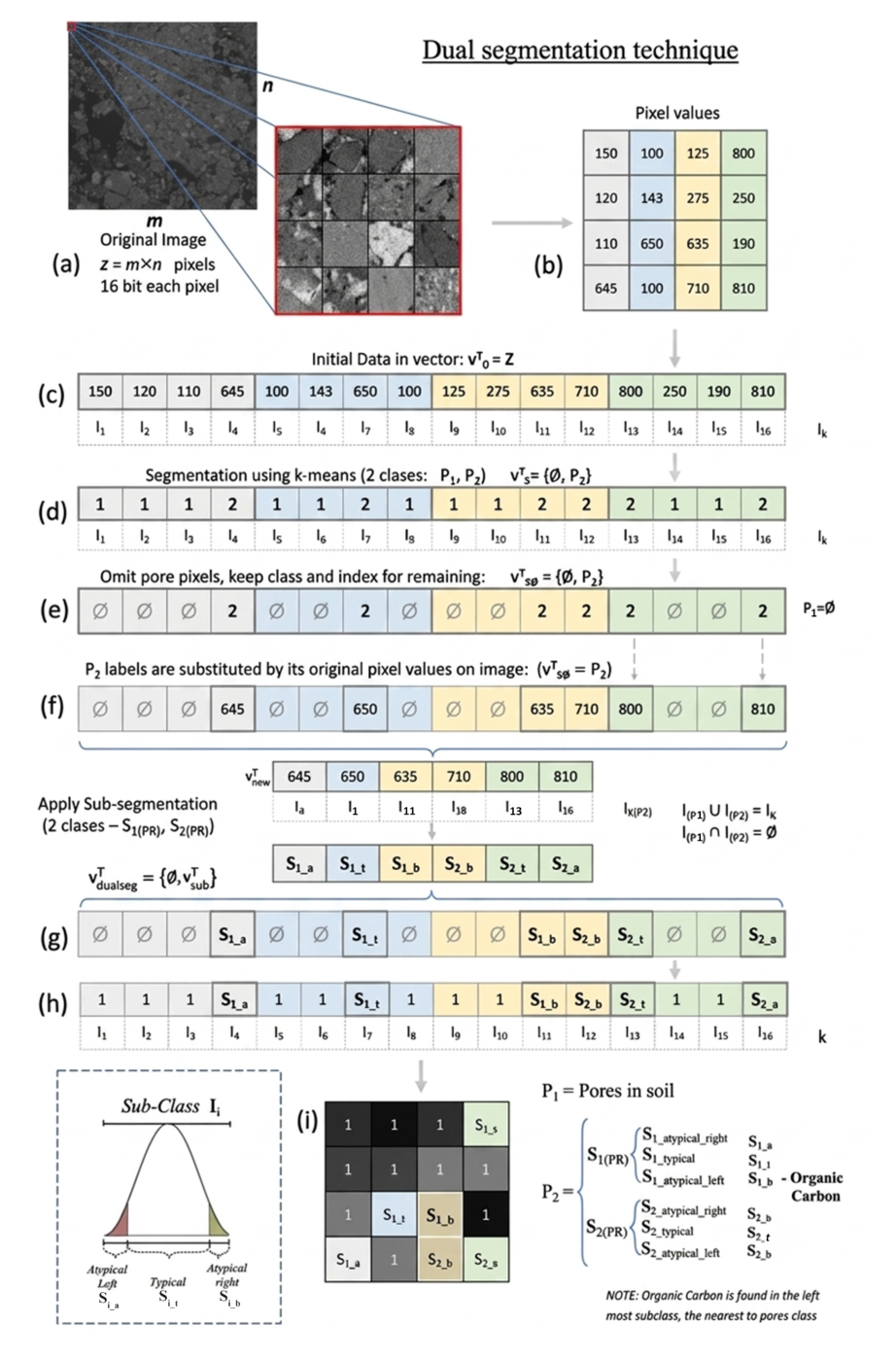
Figure 3 illustrates our dual segmentation approach for detecting cSOCRs in soil CT images. The following are the key steps for understanding this proposal:

Dual Segmentation to detect cSOCRs in CT soil images:

(a)

Displaying a slice of the entire set of 2D images from the soil sample.

(b)

Represent the pixel intensity values in a 16-bit matrix.

(c)

Matrix flattened into a vector.

(d)

Segmenting the image to detect macropores/pores and the rest, using a standard clustering algorithm, generating a vector with labels in two regions: pores and non-pores.

(e)

Marking the pore labels as null.

(f)

Replacing the intensity values of the non-porous region to create a new vector intended for the sub-segmentation technique.

(g)

Obtaining labels for the sub-regions, for both atypical and typical samples in each region, and adding null labels on the spatial location of each pixel in the image.

(h)

Combining the pore labels with those of the sub-segmentation and reconstruction of the image through unflattening.

2.4. Evaluation Criterion

The non-uniformity measure serves to assess the quality of segmentation, in cases where ground truth information is not available [30,31]. This criterion or metric is computed as follows:

$$NU={\displaystyle \frac{B}{T}}·{\displaystyle \frac{{\sigma }_P^2}{{\sigma }^2}},$$

(1)

where B represents the number of pixels in the region of interest (pore, carbon, etc.), T is the total number of pixels in the segmented image ($r\times n$), and respectively, ${\sigma }_P^2$ and ${\sigma }^2$ are the variance of the grayscale values within the region of interest and in the entire image. A NU value close to 0 indicates that the segmented region is highly homogeneous, while values greater than or close to 1 indicate lower homogeneity in the segmented region. This measure serves as a criterion for assessing segmentation quality regarding homogeneity, as it quantifies the degree of similarity among pixels within the identified region.

These steps achieve dual segmentation that facilitates the detection of organic carbon in soil CT images.

3. Computational Results and Analysis

Dual segmentation was applied to two different soil samples. Subsequently, a 3D image of cSOCRs and pore distribution was generated with the results being used to characterize the soil samples. The selected parameters for the PFCM algorithm were $a=1$, $b=4$, $c=2$, $m=2$, and $\eta =2$.

3.1. Novel Dual Segmentation

As mentioned, the dual segmentation process comprises two stages:

3.1.1. Initial Segmentation of CT Images and Evaluation

In the first stage, the 300 CT images from soil samples I and II were individually segmented. Sample I was segmented into two regions, and sample II was segmented into three. The two regions that do not belong to the pore category were merged into one to obtain the non-porous region. This process obtained two regions for each CT image $\left\{P_1,P_2\right\}$ for the detection of macropores/pores and non-pores (cSOCRs, gravel, and solid space). In addition, the NU values were computed for each 2D image slice to evaluate quantitatively the homogeneity of macropores and pores, given the absence of ground truth reference images. A NU value close to zero indicates a high degree of uniformity within the segmented region, confirming the consistency of the segmentation process. Conversely, higher NU values suggest increased variability in grayscale intensity, potentially indicating segmentation inconsistencies.

(a)

Detection of macropores/pores using standard clustering algorithms

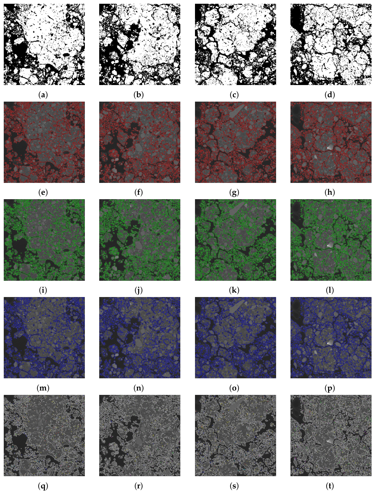
Figure 4 shows the segmentation results of CT images (Im_001, Im_070, Im_180 and Im_280) for Soil Sample I. The first row (Figure 4a–d) shows binary images generated by the k-Means algorithm. In these images, black represents macropores, while white corresponds to the non-porous region, including spaces for cSOCRs, gravel, and solids. This non-porous region was used in Stage II for cSOCR detection.

The edges generated by each algorithm are highlighted in the subsequent rows. The second row (Figure 4e–h) shows the edges highlighted in red by the k-Means algorithm. The third row (Figure 4i–l) shows the green edges generated by the FCM algorithm. Finally, the fourth row (Figure 4m–p) shows the blue edges obtained by the Otsu method.

In Figure 4q–t, the last row represents the results of combining the algorithms. The white edges indicate areas where the algorithms coincide, while small pores are detected by one algorithm but not the others. However, we lacked a ground truth image to determine which method outperformed the others. From the NU values provided by the algorithms, we concluded that any of the three segmentation algorithms are a good choice for macropore detection. As mentioned, we chose the k-Means algorithm because it is easy to apply.

(b)

Results of NU and percentage of Macropores (Soil Sample I) and pores (Soil Sample II)

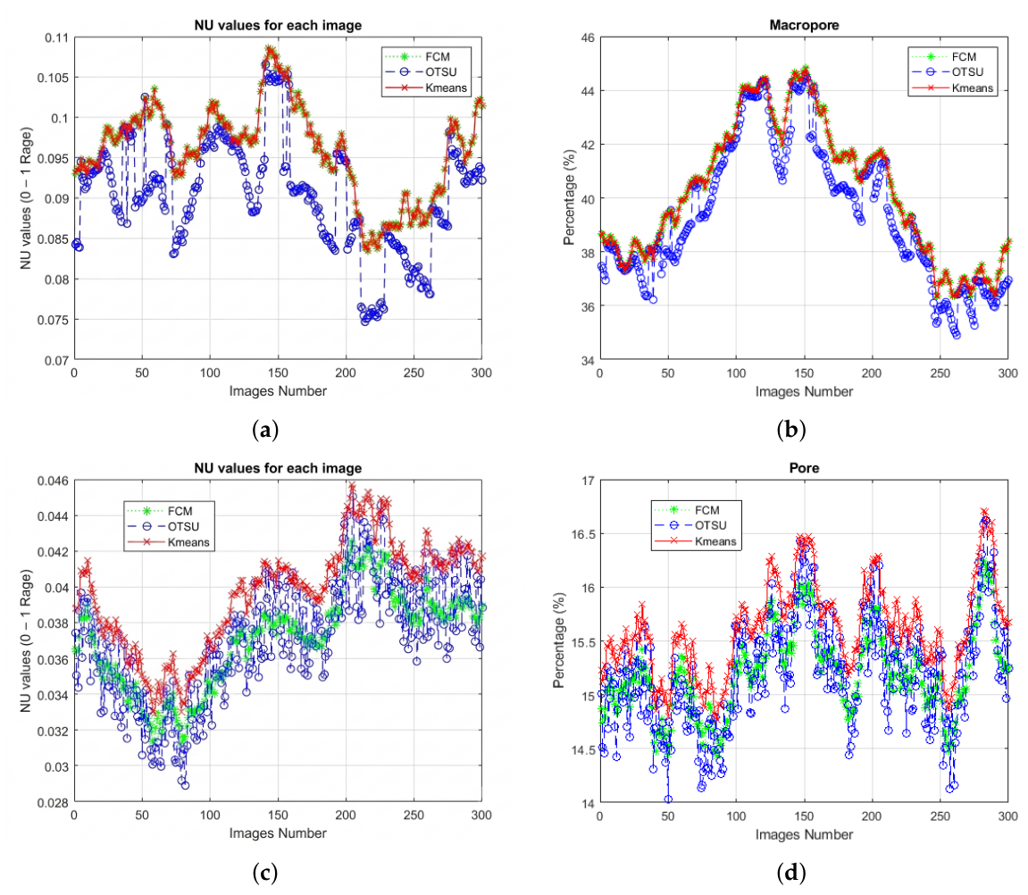
Figure 5 presents the NU values and the percentages of macropores and pores of the 300 images of soil samples I and II. These data were obtained through the initial segmentation of the CT images in Stage I of our study.

Figure 5a,c display the NU values for the segmented region of macropores and pores using the three aforementioned algorithms. The NU values for the Soil Sample I (see Figure 5a) range from 0.11 to 0.07; this is attributed to the significant contrast between the macropore region and the non-macropore region. The results of the k-Means algorithm indicate consistent homogeneity in the structure of macropores across all images. This underscores the robustness of the k-Means analysis, which relies on a strict pixel assignment, enabling effective segmentation, particularly in 16-bit images. The percentages of macropores (see Figure 5b) vary in the range of 35 to 45 percent with almost half of the space in the sample being macropores. The percentage transition is gradual and reaches its peak in the central sections of the soil sample.

For soil sample II, see Figure 5c, the NU values range between 0.046 and 0.03, very close to zero. Similarly to the previous sample, this is due to the high contrast between the porous and non-porous regions. The results of the k-Means algorithm indicate consistency in the structure of the pores in all images of the soil sample. The percentages of pores (see Figure 5d) vary between 14.5 and 16 percent, with almost a quarter of the soil sample space corresponding to pores.

The NU values for FCM in soil sample I (see Figure 5a) are similar to those of k-Means, in some cases practically identical. Despite the fuzzy nature of the FCM algorithm, where a pixel has some membership in both regions, the high contrast makes the differences in segmentation imperceptible. Therefore, the percentages of macropores were very similar to those obtained by k-Means (see Figure 5b).

For Soil Sample II (see Figure 5c), the NU values for FCM were almost parallel to but below those of k-Means. However, similar to sample I, the result was practically identical to that of k-Means.

The NU values in Soil Sample I (see Figure 5a) for the Otsu algorithm were slightly lower than those of k-Means and FCM, due to its focus on finding the optimal threshold that maximizes the variance between the two classes. This led to slightly lower percentages of macropores, which in some images coincided with those obtained by FCM and k-Means.

Finally, the NU values for the Soil Sample II (see Figure 5c) in some images were below those of k-Means and FCM, and in other images, they coincided with the results of FCM and k-Means.

In summary, all three algorithms demonstrated a remarkable ability to detect macropores and pores for Soil Samples I and II, owing to the high contrast between pores/macropores and non-pores/macropores, as well as the 16-bit depth of the CT images. Any of these algorithms is suitable for the first stage of dual segmentation. The only difference lies in that for sample I (macropores), we segmented the CT images into two regions, while for sample II (pores), it was three regions. Therefore, we have chosen the k-Means algorithm because of its widespread familiarity and ease of use.

3.1.2. Sub-Segmentation and cSOCR Detection

In Stage II, we focused exclusively on the non-porous region of each CT image (cSOCRs, gravel, and solid spaces) from soil samples I and II, along with their spatial information. We applied segmentation to this region in two parts: $S_1$ (gravel and cSOCRs) and $S_2$ (solids), using the PFCM algorithm. The segmentation was performed with the partition of the possibility matrix T and obtained two possibilistic regions: $S_{1\left(PR\right)}$ y $S_{2\left(PR\right)}$.

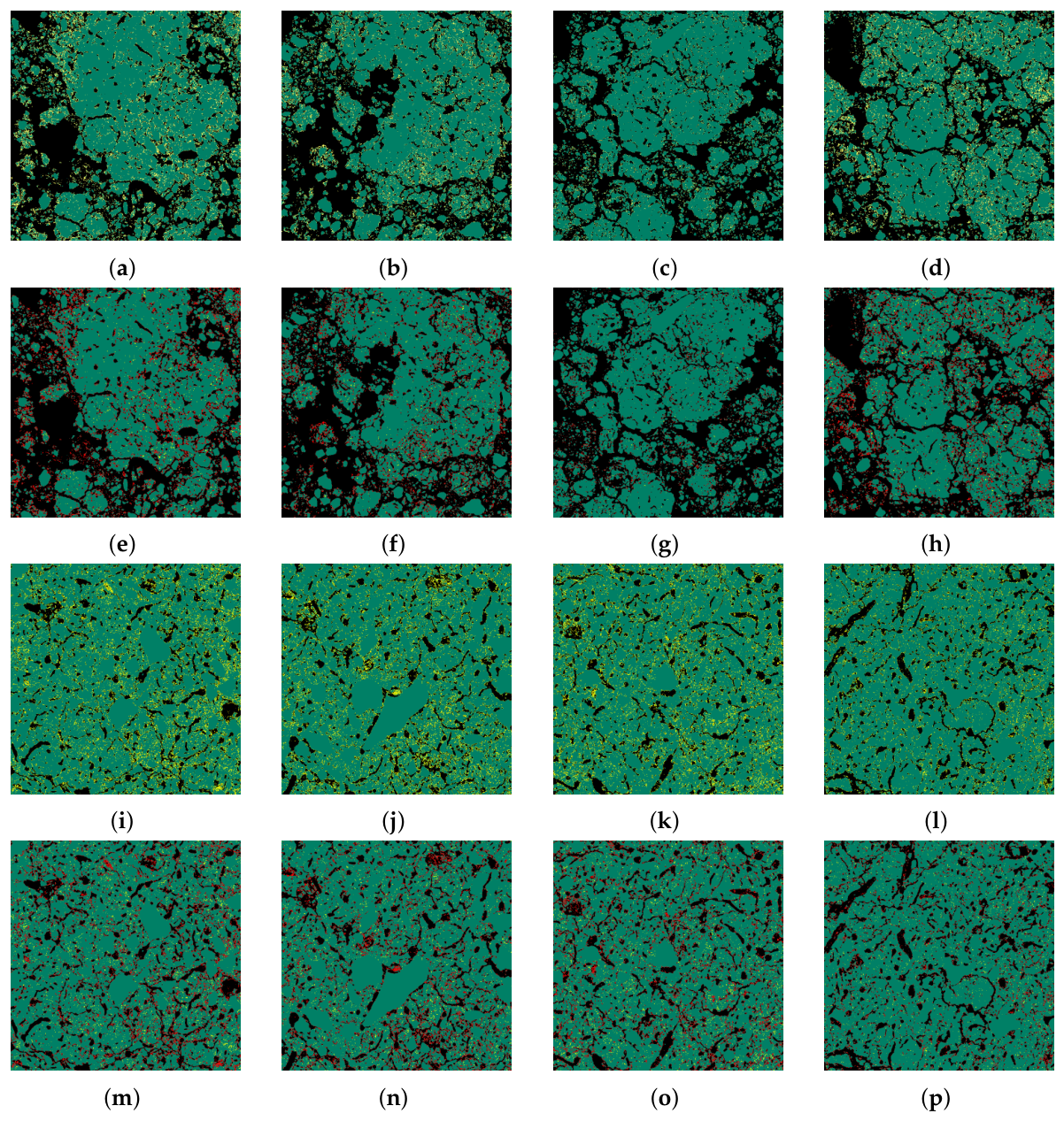
The results for Soil Sample I are shown in Figure 6a–d, while the results for Soil Sample II are presented in Figure 7a–d. For both Figures, the regions $S_{1\left(PR\right)}$ (gravel, including cSOCRs) are shown in yellow and $S_{2\left(PR\right)}$ (solids) in blue. Black represents the region $P_1$ found by the k-Means algorithm in the first stage. cSOCRs are located in a sub-region of the gravel space (see

Table 1. Representation of Typical and Atypical Sub-Regions Using Color Coding.

Material	Type	Color	Sub_Region
Gravel $S_1$(PR)	$S_1\text{\_}atyReg\text{\_}right$	Orange	5
	$S_1\text{\_}typical$	Yellow	1
	$S_1\text{\_}atyReg\text{\_}left$	Red	3
Solid Space $S_2$(PR)	$S_2\text{\_}atyReg\text{\_}right$	Cyan	6
	$S_2\text{\_}typical$	Blue	2
	$S_2\text{\_}atyReg\text{\_}left$	Sky-blue	4

).

Subsequently, we applied the Sub-segmentation method to the 300 CT images using a threshold value of $\alpha =0.2$ for Soil Samples I and II. This resulted in the emergence of three distinct sub-regions within the gravel $S_{1\left(PR\right)}$ and the solid spaces $S_{2\left(PR\right)}$. Each space includes one typical and two atypical sub-regions. In particular, the atypical sub-regions adjacent to the carbon within the gravel space contain cSOCRs. In Figure 6a–d, the macropores, presented in black, occupy almost half of the space, while the gravel in yellow and solids in blue occupy the least space.

In the second row, Figure 6e–h, the results of the sub-segmentation for detecting cSOCRs are shown. The solids region $S_{2\left(PR\right)}$ was partitioned into three sub-regions: blue represents the typical sub-region $S_{2\left(PR\right)}\text{\_}typica{l}_2$, while the sky blue areas ($S_{2\left(PR\right)}\text{\_}atyRe{g}_{4,left}$) and cyan represent the ($S_{2\left(PR\right)}\text{\_}atyRe{g}_{6,right}$) atypical sub-regions. The cyan sub-region corresponds to pixels with higher grayscale intensity in the solids space near white in the CT images, while the sky blue represents pixels with lower intensity in that space.

The gravel space $S_{1\left(PR\right)}$ was also partitioned into three sub-regions: yellow represents the atypical region $S_{1\left(PR\right)}\text{\_}typica{l}_1$, which is the dominant area, while red ($S_{1\left(PR\right)}\text{\_}atyRe{g}_{3,left}$) and orange ($S_{1\left(PR\right)}\text{\_}atyRe{g}_{5,right}$) represent the respective atypical regions. The orange sub-region corresponds to pixels with higher grayscale intensity in the gravel space, i.e., close to the solid space, while the red sub-region represents pixels with lower grayscale intensity, and they are the closest to the macropore region. This red sub-region is of interest and represents the cSOCRs in Soil Sample I.

The last row in Figure 6i–l presents binary images to highlight cSOCRs. The white emphasizes the presence of cSOCRs in Soil Sample I. These images represent the successful detection of cSOCRs in Soil Sample I, which is particularly relevant for applications in, e.g., soil characterization and soil quality assessment. The accurate detection of cSOCRs is essential for understanding soil’s properties and managing its health, making this stage a critical step within the dual segmentation process.

Figure 7 shows the dual segmentation for the detection of cSOCRs in Soil Sample II (which includes pores). In Figure 7a–d, the pores, represented in black, constitute approximately one-fourth of the space of Soil Sample II, while the gravel in yellow is conspicuously the predominant part, and the solids are presented in blue.

The second row, Figure 7e–h, presents the results of the sub-segmentation to detect cSOCRs. For this image set partition, the color assignment is the same as in Figure 6e–h, recalling that the atypical sub-region is assigned red coloring.

In the last row of Figure 7i–l, binary images are presented to highlight the cSOCR space in Sample II. Similar to the previous figure, white is used to emphasize the cSOCRs. In these images, a higher percentage of cSOCRs is observed compared to sample I. This difference could be attributed to the higher presence of gravel in Sample II, resulting in a higher number of cSOCRs. The direct relationship between the presence of gravel and the content of cSOCRs highlights the importance of understanding the soil composition to interpret the results of dual segmentation accurately.

To understand the impact of carbon in a soil sample, it is crucial to distinguish between cSOCRs near or surrounding soil macropores/pores and cSOCRs separated from these macropores/pores, as both have significant effects on various soil properties and aspects. cSOCRs located in proximity to soil macropores/pores act as a gradually available nutrient source for plants, enhance soil water retention capacity, strengthen soil stability by functioning as a binding agent, stimulate beneficial microbial activity, and ultimately contribute to higher soil quality. In contrast, cSOCRs separated from macropores/pores may result in reduced nutrient availability, lower water retention, decreased soil stability, limited microbial activity, and compromised soil quality. This distinction is essential to understand how the interaction and location of cSOCRs in the soil impact its functionality and its ability to support vegetation and agricultural activities.

3.2. cSOCR Distribution Around Macro/Pores

In this section, the distribution of cSOCRs revealed through dual segmentation in Samples I and II is analyzed. Figure 8 makes a distinction between cSOCRs near macropores/pores and cSOCRs found away from them.

In the first row (Figure 8a–d), macropores are highlighted in black, cSOCR spaces in yellow, and gravel, along with solid spaces, in green. These visualizations show that cSOCRs are predominantly concentrated near the macropores. The third row of Figure 8i–l shows the distribution of cSOCRs in Sample II, also highlighting the proximity to the pores.

Moving to the second row of images (Figure 8e–h), the cSOCRs around the macropores is highlighted in red, while the distant cSOCRs is yellow. Consequently, the bulk of the cSOCRs is revealed to cluster around the macropores. Figure 8m,n, presents more details on the cSOCRs around the pores in Sample II, highlighting that a significant amount of cSOCRs is consistently found near the pores.

This analysis of cSOCR distribution enhances our understanding of the intricate dynamics of the soil and lays the groundwork for unraveling the nuanced interaction between macropores and cSOCRs.

NU Results and cSOCRs Percentage Around and Away from Macro/Pores

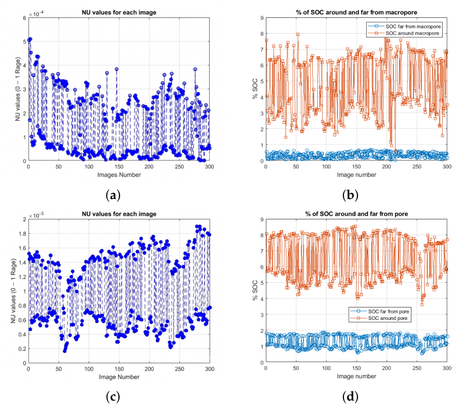
Figure 9 presents the NU values for the cSOCRs obtained through dual segmentation, along with the percentages of cSOCRs in each of the images of soil samples. Figure 9a evidences notable homogeneity in the analyzed regions, confirming that cSOCRs were detected effectively. The maximum NU value for one of the images was 0.0005096, while the minimum value was 2.23 × ${10}^{-7}$. This narrow variation indicates a consistent structural uniformity in the macropores across the images, highlighting the robustness of the analysis.

Therefore, for sample II, the maximum NU value was also very close to zero, indicating highly homogeneous and well-identified cSOCR regions according to the NU values.

The percentage of cSOCRs around and away from the macropores for sample I is presented in Figure 9b, where a notable fluctuation between images was observed, ranging between approximately 3 and 7 percent. These considerable variations can be attributed to two main factors: slight gradations in gray intensity between the CT images of each scan slice and using a fixed threshold in the sub-segmentation method, along with image partitioning through the possibility matrix. In contrast, the percentage of cSOCRs not connected to the macropores was <1 percent.

In the case of Sample II (see Figure 9c), the percentage of cSOCRs in the vicinity fluctuated between 5 and 8 percent, while for cSOCRs away from the pores, it varied between 1 and 2 percent.

The results obtained through dual segmentation reveal a remarkable homogeneity in the regions analyzed, indicating an effective detection of cSOCRs. The narrow variation in NU values, with a maximum approaching zero, emphasizes the consistent uniformity of the macropore structures across the images, validating the robustness of the analysis. These results provide a detailed understanding of the distribution of cSOCRs relative to macropores, allowing a deeper understanding of heterogeneity and connectivity in the soil studied.

This approach enables the precise detection of macropores and the identification of candidate organic carbon regions in soil sample images, providing valuable information for their characterization and study. The dual segmentation process is essential for detecting candidate organic carbon regions in soil sample images and constitutes a crucial step in their characterization. Below, we provide specific details of one stage in the dual segmentation process.

3.3. 3D Reconstruction of cSOCRs, Macropores, and Pores in Soil Samples

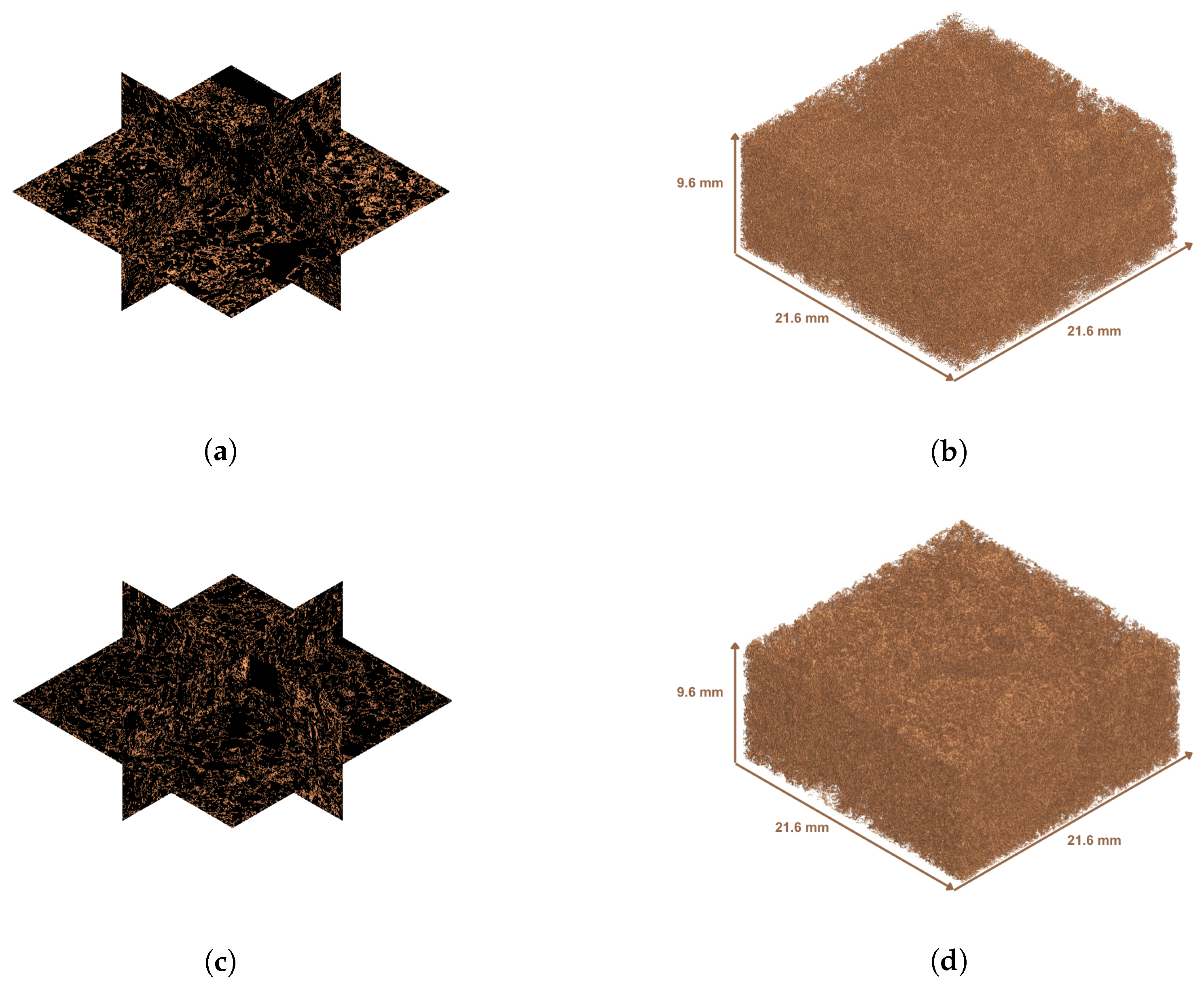
The fundamental reason for performing three-dimensional (3D) reconstruction is to visualize comprehensively the size, shape, and distribution of both cSOCRs and macropores/pores. This volumetric representation affords the ability to assess qualitatively the potential dynamics of these components in the soil. This section presents the 3D reconstruction of macropores (in sample I) and their respective cSOCRs (both close and peripheral), as well as the pore (in sample II) and its corresponding cSOCRs (both nearby and more distant). Dual segmentation enabled the three-dimensional reconstruction of any of the aforementioned components. This approach offered a detailed and comprehensive view of the structure and spatial arrangement of macropores, pores, and cSOCRs, allowing us to explore and understand their interrelationships more deeply.

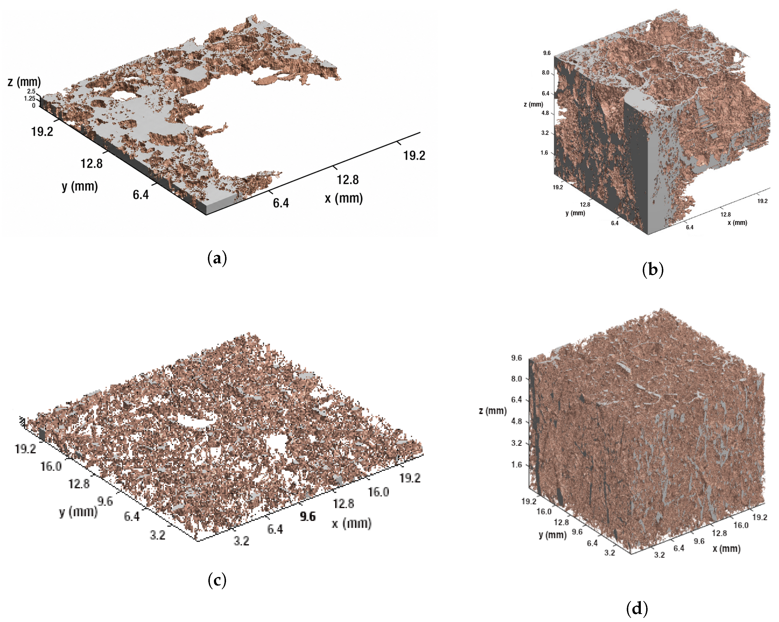
Figure 10a presents the results of the first stage of dual segmentation to identify macropores in Soil Sample I. Fifteen consecutive images ($Im\text{\_}001$–$Im\text{\_}015$) were superimposed to analyze the connectivity in the macropores’ space and assess their size, shape, and continuity. Figure 10a demonstrates a clear alignment of objects across the images, validating the results.

Figure 10b displays the results of the first stage of dual segmentation to identify pores in Soil Sample II. Fifteen consecutive images ($Im\text{\_}001$–$Im\text{\_}015$) were superimposed to analyze the pores’ space and assess their size, shape, and continuity. Figure 10b demonstrates a clear alignment of objects across the images, validating the results.

The superposition of the 300 images ($Im\text{\_}001$–$Im\text{\_}300$) in Figure 10b,d provided a detailed perspective of the three-dimensional structure of macropores in both samples, allowing a comprehensive assessment of their distribution and geometric characteristics.

3D Reconstruction of cSOCRs via Dual Segmentation

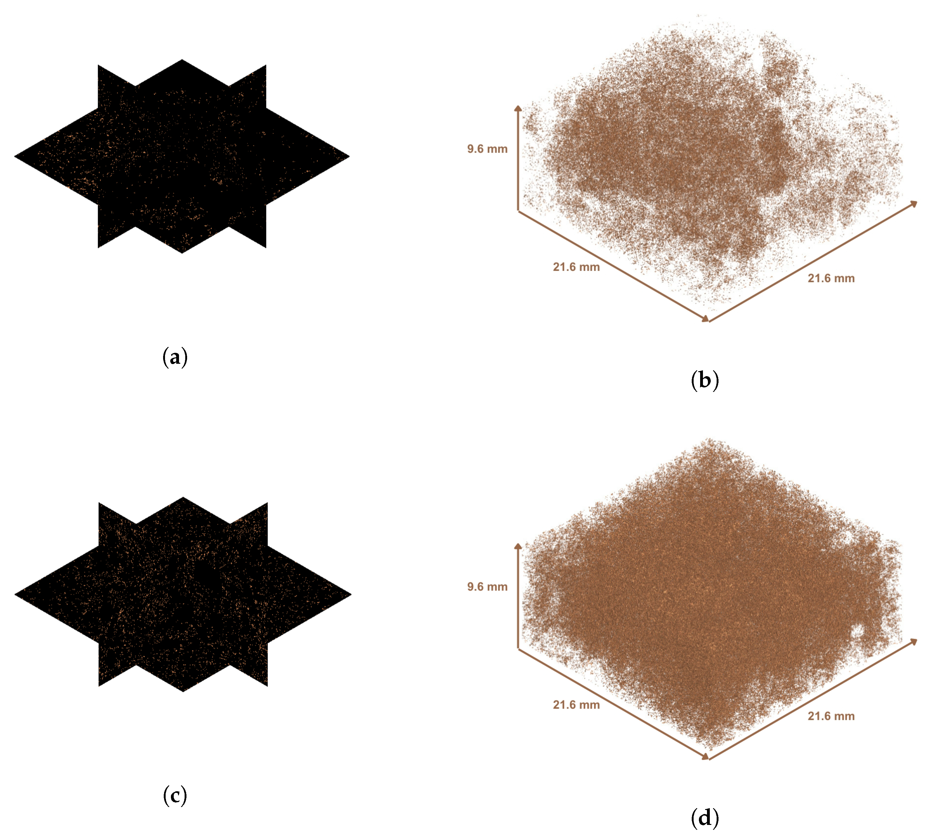
The 3D reconstruction of cSOCRs through dual segmentation provided a detailed view of its spatial distribution. In this section, we examined the reconstruction of cSOCRs both around macropores/pores and in distant areas. This approach allowed analysis of the local structure near the soil features and the variation in the cSOCR distribution in Soil Samples I and II.

Figure 11 and Figure 12 exhibited 3D orthoslices that provide a detailed internal view of the 3D reconstructions of cSOCRs in Samples I and II. This facilitated a more precise qualitative assessment. In addition, the 3D reconstruction of cSOCRs detected through dual segmentation in both soil samples is presented. These expanded visual representations provide a deeper understanding of the distribution and three-dimensional structure of cSOCRs both in the immediate vicinity of macropores/pores and in more distant areas.

(a)

For the cSOCRs around the macropores/pores:

In Figure 11a,c present 3D orthoslices representing the cSOCRs adjacent to the macropore and the pore in Samples I and II. Figure 11b,d show 3D reconstructions of the cSOCRs in proximity to the macropore/pore, allowing a qualitative review of its distribution and density.

(b)

For the cSOCRs away from the macropores/pores:

In Figure 12a,c present 3D orthoslices that represent cSOCRs distant from the macropore and pore in Samples I and II. Figure 12b,d show the 3D reconstructions of the cSOCRs relative to the macropore/pore, allowing a qualitative review of its distribution and density.

3.4. Soil Samples Characterization via Dual Segmentation

Among other aspects, characterizing soil is essential for understanding its quality, water retention capacity, and its role in the carbon cycle. Soil’s components such as gravel, pores, cSOCRs, and solids influence its functionality and are important in agriculture, ecology, resource management, and related fields. In this context, soils play a crucial role in the environment, with cSOCR sequestration being a key component. cSOCRs improve soil quality and fertility and contribute to moisture and nutrient retention, reducing erosion. The loss of organic matter in the soil affects agricultural and forestry productivity, as well as food security. Increasing cSOCRs preserves soil fertility and improves productivity and mitigates the release of atmospheric carbon dioxide (${\mathrm{CO}}_2$), balancing food security and climate change concerns. Effective understanding and management of cSOCRs are fundamental steps for successful soil conservation strategies.

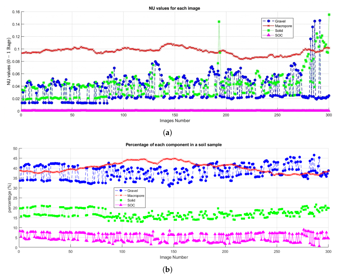
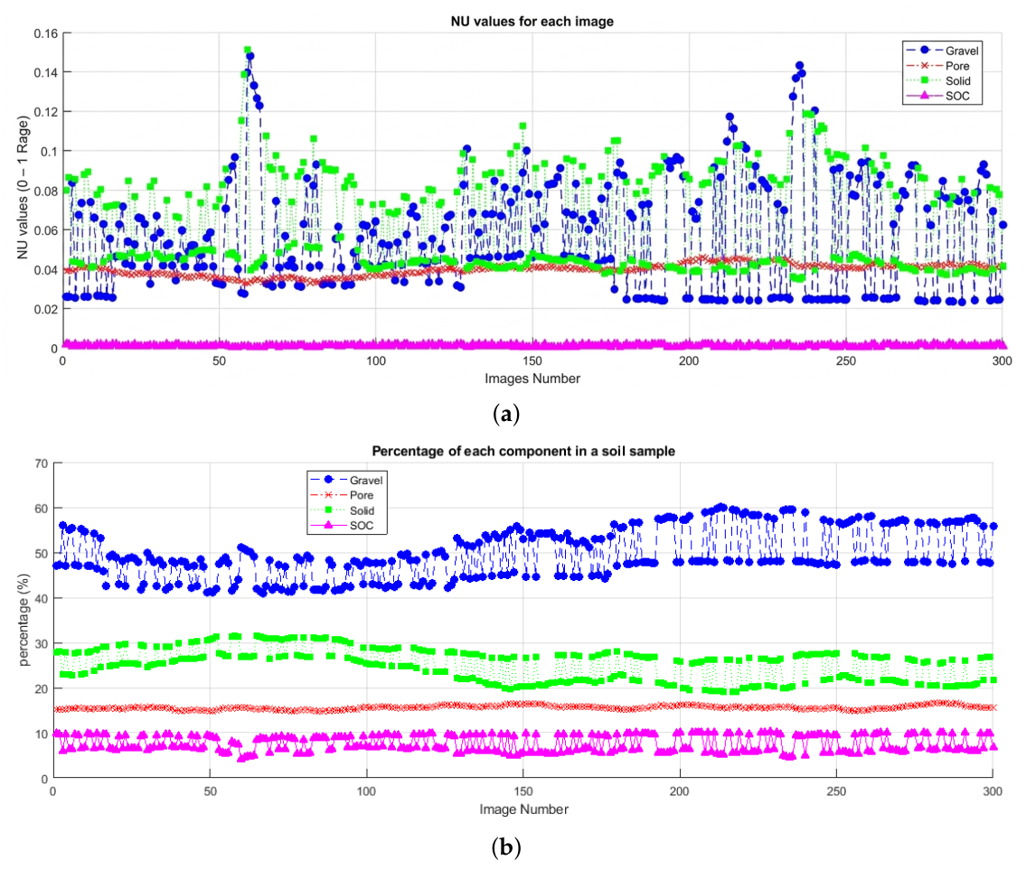
The dual segmentation of 300 CT images of soil samples I and II determined the percentages and NU values per each image of (a) macropores/pores, (b) solids, (c) gravel, and (d) cSOCRs. Such analysis facilitates a detailed understanding of the composition and structure of the soil, allowing its properties to be characterized precisely.

3.4.1. Characterization of Sample I

In Figure 13a, the NU values are presented for each component of Soil Sample I. The NU values for macropores ranged from 0.08 to 0.11, while for gravel and solids, they were notably similar, ranging between 0.01 and 0.08. In the case of cSOCRs, the values closely approached zero. These results indicate that the detected spaces exhibit high homogeneity in the soil samples’ CT images.

Hence, we can conclude that the spaces detected in each of the soil images were highly homogeneous.

Figure 13b presents the percentages of each component in Soil Sample I. For macropores, the percentage ranged from approximately 36% to 45%; for gravel, it varied between 30% and 45%; for solids, it ranged from 14% to 20%; and finally, for cSOCRs, it oscillated between 2% and 9%.

3.4.2. Characterization of Sample II

In Figure 14a, the NU values are presented for each component of Soil Sample II. The NU values for the pores were 0.04, while for gravel and solids, they were very similar and ranged between 0.02 and 0.12. In the case of cSOCRs, the values were very close to zero. These results indicated that the detected spaces exhibited high homogeneity in the CT images of the soil sample.

We can say that the spaces detected in each of the CT images of Soil Sample II were highly homogeneous.

Figure 14b presents the percentages of each component in Soil Sample II. For the pores, the percentage remained constant at approximately 15%; for gravel, it oscillated between 40% and 60%; for solids, between 18% and 32%; and finally, for cSOCRs, it fluctuated between 5% and 10%.

These results provided a detailed insight into the composition of the soil samples, highlighting the relative distribution of their components. The homogeneity of the detected spaces suggested a uniform structure in Soil Samples I and II, which is crucial to understanding their physical properties and the potential impact on processes such as water retention and the carbon cycle.

4. Discussion

Dual segmentation is a novel approach for characterizing soil samples, providing a detailed representation of key components such as pores, cSOCRs, gravel, and solids. However, one of its main challenges is its high computational cost, as segmentation must be performed on each individual CT slice, increasing processing time and resource demand. The selection of the sub-segmentation threshold is another critical factor. In this study, it was empirically determined and applied uniformly to the entire soil sample. A more adaptive approach, where the threshold is dynamically adjusted for each image, could improve segmentation accuracy and adaptability across varying soil conditions. Despite these challenges, the proposed method provides a detailed visualization of cSOCR distribution, which is essential for optimizing agricultural practices. Identifying cSOCR-rich areas allows for targeted tillage, minimizing soil disturbance and enhancing conservation efforts. This approach also contributes to reducing ${\mathrm{CO}}_2$ emissions, supporting climate change mitigation. Hyperspectral imaging has been explored as an alternative for cSOCR detection, but it is limited to surface analysis [32,33]. In contrast, CT imaging provides structural information, allowing for a deeper understanding of cSOCR distribution. Dual segmentation facilitates cSOCR detection and identifies pores, whose characteristics can be used to train neural networks for automatic detection applications [34]. However, the method is sensitive to variations in soil texture and composition, particularly in the presence of minerals with densities similar to cSOCRs. Although cSOCRs typically appear as dark areas in CT images due to their lower density, other components such as air- or water-filled pores and low-density minerals may generate similar signals, affecting segmentation accuracy. CT imaging enables a detailed analysis of soil microstructure, including pore networks and cSOCR distribution across different layers. This structural insight is crucial for understanding the role of pore connectivity in cSOCR stabilization and decomposition, as highlighted by Kravchenko et al. [34,35]. For precision agriculture, multiple high-quality CT scans are required to achieve accurate cSOCR mapping. Identifying regions requiring compost application or soil improvement through precise cSOCR quantification enhances land management efficiency. Future research should focus on developing cost-effective and scalable methodologies for cSOCR detection, ensuring broader adoption in sustainable agriculture. By integrating CT imaging with dual segmentation, our study enhances the ability to quantify and visualize cSOCR distribution in undisturbed soil samples, providing a complementary approach to previous research focused on pore connectivity and carbon protection mechanisms. These findings highlight the necessity of refining pore-scale models for predicting soil carbon dynamics and improving strategies for carbon sequestration and sustainable soil management.

5. Conclusions

The results of this study confirm that the k-Means, FCM, and Otsu methods are highly effective, in identifying macropores/pores during the first stage of dual segmentation. Most of the NU values were below 0.1 for Soil Samples I and II, indicating remarkable homogeneity in each of the 300 2D images. This homogeneity translates into a robust connectivity of macropores/pores across the 2D images, clearly reflected in the three-dimensional reconstruction of the soil sample from the complete set of 2D binary images representing macropores/pores.

In the second stage of dual segmentation, we effectively identified gravel and solid spaces in both samples, particularly noting the successful detection of cSOCRs in an atypical region of the gravel space, with NU values closely approaching zero, ensuring accurate detection.

This study demonstrates that dual segmentation using 16-bit CT images is a robust option for characterizing soil samples and assessing soil quality. However, further research should be undertaken on applying the dual segmentation to different soil types. Additionally, exploring a non-constant threshold and a voxel-based segmentation could potentially improve on our method.