Quantum Computing and Adaptive Mechanism-Based Bounty Hunter Optimizer for Numerical Optimization and Bankruptcy Prediction

Abstract
1. Introduction
- (1)
- A quantum-computing-enhanced initialization strategy is introduced. Through qubit encoding and a quantum rotation mechanism, the distribution diversity of the initial population is improved, allowing candidate solutions to cover the search space more sufficiently. This helps reduce the sensitivity of the original BHO to the quality of the initial population and provides a higher-quality starting point for subsequent global search.
- (2)
- An adaptive Levy flight strategy is designed. To address the problems that the original BHO may suffer from in complex multimodal problems, such as rapid shrinkage of the search range and insufficient ability to escape from local optima, Levy flight perturbation is introduced. An adaptive mechanism dynamically adjusts the perturbation intensity so that the algorithm maintains strong global exploration capability in the early stages of iteration and gradually improves local search stability in the later stage. This further improves the optimization efficiency of the algorithm in complex search spaces.
- (3)
- An adaptive differential operator is constructed. To further improve the later-stage exploitation and fine-grained search ability of the algorithm, the idea of differential evolution is introduced in the later stage of iteration. New candidate solutions are generated by using difference information among individuals, and the differential perturbation intensity is adaptively adjusted according to the search process. This strategy helps enhance information interaction among individuals, alleviates the insufficient convergence accuracy of the algorithm in the later stage, and improves the stability of solutions.
- (4)
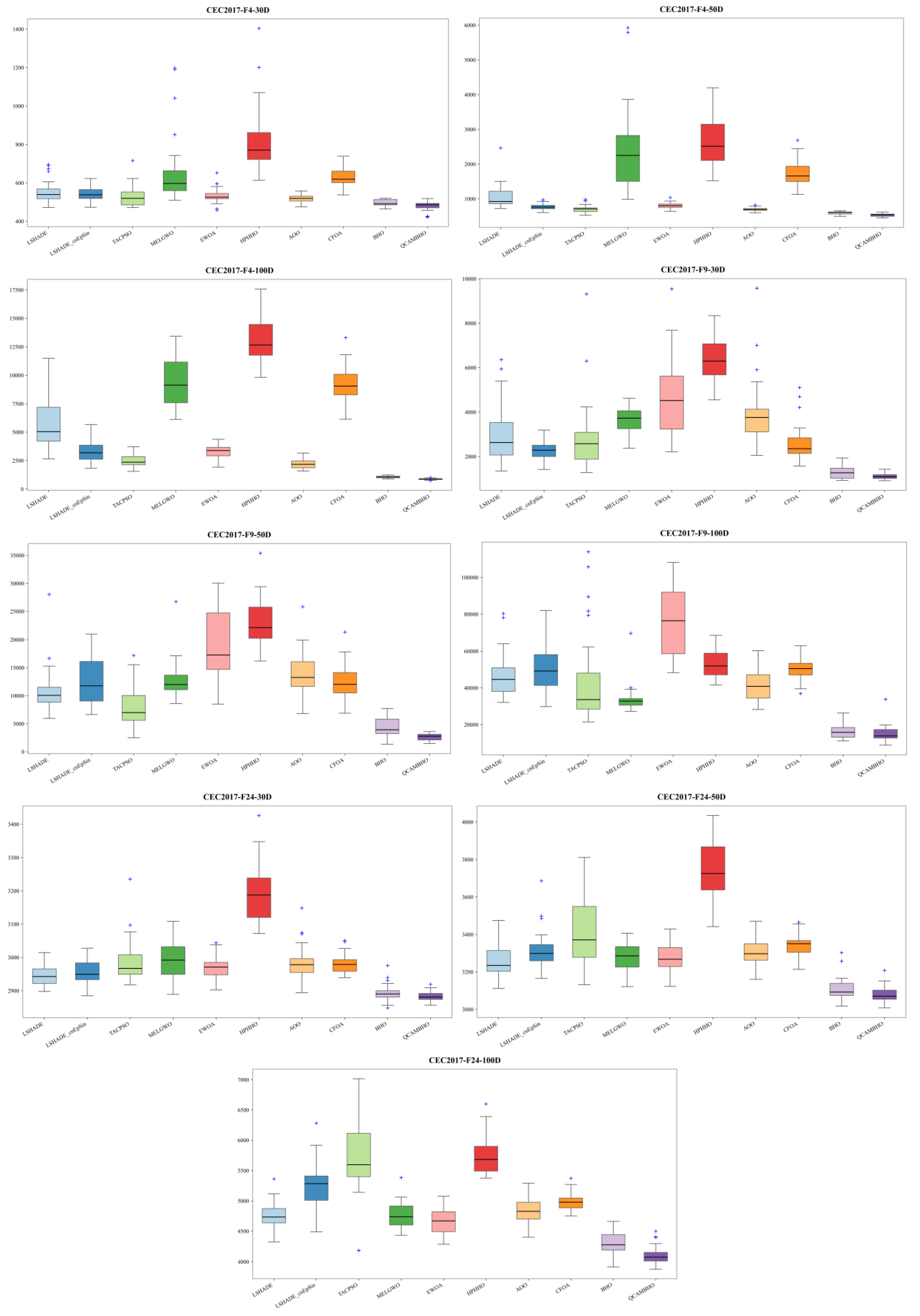
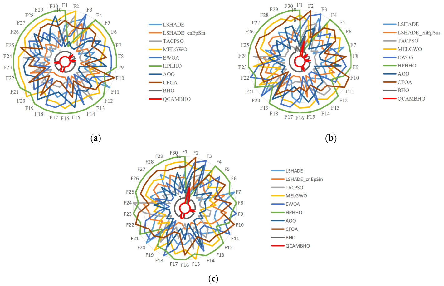
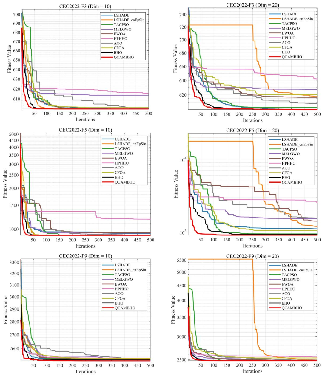
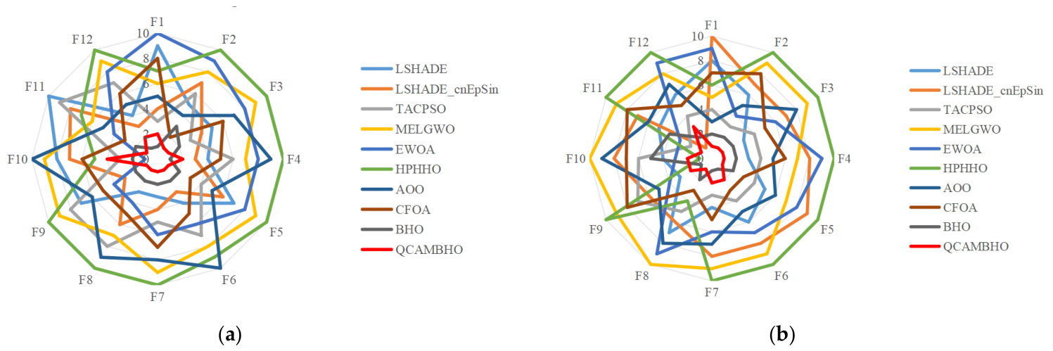
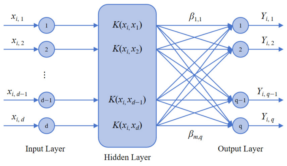
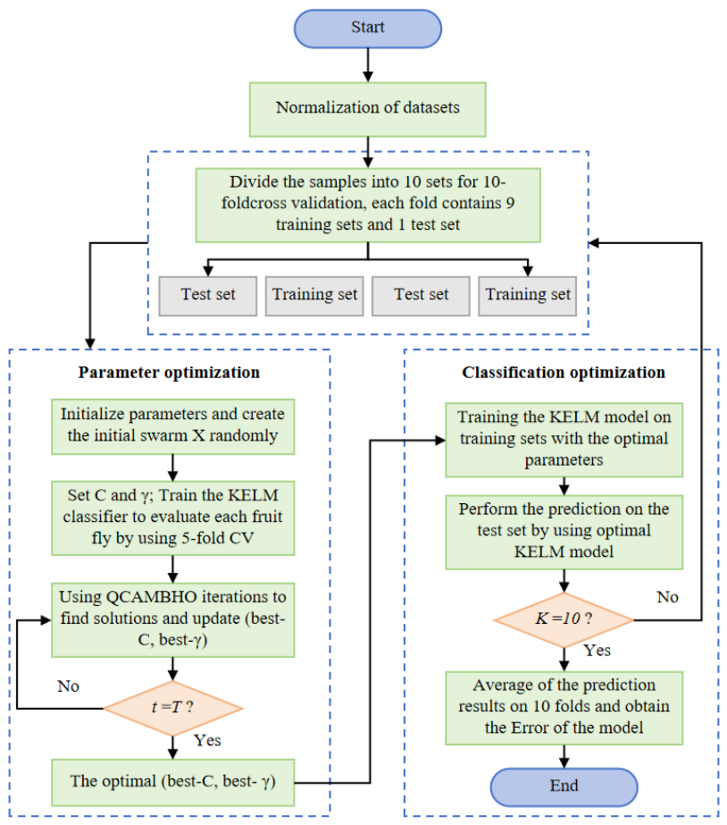
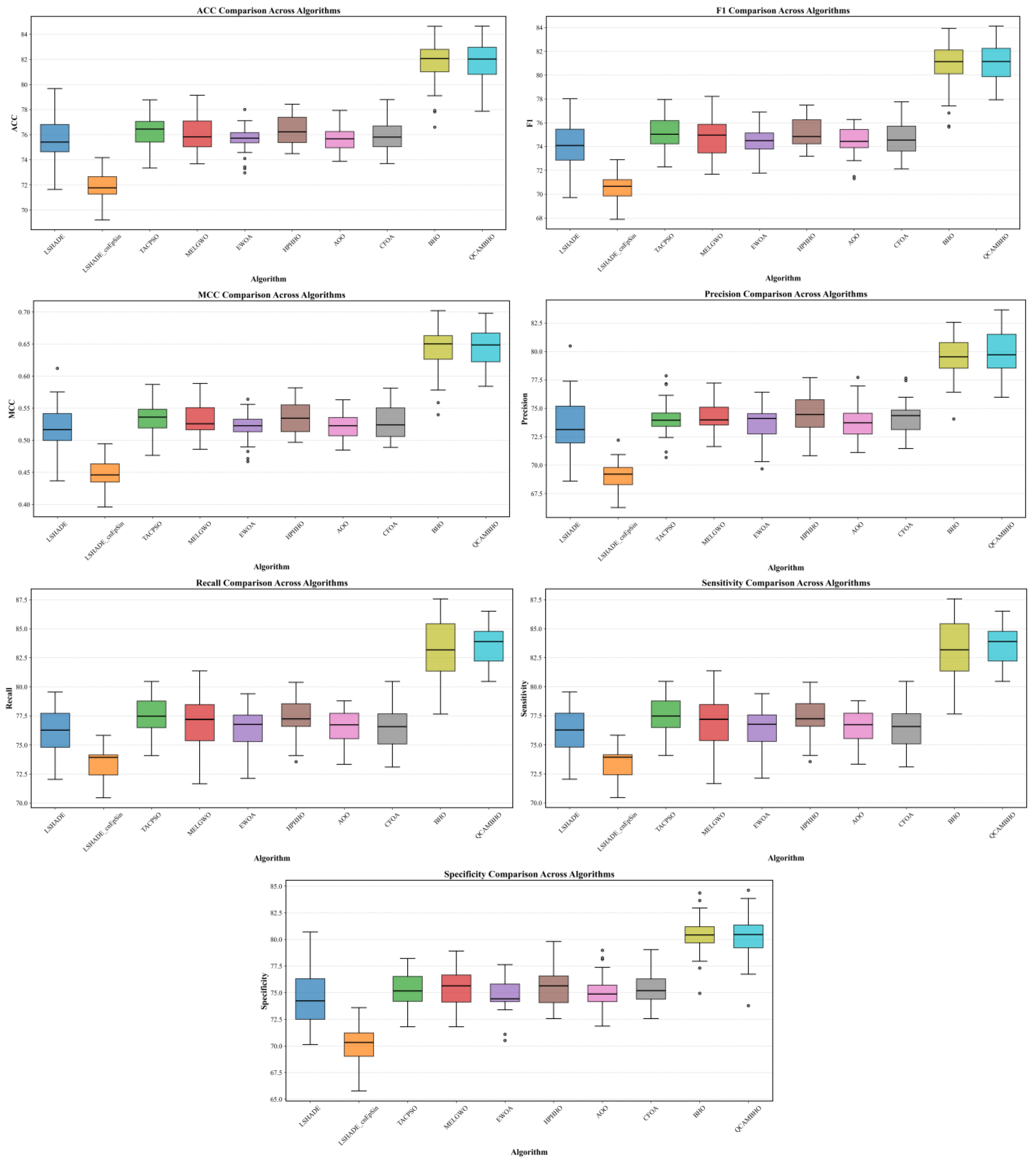
- Dual validation is conducted through numerical optimization and bankruptcy prediction. First, the numerical optimization performance of QCAMBHO is systematically evaluated on the CEC2017 and CEC2022 benchmark test functions. Its optimization capability is verified using the Wilcoxon rank-sum test, Friedman mean rank test, and convergence curve analysis. Furthermore, QCAMBHO is combined with the Kernel Extreme Learning Machine (KELM) to construct the QCAMBHO-KELM bankruptcy prediction model, which is used to optimize the key parameters of KELM. The predictive performance of the proposed model in financial classification tasks is evaluated using Accuracy, MCC, Sensitivity, Specificity, Precision, Recall, and F1-score.
2. Related Work
3. Materials and Methods
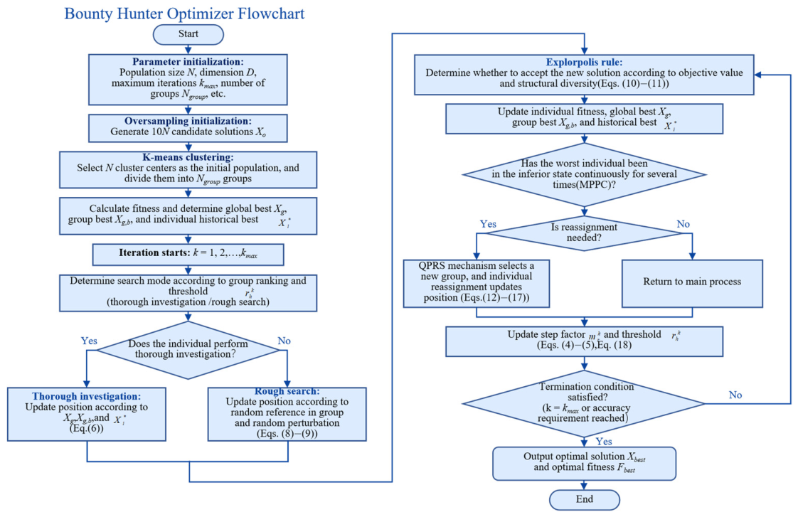
3.1. An Overview of BHO
- (1)
- Clustering Initialization
- (2)
- Adaptive Search Mode Switching
- (3)
- Fine Search Strategy
- (4)
- Rough Search Strategy
- (5)
- Explorpolis Rule
- (6)
- Inferior Individual Redistribution and QPRS Mechanism
3.2. Proposed QCAMBHO
3.2.1. Quantum-Computing-Enhanced Initialization Strategy
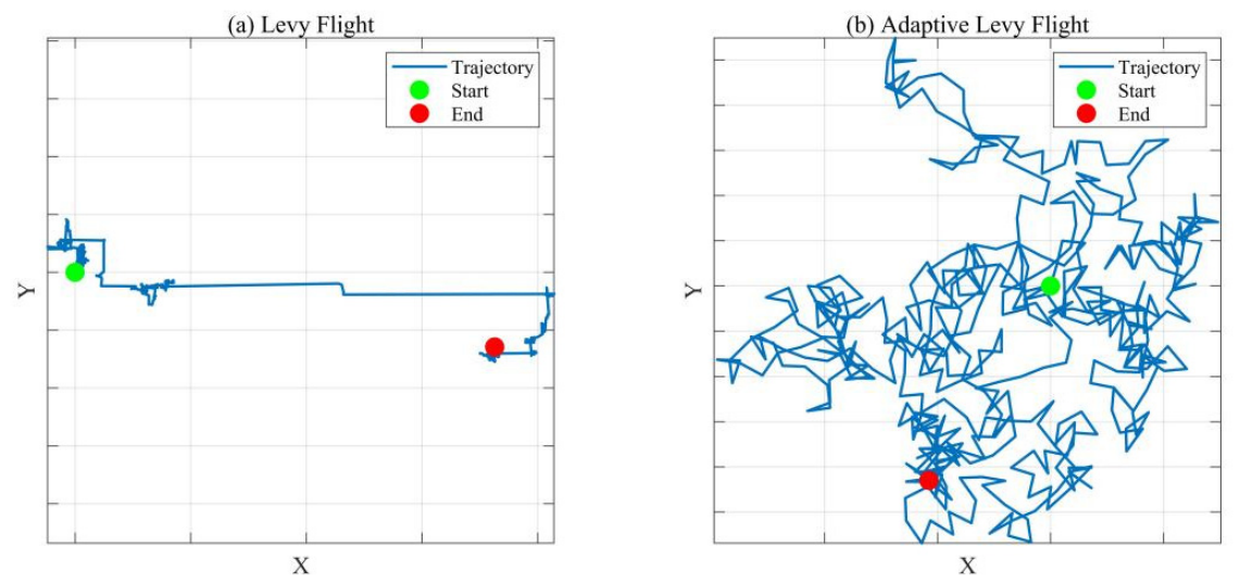
3.2.2. Adaptive Levy Flight Strategy
3.2.3. Adaptive Differential Operator
| Algorithm 1 QCAMBHO |
| Initialize population X by the standard BHO scheme via Equation (22) Enhance the initial population using quantum mapping and rotation via Equations (23)–(26) Evaluate fitness of all individuals and determine Set t = 1 while t ≤ T do Divide the population into elite individuals and explorer individuals for each individual do if is elite then Update by the original BHO exploitation mechanism else Replace the random disturbance in Rough Search with adaptive Levy flight Compute adaptive Levy weight via Equations (27)–(29) Update in Rough Search via Equations (30)–(31) end if Apply boundary control and greedy selection end for if t enters the late stage then Compute adaptive DE parameters F and CR via Equations (33) and (35) for each individual do Generate mutant vector via Equation (32) Generate trial vector via Equation (34) Update by greedy selection via Equation (36) end for end if Update and record Convergence(t); t = t + 1 end while return , Convergence |
3.3. Time Comparison Analysis of BHO and QCAMBHO
4. Numerical Experiments
4.1. CEC2017 and CEC2022 Test Suite
4.2. Algorithm Parameter Settings
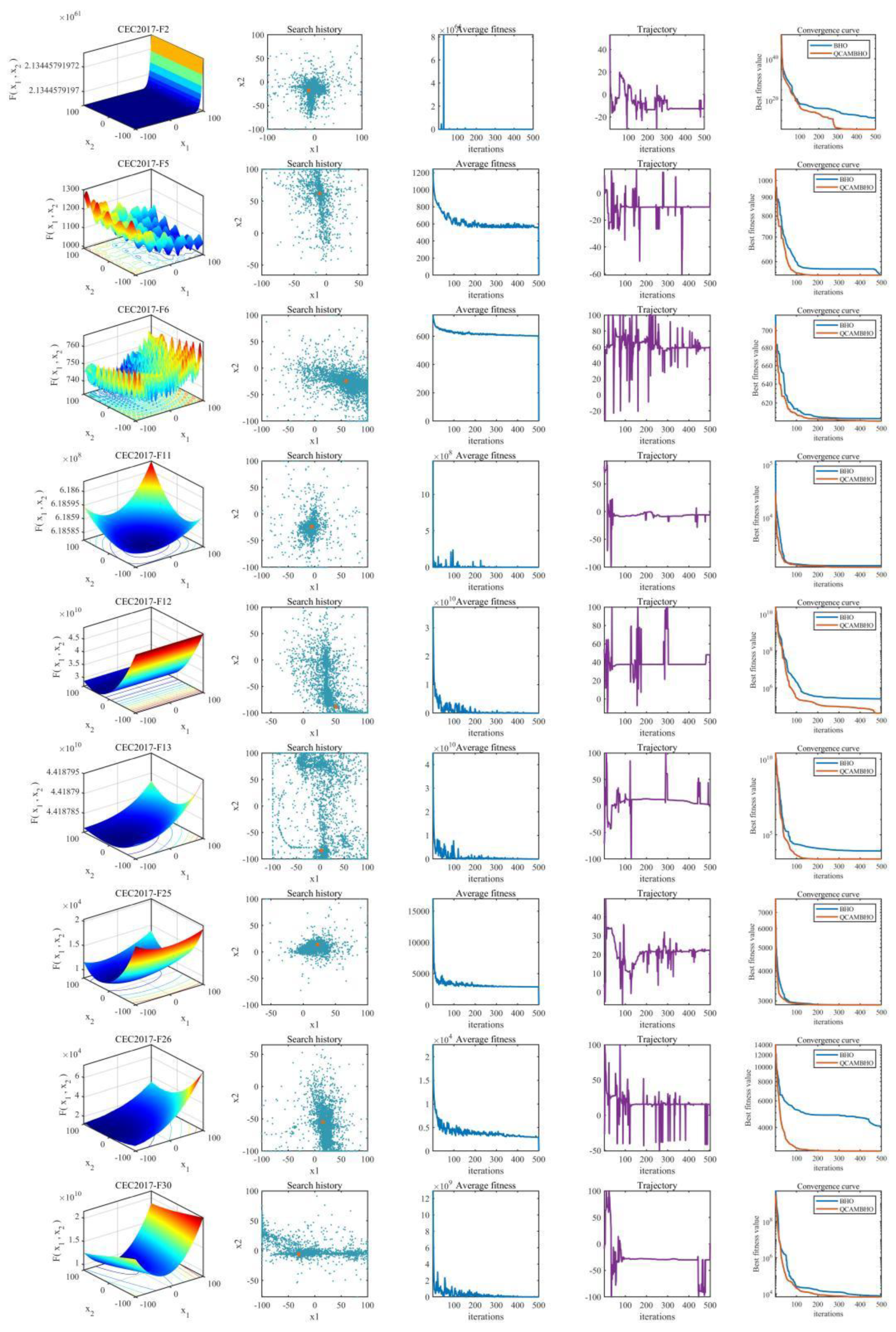
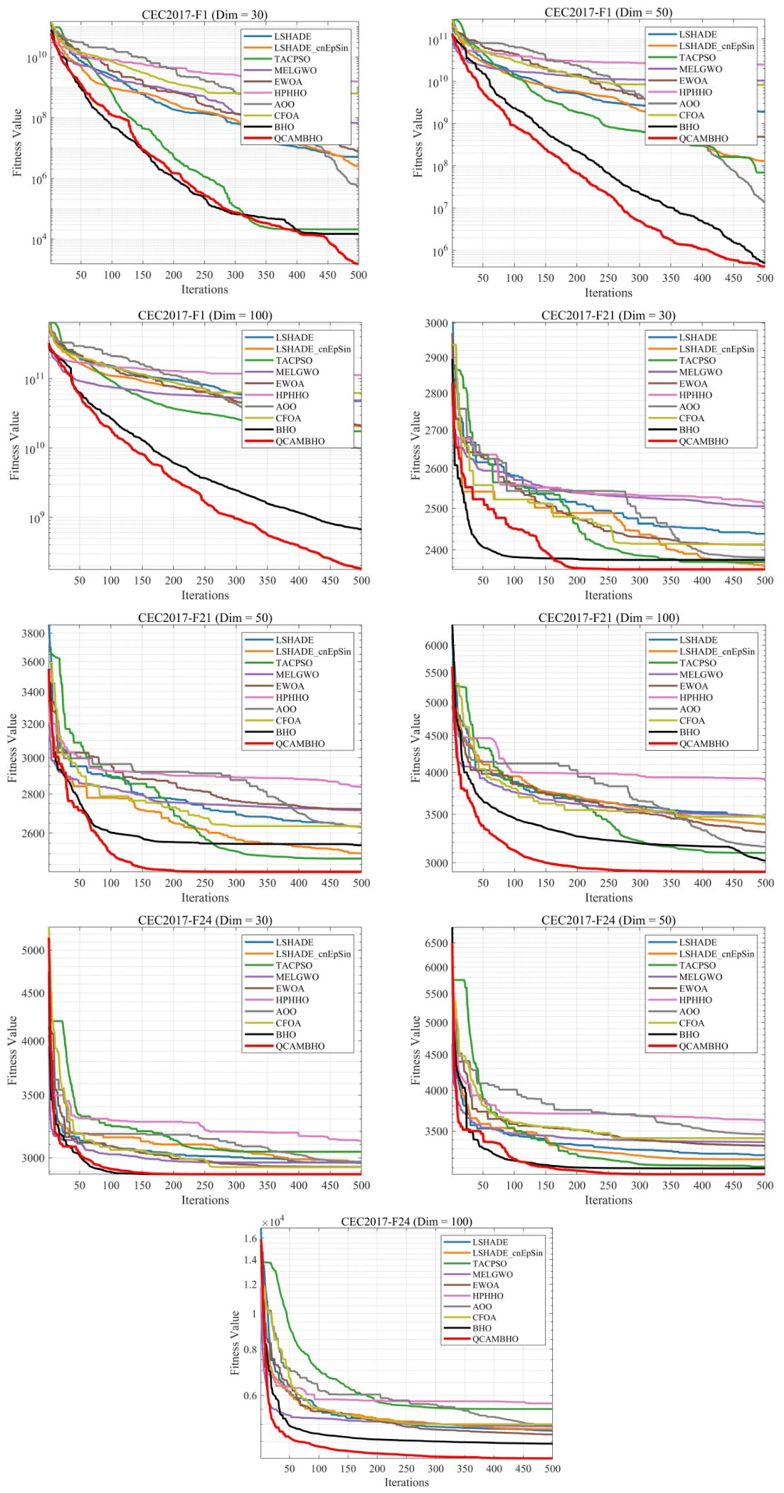
4.3. Convergence Behavior Evaluation
4.4. Quantitative Analysis
4.5. Ablation Experiment
4.6. Sensitivity Analysis
5. Bankruptcy Prediction Problem
5.1. QCAMBHO-KELM
5.2. Experimental Setup
5.3. Data Preprocessing and Experimental Settings
5.4. Measures for Performance Evaluation
5.5. Experimental Results and Analysis
6. Conclusions and Future Works
Author Contributions
Funding
Data Availability Statement
Conflicts of Interest
References
- Dasilas, A.; Rigani, A. Machine learning techniques in bankruptcy prediction: A systematic literature review. Expert Syst. Appl. 2024, 255, 124761. [Google Scholar] [CrossRef] [Scilit]
- Jones, S. A literature survey of corporate failure prediction models. J. Account. Lit. 2023, 45, 364–405. [Google Scholar] [CrossRef] [Scilit]
- El Madou, K.; Marso, S.; El Kharrim, M.; El Merouani, M. Evolutions in machine learning technology for financial distress prediction: A comprehensive review and comparative analysis. Expert Syst. 2024, 41, e13485. [Google Scholar] [CrossRef] [Scilit]
- Vásquez-Serpa, L.-J.; Rodríguez, C.; Pérez-Núñez, J.-R.; Navarro, C. Challenges of artificial intelligence for the prevention and identification of bankruptcy risk in financial institutions: A systematic review. J. Risk Financ. Manag. 2025, 18, 26. [Google Scholar] [CrossRef] [Scilit]
- Gnip, P.; Kanász, R.; Zoričak, M.; Drotár, P. An experimental survey of imbalanced learning algorithms for bankruptcy prediction. Artif. Intell. Rev. 2025, 58, 104. [Google Scholar] [CrossRef] [Scilit]
- Wang, X.; Kräussl, Z.; Brorsson, M. Datasets for advanced bankruptcy prediction: A survey and Taxonomy. arXiv 2024, arXiv:2411.01928. [Google Scholar] [CrossRef] [Scilit]
- Beaver, W.H. Financial ratios as predictors of failure. J. Account. Res. 1966, 4, 71–111. [Google Scholar] [CrossRef] [Scilit]
- Altman, E.I. Financial ratios, discriminant analysis and the prediction of corporate bankruptcy. J. Financ. 1968, 23, 589–609. [Google Scholar] [CrossRef]
- Altman, E.I.; Haldeman, R.G.; Narayanan, P. ZETATM analysis A new model to identify bankruptcy risk of corporations. J. Bank. Financ. 1977, 1, 29–54. [Google Scholar] [CrossRef] [Scilit]
- Ohlson, J.A. Financial ratios and the probabilistic prediction of bankruptcy. J. Account. Res. 1980, 18, 109–131. [Google Scholar] [CrossRef] [Scilit]
- Shumway, T. Forecasting bankruptcy more accurately: A simple hazard model. J. Bus. 2001, 74, 101–124. [Google Scholar] [CrossRef] [Scilit] [PubMed]
- Chava, S.; Jarrow, R.A. Bankruptcy prediction with industry effects. Rev. Financ. 2004, 8, 537–569. [Google Scholar] [CrossRef] [Scilit]
- Atiya, A.F. Bankruptcy prediction for credit risk using neural networks: A survey and new results. IEEE Trans. Neural Netw. 2001, 12, 929–935. [Google Scholar] [CrossRef] [Scilit] [PubMed]
- Verikas, A.; Kalsyte, Z.; Bacauskiene, M.; Gelzinis, A. Hybrid and ensemble-based soft computing techniques in bankruptcy prediction: A survey. Soft Comput. 2010, 14, 995–1010. [Google Scholar] [CrossRef] [Scilit]
- Barboza, F.; Kimura, H.; Altman, E. Machine learning models and bankruptcy prediction. Expert Syst. Appl. 2017, 83, 405–417. [Google Scholar] [CrossRef] [Scilit]
- Shi, Y.; Li, X. An overview of bankruptcy prediction models for corporate firms: A systematic literature review. Intang. Cap. 2019, 15, 114–127. [Google Scholar] [CrossRef] [Scilit]
- Qu, Y.; Quan, P.; Lei, M.; Shi, Y. Review of bankruptcy prediction using machine learning and deep learning techniques. Procedia Comput. Sci. 2019, 162, 895–899. [Google Scholar] [CrossRef] [Scilit]
- Li, Y.; Sun, K. Unleashing predicting a comparative study of machine learning for bankruptcy risk prediction. J. Artif. Intell. Syst. Model. 2024, 2, 99–113. [Google Scholar] [CrossRef]
- Pazouki, S.; Jamshidi, M.; Jalali, M.; Tafreshi, A. Artificial intelligence and digital technologies in finance: A comprehensive review. J. Econ. Financ. Account. Stud. 2025, 7, 54–69. [Google Scholar] [CrossRef] [Scilit]
- Naved, M.; Kumar, R.; Saheb, S.S. Analyzing financial stability by predicting bankruptcy situations with machine learning. J. Artif. Intell. Syst. Model. 2024, 2, 18–35. [Google Scholar] [CrossRef]
- Al Ali, A.; Khedr, A.M.; El Bannany, M.; Kanakkayil, S. GALSTM-FDP: A Time-Series Modeling Approach Using Hybrid GA and LSTM for Financial Distress Prediction. Int. J. Financ. Stud. 2023, 11, 38. [Google Scholar] [CrossRef] [Scilit]
- Kanász, R.; Gnip, P.; Zoričák, M.; Drotár, P. Bankruptcy prediction using ensemble of autoencoders optimized by genetic algorithm. PeerJ Comput. Sci. 2023, 9, e1257. [Google Scholar] [CrossRef] [Scilit] [PubMed]
- Ainan, U.H.; Por, L.Y.; Chen, Y.L.; Yang, J.; Ku, C.S. Advancing Bankruptcy Forecasting With Hybrid Machine Learning Techniques: Insights From an Unbalanced Polish Dataset. IEEE Access 2024, 12, 9369–9381. [Google Scholar] [CrossRef] [Scilit]
- Liu, J.; Wang, Z. Financial distress prediction using an improved particle swarm optimization wrapper feature selection method and tree boosting ensemble. J. Oper. Res. Soc. 2025, 76, 617–640. [Google Scholar] [CrossRef] [Scilit]
- Ezugwu, A.E.; Shukla, A.K.; Nath, R.; Akinyelu, A.A.; Agushaka, J.O.; Chiroma, H.; Muhuri, P.K. Metaheuristics: A comprehensive overview and classification along with bibliometric analysis. Artif. Intell. Rev. 2021, 54, 4237–4316. [Google Scholar] [CrossRef] [Scilit]
- Molina, D.; Poyatos, J.; Ser, J.D.; García, S.; Hussain, A.; Herrera, F. Comprehensive Taxonomies of Nature- and Bio-inspired Optimization: Inspiration Versus Algorithmic Behavior, Critical Analysis Recommendations. Cogn. Comput. 2020, 12, 897–939. [Google Scholar] [CrossRef] [Scilit]
- Deb, K. Genetic algorithm in search and optimization: The technique and applications. In Proceedings of International Workshop on Soft Computing and Intelligent Systems; ISI: Calcutta, India, 1998; pp. 58–87. [Google Scholar]
- Storn, R.; Price, K. Differential Evolution—A Simple and Efficient Heuristic for global Optimization over Continuous Spaces. J. Glob. Optim. 1997, 11, 341–359. [Google Scholar] [CrossRef] [Scilit]
- Dorigo, M.; Maniezzo, V.; Colorni, A. Ant system: Optimization by a colony of cooperating agents. IEEE Trans. Syst. Man Cybern. B Cybern. 1996, 26, 29–41. [Google Scholar] [CrossRef] [Scilit] [PubMed]
- Dorigo, M.; Birattari, M.; Stutzle, T. Ant colony optimization. IEEE Comput. Intell. Mag. 2006, 1, 28–39. [Google Scholar] [CrossRef] [Scilit]
- Dorigo, M.; Gambardella, L.M. Ant colony system: A cooperative learning approach to the traveling salesman problem. IEEE Trans. Evol. Comput. 1997, 1, 53–66. [Google Scholar] [CrossRef] [Scilit]
- Clerc, M.; Kennedy, J. The particle swarm—Explosion, stability, and convergence in a multidimensional complex space. IEEE Trans. Evol. Comput. 2002, 6, 58–73. [Google Scholar] [CrossRef] [Scilit]
- Kennedy, J.; Eberhart, R. Particle swarm optimization. In Proceedings of the ICNN’95—International Conference on Neural Networks, Perth, Australia, 27 November–1 December 1995; pp. 1942–1948. [Google Scholar] [CrossRef] [Scilit]
- Karaboga, D.; Basturk, B. A powerful and efficient algorithm for numerical function optimization: Artificial bee colony (ABC) algorithm. J. Glob. Optim. 2007, 39, 459–471. [Google Scholar] [CrossRef] [Scilit]
- Yang, X.S.; Suash, D. Cuckoo search via lévy flights. In Proceedings of the 2009 World Congress on Nature & Biologically Inspired Computing (NaBIC), Coimbatore, India, 9–11 December 2009; pp. 210–214. [Google Scholar] [CrossRef] [Scilit]
- Mirjalili, S.; Mirjalili, S.M.; Lewis, A. Grey wolf optimizer. Adv. Eng. Softw. 2014, 69, 46–61. [Google Scholar] [CrossRef] [Scilit]
- Mirjalili, S.; Lewis, A. The whale optimization algorithm. Adv. Eng. Softw. 2016, 95, 51–67. [Google Scholar] [CrossRef] [Scilit]
- Fu, S.; Li, K.; Huang, H.; Ma, C.; Fan, Q.; Zhu, Y. Red-billed blue magpie optimizer: A novel metaheuristic algorithm for 2D/3D UAV path planning and engineering design problems. Artif. Intell. Rev. 2024, 57, 134. [Google Scholar] [CrossRef] [Scilit]
- Yu, M.; Zhang, J.; Yu, L.; Yang, H.; Lu, H.; Wei, X.; Xu, J.J.A.I.R. Alzheimer’s disease brain image segmentation using multi-feature fusion in 3D Rényi entropy model and quantum hybrid optimization. Artif. Intell. Rev. 2026, 59, 95. [Google Scholar] [CrossRef] [Scilit]
- Yu, M.; Du, J.; Xu, X.; Xu, J.; Jiang, F.; Fu, S.; Zhang, J.; Liang, A.J.A.E.J. A multi-strategy enhanced Dung Beetle Optimization for real-world engineering problems and UAV path planning. Alex. Eng. J. 2025, 118, 406–434. [Google Scholar] [CrossRef] [Scilit]
- Yu, M.; Xu, J.; Liang, W.; Qiu, Y.; Bao, S.; Tang, L. Improved multi-strategy adaptive Grey Wolf Optimization for practical engineering applications and high-dimensional problem solving. Artif. Intell. Rev. 2024, 57, 277. [Google Scholar] [CrossRef] [Scilit]
- Fu, S.; Ma, C.; Li, K.; Xie, C.; Fan, Q.; Huang, H.; Xie, J.; Zhang, G.; Yu, M. Modified LSHADE-SPACMA with new mutation strategy and external archive mechanism for numerical optimization and point cloud registration. Artif. Intell. Rev. 2025, 58, 72. [Google Scholar] [CrossRef] [Scilit]
- Yu, M.; Yang, H.; Fu, S.; Kong, D.; Xu, X.; Zhang, J.; Xu, J. Improved Coverage and Redundancy Management in WSN Using ENMDBO: An Enhanced Metaheuristic Solution. IEEE Trans. Netw. Serv. Manag. 2025, 22, 5822–5839. [Google Scholar] [CrossRef] [Scilit]
- Brezočnik, L.; Fister, I.; Podgorelec, V. Swarm Intelligence Algorithms for Feature Selection: A Review. Appl. Sci. 2018, 8, 1521. [Google Scholar] [CrossRef] [Scilit]
- Agrawal, P.; Abutarboush, H.F.; Ganesh, T.; Mohamed, A.W. Metaheuristic Algorithms on Feature Selection: A Survey of One Decade of Research (2009–2019). IEEE Access 2021, 9, 26766–26791. [Google Scholar] [CrossRef] [Scilit]
- Yu, M.; Yang, H.; Zhang, J.; Ouyang, K.; Fu, S.; Tan, P.; Jiang, F.; Xu, J. Bounty hunter optimizer: A novel metaheuristic with an application to multi-UAV mobile edge computing and path planning. Knowl.-Based Syst. 2026, 341, 115836. [Google Scholar] [CrossRef] [Scilit]
- Sun, J.; Li, H.; Huang, Q.-H.; He, K.-Y. Predicting financial distress and corporate failure: A review from the state-of-the-art definitions, modeling, sampling, and featuring approaches. Knowl.-Based Syst. 2014, 57, 41–56. [Google Scholar] [CrossRef] [Scilit]
- Min, S.-H.; Lee, J.; Han, I. Combining genetic algorithms and support vector machines for banktruptcy prediction. In Korea Intelligent Information Systems Society; Korea Intelligent Information Systems Society: Seoul, Republic of Korea, 2004; pp. 179–188. [Google Scholar]
- Min, S.-H.; Lee, J.; Han, I. Hybrid genetic algorithms and support vector machines for bankruptcy prediction. Expert Syst. Appl. 2006, 31, 652–660. [Google Scholar] [CrossRef] [Scilit]
- Tsai, C.-F. Feature selection in bankruptcy prediction. Knowl.-Based Syst. 2009, 22, 120–127. [Google Scholar] [CrossRef] [Scilit]
- Chen, M.Y. A hybrid model for business failure prediction-utilization of particle swarm optimization and support vector machines. Neural Netw. World 2011, 21, 129–152. [Google Scholar] [CrossRef] [Scilit]
- Gao, R.; Cui, S.; Wang, Y.; Xu, W. Predicting financial distress in high-dimensional imbalanced datasets: A multi-heterogeneous self-paced ensemble learning framework. Financ. Innov. 2025, 11, 50. [Google Scholar] [CrossRef] [Scilit]
- Abror, W.F.; Alamsyah, A.; Aziz, M. Bankruptcy prediction using genetic algorithm-support vector machine (GA-SVM) feature selection and stacking. J. Inf. Syst. Explor. Res. 2023, 1. [Google Scholar] [CrossRef] [Scilit]
- Zainol, A.Z.; Saian, R.; Kin, T.Y.; Razali, M.H.M.; Bakar, S.A. An enhanced ant colony optimisation algorithm with the hellinger distance for shariah-compliant securities companies bankruptcy prediction. J. Inf. Commun. Technol. 2024, 23, 1–24. [Google Scholar] [CrossRef] [Scilit]
- Yang, L. Enterprise Financial Risk Early Warning Prediction using Tuna Swarm Optimization Algorithm with Xg boost Model. In Proceedings of the 2024 International Conference on Distributed Systems, Computer Networks and Cybersecurity (ICDSCNC), Bengaluru, India, 20–21 September 2024; pp. 1–5. [Google Scholar] [CrossRef] [Scilit]
- Ji, Y.; Lu, C.; Liu, L.; Heidari, A.A.; Wu, C.; Chen, H. Advancing bankruptcy prediction: A study on an improved rime optimization algorithm and its application in feature selection. Int. J. Mach. Learn. Cybern. 2025, 16, 3461–3499. [Google Scholar] [CrossRef] [Scilit]
- Abdullayev, I.; Akhmetshin, E.; Kosorukova, I.; Klochko, E.; Cho, W.; Joshi, G.P. Modeling of extended osprey optimization algorithm with Bayesian neural network: An application on Fintech to predict financial crisis. AIMS Math. 2024, 9, 17555–17577. [Google Scholar] [CrossRef] [Scilit]
- Sherov, A.; Rakhimov, T.; Hajiyev, H.; Zelinskaya, M.; Khidirova, G. Evaluating Class-Imbalanced Data Handling for Enhanced Financial Distress Prediction Using an Attention-Based Deep Neural Network and Heuristic Optimization Algorithms. Eng. Technol. Appl. Sci. Res. 2025, 15, 28862–28867. [Google Scholar] [CrossRef] [Scilit]
- Sherov, A.; Rakhimov, T.; Hajiyev, H.; Zelinskaya, M.; Khidirova, G. Assessment of Class Imbalance Data Handling with Attention-Based Deep Learning Approach for Robust Financial Distress Prediction in Enterprises. Eng. Technol. Appl. Sci. Res. 2025, 15, 30053–30058. [Google Scholar] [CrossRef] [Scilit]
- Yotsawat, W.; Phodong, K.; Promrat, T.; Wattuya, P. Bankruptcy prediction model using cost-sensitive extreme gradient boosting in the context of imbalanced datasets. Int. J. Electr. Comput. Eng. 2023, 13, 4683–4691. [Google Scholar] [CrossRef] [Scilit]
- Tanabe, R.; Fukunaga, A.S. Improving the search performance of SHADE using linear population size reduction. In Proceedings of the 2014 IEEE Congress on Evolutionary Computation (CEC), Beijing, China, 6–11 July 2014; pp. 1658–1665. [Google Scholar] [CrossRef] [Scilit]
- Awad, N.H.; Ali, M.Z.; Suganthan, P.N. Ensemble sinusoidal differential covariance matrix adaptation with Euclidean neighborhood for solving CEC2017 benchmark problems. In Proceedings of the 2017 IEEE Congress on Evolutionary Computation (CEC), San Sebastian, Spain, 5–8 June 2017; pp. 372–379. [Google Scholar] [CrossRef] [Scilit]
- Ratnaweera, A.; Halgamuge, S.K.; Watson, H.C. Self-organizing hierarchical particle swarm optimizer with time-varying acceleration coefficients. IEEE Trans. Evol. Comput. 2004, 8, 240–255. [Google Scholar] [CrossRef] [Scilit]
- Ahmed, R.; Rangaiah, G.P.; Mahadzir, S.; Mirjalili, S.; Hassan, M.H.; Kamel, S. Memory, evolutionary operator, and local search based improved Grey Wolf Optimizer with linear population size reduction technique. Knowl.-Based Syst. 2023, 264, 110297. [Google Scholar] [CrossRef] [Scilit]
- Cao, D.; Xu, Y.; Yang, Z.; Dong, H.; Li, X. An enhanced whale optimization algorithm with improved dynamic opposite learning and adaptive inertia weight strategy. Complex Intell. Syst. 2023, 9, 767–795. [Google Scholar] [CrossRef] [Scilit]
- Su, Y.; Dai, Y.; Liu, Y. A hybrid parallel Harris hawks optimization algorithm for reusable launch vehicle reentry trajectory optimization with no-fly zones. Soft Comput. 2021, 25, 14597–14617. [Google Scholar] [CrossRef] [Scilit]
- Wang, R.-B.; Hu, R.-B.; Geng, F.-D.; Xu, L.; Chu, S.-C.; Pan, J.-S.; Meng, Z.-Y.; Mirjalili, S. The Animated Oat Optimization Algorithm: A nature-inspired metaheuristic for engineering optimization and a case study on Wireless Sensor Networks. Knowl.-Based Syst. 2025, 318, 113589. [Google Scholar] [CrossRef] [Scilit]
- Jia, H.; Wen, Q.; Wang, Y.; Mirjalili, S. Catch fish optimization algorithm: A new human behavior algorithm for solving clustering problems. Clust. Comput. 2024, 27, 13295–13332. [Google Scholar] [CrossRef] [Scilit]
- Zhao, D.; Huang, C.; Wei, Y.; Yu, F.; Wang, M.; Chen, H. An effective computational model for bankruptcy prediction using kernel extreme learning machine approach. Comput. Econ. 2017, 49, 325–341. [Google Scholar] [CrossRef] [Scilit]
- Wang, M.; Chen, H.; Li, H.; Cai, Z.; Zhao, X.; Tong, C.; Li, J.; Xu, X. Grey wolf optimization evolving kernel extreme learning machine: Application to bankruptcy prediction. Eng. Appl. Artif. Intell. 2017, 63, 54–68. [Google Scholar] [CrossRef] [Scilit]
- Liu, W.; Wu, H.; Wang, T.; Wu, H. Elite elimination osprey optimization algorithm optimized kernel extreme learning machine for bankruptcy prediction problems. Sci. Rep. 2026, 16, 6246. [Google Scholar] [CrossRef] [Scilit] [PubMed]
- Liu, W.; Zhang, Y.; Du, M. Enhanced adaptive zebra optimization algorithm optimized kernel extreme learning machine for bankruptcy prediction problems. Sci. Rep. 2026, 16, 10268. [Google Scholar] [CrossRef] [Scilit] [PubMed]





| Algorithm | F1 | F2 | F3 | F4 | F5 | F6 |
|---|---|---|---|---|---|---|
| BHO | 5.0032 | 4.4125 | 3.9555 | 4.2645 | 4.0743 | 5.3194 |
| QCAMBHO | 5.8721 | 5.4189 | 4.7558 | 5.2820 | 5.9945 | 5.9778 |
| Algorithm | F7 | F8 | F9 | F10 | F11 | F12 |
| BHO | 4.3566 | 4.2716 | 4.3799 | 4.4405 | 4.1313 | 4.5465 |
| QCAMBHO | 5.7317 | 6.1479 | 5.3691 | 4.8209 | 5.0039 | 5.5258 |
| Algorithm | F13 | F14 | F15 | F16 | F17 | F18 |
| BHO | 4.3542 | 4.9157 | 4.2170 | 3.8678 | 4.6570 | 4.5148 |
| QCAMBHO | 4.8265 | 5.3637 | 5.0689 | 5.4596 | 5.8412 | 5.6948 |
| Algorithm | F19 | F20 | F21 | F22 | F23 | F24 |
| BHO | 5.6267 | 4.5516 | 4.5398 | 5.1230 | 5.2220 | 5.0927 |
| QCAMBHO | 6.7014 | 5.8220 | 5.8578 | 6.7054 | 6.1835 | 6.2793 |
| Algorithm | F25 | F26 | F27 | F28 | F29 | F30 |
| BHO | 1.9526 | 2.3578 | 2.9199 | 2.3202 | 2.0432 | 2.3255 |
| QCAMBHO | 2.5756 | 3.1621 | 3.5482 | 2.9974 | 2.5686 | 3.0160 |
| Type | ID | Description | Dim | fmin |
|---|---|---|---|---|
| Unimodal | F1 | Shifted and Rotated Bent Cigar Function | 30/50/100 | 100 |
| F2 | Shifted and Rotated Sum of Different Power Function | 30/50/100 | 200 | |
| F3 | Shifted and Rotated Zakharov Function | 30/50/100 | 300 | |
| Multimodal | F4 | Shifted and Rotated Rosenbrock’s Function | 30/50/100 | 400 |
| F5 | Shifted and Rotated Rastrigin’s Function | 30/50/100 | 500 | |
| F6 | Shifted and Rotated Expanded Scaffer’s F6 Function | 30/50/100 | 600 | |
| F7 | Shifted and Rotated Lunacek Bi_Rastrigin Function | 30/50/100 | 700 | |
| F8 | Shifted and Rotated Non-Continuous Rastrigin’s Function | 30/50/100 | 800 | |
| F9 | Shifted and Rotated Levy Function | 30/50/100 | 900 | |
| F10 | Shifted and Rotated Schwefel’s Function | 30/50/100 | 1000 | |
| Hybrid | F11 | Hybrid Function 1 (N = 3) | 30/50/100 | 1100 |
| F12 | Hybrid Function 2 (N = 3) | 30/50/100 | 1200 | |
| F13 | Hybrid Function 3 (N = 3) | 30/50/100 | 1300 | |
| F14 | Hybrid Function 6 (N = 4) | 30/50/100 | 1400 | |
| F15 | Hybrid Function 6 (N = 4) | 30/50/100 | 1500 | |
| F16 | Hybrid Function 6 (N = 4) | 30/50/100 | 1600 | |
| F17 | Hybrid Function 6 (N = 5) | 30/50/100 | 1700 | |
| F18 | Hybrid Function 6 (N = 5) | 30/50/100 | 1800 | |
| F19 | Hybrid Function 6 (N = 5) | 30/50/100 | 1900 | |
| F20 | Hybrid Function 6 (N = 6) | 30/50/100 | 2000 | |
| Composition | F21 | Composition Function 1 (N = 5) | 30/50/100 | 2100 |
| F22 | Composition Function 2 (N = 5) | 30/50/100 | 2200 | |
| F23 | Composition Function 3 (N = 5) | 30/50/100 | 2300 | |
| F24 | Composition Function 4 (N = 5) | 30/50/100 | 2400 | |
| F25 | Composition Function 5 (N = 3) | 30/50/100 | 2500 | |
| F26 | Composition Function 6 (N = 3) | 30/50/100 | 2600 | |
| F27 | Composition Function 7 (N = 5) | 30/50/100 | 2700 | |
| F28 | Composition Function 8 (N = 5) | 30/50/100 | 2800 | |
| F29 | Composition Function 9 (N = 5) | 30/50/100 | 2900 | |
| F30 | Composition Function 10 (N = 3) | 30/50/100 | 3000 | |
| Search Range: [−100, 100] in each dimension |
| Type | ID | Description | Dim | fmin |
|---|---|---|---|---|
| Unimodal Function | F1 | Shifted and full Rotated Zakharov Function | 10/20 | 300 |
| Basic Functions | F2 | Shifted and full Rotated Zakharov Function | 10/20 | 400 |
| F3 | Shifted and full Rotated Expanded Schaffer’s f6 Function | 10/20 | 600 | |
| F4 | Shifted and full Rotated Non-Continuous Rastrigin’s Function | 10/20 | 800 | |
| F5 | Shifted and full Rotated Levy Function | 10/20 | 900 | |
| Hybrid Functions | F6 | Hybrid Function 1 (N = 3) | 10/20 | 1800 |
| F7 | Hybrid Function 2 (N = 6) | 10/20 | 2000 | |
| F8 | Hybrid Function 3 (N = 5) | 10/20 | 2200 | |
| Composition Functions | F9 | Composition Function 1 (N = 5) | 10/20 | 2300 |
| F10 | Composition Function 2 (N = 4) | 10/20 | 2400 | |
| F11 | Composition Function 3 (N = 5) | 10/20 | 2600 | |
| F12 | Composition Function 4 (N = 6) | 10/20 | 2700 | |
| Search Range: [−100, 100] in each dimension |
| Algorithms | Name of the Parameter | Value of the Parameter |
|---|---|---|
| LSHADE | (0.11, 6, 4) | |
| LSHADE_cnEpSin | (0.11, 5, 1.4) | |
| TACPSO | (0.9, 0.4, 2.5, 0.5, 0.5, 2.5) | |
| MELGWO | 10; linearly decreases from 2 to 0; 2 | |
| EWOA | ||
| HPHHO | [−1, 1] | |
| AOO | [0, 1] | |
| CFOA | [−1, 1] | |
| BHO | [0, 1] | |
| QCAMBHO | [0, 1] |
| Algorithm | Metric | LSHADE | LSHADE_cnEpSin | TACPSO | MELGWO | EWOA | HPHHO | AOO | CFOA | BHO | QCAMBHO |
|---|---|---|---|---|---|---|---|---|---|---|---|
| F1 | Mean | 4.8022 × 10⁷ | 6.0805 × 10⁶ | 3.4471 × 10⁷ | 1.9155 × 10⁹ | 1.6091 × 10⁷ | 2.4203 × 10⁹ | 1.0997 × 10⁶ | 6.0332 × 10⁸ | 5.8989 × 10³ | 4.8457 × 10³ |
| Std | 9.7965 × 10⁷ | 8.1445 × 10⁶ | 1.8743 × 10⁸ | 2.2546 × 10⁹ | 2.2751 × 10⁷ | 1.2267 × 10⁹ | 5.8875 × 10⁵ | 2.2917 × 10⁸ | 5.3220 × 10³ | 5.5971 × 10³ | |
| F2 | Mean | 2.9524 × 1027 | 4.9061 × 1026 | 6.2854 × 1029 | 1.9238 × 1031 | 4.1165 × 1024 | 1.0000 × 10²⁰ | 2.3149 × 10²⁰ | 2.7467 × 1027 | 1.9863 × 10¹⁴ | 9.5753 × 10¹⁰ |
| Std | 1.1279 × 1028 | 2.5908 × 1027 | 3.2751 × 1030 | 7.6875 × 1031 | 1.2527 × 1025 | 0.0000 × 100 | 1.0153 × 10²¹ | 1.4223 × 1028 | 5.7370 × 10¹⁴ | 3.3544 × 10¹¹ | |
| F3 | Mean | 9.6977 × 10⁴ | 5.9049 × 10⁴ | 5.1553 × 10⁴ | 4.2094 × 10⁴ | 1.0311 × 10⁵ | 4.6948 × 10⁴ | 3.7896 × 10⁴ | 5.4033 × 10⁴ | 4.5648 × 10³ | 3.6069 × 10³ |
| Std | 5.3581 × 10⁴ | 3.5283 × 10⁴ | 1.7264 × 10⁴ | 1.0640 × 10⁴ | 2.1922 × 10⁴ | 8.3967 × 10³ | 1.3405 × 10⁴ | 9.9604 × 10³ | 2.2541 × 10³ | 1.9662 × 10³ | |
| F4 | Mean | 5.5408 × 10² | 5.3857 × 10² | 5.3009 × 10² | 6.5865 × 10² | 5.3510 × 10² | 8.1201 × 10² | 5.1798 × 10² | 6.2978 × 10² | 4.9578 × 10² | 4.8149 × 10² |
| Std | 6.0484 × 101 | 3.9164 × 101 | 5.5115 × 101 | 1.8043 × 10² | 3.9452 × 101 | 1.7037 × 10² | 2.2008 × 101 | 5.6390 × 101 | 1.8219 × 101 | 2.6849 × 101 | |
| F5 | Mean | 6.1258 × 10² | 6.0133 × 10² | 6.0276 × 10² | 6.7015 × 10² | 6.6782 × 10² | 7.8008 × 10² | 6.3763 × 10² | 6.6931 × 10² | 5.6022 × 10² | 5.6514 × 10² |
| Std | 2.5796 × 101 | 2.2214 × 101 | 2.6386 × 101 | 3.4348 × 101 | 4.3927 × 101 | 3.0665 × 101 | 3.0092 × 101 | 2.3832 × 101 | 1.3392 × 101 | 1.5185 × 101 | |
| F6 | Mean | 6.0879 × 10² | 6.1271 × 10² | 6.1202 × 10² | 6.4400 × 10² | 6.3067 × 10² | 6.5999 × 10² | 6.3219 × 10² | 6.2942 × 10² | 6.0373 × 10² | 6.0226 × 10² |
| Std | 6.5409 × 100 | 5.1840 × 100 | 6.0664 × 100 | 9.8154 × 100 | 1.0828 × 101 | 8.6766 × 100 | 1.1630 × 101 | 8.4611 × 100 | 1.6262 × 100 | 1.4748 × 100 | |
| F7 | Mean | 9.4564 × 10² | 9.1224 × 10² | 8.5139 × 10² | 1.0027 × 10³ | 1.0057 × 10³ | 1.2263 × 10³ | 8.9202 × 10² | 9.6708 × 10² | 8.0888 × 10² | 7.9369 × 10² |
| Std | 6.4993 × 101 | 4.4254 × 101 | 3.8823 × 101 | 6.9371 × 101 | 6.5324 × 101 | 9.1440 × 101 | 3.0547 × 101 | 4.3529 × 101 | 2.1067 × 101 | 2.5416 × 101 | |
| F8 | Mean | 9.0492 × 10² | 9.0511 × 10² | 8.9964 × 10² | 9.3858 × 10² | 9.5073 × 10² | 1.0115 × 10³ | 9.0656 × 10² | 9.4894 × 10² | 8.5929 × 10² | 8.5993 × 10² |
| Std | 2.2848 × 101 | 2.1158 × 101 | 2.6475 × 101 | 2.9309 × 101 | 3.6052 × 101 | 2.2197 × 101 | 3.0335 × 101 | 2.2613 × 101 | 2.3165 × 101 | 1.5099 × 101 | |
| F9 | Mean | 2.9824 × 10³ | 2.2788 × 10³ | 2.8435 × 10³ | 3.6346 × 10³ | 4.6715 × 10³ | 6.3461 × 10³ | 3.9938 × 10³ | 2.6184 × 10³ | 1.2711 × 10³ | 1.1146 × 10³ |
| Std | 1.3500 × 10³ | 4.5784 × 10² | 1.5866 × 10³ | 6.2137 × 10² | 1.7759 × 10³ | 9.5490 × 10² | 1.4814 × 10³ | 8.2234 × 10² | 2.7136 × 10² | 1.1979 × 10² | |
| F10 | Mean | 4.8856 × 10³ | 5.1589 × 10³ | 5.1197 × 10³ | 5.0617 × 10³ | 6.3405 × 10³ | 6.1930 × 10³ | 4.8202 × 10³ | 6.8864 × 10³ | 4.6953 × 10³ | 4.3927 × 10³ |
| Std | 4.6370 × 10² | 8.7415 × 10² | 6.9352 × 10² | 6.3968 × 10² | 1.2478 × 10³ | 4.4510 × 10² | 7.2161 × 10² | 5.6063 × 10² | 4.8875 × 10² | 6.4551 × 10² | |
| F11 | Mean | 1.7826 × 10³ | 1.3395 × 10³ | 1.2987 × 10³ | 1.4369 × 10³ | 1.3746 × 10³ | 1.6530 × 10³ | 1.2980 × 10³ | 1.5706 × 10³ | 1.2129 × 10³ | 1.1955 × 10³ |
| Std | 1.4634 × 10³ | 7.7573 × 101 | 7.0218 × 101 | 1.9091 × 10² | 9.6230 × 101 | 1.4148 × 10² | 5.0164 × 101 | 1.5902 × 10² | 3.6187 × 101 | 3.9034 × 101 | |
| F12 | Mean | 2.7598 × 10⁶ | 2.9897 × 10⁶ | 1.4960 × 10⁶ | 4.4103 × 10⁷ | 3.6024 × 10⁶ | 2.0892 × 10⁸ | 1.8541 × 10⁷ | 3.2656 × 10⁷ | 2.1427 × 10⁵ | 1.0313 × 10⁵ |
| Std | 4.3171 × 10⁶ | 3.7448 × 10⁶ | 2.6151 × 10⁶ | 6.8810 × 10⁷ | 2.4532 × 10⁶ | 1.4609 × 10⁸ | 1.3919 × 10⁷ | 1.7685 × 10⁷ | 1.7728 × 10⁵ | 1.4519 × 10⁵ | |
| F13 | Mean | 1.5133 × 10⁴ | 3.6528 × 10⁴ | 1.7096 × 10⁵ | 1.2651 × 10⁵ | 1.5008 × 10⁴ | 4.3054 × 10⁶ | 1.2650 × 10⁵ | 4.2069 × 10⁴ | 1.0033 × 10⁴ | 2.4161 × 10³ |
| Std | 1.8746 × 10⁴ | 2.0587 × 10⁴ | 8.1342 × 10⁵ | 1.1810 × 10⁵ | 1.2257 × 10⁴ | 5.9205 × 10⁶ | 1.4656 × 10⁵ | 1.9778 × 10⁴ | 1.0943 × 10⁴ | 7.9642 × 10² | |
| F14 | Mean | 1.1605 × 10⁵ | 3.0324 × 10³ | 3.1829 × 10⁴ | 1.8148 × 10⁵ | 2.2540 × 10⁵ | 6.8481 × 10⁵ | 1.1468 × 10⁵ | 1.9619 × 10⁴ | 1.5907 × 10³ | 1.5896 × 10³ |
| Std | 5.4852 × 10⁵ | 2.1365 × 10³ | 2.9070 × 10⁴ | 2.1355 × 10⁵ | 2.5538 × 10⁵ | 7.1608 × 10⁵ | 8.8586 × 10⁴ | 2.0831 × 10⁴ | 6.8706 × 101 | 5.4482 × 101 | |
| F15 | Mean | 1.2477 × 10⁴ | 1.0745 × 10⁴ | 8.6916 × 10³ | 2.9062 × 10⁴ | 8.6703 × 10³ | 1.1393 × 10⁵ | 5.2360 × 10⁴ | 2.6446 × 10⁴ | 2.1362 × 10³ | 1.7535 × 10³ |
| Std | 9.3342 × 10³ | 1.0372 × 10⁴ | 8.6563 × 10³ | 1.8199 × 10⁴ | 6.8605 × 10³ | 1.6172 × 10⁵ | 3.2223 × 10⁴ | 1.4898 × 10⁴ | 2.2189 × 10² | 1.4981 × 10² | |
| F16 | Mean | 2.7406 × 10³ | 2.5670 × 10³ | 2.6460 × 10³ | 2.8758 × 10³ | 2.8691 × 10³ | 3.3267 × 10³ | 2.8248 × 10³ | 2.7232 × 10³ | 2.2159 × 10³ | 2.1486 × 10³ |
| Std | 3.1318 × 10² | 2.1476 × 10² | 2.3298 × 10² | 3.5703 × 10² | 3.4904 × 10² | 4.0218 × 10² | 3.2850 × 10² | 2.0900 × 10² | 1.9062 × 10² | 2.1504 × 10² | |
| F17 | Mean | 2.2137 × 10³ | 2.0376 × 10³ | 2.1884 × 10³ | 2.2279 × 10³ | 2.3784 × 10³ | 2.4720 × 10³ | 2.1993 × 10³ | 2.0662 × 10³ | 1.8579 × 10³ | 1.8581 × 10³ |
| Std | 2.1439 × 10² | 1.5562 × 10² | 2.0512 × 10² | 2.5638 × 10² | 2.9463 × 10² | 2.1867 × 10² | 1.9367 × 10² | 1.4268 × 10² | 6.5249 × 101 | 1.0123 × 10² | |
| F18 | Mean | 4.1152 × 10⁵ | 1.6058 × 10⁵ | 2.3487 × 10⁵ | 1.3946 × 10⁶ | 1.5532 × 10⁶ | 3.1271 × 10⁶ | 1.1949 × 10⁶ | 2.2572 × 10⁵ | 2.6050 × 10⁴ | 2.8504 × 10⁴ |
| Std | 1.2211 × 10⁶ | 2.9007 × 10⁵ | 1.6044 × 10⁵ | 1.2666 × 10⁶ | 1.7523 × 10⁶ | 2.3537 × 10⁶ | 2.0154 × 10⁶ | 2.6940 × 10⁵ | 1.8043 × 10⁴ | 2.6019 × 10⁴ | |
| F19 | Mean | 1.2146 × 10⁴ | 8.5549 × 10³ | 1.1455 × 10⁴ | 8.2827 × 10⁴ | 1.0087 × 10⁴ | 1.5339 × 10⁶ | 6.6527 × 10⁵ | 2.0019 × 10⁵ | 2.1326 × 10³ | 2.0831 × 10³ |
| Std | 1.2089 × 10⁴ | 1.0027 × 10⁴ | 2.0272 × 10⁴ | 1.1696 × 10⁵ | 1.1514 × 10⁴ | 1.9760 × 10⁶ | 6.3862 × 10⁵ | 3.2320 × 10⁵ | 9.5279 × 101 | 6.8725 × 101 | |
| F20 | Mean | 2.5287 × 10³ | 2.3903 × 10³ | 2.5340 × 10³ | 2.6433 × 10³ | 2.6314 × 10³ | 2.6374 × 10³ | 2.5454 × 10³ | 2.4305 × 10³ | 2.2386 × 10³ | 2.1918 × 10³ |
| Std | 1.6940 × 10² | 1.2541 × 10² | 2.0607 × 10² | 1.9636 × 10² | 1.6124 × 10² | 1.7675 × 10² | 1.8158 × 10² | 1.2854 × 10² | 9.5825 × 101 | 9.0232 × 101 | |
| F21 | Mean | 2.4082 × 10³ | 2.3986 × 10³ | 2.3862 × 10³ | 2.4541 × 10³ | 2.4342 × 10³ | 2.5450 × 10³ | 2.4252 × 10³ | 2.4412 × 10³ | 2.3598 × 10³ | 2.3586 × 10³ |
| Std | 1.8896 × 101 | 1.8354 × 101 | 1.8887 × 101 | 3.4359 × 101 | 3.3797 × 101 | 5.4605 × 101 | 3.3491 × 101 | 2.3677 × 101 | 1.9108 × 101 | 1.5761 × 101 | |
| F22 | Mean | 3.4119 × 10³ | 4.2492 × 10³ | 3.8675 × 10³ | 5.4897 × 10³ | 2.3289 × 10³ | 5.6480 × 10³ | 5.1990 × 10³ | 2.6277 × 10³ | 2.3013 × 10³ | 2.3006 × 10³ |
| Std | 1.6849 × 10³ | 2.3886 × 10³ | 1.8980 × 10³ | 2.0491 × 10³ | 1.2089 × 101 | 2.5051 × 10³ | 2.1560 × 10³ | 5.3530 × 10² | 1.9783 × 100 | 1.2187 × 100 | |
| F23 | Mean | 2.7930 × 10³ | 2.7739 × 10³ | 2.7791 × 10³ | 2.8483 × 10³ | 2.8096 × 10³ | 2.9796 × 10³ | 2.8162 × 10³ | 2.8146 × 10³ | 2.7261 × 10³ | 2.7262 × 10³ |
| Std | 5.0992 × 101 | 3.8697 × 101 | 3.5745 × 101 | 5.4939 × 101 | 4.7489 × 101 | 9.7586 × 101 | 4.2735 × 101 | 3.0064 × 101 | 2.3523 × 101 | 2.1862 × 101 | |
| F24 | Mean | 2.9456 × 10³ | 2.9585 × 10³ | 2.9893 × 10³ | 2.9960 × 10³ | 2.9711 × 10³ | 3.1919 × 10³ | 2.9834 × 10³ | 2.9796 × 10³ | 2.8936 × 10³ | 2.8834 × 10³ |
| Std | 2.9242 × 101 | 3.6647 × 101 | 6.6591 × 101 | 5.3390 × 101 | 3.5410 × 101 | 8.6184 × 101 | 5.2412 × 101 | 2.8511 × 101 | 2.4978 × 101 | 1.5104 × 101 | |
| F25 | Mean | 2.9341 × 10³ | 2.9192 × 10³ | 2.9100 × 10³ | 2.9846 × 10³ | 2.9367 × 10³ | 3.0556 × 10³ | 2.9194 × 10³ | 3.0265 × 10³ | 2.8948 × 10³ | 2.8870 × 10³ |
| Std | 3.2644 × 101 | 1.9150 × 101 | 2.0029 × 101 | 6.0051 × 101 | 3.2226 × 101 | 4.0951 × 101 | 1.9458 × 101 | 4.4468 × 101 | 1.4854 × 101 | 2.9225 × 100 | |
| F26 | Mean | 5.2517 × 10³ | 4.7614 × 10³ | 4.2865 × 10³ | 5.6212 × 10³ | 5.5680 × 10³ | 6.7275 × 10³ | 5.2084 × 10³ | 5.0772 × 10³ | 3.9323 × 10³ | 3.2041 × 10³ |
| Std | 7.9939 × 10² | 8.9254 × 10² | 1.2742 × 10³ | 8.4971 × 10² | 7.7333 × 10² | 1.3155 × 10³ | 6.0523 × 10² | 1.1538 × 10³ | 6.8492 × 10² | 6.1943 × 10² | |
| F27 | Mean | 3.2580 × 10³ | 3.2613 × 10³ | 3.2612 × 10³ | 3.2970 × 10³ | 3.2658 × 10³ | 3.3822 × 10³ | 3.2788 × 10³ | 3.2718 × 10³ | 3.2302 × 10³ | 3.2259 × 10³ |
| Std | 2.7070 × 101 | 3.9486 × 101 | 2.8774 × 101 | 4.0343 × 101 | 2.6068 × 101 | 8.0073 × 101 | 4.3464 × 101 | 2.5082 × 101 | 1.2564 × 101 | 1.2713 × 101 | |
| F28 | Mean | 3.3022 × 10³ | 3.2924 × 10³ | 3.2819 × 10³ | 3.4540 × 10³ | 3.3052 × 10³ | 3.4867 × 10³ | 3.2942 × 10³ | 3.4140 × 10³ | 3.2285 × 10³ | 3.2113 × 10³ |
| Std | 4.0505 × 101 | 4.9321 × 101 | 6.1558 × 101 | 1.7327 × 10² | 4.7289 × 101 | 9.9301 × 101 | 3.0019 × 101 | 6.2880 × 101 | 2.4202 × 101 | 2.8108 × 101 | |
| F29 | Mean | 3.9804 × 10³ | 3.8488 × 10³ | 3.8508 × 10³ | 4.4031 × 10³ | 3.9533 × 10³ | 4.4116 × 10³ | 4.0244 × 10³ | 4.1090 × 10³ | 3.6190 × 10³ | 3.5755 × 10³ |
| Std | 2.4074 × 10² | 1.7938 × 10² | 2.6102 × 10² | 2.9727 × 10² | 2.5215 × 10² | 2.4214 × 10² | 2.1214 × 10² | 1.5496 × 10² | 1.0276 × 10² | 1.4162 × 10² | |
| F30 | Mean | 3.3788 × 10⁴ | 8.2277 × 10⁴ | 4.3635 × 10⁴ | 2.6680 × 10⁶ | 2.7386 × 10⁴ | 9.8661 × 10⁶ | 4.3111 × 10⁶ | 2.1553 × 10⁶ | 1.8136 × 10⁴ | 8.4162 × 10³ |
| Std | 2.0092 × 10⁴ | 9.3325 × 10⁴ | 1.5183 × 10⁵ | 2.4701 × 10⁶ | 2.2772 × 10⁴ | 8.0010 × 10⁶ | 2.5776 × 10⁶ | 2.1655 × 10⁶ | 8.6676 × 10³ | 3.1274 × 10³ |
| Algorithm | Metric | LSHADE | LSHADE_cnEpSin | TACPSO | MELGWO | EWOA | HPHHO | AOO | CFOA | BHO | QCAMBHO |
|---|---|---|---|---|---|---|---|---|---|---|---|
| F1 | Mean | 3.1448 × 10⁹ | 6.4168 × 10⁸ | 4.2152 × 10⁸ | 1.3254 × 10¹⁰ | 1.1602 × 10⁹ | 2.2612 × 10¹⁰ | 1.0307 × 10⁸ | 7.7332 × 10⁹ | 1.3464 × 10⁶ | 4.1825 × 10⁵ |
| Std | 1.9683 × 10⁹ | 3.1281 × 10⁸ | 5.2981 × 10⁸ | 5.5127 × 10⁹ | 7.1926 × 10⁸ | 4.3978 × 10⁹ | 7.6612 × 10⁷ | 2.0724 × 10⁹ | 1.2043 × 10⁶ | 2.8299 × 10⁵ | |
| F2 | Mean | 1.0000 × 1030 | 1.0000 × 1030 | 1.3608 × 1052 | 2.2643 × 1056 | 2.5029 × 1056 | 1.0000 × 10²⁰ | 1.8776 × 1046 | 1.4000 × 1057 | 7.0209 × 1036 | 1.2280 × 1030 |
| Std | 1.4314 × 10¹⁴ | 1.4314 × 10¹⁴ | 7.4481 × 1052 | 5.9353 × 1056 | 1.3146 × 1057 | 0.0000 × 100 | 5.2714 × 1046 | 5.2761 × 1057 | 3.5658 × 1037 | 5.2591 × 1030 | |
| F3 | Mean | 1.9889 × 10⁵ | 1.5735 × 10⁵ | 1.7919 × 10⁵ | 1.2898 × 10⁵ | 2.5014 × 10⁵ | 1.2894 × 10⁵ | 1.7313 × 10⁵ | 1.5403 × 10⁵ | 4.8679 × 10⁴ | 4.5063 × 10⁴ |
| Std | 7.3682 × 10⁴ | 5.4257 × 10⁴ | 4.2509 × 10⁴ | 2.4011 × 10⁴ | 3.6166 × 10⁴ | 1.8171 × 10⁴ | 3.4826 × 10⁴ | 2.2521 × 10⁴ | 1.2161 × 10⁴ | 1.1696 × 10⁴ | |
| F4 | Mean | 1.0572 × 10³ | 7.7355 × 10² | 7.1302 × 10² | 2.4146 × 10³ | 8.0099 × 10² | 2.6456 × 10³ | 6.9608 × 10² | 1.7288 × 10³ | 5.9319 × 10² | 5.3672 × 10² |
| Std | 3.4677 × 10² | 8.8532 × 101 | 1.1573 × 10² | 1.1954 × 10³ | 9.1684 × 101 | 6.9550 × 10² | 5.1815 × 101 | 3.7893 × 10² | 4.1410 × 101 | 5.1054 × 101 | |
| F5 | Mean | 7.8835 × 10² | 7.8861 × 10² | 7.3638 × 10² | 8.3700 × 10² | 8.5366 × 10² | 9.7622 × 10² | 7.6801 × 10² | 8.8490 × 10² | 6.7517 × 10² | 6.8117 × 10² |
| Std | 4.9534 × 101 | 4.7838 × 101 | 4.0070 × 101 | 4.5511 × 101 | 7.2489 × 101 | 3.3178 × 101 | 4.1600 × 101 | 4.4772 × 101 | 4.0549 × 101 | 5.2895 × 101 | |
| F6 | Mean | 6.1872 × 10² | 6.3293 × 10² | 6.2632 × 10² | 6.5695 × 10² | 6.4616 × 10² | 6.7674 × 10² | 6.4639 × 10² | 6.4842 × 10² | 6.1545 × 10² | 6.1179 × 10² |
| Std | 1.0268 × 101 | 8.9884 × 100 | 7.0114 × 100 | 9.1182 × 100 | 1.0280 × 101 | 5.4697 × 100 | 9.3850 × 100 | 6.4951 × 100 | 5.6620 × 100 | 3.5472 × 100 | |
| F7 | Mean | 1.4813 × 10³ | 1.3990 × 10³ | 1.0828 × 10³ | 1.4228 × 10³ | 1.4108 × 10³ | 1.7579 × 10³ | 1.1571 × 10³ | 1.3919 × 10³ | 1.0177 × 10³ | 9.8269 × 10² |
| Std | 1.5796 × 10² | 1.0285 × 10² | 6.2459 × 101 | 1.1360 × 10² | 1.2180 × 10² | 1.1102 × 10² | 7.2798 × 101 | 7.3859 × 101 | 4.5995 × 101 | 6.3871 × 101 | |
| F8 | Mean | 1.1020 × 10³ | 1.0879 × 10³ | 1.0377 × 10³ | 1.1386 × 10³ | 1.1470 × 10³ | 1.2734 × 10³ | 1.0729 × 10³ | 1.1889 × 10³ | 9.6187 × 10² | 9.8718 × 10² |
| Std | 4.7503 × 101 | 4.1458 × 101 | 4.4430 × 101 | 5.4983 × 101 | 5.3654 × 101 | 4.4228 × 101 | 4.1822 × 101 | 3.4510 × 101 | 3.6744 × 101 | 4.0799 × 101 | |
| F9 | Mean | 1.0753 × 10⁴ | 1.2554 × 10⁴ | 8.0232 × 10³ | 1.2697 × 10⁴ | 1.9179 × 10⁴ | 2.3069 × 10⁴ | 1.3853 × 10⁴ | 1.2632 × 10⁴ | 4.3536 × 10³ | 2.6356 × 10³ |
| Std | 4.0932 × 10³ | 4.3652 × 10³ | 3.4851 × 10³ | 3.3259 × 10³ | 6.4236 × 10³ | 4.2015 × 10³ | 3.9801 × 10³ | 3.1802 × 10³ | 1.8210 × 10³ | 5.6161 × 10² | |
| F10 | Mean | 8.7353 × 10³ | 9.5650 × 10³ | 8.6683 × 10³ | 8.7737 × 10³ | 1.0084 × 10⁴ | 1.0864 × 10⁴ | 7.9208 × 10³ | 1.2137 × 10⁴ | 7.3563 × 10³ | 7.3509 × 10³ |
| Std | 6.7384 × 10² | 1.3673 × 10³ | 1.2926 × 10³ | 1.0651 × 10³ | 1.3239 × 10³ | 1.1794 × 10³ | 9.6808 × 10² | 8.4818 × 10² | 7.9882 × 10² | 1.3903 × 10³ | |
| F11 | Mean | 2.6413 × 10³ | 2.1222 × 10³ | 1.7040 × 10³ | 4.1481 × 10³ | 3.6029 × 10³ | 3.2362 × 10³ | 1.7335 × 10³ | 6.6656 × 10³ | 1.3527 × 10³ | 1.3309 × 10³ |
| Std | 6.4735 × 10² | 1.0464 × 10³ | 2.1676 × 10² | 1.4732 × 10³ | 1.8585 × 10³ | 7.5780 × 10² | 1.5576 × 10² | 2.1082 × 10³ | 6.0794 × 101 | 4.8073 × 101 | |
| F12 | Mean | 7.5703 × 10⁷ | 6.6703 × 10⁷ | 4.0999 × 10⁸ | 1.8516 × 10⁹ | 6.1943 × 10⁷ | 2.0521 × 10⁹ | 1.0491 × 10⁸ | 4.0151 × 10⁸ | 4.4928 × 10⁶ | 1.8357 × 10⁶ |
| Std | 5.9975 × 10⁷ | 3.6794 × 10⁷ | 9.1846 × 10⁸ | 2.4386 × 10⁹ | 3.9903 × 10⁷ | 1.0740 × 10⁹ | 8.6843 × 10⁷ | 1.6790 × 10⁸ | 3.3180 × 10⁶ | 1.0302 × 10⁶ | |
| F13 | Mean | 8.6749 × 10⁴ | 1.0818 × 10⁵ | 2.5941 × 10⁷ | 6.3989 × 10⁷ | 3.6146 × 10⁴ | 1.2973 × 10⁸ | 3.1934 × 10⁵ | 7.7734 × 10⁵ | 2.3113 × 10⁴ | 7.8780 × 10³ |
| Std | 1.6935 × 10⁵ | 6.3664 × 10⁴ | 7.4853 × 10⁷ | 8.6541 × 10⁷ | 2.1337 × 10⁴ | 1.0715 × 10⁸ | 1.1127 × 10⁶ | 8.4528 × 10⁵ | 2.0824 × 10⁴ | 5.4220 × 10³ | |
| F14 | Mean | 1.7765 × 10⁵ | 9.2730 × 10⁴ | 3.3100 × 10⁵ | 1.0517 × 10⁶ | 1.2227 × 10⁶ | 2.0912 × 10⁶ | 6.6929 × 10⁵ | 2.1673 × 10⁵ | 5.5795 × 10³ | 7.3947 × 10³ |
| Std | 2.3330 × 10⁵ | 7.9311 × 10⁴ | 5.8873 × 10⁵ | 8.4969 × 10⁵ | 9.8171 × 10⁵ | 2.1923 × 10⁶ | 5.8933 × 10⁵ | 2.5082 × 10⁵ | 3.6747 × 10³ | 9.7357 × 10³ | |
| F15 | Mean | 1.2879 × 10⁴ | 2.7852 × 10⁴ | 9.8952 × 10³ | 9.5124 × 10⁵ | 9.2309 × 10³ | 7.0274 × 10⁶ | 4.2083 × 10⁴ | 2.3529 × 10⁴ | 8.9163 × 10³ | 5.5983 × 10³ |
| Std | 6.3947 × 10³ | 1.5674 × 10⁴ | 8.7004 × 10³ | 4.5798 × 10⁶ | 6.3006 × 10³ | 8.9126 × 10⁶ | 1.8693 × 10⁴ | 1.2561 × 10⁴ | 4.5506 × 10³ | 4.0424 × 10³ | |
| F16 | Mean | 3.6874 × 10³ | 3.2898 × 10³ | 3.4081 × 10³ | 3.8251 × 10³ | 3.6789 × 10³ | 4.8793 × 10³ | 3.5796 × 10³ | 3.5021 × 10³ | 2.9296 × 10³ | 2.8795 × 10³ |
| Std | 4.3682 × 10² | 3.2537 × 10² | 4.2661 × 10² | 4.8716 × 10² | 5.0415 × 10² | 6.0577 × 10² | 4.7470 × 10² | 3.3601 × 10² | 4.9033 × 10² | 3.6456 × 10² | |
| F17 | Mean | 3.3354 × 10³ | 3.0936 × 10³ | 3.1663 × 10³ | 3.4118 × 10³ | 3.6114 × 10³ | 3.7360 × 10³ | 3.1705 × 10³ | 3.2342 × 10³ | 2.8184 × 10³ | 2.7579 × 10³ |
| Std | 3.1330 × 10² | 2.9183 × 10² | 3.1326 × 10² | 2.8773 × 10² | 3.6411 × 10² | 3.3293 × 10² | 3.0317 × 10² | 2.7121 × 10² | 2.4283 × 10² | 2.2092 × 10² | |
| F18 | Mean | 9.4579 × 10⁵ | 6.0130 × 10⁵ | 2.0321 × 10⁶ | 5.4342 × 10⁶ | 6.6533 × 10⁶ | 1.1337 × 10⁷ | 4.3821 × 10⁶ | 2.0534 × 10⁶ | 1.3022 × 10⁵ | 1.2224 × 10⁵ |
| Std | 7.4369 × 10⁵ | 5.2663 × 10⁵ | 2.3022 × 10⁶ | 5.1159 × 10⁶ | 5.0854 × 10⁶ | 1.0143 × 10⁷ | 3.3370 × 10⁶ | 1.8059 × 10⁶ | 7.2117 × 10⁴ | 6.6230 × 10⁴ | |
| F19 | Mean | 2.0860 × 10⁴ | 3.6547 × 10⁴ | 3.2813 × 10⁴ | 3.8072 × 10⁵ | 1.5332 × 10⁴ | 2.0131 × 10⁶ | 1.3304 × 10⁶ | 4.4107 × 10⁵ | 1.2049 × 10⁴ | 6.6904 × 10³ |
| Std | 2.4014 × 10⁴ | 2.3058 × 10⁴ | 3.9544 × 10⁴ | 3.7406 × 10⁵ | 1.1901 × 10⁴ | 2.2985 × 10⁶ | 1.0364 × 10⁶ | 5.1925 × 10⁵ | 1.0378 × 10⁴ | 6.4853 × 10³ | |
| F20 | Mean | 3.5387 × 10³ | 3.3080 × 10³ | 3.4240 × 10³ | 3.3132 × 10³ | 3.6344 × 10³ | 3.3220 × 10³ | 3.2824 × 10³ | 3.2463 × 10³ | 2.8102 × 10³ | 2.7093 × 10³ |
| Std | 2.1897 × 10² | 3.3119 × 10² | 4.0324 × 10² | 3.9312 × 10² | 4.1076 × 10² | 2.8749 × 10² | 3.6659 × 10² | 2.6699 × 10² | 2.1487 × 10² | 1.9479 × 10² | |
| F21 | Mean | 2.6011 × 10³ | 2.5788 × 10³ | 2.5239 × 10³ | 2.6616 × 10³ | 2.6246 × 10³ | 2.8610 × 10³ | 2.5634 × 10³ | 2.6424 × 10³ | 2.4778 × 10³ | 2.4488 × 10³ |
| Std | 6.9038 × 101 | 4.4743 × 101 | 3.9195 × 101 | 5.6859 × 101 | 5.2021 × 101 | 8.4626 × 101 | 4.8104 × 101 | 4.5276 × 101 | 3.7402 × 101 | 4.3750 × 101 | |
| F22 | Mean | 1.0686 × 10⁴ | 1.1584 × 10⁴ | 1.0340 × 10⁴ | 1.0219 × 10⁴ | 1.2845 × 10⁴ | 1.2644 × 10⁴ | 1.0074 × 10⁴ | 1.2533 × 10⁴ | 7.9510 × 10³ | 7.2157 × 10³ |
| Std | 8.4667 × 10² | 1.8589 × 10³ | 1.3978 × 10³ | 1.1362 × 10³ | 2.1392 × 10³ | 1.0281 × 10³ | 9.2830 × 10² | 3.3648 × 10³ | 3.4290 × 10³ | 4.0231 × 10³ | |
| F23 | Mean | 3.1185 × 10³ | 3.1361 × 10³ | 3.0698 × 10³ | 3.1996 × 10³ | 3.1685 × 10³ | 3.5232 × 10³ | 3.1019 × 10³ | 3.1651 × 10³ | 2.9700 × 10³ | 2.9215 × 10³ |
| Std | 1.0026 × 10² | 8.6705 × 101 | 8.0930 × 101 | 1.1404 × 10² | 7.4938 × 101 | 1.0368 × 10² | 6.9518 × 101 | 7.1869 × 101 | 6.6768 × 101 | 3.9442 × 101 | |
| F24 | Mean | 3.2570 × 10³ | 3.3181 × 10³ | 3.4219 × 10³ | 3.2772 × 10³ | 3.2757 × 10³ | 3.7453 × 10³ | 3.3114 × 10³ | 3.3408 × 10³ | 3.1085 × 10³ | 3.0790 × 10³ |
| Std | 8.5423 × 101 | 1.0564 × 10² | 2.0530 × 10² | 7.7391 × 101 | 8.0993 × 101 | 1.5676 × 10² | 7.3954 × 101 | 5.9496 × 101 | 6.0812 × 101 | 4.3959 × 101 | |
| F25 | Mean | 3.5132 × 10³ | 3.2448 × 10³ | 3.1662 × 10³ | 4.0623 × 10³ | 3.2856 × 10³ | 4.5017 × 10³ | 3.1920 × 10³ | 4.0846 × 10³ | 3.0836 × 10³ | 3.0806 × 10³ |
| Std | 2.5921 × 10² | 8.5916 × 101 | 4.1045 × 101 | 5.2548 × 10² | 1.1959 × 10² | 4.8715 × 10² | 6.4643 × 101 | 2.7725 × 10² | 3.2295 × 101 | 2.6657 × 101 | |
| F26 | Mean | 7.8561 × 10³ | 8.2948 × 10³ | 5.9917 × 10³ | 9.6821 × 10³ | 8.0999 × 10³ | 1.2206 × 10⁴ | 7.9370 × 10³ | 1.0317 × 10⁴ | 5.8109 × 10³ | 4.1526 × 10³ |
| Std | 1.0245 × 10³ | 1.0060 × 10³ | 2.4185 × 10³ | 1.6978 × 10³ | 1.0849 × 10³ | 1.5643 × 10³ | 1.1361 × 10³ | 1.2896 × 10³ | 9.6920 × 10² | 1.4705 × 10³ | |
| F27 | Mean | 3.6767 × 10³ | 3.7702 × 10³ | 3.6376 × 10³ | 3.8845 × 10³ | 3.7151 × 10³ | 4.0670 × 10³ | 3.7459 × 10³ | 3.7840 × 10³ | 3.5327 × 10³ | 3.4585 × 10³ |
| Std | 1.5586 × 10² | 1.7003 × 10² | 1.5675 × 10² | 2.3032 × 10² | 1.3939 × 10² | 2.0154 × 10² | 1.3319 × 10² | 1.4182 × 10² | 1.2415 × 10² | 9.1490 × 101 | |
| F28 | Mean | 4.1005 × 10³ | 3.7127 × 10³ | 3.6033 × 10³ | 5.0559 × 10³ | 3.6943 × 10³ | 5.2896 × 10³ | 3.5735 × 10³ | 4.8299 × 10³ | 3.3724 × 10³ | 3.3413 × 10³ |
| Std | 4.7283 × 10² | 1.8808 × 10² | 2.4250 × 10² | 5.5456 × 10² | 1.8286 × 10² | 3.2188 × 10² | 9.6523 × 101 | 4.2976 × 10² | 4.1716 × 101 | 2.8925 × 101 | |
| F29 | Mean | 5.0911 × 10³ | 5.0259 × 10³ | 4.9230 × 10³ | 6.1647 × 10³ | 5.0420 × 10³ | 6.9669 × 10³ | 5.1003 × 10³ | 5.5163 × 10³ | 4.2966 × 10³ | 4.0645 × 10³ |
| Std | 4.7557 × 10² | 3.6839 × 10² | 4.0724 × 10² | 7.0920 × 10² | 4.1878 × 10² | 8.6238 × 10² | 4.0118 × 10² | 4.3686 × 10² | 3.1384 × 10² | 2.8130 × 10² | |
| F30 | Mean | 4.2657 × 10⁶ | 1.4456 × 10⁷ | 1.6608 × 10⁶ | 9.8797 × 10⁷ | 3.8695 × 10⁶ | 2.0416 × 10⁸ | 6.4274 × 10⁷ | 1.4819 × 10⁸ | 2.2964 × 10⁶ | 1.1036 × 10⁶ |
| Std | 1.4803 × 10⁶ | 6.2507 × 10⁶ | 7.0940 × 10⁵ | 3.2635 × 10⁷ | 1.6245 × 10⁶ | 7.7369 × 10⁷ | 2.1082 × 10⁷ | 4.1882 × 10⁷ | 8.7752 × 10⁵ | 2.8228 × 10⁵ |
| Algorithm | Metric | LSHADE | LSHADE_cnEpSin | TACPSO | MELGWO | EWOA | HPHHO | AOO | CFOA | BHO | QCAMBHO |
|---|---|---|---|---|---|---|---|---|---|---|---|
| F1 | Mean | 5.1467 × 10¹⁰ | 2.2919 × 10¹⁰ | 1.4869 × 10¹⁰ | 7.4125 × 10¹⁰ | 2.2020 × 10¹⁰ | 1.0307 × 10¹¹ | 1.0433 × 10¹⁰ | 6.5602 × 10¹⁰ | 6.2480 × 10⁸ | 1.8477 × 10⁸ |
| Std | 1.3611 × 10¹⁰ | 8.9697 × 10⁹ | 4.7801 × 10⁹ | 1.4706 × 10¹⁰ | 5.0695 × 10⁹ | 1.0188 × 10¹⁰ | 3.0879 × 10⁹ | 7.8330 × 10⁹ | 3.6205 × 10⁸ | 1.3487 × 10⁸ | |
| F2 | Mean | 1.0000 × 1030 | 1.0000 × 1030 | 3.2459 × 10128 | 1.1856 × 10145 | 8.0084 × 10145 | 1.0000 × 10²⁰ | 2.0039 × 10131 | 5.1169 × 10146 | 3.2262 × 10111 | 9.2017 × 10101 |
| Std | 1.4314 × 10¹⁴ | 1.4314 × 10¹⁴ | 1.2743 × 10129 | 6.4707 × 10145 | 4.3828 × 10146 | 0.0000 × 100 | 1.0970 × 10132 | 2.5301 × 10147 | 1.7671 × 10112 | 4.9715 × 10102 | |
| F3 | Mean | 5.0574 × 10⁵ | 5.1494 × 10⁵ | 5.2529 × 10⁵ | 5.2645 × 10⁵ | 6.4051 × 10⁵ | 3.0777 × 10⁵ | 6.0657 × 10⁵ | 4.2817 × 10⁵ | 2.1879 × 10⁵ | 2.2896 × 10⁵ |
| Std | 1.1973 × 10⁵ | 1.1418 × 10⁵ | 8.0109 × 10⁴ | 1.2282 × 10⁵ | 7.0088 × 10⁴ | 1.6859 × 10⁴ | 9.8962 × 10⁴ | 4.4589 × 10⁴ | 1.8820 × 10⁴ | 2.4588 × 10⁴ | |
| F4 | Mean | 5.6025 × 10³ | 3.3564 × 10³ | 2.4794 × 10³ | 9.3017 × 10³ | 3.2569 × 10³ | 1.2976 × 10⁴ | 2.1813 × 10³ | 9.2141 × 10³ | 1.0562 × 10³ | 8.7306 × 10² |
| Std | 2.0164 × 10³ | 9.5214 × 10² | 5.8381 × 10² | 1.9971 × 10³ | 6.3858 × 10² | 1.9387 × 10³ | 3.8348 × 10² | 1.6419 × 10³ | 9.3405 × 101 | 5.7708 × 101 | |
| F5 | Mean | 1.4995 × 10³ | 1.4040 × 10³ | 1.2861 × 10³ | 1.4398 × 10³ | 1.5894 × 10³ | 1.7810 × 10³ | 1.3421 × 10³ | 1.5719 × 10³ | 1.1311 × 10³ | 1.0584 × 10³ |
| Std | 8.4693 × 101 | 1.2222 × 10² | 1.1175 × 10² | 7.5342 × 101 | 1.2344 × 10² | 6.6053 × 101 | 7.2032 × 101 | 7.5837 × 101 | 1.3691 × 10² | 1.1866 × 10² | |
| F6 | Mean | 6.4597 × 10² | 6.5480 × 10² | 6.5362 × 10² | 6.7229 × 10² | 6.7032 × 10² | 6.8863 × 10² | 6.6655 × 10² | 6.7961 × 10² | 6.3851 × 10² | 6.3266 × 10² |
| Std | 9.9505 × 100 | 6.4932 × 100 | 7.2102 × 100 | 4.4261 × 100 | 8.8826 × 100 | 3.6599 × 100 | 5.8370 × 100 | 5.3277 × 100 | 5.0326 × 100 | 4.6180 × 100 | |
| F7 | Mean | 3.9767 × 10³ | 3.3449 × 10³ | 2.2128 × 10³ | 3.0009 × 10³ | 3.3391 × 10³ | 3.6026 × 10³ | 2.3512 × 10³ | 3.0429 × 10³ | 2.0459 × 10³ | 1.7578 × 10³ |
| Std | 5.6885 × 10² | 4.1227 × 10² | 1.9022 × 10² | 2.1233 × 10² | 2.9271 × 10² | 1.0478 × 10² | 2.2895 × 10² | 1.8542 × 10² | 1.8913 × 10² | 2.5552 × 10² | |
| F8 | Mean | 1.8432 × 10³ | 1.7584 × 10³ | 1.5929 × 10³ | 1.8284 × 10³ | 1.9057 × 10³ | 2.1953 × 10³ | 1.7030 × 10³ | 1.9454 × 10³ | 1.3831 × 10³ | 1.3625 × 10³ |
| Std | 9.2857 × 101 | 1.0877 × 10² | 1.0271 × 10² | 9.7263 × 101 | 1.4710 × 10² | 7.1951 × 101 | 9.9643 × 101 | 7.0581 × 101 | 9.6349 × 101 | 1.3762 × 10² | |
| F9 | Mean | 4.6924 × 10⁴ | 5.1090 × 10⁴ | 4.4173 × 10⁴ | 3.4049 × 10⁴ | 7.7518 × 10⁴ | 5.3084 × 10⁴ | 4.1333 × 10⁴ | 5.0409 × 10⁴ | 1.6698 × 10⁴ | 1.5014 × 10⁴ |
| Std | 1.1288 × 10⁴ | 1.3436 × 10⁴ | 2.5111 × 10⁴ | 7.3712 × 10³ | 1.9061 × 10⁴ | 7.5992 × 10³ | 8.3313 × 10³ | 5.7083 × 10³ | 4.3549 × 10³ | 4.6625 × 10³ | |
| F10 | Mean | 2.2500 × 10⁴ | 2.5011 × 10⁴ | 2.1112 × 10⁴ | 1.9991 × 10⁴ | 2.5034 × 10⁴ | 2.6381 × 10⁴ | 1.9501 × 10⁴ | 2.8118 × 10⁴ | 1.6187 × 10⁴ | 1.7066 × 10⁴ |
| Std | 1.1448 × 10³ | 3.9661 × 10³ | 2.5931 × 10³ | 1.2791 × 10³ | 3.3802 × 10³ | 2.1467 × 10³ | 1.2994 × 10³ | 1.1948 × 10³ | 1.4737 × 10³ | 3.4252 × 10³ | |
| F11 | Mean | 8.6731 × 10⁴ | 7.8873 × 10⁴ | 5.2189 × 10⁴ | 7.0569 × 10⁴ | 1.7909 × 10⁵ | 8.6113 × 10⁴ | 5.7323 × 10⁴ | 1.1237 × 10⁵ | 1.1595 × 10⁴ | 6.0704 × 10³ |
| Std | 4.6928 × 10⁴ | 4.2895 × 10⁴ | 2.5439 × 10⁴ | 1.1393 × 10⁴ | 3.6256 × 10⁴ | 2.2697 × 10⁴ | 1.2433 × 10⁴ | 1.9778 × 10⁴ | 4.5844 × 10³ | 1.4387 × 10³ | |
| F12 | Mean | 4.0121 × 10⁹ | 1.8400 × 10⁹ | 2.0911 × 10⁹ | 1.9645 × 10¹⁰ | 2.0576 × 10⁹ | 2.2791 × 10¹⁰ | 9.4645 × 10⁸ | 8.7803 × 10⁹ | 7.9772 × 10⁷ | 3.0072 × 10⁷ |
| Std | 2.6141 × 10⁹ | 6.6812 × 10⁸ | 2.0048 × 10⁹ | 1.0284 × 10¹⁰ | 8.0215 × 10⁸ | 8.0075 × 10⁹ | 3.1317 × 10⁸ | 2.6451 × 10⁹ | 3.8789 × 10⁷ | 1.6456 × 10⁷ | |
| F13 | Mean | 2.7400 × 10⁷ | 3.2792 × 10⁶ | 9.6013 × 10⁷ | 2.1835 × 10⁹ | 7.4020 × 10⁶ | 2.4379 × 10⁹ | 6.7452 × 10⁵ | 1.8332 × 10⁸ | 5.5224 × 10⁴ | 1.9223 × 10⁴ |
| Std | 5.1434 × 10⁷ | 5.2597 × 10⁶ | 2.2658 × 10⁸ | 2.2561 × 10⁹ | 1.5655 × 10⁷ | 1.3291 × 10⁹ | 6.3321 × 10⁵ | 8.0214 × 10⁷ | 2.3405 × 10⁴ | 9.1115 × 10³ | |
| F14 | Mean | 2.6848 × 10⁶ | 1.4788 × 10⁶ | 2.0563 × 10⁶ | 6.2370 × 10⁶ | 8.6672 × 10⁶ | 9.6540 × 10⁶ | 7.2630 × 10⁶ | 4.5136 × 10⁶ | 4.0252 × 10⁵ | 3.2232 × 10⁵ |
| Std | 1.3229 × 10⁶ | 1.1014 × 10⁶ | 1.1400 × 10⁶ | 2.4660 × 10⁶ | 4.7185 × 10⁶ | 3.6224 × 10⁶ | 3.9721 × 10⁶ | 2.5959 × 10⁶ | 3.2906 × 10⁵ | 1.7806 × 10⁵ | |
| F15 | Mean | 2.2201 × 10⁵ | 9.2196 × 10⁴ | 2.8127 × 10⁷ | 2.7425 × 10⁸ | 1.3644 × 10⁵ | 1.5109 × 10⁸ | 6.7531 × 10⁴ | 2.5779 × 10⁶ | 1.4991 × 10⁴ | 6.5638 × 10³ |
| Std | 4.5286 × 10⁵ | 4.2622 × 10⁴ | 1.5396 × 10⁸ | 4.0548 × 10⁸ | 2.8134 × 10⁵ | 1.3132 × 10⁸ | 4.2061 × 10⁴ | 1.5711 × 10⁶ | 1.0152 × 10⁴ | 4.1265 × 10³ | |
| F16 | Mean | 8.0498 × 10³ | 6.7035 × 10³ | 5.8341 × 10³ | 8.2583 × 10³ | 6.9304 × 10³ | 1.2396 × 10⁴ | 7.1632 × 10³ | 8.4336 × 10³ | 5.6114 × 10³ | 5.4264 × 10³ |
| Std | 8.7765 × 10² | 6.1947 × 10² | 7.0719 × 10² | 1.3681 × 10³ | 8.5275 × 10² | 1.6608 × 10³ | 8.4903 × 10² | 8.5189 × 10² | 5.7784 × 10² | 6.5447 × 10² | |
| F17 | Mean | 6.0654 × 10³ | 5.5928 × 10³ | 5.9641 × 10³ | 8.1674 × 10³ | 6.1307 × 10³ | 9.8951 × 10³ | 5.6619 × 10³ | 5.7922 × 10³ | 4.6707 × 10³ | 4.7143 × 10³ |
| Std | 6.6668 × 10² | 4.2381 × 10² | 6.5275 × 10² | 4.3010 × 10³ | 6.1637 × 10² | 4.8445 × 10³ | 4.5904 × 10² | 7.3524 × 10² | 5.4601 × 10² | 6.2258 × 10² | |
| F18 | Mean | 4.8822 × 10⁶ | 3.1173 × 10⁶ | 3.6530 × 10⁶ | 5.4731 × 10⁶ | 1.4669 × 10⁷ | 1.1651 × 10⁷ | 7.3900 × 10⁶ | 3.7107 × 10⁶ | 4.9802 × 10⁵ | 5.5101 × 10⁵ |
| Std | 3.8618 × 10⁶ | 1.9691 × 10⁶ | 2.1089 × 10⁶ | 3.3015 × 10⁶ | 7.6077 × 10⁶ | 5.1441 × 10⁶ | 3.3408 × 10⁶ | 1.6583 × 10⁶ | 2.2390 × 10⁵ | 2.4211 × 10⁵ | |
| F19 | Mean | 9.2303 × 10⁵ | 3.3854 × 10⁶ | 2.7038 × 10⁷ | 1.7277 × 10⁸ | 6.6320 × 10⁵ | 1.4745 × 10⁸ | 6.3390 × 10⁶ | 9.2221 × 10⁶ | 4.2980 × 10⁴ | 3.3892 × 10³ |
| Std | 2.0928 × 10⁶ | 1.9343 × 10⁶ | 1.2730 × 10⁸ | 2.6039 × 10⁸ | 7.4051 × 10⁵ | 1.5712 × 10⁸ | 4.4240 × 10⁶ | 6.2900 × 10⁶ | 1.0929 × 10⁵ | 1.4838 × 10³ | |
| F20 | Mean | 6.5189 × 10³ | 6.0874 × 10³ | 5.8014 × 10³ | 5.5089 × 10³ | 6.4054 × 10³ | 5.9235 × 10³ | 5.4459 × 10³ | 6.2211 × 10³ | 5.0931 × 10³ | 4.8425 × 10³ |
| Std | 5.0367 × 10² | 5.7900 × 10² | 6.4585 × 10² | 5.4177 × 10² | 8.1587 × 10² | 5.7899 × 10² | 6.3374 × 10² | 3.7652 × 10² | 4.6873 × 10² | 6.2657 × 10² | |
| F21 | Mean | 3.4010 × 10³ | 3.3363 × 10³ | 3.1327 × 10³ | 3.3989 × 10³ | 3.4657 × 10³ | 3.9608 × 10³ | 3.2149 × 10³ | 3.4328 × 10³ | 2.9281 × 10³ | 2.8296 × 10³ |
| Std | 1.2771 × 10² | 1.2906 × 10² | 1.0548 × 10² | 1.3480 × 10² | 1.3451 × 10² | 1.6938 × 10² | 9.8029 × 101 | 7.7634 × 101 | 9.5839 × 101 | 1.1403 × 10² | |
| F22 | Mean | 2.4630 × 10⁴ | 2.6794 × 10⁴ | 2.3514 × 10⁴ | 2.2600 × 10⁴ | 2.6830 × 10⁴ | 2.8863 × 10⁴ | 2.2000 × 10⁴ | 3.1032 × 10⁴ | 2.0532 × 10⁴ | 1.8471 × 10⁴ |
| Std | 1.2515 × 10³ | 3.2600 × 10³ | 2.0815 × 10³ | 1.5123 × 10³ | 2.7833 × 10³ | 1.5656 × 10³ | 1.2973 × 10³ | 1.9714 × 10³ | 1.0986 × 10³ | 6.6611 × 10³ | |
| F23 | Mean | 3.9493 × 10³ | 4.0870 × 10³ | 4.1010 × 10³ | 4.0258 × 10³ | 3.9630 × 10³ | 4.7645 × 10³ | 3.9119 × 10³ | 4.1140 × 10³ | 3.6176 × 10³ | 3.5011 × 10³ |
| Std | 1.8313 × 10² | 1.6291 × 10² | 1.8445 × 10² | 1.6986 × 10² | 1.5787 × 10² | 2.0051 × 10² | 1.4834 × 10² | 1.2995 × 10² | 1.5052 × 10² | 1.3050 × 10² | |
| F24 | Mean | 4.7547 × 10³ | 5.2375 × 10³ | 5.7500 × 10³ | 4.7597 × 10³ | 4.6610 × 10³ | 5.7402 × 10³ | 4.8310 × 10³ | 4.9904 × 10³ | 4.3064 × 10³ | 4.1049 × 10³ |
| Std | 2.0721 × 10² | 3.7403 × 10² | 6.0844 × 10² | 2.1445 × 10² | 2.2610 × 10² | 2.9555 × 10² | 2.0143 × 10² | 1.4525 × 10² | 1.7759 × 10² | 1.4740 × 10² | |
| F25 | Mean | 7.5723 × 10³ | 5.3391 × 10³ | 4.4595 × 10³ | 8.3550 × 10³ | 6.2313 × 10³ | 9.8298 × 10³ | 4.5390 × 10³ | 8.6712 × 10³ | 3.7702 × 10³ | 3.5794 × 10³ |
| Std | 1.6276 × 10³ | 3.8789 × 10² | 3.7627 × 10² | 1.2520 × 10³ | 6.4777 × 10² | 1.2629 × 10³ | 2.9434 × 10² | 7.6380 × 10² | 1.1593 × 10² | 6.3147 × 101 | |
| F26 | Mean | 2.2334 × 10⁴ | 2.3660 × 10⁴ | 2.0764 × 10⁴ | 2.5906 × 10⁴ | 1.9835 × 10⁴ | 3.1899 × 10⁴ | 2.0332 × 10⁴ | 2.9715 × 10⁴ | 1.5746 × 10⁴ | 1.4652 × 10⁴ |
| Std | 3.2610 × 10³ | 2.8145 × 10³ | 3.2644 × 10³ | 3.9884 × 10³ | 2.0982 × 10³ | 2.9656 × 10³ | 1.3262 × 10³ | 2.2974 × 10³ | 1.8133 × 10³ | 2.4463 × 10³ | |
| F27 | Mean | 4.2257 × 10³ | 4.4345 × 10³ | 4.0524 × 10³ | 4.5990 × 10³ | 4.0275 × 10³ | 5.2423 × 10³ | 4.2441 × 10³ | 4.9038 × 10³ | 3.8319 × 10³ | 3.7106 × 10³ |
| Std | 2.5687 × 10² | 3.2547 × 10² | 2.5461 × 10² | 2.7801 × 10² | 2.2208 × 10² | 3.8682 × 10² | 1.8626 × 10² | 3.0604 × 10² | 1.6402 × 10² | 1.1090 × 10² | |
| F28 | Mean | 1.0724 × 10⁴ | 7.0884 × 10³ | 5.8435 × 10³ | 9.4858 × 10³ | 7.4942 × 10³ | 1.1954 × 10⁴ | 5.3030 × 10³ | 1.1565 × 10⁴ | 3.9990 × 10³ | 3.7260 × 10³ |
| Std | 2.7285 × 10³ | 1.2490 × 10³ | 1.1645 × 10³ | 1.3150 × 10³ | 1.3276 × 10³ | 1.3045 × 10³ | 6.5314 × 10² | 9.4483 × 10² | 1.8785 × 10² | 6.6498 × 101 | |
| F29 | Mean | 9.4598 × 10³ | 9.4980 × 10³ | 8.0489 × 10³ | 1.1990 × 10⁴ | 8.6907 × 10³ | 1.4936 × 10⁴ | 8.7731 × 10³ | 1.1625 × 10⁴ | 7.6418 × 10³ | 7.2079 × 10³ |
| Std | 1.1328 × 10³ | 9.0648 × 10² | 7.4711 × 10² | 1.4591 × 10³ | 6.7442 × 10² | 2.4168 × 10³ | 6.9591 × 10² | 1.1457 × 10³ | 4.6556 × 10² | 6.3661 × 10² | |
| F30 | Mean | 2.0031 × 10⁷ | 7.5101 × 10⁷ | 5.8403 × 10⁷ | 1.2659 × 10⁹ | 1.7912 × 10⁷ | 1.5570 × 10⁹ | 1.6004 × 10⁸ | 4.6372 × 10⁸ | 6.3767 × 10⁵ | 9.8073 × 10⁴ |
| Std | 1.4909 × 10⁷ | 5.4665 × 10⁷ | 1.5313 × 10⁸ | 1.0424 × 10⁹ | 1.5618 × 10⁷ | 4.9610 × 10⁸ | 8.9262 × 10⁷ | 1.7866 × 10⁸ | 4.3198 × 10⁵ | 5.1761 × 10⁴ |
| Algorithm | LSHADE | LSHADE_cnEpSin | TACPSO | MELGWO | EWOA | HPHHO | AOO | CFOA | BHO |
|---|---|---|---|---|---|---|---|---|---|
| F1 | 3.0199 × 10⁻¹¹ | 3.0199 × 10⁻¹¹ | 2.3768 × 10⁻⁷ | 3.0199 × 10⁻¹¹ | 3.0199 × 10⁻¹¹ | 3.0199 × 10⁻¹¹ | 3.0199 × 10⁻¹¹ | 3.0199 × 10⁻¹¹ | 1.6687 × 10⁻¹ |
| F2 | 3.0199 × 10⁻¹¹ | 3.0199 × 10⁻¹¹ | 4.9752 × 10⁻¹¹ | 3.0199 × 10⁻¹¹ | 3.0199 × 10⁻¹¹ | 1.2118 × 10⁻¹² | 3.0199 × 10⁻¹¹ | 3.0199 × 10⁻¹¹ | 7.0881 × 10⁻⁸ |
| F3 | 3.0199 × 10⁻¹¹ | 3.0199 × 10⁻¹¹ | 3.0199 × 10⁻¹¹ | 3.0199 × 10⁻¹¹ | 3.0199 × 10⁻¹¹ | 3.0199 × 10⁻¹¹ | 3.0199 × 10⁻¹¹ | 3.0199 × 10⁻¹¹ | 6.3533 × 10⁻² |
| F4 | 7.0881 × 10⁻⁸ | 6.5277 × 10⁻⁸ | 4.9426 × 10⁻⁵ | 6.0658 × 10⁻¹¹ | 9.0632 × 10⁻⁸ | 3.0199 × 10⁻¹¹ | 1.7290 × 10⁻⁶ | 3.0199 × 10⁻¹¹ | 4.5146 × 10⁻² |
| F5 | 1.5465 × 10⁻⁹ | 1.0666 × 10⁻⁷ | 1.2541 × 10⁻⁷ | 3.0199 × 10⁻¹¹ | 3.0199 × 10⁻¹¹ | 3.0199 × 10⁻¹¹ | 3.3384 × 10⁻¹¹ | 3.0199 × 10⁻¹¹ | 1.2967 × 10⁻¹ |
| F6 | 3.0811 × 10⁻⁸ | 6.0658 × 10⁻¹¹ | 6.6955 × 10⁻¹¹ | 3.0199 × 10⁻¹¹ | 3.0199 × 10⁻¹¹ | 3.0199 × 10⁻¹¹ | 3.0199 × 10⁻¹¹ | 3.0199 × 10⁻¹¹ | 7.2951 × 10⁻⁴ |
| F7 | 6.6955 × 10⁻¹¹ | 6.6955 × 10⁻¹¹ | 8.3520 × 10⁻⁸ | 3.0199 × 10⁻¹¹ | 3.0199 × 10⁻¹¹ | 3.0199 × 10⁻¹¹ | 7.3891 × 10⁻¹¹ | 3.0199 × 10⁻¹¹ | 7.9590 × 10⁻³ |
| F8 | 3.1967 × 10⁻⁹ | 1.1737 × 10⁻⁹ | 7.0881 × 10⁻⁸ | 3.0199 × 10⁻¹¹ | 3.0199 × 10⁻¹¹ | 3.0199 × 10⁻¹¹ | 1.0702 × 10⁻⁹ | 3.0199 × 10⁻¹¹ | 5.7929 × 10⁻¹ |
| F9 | 3.6897 × 10⁻¹¹ | 3.3384 × 10⁻¹¹ | 3.6897 × 10⁻¹¹ | 3.0199 × 10⁻¹¹ | 3.0199 × 10⁻¹¹ | 3.0199 × 10⁻¹¹ | 3.0199 × 10⁻¹¹ | 3.0199 × 10⁻¹¹ | 5.1877 × 10⁻² |
| F10 | 1.8575 × 10⁻³ | 4.6390 × 10⁻⁵ | 2.0058 × 10⁻⁴ | 5.8737 × 10⁻⁴ | 1.1023 × 10⁻⁸ | 8.9934 × 10⁻¹¹ | 2.6077 × 10⁻² | 3.3384 × 10⁻¹¹ | 4.3584 × 10⁻² |
| F11 | 1.4643 × 10⁻¹⁰ | 4.1997 × 10⁻¹⁰ | 7.0881 × 10⁻⁸ | 4.0772 × 10⁻¹¹ | 1.0937 × 10⁻¹⁰ | 3.0199 × 10⁻¹¹ | 2.4386 × 10⁻⁹ | 3.0199 × 10⁻¹¹ | 1.2967 × 10⁻¹ |
| F12 | 3.4742 × 10⁻¹⁰ | 6.0658 × 10⁻¹¹ | 1.5581 × 10⁻⁸ | 3.3384 × 10⁻¹¹ | 8.9934 × 10⁻¹¹ | 3.0199 × 10⁻¹¹ | 3.0199 × 10⁻¹¹ | 3.0199 × 10⁻¹¹ | 3.5923 × 10⁻⁵ |
| F13 | 7.3891 × 10⁻¹¹ | 3.0199 × 10⁻¹¹ | 1.3289 × 10⁻¹⁰ | 3.0199 × 10⁻¹¹ | 1.2870 × 10⁻⁹ | 3.0199 × 10⁻¹¹ | 3.0199 × 10⁻¹¹ | 3.0199 × 10⁻¹¹ | 2.3715 × 10⁻¹⁰ |
| F14 | 1.0937 × 10⁻¹⁰ | 1.0937 × 10⁻¹⁰ | 3.0199 × 10⁻¹¹ | 3.0199 × 10⁻¹¹ | 3.0199 × 10⁻¹¹ | 3.0199 × 10⁻¹¹ | 3.0199 × 10⁻¹¹ | 3.0199 × 10⁻¹¹ | 8.6499 × 10⁻¹ |
| F15 | 4.0772 × 10⁻¹¹ | 3.0199 × 10⁻¹¹ | 6.7220 × 10⁻¹⁰ | 3.0199 × 10⁻¹¹ | 5.5727 × 10⁻¹⁰ | 3.0199 × 10⁻¹¹ | 3.0199 × 10⁻¹¹ | 3.0199 × 10⁻¹¹ | 4.9980 × 10⁻⁹ |
| F16 | 1.5581 × 10⁻⁸ | 1.4294 × 10⁻⁸ | 5.4617 × 10⁻⁹ | 2.4386 × 10⁻⁹ | 6.7220 × 10⁻¹⁰ | 3.0199 × 10⁻¹¹ | 2.3715 × 10⁻¹⁰ | 2.3715 × 10⁻¹⁰ | 1.7145 × 10⁻¹ |
| F17 | 1.8567 × 10⁻⁹ | 6.7362 × 10⁻⁶ | 1.0105 × 10⁻⁸ | 9.2603 × 10⁻⁹ | 4.6159 × 10⁻¹⁰ | 4.5043 × 10⁻¹¹ | 3.1967 × 10⁻⁹ | 2.1959 × 10⁻⁷ | 4.4642 × 10⁻¹ |
| F18 | 4.1825 × 10⁻⁹ | 7.0430 × 10⁻⁷ | 1.4643 × 10⁻¹⁰ | 3.0199 × 10⁻¹¹ | 4.0772 × 10⁻¹¹ | 3.0199 × 10⁻¹¹ | 7.3891 × 10⁻¹¹ | 8.1014 × 10⁻¹⁰ | 7.7312 × 10⁻¹ |
| F19 | 2.6695 × 10⁻⁹ | 2.1544 × 10⁻¹⁰ | 1.6980 × 10⁻⁸ | 3.0199 × 10⁻¹¹ | 3.1589 × 10⁻¹⁰ | 3.0199 × 10⁻¹¹ | 3.0199 × 10⁻¹¹ | 3.0199 × 10⁻¹¹ | 5.9428 × 10⁻² |
| F20 | 2.8716 × 10⁻¹⁰ | 6.0104 × 10⁻⁸ | 1.1023 × 10⁻⁸ | 2.1544 × 10⁻¹⁰ | 5.4941 × 10⁻¹¹ | 6.0658 × 10⁻¹¹ | 1.2870 × 10⁻⁹ | 2.6695 × 10⁻⁹ | 2.5101 × 10⁻² |
| F21 | 1.2057 × 10⁻¹⁰ | 1.5465 × 10⁻⁹ | 8.8411 × 10⁻⁷ | 6.0658 × 10⁻¹¹ | 9.9186 × 10⁻¹¹ | 3.0199 × 10⁻¹¹ | 3.8202 × 10⁻¹⁰ | 3.0199 × 10⁻¹¹ | 7.3940 × 10⁻¹ |
| F22 | 3.0199 × 10⁻¹¹ | 3.0199 × 10⁻¹¹ | 3.0199 × 10⁻¹¹ | 3.0199 × 10⁻¹¹ | 3.0199 × 10⁻¹¹ | 3.0199 × 10⁻¹¹ | 3.0199 × 10⁻¹¹ | 3.0199 × 10⁻¹¹ | 8.2357 × 10⁻² |
| F23 | 9.2603 × 10⁻⁹ | 8.1975 × 10⁻⁷ | 2.5721 × 10⁻⁷ | 2.8716 × 10⁻¹⁰ | 2.2273 × 10⁻⁹ | 3.0199 × 10⁻¹¹ | 1.9568 × 10⁻¹⁰ | 4.0772 × 10⁻¹¹ | 8.7663 × 10⁻¹ |
| F24 | 8.9934 × 10⁻¹¹ | 1.2057 × 10⁻¹⁰ | 3.3384 × 10⁻¹¹ | 8.1527 × 10⁻¹¹ | 4.0772 × 10⁻¹¹ | 3.0199 × 10⁻¹¹ | 8.1527 × 10⁻¹¹ | 3.0199 × 10⁻¹¹ | 7.4827 × 10⁻² |
| F25 | 6.0658 × 10⁻¹¹ | 4.5043 × 10⁻¹¹ | 1.5964 × 10⁻⁷ | 3.0199 × 10⁻¹¹ | 3.0199 × 10⁻¹¹ | 3.0199 × 10⁻¹¹ | 4.1997 × 10⁻¹⁰ | 3.0199 × 10⁻¹¹ | 5.0842 × 10⁻³ |
| F26 | 1.7769 × 10⁻¹⁰ | 1.2541 × 10⁻⁷ | 9.2113 × 10⁻⁵ | 1.2057 × 10⁻¹⁰ | 5.5727 × 10⁻¹⁰ | 2.8716 × 10⁻¹⁰ | 8.9934 × 10⁻¹¹ | 1.2023 × 10⁻⁸ | 9.7917 × 10⁻⁵ |
| F27 | 8.8411 × 10⁻⁷ | 2.2780 × 10⁻⁵ | 2.8314 × 10⁻⁸ | 1.2057 × 10⁻¹⁰ | 6.5183 × 10⁻⁹ | 3.0199 × 10⁻¹¹ | 3.8249 × 10⁻⁹ | 3.8202 × 10⁻¹⁰ | 1.0869 × 10⁻¹ |
| F28 | 1.9568 × 10⁻¹⁰ | 8.8910 × 10⁻¹⁰ | 2.6015 × 10⁻⁸ | 3.0199 × 10⁻¹¹ | 1.2057 × 10⁻¹⁰ | 3.0199 × 10⁻¹¹ | 4.9752 × 10⁻¹¹ | 3.0199 × 10⁻¹¹ | 6.9125 × 10⁻⁴ |
| F29 | 2.8314 × 10⁻⁸ | 3.2555 × 10⁻⁷ | 3.1573 × 10⁻⁵ | 3.0199 × 10⁻¹¹ | 7.6950 × 10⁻⁸ | 3.0199 × 10⁻¹¹ | 1.1737 × 10⁻⁹ | 3.3384 × 10⁻¹¹ | 8.5000 × 10⁻² |
| F30 | 2.6099 × 10⁻¹⁰ | 3.0199 × 10⁻¹¹ | 9.5332 × 10⁻⁷ | 3.0199 × 10⁻¹¹ | 7.0881 × 10⁻⁸ | 3.0199 × 10⁻¹¹ | 3.0199 × 10⁻¹¹ | 3.0199 × 10⁻¹¹ | 8.3520 × 10⁻⁸ |
| Algorithm | LSHADE | LSHADE_cnEpSin | TACPSO | MELGWO | EWOA | HPHHO | AOO | CFOA | BHO |
|---|---|---|---|---|---|---|---|---|---|
| F1 | 3.0199 × 10⁻¹¹ | 3.0199 × 10⁻¹¹ | 3.0199 × 10⁻¹¹ | 3.0199 × 10⁻¹¹ | 3.0199 × 10⁻¹¹ | 3.0199 × 10⁻¹¹ | 3.0199 × 10⁻¹¹ | 3.0199 × 10⁻¹¹ | 1.0907 × 10⁻⁵ |
| F2 | 7.4716 × 10⁻¹⁰ | 7.4716 × 10⁻¹⁰ | 3.0199 × 10⁻¹¹ | 3.0199 × 10⁻¹¹ | 3.0199 × 10⁻¹¹ | 7.4716 × 10⁻¹⁰ | 3.0199 × 10⁻¹¹ | 3.0199 × 10⁻¹¹ | 4.6159 × 10⁻¹⁰ |
| F3 | 3.0199 × 10⁻¹¹ | 3.0199 × 10⁻¹¹ | 3.0199 × 10⁻¹¹ | 3.0199 × 10⁻¹¹ | 3.0199 × 10⁻¹¹ | 3.0199 × 10⁻¹¹ | 3.0199 × 10⁻¹¹ | 3.0199 × 10⁻¹¹ | 2.5805 × 10⁻¹ |
| F4 | 3.0199 × 10⁻¹¹ | 4.9752 × 10⁻¹¹ | 1.4110 × 10⁻⁹ | 3.0199 × 10⁻¹¹ | 3.0199 × 10⁻¹¹ | 3.0199 × 10⁻¹¹ | 5.4941 × 10⁻¹¹ | 3.0199 × 10⁻¹¹ | 7.1988 × 10⁻⁵ |
| F5 | 1.5581 × 10⁻⁸ | 9.2603 × 10⁻⁹ | 1.3250 × 10⁻⁴ | 6.0658 × 10⁻¹¹ | 1.4643 × 10⁻¹⁰ | 3.0199 × 10⁻¹¹ | 1.0666 × 10⁻⁷ | 4.5043 × 10⁻¹¹ | 6.9522 × 10⁻¹ |
| F6 | 1.3017 × 10⁻³ | 1.2057 × 10⁻¹⁰ | 7.3891 × 10⁻¹¹ | 3.0199 × 10⁻¹¹ | 3.0199 × 10⁻¹¹ | 3.0199 × 10⁻¹¹ | 3.0199 × 10⁻¹¹ | 3.0199 × 10⁻¹¹ | 5.5699 × 10⁻³ |
| F7 | 3.0199 × 10⁻¹¹ | 3.0199 × 10⁻¹¹ | 1.2860 × 10⁻⁶ | 3.0199 × 10⁻¹¹ | 3.0199 × 10⁻¹¹ | 3.0199 × 10⁻¹¹ | 7.3803 × 10⁻¹⁰ | 3.0199 × 10⁻¹¹ | 3.3874 × 10⁻² |
| F8 | 2.6099 × 10⁻¹⁰ | 1.8567 × 10⁻⁹ | 8.6634 × 10⁻⁵ | 6.6955 × 10⁻¹¹ | 4.9752 × 10⁻¹¹ | 3.0199 × 10⁻¹¹ | 1.2023 × 10⁻⁸ | 3.0199 × 10⁻¹¹ | 7.9590 × 10⁻³ |
| F9 | 3.0199 × 10⁻¹¹ | 3.0199 × 10⁻¹¹ | 1.9568 × 10⁻¹⁰ | 3.0199 × 10⁻¹¹ | 3.0199 × 10⁻¹¹ | 3.0199 × 10⁻¹¹ | 3.0199 × 10⁻¹¹ | 3.0199 × 10⁻¹¹ | 1.0907 × 10⁻⁵ |
| F10 | 6.2828 × 10⁻⁶ | 3.2555 × 10⁻⁷ | 1.7836 × 10⁻⁴ | 4.0840 × 10⁻⁵ | 3.0811 × 10⁻⁸ | 1.5465 × 10⁻⁹ | 9.0688 × 10⁻³ | 4.9752 × 10⁻¹¹ | 2.9727 × 10⁻¹ |
| F11 | 3.0199 × 10⁻¹¹ | 3.0199 × 10⁻¹¹ | 3.0199 × 10⁻¹¹ | 3.0199 × 10⁻¹¹ | 3.0199 × 10⁻¹¹ | 3.0199 × 10⁻¹¹ | 3.0199 × 10⁻¹¹ | 3.0199 × 10⁻¹¹ | 9.0490 × 10⁻² |
| F12 | 3.0199 × 10⁻¹¹ | 3.0199 × 10⁻¹¹ | 8.1014 × 10⁻¹⁰ | 3.0199 × 10⁻¹¹ | 3.0199 × 10⁻¹¹ | 3.0199 × 10⁻¹¹ | 3.0199 × 10⁻¹¹ | 3.0199 × 10⁻¹¹ | 7.6973 × 10⁻⁴ |
| F13 | 8.1527 × 10⁻¹¹ | 3.6897 × 10⁻¹¹ | 7.7725 × 10⁻⁹ | 3.0199 × 10⁻¹¹ | 1.9568 × 10⁻¹⁰ | 3.0199 × 10⁻¹¹ | 3.0199 × 10⁻¹¹ | 3.0199 × 10⁻¹¹ | 7.2208 × 10⁻⁶ |
| F14 | 8.9934 × 10⁻¹¹ | 3.1589 × 10⁻¹⁰ | 4.0772 × 10⁻¹¹ | 3.0199 × 10⁻¹¹ | 3.0199 × 10⁻¹¹ | 3.0199 × 10⁻¹¹ | 3.6897 × 10⁻¹¹ | 9.9186 × 10⁻¹¹ | 4.9178 × 10⁻¹ |
| F15 | 9.5332 × 10⁻⁷ | 6.1210 × 10⁻¹⁰ | 2.2360 × 10⁻² | 3.0199 × 10⁻¹¹ | 3.8481 × 10⁻³ | 3.0199 × 10⁻¹¹ | 4.0772 × 10⁻¹¹ | 3.1967 × 10⁻⁹ | 2.1265 × 10⁻⁴ |
| F16 | 3.3520 × 10⁻⁸ | 4.6390 × 10⁻⁵ | 4.7445 × 10⁻⁶ | 7.7725 × 10⁻⁹ | 9.8329 × 10⁻⁸ | 3.3384 × 10⁻¹¹ | 2.0283 × 10⁻⁷ | 1.1567 × 10⁻⁷ | 4.8252 × 10⁻¹ |
| F17 | 1.6980 × 10⁻⁸ | 1.0907 × 10⁻⁵ | 2.1540 × 10⁻⁶ | 2.8716 × 10⁻¹⁰ | 6.7220 × 10⁻¹⁰ | 3.6897 × 10⁻¹¹ | 8.8411 × 10⁻⁷ | 3.0811 × 10⁻⁸ | 3.2553 × 10⁻¹ |
| F18 | 1.3289 × 10⁻¹⁰ | 8.1014 × 10⁻¹⁰ | 4.5043 × 10⁻¹¹ | 3.0199 × 10⁻¹¹ | 3.0199 × 10⁻¹¹ | 3.0199 × 10⁻¹¹ | 3.0199 × 10⁻¹¹ | 9.9186 × 10⁻¹¹ | 4.1191 × 10⁻¹ |
| F19 | 2.5306 × 10⁻⁴ | 2.6695 × 10⁻⁹ | 2.3768 × 10⁻⁷ | 3.3384 × 10⁻¹¹ | 2.1566 × 10⁻³ | 3.0199 × 10⁻¹¹ | 3.0199 × 10⁻¹¹ | 6.6955 × 10⁻¹¹ | 6.9724 × 10⁻³ |
| F20 | 3.3384 × 10⁻¹¹ | 2.6099 × 10⁻¹⁰ | 1.5581 × 10⁻⁸ | 6.5277 × 10⁻⁸ | 4.9752 × 10⁻¹¹ | 1.8567 × 10⁻⁹ | 5.0922 × 10⁻⁸ | 2.2273 × 10⁻⁹ | 7.7272 × 10⁻² |
| F21 | 1.3289 × 10⁻¹⁰ | 1.6132 × 10⁻¹⁰ | 1.5964 × 10⁻⁷ | 3.0199 × 10⁻¹¹ | 3.6897 × 10⁻¹¹ | 3.0199 × 10⁻¹¹ | 8.8910 × 10⁻¹⁰ | 3.3384 × 10⁻¹¹ | 2.0681 × 10⁻² |
| F22 | 1.2362 × 10⁻³ | 2.1327 × 10⁻⁵ | 3.6709 × 10⁻³ | 6.6689 × 10⁻³ | 1.1567 × 10⁻⁷ | 5.9673 × 10⁻⁹ | 8.6844 × 10⁻³ | 2.0283 × 10⁻⁷ | 2.2257 × 10⁻¹ |
| F23 | 4.5043 × 10⁻¹¹ | 3.0199 × 10⁻¹¹ | 1.2057 × 10⁻¹⁰ | 3.0199 × 10⁻¹¹ | 3.0199 × 10⁻¹¹ | 3.0199 × 10⁻¹¹ | 6.6955 × 10⁻¹¹ | 3.0199 × 10⁻¹¹ | 1.3017 × 10⁻³ |
| F24 | 1.6132 × 10⁻¹⁰ | 4.5043 × 10⁻¹¹ | 6.6955 × 10⁻¹¹ | 8.1527 × 10⁻¹¹ | 8.1527 × 10⁻¹¹ | 3.0199 × 10⁻¹¹ | 3.3384 × 10⁻¹¹ | 3.0199 × 10⁻¹¹ | 5.1877 × 10⁻² |
| F25 | 3.0199 × 10⁻¹¹ | 3.0199 × 10⁻¹¹ | 3.8202 × 10⁻¹⁰ | 3.0199 × 10⁻¹¹ | 3.0199 × 10⁻¹¹ | 3.0199 × 10⁻¹¹ | 6.1210 × 10⁻¹⁰ | 3.0199 × 10⁻¹¹ | 6.2040 × 10⁻¹ |
| F26 | 5.4941 × 10⁻¹¹ | 6.0658 × 10⁻¹¹ | 9.7917 × 10⁻⁵ | 6.6955 × 10⁻¹¹ | 1.6132 × 10⁻¹⁰ | 3.0199 × 10⁻¹¹ | 2.3715 × 10⁻¹⁰ | 3.0199 × 10⁻¹¹ | 1.1058 × 10⁻⁴ |
| F27 | 1.1567 × 10⁻⁷ | 3.8202 × 10⁻¹⁰ | 4.1178 × 10⁻⁶ | 4.5043 × 10⁻¹¹ | 7.3803 × 10⁻¹⁰ | 3.0199 × 10⁻¹¹ | 1.7769 × 10⁻¹⁰ | 7.3891 × 10⁻¹¹ | 1.2732 × 10⁻² |
| F28 | 3.0199 × 10⁻¹¹ | 3.0199 × 10⁻¹¹ | 3.6897 × 10⁻¹¹ | 3.0199 × 10⁻¹¹ | 3.6897 × 10⁻¹¹ | 3.0199 × 10⁻¹¹ | 4.9752 × 10⁻¹¹ | 3.0199 × 10⁻¹¹ | 6.3772 × 10⁻³ |
| F29 | 2.1544 × 10⁻¹⁰ | 2.1544 × 10⁻¹⁰ | 1.5465 × 10⁻⁹ | 3.6897 × 10⁻¹¹ | 4.1997 × 10⁻¹⁰ | 3.0199 × 10⁻¹¹ | 1.7769 × 10⁻¹⁰ | 4.0772 × 10⁻¹¹ | 1.3017 × 10⁻³ |
| F30 | 3.0199 × 10⁻¹¹ | 3.0199 × 10⁻¹¹ | 7.6588 × 10⁻⁵ | 3.0199 × 10⁻¹¹ | 4.0772 × 10⁻¹¹ | 3.0199 × 10⁻¹¹ | 3.0199 × 10⁻¹¹ | 3.0199 × 10⁻¹¹ | 3.8249 × 10⁻⁹ |
| Algorithm | LSHADE | LSHADE_cnEpSin | TACPSO | MELGWO | EWOA | HPHHO | AOO | CFOA | BHO |
|---|---|---|---|---|---|---|---|---|---|
| F1 | 3.0199 × 10⁻¹¹ | 3.0199 × 10⁻¹¹ | 3.0199 × 10⁻¹¹ | 3.0199 × 10⁻¹¹ | 3.0199 × 10⁻¹¹ | 3.0199 × 10⁻¹¹ | 3.0199 × 10⁻¹¹ | 3.0199 × 10⁻¹¹ | 5.4617 × 10⁻⁹ |
| F2 | 1.2118 × 10⁻¹² | 1.2118 × 10⁻¹² | 3.0199 × 10⁻¹¹ | 3.0199 × 10⁻¹¹ | 3.0199 × 10⁻¹¹ | 1.2118 × 10⁻¹² | 3.0199 × 10⁻¹¹ | 3.0199 × 10⁻¹¹ | 9.0632 × 10⁻⁸ |
| F3 | 3.0199 × 10⁻¹¹ | 3.0199 × 10⁻¹¹ | 3.0199 × 10⁻¹¹ | 3.0199 × 10⁻¹¹ | 3.0199 × 10⁻¹¹ | 4.9752 × 10⁻¹¹ | 3.0199 × 10⁻¹¹ | 3.0199 × 10⁻¹¹ | 1.3345 × 10⁻¹ |
| F4 | 3.0199 × 10⁻¹¹ | 3.0199 × 10⁻¹¹ | 3.0199 × 10⁻¹¹ | 3.0199 × 10⁻¹¹ | 3.0199 × 10⁻¹¹ | 3.0199 × 10⁻¹¹ | 3.0199 × 10⁻¹¹ | 3.0199 × 10⁻¹¹ | 2.0338 × 10⁻⁹ |
| F5 | 3.0199 × 10⁻¹¹ | 3.1589 × 10⁻¹⁰ | 2.0152 × 10⁻⁸ | 3.0199 × 10⁻¹¹ | 3.0199 × 10⁻¹¹ | 3.0199 × 10⁻¹¹ | 5.4941 × 10⁻¹¹ | 3.0199 × 10⁻¹¹ | 5.5546 × 10⁻² |
| F6 | 6.0104 × 10⁻⁸ | 5.4941 × 10⁻¹¹ | 9.9186 × 10⁻¹¹ | 3.0199 × 10⁻¹¹ | 3.0199 × 10⁻¹¹ | 3.0199 × 10⁻¹¹ | 3.0199 × 10⁻¹¹ | 3.0199 × 10⁻¹¹ | 5.2650 × 10⁻⁵ |
| F7 | 3.0199 × 10⁻¹¹ | 3.0199 × 10⁻¹¹ | 5.0922 × 10⁻⁸ | 3.0199 × 10⁻¹¹ | 3.0199 × 10⁻¹¹ | 3.0199 × 10⁻¹¹ | 4.1825 × 10⁻⁹ | 3.0199 × 10⁻¹¹ | 1.8682 × 10⁻⁵ |
| F8 | 3.6897 × 10⁻¹¹ | 9.9186 × 10⁻¹¹ | 7.6950 × 10⁻⁸ | 4.5043 × 10⁻¹¹ | 3.0199 × 10⁻¹¹ | 3.0199 × 10⁻¹¹ | 2.8716 × 10⁻¹⁰ | 3.0199 × 10⁻¹¹ | 3.1830 × 10⁻¹ |
| F9 | 3.3384 × 10⁻¹¹ | 3.6897 × 10⁻¹¹ | 1.6132 × 10⁻¹⁰ | 2.1544 × 10⁻¹⁰ | 3.0199 × 10⁻¹¹ | 3.0199 × 10⁻¹¹ | 4.9752 × 10⁻¹¹ | 3.0199 × 10⁻¹¹ | 1.4945 × 10⁻¹ |
| F10 | 1.7290 × 10⁻⁶ | 3.6459 × 10⁻⁸ | 5.0912 × 10⁻⁶ | 1.4298 × 10⁻⁵ | 2.1947 × 10⁻⁸ | 3.4742 × 10⁻¹⁰ | 2.1327 × 10⁻⁵ | 3.0199 × 10⁻¹¹ | 9.5873 × 10⁻¹ |
| F11 | 3.0199 × 10⁻¹¹ | 3.0199 × 10⁻¹¹ | 3.0199 × 10⁻¹¹ | 3.0199 × 10⁻¹¹ | 3.0199 × 10⁻¹¹ | 3.0199 × 10⁻¹¹ | 3.0199 × 10⁻¹¹ | 3.0199 × 10⁻¹¹ | 5.5329 × 10⁻⁸ |
| F12 | 3.0199 × 10⁻¹¹ | 3.0199 × 10⁻¹¹ | 3.0199 × 10⁻¹¹ | 3.0199 × 10⁻¹¹ | 3.0199 × 10⁻¹¹ | 3.0199 × 10⁻¹¹ | 3.0199 × 10⁻¹¹ | 3.0199 × 10⁻¹¹ | 4.9980 × 10⁻⁹ |
| F13 | 3.0199 × 10⁻¹¹ | 3.0199 × 10⁻¹¹ | 3.0199 × 10⁻¹¹ | 3.0199 × 10⁻¹¹ | 3.0199 × 10⁻¹¹ | 3.0199 × 10⁻¹¹ | 3.0199 × 10⁻¹¹ | 3.0199 × 10⁻¹¹ | 5.4617 × 10⁻⁹ |
| F14 | 3.3384 × 10⁻¹¹ | 2.4386 × 10⁻⁹ | 3.6897 × 10⁻¹¹ | 3.0199 × 10⁻¹¹ | 4.9752 × 10⁻¹¹ | 3.0199 × 10⁻¹¹ | 3.0199 × 10⁻¹¹ | 3.0199 × 10⁻¹¹ | 8.1875 × 10⁻¹ |
| F15 | 3.0199 × 10⁻¹¹ | 3.0199 × 10⁻¹¹ | 2.0152 × 10⁻⁸ | 3.0199 × 10⁻¹¹ | 3.0199 × 10⁻¹¹ | 3.0199 × 10⁻¹¹ | 3.0199 × 10⁻¹¹ | 3.0199 × 10⁻¹¹ | 2.2780 × 10⁻⁵ |
| F16 | 4.9752 × 10⁻¹¹ | 1.6980 × 10⁻⁸ | 3.6439 × 10⁻² | 1.0937 × 10⁻¹⁰ | 5.4617 × 10⁻⁹ | 3.0199 × 10⁻¹¹ | 1.0702 × 10⁻⁹ | 3.0199 × 10⁻¹¹ | 2.4581 × 10⁻¹ |
| F17 | 1.5581 × 10⁻⁸ | 9.5332 × 10⁻⁷ | 3.6459 × 10⁻⁸ | 1.4643 × 10⁻¹⁰ | 2.6695 × 10⁻⁹ | 3.0199 × 10⁻¹¹ | 2.5721 × 10⁻⁷ | 8.8411 × 10⁻⁷ | 7.3940 × 10⁻¹ |
| F18 | 6.0658 × 10⁻¹¹ | 6.7220 × 10⁻¹⁰ | 3.0199 × 10⁻¹¹ | 3.0199 × 10⁻¹¹ | 3.0199 × 10⁻¹¹ | 3.0199 × 10⁻¹¹ | 3.0199 × 10⁻¹¹ | 4.0772 × 10⁻¹¹ | 5.7929 × 10⁻¹ |
| F19 | 3.0199 × 10⁻¹¹ | 3.0199 × 10⁻¹¹ | 1.7769 × 10⁻¹⁰ | 3.0199 × 10⁻¹¹ | 3.0199 × 10⁻¹¹ | 3.0199 × 10⁻¹¹ | 3.0199 × 10⁻¹¹ | 3.0199 × 10⁻¹¹ | 4.1825 × 10⁻⁹ |
| F20 | 2.3715 × 10⁻¹⁰ | 3.1967 × 10⁻⁹ | 2.1540 × 10⁻⁶ | 1.8916 × 10⁻⁴ | 3.4971 × 10⁻⁹ | 1.1567 × 10⁻⁷ | 5.2640 × 10⁻⁴ | 1.7769 × 10⁻¹⁰ | 1.4128 × 10⁻¹ |
| F21 | 3.0199 × 10⁻¹¹ | 4.0772 × 10⁻¹¹ | 5.0723 × 10⁻¹⁰ | 3.0199 × 10⁻¹¹ | 3.0199 × 10⁻¹¹ | 3.0199 × 10⁻¹¹ | 4.5043 × 10⁻¹¹ | 3.0199 × 10⁻¹¹ | 7.6973 × 10⁻⁴ |
| F22 | 1.0105 × 10⁻⁸ | 8.1014 × 10⁻¹⁰ | 6.0459 × 10⁻⁷ | 2.9590 × 10⁻⁵ | 8.8910 × 10⁻¹⁰ | 3.6897 × 10⁻¹¹ | 6.2027 × 10⁻⁴ | 3.6897 × 10⁻¹¹ | 5.8945 × 10⁻¹ |
| F23 | 9.9186 × 10⁻¹¹ | 3.0199 × 10⁻¹¹ | 4.0772 × 10⁻¹¹ | 5.4941 × 10⁻¹¹ | 4.0772 × 10⁻¹¹ | 3.0199 × 10⁻¹¹ | 3.0199 × 10⁻¹¹ | 3.0199 × 10⁻¹¹ | 4.2259 × 10⁻³ |
| F24 | 4.5043 × 10⁻¹¹ | 3.3384 × 10⁻¹¹ | 6.0658 × 10⁻¹¹ | 3.6897 × 10⁻¹¹ | 1.9568 × 10⁻¹⁰ | 3.0199 × 10⁻¹¹ | 3.6897 × 10⁻¹¹ | 3.0199 × 10⁻¹¹ | 1.9963 × 10⁻⁵ |
| F25 | 3.0199 × 10⁻¹¹ | 3.0199 × 10⁻¹¹ | 3.0199 × 10⁻¹¹ | 3.0199 × 10⁻¹¹ | 3.0199 × 10⁻¹¹ | 3.0199 × 10⁻¹¹ | 3.0199 × 10⁻¹¹ | 3.0199 × 10⁻¹¹ | 4.9980 × 10⁻⁹ |
| F26 | 1.0937 × 10⁻¹⁰ | 3.0199 × 10⁻¹¹ | 1.1023 × 10⁻⁸ | 3.0199 × 10⁻¹¹ | 1.0702 × 10⁻⁹ | 3.0199 × 10⁻¹¹ | 7.3891 × 10⁻¹¹ | 3.0199 × 10⁻¹¹ | 5.9428 × 10⁻² |
| F27 | 1.4643 × 10⁻¹⁰ | 4.9752 × 10⁻¹¹ | 1.0277 × 10⁻⁶ | 3.3384 × 10⁻¹¹ | 3.4971 × 10⁻⁹ | 3.0199 × 10⁻¹¹ | 6.6955 × 10⁻¹¹ | 3.0199 × 10⁻¹¹ | 3.1821 × 10⁻⁴ |
| F28 | 3.0199 × 10⁻¹¹ | 3.0199 × 10⁻¹¹ | 3.0199 × 10⁻¹¹ | 3.0199 × 10⁻¹¹ | 3.0199 × 10⁻¹¹ | 3.0199 × 10⁻¹¹ | 3.0199 × 10⁻¹¹ | 3.0199 × 10⁻¹¹ | 2.4386 × 10⁻⁹ |
| F29 | 1.3289 × 10⁻¹⁰ | 6.0658 × 10⁻¹¹ | 4.9426 × 10⁻⁵ | 3.0199 × 10⁻¹¹ | 3.1967 × 10⁻⁹ | 3.0199 × 10⁻¹¹ | 2.0338 × 10⁻⁹ | 3.0199 × 10⁻¹¹ | 5.0842 × 10⁻³ |
| F30 | 3.0199 × 10⁻¹¹ | 3.0199 × 10⁻¹¹ | 3.0199 × 10⁻¹¹ | 3.0199 × 10⁻¹¹ | 3.0199 × 10⁻¹¹ | 3.0199 × 10⁻¹¹ | 3.0199 × 10⁻¹¹ | 3.0199 × 10⁻¹¹ | 1.0937 × 10⁻¹⁰ |
| Suites | CEC2017 | |||||
|---|---|---|---|---|---|---|
| Dimensions | 30 | 50 | 100 | |||
| Algorithm | AvgRank | Overall Rank | AvgRank | Overall Rank | AvgRank | Overall Rank |
| LSHADE | 5.67 | 5 | 5.53 | 6 | 6.10 | 6 |
| LSHADE_cnEpSin | 4.47 | 3 | 5.23 | 4 | 5.53 | 5 |
| TACPSO | 4.77 | 4 | 4.53 | 3 | 4.93 | 4 |
| MELGWO | 8.23 | 9 | 7.80 | 9 | 7.13 | 8 |
| EWOA | 6.57 | 7 | 6.70 | 7 | 6.57 | 7 |
| HPHHO | 9.47 | 10 | 9.20 | 10 | 8.97 | 10 |
| AOO | 6.17 | 6 | 5.33 | 5 | 4.67 | 3 |
| CFOA | 6.67 | 8 | 7.43 | 8 | 7.90 | 9 |
| BHO | 1.83 | 2 | 2.03 | 2 | 1.97 | 2 |
| QCAMBHO | 1.17 | 1 | 1.20 | 1 | 1.23 | 1 |
| Algorithm | Metric | BHO | QCAMBHO1 | QCAMBHO2 | QCAMBHO3 | QCAMBHO |
|---|---|---|---|---|---|---|
| F1 | Mean | 7.6348 × 10³ | 5.4822 × 10³ | 5.4501 × 10³ | 6.4736 × 10³ | 4.8646 × 10³ |
| Std | 7.5962 × 10³ | 5.6937 × 10³ | 4.8830 × 10³ | 6.2062 × 10³ | 5.7222 × 10³ | |
| F2 | Mean | 2.0539 × 10¹⁵ | 2.8135 × 10¹⁴ | 7.4541 × 10¹³ | 1.1069 × 10¹² | 2.0121 × 10¹¹ |
| Std | 7.7533 × 10¹⁵ | 1.0036 × 10¹⁵ | 3.8692 × 10¹⁴ | 3.4118 × 10¹² | 1.0744 × 10¹² | |
| F3 | Mean | 4.6310 × 10³ | 4.5265 × 10³ | 4.7761 × 10³ | 2.8237 × 10³ | 4.1645 × 10³ |
| Std | 2.2138 × 10³ | 2.0234 × 10³ | 2.8186 × 10³ | 1.6366 × 10³ | 2.9074 × 10³ | |
| F4 | Mean | 4.9162 × 10² | 4.9397 × 10² | 4.8092 × 10² | 4.8231 × 10² | 4.8804 × 10² |
| Std | 2.6872 × 101 | 2.5718 × 101 | 2.8038 × 101 | 2.3146 × 101 | 2.7127 × 101 | |
| F5 | Mean | 5.6519 × 10² | 5.6344 × 10² | 5.7448 × 10² | 5.6979 × 10² | 5.6692 × 10² |
| Std | 2.2350 × 101 | 2.0638 × 101 | 1.6632 × 101 | 2.1228 × 101 | 1.7539 × 101 | |
| F6 | Mean | 6.0339 × 10² | 6.0349 × 10² | 6.0264 × 10² | 6.0316 × 10² | 6.0202 × 10² |
| Std | 2.1395 × 100 | 1.8167 × 100 | 1.5654 × 100 | 1.3739 × 100 | 1.1367 × 100 | |
| F7 | Mean | 8.0749 × 10² | 8.1341 × 10² | 8.0545 × 10² | 8.0229 × 10² | 8.1107 × 10² |
| Std | 2.1529 × 101 | 2.7220 × 101 | 2.9585 × 101 | 3.1260 × 101 | 2.9440 × 101 | |
| F8 | Mean | 8.5661 × 10² | 8.5664 × 10² | 8.6240 × 10² | 8.6843 × 10² | 8.6655 × 10² |
| Std | 1.8339 × 101 | 1.7170 × 101 | 2.1205 × 101 | 2.0717 × 101 | 1.8833 × 101 | |
| F9 | Mean | 1.2715 × 10³ | 1.2869 × 10³ | 1.1053 × 10³ | 1.1406 × 10³ | 1.0803 × 10³ |
| Std | 3.4489 × 10² | 2.9938 × 10² | 1.7477 × 10² | 2.0241 × 10² | 1.6786 × 10² | |
| F10 | Mean | 4.5643 × 10³ | 4.9200 × 10³ | 4.4613 × 10³ | 4.4436 × 10³ | 4.3556 × 10³ |
| Std | 6.9110 × 10² | 5.8632 × 10² | 7.6933 × 10² | 5.8475 × 10² | 6.2754 × 10² | |
| F11 | Mean | 1.2127 × 10³ | 1.2244 × 10³ | 1.2124 × 10³ | 1.2039 × 10³ | 1.1950 × 10³ |
| Std | 4.6598 × 101 | 4.2231 × 101 | 4.1840 × 101 | 3.6176 × 101 | 3.8829 × 101 | |
| F12 | Mean | 2.0800 × 10⁵ | 1.6261 × 10⁵ | 1.2796 × 10⁵ | 1.8466 × 10⁵ | 9.2413 × 10⁴ |
| Std | 2.6518 × 10⁵ | 2.0110 × 10⁵ | 8.7683 × 10⁴ | 1.7557 × 10⁵ | 7.8754 × 10⁴ | |
| F13 | Mean | 8.7228 × 10³ | 8.1419 × 10³ | 7.7870 × 10³ | 5.0828 × 10³ | 2.5494 × 10³ |
| Std | 3.8288 × 10³ | 2.6356 × 10³ | 1.1252 × 10⁴ | 2.1448 × 10³ | 1.2663 × 10³ | |
| F14 | Mean | 1.6053 × 10³ | 1.6031 × 10³ | 1.6278 × 10³ | 1.5761 × 10³ | 1.6043 × 10³ |
| Std | 8.0173 × 101 | 7.3150 × 101 | 8.7727 × 101 | 6.1681 × 101 | 6.8031 × 101 | |
| F15 | Mean | 2.3735 × 10³ | 2.0667 × 10³ | 2.0412 × 10³ | 1.8204 × 10³ | 1.7914 × 10³ |
| Std | 1.2428 × 10³ | 3.1635 × 10² | 2.4795 × 10² | 1.2949 × 10² | 2.0750 × 10² | |
| F16 | Mean | 2.2473 × 10³ | 2.1873 × 10³ | 2.2058 × 10³ | 2.2056 × 10³ | 2.1275 × 10³ |
| Std | 2.6033 × 10² | 2.3868 × 10² | 2.3201 × 10² | 2.3190 × 10² | 2.0553 × 10² | |
| F17 | Mean | 1.8976 × 10³ | 1.8647 × 10³ | 1.9093 × 10³ | 1.8505 × 10³ | 1.8612 × 10³ |
| Std | 9.9400 × 101 | 6.8903 × 101 | 8.4865 × 101 | 7.6994 × 101 | 7.4567 × 101 | |
| F18 | Mean | 2.5432 × 10⁴ | 1.9375 × 10⁴ | 2.0539 × 10⁴ | 2.3952 × 10⁴ | 2.6082 × 10⁴ |
| Std | 1.6056 × 10⁴ | 1.3300 × 10⁴ | 1.1718 × 10⁴ | 1.8154 × 10⁴ | 1.5421 × 10⁴ | |
| F19 | Mean | 2.0940 × 10³ | 2.1002 × 10³ | 2.1262 × 10³ | 2.0303 × 10³ | 2.0811 × 10³ |
| Std | 7.3477 × 101 | 9.5667 × 101 | 1.1744 × 10² | 5.8367 × 101 | 1.3181 × 10² | |
| F20 | Mean | 2.2481 × 10³ | 2.2455 × 10³ | 2.2379 × 10³ | 2.2372 × 10³ | 2.1552 × 10³ |
| Std | 8.5785 × 101 | 8.9133 × 101 | 1.0096 × 10² | 8.1093 × 101 | 5.1190 × 101 | |
| F21 | Mean | 2.3524 × 10³ | 2.3632 × 10³ | 2.3613 × 10³ | 2.3638 × 10³ | 2.3640 × 10³ |
| Std | 4.6129 × 101 | 3.6232 × 101 | 3.6979 × 101 | 2.1269 × 101 | 1.5727 × 101 | |
| F22 | Mean | 2.3012 × 10³ | 2.3016 × 10³ | 2.3009 × 10³ | 2.3010 × 10³ | 2.3010 × 10³ |
| Std | 1.3342 × 100 | 2.4689 × 100 | 1.2308 × 100 | 1.4758 × 100 | 1.8069 × 100 | |
| F23 | Mean | 2.7235 × 10³ | 2.7216 × 10³ | 2.7329 × 10³ | 2.7258 × 10³ | 2.7295 × 10³ |
| Std | 2.4440 × 101 | 2.1220 × 101 | 2.1611 × 101 | 2.0482 × 101 | 2.3552 × 101 | |
| F24 | Mean | 2.9070 × 10³ | 2.8993 × 10³ | 2.8907 × 10³ | 2.9004 × 10³ | 2.8879 × 10³ |
| Std | 2.3066 × 101 | 2.1220 × 101 | 2.1516 × 101 | 2.5599 × 101 | 1.9803 × 101 | |
| F25 | Mean | 2.8913 × 10³ | 2.8922 × 10³ | 2.8891 × 10³ | 2.8913 × 10³ | 2.8893 × 10³ |
| Std | 1.0722 × 101 | 1.3399 × 101 | 4.7530 × 100 | 7.1125 × 100 | 6.8421 × 100 | |
| F26 | Mean | 3.9245 × 10³ | 4.0298 × 10³ | 3.6537 × 10³ | 3.6180 × 10³ | 3.2192 × 10³ |
| Std | 8.3588 × 10² | 6.2959 × 10² | 8.1713 × 10² | 7.7259 × 10² | 6.6277 × 10² | |
| F27 | Mean | 3.2309 × 10³ | 3.2262 × 10³ | 3.2270 × 10³ | 3.2244 × 10³ | 3.2247 × 10³ |
| Std | 2.1362 × 101 | 1.5164 × 101 | 1.1750 × 101 | 1.2759 × 101 | 1.0763 × 101 | |
| F28 | Mean | 3.2223 × 10³ | 3.2252 × 10³ | 3.2242 × 10³ | 3.2156 × 10³ | 3.2148 × 10³ |
| Std | 2.8317 × 101 | 2.0697 × 101 | 2.0279 × 101 | 1.5814 × 101 | 1.5597 × 101 | |
| F29 | Mean | 3.6123 × 10³ | 3.6293 × 10³ | 3.6454 × 10³ | 3.6166 × 10³ | 3.6274 × 10³ |
| Std | 1.1437 × 10² | 1.4898 × 10² | 1.2871 × 10² | 1.3195 × 10² | 1.4036 × 10² | |
| F30 | Mean | 1.5601 × 10⁴ | 1.5116 × 10⁴ | 9.1246 × 10³ | 1.3159 × 10⁴ | 7.9897 × 10³ |
| Std | 5.9555 × 10³ | 5.3207 × 10³ | 3.2200 × 10³ | 4.5429 × 10³ | 2.2887 × 10³ | |
| AvgRank | 3.77 | 3.60 | 3.07 | 2.50 | 2.07 | |
| Overall Rank | 5 | 4 | 3 | 2 | 1 | |
| Algorithm | Metric | LSHADE | LSHADE_cnEpSin | TACPSO | MELGWO | EWOA | HPHHO | AOO | CFOA | BHO | QCAMBHO |
|---|---|---|---|---|---|---|---|---|---|---|---|
| F1 | Mean | 6.4086 × 10² | 3.0006 × 10² | 3.0000 × 10² | 3.0215 × 10² | 1.3372 × 10³ | 4.9872 × 10² | 3.0044 × 10² | 5.7188 × 10² | 3.0000 × 10² | 3.0000 × 10² |
| Std | 1.7256 × 10³ | 1.7495 × 10⁻¹ | 6.1712 × 10⁻⁶ | 5.0761 × 100 | 6.5673 × 10² | 2.1225 × 10² | 4.6132 × 10⁻¹ | 4.1619 × 10² | 5.1711 × 10⁻¹⁴ | 6.8408 × 10⁻¹⁴ | |
| F2 | Mean | 4.0943 × 10² | 4.1022 × 10² | 4.0955 × 10² | 4.1050 × 10² | 4.1276 × 10² | 4.4145 × 10² | 4.0924 × 10² | 4.0389 × 10² | 4.0461 × 10² | 4.0386 × 10² |
| Std | 1.4906 × 101 | 1.8156 × 101 | 1.8389 × 101 | 1.8521 × 101 | 2.5252 × 101 | 3.2416 × 101 | 1.2619 × 101 | 3.9397 × 100 | 2.5476 × 100 | 3.3519 × 100 | |
| F3 | Mean | 6.0036 × 10² | 6.0018 × 10² | 6.0018 × 10² | 6.0604 × 10² | 6.0553 × 10² | 6.2367 × 10² | 6.0440 × 10² | 6.0228 × 10² | 6.0000 × 10² | 6.0000 × 10² |
| Std | 1.0709 × 100 | 3.2424 × 10⁻¹ | 4.0170 × 10⁻¹ | 5.9899 × 100 | 6.4811 × 100 | 1.4012 × 101 | 3.5245 × 100 | 1.8517 × 100 | 1.2492 × 10⁻³ | 4.6918 × 10⁻⁴ | |
| F4 | Mean | 8.1034 × 10² | 8.0796 × 10² | 8.1821 × 10² | 8.1920 × 10² | 8.2103 × 10² | 8.2698 × 10² | 8.2145 × 10² | 8.1043 × 10² | 8.0517 × 10² | 8.0571 × 10² |
| Std | 3.7412 × 100 | 3.1740 × 100 | 1.1583 × 101 | 8.3373 × 100 | 7.3527 × 100 | 8.7261 × 100 | 1.0112 × 101 | 2.8022 × 100 | 2.2309 × 100 | 2.8585 × 100 | |
| F5 | Mean | 9.2218 × 10² | 9.0514 × 10² | 9.0207 × 10² | 9.8075 × 10² | 9.6368 × 10² | 1.1910 × 10³ | 9.0264 × 10² | 9.0045 × 10² | 9.0009 × 10² | 9.0004 × 10² |
| Std | 3.7580 × 101 | 8.4598 × 100 | 3.1464 × 100 | 1.0871 × 10² | 7.1420 × 101 | 1.5901 × 10² | 2.9064 × 100 | 5.3888 × 10⁻¹ | 1.8684 × 10⁻¹ | 8.8056 × 10⁻² | |
| F6 | Mean | 1.9152 × 10³ | 1.8602 × 10³ | 3.3170 × 10³ | 3.6678 × 10³ | 3.0581 × 10³ | 4.0223 × 10³ | 5.1964 × 10³ | 2.9471 × 10³ | 1.8257 × 10³ | 1.8212 × 10³ |
| Std | 1.8809 × 10² | 3.7190 × 101 | 1.7910 × 10³ | 1.7439 × 10³ | 1.0103 × 10³ | 1.9562 × 10³ | 2.3553 × 10³ | 1.2209 × 10³ | 1.6472 × 101 | 1.7822 × 101 | |
| F7 | Mean | 2.0160 × 10³ | 2.0177 × 10³ | 2.0214 × 10³ | 2.0328 × 10³ | 2.0287 × 10³ | 2.0433 × 10³ | 2.0322 × 10³ | 2.0314 × 10³ | 2.0087 × 10³ | 2.0072 × 10³ |
| Std | 7.4461 × 100 | 7.5333 × 100 | 4.9945 × 100 | 1.0916 × 101 | 1.5020 × 101 | 1.7383 × 101 | 8.6149 × 100 | 5.0336 × 100 | 8.6589 × 100 | 8.9923 × 100 | |
| F8 | Mean | 2.2197 × 10³ | 2.2235 × 10³ | 2.2242 × 10³ | 2.2235 × 10³ | 2.2216 × 10³ | 2.2292 × 10³ | 2.2253 × 10³ | 2.2234 × 10³ | 2.2139 × 10³ | 2.2057 × 10³ |
| Std | 5.0163 × 100 | 2.2681 × 101 | 2.2853 × 101 | 4.3064 × 100 | 3.9337 × 100 | 9.0780 × 100 | 2.5999 × 100 | 4.8222 × 100 | 8.7673 × 100 | 8.3489 × 100 | |
| F9 | Mean | 2.5342 × 10³ | 2.5238 × 10³ | 2.5369 × 10³ | 2.5397 × 10³ | 2.5293 × 10³ | 2.5916 × 10³ | 2.5324 × 10³ | 2.5305 × 10³ | 2.5202 × 10³ | 2.5191 × 10³ |
| Std | 2.6826 × 101 | 5.8821 × 100 | 2.9714 × 101 | 3.7248 × 101 | 2.0682 × 10⁻³ | 5.8085 × 101 | 4.6871 × 100 | 3.3057 × 100 | 5.6346 × 100 | 6.8053 × 100 | |
| F10 | Mean | 2.5426 × 10³ | 2.5404 × 10³ | 2.5096 × 10³ | 2.5645 × 10³ | 2.5007 × 10³ | 2.5212 × 10³ | 2.5883 × 10³ | 2.5333 × 10³ | 2.5077 × 10³ | 2.5112 × 10³ |
| Std | 6.2110 × 101 | 5.3304 × 101 | 3.2606 × 101 | 9.0513 × 101 | 2.2470 × 10⁻¹ | 4.6224 × 101 | 1.5439 × 10² | 5.1156 × 101 | 2.7892 × 101 | 3.3104 × 101 | |
| F11 | Mean | 2.7487 × 10³ | 2.7427 × 10³ | 2.7472 × 10³ | 2.6985 × 10³ | 2.6819 × 10³ | 2.6994 × 10³ | 2.6845 × 10³ | 2.6530 × 10³ | 2.6451 × 10³ | 2.6133 × 10³ |
| Std | 1.4300 × 10² | 1.3878 × 10² | 1.5052 × 10² | 1.7047 × 10² | 1.1270 × 10² | 1.2657 × 10² | 1.6155 × 10² | 9.6499 × 101 | 8.9486 × 101 | 7.3029 × 101 | |
| F12 | Mean | 2.8645 × 10³ | 2.8594 × 10³ | 2.8667 × 10³ | 2.8680 × 10³ | 2.8673 × 10³ | 2.8721 × 10³ | 2.8648 × 10³ | 2.8648 × 10³ | 2.8546 × 10³ | 2.8554 × 10³ |
| Std | 1.6994 × 100 | 4.4705 × 100 | 2.8239 × 100 | 1.1858 × 101 | 2.5524 × 100 | 1.3050 × 101 | 2.6190 × 100 | 2.2587 × 100 | 2.7676 × 100 | 2.8552 × 100 |
| Algorithm | Metric | LSHADE | LSHADE_cnEpSin | TACPSO | MELGWO | EWOA | HPHHO | AOO | CFOA | BHO | QCAMBHO |
|---|---|---|---|---|---|---|---|---|---|---|---|
| F1 | Mean | 1.9673 × 10⁴ | 3.1564 × 10⁴ | 3.0020 × 10³ | 6.0981 × 10³ | 2.2351 × 10⁴ | 9.4875 × 10³ | 2.4637 × 10³ | 1.3494 × 10⁴ | 3.0630 × 10² | 3.0010 × 10² |
| Std | 1.8818 × 10⁴ | 1.8695 × 10⁴ | 1.9164 × 10³ | 3.2031 × 10³ | 4.5042 × 10³ | 4.0638 × 10³ | 1.5182 × 10³ | 3.8238 × 10³ | 1.3027 × 101 | 2.2531 × 10⁻¹ | |
| F2 | Mean | 4.6707 × 10² | 4.8388 × 10² | 4.5809 × 10² | 5.1727 × 10² | 4.6375 × 10² | 5.2719 × 10² | 4.6517 × 10² | 5.1381 × 10² | 4.5129 × 10² | 4.4720 × 10² |
| Std | 2.9672 × 101 | 4.1563 × 101 | 2.2452 × 101 | 4.2183 × 101 | 1.3827 × 101 | 4.8287 × 101 | 1.8875 × 101 | 4.6386 × 101 | 1.2560 × 101 | 1.0182 × 101 | |
| F3 | Mean | 6.0154 × 10² | 6.1822 × 10² | 6.0428 × 10² | 6.2943 × 10² | 6.1669 × 10² | 6.5234 × 10² | 6.2267 × 10² | 6.1461 × 10² | 6.0088 × 10² | 6.0032 × 10² |
| Std | 2.2225 × 100 | 8.8193 × 100 | 2.5298 × 100 | 8.3716 × 100 | 7.3413 × 100 | 1.0694 × 101 | 6.3292 × 100 | 6.3844 × 100 | 9.0038 × 10⁻¹ | 3.1163 × 10⁻¹ | |
| F4 | Mean | 8.4886 × 10² | 8.7447 × 10² | 8.5545 × 10² | 8.6891 × 10² | 8.7529 × 10² | 8.9491 × 10² | 8.5961 × 10² | 8.6051 × 10² | 8.3160 × 10² | 8.2897 × 10² |
| Std | 1.8024 × 101 | 1.3774 × 101 | 1.7086 × 101 | 1.5005 × 101 | 2.2458 × 101 | 1.1630 × 101 | 2.2454 × 101 | 1.1631 × 101 | 1.5225 × 101 | 1.0362 × 101 | |
| F5 | Mean | 1.4470 × 10³ | 1.9497 × 10³ | 1.1681 × 10³ | 1.6194 × 10³ | 1.8060 × 10³ | 2.5485 × 10³ | 1.6045 × 10³ | 1.0471 × 10³ | 9.2425 × 10² | 9.1966 × 10² |
| Std | 3.6083 × 10² | 6.7940 × 10² | 2.7065 × 10² | 3.0079 × 10² | 5.3373 × 10² | 3.7349 × 10² | 6.0687 × 10² | 1.3170 × 10² | 2.6164 × 101 | 3.0208 × 101 | |
| F6 | Mean | 6.0581 × 10³ | 6.5053 × 10³ | 5.1122 × 10³ | 8.7368 × 10³ | 6.0699 × 10³ | 1.2689 × 10⁶ | 5.1829 × 10³ | 3.7078 × 10³ | 2.0347 × 10³ | 2.1081 × 10³ |
| Std | 5.0717 × 10³ | 5.2169 × 10³ | 3.9097 × 10³ | 1.0345 × 10⁴ | 4.2855 × 10³ | 2.7577 × 10⁶ | 4.5230 × 10³ | 2.1391 × 10³ | 1.7822 × 10² | 5.0326 × 10² | |
| F7 | Mean | 2.0694 × 10³ | 2.1088 × 10³ | 2.0628 × 10³ | 2.1259 × 10³ | 2.0920 × 10³ | 2.1306 × 10³ | 2.0954 × 10³ | 2.0888 × 10³ | 2.0352 × 10³ | 2.0356 × 10³ |
| Std | 4.6509 × 101 | 3.5736 × 101 | 2.0624 × 101 | 4.9214 × 101 | 3.3198 × 101 | 4.0338 × 101 | 3.6068 × 101 | 1.9046 × 101 | 9.0316 × 100 | 9.6408 × 100 | |
| F8 | Mean | 2.2547 × 10³ | 2.2545 × 10³ | 2.2478 × 10³ | 2.2841 × 10³ | 2.2600 × 10³ | 2.2460 × 10³ | 2.2581 × 10³ | 2.2345 × 10³ | 2.2232 × 10³ | 2.2221 × 10³ |
| Std | 5.0449 × 101 | 4.6303 × 101 | 4.5563 × 101 | 6.8891 × 101 | 5.9719 × 101 | 2.4593 × 101 | 4.9060 × 101 | 2.2300 × 101 | 1.7666 × 100 | 1.6492 × 100 | |
| F9 | Mean | 2.4809 × 10³ | 2.4883 × 10³ | 2.4952 × 10³ | 2.5040 × 10³ | 2.4817 × 10³ | 2.5179 × 10³ | 2.4864 × 10³ | 2.5019 × 10³ | 2.4807 × 10³ | 2.4808 × 10³ |
| Std | 1.0706 × 10⁻¹ | 9.6559 × 100 | 2.4033 × 101 | 1.2883 × 101 | 8.8033 × 10⁻¹ | 2.1991 × 101 | 5.6868 × 100 | 1.2049 × 101 | 2.9470 × 10⁻¹ | 1.2278 × 10⁻² | |
| F10 | Mean | 2.5298 × 10³ | 3.2572 × 10³ | 2.8018 × 10³ | 3.8224 × 10³ | 2.5126 × 10³ | 2.5013 × 10³ | 3.6307 × 10³ | 3.0804 × 10³ | 2.5369 × 10³ | 2.5105 × 10³ |
| Std | 1.0540 × 10² | 5.2551 × 10² | 5.4835 × 10² | 8.8888 × 10² | 4.3723 × 101 | 3.1320 × 10⁻¹ | 8.6122 × 10² | 1.0127 × 10³ | 8.2165 × 101 | 3.8362 × 101 | |
| F11 | Mean | 2.9682 × 10³ | 3.0963 × 10³ | 2.9421 × 10³ | 3.1181 × 10³ | 2.9484 × 10³ | 3.4424 × 10³ | 2.9713 × 10³ | 3.1060 × 10³ | 2.9520 × 10³ | 2.8633 × 10³ |
| Std | 1.7135 × 10² | 1.1862 × 10² | 2.1117 × 10² | 3.3004 × 10² | 1.1980 × 10² | 2.0591 × 10² | 2.1972 × 10² | 1.8019 × 10² | 9.1136 × 101 | 1.2452 × 10² | |
| F12 | Mean | 2.9746 × 10³ | 2.9171 × 10³ | 2.9708 × 10³ | 2.9894 × 10³ | 2.9958 × 10³ | 3.0492 × 10³ | 2.9863 × 10³ | 2.9726 × 10³ | 2.9355 × 10³ | 2.9390 × 10³ |
| Std | 2.9359 × 101 | 1.6864 × 101 | 3.2584 × 101 | 3.8822 × 101 | 3.2219 × 101 | 6.1553 × 101 | 2.7567 × 101 | 2.1033 × 101 | 1.4589 × 101 | 1.1690 × 101 |
| Algorithm | LSHADE | LSHADE_cnEpSin | TACPSO | MELGWO | EWOA | HPHHO | AOO | CFOA | BHO |
|---|---|---|---|---|---|---|---|---|---|
| F1 | 7.6870 × 10⁻¹² | 7.6870 × 10⁻¹² | 8.5486 × 10⁻¹² | 7.6870 × 10⁻¹² | 7.6870 × 10⁻¹² | 7.6870 × 10⁻¹² | 7.6870 × 10⁻¹² | 7.6870 × 10⁻¹² | 5.9090 × 10⁻¹ |
| F2 | 1.2362 × 10⁻³ | 1.7649 × 10⁻² | 1.6235 × 10⁻¹ | 1.1711 × 10⁻² | 2.8378 × 10⁻¹ | 1.8731 × 10⁻⁷ | 8.2919 × 10⁻⁶ | 2.5188 × 10⁻¹ | 4.2889 × 10⁻¹ |
| F3 | 3.1589 × 10⁻¹⁰ | 3.6897 × 10⁻¹¹ | 8.9934 × 10⁻¹¹ | 3.0199 × 10⁻¹¹ | 3.0199 × 10⁻¹¹ | 3.0199 × 10⁻¹¹ | 3.0199 × 10⁻¹¹ | 3.0199 × 10⁻¹¹ | 5.7460 × 10⁻² |
| F4 | 1.6035 × 10⁻⁶ | 2.2642 × 10⁻³ | 4.7573 × 10⁻⁹ | 1.2837 × 10⁻⁹ | 9.8892 × 10⁻¹¹ | 4.4905 × 10⁻¹¹ | 8.9666 × 10⁻¹¹ | 3.7982 × 10⁻⁷ | 6.8973 × 10⁻¹ |
| F5 | 1.7525 × 10⁻¹¹ | 2.0916 × 10⁻⁹ | 1.4425 × 10⁻⁷ | 1.7525 × 10⁻¹¹ | 1.5808 × 10⁻¹¹ | 1.5808 × 10⁻¹¹ | 3.1659 × 10⁻¹⁰ | 7.7774 × 10⁻⁷ | 8.0361 × 10⁻¹ |
| F6 | 1.1937 × 10⁻⁶ | 1.0277 × 10⁻⁶ | 2.3715 × 10⁻¹⁰ | 3.0199 × 10⁻¹¹ | 7.3891 × 10⁻¹¹ | 3.3384 × 10⁻¹¹ | 3.0199 × 10⁻¹¹ | 3.0199 × 10⁻¹¹ | 9.9258 × 10⁻² |
| F7 | 2.5974 × 10⁻⁵ | 3.5708 × 10⁻⁶ | 3.4971 × 10⁻⁹ | 3.3384 × 10⁻¹¹ | 6.5183 × 10⁻⁹ | 1.0937 × 10⁻¹⁰ | 4.5043 × 10⁻¹¹ | 3.0199 × 10⁻¹¹ | 1.5798 × 10⁻¹ |
| F8 | 1.5581 × 10⁻⁸ | 1.0702 × 10⁻⁹ | 1.0105 × 10⁻⁸ | 3.8202 × 10⁻¹⁰ | 1.7769 × 10⁻¹⁰ | 6.0658 × 10⁻¹¹ | 3.3384 × 10⁻¹¹ | 4.6159 × 10⁻¹⁰ | 3.0059 × 10⁻⁴ |
| F9 | 3.0047 × 10⁻¹¹ | 5.0842 × 10⁻³ | 9.2707 × 10⁻¹² | 3.0199 × 10⁻¹¹ | 3.0199 × 10⁻¹¹ | 3.0199 × 10⁻¹¹ | 3.0199 × 10⁻¹¹ | 3.0199 × 10⁻¹¹ | 5.4933 × 10⁻¹ |
| F10 | 1.6062 × 10⁻⁶ | 7.2208 × 10⁻⁶ | 1.0277 × 10⁻⁶ | 1.1937 × 10⁻⁶ | 1.7294 × 10⁻⁷ | 3.3520 × 10⁻⁸ | 1.2023 × 10⁻⁸ | 5.9706 × 10⁻⁵ | 2.9047 × 10⁻¹ |
| F11 | 9.9355 × 10⁻¹⁰ | 1.4456 × 10⁻⁹ | 1.9387 × 10⁻⁷ | 2.6006 × 10⁻¹⁰ | 1.9107 × 10⁻⁹ | 2.3593 × 10⁻¹⁰ | 2.3593 × 10⁻¹⁰ | 2.8660 × 10⁻¹⁰ | 7.4805 × 10⁻² |
| F12 | 3.6897 × 10⁻¹¹ | 2.3885 × 10⁻⁴ | 3.3342 × 10⁻¹¹ | 3.0199 × 10⁻¹¹ | 3.0199 × 10⁻¹¹ | 3.0199 × 10⁻¹¹ | 6.0658 × 10⁻¹¹ | 3.3384 × 10⁻¹¹ | 6.6273 × 10⁻¹ |
| Algorithm | LSHADE | LSHADE_cnEpSin | TACPSO | MELGWO | EWOA | HPHHO | AOO | CFOA | BHO |
|---|---|---|---|---|---|---|---|---|---|
| F1 | 3.0199 × 10⁻¹¹ | 3.0199 × 10⁻¹¹ | 3.0199 × 10⁻¹¹ | 3.0199 × 10⁻¹¹ | 3.0199 × 10⁻¹¹ | 3.0199 × 10⁻¹¹ | 3.0199 × 10⁻¹¹ | 3.0199 × 10⁻¹¹ | 2.8716 × 10⁻¹⁰ |
| F2 | 7.1186 × 10⁻⁹ | 1.1567 × 10⁻⁷ | 3.3386 × 10⁻³ | 7.3803 × 10⁻¹⁰ | 1.0105 × 10⁻⁸ | 3.6897 × 10⁻¹¹ | 5.4620 × 10⁻⁶ | 4.0772 × 10⁻¹¹ | 5.7460 × 10⁻² |
| F3 | 2.0058 × 10⁻⁴ | 3.0199 × 10⁻¹¹ | 3.1589 × 10⁻¹⁰ | 3.0199 × 10⁻¹¹ | 3.0199 × 10⁻¹¹ | 3.0199 × 10⁻¹¹ | 3.0199 × 10⁻¹¹ | 3.0199 × 10⁻¹¹ | 4.2259 × 10⁻³ |
| F4 | 2.6784 × 10⁻⁶ | 5.4941 × 10⁻¹¹ | 6.0104 × 10⁻⁸ | 6.6955 × 10⁻¹¹ | 6.6955 × 10⁻¹¹ | 3.0199 × 10⁻¹¹ | 6.5183 × 10⁻⁹ | 1.7769 × 10⁻¹⁰ | 9.2344 × 10⁻¹ |
| F5 | 5.4941 × 10⁻¹¹ | 3.3384 × 10⁻¹¹ | 6.5183 × 10⁻⁹ | 3.0199 × 10⁻¹¹ | 4.0772 × 10⁻¹¹ | 3.0199 × 10⁻¹¹ | 3.6897 × 10⁻¹¹ | 1.2023 × 10⁻⁸ | 5.3951 × 10⁻¹ |
| F6 | 1.4294 × 10⁻⁸ | 3.8249 × 10⁻⁹ | 1.3111 × 10⁻⁸ | 1.6947 × 10⁻⁹ | 2.3897 × 10⁻⁸ | 3.0199 × 10⁻¹¹ | 2.0152 × 10⁻⁸ | 3.0103 × 10⁻⁷ | 3.7108 × 10⁻¹ |
| F7 | 1.8608 × 10⁻⁶ | 3.0199 × 10⁻¹¹ | 2.3897 × 10⁻⁸ | 3.0199 × 10⁻¹¹ | 2.1544 × 10⁻¹⁰ | 3.0199 × 10⁻¹¹ | 8.9934 × 10⁻¹¹ | 5.4941 × 10⁻¹¹ | 9.8231 × 10⁻¹ |
| F8 | 6.1210 × 10⁻¹⁰ | 4.0772 × 10⁻¹¹ | 1.3594 × 10⁻⁷ | 4.5043 × 10⁻¹¹ | 7.0881 × 10⁻⁸ | 3.0199 × 10⁻¹¹ | 4.0772 × 10⁻¹¹ | 4.0772 × 10⁻¹¹ | 1.7649 × 10⁻² |
| F9 | 3.0199 × 10⁻¹¹ | 5.5727 × 10⁻¹⁰ | 3.0161 × 10⁻¹¹ | 3.0199 × 10⁻¹¹ | 3.0199 × 10⁻¹¹ | 3.0199 × 10⁻¹¹ | 3.0199 × 10⁻¹¹ | 3.0199 × 10⁻¹¹ | 5.2978 × 10⁻¹ |
| F10 | 1.0763 × 10⁻² | 9.9186 × 10⁻¹¹ | 1.8567 × 10⁻⁹ | 4.6159 × 10⁻¹⁰ | 7.7725 × 10⁻⁹ | 8.4848 × 10⁻⁹ | 4.1997 × 10⁻¹⁰ | 1.3111 × 10⁻⁸ | 6.3772 × 10⁻³ |
| F11 | 5.8587 × 10⁻⁶ | 2.2273 × 10⁻⁹ | 1.5798 × 10⁻¹ | 2.3897 × 10⁻⁸ | 3.5201 × 10⁻⁷ | 3.0199 × 10⁻¹¹ | 7.0430 × 10⁻⁷ | 1.4294 × 10⁻⁸ | 1.4067 × 10⁻⁴ |
| F12 | 3.0811 × 10⁻⁸ | 1.8608 × 10⁻⁶ | 7.6950 × 10⁻⁸ | 2.3715 × 10⁻¹⁰ | 3.6897 × 10⁻¹¹ | 3.3384 × 10⁻¹¹ | 1.3289 × 10⁻¹⁰ | 4.1997 × 10⁻¹⁰ | 1.4945 × 10⁻¹ |
| Suites | CEC2022 | |||
|---|---|---|---|---|
| Dimensions | 10 | 20 | ||
| Algorithm | AvgRank | Overall Rank | AvgRank | Overall Rank |
| LSHADE | 5.75 | 5 | 5.00 | 4 |
| LSHADE_cnEpSin | 4.83 | 3 | 7.08 | 8 |
| TACPSO | 5.75 | 5 | 4.17 | 3 |
| MELGWO | 8.00 | 9 | 8.42 | 9 |
| EWOA | 6.33 | 7 | 6.42 | 7 |
| HPHHO | 9.00 | 10 | 8.42 | 9 |
| AOO | 6.92 | 8 | 6.17 | 6 |
| CFOA | 5.08 | 4 | 5.67 | 5 |
| BHO | 1.83 | 2 | 2.17 | 2 |
| QCAMBHO | 1.50 | 1 | 1.50 | 1 |
| Algorithm | QCAMBHO_S1 | QCAMBHO_S2 | QCAMBHO_S3 | QCAMBHO_S4 | QCAMBHO_S5 |
|---|---|---|---|---|---|
| F1 | 5 | 2 | 3 | 1 | 4 |
| F2 | 2 | 1 | 4 | 3 | 5 |
| F3 | 5 | 4 | 1 | 3 | 2 |
| F4 | 4 | 5 | 2 | 1 | 3 |
| F5 | 5 | 2 | 3 | 1 | 4 |
| F6 | 3 | 1 | 2 | 5 | 4 |
| F7 | 4 | 3 | 1 | 2 | 5 |
| F8 | 3 | 4 | 2 | 1 | 5 |
| F9 | 1 | 3 | 2 | 5 | 4 |
| F10 | 3 | 1 | 4 | 5 | 2 |
| F11 | 4 | 3 | 2 | 5 | 1 |
| F12 | 4 | 2 | 1 | 5 | 3 |
| F13 | 3 | 2 | 1 | 4 | 5 |
| F14 | 5 | 1 | 2 | 4 | 3 |
| F15 | 2 | 3 | 1 | 5 | 4 |
| F16 | 4 | 1 | 3 | 2 | 5 |
| F17 | 4 | 5 | 2 | 3 | 1 |
| F18 | 2 | 3 | 4 | 5 | 1 |
| F19 | 4 | 3 | 1 | 5 | 2 |
| F20 | 5 | 1 | 4 | 2 | 3 |
| F21 | 5 | 1 | 4 | 2 | 3 |
| F22 | 1 | 3 | 4 | 5 | 2 |
| F23 | 5 | 3 | 1 | 2 | 4 |
| F24 | 5 | 2 | 3 | 1 | 4 |
| F25 | 4 | 5 | 1 | 2 | 3 |
| F26 | 5 | 3 | 1 | 2 | 4 |
| F27 | 2 | 1 | 3 | 5 | 4 |
| F28 | 5 | 2 | 3 | 4 | 1 |
| F29 | 2 | 4 | 3 | 1 | 5 |
| F30 | 3 | 4 | 1 | 5 | 2 |
| 0.9 | 1.2 | 1.5 | 1.8 | 2.1 | |
| Avg Rank | 3.633333333 | 2.6 | 2.3 | 3.2 | 3.266666667 |
| Overall Rank | 5 | 2 | 1 | 3 | 4 |
| NO | Features | NO | Features |
|---|---|---|---|
| C1 | Cash/current liabilities | C16 | Sales/receivables |
| C2 | Cash/total assets | C17 | Sales/total assets |
| C3 | Current assets/current liabilities | C18 | Sales/current assets |
| C4 | Current assets/total assets | C19 | 365 receivables/sales |
| C5 | Working capital/total assets | C20 | Sales/total assets |
| C6 | Working capital/sales | C21 | Liabilities/total income |
| C7 | Sales/inventory | C22 | Current liabilities/total income |
| C8 | Sales/receivables | C23 | Receivables/liabilities |
| C9 | Net profit/total assets | C24 | Net profit/sales |
| C10 | Net profit/current assets | C25 | Liabilities/total assets |
| C11 | Net profit/sales | C26 | Liabilities/equity |
| C12 | Gross profit/sales | C27 | Long-term liabilities/equity |
| C13 | Net profit/liabilities | C28 | Current liabilities/equity |
| C14 | Net profit/equity | C29 | EBIT/total assets |
| C15 | Net profit/(equity + long term liabilities) | C30 | Current assets/sales |
| Algorithm | ACC Mean | MCC Mean | Sensitivity Mean | Specificity Mean | Precision Mean | Recall Mean | F1 Mean |
|---|---|---|---|---|---|---|---|
| LSHADE | 7.5274 × 101 | 5.1451 × 10⁻¹ | 7.6164 × 101 | 7.4476 × 101 | 7.3334 × 101 | 7.6164 × 101 | 7.3964 × 101 |
| LSHADE_cnEpSin | 7.1780 × 101 | 4.4395 × 10⁻¹ | 7.3556 × 101 | 7.0199 × 101 | 6.9110 × 101 | 7.3556 × 101 | 7.0618 × 101 |
| TACPSO | 7.6310 × 101 | 5.3452 × 10⁻¹ | 7.7497 × 101 | 7.5316 × 101 | 7.4154 × 101 | 7.7497 × 101 | 7.5147 × 101 |
| MELGWO | 7.6130 × 101 | 5.3226 × 10⁻¹ | 7.6899 × 101 | 7.5487 × 101 | 7.4348 × 101 | 7.6899 × 101 | 7.4829 × 101 |
| EWOA | 7.5545 × 101 | 5.1968 × 10⁻¹ | 7.6490 × 101 | 7.4729 × 101 | 7.3686 × 101 | 7.6490 × 101 | 7.4367 × 101 |
| HPHHO | 7.6310 × 101 | 5.3481 × 10⁻¹ | 7.7227 × 101 | 7.5509 × 101 | 7.4510 × 101 | 7.7227 × 101 | 7.5166 × 101 |
| AOO | 7.5717 × 101 | 5.2344 × 10⁻¹ | 7.6556 × 101 | 7.4985 × 101 | 7.3859 × 101 | 7.6556 × 101 | 7.4403 × 101 |
| CFOA | 7.5974 × 101 | 5.2863 × 10⁻¹ | 7.6586 × 101 | 7.5442 × 101 | 7.4198 × 101 | 7.6586 × 101 | 7.4613 × 101 |
| BHO | 8.1645 × 101 | 6.4106 × 10⁻¹ | 8.3088 × 101 | 8.0368 × 101 | 7.9563 × 101 | 8.3088 × 101 | 8.0743 × 101 |
| QCAMBHO | 8.1872 × 101 | 6.4629 × 10⁻¹ | 8.3553 × 101 | 8.0427 × 101 | 7.9882 × 101 | 8.3553 × 101 | 8.1120 × 101 |
Disclaimer/Publisher’s Note: The statements, opinions and data contained in all publications are solely those of the individual author(s) and contributor(s) and not of MDPI and/or the editor(s). MDPI and/or the editor(s) disclaim responsibility for any injury to people or property resulting from any ideas, methods, instructions or products referred to in the content. |
© 2026 by the authors. Licensee MDPI, Basel, Switzerland. This article is an open access article distributed under the terms and conditions of the Creative Commons Attribution (CC BY) license.
Share and Cite
He, H.; Yu, M. Quantum Computing and Adaptive Mechanism-Based Bounty Hunter Optimizer for Numerical Optimization and Bankruptcy Prediction. Mathematics 2026, 14, 2362. https://doi.org/10.3390/math14132362
He H, Yu M. Quantum Computing and Adaptive Mechanism-Based Bounty Hunter Optimizer for Numerical Optimization and Bankruptcy Prediction. Mathematics. 2026; 14(13):2362. https://doi.org/10.3390/math14132362
Chicago/Turabian StyleHe, Haoyuan, and Mingyang Yu. 2026. "Quantum Computing and Adaptive Mechanism-Based Bounty Hunter Optimizer for Numerical Optimization and Bankruptcy Prediction" Mathematics 14, no. 13: 2362. https://doi.org/10.3390/math14132362
APA StyleHe, H., & Yu, M. (2026). Quantum Computing and Adaptive Mechanism-Based Bounty Hunter Optimizer for Numerical Optimization and Bankruptcy Prediction. Mathematics, 14(13), 2362. https://doi.org/10.3390/math14132362