RSR: Tendon-Driven Bipedal Robot Locomotion Learning Method Based on Real2Sim2Real

Abstract

Tendon-driven bipedal robots exhibit complex time-varying dynamics due to elastic deformations, multi-joint coupling, and transmission delays. These characteristics lead to significant sim-to-real discrepancies and limit the robot’s performance in complex terrains. To address this issue, we propose a two-stage locomotion control training framework based on Real2Sim2Real (RSR). In the first stage, joint motion data collected from the real robot are used to train a torque refinement policy in simulation, implicitly modeling the time-varying dynamics of the tendon-driven system and reducing the body dynamics gap during sim-to-real transfer. In the second stage, we introduce a reinforcement learning approach that integrates explicit estimation with implicit representation. By explicitly estimating body linear velocity and local terrain information under the feet, and simultaneously learning task-relevant latent features through implicit representation, the robot’s adaptability to complex terrains is enhanced. Experimental results show that, for a forward velocity tracking task of 2.5 m/s, the proposed explicit–implicit learning method achieves a 15.9% reduction in velocity tracking error compared to the purely implicit representation baseline (IWM). When further combined with the torque refinement policy (RSR), the tracking error is further reduced by 86.4% compared to the explicit–implicit baseline (EIWM). Moreover, the proposed method enables stable locomotion across various complex terrains, demonstrating its effectiveness in improving sim-to-real transfer performance and terrain adaptability.

1. Introduction

In contrast to chain structures, tendon-driven technology emulates the functional mechanisms of biological muscles and tendons, thereby enabling the control of joint movements through the utilisation of remote motors and flexible transmission systems [1,2,3]. In comparison with hydraulic actuation or direct motor drive, tendon-driven technology offers significant advantages in terms of lightweight design and low inertia [4,5]. This enables higher safety and adaptability in complex environments [6,7].

In recent years, reinforcement learning (RL) has achieved remarkable progress in robotic locomotion control due to its end-to-end learning capability and adaptability to complex dynamic systems. Researchers have successfully applied RL to enable bipedal robots to walk stably on flat ground, stairs, and uneven terrains. However, when RL policies are deployed from simulation to real tendon-driven bipedal robots, they still face two major challenges: the proprioceptive dynamics gap and partial observability.

To address the proprioceptive dynamics gap, existing studies primarily employ domain randomization, system identification, and data-driven actuator modeling. Domain randomization improves policy robustness by varying dynamics parameters and sensor noise, but it often comes at the cost of optimality [8,9,10]. System identification methods enhance simulation fidelity by calibrating physical parameters such as inertia, friction, and actuator characteristics [11,12], but most approaches assume time-invariant dynamics, making it difficult to capture the time-varying behaviors of real systems. To further improve simulation realism, Hwangbo et al. employed neural networks to model actuator dynamics and learn complex nonlinear behaviors [13]. However, such methods typically rely on supervisory signals like joint torque measurements, which are difficult to obtain in tendon-driven robots. Moreover, the complex time-varying dynamics caused by tendon elasticity, multi-joint coupling, and transmission delays are difficult to accurately model using current simulators.

To address the problem of partial observability, previous studies have attempted to extract implicit representations of privileged information from historical proprioceptive observations to compensate for missing environmental information [14,15,16]. However, these approaches typically require multi-stage training and cannot guarantee that all task-relevant information is preserved within the latent representation. DreamWaQ adopts an asymmetric actor–critic framework that estimates privileged information in a single training stage while explicitly predicting the robot’s linear velocity [17]. Wang et al. further investigated the influence of different types of privileged information on locomotion performance [18]. Nevertheless, existing methods mainly focus on learning motion-state information and make limited use of terrain-related information, which is crucial for locomotion over complex terrains. In particular, under challenging terrain conditions, purely implicit representations may fail to preserve critical terrain features, whereas purely explicit estimation cannot fully exploit the latent information embedded in high-dimensional proprioceptive observations.

To address the above-mentioned issues, our contributions are as follows:

• We propose a novel RSR framework to bridge the gap in the body’s time-varying dynamics of tendon-driven bipedal robots.
• We design a new explicit–implicit learning algorithm to enhance the robot’s adaptability to unstructured terrains.
• We conduct comparative experiments on the RSR method and test it on various outdoor terrains.

The remainder of this paper is organized as follows. Section 2 reviews the related work on tendon-driven robots, sim2real transfer, and existing approaches for bridging the sim2real gap. Section 3 analyzes the proprioceptive dynamics gap caused by the time-varying dynamics of tendon-driven systems. Section 4 presents the proposed RSR framework, including the RL-based dynamics modeling method and the explicit–implicit locomotion learning approach. Section 5 reports both simulation and real-world experimental results to evaluate the effectiveness of the proposed method. Finally, Section 6 concludes the paper and discusses the limitations of the current work as well as future research directions.

2. Related Work

2.1. Tendon-Driven Technology

Tendon-driven technology draws inspiration from the working principles of biological muscles and tendons in nature, and has gained widespread attention due to its ability to mimic the natural movement of biological systems and achieve structural flexibility [2,3]. In the domain of robotic arms, the potential of tendon-driven technology has been the subject of extensive exploration, particularly in applications characterised by stringent safety requirements. By emulating the functionalities of biological tendons, this technology facilitates more natural and gentle movements while concurrently ensuring high efficiency and safety [4,5]. Tendon-driven technology has been successfully applied to various robotic arm systems, demonstrating its exceptional adaptability in scenarios requiring high safety standards. Furthermore, the application of tendon-driven technology in dexterous robotic hands has showcased its natural advantages in enhancing both the safety and flexibility of the robotic hand [6,7]. Relevant research [19] indicates that its core advantage lies in placing the drive units (such as motors) at a distal location (typically on the forearm or robotic arm) and transmitting force and motion to the finger joints through tendons (e.g., ropes or cables). This design significantly reduces the weight and volume of the robotic hand components, thereby enhancing the system’s flexibility and adaptability, providing strong support for applications across multiple fields.

2.2. Bridging the Sim2real Gap

Table 1. Summary of existing methods for bridging the sim2real gap.

Method	Key Findings	Inference	Drawbacks
Domain randomization  [8,9,10]	Randomizes dynamics parameters and sensor noise.	Improves policy robustness.	Unreasonable randomization ranges may reduce optimality.
System identification  [11,12]	Optimizes physical parameters to improve simulation fidelity.	Improves sim2real consistency.	Difficult to capture complex time-varying dynamics.
Actuator modeling  [13]	Learns nonlinear actuator dynamics using data- driven models.	Improves actuator modeling accuracy.	Requires joint torque measurements.

summarizes the key findings, inferences, and limitations of representative methods for bridging the sim2real gap.

Domain randomization is a widely used approach that improves policy robustness by introducing variations in dynamics parameters, environmental properties, and sensor noise during training [8,9]. This method is particularly effective in handling uncertainties between simulation and the real world. However, robustness is often achieved at the expense of optimality, which can lead to overly conservative policies and reduced performance in specific tasks [10,20]. Despite this limitation, domain randomization remains one of the most important techniques for sim2real transfer.

Another way to reduce the sim2real gap is to improve simulation fidelity through system identification. Traditional system identification methods calibrate physical parameters, such as actuator characteristics, friction coefficients, and inertial properties, using real robot data to obtain optimal parameters [11,12]. Recently, end2end data-driven identification methods have been proposed to directly estimate parameter discrepancies between simulation and reality, enabling fast environment calibration and reducing sample requirements [12]. However, most system identification approaches assume that the system dynamics are time-invariant. As a result, the identified model is typically only accurate under specific operating conditions, and its precision can significantly degrade when loads, temperatures, or motion speeds change.

Actuator modeling is another important direction for improving simulation fidelity. Hwangbo et al. proposed a neural network-based actuator model that captures complex nonlinear dynamics that are difficult to describe using traditional analytical models [13,21]. Compared with traditional physics-based models, data-driven actuator modeling can better represent nonlinear coupling effects and other dynamic behaviors, further reducing the sim2real gap. However, these methods typically rely on real-time joint torque measurements for training and validation.

3. Analysis of the Sim2Real Dynamics Gap in the Tendon-Driven System

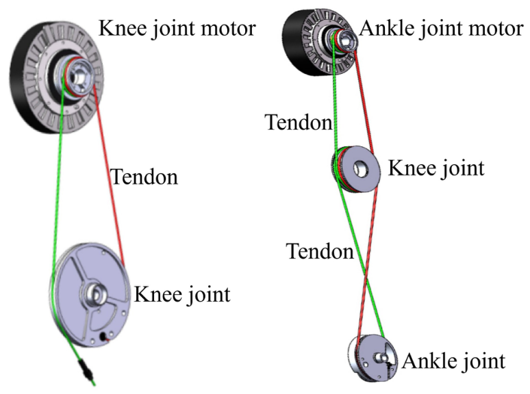
The joint driving method of biped robots directly determines their dynamic characteristics and control complexity. Unlike traditional rigid linkage drives, tendon drives transmit the motor power located at the proximal end of the body to the distal joints, achieving lightweight leg structures and enhanced mobility. However, this driving method also introduces modeling uncertainties and control challenges, becoming a core bottleneck in sim2real transfer. Figure 1 illustrates the differences in the driving methods between the simulation system and the physical robot. Specifically, a direct-drive motor is fixed at the base of the thigh, and its output is transmitted through tendons to the knee joint’s disk to achieve knee flexion and extension. Meanwhile, another motor located at the base of the thigh transmits power through the knee joint’s steering structure to the ankle joint, thereby driving the forward and backward swing of the foot. In simulation modeling, to simplify dynamic calculations and improve simulation efficiency, motors are typically placed directly at each joint, using a joint direct-drive model. Each joint is driven by an independent ideal motor, ignoring non-ideal factors such as tendon elasticity, friction, slack, and transmission delay. However, in the physical system, motors are concentrated at the hip and transmit power remotely through tendons. This fundamental difference leads to significant dynamic discrepancies between the simulation model and the physical system. The complexity of tendon transmission is primarily reflected in the following aspects:

• Elasticity and Stiffness Variation: Tendons are typically made of polymer steel wires, which have certain axial elasticity. Their stiffness is influenced by pre-tension, bending radius, and load, resulting in non-linear spring characteristics in joint torque transmission. During dynamic motion, the elastic deformation of the tendon can cause joint response lag and oscillations, which are difficult to accurately replicate in a rigid joint model.
• Friction and Damping: The contact friction between the tendon and the pulley, as well as the internal damping of the tendon fibers, consumes energy and introduces non-linear damping terms. At low speeds, frictional forces can cause stick-slip effects, affecting the stability of fine control.
• Backlash and Slack: Over long periods of use, tendons may experience plastic elongation or slack, leading to joint backlash and repeatability errors. Time-varying backlash is difficult to model in simulation but significantly impacts the control precision of the physical system.
• Multi-Joint Coupling: Because tendons often use distal transmission designs, the kinematics and dynamics between joints are more coupled. The motion of one joint can affect the tension of another joint via the tendons, which cannot be captured by the simplified joint direct-drive model used in simulation.
• Delay and Bandwidth Limitations: The elasticity and mass distribution of the tendon can result in limited speed of force transmission, causing the joint’s actual response to lag behind the motor commands. High-frequency control signals may be attenuated by the low-pass filtering characteristics of the tendon, thus limiting the system’s controllable bandwidth.

These factors collectively cause a significant degradation in performance when locomotion policies trained in a simulation environment are transferred to the physical robot. The rigid joint movements learned in simulation may oscillate due to tendon elasticity, or fail to precisely follow commands due to friction. Rapid terrain disturbance compensation behaviors may become unstable due to transmission delays. Therefore, narrowing the sim2real gap caused by tendon drives requires algorithms that are robust to unmodeled dynamics, or explicitly consider tendon characteristics during training.

4. Method

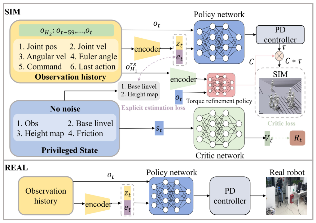
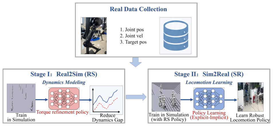
The proposed RSR method consists of two training stages, as illustrated in Figure 2. Each stage adopts an asymmetric actor–critic architecture. In this architecture, the critic network receives privileged information. This privileged information not only includes noise-free proprioceptive observations but also contains additional data crucial for decision-making during training. This additional information is typically difficult to obtain in the real world, such as the full map of the environment, the relative position of the robot to the environment, and auxiliary data from external sensors. Privileged information provides the critic network with a more comprehensive and accurate state representation, allowing it to more effectively evaluate the policy’s value and guide the policy network’s optimization.

The first stage is the Real2Sim (RS) stage, as shown in Figure 3. In this stage, RL is used to model the robot’s time-varying dynamics in simulation. The second stage trains the robot to perform locomotion using RL. Unlike conventional locomotion learning frameworks, in RSR, the torque executed by the robot’s motors is composed of a mixed torque from the first and second stages, as shown in Figure 4. Finally, in the physical deployment stage, the robot executes the torque computed from the joint target positions output by the second-stage policy network.

4.1. Reinforcement Learning-Based Modeling of Proprioceptive Time-Varying Dynamics

Tendon-driven robots exhibit significant time-varying characteristics in their proprioceptive dynamics. Their internal states are typically unobservable, and there are complex coupling relationships between various dynamic parameters. From a system perspective, such actuators involve nonlinear effects such as elastic deformation, damping dissipation, and hysteresis, which make their dynamics exhibit high-dimensional, nonlinear, and time-varying characteristics. In theoretical modeling, accurately characterizing such systems typically requires the introduction of numerous dynamic parameters. However, high-dimensional parameters not only increase modeling complexity but also make the model highly sensitive to real-world data. This results in the model struggling to maintain stability and generalization across different operating conditions. Moreover, due to limited disclosure by manufacturers regarding the actuator’s internal structure and key parameters, parameter identification methods based on analytical modeling are often difficult to implement in practice. In terms of simulation modeling, current mainstream simulation platforms (such as MuJoCo and Isaac Gym) do not support direct modeling of tendon-driven mechanisms. Specifically, parameters such as torque constants, damping, and equivalent rotational inertia in tendon systems dynamically change with the elastic state and joint motion. Existing simulation environments do not provide the necessary functional interfaces to update these time-varying parameters in real time.

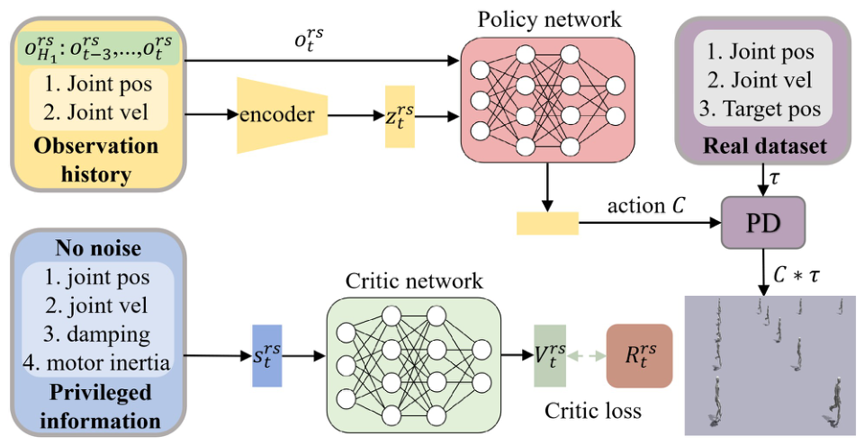
Therefore, we do not explicitly estimate all the parameters of the tendon-driven proprioceptive dynamics. Instead, we treat the difficult-to-characterize dynamic parameters such as elasticity, damping, hysteresis, and joint coupling in the tendon system as deviations from the ideal rigid direct-drive model in the simulation. These deviations are then compensated by a torque fine-tuning strategy learned through training, which enables the modeling of the real-time-varying proprioceptive dynamics. The RS phase, from the perspective of control equivalence, trains a torque fine-tuning strategy to implicitly model the joint torque’s effect on its proprioceptive time-varying dynamics, as shown in Figure 3. In this phase, the historical observation sequence is mapped to a compact latent vector representation through an encoder, which, together with the current observation, serves as input to the policy. During training, the encoder and policy are jointly optimized end-to-end based on the PPO loss, allowing the latent vector to adaptively capture latent factors relevant to optimal control under task-driven conditions. The RS training phase consists of three neural networks: the actor ${\pi }_{rs}\left({\mathit{c}}_t\right|{\mathit{o}}_t^{rs},{\mathit{z}}_t^{rs})$, the critic $V_{rs}$, and the encoder $N_{rs}\left({\mathit{z}}_t\right|{\mathit{o}}_{H_1}^{rs})$. All three networks operate at a frequency of 100 Hz.

The policy network takes the latent variable ${\mathit{z}}_t^{rs}$ generated by the encoder and the current observation ${\mathit{o}}_t^{rs}$ as inputs, and outputs the action ${\mathit{c}}_t$. The input to the encoder is the historical joint information ${\mathit{o}}_{H_1}^{rs}$. The vector ${\mathit{o}}_{H_1}^{rs}$ is an 80-dimensional vector consisting of joint positions and velocities from 4 different time steps, which are directly measured by the robot’s joint sensors. It is defined as

$${\mathit{o}}_t^{rs}={\left[\begin{array}{cc}{\mathit{q}}_t^{rs}& {\dot{\mathit{q}}}_t^{rs}\end{array}\right]}^T$$

(1)

where, ${\mathit{q}}_t^{rs}$ is the joint position, and ${\dot{\mathit{q}}}_t^{rs}$ is the joint velocity.

The policy network takes the current joint position ${\mathit{q}}_t^{rs}$ and velocity ${\dot{\mathit{q}}}_t^{rs}$ as explicit inputs. The theoretical basis for this lies in the fact that the dynamics of biped robots can be described by a system of second-order differential equations. According to classical control theory, for a fully actuated second-order mechanical system, its instantaneous dynamic state is uniquely determined by generalized coordinates and generalized velocities. Therefore, by using ${\mathit{q}}_t^{rs}$ and ${\dot{\mathit{q}}}_t^{rs}$ as inputs to the policy network, we provide the necessary foundational state information for the torque fine-tuning strategy, effectively modeling the complex time-varying dynamics of the tendon-driven system.

The input to the critic network is the privileged information ${\mathit{s}}_t^{rs}$. The vector ${\mathit{s}}_t^{rs}$ consists of the noise-free observation ${\mathit{o}}_t^{rs}$ and some additional information that is difficult to obtain in reality. It is defined as:

$${\mathit{s}}_t^{rs}={\left[\begin{array}{ccc}{\mathit{o}}_t^{rs}& {\mathit{d}}_t^{rs}& {\mathit{m}}_t^{rs}\end{array}\right]}^T$$

(2)

where, ${\mathit{d}}_t^{rs}$ is the joint damping, and ${\mathit{m}}_t^{rs}$ is the motor’s rotational inertia.

The policy network is updated using the PPO algorithm. This method optimizes the clipped objective function of the policy, combined with mini-batch stochastic gradient descent, to approximate the maximization of the expected return. The loss function is defined as:

$$\begin{array}{cc}\hfill {\mathcal{L}}_{\pi }=min& {\displaystyle (\frac{{\pi }_{\theta }\left({\mathit{a}}_t\right|{\mathit{s}}_t)}{{\pi }_{{\theta }_b}\left({\mathit{a}}_t\right|{\mathit{s}}_t)}}{A}^{{\pi }_{{\theta }_b}}({\mathit{s}}_t,{\mathit{a}}_t),\hfill \\ \hfill & \mathrm{clip}\left({\displaystyle \frac{{\pi }_{\theta }\left({\mathit{a}}_t\right|{\mathit{s}}_t)}{{\pi }_{{\theta }_b}\left({\mathit{a}}_t\right|{\mathit{s}}_t)}},1-ϵ,1+ϵ\right)A^{{\pi }_{{\theta }_b}}({\mathit{s}}_t,{\mathit{a}}_t))\hfill \end{array}$$

(3)

During the policy update process, ${\pi }_{\theta }$ represents the current target policy to be optimized, while ${\pi }_{{\theta }_b}$ is the behavior policy from the previous iteration. To prevent large deviations in the policy, the PPO algorithm introduces a clipping mechanism, where $ϵ$ is the clipping hyperparameter used to limit the fluctuation range of the ratio between the new and old policies. To evaluate the quality of action ${\mathit{a}}_t$ relative to state ${\mathit{s}}_t$ under the old policy ${\pi }_{{\theta }_b}$, PPO introduces the advantage function $A^{{\pi }_{{\theta }_b}}({\mathit{s}}_t,{\mathit{a}}_t)$. This advantage function is estimated by the value function $V_{\varphi }\left({\mathit{s}}_{\mathit{t}}\right)$, which is trained by fitting the true returns to reduce the prediction error of the returns. The optimization objective of the value function is:

$${\mathcal{L}}_v={\left(V_{\varphi }\left({\mathit{s}}_t\right)-{\widehat{R}}_t\right)}^2$$

(4)

The training hyperparameters for the RS stage are shown in

Table 2. Training hyperparameter settings for dynamics modeling.

Parameter	Value
Number of Environments	4096
Learning Rate	5 × 10−4
Discount Factor	0.99
GAE Coefficient	0.95
Number of Batches	5
Gradient Clipping	1
Clipping Range	0.2
Entropy Coefficient	0.002
Policy Hidden Layers	[256, 128]
Critic Hidden Layers	[256, 128]
Encoder	[256, 128]
$H_1$	4

. The settings for these hyperparameters aim to improve the efficiency of large-scale parallel training and the stability of policy learning. During training, 4096 parallel environments are used to fully utilize GPU resources, thereby improving data sampling efficiency and accelerating policy convergence.

We also constructed a high-quality real-world dataset. During the data collection process, the robot’s body height was kept constant, and the foot trajectory was parametrically excited. Specifically, a sine function was used to plan the foot trajectory, and inverse kinematics were employed to map the desired foot position to the target joint positions. During execution, the foot continuously makes contact with and detaches from the ground, allowing the collected data to cover key dynamic patterns similar to those encountered in locomotion control. To improve the data’s coverage and diversity, the amplitude of the sine function varied within a range of 5–20 cm, while the frequency was systematically adjusted within a range of 1–25 Hz to ensure sufficient excitation of the trajectory in both time and frequency domains, avoiding unnatural oscillations during training. For joint control, a low stiffness PD controller was used for position tracking. Except for the ankle joint, whose PD controller parameters were set to 30 and 1, respectively, all other joints were set to 100 and 2, respectively. During the swing phase, key state information such as target joint positions, actual joint positions, and joint velocities were recorded for subsequent model training. The real-world robot’s body dynamics were then transferred to the simulation environment using an RL method. Specifically, joint target positions, joint positions, and joint velocity sequences were randomly sampled from the real robot’s collected data. The first time step of each sampled sequence’s joint position and velocity were used to initialize the simulation robot’s state. The duration of each data sequence was 1 s. The simulation robot then tracked the corresponding joint target positions from the second time step onward. The RS training round was terminated when the simulation time reached 24 s. Finally, a policy network was trained to adjust the torque values of the joints, ensuring that the joint motion behavior in the simulation environment matched the dynamic response observed in the real robot. The policy obtained through this RS training process was able to effectively replicate the real robot’s system dynamics.

Since the data in the real-world dataset contains noise, we introduced domain randomization in the simulation environment. The randomization ranges for each parameter are shown in

Table 3. Domain randomization settings in RS stage training.

Parameter	Unit	Range
Joint Position	rad	$\mathcal{U}(-0.05,0.05)$
Joint Velocity	rad/s	$\mathcal{U}(-2,2)$

. $\mathcal{U}(a,b)$ denotes a uniform distribution, with noise uniformly distributed within the range $[a,b]$. Furthermore, on the real robot, it is usually difficult to directly obtain joint velocities from sensors. In practice, joint velocity is often estimated by numerically differentiating the joint position signals. However, this process can amplify the measurement noise from the joint position sensors, resulting in poor quality of the velocity signal. To reflect this realistic situation, strong additive noise $\mathcal{U}(-2,2)$ rad/s was introduced to the joint velocity observation during training to simulate the uncertainty in real measurements.

In the simulation, to model the dynamic changes of the tendon-driven biped robot, the robot executes a PD controller at 500 Hz. The joint target positions ${\mathit{q}}_{\mathrm{tar}}^{rs}$ correspond to the trajectories recorded during the data collection phase. The control method is:

$$\mathit{\tau }={\mathit{c}}_t·\left({\mathit{k}}_p({\mathit{q}}_{tar}^{rs}-{\mathit{q}}^{rs})-{\mathit{k}}_d{\dot{\mathit{q}}}^{rs}\right)$$

(5)

where, ${\mathit{k}}_p$ and ${\mathit{k}}_d$ are consistent with the real robot controller.

To ensure that the simulation controller’s response under the same trajectory is consistent with the real robot while maintaining smooth outputs, the reward function in the RS stage is:

$$\mathit{r}=exp\left(-100\parallel {\mathit{q}}_{real}-{\mathit{q}}_{sim}{\parallel }^2\right)-0.01{\parallel {\mathit{c}}_t-{\mathit{c}}_{t-1}\parallel }^2$$

(6)

where, ${\mathit{q}}_{real}$ is the recorded joint position of the real robot, and ${\mathit{q}}_{sim}$ is the joint position from the simulation.

It is worth noting that the output ${\mathit{c}}_t$ of the policy network is subjected to a clamping process, limiting it to the range $[0.8,1.2]$. This constraint is used to limit the torque adjustment magnitude, preventing the policy from producing excessively large or small corrections, thus avoiding the robot from violating physical constraints or causing instability during the locomotion training process in the second stage. By keeping the action space within a reasonable range, the stability of the policy optimization process can be effectively enhanced, and the interference of extreme actions on training can be reduced. On the other hand, when the system enters a state distribution not covered by the training dataset, the torque fine-tuning policy may produce outputs that deviate from the normal range. The clamping process in this case acts as a conservative constraint mechanism, ensuring that the policy output remains within an acceptable range, thereby preventing abnormal control signals from damaging the system. At the same time, since the output can still vary within this range, such constrained disturbances manifest, to some extent, as implicit randomization of the executed torque during the sim2real process, helping to alleviate the policy’s over-reliance on the training data distribution, thus improving its robustness and generalization ability in unknown environments.

4.2. An Explicit–Implicit Learning Approach for Locomotion Training

In the first stage, the RS method is used to model the time-varying dynamics of the body. The trained torque fine-tuning policy adjusts the executed torque of the joints in the simulation according to the robot’s current state. We deploy the trained torque fine-tuning policy into the locomotion training RL framework. In the second stage, the network parameters of the torque fine-tuning policy are fixed and do not participate in gradient updates. They are only used to reduce the gap between the simulation robot’s body dynamics and the real robot, as shown in Figure 4.

In the locomotion training framework based on explicit–implicit learning, the policy network receives the explicit–implicit information encoded from historical body observations and the current observation ${\mathit{o}}_t$ as input, while the critic network receives the complete privileged information ${\mathit{s}}_t$. ${\mathit{o}}_t$ is defined as

$${\mathit{o}}_t={\left[\begin{array}{ccccc}\mathit{cmd}& {\mathit{q}}_t& {\dot{\mathit{q}}}_t& \mathbf{\Phi }& \mathit{\omega }\end{array}\right]}^T$$

(7)

where, $\mathit{cmd}$ represents the desired motion command and gait phase signal. ${\mathit{q}}_t$ and ${\dot{\mathit{q}}}_t$ represent the joint position and joint velocity, respectively, while $\mathbf{\Phi }$ and $\mathit{\omega }$ represent the body posture and angular velocity. ${\mathit{q}}_t$ and ${\dot{\mathit{q}}}_t$ can be obtained from the joint encoders, while $\mathbf{\Phi }$ and $\mathit{\omega }$ can be obtained from the IMU. The $\mathit{cmd}$ is provided by the higher-level control module.

The policy relies solely on historical observation information ${\mathit{o}}_{H_2}$ and does not use any privileged information, ensuring deployability on the real robot. The input to the critic network is the privileged information ${\mathit{s}}_t$, defined as

$${\mathit{s}}_t={\left[\begin{array}{cccc}{\mathit{o}}_t& {\mathit{v}}_t& {\mathit{h}}_t^{\mathrm{feet}}& {\mu }_t\end{array}\right]}^T$$

(8)

where ${\mathit{v}}_t$ represents the noise-free body linear velocity, ${\mathit{h}}_t^{\mathrm{feet}}$ is the terrain elevation map under the feet, and ${\mu }_t$ is the ground friction coefficient. It is important to emphasize that the ${\mathit{o}}_t$ received by the critic network does not contain any sensor noise. This design helps reduce the variance in value function estimation and improves training stability. The privileged information input to the critic network in the second stage is more comprehensive compared to the first stage. This difference arises from the different learning objectives of the two stages.

In the first stage of modeling the time-varying body dynamics, the critic’s input mainly consists of the system’s body dynamics parameters. In the second stage of locomotion training, the critic network requires not only the dynamics parameters but also environment features related to the locomotion task, including body linear velocity, terrain elevation map under the feet, and other information.

The policy network is represented as ${\pi }_{\theta }\left({\mathit{a}}_t\right|{\mathit{e}}_t,{\mathit{z}}_t,{\mathit{o}}_t)$. In the sim2real transfer framework, an explicit–implicit learning network is introduced, which consists of an encoder $N_{sr}({\mathit{e}}_t,{\mathit{z}}_t|{\mathit{o}}_{H_2})$ at its core, as shown in Figure 4. The goal of this network is to extract explicit information ${\mathit{e}}_t$ and implicit representations ${\mathit{z}}_t$ from the historical observation sequence ${\mathit{o}}_{H_2}$. This network aims to extract two complementary representations from the historical observation sequence ${\mathit{o}}_{H_2}$: explicit information ${\mathit{e}}_t$ and implicit representations ${\mathit{z}}_t$. Explicit information is used to estimate key state quantities that are difficult to directly obtain in the real-world environment for locomotion tasks; implicit representations focus on extracting task-specific optimal representations related to control decisions, thus providing more effective feature support for policy learning. The explicit information ${\mathit{e}}_t$ consists of two parts: ${\tilde{\mathit{v}}}_t$, the explicitly estimated body linear velocity, and ${\tilde{\mathit{h}}}_t^{\mathrm{feet}}$, the explicitly estimated terrain elevation map under the feet. These explicit variables have corresponding real values in the simulation environment and can be trained through a loss function to guide the encoder to learn state representations with clear physical meaning. In contrast, the implicit representation ${\mathit{z}}_t$ does not correspond to a specific physical quantity. It is primarily used to capture latent representations in the historical observations that are task-related but difficult to explicitly model (such as unmodeled dynamics, contact uncertainty, etc.), thereby improving the policy’s adaptability to various complex environments.

The loss of the explicit estimation is defined as

$${\mathcal{L}}_{\mathrm{ed}}=\parallel {\mathit{v}}_t-{\tilde{\mathit{v}}}_t{\parallel }_2+{\parallel {\mathit{h}}_t^{\mathrm{feet}}-{\tilde{\mathit{h}}}_t^{\mathrm{feet}}\parallel }_2$$

(9)

where, ${\mathit{v}}_t$ and ${\mathit{h}}_t^{\mathrm{feet}}$ denote the ground-truth linear velocity and the terrain height map under the feet, respectively.

During the locomotion control training phase, the policy network, critic network, and encoder are optimized jointly in an end-to-end manner. The overall loss function is defined as

$${\mathcal{L}}_{\mathrm{sr}}={\mathcal{L}}_{\mathrm{ed}}+{\mathcal{L}}_{\pi }+{\mathcal{L}}_v$$

(10)

where, ${\mathcal{L}}_{\pi }$ and ${\mathcal{L}}_v$ denote the policy loss and critic loss, respectively. Through this joint optimization mechanism, the policy network, critic network, and encoder can collaborate efficiently, thereby improving the stability and convergence speed of training. The encoder not only learns implicit representations but also provides auxiliary information to the policy through explicit estimation, helping generate more precise control commands. Moreover, joint optimization accelerates the training process and improves sample efficiency. The hybrid explicit–implicit learning approach combines the advantages of explicit estimation and implicit representation, enhancing the stability of the policy and its adaptability to tasks.

4.3. Locomotion Training Environment Design

To achieve stable bipedal locomotion control, we designed a RL-based training environment, which mainly includes the design of the action space, reward function, and domain randomization. The core objective of this environment is to provide a reliable training foundation for subsequent deployment on real robots, while ensuring control stability.

The action ${\mathit{a}}_t$ is a 10-dimensional vector representing the residual of the default joint positions ${\mathit{q}}_d$. Actions generated by the policy are updated at a frequency of 100 Hz and passed to the joint PD controller. The joint PD controller then operates at a frequency of 500 Hz. It converts the actions into desired torque commands using the following formula:

$$\mathit{\tau }={\mathit{c}}_t·\left({\mathit{k}}_p({\mathit{a}}_t+{\mathit{q}}_d-\mathit{q})-{\mathit{k}}_d\dot{\mathit{q}}\right)$$

(11)

where, ${\mathit{q}}_d$ denotes the default joint positions.

The reward function is designed to guide the robot in tracking velocity commands while maintaining posture stability, as detailed in

Table 4. Reward function components.

Reward Term	Formula	Weight
Linear Velocity Tracking	$exp\left(-4\parallel {\mathit{v}}_{xy}^{\mathrm{cmd}}-{\mathit{v}}_{xy}{\parallel }^2\right)$	1
Angular Velocity Tracking	$exp\left(-4{({\omega }_z^{\mathrm{cmd}}-{\omega }_z)}^2\right)$	1
Angular Velocity Penalty	$\parallel {\mathit{\omega }}_{xy}{\parallel }^2$	−0.1
Body Posture Penalty	$\parallel {\mathit{g}}_{xy}{\parallel }^2$	−2
COM Height Penalty	${(h-h_{\mathrm{des}})}^2$	−1
Joint Power Penalty	$\parallel \mathit{\tau }\dot{\mathit{q}}{\parallel }^2$	$-1\times {10}^{-3}$
Joint Acceleration Penalty	$\parallel \ddot{\mathit{q}}{\parallel }^2$	$-2.5\times {10}^{-7}$
Action Rate Penalty	$\parallel {\mathit{a}}_t-{\mathit{a}}_{t-1}{\parallel }^2$	−0.01
Stance-Phase Penalty	$r_{\mathrm{fc}}$	−1
Swing-Phase Penalty	$r_{\mathrm{fv}}$	−1
Body Collision Penalty	$n_{\mathrm{collision}}$	−1

. The linear and angular velocity tracking terms provide the primary driving signals, encouraging the robot to execute locomotion tasks according to the desired commands. The angular velocity penalty suppresses rotations of the torso in the horizontal plane, reducing the impact of excessive spinning on balance. The body posture penalty constrains the torso’s tilt, maintaining overall postural stability. The center-of-mass height penalty guides the robot to maintain the desired height, preventing abnormal gait patterns. The joint power penalty limits joint energy consumption, discouraging high-power actions and promoting smoother gait. The joint acceleration penalty suppresses abrupt changes in joint accelerations to prevent sudden motions. The action rate penalty constrains the magnitude of action changes between consecutive time steps, improving the continuity of control signals. The stance-phase and swing-phase penalties regulate periodic foot behavior, ensuring gait periodicity and stability. The body collision penalty encourages the robot to avoid contact with environmental obstacles, thereby enhancing walking safety.

The symbols in Table 4 are defined as follows: ${\mathit{v}}_{xy}^{\mathrm{cmd}}$ and ${\mathit{v}}_{xy}$ denote the commanded and actual linear velocities, respectively; ${\omega }_z^{\mathrm{cmd}}$ and ${\omega }_z$ are the commanded and actual angular velocities about the vertical (z) axis. ${\mathit{g}}_{xy}$ is the projection of the gravity vector onto the horizontal plane of the body frame, used to measure torso tilt; ${\mathit{\omega }}_{xy}$ represents the angular velocity vector of the torso around the horizontal axes (pitch and roll directions). h and $h_{\mathrm{des}}$ denote the actual and desired base heights of the robot, respectively. In the dynamics terms, $\mathit{\tau }$, $\dot{\mathit{q}}$, and $\ddot{\mathit{q}}$ represent the joint torques, joint velocities, and joint accelerations; $\parallel \mathit{\tau }\dot{\mathit{q}}\parallel$ characterizes joint power consumption. Regarding control inputs, ${\mathit{a}}_t$ and ${\mathit{a}}_{t-1}$ denote the current and previous action commands, used to constrain action smoothness. $n_{\mathrm{collision}}$ counts the number of leg collision events within the current step.

$r_{\mathrm{fc}}$ and $r_{\mathrm{fv}}$ are penalties based on foot contact states and foot-end velocities, respectively. The reasonableness of foot-end motion within a gait cycle directly affects locomotion stability and terrain adaptability. To this end, a binary foot contact indicator $I_i\left(t\right)$ is introduced: $I_i\left(t\right)=0$ when the i-th leg is in the stance phase, and $I_i\left(t\right)=1$ when it is in the swing phase. During the swing phase, unintended contact between the foot and the ground should be avoided; therefore, the foot contact force is penalized as follows:

$$r_{\mathrm{fc}}=\sum _i{I}_i\left(t\right)[1-exp\left(-{\displaystyle \frac{\parallel {\mathit{f}}_{\mathrm{foot},i}{\parallel }^2}{50}}\right)],$$

(12)

where, ${\mathit{f}}_{\mathrm{foot},i}$ denotes the foot contact force vector. This penalty encourages the swing leg to lift actively, preventing contact with the ground.

During the stance phase, the foot should remain relatively stationary to provide stable support; therefore, the horizontal velocity of the foot is penalized as follows:

$$r_{\mathrm{fv}}=\sum _i[1-I_i\left(t\right)][1-exp\left(-4\parallel {\mathit{v}}_{xy}^{\mathrm{foot},i}{\parallel }^2\right)],$$

(13)

where, ${\mathit{v}}_{xy}^{\mathrm{foot},i}$ denotes the velocity vector of the foot in the horizontal plane.

The simulation episode is limited to 24 s. Under normal circumstances, the simulation continues until the maximum time step is reached. If any termination condition is triggered during execution, the current episode is terminated early. This prevents the collection of invalid data under unstable conditions and preserves learning efficiency. The termination conditions are defined as follows:

• When the absolute value of the torso roll or pitch angle exceeds 0.785 rad.
• When the height of the torso’s center of mass falls below 0.3 m.

During task execution, the target velocity commands are not constant but are randomly resampled at intervals of 2–6 s. The command types include five typical behaviors: [standing in place, forward/backward walking, lateral walking, in-place turning, omnidirectional walking]. The corresponding linear and angular velocity command spaces are set as: $v_x^{\mathrm{cmd}}\in [-0.5,2.8]$ m/s, $v_y^{\mathrm{cmd}}\in [-1,1]$ m/s, and ${\omega }_z^{\mathrm{cmd}}\in [-1,1]$ rad/s, ensuring coverage of diverse walking requirements.

To simulate real sensor noise and dynamics uncertainty, and to reduce the distribution gap between simulation and the real system, domain randomization is introduced in the simulation environment. Unlike the domain randomization in Table 3, the second-stage locomotion training applies random noise perturbations at the observation, dynamics, and control levels, exposing the policy to diverse system uncertainties during training and thereby enhancing its robustness and generalization capability on real robots. Observation-level randomization includes joint position noise, joint velocity noise, Euler angle noise, and angular velocity noise, simulating sensor measurement noise and uncertainties from numerical differentiation. Dynamics-level randomization includes center-of-mass offsets, payload mass variations, and friction coefficient perturbations, modeling changes in mass distribution, external load disturbances, and contact environment uncertainties in real systems. Control-level randomization perturbs the ${\mathit{k}}_p$ and ${\mathit{k}}_d$ gains to simulate calibration errors of the actual controller and variations in actuator responses. The specific perturbation ranges for each randomization parameter are listed in

Table 5. Domain randomization settings for locomotion training.

Parameter	Unit	Range
Joint Position Noise	rad	$\mathcal{U}(-0.05,0.05)$
Joint Velocity Noise	rad/s	$\mathcal{U}(-2,2)$
Euler Angle Noise	rad	$\mathcal{U}(-0.05,0.05)$
Angular Velocity Noise	rad/s	$\mathcal{U}(-0.5,0.5)$
Center-of-Mass Offset	cm	$\mathcal{U}(-0.075,0.075)$
Payload Mass	kg	$\mathcal{U}(-5,5)$
Friction Coefficient	-	$\mathcal{U}(0.3,2)$
${\mathit{k}}_p,{\mathit{k}}_d$ Gain Noise	-	$\mathcal{U}(0.85,1.15)$

, where $\mathcal{U}(a,b)$ denotes a uniform distribution over the interval $[a,b]$.

The policy is trained using the PPO algorithm, with hyperparameter settings listed in

Table 6. Training hyperparameter settings.

Parameter	Value
Number of Environments	4096
Learning Rate	Adaptive
Discount Factor	0.99
GAE Coefficient	0.95
Number of Batches	5
Gradient Clipping	1
Clipping Range	0.2
Entropy Coefficient	0.01
Policy Hidden Layers	[512, 256, 128]
Critic Hidden Layers	[512, 256, 128]
Encoder	[512, 256, 128]
$H_1$, $H_2$	4, 60

. In this section, the length of the historical observation window $H_2$ is set to 60 to fully capture the dynamic evolution characteristics of the robot during walking. Since locomotion training in the second stage is significantly more challenging than in the first stage, different learning rates and entropy coefficients are employed. The first-stage tasks are relatively simple, so a fixed learning rate and a smaller entropy coefficient are used to ensure training stability and convergence speed. In contrast, the second-stage tasks are considerably more complex. Therefore, an adaptive learning rate strategy is adopted to dynamically adjust step sizes during training, avoiding local optima. The entropy coefficient is also increased to 0.01 to encourage higher exploration in complex locomotion tasks, preventing premature convergence to suboptimal policies. Moreover, the hidden layer dimensions of the policy and critic networks are deepened to enhance the model’s representation capability for high-dimensional state and action spaces. These adjustments collectively improve the learning efficiency and control performance of the model in complex locomotion tasks.

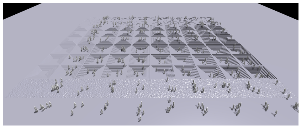
During training, a terrain curriculum strategy is introduced to dynamically adjust environment difficulty and facilitate progressive adaptation of the policy to unstructured terrains, as illustrated in Figure 5, where the terrain from left to right represents increasing levels of difficulty. Specifically, after each environment reset, the system first computes the planar distance between the robot’s root position and the starting point of the terrain, using this distance as a measure of performance on the current terrain. If the robot walks more than half of the terrain length, its performance is considered satisfactory, and the terrain level is increased, allowing it to train on a more difficult terrain. For robots that do not meet the distance requirement, the system further evaluates performance using the cumulative linear velocity reward: if the average linear velocity falls below a predefined threshold, the terrain level is decreased, placing the robot on an easier terrain to prevent instability or abnormal behavior at excessive difficulty. After the terrain level is updated, the robot’s environment start point is adjusted accordingly to align with the new terrain configuration. To maintain diversity and challenge, robots that reach the maximum terrain level are randomly assigned a terrain not exceeding the highest level, preventing the policy from overfitting to a specific terrain pattern while preserving exploration. This curriculum mechanism ensures that each robot can adaptively progress to an appropriate terrain difficulty according to its capability, enabling stable policy execution while gradually improving robustness across diverse, unstructured environments, thereby enhancing the transfer of simulation-trained policies to complex real-world scenarios.

5. Experimental Results

To evaluate the sim2real transfer performance of RSR and its adaptability to complex terrains, extensive locomotion experiments were conducted in both simulation and on a real robot platform. The experiments were conducted on the tendon-driven bipedal robot X02 developed by Shanghai DroidUp Co., Ltd. The robot has a height of approximately 1.70 m and a total weight of approximately 32 kg. Detailed hardware specifications of the platform can be found in [22]. We controlled only the 10 degrees of freedom of the lower body, and the policy network runs at 100 Hz on the RK3588. By systematically testing under a variety of challenging terrain conditions, the locomotion control performance of different methods during sim2real transfer was comprehensively assessed. Three representative methods were selected for ablation and comparison with RSR. All four algorithms were trained using the same locomotion training environment. These algorithms are:

• Rapid Motor Adaptation (RMA) [14]: A two-stage teacher–student framework. In this baseline, the teacher policy is first trained in simulation using privileged information, and then distilled to a student network that relies solely on proprioceptive observations via imitation learning.
• Implicit World Representation (IWM): Purely implicit method (RSR w/o Explicit and RS). In this ablation, explicit estimation information and the torque refinement network are removed.
• Explicit–Implicit World Representation (EIWM): Explicit–implicit learning method (RSR w/o RS). In this ablation, the torque refinement policy network is removed from the locomotion training framework.
• RSR: Our method.

5.1. Simulation Ablation Experiments

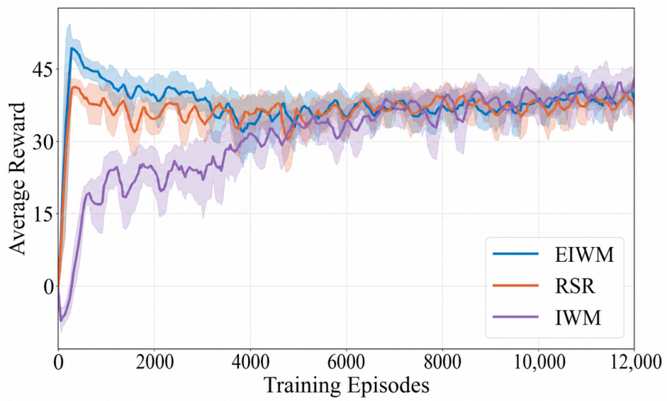
We conducted a comparative analysis of the EIWM, IWM, and RSR methods in the simulation environment. Since the RMA method employs a two-stage training framework, its advantage primarily lies in cross-stage transfer capability and is therefore not included in this comparison. By comparing the three aforementioned methods, we can systematically analyze the impact of explicit–implicit learning on policy training efficiency and control performance. It should be noted that the primary purpose of RSR in the simulation environment is to verify whether the torque refinement policy affects locomotion control performance, with its advantages becoming apparent during deployment on the real system. The reward curves of the three methods during training are shown in Figure 6.

As shown in

Table 7. Convergence Analysis of Different Methods.

Method	Average Reward	Episodes to 80% Final Reward
EIWM	0.9532	192
IWM	0.8268	1770
RSR	0.9768	192

, both EIWM and RSR reach a high-reward region within approximately 200 episodes, with a convergence speed significantly faster than that of IWM. This result indicates that, compared to relying solely on implicit representations, incorporating explicit estimation information can substantially improve sample efficiency during policy learning, thereby accelerating convergence. In terms of policy performance, the average rewards of EIWM and RSR are 35.67 and 35.83, respectively, both close to each other and significantly higher than IWM’s 23.33. This demonstrates that explicit–implicit learning can effectively enhance policy performance, and introducing the torque refinement policy in the locomotion training framework does not negatively affect the locomotion policy’s performance. Regarding training stability, the reward standard deviations of EIWM and RSR are 3.40 and 3.36, respectively, both notably lower than IWM’s 4.55. This shows that the explicit–implicit learning approach effectively reduces fluctuations during training, improving stability. Since EIWM and RSR perform similarly on this metric, the stability improvement mainly arises from the inclusion of explicit estimation information rather than the torque refinement policy in the RS stage. Overall, the hybrid explicit–implicit method outperforms the purely implicit method in convergence speed, policy performance, and training stability. On this basis, introducing the torque refinement policy network does not degrade policy performance, validating the design rationale of the RS stage.

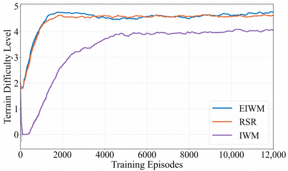
The terrain difficulty levels during training for the three algorithms are shown in Figure 7. The average terrain difficulty level for EIWM is 4.58, and for RSR it is 4.56, both higher than IWM’s 3.68. This result indicates that, compared to methods relying solely on implicit representations, incorporating explicit estimation information allows the policy to access clearer footstep elevation map information. Consequently, the policy can more easily tackle higher-difficulty terrains during training and exhibit better environmental adaptability. This suggests that the explicit estimates of linear velocity and local terrain height under the feet provide the policy with more direct motion and geometric priors, enhancing the usability of state information and improving learning efficiency in complex environments.

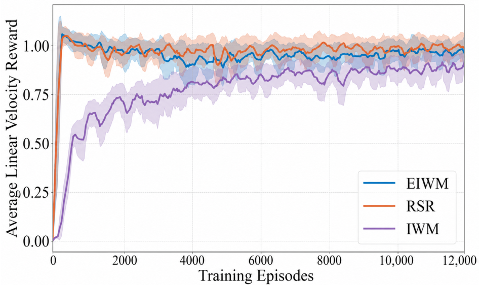
In terms of linear velocity-tracking performance, EIWM and RSR demonstrate significant advantages over the IWM method, as shown in Figure 8. The overall average reward for EIWM is 0.95, for RSR it is 0.97, whereas IWM achieves only 0.82. The primary reason for this difference lies in the way each method estimates velocity information: IWM relies entirely on implicit representations, which introduces uncertainty in expressing velocity-related states and slows down the learning process. In contrast, EIWM and RSR explicitly estimate linear velocity and feed it directly into the policy network, enabling more accurate tracking of velocity commands.

The overall comparison results are shown in

Table 8. Performance metrics of the three algorithms during training.

Method	Average Reward	Average Terrain Level	Average Linear Velocity Reward
IWM	23.33	3.68	0.82
EIWM	35.67	4.58	0.95
RSR	35.83	4.56	0.97

. The three methods exhibit a consistent ranking across all three evaluation metrics: EIWM and RSR perform similarly overall and are consistently better than IWM. This demonstrates that the explicit–implicit learning approach can significantly enhance locomotion training performance. The overall performance of RSR in the simulation environment is essentially equivalent to that of EIWM. The main purpose of comparing RSR in the simulation experiments is to verify whether the introduced torque refinement policy adversely affects policy performance. The results also indicate that the torque refinement policy does not compromise the locomotion control training performance in simulation.

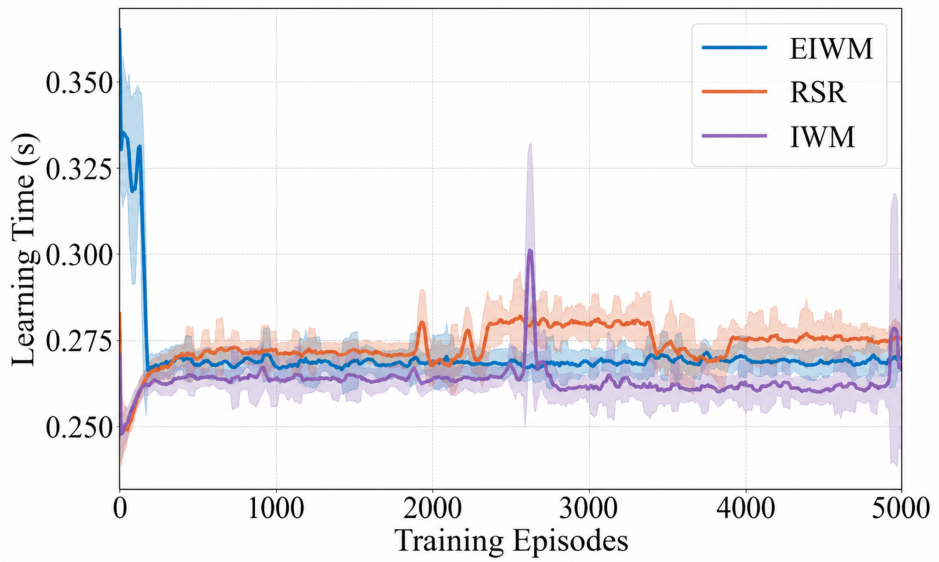
To analyze the computational cost of different methods, we measured the real-time learning time of EIWM, RSR, and IWM during training, as shown in Figure 9. The average learning times of EIWM, RSR, and IWM are 0.2790 s, 0.2760 s, and 0.2738 s, respectively. The differences are relatively small, indicating that the proposed explicit–implicit learning framework and the RS-stage torque refinement strategy do not introduce significant additional computational overhead. Combined with the experimental results presented above, it can be observed that RSR significantly improves velocity-tracking performance, terrain adaptability, and sim2real transfer capability while maintaining a computational cost comparable to the baseline methods. These results demonstrate that the proposed method achieves a favorable balance between performance improvement and computational cost. The performance gains are not obtained through substantially increased computational resources, but rather through more effective state representations and time-varying dynamics modeling.

5.2. Real-World Ablation and Comparison Experiments

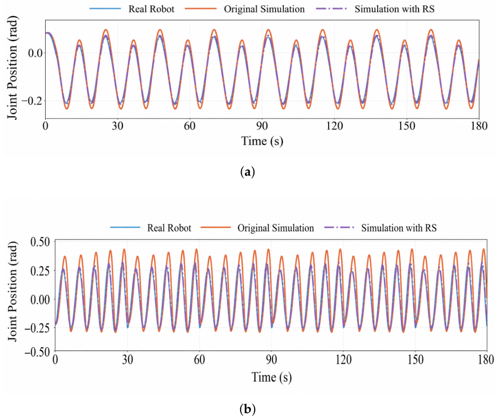
To verify whether the torque refinement policy network can reduce the proprioceptive time-varying dynamics gap in sim2real transfer, we simultaneously executed two planned sets of hip joint target position trajectories on the real robot and in two simulation environments. One simulation environment incorporates the RS-stage torque refinement policy, while the other is the original simulation environment without the torque refinement policy. Neither set of trajectories was included in the RS-stage training dataset, and the trajectories have different motion speeds. After executing the same joint target position commands, the actual joint position trajectories of all three cases were recorded and compared, as shown in Figure 10.

Figure 10a and Figure 10b present the comparison of dynamic responses of the hip joint under low-speed and high-speed motion conditions, respectively. The experimental results indicate that the simulation environment incorporating the torque refinement strategy exhibits significantly higher consistency with the real robot in terms of hip-level proprioceptive dynamics.

Table 9. Joint Tracking RMSE under Low-Speed and High-Speed Motions.

Method	Joint	Low-Speed Motion (rad)	High-Speed Motion (rad)
Original Simulation	Hip	0.0356	0.1590
	Knee	0.0483	0.1985
	Ankle	0.0627	0.2412
Simulation with RS	Hip	0.0148	0.0375
	Knee	0.0219	0.0586
	Ankle	0.0294	0.0743

provides the quantitative comparison of RMSE for the hip, knee, and ankle joints under different motion speeds. Under low-speed motion, the RS method reduces the hip joint RMSE from 0.0356 rad to 0.0148 rad, while the knee and ankle joints are reduced to 0.0219 rad and 0.0294 rad, respectively. Under high-speed motion, the hip joint RMSE decreases from 0.1590 rad to 0.0375 rad, whereas the knee and ankle joints are reduced to 0.0586 rad and 0.0743 rad, respectively. These results indicate that the torque refinement policy effectively enhances the simulation system’s ability to model the time-varying dynamics of the robot during high-speed motion, thereby substantially reducing the sim2real gap. In contrast, the original simulation environment without the refinement strategy exhibits noticeable trajectory deviations under the same conditions, further validating the effectiveness of the torque refinement network in minimizing proprioceptive dynamics discrepancies.

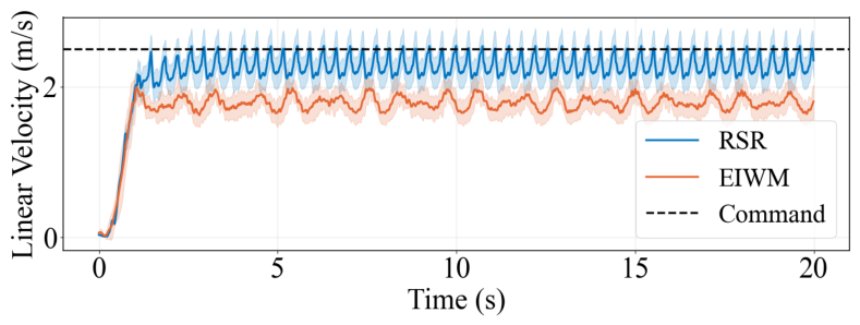
To evaluate the velocity command-tracking performance of different methods in the real world, the robot was commanded to walk at forward speeds of 0.6 m/s, 1.5 m/s, 2.0 m/s, and 2.5 m/s, with each speed maintained for 20 s. For each method and each speed condition, five independent trials were conducted, and the average walking distance was recorded. The results are summarized in

Table 10. Walking distance of the robot in 20 s under four forward velocity commands.

Method	0.6 m/s	1.5 m/s	2.0 m/s	2.5 m/s
RMA	10.5 m	26.8 m	34.5 m	32.1 m
IWM	11.1 m	27.9 m	36.2 m	34.3 m
EIWM	11.5 m	28.6 m	37.5 m	36.8 m
RSR	11.8 m	29.1 m	38.4 m	48.2 m

. The results in Table 10 indicate that, compared to the RMA method, IWM effectively reduces velocity tracking errors through the use of history-based implicit representations, thereby improving the policy’s responsiveness. Building on this, EIWM achieves higher tracking accuracy under all speed conditions by explicitly estimating linear velocity, demonstrating that explicit state estimation can further enhance control performance. RSR, which additionally models the time-varying dynamics of the tendon-driven system on top of EIWM, achieves the best performance across all speed conditions. At the highest speed of 2.5 m/s, RSR achieved an average tracking velocity of 2.41 m/s with a variance of 0.00416, whereas EIWM achieved an average tracking velocity of 1.84 m/s with a variance of 0.0102. In contrast, the tracking accuracy of the other methods degraded significantly, while RSR was still able to stably track the target velocity. Experimental results show that at a maximum speed of 2.5 m/s, the EIWM method with explicit estimation improves the linear velocity tracking accuracy by 15.9% compared to the baseline IWM. Furthermore, the RSR method, which further introduces a torque fine-tuning strategy based on EIWM, achieves an 86.4% improvement in accuracy over EIWM.

From a mechanistic perspective, explicitly estimating the body linear velocity provides the policy network with motion-state information that has clear physical meaning, thereby reducing its reliance on learning velocity-related features solely through implicit representations and improving both velocity tracking accuracy and training efficiency. The study by Li et al. [23] likewise demonstrated that explicitly incorporating linear velocity information can significantly enhance a robot’s ability to track commanded velocities. Furthermore, tendon-driven systems inherently exhibit complex time-varying dynamics, including elastic deformation, transmission delays, friction losses, and multi-joint coupling effects. These factors introduce substantial dynamic discrepancies between simulation environments and real robots [13,24]. The proposed torque refinement policy compensates for these difficult-to-model nonlinear dynamic effects through learning, enabling the simulated robot to more accurately reproduce the dynamic responses of the physical robot. Consequently, under high-speed locomotion conditions, RSR can effectively reduce the sim2real dynamics gap, resulting in improved velocity tracking accuracy and locomotion stability.

When the commanded speed is set to 2.5 m/s, Figure 11 shows the average velocity tracking curves over five independent trials along with their 95% confidence intervals. It can be observed that the RSR method achieves an average tracking velocity of 2.41 m/s, consistently remaining near the commanded speed, with a narrow confidence interval, indicating good stability and repeatability. In contrast, the EIWM method achieves an average tracking velocity of only 1.84 m/s, showing a significant deviation from the commanded speed. These results indicate that the torque refinement policy learned during the RS stage can effectively compensate for the time-varying dynamics of the tendon-driven system, thereby substantially improving the speed-tracking performance of the real robot in high-speed locomotion scenarios.

To quantitatively evaluate the smoothness of the control policy outputs, we adopt the frequency-domain smoothness metric $Sm$ proposed in [25]. This metric assesses the proportion of high-frequency components in the control signals by analyzing their frequency-domain characteristics, thereby reflecting the smoothness of the control signals. The smoothness metric is calculated as

$$Sm={\displaystyle \frac{2}{n{f}_s}}{\displaystyle \sum _{i=1}^n}{M}_i{f}_i$$

(14)

where, $M_i$ denotes the magnitude of the i-th frequency component, $f_i$ is the frequency of the i-th component, n is the total number of frequency components, and $f_s$ is the sampling frequency. A smaller $Sm$ value indicates that the control signal is dominated by low-frequency components, with fewer high-frequency components, resulting in smooth and continuous actions, which helps reduce system energy consumption and mechanical wear. Conversely, a larger $Sm$ value indicates that the control signal contains significant high-frequency oscillations, leading to abrupt and unstable actions, which may increase energy consumption, cause actuator overheating, or even damage the hardware.

Table 11. Smoothness metric $Sm$ of joint actions for different methods.

Method	Hip	Knee	Ankle
RMA	0.307	0.340	0.389
IWM	0.228	0.286	0.351
EIWM	0.210	0.224	0.338
RSR	0.156	0.182	0.311

presents the smoothness metric $Sm$ calculated based on the Fast Fourier Transform. Smaller standard deviation and $Sm$ values indicate smoother actions with less oscillation.

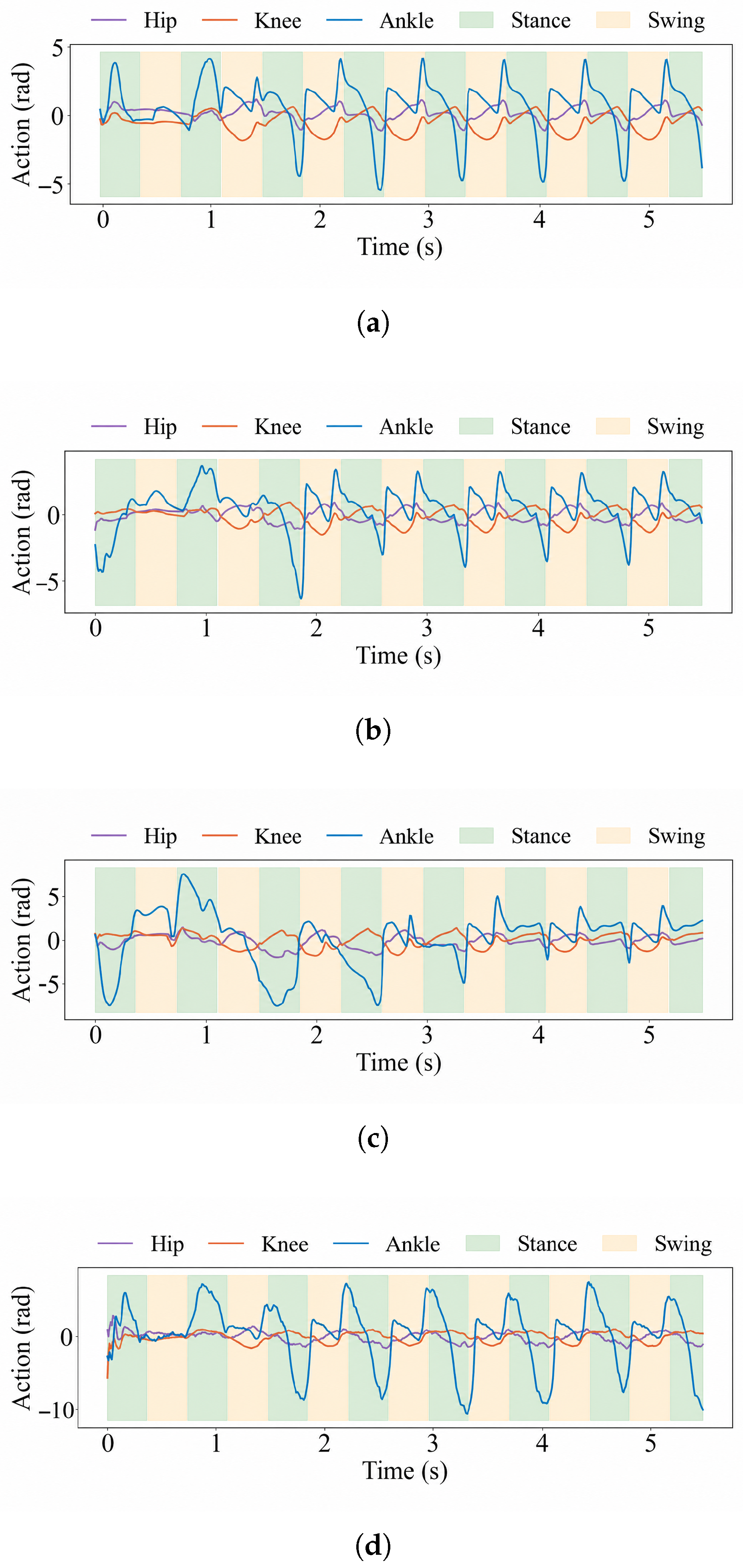
To systematically analyze the performance differences at the low-level control layer, we compared the policy action outputs of RSR, EIWM, IWM, and RMA under a 1.5 m/s velocity command. Figure 12 presents the action trajectories of each algorithm, and

Table 12. Standard deviations of joint actions for different methods.

Method	Hip Joint (rad)	Knee Joint (rad)	Ankle Joint (rad)
RMA	0.7447	0.7546	4.2153
IWM	0.7125	0.7956	3.1262
EIWM	0.4996	0.5974	1.7028
RSR	0.4863	0.5857	1.6957

reports the standard deviations of actions for each joint.

The experimental results indicate that RSR, EIWM, and IWM generally outperform the RMA method, exhibiting smaller fluctuations in joint actions. For RSR, the standard deviations of the hip, knee, and ankle joints are 0.4863 rad, 0.5857 rad, and 1.6957 rad, respectively, either surpassing or closely matching the best values among the other methods. While EIWM and IWM produce relatively stable joint outputs, some local irregular fluctuations remain. Analysis based on the smoothness metric $Sm$ further corroborates this finding. For RSR, the $Sm$ values of the hip, knee, and ankle joints are 0.156, 0.182, and 0.311, respectively, indicating that the control signals are dominated by low-frequency components and that high-frequency oscillations are effectively suppressed. EIWM and IWM show slightly higher $Sm$ values but still significantly outperform RMA, which exhibits the poorest action smoothness with large-amplitude, high-frequency oscillations. The advantage of RSR lies in leveraging the torque refinement strategy during locomotion control training to reduce the discrepancy in real robot dynamics, thereby suppressing unnecessary high-frequency components caused by model errors and policy redundancy, and improving both the smoothness and temporal continuity of actions. In contrast, while EIWM and IWM improve overall action stability, they cannot completely eliminate high-frequency oscillations, and RMA shows pronounced joint fluctuations and high-frequency instability. Overall, combining explicit–implicit learning with the RS stage effectively mitigates joint oscillation issues caused by the sim2real gap.

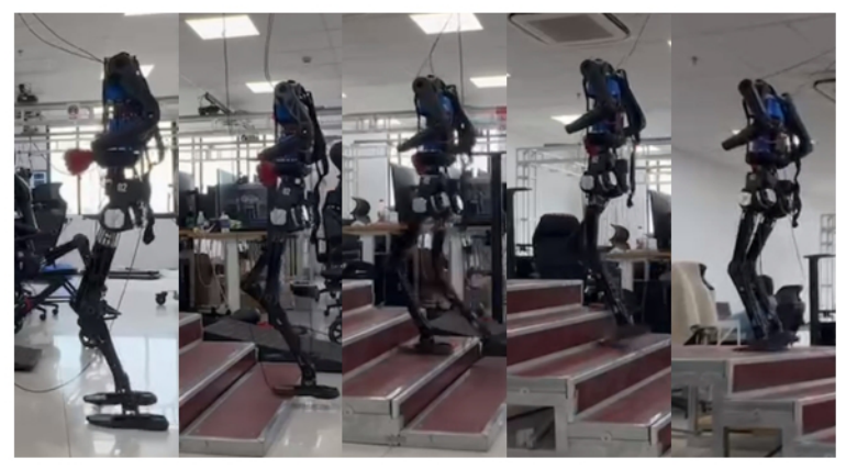
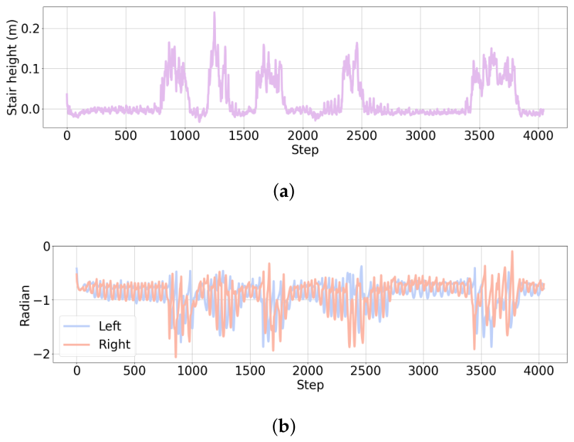
The robot was tested on a staircase consisting of four consecutive steps, each with a height of 12 cm, as shown in Figure 13. During the experiment, the robot first walked on flat ground and then proceeded to ascend the stairs.

Figure 14 illustrates the relationship between the explicitly estimated terrain height and the knee joint motion. The results indicate that the RSR method can accurately capture changes in the stair height. When the estimated terrain height increases, the robot correspondingly increases the knee flexion angle to achieve sufficient foot clearance and successfully step over the stair; during flat-ground walking, as the estimated terrain height varies only slightly, the knee joint makes minimal adjustments to maintain a low foot lift while walking. It is noteworthy that the terrain height is privileged information and cannot be directly measured by the robot’s sensors in the real environment.

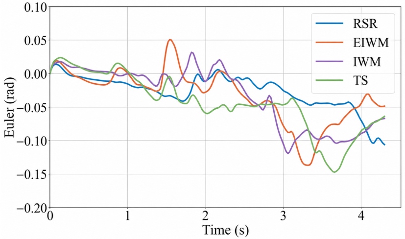
For the typical complex terrain task of stair climbing, the performance of RSR, EIWM, IWM, and RMA in controlling the robot’s body pitch angle was systematically evaluated. The corresponding trajectories are shown in Figure 15.

Based on the statistical metrics in

Table 13. Comparison of robot pitch stability during stair climbing across different methods.

Method	Mean (rad)	Std. Dev. (rad)	Max Abs. (rad)
RMA	−0.0434	0.0431	0.1471
IWM	−0.0334	0.0446	0.1191
EIWM	−0.0321	0.0395	0.1367
RSR	−0.0262	0.0255	0.1065

, the RSR method achieves an average pitch Euler angle of −0.0262 rad, which is closest to the horizontal state. The standard deviation and the maximum absolute value of the pitch angle for RSR are only 0.0255 rad and 0.1065 rad, respectively. Compared with the suboptimal EIWM method, RSR reduces the absolute value of the mean, the standard deviation, and the maximum absolute value of the pitch angle by 18.4%, 35.4%, and 22.1%, respectively. Relative to the IWM and RMA methods, RSR demonstrates even more pronounced advantages: the absolute values of the mean decrease by 21.6% and 39.6%, the standard deviations decrease by 42.8% and 40.8%, and the maximum absolute values decrease by 10.6% and 27.6%, respectively. Across all four metrics, RSR outperforms all comparison methods, highlighting its superior performance in attitude stability and control robustness. This outstanding performance mainly benefits from the RS stage in RSR, which effectively reduces the sim-to-real discrepancy. In contrast, although EIWM improves control performance through explicit–implicit learning, its mean pitch and fluctuation magnitude are still slightly inferior to RSR, indicating that the absence of a torque regularization strategy limits its generalization to the robot’s time-varying dynamics. Since IWM and RMA do not incorporate explicit estimation of key information, their pitch fluctuations are significantly larger, particularly during instantaneous transitions on the stairs, reflecting their insufficient dynamic response to complex terrain.

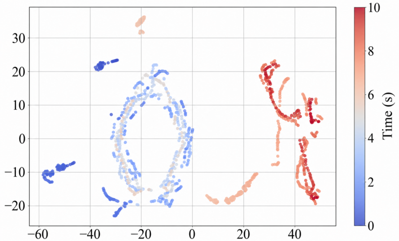
Under both flat ground and stair terrain conditions, the implicit representation space of the RSR method exhibits a clear clustering structure, as shown in Figure 16. Overall, the implicit space can be divided into two distinct clusters, corresponding to flat-ground walking and stair climbing. It is noteworthy that during the transition phase from flat ground to stairs, there is partial overlap in the implicit representations. This phenomenon primarily arises because the implicit space is constructed solely from proprioceptive observations, without incorporating any external environmental sensing. During the transition phase, since the robot has not yet sufficiently engaged with the stairs, its proprioceptive state is highly similar to that of flat-ground walking, leading to overlapping implicit representations. The clustering observed in the implicit space indicates that the RSR method can effectively distinguish terrain features using historical proprioceptive observations, thereby enhancing the interpretability of the policy behavior. Furthermore, the implicit representation provides the policy with a low-dimensional, structured form of environment representation, enabling adaptive behavior in various unstructured terrains.

Overall, RMA benefits from its teacher–student training framework but relies on privileged information and multi-stage training. IWM adopts a purely implicit representation and exhibits limited adaptability to complex terrains. EIWM improves training efficiency and locomotion performance by combining explicit estimation with implicit representation; however, it does not address the proprioceptive dynamics gap during sim2real transfer. Building upon EIWM, RSR further introduces the RS-stage torque refinement policy to model the time-varying dynamics of the tendon-driven system, achieving the best overall performance in both simulation and real-world experiments. The results demonstrate that the explicit–implicit learning paradigm enhances locomotion capability, while the RS-stage dynamics modeling further improves sim2real transfer performance.

5.3. Multi-Scenario Locomotion Control Experiments

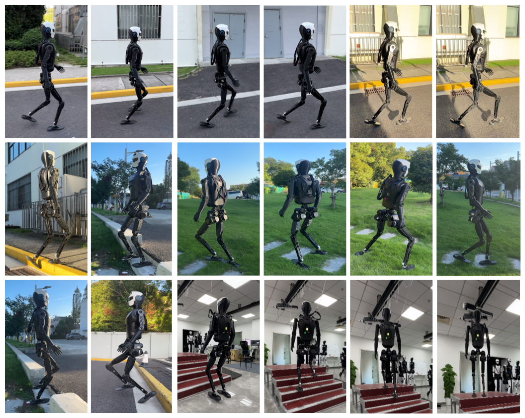
The real-world locomotion test scenarios for the robot are shown in Figure 17. To comprehensively evaluate the motion capability and environmental adaptability of the proposed method in real environments, the experiments included a variety of representative challenging terrains and high-dynamics tasks, such as: running at 2.5 m/s on asphalt, stepping over 20 cm discrete obstacles, continuously ascending a two-step 10 cm staircase, walking on soft sloped grass, and climbing four consecutive 12 cm stairs. These test scenarios cover typical challenges including high-speed locomotion, discrete obstacles, inclined surfaces, and non-rigid contact terrains, providing a comprehensive assessment of the robot’s overall locomotion control performance in real-world conditions.

The experimental results indicate that the RSR method maintains stable locomotion across all scenarios. During high-speed walking at 2.5 m/s, the robot preserves good posture stability and velocity-tracking performance. When traversing discrete steps and staircases, the implicit representation can accurately capture sudden terrain changes. In environments with uncertain contact conditions, such as soft grass, the robot still walks stably without slipping, losing balance, or interrupting its gait. Notably, the soft grass scenario was not included in the simulation training environment, and its contact characteristics and ground deformation differ significantly from the training domain. The RSR method is still able to achieve stable walking in this scenario, demonstrating that the proposed approach not only adapts to terrains seen in simulation training but also possesses cross-scenario generalization and robustness in real-world environments. This further validates the role of the torque residual policy in mitigating the time-varying dynamics differences of the robot and the effectiveness of the combined explicit–implicit learning approach in enhancing environmental adaptability.

6. Conclusions

We propose an RSR framework for bipedal robot locomotion learning. The torque refinement policy network in the RS stage effectively reduces the proprioceptive dynamics gap during sim2real transfer for tendon-driven robots, while the explicit–implicit learning approach enhances walking performance and adaptability across diverse environments. Experiments on unstructured terrains, including grass, stairs, and irregular surfaces, demonstrate the method’s stable walking capability. Results show that the robot can consecutively climb a four-step staircase with 12 cm step height and achieve stable high-speed walking at 2.5 m/s. The implicit representation space exhibits distinct clustering patterns across different terrains, indicating that the RSR method can effectively distinguish state features from historical proprioceptive observations, thereby improving walking adaptability. In real-world experiments, the explicit–implicit learning approach reduces velocity tracking errors by 15.9% compared to a purely implicit baseline at 2.5 m/s, and incorporating the torque refinement policy further reduces the error by 86.4%, demonstrating the RSR framework’s superior velocity tracking capability. In future work, we plan to incorporate visual information to enable robust locomotion over more complex terrains. At the same time, we aim to integrate adversarial motion priors to achieve biologically inspired gait, and utilize biologically inspired gait trajectories during the RS stage to train the torque refinement policy, further enhancing the robot’s locomotion performance and environmental adaptability.

References

1. Tang, J.; Mou, H.; Hou, Y.; Zhu, Y.; Liu, J.; Zhang, J. A Low-Inertia and High-Stiffness Cable-Driven Biped Robot: Design, Modeling, and Control. Mathematics 2024, 12, 559. [Google Scholar]
2. Lin, B.; Wang, J.; Song, S.; Li, B.; Meng, M.Q.H. A modular lockable mechanism for tendon-driven robots: Design, modeling and characterization. IEEE Robot. Autom. Lett. 2022, 7, 2023–2030. [Google Scholar] [CrossRef]
3. Lens, T.; von Stryk, O. Design and dynamics model of a lightweight series elastic tendon-driven robot arm. In Proceedings of the 2013 IEEE International Conference on Robotics and Automation, Karlsruhe, Germany, 6–10 May 2013; pp. 4512–4518. [Google Scholar]
4. Guist, S.; Schneider, J.; Ma, H.; Chen, L.; Berenz, V.; Martus, J.; Ott, H.; Grüninger, F.; Muehlebach, M.; Fiene, J.; et al. Safe & Accurate at Speed with Tendons: A Robot Arm for Exploring Dynamic Motion. In Proceedings of the RSS 2024 Workshop: Data Generation for Robotics, Delft, The Netherlands, 15 July 2024. [Google Scholar]
5. Zhang, Q.; Li, C.; Jing, H.; Li, H.; Li, X.; Ju, H.; Tang, Y.; Zhao, J.; Zhu, Y. Rtsras: A series-parallel-reconfigurable tendon-driven supernumerary robotic arms. IEEE Robot. Autom. Lett. 2022, 7, 7407–7414. [Google Scholar]
6. Li, H.; Ford, C.J.; Bianchi, M.; Catalano, M.G.; Psomopoulou, E.; Lepora, N.F. BRL/Pisa/IIT SoftHand: A low-cost, 3D-printed, underactuated, tendon-driven hand with soft and adaptive synergies. IEEE Robot. Autom. Lett. 2022, 7, 8745–8751. [Google Scholar]
7. Lange, F.; Pfanne, M.; Steinmetz, F.; Wolf, S.; Stulp, F. Friction estimation for tendon-driven robotic hands. In Proceedings of the 2021 IEEE International Conference on Robotics and Automation (ICRA), Xi’an, China, 30 May–5 June 2021; pp. 6505–6511. [Google Scholar]
8. Duan, H.; Pandit, B.; Gadde, M.S.; Van Marum, B.; Dao, J.; Kim, C.; Fern, A. Learning vision-based bipedal locomotion for challenging terrain. In Proceedings of the 2024 IEEE International Conference on Robotics and Automation (ICRA), Yokohama, Japan, 13–17 May 2024; pp. 56–62. [Google Scholar]
9. van Marum, B.; Shrestha, A.; Duan, H.; Dugar, P.; Dao, J.; Fern, A. Revisiting reward design and evaluation for robust humanoid standing and walking. In Proceedings of the 2024 IEEE/RSJ International Conference on Intelligent Robots and Systems (IROS), Abu Dhabi, United Arab Emirates, 14–18 October 2024; pp. 11256–11263. [Google Scholar]
10. Ha, S.; Lee, J.; van de Panne, M.; Xie, Z.; Yu, W.; Khadiv, M. Learning-based legged locomotion: State of the art and future perspectives. Int. J. Robot. Res. 2024, 44, 1396–1427. [Google Scholar]
11. Choi, S.; Ji, G.; Park, J.; Kim, H.; Mun, J.; Lee, J.H.; Hwangbo, J. Learning quadrupedal locomotion on deformable terrain. Sci. Robot. 2023, 8, eade2256. [Google Scholar] [CrossRef] [PubMed]
12. Tan, J.; Zhang, T.; Coumans, E.; Iscen, A.; Bai, Y.; Hafner, D.; Bohez, S.; Vanhoucke, V. Sim-to-Real: Learning Agile Locomotion for Quadruped Robots. arXiv 2018, arXiv:1804.10332. [Google Scholar]
13. Hwangbo, J.; Lee, J.; Dosovitskiy, A.; Bellicoso, D.; Tsounis, V.; Koltun, V.; Hutter, M. Learning agile and dynamic motor skills for legged robots. Sci. Robot. 2019, 4, eaau5872. [Google Scholar] [CrossRef] [PubMed]
14. Kumar, A.; Fu, Z.; Pathak, D.; Malik, J. RMA: Rapid Motor Adaptation for Legged Robots. In Proceedings of the Robotics: Science and Systems XVII, Virtual, 12–16 July 2021. [Google Scholar]
15. Kumar, A.; Li, Z.; Zeng, J.; Pathak, D.; Sreenath, K.; Malik, J. Adapting rapid motor adaptation for bipedal robots. In Proceedings of the 2022 IEEE/RSJ International Conference on Intelligent Robots and Systems (IROS), Kyoto, Japan, 23–27 October 2022; pp. 1161–1168. [Google Scholar]
16. Radosavovic, I.; Xiao, T.; Zhang, B.; Darrell, T.; Malik, J.; Sreenath, K. Real-world humanoid locomotion with reinforcement learning. Sci. Robot. 2024, 9, eadi9579. [Google Scholar] [CrossRef] [PubMed]
17. Nahrendra, I.M.A.; Yu, B.; Myung, H. DreamWaQ: Learning Robust Quadrupedal Locomotion With Implicit Terrain Imagination via Deep Reinforcement Learning. In Proceedings of the 2023 IEEE International Conference on Robotics and Automation, ICRA 2023, London, UK, 29 May–2 June 2023; pp. 5078–5084. [Google Scholar]
18. Wang, Z.; Wei, W.; Yu, R.; Wu, J.; Zhu, Q. Toward understanding key estimation in learning robust humanoid locomotion. In Proceedings of the 2024 IEEE/RSJ International Conference on Intelligent Robots and Systems (IROS), Abu Dhabi, United Arab Emirates, 14–18 October 2024; pp. 11232–11239. [Google Scholar]
19. Rao, P.; Thomas, G.C.; Sentis, L.; Deshpande, A.D. Analyzing achievable stiffness control bounds of robotic hands with coupled finger joints. In Proceedings of the 2017 IEEE International Conference on Robotics and Automation (ICRA), Singapore, 29 May–3 June 2017; pp. 3447–3452. [Google Scholar]
20. Lai, H.; Cao, J.; Xu, J.; Wu, H.; Lin, Y.; Kong, T.; Yu, Y.; Zhang, W. World model-based perception for visual legged locomotion. In Proceedings of the 2025 IEEE International Conference on Robotics and Automation (ICRA), Atlanta, GA, USA, 19–23 May 2025; pp. 11531–11537. [Google Scholar]
21. Zhang, C.; Rudin, N.; Hoeller, D.; Hutter, M. Learning agile locomotion on risky terrains. In Proceedings of the 2024 IEEE/RSJ International Conference on Intelligent Robots and Systems (IROS), Abu Dhabi, United Arab Emirates, 14–18 October 2024; pp. 11864–11871. [Google Scholar]
22. Xue, J.; Liang, Z.; Mou, H.; Li, Q.; Zhang, J. LSWM: A Long–Short History World Model for Bipedal Locomotion via Reinforcement Learning. Biomimetics 2026, 11, 40. [Google Scholar] [CrossRef] [PubMed]
23. Li, Z.; Peng, X.B.; Abbeel, P.; Levine, S.; Berseth, G.; Sreenath, K. Reinforcement learning for versatile, dynamic, and robust bipedal locomotion control. Int. J. Robot. Res. 2025, 44, 840–888. [Google Scholar]
24. He, T.; Gao, J.; Xiao, W.; Zhang, Y.; Wang, Z.; Wang, J.; Luo, Z.; He, G.; Sobanbabu, N.; Pan, C.; et al. ASAP: Aligning Simulation and Real-World Physics for Learning Agile Humanoid Whole-Body Skills. arXiv 2025, arXiv:2502.01143. [Google Scholar]
25. Mysore, S.; Mabsout, B.; Mancuso, R.; Saenko, K. Regularizing action policies for smooth control with reinforcement learning. In Proceedings of the 2021 IEEE International Conference on Robotics and Automation (ICRA), Xi’an, China, 30 May–5 June 2021; pp. 1810–1816. [Google Scholar]
Figure 1. Actuation methods and coupling relationship of the knee and ankle joints.
Mathematics 14 02358 g001
Figure 2. Overview of the proposed RSR framework.
Mathematics 14 02358 g002
Figure 3. Reinforcement learning-Based framework for modeling time-varying proprioceptive dynamics.
Mathematics 14 02358 g003
Figure 4. Sim2real framework for locomotion training, and deployment.
Mathematics 14 02358 g004
Figure 5. Illustration of the terrain curriculum for walking training.
Mathematics 14 02358 g005
Figure 6. Reward curves of the three algorithms during training.
Mathematics 14 02358 g006
Figure 7. Terrain difficulty levels during training for the three algorithms.
Mathematics 14 02358 g007
Figure 8. Average linear velocity tracking reward curves during training for the three algorithms.
Mathematics 14 02358 g008
Figure 9. Comparison of real-time learning times for the three algorithms.
Mathematics 14 02358 g009
Figure 10. Comparison of hip joint proprioceptive dynamics responses between the original simulation environment, the simulation with RS-stage torque refinement, and the real robot. (a) Low-Speed Motion; (b) High-Speed Motion.
Mathematics 14 02358 g010
Figure 11. Average linear velocity tracking under a 2.5 m/s command over five independent trials for RSR and EIWM.
Mathematics 14 02358 g011
Figure 12. Hip, knee, and ankle joint actions of four algorithms under a 1.5 m/s velocity command. (a) RSR; (b) EIWM; (c) IWM; (d) RMA.
Mathematics 14 02358 g012
Figure 13. Scenario for testing stair ascent.
Mathematics 14 02358 g013
Figure 14. Comparison of knee joint position changes with explicitly estimated terrain height during stair ascent and descent. (a) Explicitly estimated terrain height; (b) Knee joint position variation.
Mathematics 14 02358 g014
Figure 15. The variation of the robot’s pitch Euler angle during stair climbing under the four algorithms.
Mathematics 14 02358 g015
Figure 16. The implicit representation space during the transition from flat ground to stair climbing.
Mathematics 14 02358 g016
Figure 17. Illustration of robot locomotion experiments on complex indoor and outdoor terrains.
Mathematics 14 02358 g017