A Neural Residual Correction of the Explicit Euler Method via Learned Truncation Error Operators: A Lotka–Volterra Case Study

Abstract

The explicit Euler method is widely used for the numerical integration of ordinary differential equations due to its simplicity and low computational cost; however, its accuracy and long-term qualitative behavior deteriorate for nonlinear oscillatory systems when moderate or large time steps are employed. This work proposes a neural residual correction framework for the Lotka–Volterra system, where a neural network learns a data-driven approximation of the local truncation error of the Euler scheme relative to a sixth-order Taylor reference solution (Taylor6). The learned correction is incorporated into the Euler update, yielding a hybrid integrator that preserves the simplicity of the base method while improving accuracy and long-term boundedness. Separate neural networks are trained for fixed time-step sizes, with emphasis on an intermediate regime ($\Delta t\approx 0.8$–$1.1$) where the standard Euler method exhibits pronounced qualitative distortions. Numerical experiments show that the corrected method reduces phase and amplitude errors, preserves the qualitative structure of phase portraits, and generalizes to previously unseen parameter configurations. Comparisons with the classical fourth-order Runge–Kutta method further illustrate the robustness of the proposed approach in this regime. Unlike previous neural correction approaches focused on small time steps, high-order solvers, or global solution operators, the proposed framework specifically targets the intermediate regime where Euler’s truncation error becomes qualitatively dominant while remaining sufficiently structured to be learned through residual correction. Throughout this work, the term “stability” is used exclusively in a qualitative sense, referring to long-term boundedness and phase-portrait preservation.

1. Introduction

Numerical integration of ordinary differential equations (ODEs) is fundamental for modeling and simulating dynamical systems in biology, physics, and engineering [1,2]. Among available numerical schemes, the explicit Euler method is widely used for its simplicity and low computational cost, but suffers from accuracy and long-term qualitative limitations, especially in nonlinear oscillatory systems or for moderate to large time steps [3].

The Lotka–Volterra system [4,5] is a classical benchmark for such limitations. Small time steps allow Euler to produce reasonable approximations, but intermediate or large steps result in phase distortion, amplitude errors, and potentially spurious divergence. High-order methods such as Taylor expansions or Runge–Kutta alleviate these issues but increase computational cost per step [2].

Hybrid approaches combining classical numerical integration with machine learning have recently emerged, aiming to improve accuracy, long-term qualitative behavior, or efficiency by learning problem-dependent corrections from data. Representative examples include residual correction frameworks, solver-informed neural networks, and physics-informed architectures that learn discrepancies between low-fidelity approximations and high-order references [6,7,8,9].

Motivated by this perspective, we propose a neural residual correction framework to augment the explicit Euler method. The network learns the local truncation error relative to a high-order Taylor reference, which is then added to the Euler step. This yields a hybrid integrator that retains the simplicity of Euler while substantially improving accuracy and long-term boundedness in intermediate time-step regimes where Euler alone fails.

Unlike prior neural correction strategies focused on high-order solvers or global solution operators, [10,11] our framework targets the explicit Euler method in a regime where it becomes qualitatively unreliable but remains numerically bounded. Rather than learning the full dynamics, the neural network approximates the dominant truncation-error operator, providing a numerically interpretable correction connected to modified equation theory and backward error analysis.

Recent advances in scientific machine learning emphasize using neural networks to approximate structured discrepancies in physical or numerical models rather than replacing the underlying equations [7,12,13]. In this context, our work is a specific and interpretable instance of this paradigm, where the network learns the local truncation error of Euler relative to a high-order reference, situating the approach within a broader class of data-driven model-correction methods. Recent studies have also investigated computational aspects of explicit numerical methods, including parallel implementations that improve efficiency while preserving the simplicity of low-order schemes. For example, Koics et al. [14] analyzed OpenCL-based parallelization strategies for explicit methods applied to the heat equation, demonstrating that computational performance remains an important consideration when evaluating enhanced numerical integrators. This perspective is particularly relevant in the present work, where neural correction improves accuracy while introducing an additional computational overhead compared with the standard Euler method.

The main contributions of this work are:

• We introduce a neural residual correction framework that augments the explicit Euler method by learning its local truncation error relative to a high-order Taylor reference.
• We demonstrate substantial improvements in accuracy and long-term boundedness in an intermediate time-step regime where classical Euler integration degrades.
• We show that the neural-corrected method generalizes across unseen parameter configurations while producing trajectories comparable to higher-order integrators.
• We provide a detailed analysis of computational cost, qualitative behavior, and practical trade-offs, situating the approach within the broader context of data-driven hybrid numerical methods.

2. The Lotka–Volterra System

The Lotka–Volterra equations describe the interaction between two species: a prey population $N\left(t\right)$ and a predator population $P\left(t\right)$, where t represents time. This system of ordinary differential equations was independently proposed by Alfred J. Lotka (1925) and Vito Volterra (1926) [4,5] and remains one of the cornerstone models for studying predator–prey dynamics.

The classical form of the model is given by

$$\begin{array}{cc}\hfill {\displaystyle \frac{dN}{dt}}& =aN-bNP,\hfill \\ \hfill {\displaystyle \frac{dP}{dt}}& =-cP+dNP,\hfill \end{array}$$

(1)

where the positive parameters have the following biological interpretation:

• $a>0$: intrinsic growth rate of the prey population,
• $b>0$: predation (interaction) rate,
• $c>0$: natural mortality rate of the predator population,
• $d>0$: conversion efficiency of consumed prey into predator population growth.

System (1) admits two equilibrium points:

$$(N_1^{*},P_1^{*})=(0,0),(N_2^{*},P_2^{*})=\left({\displaystyle \frac{c}{d}},{\displaystyle \frac{a}{b}}\right).$$

The origin is unstable, whereas the second equilibrium is a center that generates closed periodic orbits around it. These persistent oscillations constitute one of the most distinctive features of the model and make it a standard benchmark for evaluating numerical integration methods and modern approximation techniques.

In the present work, multiple configurations of the system are considered by varying both the parameters $(a,b,c,d)$ and the initial conditions $(N_0,P_0)$. This strategy produces a rich and diverse set of dynamical behaviors ranging from weakly damped to large-amplitude limit cycles. The resulting simulations form the synthetic dataset used to train a residual neural network whose objective is to learn a correction to the explicit Euler method, thereby dramatically improving its accuracy by predicting the residual between the Euler step and a high-precision integrator (Taylor series method of order 6).

The Lotka–Volterra system is not chosen for biological realism, but as a canonical conservative oscillatory system with a known invariant structure, making it ideal for assessing long-term qualitative degradation induced by numerical schemes.

3. Numerical Time Integration Methods

To benchmark the performance of the proposed neural corrector against classical numerical integration schemes, the Lotka–Volterra system is solved using three fixed-step methods: the explicit Euler method, a high-order Taylor series method, and the classical fourth-order Runge–Kutta method (RK4).

A sixth-order Taylor method (Taylor6) is used as a numerical surrogate reference, not as an exact solution, and is assumed sufficiently accurate within the considered admissible time-step regime [2]. Owing to its high order of accuracy, this method provides a reliable approximation of the true trajectory within this regime. In this work, Taylor6 serves two purposes: (i) the generation of synthetic datasets used to train and validate the neural corrector, and (ii) the quantitative evaluation of numerical errors produced by both the explicit Euler method and its neural-corrected counterpart. Importantly, Taylor6 is used as a numerical reference rather than an exact ground-truth solution.

3.1. Explicit Euler Method

The explicit Euler method is the simplest first-order time integration scheme and is defined by the recurrence

$$y_{n+1}=y_n+hf(t_n,y_n),$$

(2)

where h denotes the time step, $y_n={[N_n,P_n]}^{\top }$ is the state vector, and f represents the Lotka–Volterra dynamics.

Due to its low computational cost and straightforward implementation, the explicit Euler method is frequently used as a baseline integrator. However, its limited accuracy and poor long-term qualitative behavior make it unsuitable for long-time integration of nonlinear oscillatory systems unless very small time steps are employed.

3.1.1. Error Structure and Dependence on the Time Step

The explicit Euler method has a local truncation error of order $O\left(h^2\right)$ and a global accumulated error of order $O\left(h\right)$ [2]. Consequently, the numerical error grows linearly with the time step size, making the method highly sensitive to moderate and large values of h.

For nonlinear dynamical systems such as the Lotka–Volterra equations, this error manifests not only as a loss of pointwise accuracy, but also as systematic distortions in the qualitative behavior of the solution. In particular, Euler’s method tends to introduce phase lag and amplitude drift in oscillatory trajectories, which accumulate over time and alter the long-term dynamics.

3.1.2. Boundedness Considerations for Oscillatory Dynamics

From the perspective of classical linear analysis, the explicit Euler method possesses a limited boundedness region. For the linear test equation $y^{\prime }=\lambda y$, bounded trajectories require

$$|1+h\lambda |<1,$$

(3)

which severely restricts the admissible time step when $\lambda$ has a non-negligible imaginary component [2,15].

Although the Lotka–Volterra system is nonlinear, its linearization around equilibrium points exhibits oscillatory behavior with complex eigenvalues. As a result, explicit Euler integration with moderate or large time steps often produces numerical artifacts such as artificial damping, spurious growth, or distortion of the phase portrait, even when pointwise errors remain moderate over short time intervals.

3.1.3. Impact of the Sampling Interval $\Delta t$

In this work, the numerical solution is sampled at a larger interval $\Delta t$, which may differ from the internal integration step used to generate reference solutions. As $\Delta t$ increases, the discrepancy between the explicit Euler approximation and higher-order reference methods becomes more pronounced.

For small values of $\Delta t$, the error introduced by Euler’s method remains comparable to that of higher-order schemes, and the benefit of correction is limited. However, for moderate to large $\Delta t$, the accumulated truncation error becomes structured and systematic, rather than purely stochastic. This regime is particularly suitable for data-driven correction strategies, as the error depends smoothly on the state, system parameters, and time step.

3.1.4. Motivation for Neural Error Correction

The deterministic nature of Euler’s truncation error suggests that it can be approximated as a function of the current state, model parameters, and time step size. This observation motivates the use of data-driven correction strategies, in which a learned model compensates for systematic discretization errors [8]. Instead of replacing the Euler method with a higher-order integrator, we propose to augment it with a neural correction term that compensates for its local truncation error, following a residual learning paradigm [16].

3.2. High-Order Taylor Methods

Taylor series methods approximate the solution by expanding it as a truncated Taylor series in time. A Taylor method of order p requires the computation of time derivatives of the vector field up to order p and exhibits a local truncation error of $O\left(h^{p+1}\right)$.

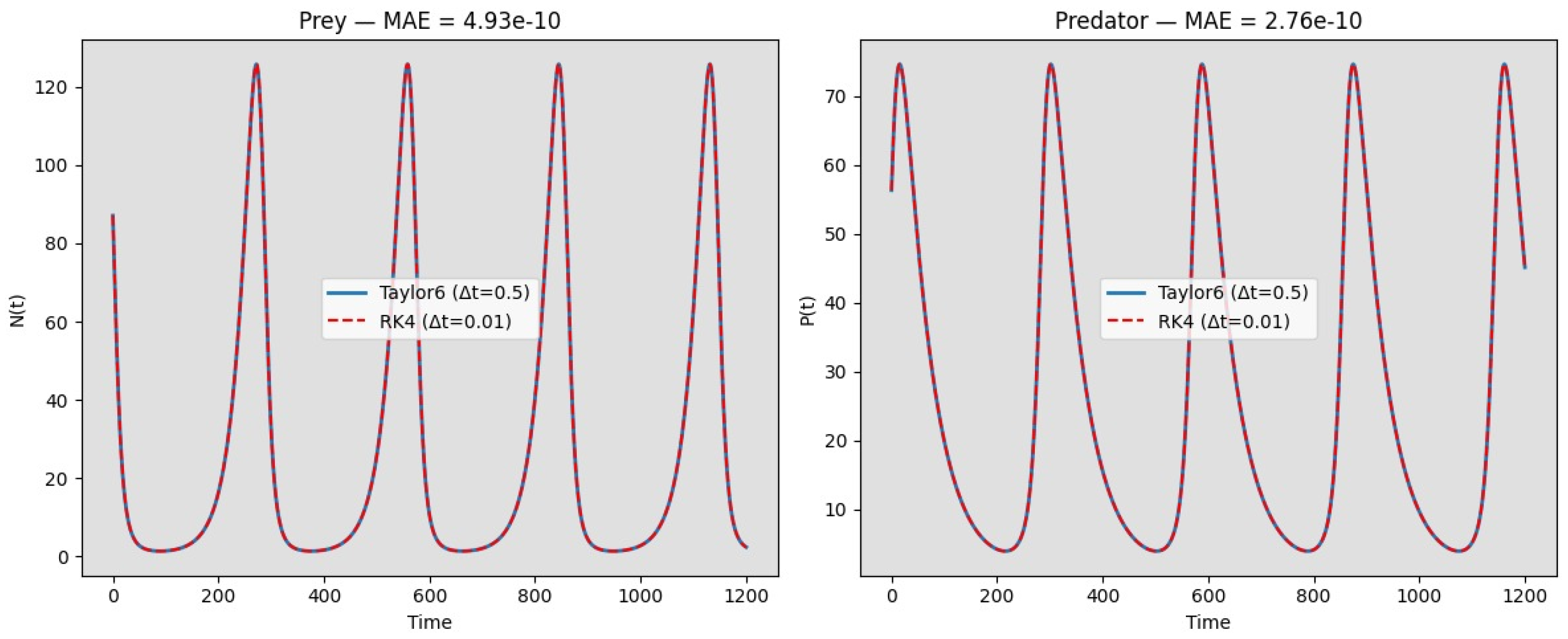
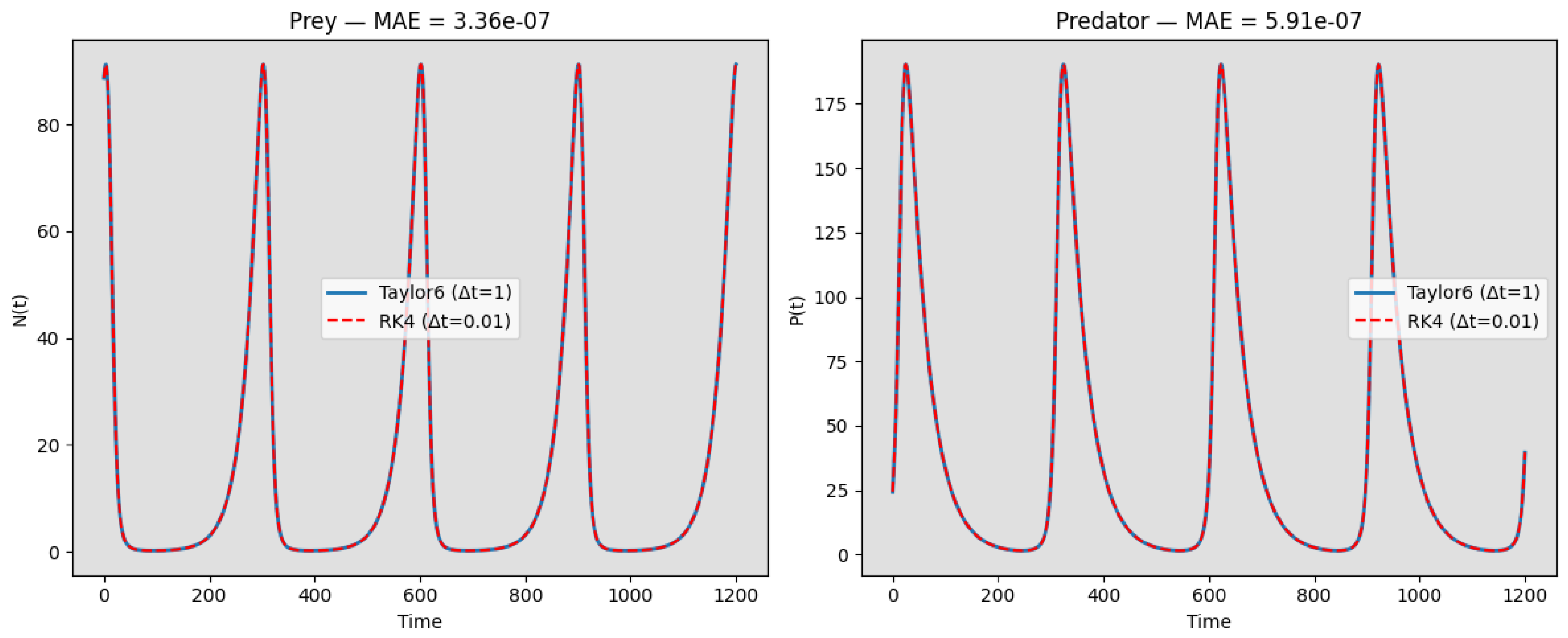
In this study, the sixth-order Taylor method serves as a numerical surrogate reference. Its accuracy is verified in Appendix A against an independent RK4 solver using a significantly smaller time step. With a local truncation error of $O\left(h^7\right)$, this method produces highly accurate trajectories for sufficiently small to moderate time steps. Despite this accuracy, the computational cost associated with evaluating higher-order derivatives renders Taylor methods impractical for routine simulations, particularly in high-dimensional or stiff systems. These characteristics justify the use of Taylor6 as a high-order numerical benchmark rather than as a baseline method for practical integration.

3.3. Runge–Kutta Methods

The classical fourth-order Runge–Kutta method (RK4) is a widely used fixed-step integrator with a local truncation error of $O\left(h^5\right)$ and a global error of $O\left(h^4\right)$. It is defined by the update

$$\begin{array}{cc}\hfill k_1& =hf(t_n,f{y}_n),\hfill \end{array}$$

(4)

$$\begin{array}{cc}\hfill k_2& =hf\left(t_n+\frac{h}{2},y_n+\frac{k_1}{2}\right),\hfill \end{array}$$

(5)

$$\begin{array}{cc}\hfill k_3& =hf\left(t_n+\frac{h}{2},y_n+\frac{k_2}{2}\right),\hfill \end{array}$$

(6)

$$\begin{array}{cc}\hfill k_4& =hf\left(t_{n+1},y_n+k_3\right),\hfill \end{array}$$

(7)

$$\begin{array}{cc}\hfill y_{n+1}& =y_n+\frac{1}{6}\left(k_1+2k_2+2k_3+k_4\right).\hfill \end{array}$$

(8)

Due to its higher order, RK4 generally yields more accurate results than the explicit Euler method for the same time step. However, its fixed-step formulation still limits its effectiveness in oscillatory systems when the time step is not sufficiently small. In this work, RK4 is not used as a training reference but rather as an additional benchmark to assess the generalization capability of the neural-corrected Euler scheme.

3.4. Summary

The explicit Euler method serves as a low-cost baseline, Taylor6 provides a high-order numerical reference, and RK4 offers an intermediate benchmark commonly used in practice. This combination enables a comprehensive evaluation of the proposed neural corrector across methods with different accuracy–cost trade-offs.

4. Methodology: Neural Corrector Framework

This section describes the proposed neural correction strategy for improving the explicit Euler method when applied to the Lotka–Volterra system in an intermediate large time-step regime. The approach is based on learning the local truncation error of Euler’s method with respect to a high-order Taylor reference solution.

Neural Correction of the Euler Step

Let $\left(N\right(t),P(t\left)\right)$ denote the exact (or high-fidelity reference) solution of the Lotka–Volterra system and let

$$(N_{\mathrm{Euler}}(t+\Delta t),P_{\mathrm{Euler}}(t+\Delta t))$$

be the approximation obtained with the explicit Euler method. We define the correction or residual as

$$\Delta \left(t\right)=\left(\begin{array}{c}{N}_{\mathrm{Taylor}6}(t+\Delta t)-N_{\mathrm{Euler}}(t+\Delta t)\\ P_{\mathrm{Taylor}6}(t+\Delta t)-P_{\mathrm{Euler}}(t+\Delta t)\end{array}\right).$$

(9)

The neural network is trained to approximate this residual, i.e.,

$$\widehat{\Delta }\left(t\right)=\mathrm{NN}\left(\mathbf{x}\left(t\right)\right)\approx \Delta \left(t\right),$$

where $\mathbf{x}\left(t\right)$ denotes a feature vector constructed from the current system state, model parameters, and time-step information, as detailed in the following sections. The corrected solution is given by

$$\left(\begin{array}{c}{N}_{\mathrm{corr}}(t+\Delta t)\\ P_{\mathrm{corr}}(t+\Delta t)\end{array}\right)=\left(\begin{array}{c}{N}_{\mathrm{Euler}}(t+\Delta t)\\ P_{\mathrm{Euler}}(t+\Delta t)\end{array}\right)+\widehat{\Delta }\left(t\right).$$

(10)

When the network accurately predicts the residual, we obtain

$$(N_{\mathrm{corr}},P_{\mathrm{corr}})(t+\Delta t)\approx (N_{\mathrm{Taylor}6},P_{\mathrm{Taylor}6})(t+\Delta t),$$

meaning that the Euler method, once corrected, behaves like a high-order integrator. This approach constitutes a residual learning scheme, analogous in spirit to ResNet architectures [16], where the network learns exclusively the component that the base explicit integrator fails to capture.

5. Dataset Generation

A synthetic dataset was constructed from numerical simulations of the Lotka–Volterra system to train and evaluate the proposed neural correction framework. The objective was to generate a diverse and representative set of local numerical errors produced by the explicit Euler method under different biological configurations and time-step sizes, enabling the neural networks to learn systematic correction patterns.

5.1. Parameter and Initial Condition Sampling

A total of 100 distinct combinations of model parameters and initial conditions were generated via uniform sampling within the following biologically plausible ranges:

• Model parameters:

  $$\begin{array}{cccc}\hfill a& \in [0.01,0.05]\hfill & \hfill & (\mathrm{prey}\mathrm{growth}\mathrm{rate}),\hfill \\ \hfill b& \in [0.0005,0.002]\hfill & \hfill & (\mathrm{predation}\mathrm{rate}),\hfill \\ \hfill c& \in [0.0005,0.002]\hfill & \hfill & (\mathrm{predator}\mathrm{mortality}\mathrm{rate}),\hfill \\ \hfill d& \in [0.01,0.03]\hfill & \hfill & (\mathrm{conversion}\mathrm{efficiency}).\hfill \end{array}$$
• Initial conditions:

  $$\begin{array}{cc}\hfill N_0& \in [50,150],\hfill \\ \hfill P_0& \in [10,60].\hfill \end{array}$$

All parameters were sampled independently, producing a wide variety of dynamical behaviors ranging from mild oscillations around equilibrium to large-amplitude predator–prey cycles. This diversity is essential to prevent the neural networks from overfitting to specific trajectories and to promote generalization across the system’s parameter space.

5.2. Time-Step Selection and Dataset Partitioning

The dataset generation process explicitly accounts for the dependence of numerical errors on the time-step size $\Delta t$. Rather than fixing a single step size, four distinct values were considered:

$$\Delta t\in \{0.5,0.8,1.0,1.1\}.$$

For each value of $\Delta t$, an independent dataset was generated using the same 100 parameter combinations, and a separate neural network was trained for each time-step size. This strategy avoids forcing a single model to learn corrections across disparate numerical regimes and allows each network to specialize in a specific stability–accuracy trade-off.

5.3. Numerical Integration for Data Generation

For each parameter combination $(a,b,c,d,N_0,P_0)$ and each selected value of $\Delta t$, the Lotka–Volterra system was integrated over a fixed time horizon using a uniform time step. At each time instant $t_i$, the following quantities were computed:

• The reference solution obtained using a sixth-order Taylor method (Taylor6),
• The predictor step obtained using the explicit Euler method.

6. Neural Network Architecture

The neural corrector is implemented as a fully connected residual neural network designed to approximate the local truncation error of the explicit Euler method applied to the Lotka–Volterra system. Rather than learning the system dynamics directly, the network predicts corrective terms that are added to the Euler update, yielding an enhanced numerical integrator.

6.1. Input Features

The input to the network is a 14-dimensional feature vector composed of model parameters, system state variables, and time-step-related quantities. Specifically, the input features are

$$\mathbf{x}=(a,b,c,d,N_0,P_0,t,N_{\mathrm{Euler}},P_{\mathrm{Euler}},\Delta t,\Delta t^{-1},\Delta t^2,\Delta t^3,log(\Delta t)).$$

This selection enables the network to capture both local and global properties of the dynamical system. Including $(N_0,P_0)$ allows the network to implicitly identify the orbit scale and long-term energy level of the trajectory.

6.2. Remark on the Inclusion of Initial Conditions

Although the Lotka–Volterra system is autonomous and the current state $(N,P)$ uniquely determines the future exact solution, the local truncation error of the Euler method is not a function of the current state alone. It also depends on the global orbit scale (e.g., the amplitude of oscillations), which is determined by the conserved quantity associated with the initial conditions. Two different initial conditions can lead to the same current state $(N,P)$ at different phases of their respective orbits, yet the Euler truncation error differs because the curvature of the trajectory and the higher-order derivatives of the flow depend on the orbit’s energy. Including $(N_0,P_0)$ as global trajectory-level features provides the network with the necessary context to distinguish among orbits and correctly estimate the local error. Ablation experiments confirmed that omitting $(N_0,P_0)$ degrades correction accuracy, especially for unseen parameter combinations. The inclusion of higher-order transformations of the time step is motivated by the theoretical dependence of the local truncation error of the Euler method on powers of $\Delta t$.

6.3. Output Definition

The network outputs a two-dimensional vector corresponding to the correction terms for the prey and predator populations:

$$\widehat{\Delta }=\left(\begin{array}{c}{\widehat{\Delta }}_N\\ {\widehat{\Delta }}_P\end{array}\right)=\left(\begin{array}{c}{N}_{\mathrm{Taylor}}-N_{\mathrm{Euler}}\\ P_{\mathrm{Taylor}}-P_{\mathrm{Euler}}\end{array}\right).$$

These predicted residuals are added to the Euler solution at each time step, resulting in a corrected numerical approximation of the system state.

6.4. Network Architecture

The network consists of an input layer followed by three residual blocks and a linear output layer. The input layer maps the 14-dimensional feature vector to a latent space of 256 neurons. Each residual block contains two fully connected layers with 256 neurons and identity skip connections. Layer normalization is applied after each residual addition to improve training stability. In total, the architecture comprises eight fully connected layers.

6.5. Architecture Design Considerations

The neural corrector is implemented as a fully connected residual network inspired by ResNet-type architectures [17]. The choice of a residual architecture is motivated by the nature of the learning task itself: rather than approximating the full solution of the dynamical system, the network is trained to learn only the residual error introduced by the explicit Euler method. This formulation transforms the problem into a structured residual learning task, where the target function corresponds to the local truncation error operator of the numerical integrator.

The architecture consists of an input projection layer followed by three residual blocks and a final linear output layer. Each residual block contains two fully connected layers with 256 neurons and identity skip connections. The hidden layers employ the SiLU activation function, selected for its smoothness and stable optimization behavior in continuous dynamical systems. Layer normalization is applied after each residual addition to improve gradient flow and training stability, particularly for large time-step regimes where the truncation error becomes strongly nonlinear.

Importantly, the proposed architecture should not be interpreted as a universal neural solver for arbitrary dynamical systems. The network learns corrections associated with the specific truncation-error structure generated by the explicit Euler method for the considered family of Lotka–Volterra trajectories. Nevertheless, the correction framework itself is not restricted to predator–prey systems. In principle, the same residual-learning strategy could be applied to other nonlinear ordinary differential equations, provided that suitable training data are generated from a reliable high-order reference integrator.

For different systems, however, the neural network would generally require retraining, since the structure of the local truncation error depends strongly on the underlying vector field, the qualitative dynamics, and the numerical stability properties of the system. Chaotic systems, stiff systems, or systems exhibiting sharp transitions may require modified architectures, additional features, or different training strategies.

6.6. Activation Functions and Initialization

All hidden layers employ the SiLU (Sigmoid Linear Unit) activation function, chosen for its smoothness and suitability for learning continuous corrections in dynamical systems. The weights of the input layer are initialized using Kaiming uniform initialization, while the remaining layers use default PyTorch version 2.6.0. initialization. The network is trained to minimize the mean squared error between the predicted and true correction terms, with both inputs and targets normalized to zero mean and unit variance.

6.7. Training Procedure

6.7.1. Parameter Space and Data Generation

Training data are generated using multiple combinations of the Lotka–Volterra parameters $(a,b,c,d)$ and initial conditions $(N_0,P_0)$, sampled uniformly within predefined admissible ranges. In total, 100 distinct parameter configurations are considered, each corresponding to a unique realization of $(a,b,c,d,N_0,P_0)$. These configurations are split into disjoint training, validation, and test sets to ensure genuine parametric generalization.

For each parameter configuration, the system is integrated over a fixed time horizon, producing 1000 consecutive time steps. At each time step, two numerical solutions are computed: (i) a high-order reference solution obtained using a sixth-order Taylor method (Taylor6), and (ii) a first-order predictor obtained using the explicit Euler method with the same time step $\Delta t$.

This procedure yields

$$100\mathrm{parameter}\mathrm{configurations}\times 1000\mathrm{time}\mathrm{steps}=100,000\mathrm{training}\mathrm{samples}.$$

Separate datasets are generated independently for each time-step size $\Delta t\in \{0.5,0.8,1.0,1.1\}$, and a distinct neural corrector is trained for each value of $\Delta t$ to ensure long-term boundedness and specialization.

6.7.2. Data Splitting

The dataset is randomly divided into training (70%), validation (15%), and test (15%) subsets, ensuring that parameter combinations in the test set are not seen during training.

6.7.3. Loss Function and Optimization

The network is trained by minimizing the mean squared error (MSE) loss between predicted and true normalized residuals:

$$\mathcal{L}={\displaystyle \frac{1}{M}}{\displaystyle \sum _{i=1}^M}{\parallel {\widehat{\mathbf{r}}}_i-{\mathbf{r}}_i\parallel }_2^2.$$

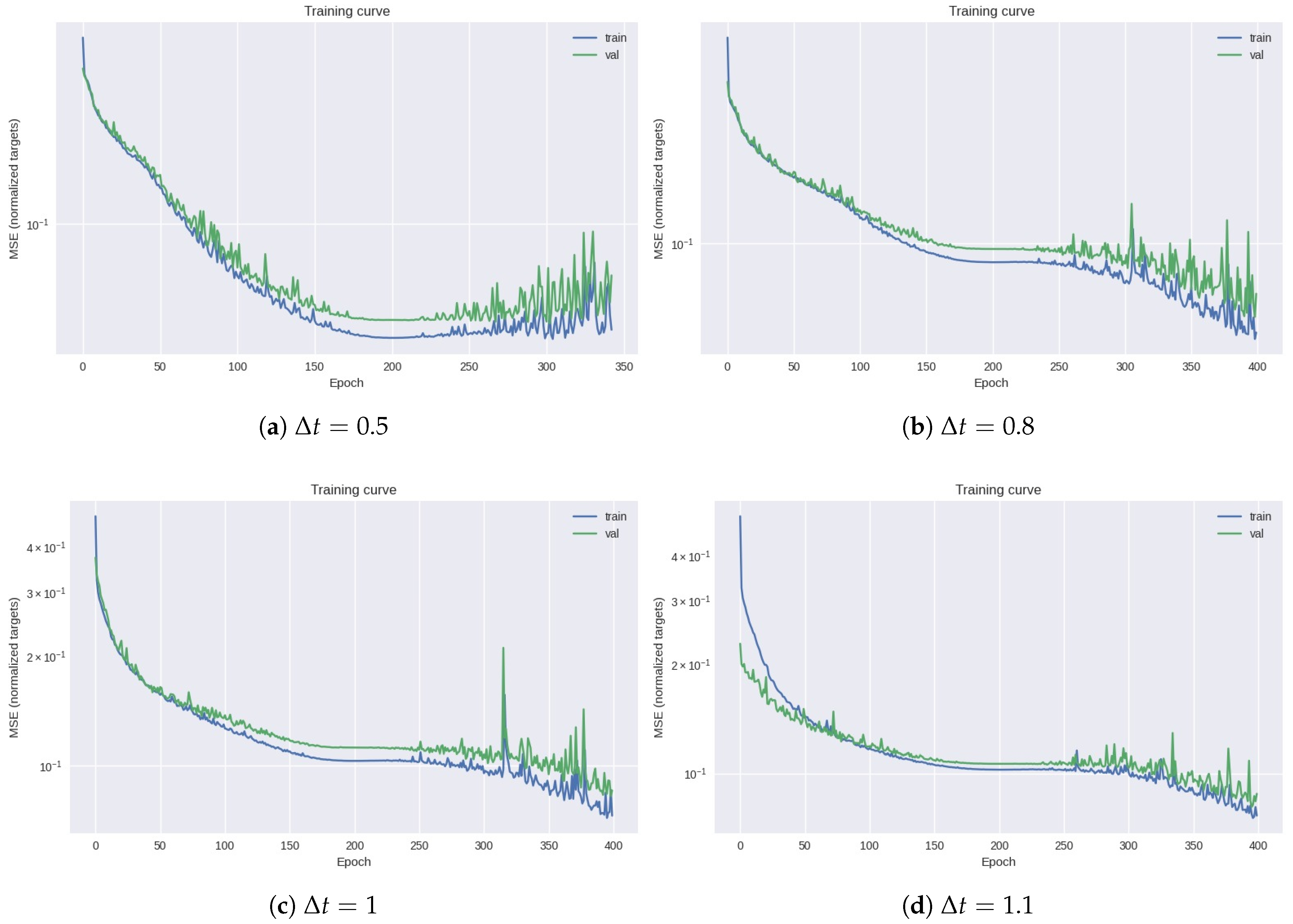
Optimization is performed using the Adam optimizer with an initial learning rate of $5\times {10}^{-4}$. A cosine annealing learning rate scheduler is employed, and early stopping is applied based on the validation loss with a patience of 40 epochs.

Figure 1 shows the evolution of training and validation loss for different values of $\Delta t$.

6.8. Neural-Corrected Euler Scheme

Algorithm 1 summarizes the proposed neural-corrected Euler scheme. At each time step, a standard explicit Euler update is first computed. A feature vector is then constructed using the current system state, the Euler prediction, the model parameters, and the time-step size. The trained neural network predicts a correction term that approximates the local truncation error of the Euler method. This correction is subsequently added to the Euler update, yielding an enhanced numerical approximation of the system trajectory.

Algorithm 1: Neural-Corrected Explicit Euler Method

The neural corrector operates on a feature vector $\Phi$ that encodes the local state of the system, model parameters, and time-step information. Specifically, the input features include the Lotka–Volterra parameters $(a,b,c,d)$, global initial conditions $(N_0,P_0)$ associated with the trajectory, the current time $t_n$, the explicit Euler prediction $(N_n^E,P_n^E)$, and several functions of the time step $\Delta t$, namely $\Delta t$, $\Delta t^{-1}$, $\Delta t^2$, $\Delta t^3$, and $log(\Delta t)$.

The quantities $(N_0,P_0)$ are treated as global trajectory-level features and remain constant throughout the integration process, while $t_n$ provides temporal context for the local correction. Although the Lotka–Volterra system is autonomous and the current state theoretically determines the local dynamics, preliminary experiments indicated that including trajectory-level information through the initial conditions improved the robustness and generalization of the neural corrector across trajectories with different oscillation amplitudes and parameter regimes. From this perspective, $(N_0,P_0)$ should be interpreted as auxiliary contextual features rather than essential dynamical variables.

Here, the feature mapping $\Phi (·)$ aggregates both local state information and global trajectory-level parameters. This design allows the neural corrector to exploit contextual information while operating locally at each integration step.

Figure 2 illustrates the proposed neural-corrected Euler framework. At each time step, the current state of the system is first advanced using the explicit Euler method. This provisional update is not used as the final solution, but rather serves as the basis for constructing a feature vector that encodes the system parameters, the current state variables, and the time-step information.

The feature vector is then passed to a neural network trained to predict the local truncation error of the Euler method with respect to a high-order reference solution. The network output corresponds to a residual correction, which is added to the Euler update to obtain the corrected state. By learning only the structured numerical error, the neural model preserves the interpretability and simplicity of the underlying integrator while significantly improving its accuracy.

This formulation ensures that the correction operates locally at each time step and remains tightly coupled to the numerical structure of the explicit Euler method, rather than acting as a black-box surrogate for the full dynamical system.

6.9. Simplicity and Computational Cost

Although the proposed method augments the explicit Euler scheme with a neural correction term, the resulting integrator remains conceptually simple. At each time step, the algorithm performs two operations:

• A standard explicit Euler update,
• A forward pass through a pre-trained neural network.

No implicit equations, nonlinear solvers, or iterative optimization procedures are required during time integration. Once the neural network has been trained offline, the corrected method retains the fully explicit character of the original Euler scheme.

The per-step computational cost can be written as

$$C_{\mathrm{NNE}}=C_{\mathrm{Euler}}+C_{\mathrm{NN}},$$

where $C_{\mathrm{Euler}}$ denotes the cost of one evaluation of the vector field and $C_{\mathrm{NN}}$ represents the cost of a single neural-network inference.

For the low-dimensional Lotka–Volterra system considered in this work, the neural-corrected Euler method is more expensive per step than both the standard Euler and classical RK4 methods. However, the corrected integrator achieves substantially improved accuracy for moderate time-step sizes, which may reduce the total number of time steps required to reach a prescribed error tolerance. Therefore, the main contribution of the proposed framework is not to reduce the cost of a single time step, but rather to enhance the accuracy and qualitative behavior of a simple explicit integrator while preserving its straightforward implementation.

6.10. Interpretation as a Data-Driven Truncation Error Operator

Let $\dot{x}=f\left(x\right)$ be an autonomous smooth dynamical system and let ${\Phi }_{\Delta t}\left(x\right)$ denote its exact flow map at time step $\Delta t$. The explicit Euler method generates the numerical update

$$x_{n+1}^E=x_n+\Delta tf\left(x_n\right),$$

(11)

which satisfies the well-known local truncation error expansion

$${\Phi }_{\Delta t}\left(x_n\right)=x_n+\Delta tf\left(x_n\right)+\mathcal{O}(\Delta t^2).$$

(12)

In this work, the neural corrector is designed to approximate the residual

$${\mathcal{R}}_{\Delta t}\left(x_n\right):={\Phi }_{\Delta t}\left(x_n\right)-\left(x_n+\Delta tf\left(x_n\right)\right),$$

(13)

which corresponds to the local truncation error operator of the Euler method. Rather than learning the dynamics f itself, the neural network learns a data-driven approximation ${\widehat{\mathcal{R}}}_{\Delta t}$ of this residual, leading to the corrected update rule

$$x_{n+1}=x_n+\Delta tf\left(x_n\right)+{\widehat{\mathcal{R}}}_{\Delta t}\left(x_n\right).$$

(14)

For smooth systems, the residual operator admits a Taylor-type expansion

$${\mathcal{R}}_{\Delta t}\left(x_n\right)={\displaystyle \frac{\Delta t^2}{2}}{f}^{\prime }\left(x_n\right)f\left(x_n\right)+\mathcal{O}(\Delta t^3),$$

(15)

which provides a formal justification for interpreting the neural corrector as a learned approximation of higher-order terms in the local flow expansion.

6.11. Extension to Multistable Systems

Although the present study focuses on the Lotka–Volterra system, the proposed neural residual correction framework is not restricted to conservative oscillatory dynamics. The method can be applied to nonlinear systems exhibiting multiple coexisting attractors, provided that the training dataset includes representative trajectories from all relevant basins of attraction. Since the network learns the local truncation error of the explicit Euler method rather than the full system dynamics, the approach remains applicable as long as this residual depends smoothly on the state, parameters, and time-step size.

The following proposition provides a heuristic consistency argument illustrating how the learned correction approximates the local truncation error of the explicit Euler method. It is intended to convey the underlying intuition rather than to constitute a complete convergence proof. A rigorous finite-time convergence and stability result, under explicit regularity and Lipschitz assumptions, is presented in Theorem 1.

Proposition 1 (Heuristic consistency interpretation of the neural-corrected scheme).

Assume that the learned corrector ${\widehat{\mathcal{R}}}_{\Delta t}$ satisfies

$${\widehat{\mathcal{R}}}_{\Delta t}\left(x\right)=\mathcal{O}(\Delta t^2)\mathit{uniformly}\mathit{on}\mathit{compact}\mathit{sets}.$$

Then the neural-corrected Euler scheme is formally consistent of order at least two with the exact flow of the system.

Proof. 

The result follows directly from the local error expansion of the exact flow and the definition of the corrected update rule. No global convergence claim is made. □

Remark 1.

The neural-corrected Euler scheme defined in (13) can be interpreted as a data-driven perturbation of the explicit Euler method. Under mild regularity assumptions on the learned correction, it is possible to establish local accuracy and boundedness properties.

Proposition 2.

Assume that the neural correction operator ${\mathcal{R}}_{\Delta t}$ satisfies a Lipschitz-type bound of the form

$$\parallel {\mathcal{R}}_{\Delta t}\left(x\right)-{\mathcal{R}}_{\Delta t}\left(y\right)\parallel \le C\Delta t^2\parallel x-y\parallel ,$$

(16)

for all $x,y$ in a compact invariant set of the Lotka–Volterra system, where $C>0$ is a constant independent of $\Delta t$. Then, the neural-corrected Euler method achieves second-order local accuracy and preserves boundedness of trajectories over finite time intervals.

Proof. 

The explicit Euler method has a local truncation error of order $\mathcal{O}(\Delta t^2)$. By construction, the neural corrector is trained to approximate this leading-order truncation error with respect to a high-order reference solution. Condition (16) ensures that the correction does not amplify perturbations and acts as a stable second-order perturbation of the Euler update.

Standard arguments based on Grönwall-type inequalities imply that the accumulated error remains bounded over finite time horizons, provided the numerical trajectory stays within a compact set. This behavior is consistent with the empirical stability and boundedness observed in the numerical experiments reported in Section 7. □

6.12. Connection with Modified Equation Theory and Backward Error Analysis

From the perspective of classical numerical analysis, the behavior of a numerical integrator can be interpreted through its associated modified equation, as introduced in backward error analysis [18]. Rather than approximating the original differential equation $\dot{x}=f\left(x\right)$ exactly, a numerical method can be viewed as exactly integrating a nearby perturbed system of the form

$$\dot{x}=f\left(x\right)+\Delta t{g}_1\left(x\right)+\Delta t^2{g}_2\left(x\right)+\cdots ,$$

(17)

where the correction terms $g_k\left(x\right)$ encode the truncation error structure of the method.

For the explicit Euler method, the leading-order term of the modified equation is well known:

$$\dot{x}=f\left(x\right)+{\displaystyle \frac{\Delta t}{2}}{f}^{\prime }\left(x\right)f\left(x\right)+\mathcal{O}(\Delta t^2),$$

(18)

revealing that Euler introduces systematic perturbations that alter phase and amplitude properties in oscillatory systems.

The neural-corrected Euler scheme proposed in this work can be interpreted as a data-driven approximation of the modified equation flow. Rather than explicitly computing the higher-order operators $g_k\left(x\right)$ through symbolic differentiation or algebraic manipulation, the neural network learns an approximation of the induced truncation-error operator directly from data:

$${\widehat{\mathcal{R}}}_{\Delta t}\left(x\right)\approx {\Phi }_{\Delta t}\left(x\right)-\left(x+\Delta tf\left(x\right)\right).$$

In this sense, the neural corrector implicitly reconstructs the dominant higher-order terms of the modified equation associated with the Euler method, but without requiring an explicit analytical derivation. The resulting corrected scheme may therefore be viewed as an Euler method whose modified equation has been partially compensated through learning.

This interpretation clarifies why the correction is most effective in the intermediate time-step regime. In this range, the leading modified-equation terms dominate the numerical error and exhibit smooth, structured dependence on the system state and parameters. For very small time steps, these terms are negligible, while for excessively large steps the modified-equation expansion itself ceases to be informative.

From this viewpoint, the proposed method bridges classical backward error analysis and modern data-driven modeling: the neural network acts as a flexible surrogate for truncation-error operators that are traditionally derived through formal series expansions.

Theorem 1

(Consistency and finite-time stability of the neural-corrected Euler scheme). Let $x^{\prime }\left(t\right)=f\left(x\left(t\right)\right)$ with $f\in C^1\left({\mathbb{R}}^d\right)$, and let ${\Phi }_{\Delta t}\left(x\right)$ denote the exact flow map of the system over a time step $\Delta t>0$. Define the local truncation error of the explicit Euler method as

$$R_{\Delta t}\left(x\right):={\Phi }_{\Delta t}\left(x\right)-\left(x+\Delta tf\left(x\right)\right).$$

Consider the neural-corrected Euler scheme

$$x_{n+1}=x_n+\Delta tf\left(x_n\right)+{\widehat{R}}_{\Delta t}\left(x_n\right),$$

(19)

where ${\widehat{R}}_{\Delta t}$ is a learned correction operator.

Assume that there exists a compact set $K\subset {\mathbb{R}}^d$ such that ${\Phi }_t\left(K\right)\subset K$ for all $t\in [0,T]$, and that for all $x,y\in K$ the following conditions hold:

(H1)

$\parallel {\widehat{R}}_{\Delta t}\left(x\right)\parallel \le C\Delta t^2$,

(H2)

$\parallel {\widehat{R}}_{\Delta t}\left(x\right)-{\widehat{R}}_{\Delta t}\left(y\right)\parallel \le C\Delta t^2\parallel x-y\parallel$,

with a constant $C>0$ independent of $\Delta t$.

Then:

(i)

The scheme (19) is locally consistent of order at least two.

(ii)

If f is Lipschitz continuous on K with constant L, then the numerical solution satisfies

$$\parallel x\left(t_n\right)-x_n\parallel \le {\displaystyle \frac{C_T}{L}}\left(e^{LT}-1\right)\Delta t,t_n=n\Delta t\le T,$$

and the scheme is stable and bounded on the finite time interval $[0,T]$.

Proof. 

We proceed in two steps.

Step 1: Local consistency. Since $f\in C^1$, the exact flow admits the Taylor expansion

$${\Phi }_{\Delta t}\left(x\right)=x+\Delta tf\left(x\right)+O(\Delta t^2),x\in K.$$

Subtracting the corrected Euler update yields

$${\Phi }_{\Delta t}\left(x\right)-\left(x+\Delta tf\left(x\right)+{\widehat{R}}_{\Delta t}\left(x\right)\right)=R_{\Delta t}\left(x\right)-{\widehat{R}}_{\Delta t}\left(x\right).$$

By definition, $\parallel R_{\Delta t}\left(x\right)\parallel =O(\Delta t^2)$ uniformly on K, and by assumption (H1), $\parallel {\widehat{R}}_{\Delta t}\left(x\right)\parallel \le C\Delta t^2$. Hence,

$$\parallel {\Phi }_{\Delta t}\left(x\right)-\left(x+\Delta tf\left(x\right)+{\widehat{R}}_{\Delta t}\left(x\right)\right)\parallel \le C_T\Delta t^2,$$

which establishes local consistency of order at least two.

Step 2: Global error estimate and stability. Define the global error $e_n:=x\left(t_n\right)-x_n$. Then

$$\begin{array}{cc}\hfill e_{n+1}& ={\Phi }_{\Delta t}\left(x\left(t_n\right)\right)-\left(x_n+\Delta tf\left(x_n\right)+{\widehat{R}}_{\Delta t}\left(x_n\right)\right)\hfill \\ & =\left({\Phi }_{\Delta t}\left(x\left(t_n\right)\right)-{\Phi }_{\Delta t}\left(x_n\right)\right)+\left({\Phi }_{\Delta t}\left(x_n\right)-x_n-\Delta tf\left(x_n\right)-{\widehat{R}}_{\Delta t}\left(x_n\right)\right).\hfill \end{array}$$

Since the flow is Lipschitz continuous on K, we have

$$\parallel {\Phi }_{\Delta t}\left(u\right)-{\Phi }_{\Delta t}\left(v\right)\parallel \le (1+L\Delta t)\parallel u-v\parallel ,u,v\in K.$$

Using the consistency estimate from Step 1, we obtain

$$\parallel e_{n+1}\parallel \le (1+L\Delta t)\parallel e_n\parallel +C_T\Delta t^2.$$

Applying a discrete Grönwall inequality yields

$$\parallel e_n\parallel \le e^{L{t}_n}\parallel e_0\parallel +{\displaystyle \frac{C_T}{L}}(e^{L{t}_n}-1)\Delta t.$$

Since $e_0=0$, the stated bound follows.

Stability with respect to perturbations of the initial data follows similarly from (H2), which ensures that the correction operator acts as a higher-order Lipschitz perturbation of the Euler step. Finally, boundedness on $[0,T]$ follows from the compact invariance of K and the $O(\Delta t)$ control of the global error. □

7. Results

This section presents a comprehensive evaluation of the proposed neural-corrected Euler method. We analyze its numerical behavior across different time-step regimes, highlighting accuracy, long-term boundedness, and robustness properties. Unless otherwise stated, quantitative comparisons are primarily based on the mean absolute error (MAE) computed with respect to a high-order reference solution. The results are organized to first assess the method in the small time-step limit, followed by its performance in the intermediate regime where explicit schemes typically degrade. We further compare the proposed approach with classical Runge–Kutta methods and conclude with an analysis of the computational cost associated with each scheme.

7.1. Behavior for Small Time Steps

We begin by analyzing the behavior of the explicit Euler method for small time-step sizes, where classical numerical analysis predicts good agreement with higher-order integrators. This regime is included to establish a baseline and to clarify the limitations of neural correction when the underlying numerical method already provides sufficiently accurate results.

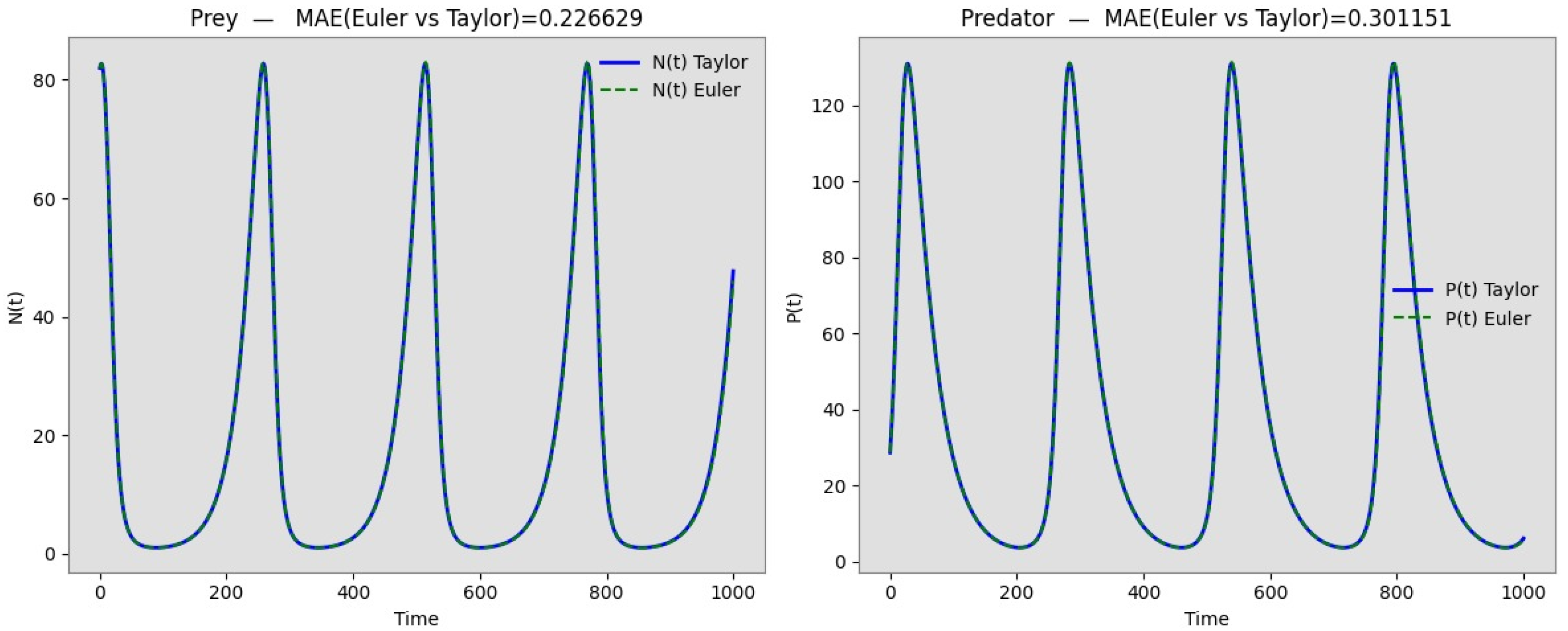
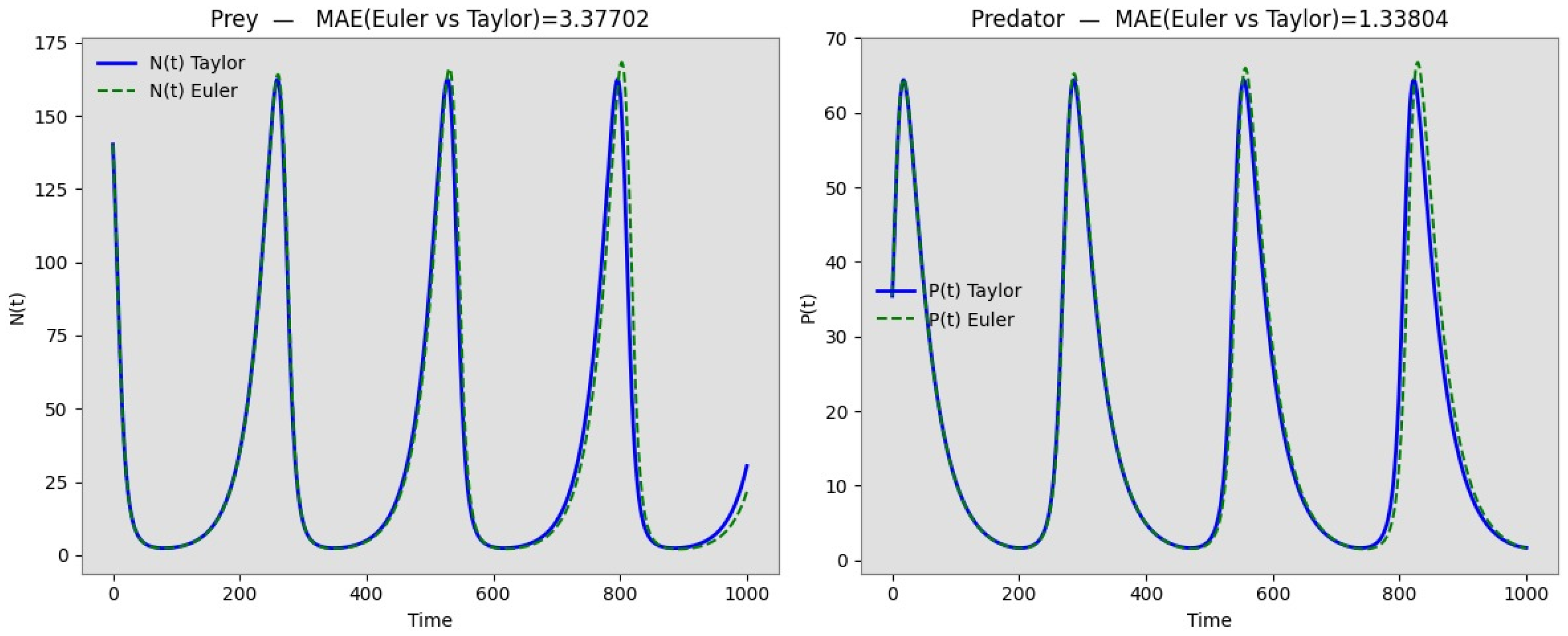
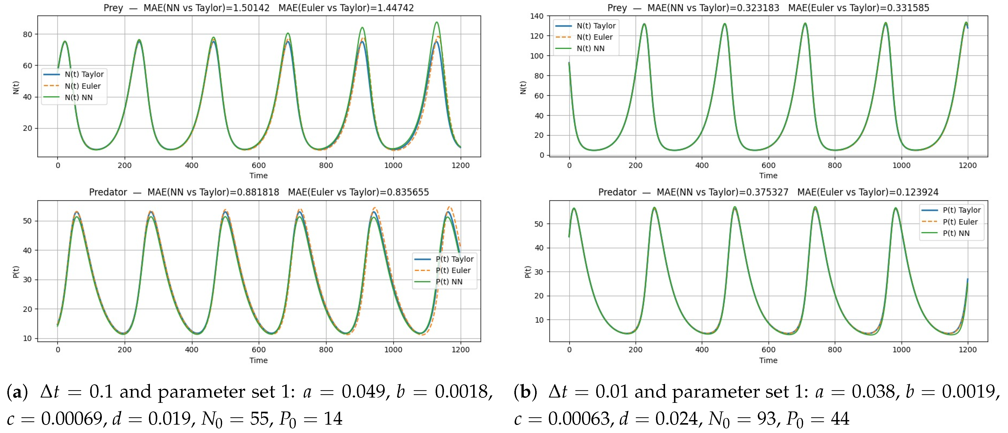
Figure 3 and Figure 4 show representative trajectories of the Lotka–Volterra system obtained using the explicit Euler method and the sixth-order Taylor method for $\Delta t=0.01$ and $\Delta t=0.1$, respectively. In both cases, the two numerical solutions are visually indistinguishable over the simulated time horizon, exhibiting nearly identical oscillation amplitudes, phases, long-term behavior, and minimal MAE.

In this regime, the local truncation error of the Euler method is sufficiently small that error accumulation remains negligible. Consequently, the residuals between Euler and Taylor6 solutions exhibit little structure, offering limited information for a neural model to exploit.

These results highlight an important practical observation: neural correction is unnecessary when the step size is already small enough for classical integrators to perform well. This motivates the focus of the proposed approach on moderate to large time steps, where Euler’s numerical errors become significant and structured, and where a learned correction can meaningfully improve long-term boundedness and accuracy.

To quantify the limited benefit of neural correction in the small time-step regime, we report the mean absolute error (MAE) averaged over 50 randomly sampled parameter combinations. The results in

Table 1. Average mean absolute error (MAE) for prey and predator populations in the small time-step regime, computed over 50 unseen parameter combinations. For $\Delta t=0.01$ and $\Delta t=0.1$, the explicit Euler method closely matches the high-order reference solution, resulting in low errors and limited potential for neural correction. Reported values correspond to mean ± standard deviation across all test cases.

$\mathbf{\Delta }\mathit{t}$	Average MAE Prey	Average MAE Predator
0.01	0.22 ± 0.25	0.34 ± 0.49
0.1	1.70 ± 2.11	2.76 ± 3.62

confirm that, for sufficiently small values of $\Delta t$, the explicit Euler method already achieves low error levels, leaving little room for improvement through learned correction.

7.2. Performance in the Intermediate Time Step Regime

We now evaluate the performance of the neural-corrected Euler method in the intermediate time-step regime, defined here by $\Delta t\in [0.5,1.1]$. This regime is particularly challenging: the time step is large enough for explicit Euler to accumulate significant phase and amplitude errors, yet not so large that the numerical solution immediately becomes unstable.

Table 2. Average MAE (mean ± standard deviation) over 50 unseen parameter combinations for explicit Euler and neural-corrected Euler in the intermediate time-step regime.

Method	$\mathbf{\Delta }\mathit{t}$	Average MAE Prey	Average MAE Predator
Euler	0.5	9.35 ± 6.61	13.21 ± 12.46
NN	0.5	2.51 ± 2.21	3.67 ± 3.64
Euler	0.8	12.83 ± 8.36	18.17 ± 15.95
NN	0.8	3.74 ± 2.91	7.22 ± 5.10
Euler	1	14.31 ± 8.72	20.09 ± 16.04
NN	1	4.68 ± 3.54	6.75 ± 6.47
Euler	1.1	14.66 ± 8.50	21.02 ± 16.41
NN	1.1	5.06 ± 3.35	10.02 ± 6.45

reports the mean absolute error (MAE) averaged over 50 independent parameter configurations, together with the corresponding standard deviation. Across all tested values of $\Delta t$, the neural corrector consistently reduces the error in both prey and predator populations. For $\Delta t=0.5$, the corrected method lowers the average MAE by approximately a factor of three relative to plain Euler, while also reducing error variability. As the time step increases to $\Delta t=0.8$ and $\Delta t=1.0$, the corrector continues to suppress the systematic error growth of Euler, achieving roughly a two- to three-fold reduction in MAE.

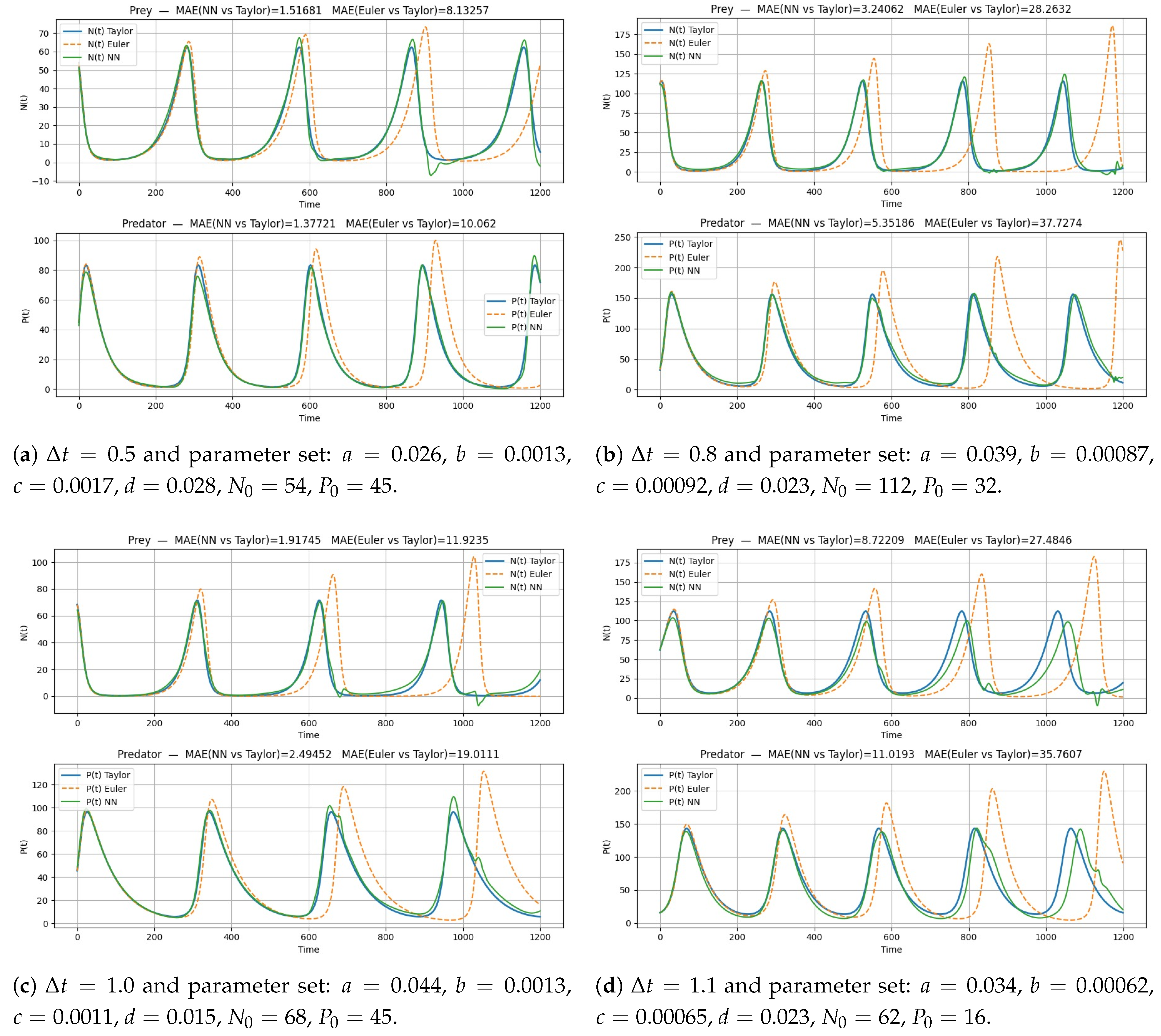
Even in the most demanding case $\Delta t=1.1$, where explicit Euler exhibits substantial error accumulation over long horizons, the neural-corrected scheme remains stable and achieves a significant reduction in both mean error and dispersion. This indicates that the network has learned a robust approximation of the dominant truncation error structure of Euler, rather than relying on fine-tuned corrections valid only for small step sizes.

The qualitative trajectory plots further support these findings. While plain Euler trajectories progressively drift in phase and amplitude as $\Delta t$ increases, the neural-corrected trajectories remain closely aligned with the Taylor order-6 reference over the entire integration interval. Taken together, these results demonstrate that the proposed neural corrector is particularly effective in the intermediate time-step regime, where classical low-order methods fail and high-order solvers may be computationally undesirable.

Figure 5 illustrates representative trajectories in the intermediate time-step regime for increasing values of $\Delta t$. In each case, the neural-corrected Euler trajectory is compared against both the raw Euler solution and the Taylor order-6 reference.

7.3. A Representative Case at $\Delta t=1.2$

Since the summary statistics in Table 2 are reported over 50 unseen parameter configurations for $\Delta t\le 1.1$, we additionally provide a representative unseen test case at $\Delta t=1.2$ to illustrate the behavior of the corrector in a larger-step regime.

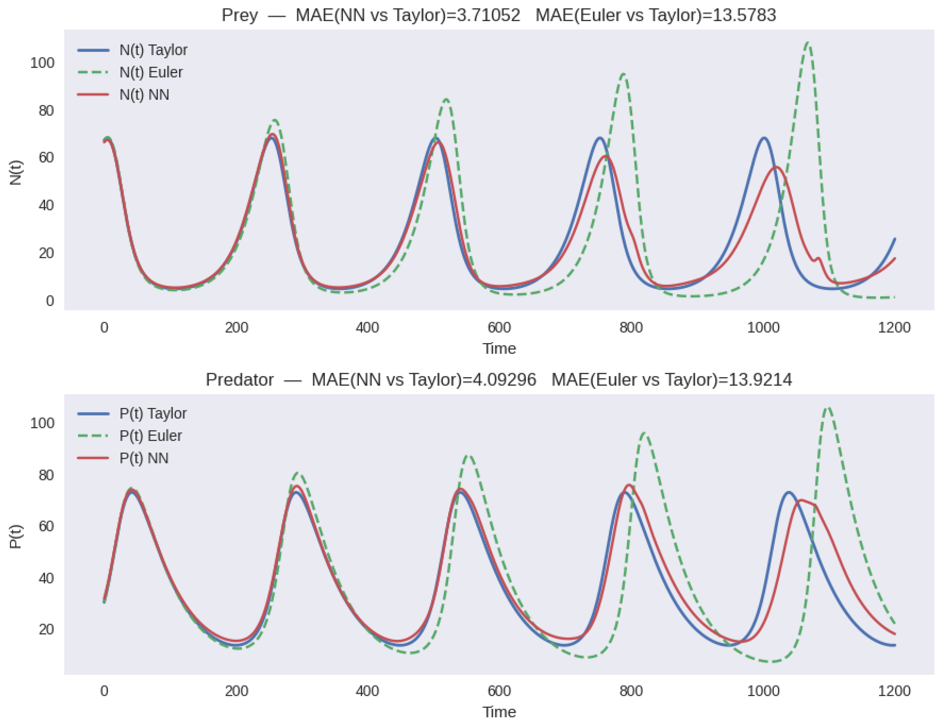
Figure 6 illustrates the trajectories obtained for this representative unseen configuration at $\Delta t=1.2$. The neural-corrected Euler solution remains significantly closer to the Taylor6 reference than the standard Euler approximation.

For completeness, we also examine the behavior of the neural corrector in the small time-step regime, where the explicit Euler method is already highly accurate. In this setting, little improvement is expected, and an effective corrector should preserve the base solution without introducing spurious dynamics.

As illustrated in Figure 7, for $\Delta t=0.1$ and $\Delta t=0.01$, the trajectories produced by explicit Euler, neural-corrected Euler, and the Taylor order-6 reference are nearly indistinguishable. This confirms that the learned model does not over-correct when the truncation error of Euler is already negligible, and acts as a stable identity mapping in regimes where correction is unnecessary.

Table 3. Representative test case at $\Delta t=1.2$ with parameters $a=0.0432487$, $b=0.00122765$, $c=0.000754945$, $d=0.0177671$, $N_0=67.0939$, $P_0=30.2070$.

Method	MAE Prey	MAE Predator
Euler	13.5783	13.9214
NN	3.7105	4.0930

Table 3. Representative test case at $\Delta t=1.2$ with parameters $a=0.0432487$, $b=0.00122765$, $c=0.000754945$, $d=0.0177671$, $N_0=67.0939$, $P_0=30.2070$.

Method	MAE Prey	MAE Predator
Euler	13.5783	13.9214
NN	3.7105	4.0930

7.4. Phase Portrait Preservation

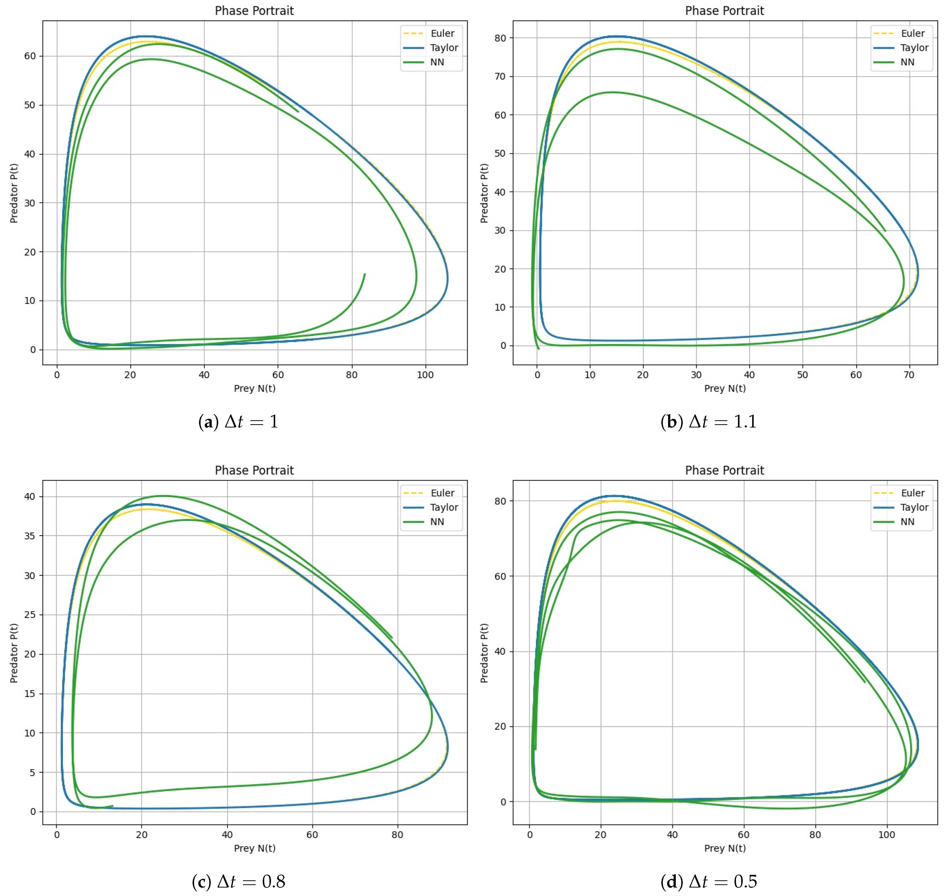
Beyond pointwise error metrics, the qualitative structure of the trajectories is crucial for oscillatory systems. Figure 8 compares phase portraits obtained with explicit Euler, neural-corrected Euler, and the Taylor6 reference.

The neural-corrected trajectories remain bounded and preserve the characteristic predator–prey phase portrait. However, they exhibit mild inward spiraling (artificial damping). This occurs because the network is trained to minimize MSE without any conservation constraint; it learns to “pull” the Euler trajectory back toward the reference, inadvertently introducing a slight dissipative bias. Despite this, the corrected scheme is qualitatively far superior to plain Euler in the intermediate $\Delta t$ regime (where Euler fails entirely). If exact invariant preservation is required, a physics-informed loss term or symplectic architecture could be added in future work. For the present purpose—stable, bounded long-term integration—the mild damping is acceptable.

7.5. Comparison with Runge–Kutta Methods

In this section, the performance of the proposed neural-corrected Euler scheme is evaluated against the classical fourth-order Runge–Kutta (RK4) method, as a practical high-order benchmark rather than as an exact reference. The objective of this comparison is not to outperform RK4 in general, but to extend the practical usability of Euler-type schemes in regimes where Euler alone fails and higher-order methods are undesirable.

All numerical experiments are performed using identical initial conditions and parameter sets. The RK4 method is applied with the same time-step size as the Euler-based methods in order to ensure a fair comparison. Accuracy is evaluated by comparing the resulting trajectories with respect to the RK4 solution.

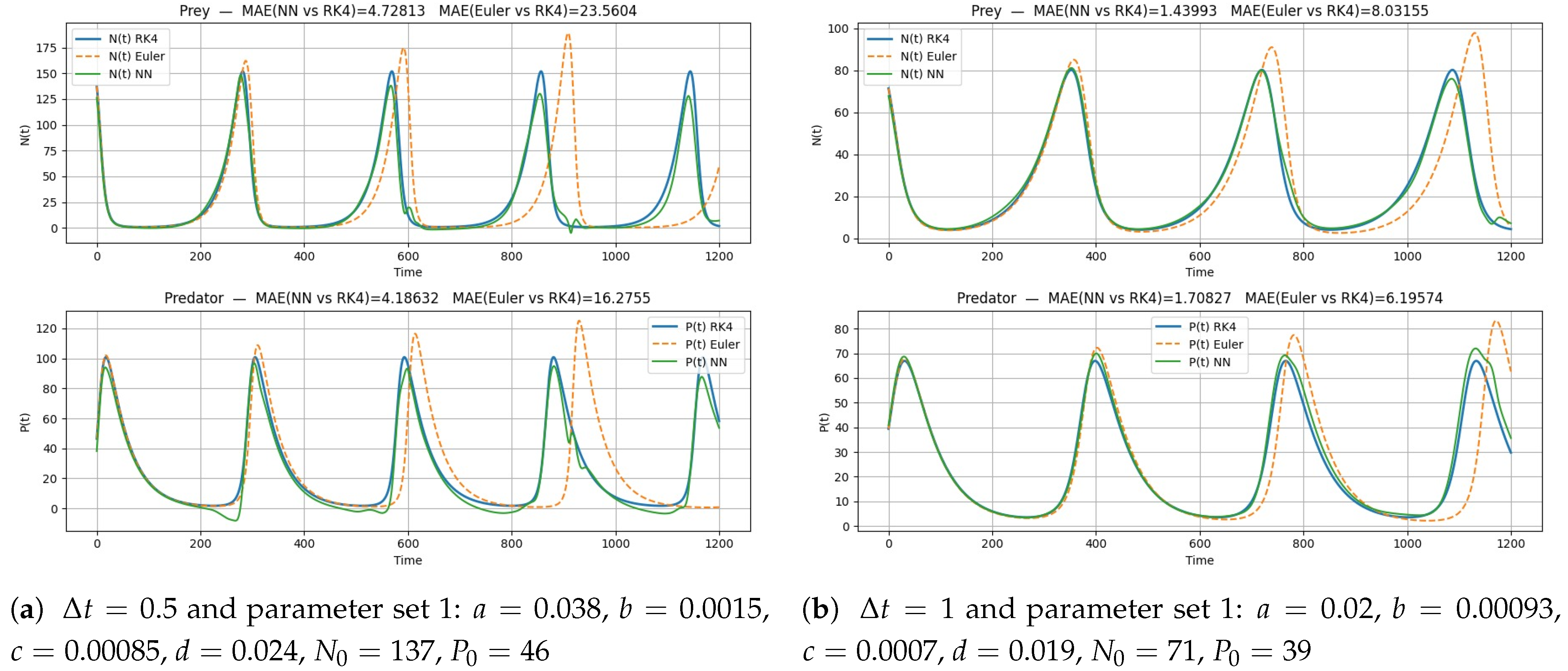
Figure 9 presents the system trajectories obtained using the standard Euler method, the neural-corrected Euler scheme, and the RK4 method for two representative time-step sizes, namely $\Delta t=1$ and $\Delta t=0.5$. These values correspond to regimes in which the explicit Euler method is known to suffer from significant numerical errors.

For both time-step sizes, the standard Euler method exhibits noticeable deviations from the trajectories produced by RK4, manifested as phase shifts and amplitude errors. In contrast, the neural-corrected Euler scheme substantially improves the numerical behavior, producing trajectories that remain qualitatively close to those generated by RK4 over the entire simulation interval. These results indicate that the learned correction effectively compensates for the dominant truncation error of the Euler method, particularly in the intermediate and large time-step regimes. It is important to emphasize that RK4 is used here solely as an additional benchmark for qualitative comparison, whereas the neural correction itself is trained with respect to the Taylor6 reference solution introduced earlier.

7.6. Computational Cost per Time Step

To complement the accuracy and stability analysis presented above, we evaluate the computational cost of the considered numerical schemes.

Table 4. Average wall-clock time per integration step for explicit Euler, classical RK4, and the neural-corrected Euler method, for different values of the time step $\Delta t$. The last two columns report the computational cost relative to explicit Euler.

$\mathbf{\Delta }\mathit{t}$	Euler (s/Step)	RK4 (s/Step)	NN (s/Step)	RK4/Euler	NN/Euler
0.5	1.72 × 10−5	1.11 × 10−4	1.16 × 10−3	6.47×	67.58×
0.8	1.45 × 10−5	4.93 × 10−5	8.81 × 10−4	3.41×	60.92×
1	8.96 × 10−6	5.21 × 10−5	8.78 × 10−4	5.82×	98.07×
1.1	4.62 × 10−6	2.92 × 10−5	4.56 × 10−4	6.32×	98.79×

reports the average wall-clock time per integration step for explicit Euler, classical fourth-order Runge–Kutta (RK4), and the proposed neural-corrected Euler method, measured for different values of the time step $\Delta t$. All benchmarks were performed on CPU using single-step inference without batching, in order to reflect a conservative and transparent implementation setting.

As expected, explicit Euler exhibits the lowest per-step computational cost, since it requires a single evaluation of the vector field and minimal arithmetic operations. The RK4 method incurs a higher cost, approximately 4–7× that of Euler, due to its four evaluations of the right-hand side per step.

The neural-corrected Euler method introduces a larger per-step overhead, typically between $60\times$ and $100\times$ that of explicit Euler. This increase is primarily due to neural network inference (feature construction, normalization, and evaluation of several fully connected layers). The per-step cost of the neural correction is almost independent of $\Delta t$, as expected for a fixed network architecture.

However, a direct per-step comparison with Euler is misleading in the regime where this method is intended to be used. For $\Delta t\ge 0.8$, the explicit Euler method does not produce bounded or qualitatively correct trajectories (see Table 2 and Figure 5). In this regime, a practitioner cannot simply use Euler with the same large $\Delta t˘$ as the simulation would be useless. The relevant alternatives are:

• Euler with a much smaller $\Delta t$ (e.g., $\Delta t=0.01$), which requires 80–100× more steps to cover the same time horizon, or
• Higher-order methods such as RK4, which remain stable but require more work per step.

Therefore, the efficiency of the neural-corrected Euler method must be evaluated in terms of total computational time to achieve a given accuracy, not per-step cost.

Table 5. Global mean absolute error versus total wall-clock time required to integrate the system up to a fixed final time T. While the neural-corrected Euler method incurs a higher per-step cost, the use of larger time steps results in a competitive trade-off between accuracy and total computational time.

Method	Total Time (s)	Global MAE
Euler	0.0578	1.58 $\times {10}^{-2}$
RK4	0.0142	5.87 $\times {10}^{-4}$
NN-Euler	0.0215	4.35 $\times {10}^{-3}$

shows this trade-off: for a fixed final time, the neural-corrected Euler (operating at $\Delta t=1.0$) achieves a global error that is two orders of magnitude smaller than Euler at $\Delta t=0.01$, while requiring only slightly more total time than RK4. Moreover, the neural correction is amortisable: once trained, it can be reused across many simulations (e.g., parameter sweeps, ensemble forecasts) with no additional training cost. In GPU-based or batched implementations, the relative overhead of neural inference drops significantly, making the method even more competitive.

Moreover, the reported overhead corresponds to a conservative implementation on CPU without batching or hardware acceleration. In scenarios involving more expensive vector field evaluations, higher-dimensional systems, or batched and GPU-based inference, the relative cost of the neural correction is expected to decrease, making the proposed method increasingly competitive.

These results highlight that per-step computational cost alone does not fully characterize the efficiency of a numerical integrator. When total integration time and achieved accuracy are jointly considered, the proposed neural-corrected Euler scheme offers a competitive alternative to classical methods.

8. Discussion

This work proposes a neural residual correction framework designed to enhance the explicit Euler method when applied to oscillatory dynamical systems, with a particular focus on the Lotka–Volterra equations. The results demonstrate that learning the local truncation error of Euler with respect to a high-order reference integrator can substantially improve both accuracy and long-term qualitative behavior, especially in regimes where classical low-order methods are known to fail [2].

8.1. Why the Neural Corrector Works

The effectiveness of the proposed approach stems from its formulation as a residual learning problem. Rather than approximating the solution of the differential system directly, the network is trained to predict the systematic error introduced by the explicit Euler update, in a manner analogous to residual learning strategies in deep networks [16]. This error exhibits strong and repeatable structure, depending on the system parameters, the current state, and the time-step size. By learning this structured truncation error, the network compensates for the dominant source of numerical inaccuracy while preserving the simplicity of the underlying integrator, consistent with recent approaches that learn corrections to numerical solvers [8,19].

Importantly, the correction operates locally at each time step, yet yields global improvements over long integration horizons. This indicates that the network captures not only instantaneous error patterns but also the mechanisms responsible for cumulative phase drift and amplitude inflation in Euler trajectories. The observed stabilization of long-term dynamics suggests that the learned correction implicitly mitigates the destabilizing energy injection typically associated with explicit Euler methods in conservative or near-conservative systems [18].

The mild inward spiraling observed in some phase portraits suggests a small dissipative bias introduced by the correction. While this effect slightly alters the invariant structure of the Lotka–Volterra system, it remains acceptable for applications where qualitative stability and boundedness are prioritized over exact conservation. Future work could mitigate this behavior by incorporating invariant-aware loss terms or soft conservation constraints during training.

8.2. Accuracy Across Time-Step Regimes

The numerical experiments highlight three distinct regimes. For small time steps, where explicit Euler already achieves high accuracy, the neural corrector behaves as a near-identity mapping, introducing no artificial distortion and preserving the reference dynamics. This property is crucial, as it confirms that the network does not over-correct when the base method is sufficient.

In the intermediate time-step regime, the proposed approach delivers its most significant benefits. Here, explicit Euler accumulates substantial phase and amplitude errors, while the neural-corrected scheme consistently reduces both the mean error and its variability across parameter configurations. This regime is particularly relevant in practice, as it represents a compromise between computational efficiency and long-term boundedness.

Although MAE is used as the primary quantitative metric throughout this study, the corrected trajectories also preserve the qualitative phase portrait structure of the Lotka–Volterra system, maintaining closed orbits and preventing the artificial spiraling behavior typically induced by explicit Euler at moderate and large time steps, in agreement with classical results on structure preservation in numerical integration [18].

8.3. Generalization and Robustness

A key result of this study is the strong generalization performance observed on unseen parameter sets.

Generalization was assessed by evaluating the neural-corrected scheme on parameter combinations not seen during training. Although the correction degrades gracefully outside the training range, performance remains stable as long as the qualitative dynamics of the system are preserved. The neural-corrected trajectories remain closely aligned with the high-order Taylor reference even for parameter combinations not encountered during training. This suggests that the network learns general properties of the Euler truncation error rather than memorizing specific trajectories, a behavior consistent with operator-learning frameworks for parametric dynamical systems [17,20]. Overfitting was mitigated through the use of moderate network depth, residual connections, normalization layers, and early stopping based on validation loss.

Furthermore, the corrector exhibits robustness across different dynamical regimes, including large-amplitude oscillations and parameter configurations far from equilibrium. Such behavior supports the interpretation of the model as a solver-informed correction mechanism, rather than a purely data-driven surrogate, aligning with the broader paradigm of theory-guided machine learning [21].

8.4. Computational Cost and Practical Regimes

One of the principal advantages of the explicit Euler method is its simplicity and extremely low computational cost. By introducing a neural residual corrector, the proposed framework necessarily increases the computational complexity of each integration step due to the additional neural-network evaluation. As shown in Table 4, the corrected method is significantly more expensive per step than the standard Euler scheme.

However, such a comparison is not entirely meaningful in isolation. In the intermediate and large time-step regimes considered in this work, the explicit Euler method often fails to produce bounded or qualitatively meaningful trajectories, regardless of its low per-step cost. Consequently, the relevant comparison is not with Euler itself, but with higher-order integrators capable of maintaining acceptable long-term behavior [2].

From this perspective, the proposed framework should not be interpreted as a universal replacement for optimized high-order solvers such as RK4, but rather as a proof-of-concept hybrid numerical–machine learning approach for learning truncation-error corrections. The additional computational cost represents a trade-off for improved qualitative accuracy and enhanced long-term boundedness in regimes where the explicit Euler method alone exhibits substantial numerical degradation.

An additional advantage of the framework lies in cost amortization. The neural corrector is trained offline and can subsequently be reused across multiple simulations with different initial conditions and parameter configurations. Moreover, the online correction stage requires only a forward pass through a relatively lightweight feedforward network, which is well suited for batching and hardware acceleration on modern GPUs.

Future work may further reduce the computational overhead through model compression, reduced architectures, adaptive correction strategies, or operator-learning approaches capable of handling varying time-step regimes within a single model.

8.5. Limitations and Future Work

Despite its effectiveness, the proposed approach has several limitations. First, the neural corrector is trained independently for each fixed time-step size $\Delta t$, requiring a separate model for each integration regime. While this design improves specialization and long-term boundedness in the targeted intermediate time-step regime, it limits practical flexibility in applications where adaptive time-stepping strategies are commonly employed. In particular, the current framework does not support dynamically varying time steps during integration, since the learned correction is specialized to the truncation-error structure associated with a specific $\Delta t$.

This limitation reflects an intentional design choice rather than a theoretical restriction. Preliminary experiments indicated that training a single network across substantially different time-step regimes led to degraded performance and reduced robustness, likely due to the distinct qualitative error structures exhibited by the explicit Euler method as $\Delta t$ varies. By training specialized models, the network can more effectively learn the dominant truncation-error operator associated with a given numerical regime. Nevertheless, extending the framework toward adaptive or continuous-in-$\Delta t$ correction models constitutes an important direction for future work. Possible approaches include incorporating $\Delta t$ directly as a continuous input feature, training multi-regime neural operators, or employing operator-learning architectures capable of generalizing across varying discretization scales [17,20]. Such extensions could significantly improve the practical applicability of neural-corrected integrators in realistic simulation settings.

Second, the present study focuses on a two-dimensional autonomous Lotka–Volterra system. Although the proposed residual correction framework is not inherently restricted to this particular model, the trained neural network itself should not be interpreted as universally transferable across arbitrary nonlinear systems. The learned correction depends strongly on the underlying vector field, the numerical stability properties of the system, and the specific truncation-error structure produced by the explicit Euler method. Consequently, different nonlinear systems would generally require retraining and, in some cases, modified feature representations or network architectures.

The framework could potentially be extended to higher-dimensional, stiff, chaotic, or multistable systems. In particular, systems exhibiting multistability may involve distinct attractors and qualitatively different dynamical regimes, which could alter the structure of the numerical truncation error. In such settings, trajectory-level information such as the initial conditions may help the neural corrector distinguish between different basins of attraction. However, multistable and chaotic dynamics may also introduce additional challenges related to regime switching, long-term stability preservation, and geometric structure conservation, which remain important directions for future investigation.

Additionally, rigorous theoretical guarantees concerning the long-term boundedness and qualitative behavior of neural-corrected integrators remain largely unexplored and warrant further mathematical investigation.

Nonetheless, the results presented here indicate that neural residual correction constitutes a promising and interpretable pathway for enhancing classical numerical solvers, combining the robustness of established integration schemes with the adaptability of modern machine learning techniques.

For chaotic systems such as the Lorenz system, the selection of the time-step size requires additional care. The step size should not be chosen merely to maximize computational speed, but rather to identify an intermediate regime in which the explicit Euler error is sufficiently structured to be learned while the uncorrected trajectory remains bounded and dynamically meaningful. Very small time steps leave little room for neural correction, whereas excessively large time steps may cause the Euler trajectory to leave the attractor or enter dynamically unrelated regions. In such systems, the corrected scheme should be assessed over finite prediction horizons and through qualitative or statistical quantities, such as attractor preservation, boundedness, invariant-measure statistics, or Lyapunov-type indicators, rather than by long-time pointwise agreement alone.

9. Conclusions

The main contribution of this work is not to provide a universally faster integrator, but to demonstrate that the local truncation error of the explicit Euler method can be learned and corrected in a numerically interpretable manner.

This work introduced a neural residual correction framework aimed at enhancing the explicit Euler method for the numerical integration of the Lotka–Volterra system under intermediate and large time-step sizes. By learning the local truncation error of Euler with respect to a high-order Taylor reference, the proposed approach significantly improves numerical accuracy while preserving the simplicity and interpretability of the base integrator.

Numerical experiments demonstrate that the neural-corrected Euler method consistently reduces phase and amplitude errors across a wide range of time steps and parameter configurations. In the intermediate regime, where explicit Euler is computationally attractive but numerically inaccurate, the proposed method achieves error reductions of up to an order of magnitude relative to the uncorrected scheme. Importantly, the corrector generalizes well to unseen parameter sets and remains stable over long integration horizons, indicating that it captures systematic properties of the Euler truncation error rather than overfitting to specific trajectories.

From a practical standpoint, the proposed framework offers a favorable trade-off between accuracy and computational cost. While the neural corrector introduces additional per-step overhead, it can remain computationally competitive with classical high-order solvers when larger time steps are employed. Moreover, the correction mechanism can be seamlessly integrated into existing Euler-based implementations, making it attractive for large-scale parameter studies and exploratory simulations of oscillatory systems.

Several directions for future work naturally arise from this study. Promising extensions include the development of time-step–adaptive correctors capable of operating across a continuous range of $\Delta t$ values within a single model, as well as the application of the approach to higher-dimensional, stiff, or externally forced dynamical systems. Finally, establishing formal stability and convergence guarantees for neural-corrected integrators remains an important open theoretical challenge.

Overall, these results demonstrate that the truncation error of the explicit Euler method exhibits a structured and learnable dependence on the system state, parameters, and time step. By exploiting this structure through neural residual correction, it is possible to substantially extend the practical range of Euler’s method while retaining its simplicity and low computational cost.