Performance Evaluation of a Single-Server Queueing System with Correlated Arrivals, Two-Tier Service Structure, Random Breakdowns and Phase-Type Repairs

Abstract

This paper analyzes a single-server queueing system with infinite capacity, where arrivals follow a Markovian arrival process and service and repair times are modeled by phase-type distributions. The service mechanism is two-tier: every customer undergoes a mandatory primary service, after which an optional secondary service is available upon request. When the system is empty, the server initiates a closedown process before taking successive multiple vacations; upon return, the server goes through a setup process before beginning service again. Service can be interrupted by random breakdowns in either mode, triggering a phase-type repair. Matrix-analytic methods are used for the steady-state analysis, yielding the stability condition, stationary probability vectors, busy period analysis and key performance measures. A cost analysis framework is also developed. Numerical experiments validate the analytical results and illustrate the practical applicability of the model.

1. Introduction

Queueing systems that integrate both the Markovian arrival process (MAP) and phase-type (PH) service distributions arise naturally in a wide range of modern service and communication environments. In telecommunications, for instance, call centers, data networks, and cellular base stations exhibit correlated and bursty traffic patterns that classical Poisson arrival models fail to capture adequately; MAP/PH models have therefore become the standard analytical framework for studying such systems. Beyond telecommunications, MAP/PH models have found broad application in cloud computing, where virtual machine requests arrive in correlated bursts and service times span multiple processing phases; in healthcare appointment systems, where patient inter-arrival times are correlated and treatments involve multiple sequential stages; and in financial transaction processing, where systems become overloaded when a large number of trades are executed at the same time, often during periods of high market volatility. Due to its wide-ranging applications, studying MAP/PH queueing systems carefully from a mathematical standpoint becomes crucial. This study not only deepens theoretical knowledge but also offers practical insights that aid in designing and optimizing real-world systems.

The analytical study of such systems has evolved considerably over the past several decades. Classical queueing theory models customer arrivals using the stationary Poisson process, which assumes a constant arrival rate, equidispersion (where the variance of arrivals equals their mean), and mutually independent inter-arrival times. Although convenient from a mathematical perspective, such conditions are unrealistic for modern network traffic, which is usually correlated and bursty. In recognition of the limitations of the Poisson process, Neuts [1] developed a significantly more descriptive stochastic framework, initially termed as the versatile arrival process (VAP) and later formalized as the MAP [2]. By incorporating burstiness, inter-arrival correlation, and state-dependent arrival behavior within a Markovian structure, the MAP overcomes many of the shortcomings of the Poisson process while retaining the analytical tractability necessary for mathematical analysis of complex traffic patterns. For further theoretical background and practical applications of the MAP in stochastic modelling, we direct the reader to [3,4,5,6].

A corresponding limitation exists in the modelling of the service process. Alongside the arrival process, the service time distribution plays an equally important role in determining the accuracy of queueing models. The exponential distribution has been used to represent a service time due to its memoryless property and mathematical simplicity. However, being a single-parameter distribution, it is unable to fully capture the variability and higher-order moments of real-world service processes. A PH distribution, defined as the distribution of time to absorption in a finite continuous-time Markov chain (CTMC), provides a practical and flexible alternative that effectively approximates general service time distributions. PH distributions are capable of simultaneously capturing both the mean and the higher-order moments of service times, while remaining within the analytically manageable framework of a Markov chain. Notable special cases within the PH family include the Erlang, hyper-exponential, and hypo-exponential distributions. Owing to these properties, PH distributions provide an analytically tractable representation of service processes in complex queueing systems, making them a natural and well-justified modelling choice for realistic queueing analysis. Further details regarding PH distributions may be found in [7,8,9].

Queueing models with server vacations have been applied to a broad range of application areas such as production systems, telecommunication networks, and service systems, particularly in contexts where server idle time can be effectively utilized for secondary tasks or energy conservation. Vacation policies are generally categorized into two types. Under a single vacation policy, the server resumes service immediately upon completing one vacation period, irrespective of the system’s current state. Conversely, under a multiple vacation policy, the server continues to take successive vacations until its return to find at least one customer awaiting service. In 1975, Levy and Yechiali [10] introduced the concept of server vacations and has since attracted considerable research attention. Comprehensive reviews of the early literature on vacation queueing systems were provided by Doshi [11], Takagi [12], and Tian and Zhang [13], while Ke et al. [14] offered a more concise survey of subsequent developments. Building on these foundations, numerous studies have extended vacation queueing models under a variety of operational assumptions and system configurations [15,16,17,18,19,20].

In practice, assuming perfectly reliable servers is rarely realistic, particularly in production and manufacturing systems, telecommunications infrastructure, and automated service environments, where servers are inherently susceptible to random failures. When a breakdown occurs during active service, the ongoing job is disrupted. The server then enters a repair phase, while new customers accumulate in the queue. Such interruptions inevitably increase congestion and degrade overall system performance. This practical reality has motivated considerable research interest in queueing systems subject to server breakdowns. An unreliable queueing model with a batch Markovian arrival process (BMAP) for arrivals, PH distributed service times, and N servers was analyzed in [21], where breakdown occurrences are governed by a MAP, repair times follow a PH distribution, and stationary performance characteristics are derived. Choudhary et al. [22] examined a MAP/PH/1 queue incorporating degradation in service rate alongside breakdowns, repairs, and phase-type vacations, analyzed using matrix-analytic methods. Dudin et al. [23] studied a MAP/PH single-server queue with server breakdowns and repairs, where both breakdown occurrences and arrivals follow independent MAPs and service and repair times follow PH distributions.

While much of the queueing literature has focused on systems offering a single mandatory service, many real-world service environments require the server to provide an additional supplemental service to a subset of customers upon completion of the primary service. Examples include hospital patients requiring post-treatment consultation, telecommunication users requesting additional data services, and manufacturing jobs requiring optional quality inspection after primary processing. The analytical study of such systems was pioneered by Madan [24], who analyzed the concept of second optional service in the context of an M/G/1 queue, examining both the time-dependent and steady-state behavior of the system using the supplementary variable technique. Building on this foundation, Medhi [25] extended the model by proposing an M/G/1 queue with a second optional channel, deriving explicit expressions for the mean queue length and mean waiting time. Wang [26] subsequently extended the model by incorporating server breakdowns, marking an important step toward more realistic system modelling. Chakravarthy [27] analyzed a queue with two types of service subject to vacations and optional secondary service, modelling arrivals via a MAP and service times via PH distributions. Vijaya Lakshmi and Girija Bhavani [28] analyzed a queueing model with second optional service and server breakdown, where service interruptions may occur during both the first essential service and the second optional service periods; they derived the stability condition and the stationary probability vector of the system.

Another practically important extension of queueing models concerns the inclusion of setup and closedown periods. In many real-world systems, the server requires a preparatory setup period before commencing service and a closedown period after serving the last customer before entering vacation or an idle state. Such operational features are common in manufacturing systems, batch processing environments, and communication networks. The concept of setup time in queueing systems was first introduced by Levy and Kleinrock [29] in the context of an M/M/1 queue, where the server requires an activation period upon the arrival of a new customer before service can commence. Building on this foundation, Bischof [30] and Gandhi et al. [31] further examined the impact of setup times on system performance under various queueing frameworks. Haghighi and Mishev [32] examined a transient $M^{\left[X\right]}/M^{(k,K)}/1$ queueing model with bulk arrivals following a compound Poisson process, batch service with minimum and maximum size constraints, exponentially distributed setup times, and customer reneging. Sun et al. [33] studied a gated service single vacation M/G/1 queue with setup and closedown periods under different customer arrival rates, deriving the stationary queue length distribution via the regeneration cycle method and establishing the stochastic decomposition of the queue length in steady state. Krishna Kumar et al. [34] analyzed a single server M/G/1 queue under Bernoulli vacation schedules with server setup and closedown periods, deriving the probability generating function of the queue length distribution using the imbedded Markov chain technique, along with the Laplace–Stieltjes transform of the waiting time distribution and corresponding mean performance measures.

Despite the extensive body of literature on MAP/PH queueing systems, server vacations, optional supplementary service, and server breakdowns, these features have largely been studied in isolation or in limited combinations. To the best of our knowledge, no existing study has simultaneously incorporated all of the following features within a single unified queueing framework: MAP for correlated and bursty arrivals, PH distributions for both essential and optional service times, an optional supplementary service available to a subset of customers upon completion of essential service, server breakdowns with PH distributed repair times occurring during both essential and optional service periods, a closedown period initiated after serving the last customer, a setup period required before the server resumes service, and a multiple vacation policy adopted by the server during idle periods. The absence of such a comprehensive model represents a significant gap in the queueing literature, particularly given the practical relevance of these features in modern telecommunication networks, cloud computing environments, health care systems, and manufacturing systems. Addressing this gap is therefore both theoretically motivated and practically justified, forming the primary impetus for the present study.

1.1. Motivation

Modern cloud computing platforms and data centers operate under highly unpredictable conditions. Incoming workloads rarely follow simple, independent patterns; instead, requests tend to arrive in bursts, exhibit correlations, and fluctuate based on user behavior, application interactions, and network dynamics. Under these conditions, the classical Poisson arrival model falls short, and a more flexible framework such as the MAP becomes essential for realistically capturing how tasks enter the system.

Not all arriving tasks share the same service requirements. Every customer first receives a mandatory primary service covering core operations such as request handling and response generation. Following this, certain tasks may require additional processing such as data logging, encryption, or verification which is offered as an optional secondary service on a probabilistic basis. This two-stage service structure reflects the natural heterogeneity of real-world workloads.

Server reliability is another practical concern. Hardware failures, software faults, and network disruptions can interrupt service unexpectedly, and recovery is rarely immediate. Since repair processes typically unfold in multiple stages, PH distributions are used to model repair times, allowing for more realistic performance predictions during periods of disruption.

Energy efficiency is equally important in large-scale systems. Keeping servers fully active during idle periods is wasteful, so when the system empties, the server undergoes a closedown process before entering a vacation state. When new tasks eventually arrive, a setup phase is required before full service resumes. These transitions, though brief, meaningfully affect system responsiveness and cost.

By integrating correlated arrivals, heterogeneous service requirements, random breakdowns with multi-stage repairs, and energy-aware operational control, the proposed model provides a realistic and comprehensive analytical tool for evaluating modern service infrastructures.

1.2. Novelty and Contribution

The proposed model advances existing queueing literature by integrating operational dynamics, reliability effects, and energy-aware control mechanisms in a mutually dependent manner, rather than treating them as isolated features. To clearly demonstrate the novelty of the proposed model,

Table 1. Comparison of the proposed model with existing literature.

Reference	Arrival Process	Essential Service	Optional Service	Breakdown	Repair Dist.	Closedown	Vacation	Setup
Madan [24]	M	G	✓	✗	–	✗	✗	✗
Medhi [25]	M	G	✓	✗	–	✗	✗	✗
Wang [26]	M	G	✓	✓	G	✗	✗	✗
Levy & Kleinrock [29]	M	G	✗	✗	–	✗	✓	✓
Chakravarthy [27]	MAP	PH	✓	✗	–	✗	✓	✗
Dudin et al. [23]	MAP	PH	✗	✓	PH	✗	✗	✗
Proposed model	MAP	PH	✓	✓	PH	✓	✓	✓

✓: Feature present; ✗: Feature absent; –: Not applicable. M: Poisson; G: General; MAP: Markovian Arrival Process; BMAP: Batch MAP; PH: Phase-Type.

presents a systematic feature-by-feature comparison with closely related works in the literature. It is evident that while individual features such as optional service, server breakdowns with repairs, vacation policies, and closedown and setup periods have been studied separately or in limited combinations, no existing work simultaneously incorporates all of these features within a unified MAP/PH framework.

Specifically, the main contributions of this work are as follows:

• Heterogeneous and multi-stage service modeling: The model incorporates an optional supplementary service available to a subset of customers upon completion of the primary essential service, with both service stages represented by PH distributions. This enhances modeling generality and permits the approximation of a wide class of practical service time distributions beyond the exponential assumption.
• Server reliability modeling: Server interruptions may occur randomly during both the essential and optional service periods, with repair times modeled using PH distributions. This captures the multi-stage nature of real-world recovery processes and allows for more accurate performance predictions during periods of disruption.
• Energy-aware operational control: The model incorporates a non-instantaneous closedown period initiated upon system emptying, followed by repeated multiple vacation periods, and a setup phase required before the server resumes service. These features enable the evaluation of critical trade-offs between system performance and energy efficiency, which are highly relevant in contemporary large-scale service infrastructures.
• Mathematical modeling and performance analysis: The system is modeled as a CTMC with an explicitly structured state space, yielding a block-structured infinitesimal generator matrix. Matrix-analytic methods are employed to derive the stability condition, stationary probability distribution, busy period analysis, and key performance measures, providing a unified analytical framework for studying complex queueing systems.

Overall, the proposed framework offers a novel queueing model that simultaneously captures optional service, server breakdowns with PH-distributed repairs, and energy-aware server control through closedown, vacation, and setup mechanisms. To the best of the authors’ knowledge, this combination has not been previously studied in the literature. The busy period analysis further distinguishes this work, providing additional theoretical depth and practical utility for the design and evaluation of complex service systems.

1.3. Organization of the Paper

The remainder of this paper is organized as follows. Section 2 presents the model description, including the mathematical formulation, state space construction, and the block-structured infinitesimal generator matrix, along with the stability condition of the system. The steady-state probability vector is derived in Section 3 using matrix-analytic methods. Section 4 is devoted to the analysis of the busy period. The system performance measures and the total average cost function are evaluated in Section 5. Section 6 examines several special cases of the proposed model, including the classical Poisson arrival with exponential service as a limiting case. Numerical illustrations, presented both tabularly and graphically, are provided in Section 7 to validate the analytical results and demonstrate the effect of system parameters on performance measures. Finally, Section 8 concludes the paper with a summary of findings and directions for future research.

Notations

Throughout this paper, the following standard mathematical conventions are observed. The symbols ⊗ and ⊕ denote the Kronecker product and Kronecker sum of matrices, respectively. For any positive integer m, the symbol ${\mathit{e}}_m$ denotes a column vector of ones of dimension m, while I denotes an identity matrix whose order is determined by the context in which it appears. All other notation is introduced at the point of first use.

2. Model Description

This work considers a single-server queueing system with infinite waiting capacity, operating under a first-come, first-served discipline. The model incorporates two service modes, multiple vacations, closedown and setup mechanisms, and random server failures with phase-type repairs. The system dynamics are described as follows.

The flow of incoming customers is modelled by means of a MAP, wherein arrival events are embedded within a CTMC that evolves over a finite state space of dimension $m.$ Two square matrices $C_0$ and $C_1$ of order m provide a complete characterization of the process. The matrix $C_0$ governs non-arrival transitions and $C_1$ governs transitions that emit an arrival, such that the generator $C=C_0+C_1$ is irreducible and $C_0$ has negative diagonal entries and non-negative off-diagonals, while $C_1$ is non-negative. The fundamental arrival rate of the process is recovered as $\lambda =\mathit{\pi }{C}_1\mathit{e}$, where $\mathit{\pi }$ satisfies the following conditions:

$$\mathit{\pi }\mathit{C}=\mathbf{0}\mathrm{and}\mathit{\pi }\mathit{e}=\mathbf{1},$$

(1)

representing the stationary distribution of the underlying Markov chain.

Once service begins, every customer first undergoes Normal Service (NS) without exception, delivered in the order of arrival. The NS duration follows a PH distribution parameterized by $(\alpha ,T)$ of order $d_n^s$, where $\alpha$ represents the probability vector governing which internal phase the service begins in and satisfies $\alpha \mathit{e}=1$, and T is the sub-generator matrix governing transitions between service phases with strictly negative diagonals and non-negative off-diagonals. The rate at which customers complete NS is captured by the vector $T_0=-T\mathit{e}$. Consequently, the mean NS duration is ${\mu }_n^{-1}=\alpha {(-T)}^{-1}\mathit{e}$, offering a convenient closed-form expression for the average time spent in primary service (NS).

Upon completing NS, a customer may either request an additional Optional Service (OS) with probability a, or leave the system immediately with probability $b=1-a$, depending on individual need. The OS duration is again modeled by a PH distribution, now characterized by $({\alpha }^{\prime },T^{\prime })$ of order $d_o^s$, where ${\alpha }^{\prime }$ gives the initial phase probabilities and $T^{\prime }$ acts as the sub-generator for phase transitions inside this stage. The exit rate from OS equals $T_0^{\prime }=-T^{\prime }\mathit{e}$, leading to a mean optional service time of ${\mu }_o^{-1}={\alpha }^{\prime }{(-T^{\prime })}^{-1}\mathit{e}$.

When the last waiting customer departs the system after service completion, the server initiates a closedown process, during which necessary shutdown tasks are performed before the server can proceed to vacation. The closedown duration is assumed to follow an exponential distribution with rate $\zeta$. Following the completion of the closedown process, the server enters a vacation period. If no customers are found waiting upon the server’s return, it does not remain idle. Instead, another vacation is initiated, and this cycle continues until demand re-emerges. This repeated mechanism follows the classical multiple vacation policy. Each vacation duration is exponentially distributed with rate $\nu$. Upon returning from vacation to find customers waiting, the server does not resume service immediately. A setup process is first carried out, during which the server prepares and reinitializes itself for active operation. This setup phase is governed by an exponential distribution with rate $\xi$, after which the server begins service to the waiting customers.

During either NS or OS, the server is subject to random failures that interrupt the ongoing service. Breakdowns occur at exponential rates ${\upsilon }_n$ and ${\upsilon }_o$ during NS and OS, respectively, and upon failure, the server immediately enters a repair process while the interrupted customer remains in the system awaiting restoration of service. The repair duration is modeled using PH distributions, represented by $(\beta ,E)$ and $({\beta }^{\prime },E^{\prime })$ of dimensions $d_n^r$ and $d_o^r$ for failures occuring during NS and OS, respectively, where $E_0=-E\mathit{e}$ and $E_0^{\prime }=-E^{\prime }\mathit{e}.$ The mean repair times are thus given by ${\sigma }_n^{-1}=\beta (-E^{-1})\mathit{e}$ and ${\sigma }_o^{-1}={\beta }^{\prime }(-{E^{\prime }}^{-1})\mathit{e}.$

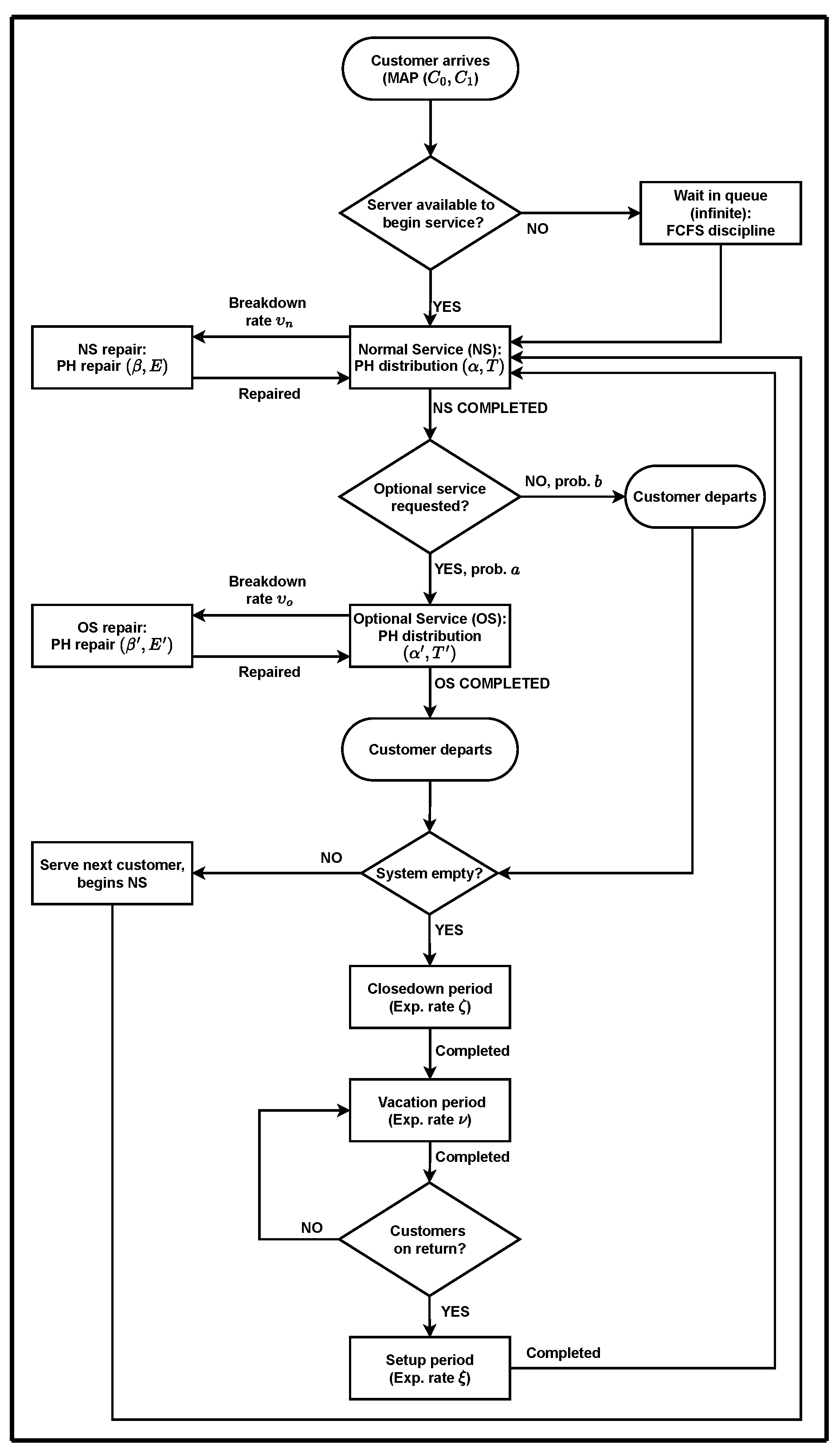
The overall flow of the proposed queueing system, is illustrated in Figure 1.

Markov Process

To formally characterize the time evolution of the system, a set of continuous-time random variables is introduced, each tracking a distinct aspect of the system’s state at any given moment $t\ge 0$:

• $J_1\left(t\right)$: the total number of customers present in the system;
• $J_2\left(t\right)$: the operational mode of the server, where

  $$\begin{array}{c}\hfill J_2\left(t\right)=\left\{\begin{array}{cc}0,\hfill & \mathrm{if}\mathrm{server}\mathrm{is}\mathrm{engaged}\mathrm{in}\mathrm{NS},\hfill \\ 1,\hfill & \mathrm{if}\mathrm{server}\mathrm{is}\mathrm{engaged}\mathrm{in}\mathrm{OS},\hfill \\ 2,\hfill & \mathrm{if}\mathrm{server}\mathrm{is}\mathrm{under}\mathrm{repair}\mathrm{following}\mathrm{a}\mathrm{breakdown}\mathrm{during}\mathrm{NS},\hfill \\ 3,\hfill & \mathrm{if}\mathrm{server}\mathrm{is}\mathrm{under}\mathrm{repair}\mathrm{following}\mathrm{a}\mathrm{breakdown}\mathrm{during}\mathrm{OS},\hfill \\ 4,\hfill & \mathrm{if}\mathrm{server}\mathrm{is}\mathrm{in}\mathrm{the}\mathrm{closedown}\mathrm{state},\hfill \\ 5,\hfill & \mathrm{if}\mathrm{server}\mathrm{is}\mathrm{on}\mathrm{vacantion},\hfill \\ 6,\hfill & \mathrm{if}\mathrm{server}\mathrm{is}\mathrm{in}\mathrm{the}\mathrm{setup}\mathrm{state}.\hfill \end{array}\right.\end{array}$$
• $J_3\left(t\right)$: the phase of server providing NS;
• $J_4\left(t\right)$: the phase of server providing OS;
• $J_5\left(t\right)$: the phase of repair when a breakdown occurs during the NS;
• $J_6\left(t\right)$: the phase of repair when a breakdown occurs during the OS;
• $J_7\left(t\right)$: the state of the fundamental process of MAP.

The joint process ${\{J_1\left(t\right),J_2\left(t\right),J_3\left(t\right),J_4\left(t\right),J_5\left(t\right),J_6\left(t\right),J_7\left(t\right)\}}_{t\ge 0}$ constitutes a CTMC whose transition structure naturally exhibits the form of a Quasi-Birth-Death (QBD) process. In this context, $J_1\left(t\right)$, representing the number of customers in the system, serves as the level of the process, a non-negative integer that indexes the repeating block structure of the infinitesimal generator matrix while the remaining variables $J_2\left(t\right),\dots ,J_7\left(t\right)$ collectively define the phase, capturing the internal operational state at each level. The complete state space of this CTMC is given by

$$\Omega ={\displaystyle \bigcup _{j_1=0}^{\infty }}{l}^{\ast }\left(j_1\right),$$

(2)

where the boundary level $j_1=0$ captures the states in which the system is empty, with the server either in closedown or vacation mode:

$$\begin{array}{c}\hfill l^{\ast }\left(0\right)=\{(0,j_2,j_7),4\le j_2\le 5,1\le j_7\le m\},\end{array}$$

and for $j_1\ge 1,$ each level encompasses all possible server status modes and their associated phase combinations:

$$\begin{array}{cc}\hfill l^{\ast }\left(j_1\right)=& \{(j_1,0,j_3,j_7):1\le j_3\le d_n^s,1\le j_7\le m\}\hfill \\ \hfill & \cup \{(j_1,1,j_4,j_7):1\le j_4\le d_o^s,1\le j_7\le m\}\hfill \\ \hfill & \cup \{(j_1,2,j_5,j_7):1\le j_5\le d_n^r,1\le j_7\le m\}\hfill \\ \hfill & \cup \{(j_1,3,j_6,j_7):1\le j_6\le d_o^r,1\le j_7\le m\}\hfill \\ \hfill & \cup \{(j_1,4,j_7):1\le j_7\le m\}\hfill \\ \hfill & \cup \{(j_1,5,j_7):1\le j_7\le m\}\hfill \\ \hfill & \cup \{(j_1,6,j_7):1\le j_7\le m\}.\hfill \end{array}$$

At the boundary level $j_1=0$, only the closedown ($J_2\left(t\right)=4$) and vacation ($J_2\left(t\right)=5$) modes are active, each combined with the m states of the MAP process, yielding a total of $2m$ states. At each non-boundary level $j_1\ge 1$, all the seven modes of server are present: the NS phase ($d_n^s$ states), the OS phase ($d_o^s$ states), repair following breakdown during NS ($d_n^r$ states), repair following breakdown during OS ($d_o^r$ states), the closedown, vacation, and setup modes are the contributing 3 states, each combined with the m states of the MAP process. This gives a total of $(d_n^s+d_o^s+d_n^r+d_o^r+3)m$ states at each level $j_1\ge 1$.

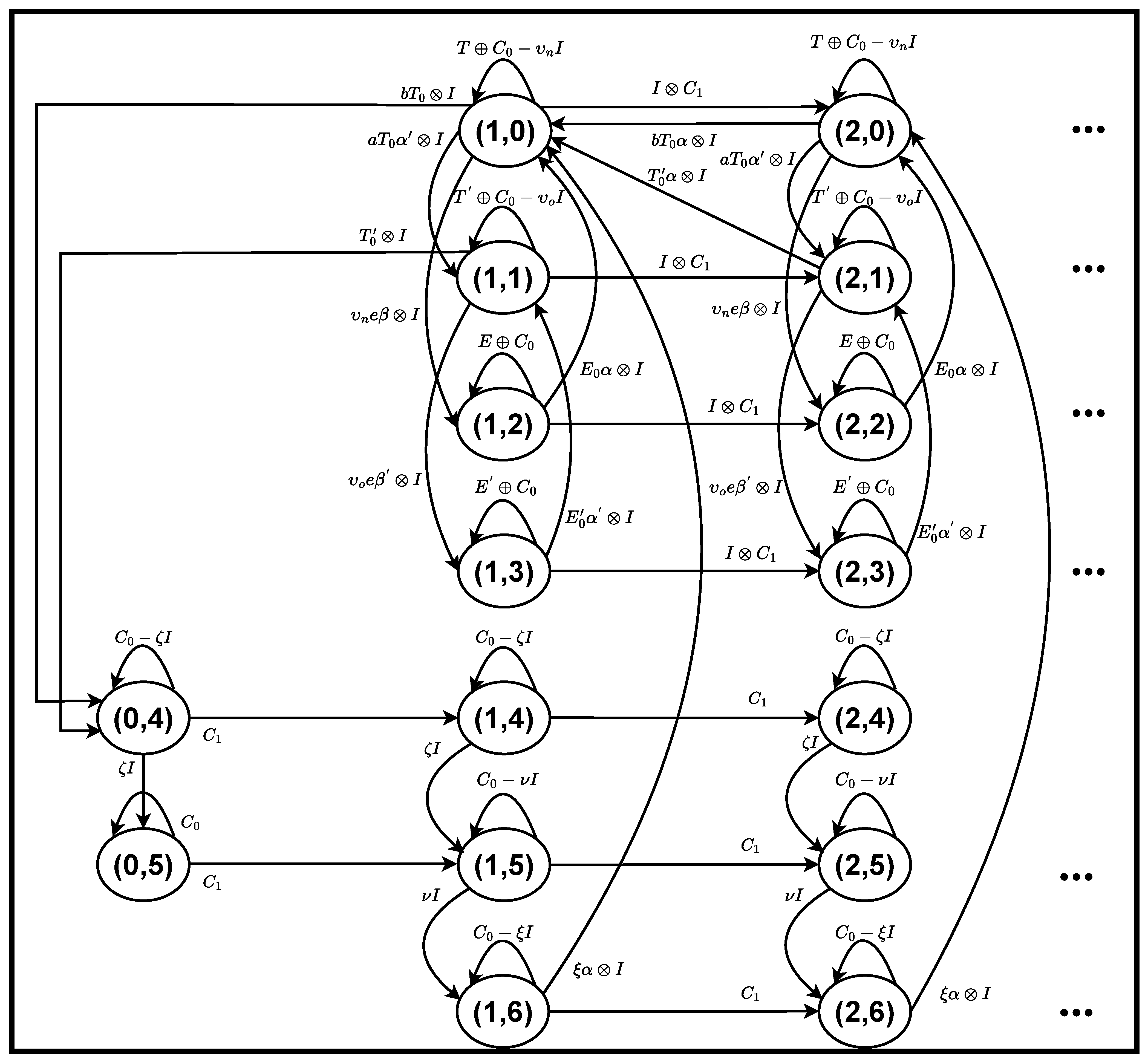
A pictorial representation of the state transitions governing the system dynamics is presented in Figure 2.

Lemma 1.

The infinitesimal generator matrix ${\mathbf{Q}}^{\ast }$ for the underlying process has a block-tridiagonal form:

$${\mathbf{Q}}^{\ast }=\left[\begin{array}{cccccc}{A}_{00}& A_{01}& & & & \\ A_{10}& M_1& M_0& & & \\ & M_2& M_1& M_0& & \\ & & M_2& M_1& M_0& \\ & & & \ddots & \ddots & \ddots \end{array}\right].$$

(3)

In other words, generator matrix consists of boundary blocks $A_{00}$, $A_{01}$, and $A_{10}$ that describe the transitions at level 0 and between levels 0 and 1, while the repeating blocks $M_0$, $M_1$, and $M_2$ capture the consistent transition patterns for all higher levels $j_1\ge 1$.

Proof. 

The block structure of ${\mathbf{Q}}^{\ast }$ follows directly from the state space construction and the operational dynamics of the proposed model. We establish the form of each block matrix by systematically identifying all feasible transitions between system states.

Boundary Blocks:

• $A_{00}$: The block $A_{00}$ of dimension $2m\times 2m$ governs transitions within level $j_1=0$, where the system is empty and the server is either in the closedown state or the vacation state. When the server is in the closedown state, it transitions to the vacation state at rate $\zeta$, while the MAP phase continues to evolve according to $C_0$, capturing non-arrival transitions. Consequently:

  $$A_{00}=\left[\begin{array}{cc}{C}_0-\zeta I_m& \zeta I_m\\ 0_m& C_0\end{array}\right].$$

  (4)
  Diagonal blocks $C_0-\zeta I_m$ and $C_0$ represent the self-transition rates in the closedown and vacation substates, respectively, and the off-diagonal block $\zeta I_m$ represents the transition from closedown to vacation at rate $\zeta$.
• $A_{01}$: The block $A_{01}$ of dimension $2m\times (d_n^s+d_o^s+d_n^r+d_o^r+3)m$ captures transitions from level 0 to level 1, which occur exclusively due to customer arrivals governed by the MAP transition matrix $C_1$. When a customer arrives while the server is in the closedown state or on vacation, no ongoing process is interrupted, the arriving customer simply joins the queue, causing the system to move from level 0 to level 1, while the server continues its current closedown or vacation process uninterrupted:

  $$A_{01}=\left[\begin{array}{ccccccc}{0}_{m,d_n^{s}m}& 0_{m,d_o^{s}m}& 0_{m,d_n^{r}m}& 0_{m,d_o^{r}m}& C_1& 0_m& 0_m\\ 0_{m,d_n^{s}m}& 0_{m,d_o^{s}m}& 0_{m,d_n^{r}m}& 0_{m,d_o^{r}m}& 0_m& C_1& 0_m\end{array}\right].$$

  (5)
  Nonzero entries $C_1$ appear in the columns corresponding to the closedown and vacation substates at level 1, reflecting that the server remains in its current operational state following the arrival.
• $A_{10}$: The block $A_{10}$ of dimension $(d_n^s+d_o^s+d_n^r+d_o^r+3)m\times 2m$ governs transitions from level 1 to level 0, which occur when the last customer in the system departs, leaving the system empty. Specifically, upon completion of normal service, a customer departs without requiring optional service with probability b, directly leaving the system and contributing the term $b{T}_0\otimes I_m$ to the transition structure. Upon completion of optional service, the customer has received both stages of service and departs, contributing $T_0^{\prime }\otimes I_m$. In both cases, the departure of the last customer causes the system level to drop from 1 to 0, triggering the closedown process. All other substates at level 1, including repair, closedown, vacation, and setup, do not generate customer departures and therefore contribute zero blocks:

  $$A_{10}=\left[\begin{array}{cc}b{T}_0\otimes I_m& 0_{d_n^{s}m,m}\\ T_0^{\prime }\otimes I_m& 0_{d_o^{s}m,m}\\ 0_{d_n^{r}m,m}& 0_{d_n^{r}m,m}\\ 0_{d_o^{r}m,m}& 0_{d_o^{r}m,m}\\ 0_m& 0_m\\ 0_m& 0_m\\ 0_m& 0_m\end{array}\right].$$

  (6)

Level-independent Blocks for $j_1\ge 1$:

• Level-Increment Block $M_0$: The block $M_0$ of dimension $(d_n^s+d_o^s+d_n^r+d_o^r+3)m\times (d_n^s+d_o^s+d_n^r+d_o^r+3)m$ represents transitions from level $j_1$ to level $j_1+1$, corresponding to new customer arrivals. Arrivals can occur independently of the server’s current state, whether it is serving, under repair, on vacation, in setup, or in closedown. This results in a block-diagonal structure, where each diagonal block is formed as the Kronecker product of the arrival matrix $C_1$ and the identity matrix of appropriate dimension:

  $$M_0=\left[\begin{array}{ccccccc}{I}_{d_n^s}\otimes C_1& 0& 0& 0& 0& 0& 0\\ 0& I_{d_o^s}\otimes C_1& 0& 0& 0& 0& 0\\ 0& 0& I_{d_n^r}\otimes C_1& 0& 0& 0& 0\\ 0& 0& 0& I_{d_o^r}\otimes C_1& 0& 0& 0\\ 0& 0& 0& 0& C_1& 0& 0\\ 0& 0& 0& 0& 0& C_1& 0\\ 0& 0& 0& 0& 0& 0& C_1\end{array}\right].$$

  (7)
  The seven block rows correspond to the substates of normal service, optional service, normal repair, optional repair, closedown, vacation, and setup, respectively.
• Self-Transition Block $M_1$: The block $M_1$ of dimension $(d_n^s+d_o^s+d_n^r+d_o^r+3)m\times (d_n^s+d_o^s+d_n^r+d_o^r+3)m$ captures all transitions within the same level $j_1\ge 1$. These include:

  -

  Phase transitions with normal service governed by $T\oplus C_0$, with breakdown occurring at rate ${\upsilon }_n$ and optional service being initiated with probability a upon normal service completion via $a{T}_0{\alpha }^{\prime }\otimes I_m$;

  -

  Phase transitions with optional service governed by $T^{\prime }\oplus C_0$, with breakdown occurring at rate ${\upsilon }_o$;

  -

  Repair phase transitions for normal and optional service breakdowns, governed by $E\oplus C_0$ and $E^{\prime }\oplus C_0$, respectively, with repair completions returning the server to the corresponding service phase via $E_0\alpha \otimes I_m$ and $E_0^{\prime }{\alpha }^{\prime }\otimes I_m$;

  -

  Closedown transitions at rate $\zeta$ to vacation, and vacation transitions at rate $\nu$ to setup;

  -

  Setup completion at rate $\xi$, triggering the start of normal service via $\xi \alpha \otimes I_m$.

  These transitions collectively yield:

  $$M_1=\left[\begin{array}{ccccccc}T\oplus C_0-{\upsilon }_n{I}_{m{d}_n^s}& a{T}_0{\alpha }^{\prime }\otimes I_m& {\upsilon }_n{e}_{d_n^s}\beta \otimes I_m& 0& 0& 0& 0\\ 0& T^{\prime }\oplus C_0-{\upsilon }_o{I}_{m{d}_o^s}& 0& {\upsilon }_o{e}_{d_o^s}{\beta }^{\prime }\otimes I_m& 0& 0& 0\\ E_0\alpha \otimes I_m& 0& E\oplus C_0& 0& 0& 0& 0\\ 0& E_0^{\prime }{\alpha }^{\prime }\otimes I_m& 0& E^{\prime }\oplus C_0& 0& 0& 0\\ 0& 0& 0& 0& C_0-\zeta I_m& \zeta I_m& 0\\ 0& 0& 0& 0& 0& C_0-\nu I_m& \nu I_m\\ \xi \alpha \otimes I_m& 0& 0& 0& 0& 0& C_0-\xi I_m\end{array}\right].$$

  (8)
• Level-Decrement Block $M_2$: The block $M_2$ of dimension $(d_n^s+d_o^s+d_n^r+d_o^r+3)m\times (d_n^s+d_o^s+d_n^r+d_o^r+3)m$ represents transitions from level $j_1$ to level $j_1-1$, corresponding to service completions that result in a customer departure. Departures can only occur upon the completion of normal service (with probability b, the customer does not require optional service) or upon the completion of optional service. These completions are captured by $b{T}_0\alpha \otimes I_m$ and $T_0^{\prime }\alpha \otimes I_m$, respectively:

  $$M_2=\left[\begin{array}{ccccccc}b{T}_0\alpha \otimes I_m& 0_{d_n^{s}m,d_o^{s}m}& 0_{d_n^{s}m,d_n^{r}m}& 0_{d_n^{s}m,d_o^{r}m}& 0_{d_n^{s}m,m}& 0_{d_n^{s}m,m}& 0_{d_n^{s}m,m}\\ T_0^{\prime }\alpha \otimes I_m& 0_{d_o^{s}m,d_o^{s}m}& 0_{d_o^{s}m,d_n^{r}m}& 0_{d_o^{s}m,d_o^{r}m}& 0_{d_o^{s}m,m}& 0_{d_o^{s}m,m}& 0_{d_o^{s}m,m}\\ 0_{d_n^{r}m,d_n^{s}m}& 0_{d_n^{r}m,d_o^{s}m}& 0_{d_n^{r}m,d_n^{r}m}& 0_{d_n^{r}m,d_o^{r}m}& 0_{d_n^{r}m,m}& 0_{d_n^{r}m,m}& 0_{d_n^{r}m,m}\\ 0_{d_o^{r}m,d_n^{s}m}& 0_{d_o^{r}m,d_o^{s}m}& 0_{d_o^{r}m,d_n^{r}m}& 0_{d_o^{r}m,d_o^{r}m}& 0_{d_o^{r}m,m}& 0_{d_o^{r}m,m}& 0_{d_o^{r}m,m}\\ 0_{m,d_n^{s}m}& 0_{m,d_o^{s}m}& 0_{m,d_n^{r}m}& 0_{m,d_o^{r}m}& 0_{m,m}& 0_{m,m}& 0_{m,m}\\ 0_{m,d_n^{s}m}& 0_{m,d_o^{s}m}& 0_{m,d_n^{r}m}& 0_{m,d_o^{r}m}& 0_{m,m}& 0_{m,m}& 0_{m,m}\\ 0_{m,d_n^{s}m}& 0_{m,d_o^{s}m}& 0_{m,d_n^{r}m}& 0_{m,d_o^{r}m}& 0_{m,m}& 0_{m,m}& 0_{m,m}\end{array}\right].$$

  (9)

Since all feasible transitions have been accounted for and the block structure is consistent with the dynamics of the QBD process, the proof is complete. □

Lemma 2.

Let $\mathit{\iota }=({\mathit{\iota }}_0,{\mathit{\iota }}_1,{\mathit{\iota }}_2,{\mathit{\iota }}_3,{\mathit{\iota }}_4,{\mathit{\iota }}_5,{\mathit{\iota }}_6)$ be the stationary probability vector associated with the generator $M=M_0+M_1+M_2.$ Then, $\mathit{\iota }$ is explicitly given by

$${\mathit{\iota }}_0={\displaystyle \frac{{\mu }_o{\sigma }_n{\sigma }_o}{{\mu }_o{\sigma }_n{\sigma }_o+{\upsilon }_n{\mu }_o{\sigma }_o+a{\mu }_n{\sigma }_n{\sigma }_o+a{\upsilon }_o{\mu }_n{\sigma }_n}}{\mu }_n(\alpha {(-T)}^{-1}\otimes \mathit{\pi }),$$

(10)

$${\mathit{\iota }}_1={\displaystyle \frac{a{\mu }_n{\sigma }_n{\sigma }_o}{{\mu }_o{\sigma }_n{\sigma }_o+{\upsilon }_n{\mu }_o{\sigma }_o+a{\mu }_n{\sigma }_n{\sigma }_o+a{\upsilon }_o{\mu }_n{\sigma }_n}}{\mu }_o({\alpha }^{\prime }{(-T^{\prime })}^{-1}\otimes \mathit{\pi }),$$

(11)

$${\mathit{\iota }}_2={\displaystyle \frac{{\upsilon }_n{\mu }_o{\sigma }_o}{{\mu }_o{\sigma }_n{\sigma }_o+{\upsilon }_n{\mu }_o{\sigma }_o+a{\mu }_n{\sigma }_n{\sigma }_o+a{\upsilon }_o{\mu }_n{\sigma }_n}}{\sigma }_n(\beta {(-E)}^{-1}\otimes \mathit{\pi }),$$

(12)

$${\mathit{\iota }}_3={\displaystyle \frac{a{\upsilon }_o{\mu }_n{\sigma }_n}{{\mu }_o{\sigma }_n{\sigma }_o+{\upsilon }_n{\mu }_o{\sigma }_o+a{\mu }_n{\sigma }_n{\sigma }_o+a{\upsilon }_o{\mu }_n{\sigma }_n}}{\sigma }_o({\beta }^{\prime }{(-E^{\prime })}^{-1}\otimes \mathit{\pi }),$$

(13)

$${\mathit{\iota }}_4=0,{\mathit{\iota }}_5=0,{\mathit{\iota }}_6=0,$$

with $\mathit{\pi }$ being the stationary vector of the matrix C defined in Equation (1).

Proof. 

We begin by noting that the matrix M is given by

$$M=\left[\begin{array}{ccccccc}(T+b{T}_0\alpha )\oplus C-{\upsilon }_n{I}_{m{d}_n^s}& a{T}_0{\alpha }^{\prime }\otimes I_m& {\upsilon }_n{e}_{d_n^s}\beta \otimes I_m& 0& 0& 0& 0\\ T_0^{\prime }\alpha \otimes I_m& (T^{\prime }\oplus C)-{\upsilon }_o{I}_{n{d}_o^s}& 0& {\upsilon }_o{e}_{d_o^s}{\beta }^{\prime }\otimes I_m& 0& 0& 0\\ E_0\alpha \otimes I_m& 0& E\oplus C& 0& 0& 0& 0\\ 0& E_0^{\prime }{\alpha }^{\prime }\otimes I_m& 0& E^{\prime }\oplus C& 0& 0& 0\\ 0& 0& 0& 0& C-\zeta I_m& \zeta I_m& 0\\ 0& 0& 0& 0& 0& C-\nu I_m& \nu I_m\\ \xi \alpha \otimes I_m& 0& 0& 0& 0& 0& C-\xi I_m\end{array}\right].$$

The steady-state equations corresponding to $\mathit{\iota }M=0$ and $\mathit{\iota }\mathit{e}=1$ can be expressed as

$$\begin{array}{cc}{\mathit{\iota }}_0\left[(T+b{T}_0\alpha )\oplus C-{\upsilon }_n{I}_{m{d}_n^s}\right]+{\mathit{\iota }}_1\left[T_0^{\prime }\alpha \otimes I_m\right]+{\mathit{\iota }}_2\left[E_0\alpha \otimes I_m\right]+{\mathit{\iota }}_6\left[\xi \alpha \otimes I_m\right]& =0,\hfill \end{array}$$

(14)

$$\begin{array}{cc}\hfill {\mathit{\iota }}_0\left[a{T}_0{\alpha }^{\prime }\otimes I_m\right]+{\mathit{\iota }}_1\left[(T^{\prime }\oplus C)-{\upsilon }_o{I}_{n{d}_o^s}\right]+{\mathit{\iota }}_3\left[E_0^{\prime }{\alpha }^{\prime }\otimes I_m\right]& =0,\hfill \end{array}$$

(15)

$$\begin{array}{cc}\hfill {\mathit{\iota }}_0\left[{\upsilon }_n{e}_{d_n^s}\beta \otimes I_m\right]+{\mathit{\iota }}_2\left[E\oplus C\right]& =0,\hfill \end{array}$$

(16)

$$\begin{array}{cc}\hfill {\mathit{\iota }}_1\left[{\upsilon }_o{e}_{d_o^s}{\beta }^{\prime }\otimes I_m\right]+{\mathit{\iota }}_3\left[E^{\prime }\oplus C\right]& =0,\hfill \end{array}$$

(17)

$$\begin{array}{cc}\hfill {\mathit{\iota }}_4\left[C-\zeta I_m\right]& =0,\hfill \end{array}$$

(18)

$$\begin{array}{cc}\hfill \zeta {\mathit{\iota }}_4+{\mathit{\iota }}_5\left[C-\nu I_m\right]& =0,\hfill \end{array}$$

(19)

$$\begin{array}{cc}\hfill \nu {\mathit{\iota }}_5+{\mathit{\iota }}_6\left[C-\xi I_m\right]& =0,\hfill \end{array}$$

(20)

$$\begin{array}{cc}\hfill {\mathit{\iota }}_{\mathbf{0}}\mathit{e}+{\mathit{\iota }}_{\mathbf{1}}\mathit{e}+{\mathit{\iota }}_{\mathbf{2}}\mathit{e}+{\mathit{\iota }}_{\mathbf{3}}\mathit{e}+{\mathit{\iota }}_{\mathbf{4}}\mathit{e}+{\mathit{\iota }}_{\mathbf{5}}\mathit{e}+{\mathit{\iota }}_{\mathbf{6}}\mathit{e}& =1.\hfill \end{array}$$

(21)

From Equations (18)–(20), it follows that

$${\mathit{\iota }}_{\mathbf{4}}={\mathit{\iota }}_{\mathbf{5}}={\mathit{\iota }}_{\mathbf{6}}=0.$$

Employing this result and adding Equations (14)–(17), we get

$${\mathit{\iota }}_0[(T+b{T}_0\alpha )\oplus C]+{\mathit{\iota }}_1[(T^{\prime }+T_0^{\prime }\alpha )\oplus C]+{\mathit{\iota }}_2[(E+E_0\alpha )\oplus C]+{\mathit{\iota }}_3[(E^{\prime }+E_0^{\prime }{\alpha }^{\prime })\oplus C]=0.$$

(22)

From Equation (22), it follows that ${\mathit{\iota }}_0,{\mathit{\iota }}_1,{\mathit{\iota }}_2,$ and ${\mathit{\iota }}_3$ take the form

$${\mathit{\iota }}_0=k_1{\mu }_n(\alpha {(-T)}^{-1}\otimes \mathit{\pi }),$$

(23)

$${\mathit{\iota }}_1=k_2{\mu }_o({\alpha }^{\prime }{(-T^{\prime })}^{-1}\otimes \mathit{\pi }),$$

(24)

$${\mathit{\iota }}_2=k_3{\sigma }_n(\beta {(-E)}^{-1}\otimes \mathit{\pi }),$$

(25)

$${\mathit{\iota }}_3=k_4{\sigma }_o({\beta }^{\prime }{(-E^{\prime })}^{-1}\otimes \mathit{\pi }),$$

(26)

where $k_1,k_2,k_3$ and $k_4$ can be obtained from Equations (14)–(17) and (21), which are

$$k_1={\displaystyle \frac{{\mu }_o{\sigma }_n{\sigma }_o}{{\mu }_o{\sigma }_n{\sigma }_o+{\upsilon }_n{\mu }_o{\sigma }_o+a{\mu }_n{\sigma }_n{\sigma }_o+a{\upsilon }_o{\mu }_n{\sigma }_n}},$$

(27)

$$k_2={\displaystyle \frac{a{\mu }_n{\sigma }_n{\sigma }_o}{{\mu }_o{\sigma }_n{\sigma }_o+{\upsilon }_n{\mu }_o{\sigma }_o+a{\mu }_n{\sigma }_n{\sigma }_o+a{\upsilon }_o{\mu }_n{\sigma }_n}},$$

(28)

$$k_3={\displaystyle \frac{{\upsilon }_n{\mu }_o{\sigma }_o}{{\mu }_o{\sigma }_n{\sigma }_o+{\upsilon }_n{\mu }_o{\sigma }_o+a{\mu }_n{\sigma }_n{\sigma }_o+a{\upsilon }_o{\mu }_n{\sigma }_n}},$$

(29)

$$k_4={\displaystyle \frac{a{\upsilon }_o{\mu }_n{\sigma }_n}{{\mu }_o{\sigma }_n{\sigma }_o+{\upsilon }_n{\mu }_o{\sigma }_o+a{\mu }_n{\sigma }_n{\sigma }_o+a{\upsilon }_o{\mu }_n{\sigma }_n}}.$$

(30)

Claimed result in Equations (10)–(13) follows directly. □

We now prove the stability condition of our proposed queueing model in Theorem 1.

Theorem 1.

The queueing model under consideration with generator (3) is stable if and only if

$$\lambda <{\displaystyle \frac{{\mu }_n{\mu }_o{\sigma }_n{\sigma }_o}{{\mu }_o{\sigma }_n{\sigma }_o+{\upsilon }_n{\mu }_o{\sigma }_o+a{\mu }_n{\sigma }_n{\sigma }_o+a{\upsilon }_o{\mu }_n{\sigma }_n}}.$$

(31)

Proof. 

Clearly, The CTMC with generator M is reducible with stationary vector $\mathit{\iota }=({\mathit{\iota }}_0,$${\mathit{\iota }}_1,{\mathit{\iota }}_2,{\mathit{\iota }}_3,0,0,0)$. Then the standard drift condition (see Latouche and Ramaswami [35]) which is necessary and sufficient condition for the stability and the QBD Markov chain is given by:

$$\mathit{\iota }{M}_0\mathit{e}<\mathit{\iota }{M}_2\mathit{e}.$$

(32)

That is,

$${\mathit{\iota }}_0[I_{d_n^s}\otimes C_1]+{\mathit{\iota }}_1[I_{d_o^s}\otimes C_1]+{\mathit{\iota }}_2[I_{d_n^r}\otimes C_1]+{\mathit{\iota }}_3[I_{d_o^r}\otimes C_1]<{\mathit{\iota }}_0[b{T}^0\alpha \otimes I_m]+{\mathit{\iota }}_1[{T^{\prime }}^0\alpha \otimes I_m].$$

(33)

Substituting the expressions for ${\mathit{\iota }}_0,{\mathit{\iota }}_1,{\mathit{\iota }}_2,{\mathit{\iota }}_3$ obtained from Lemma 2 into the above inequality and simplifying yields (31). □

The stability condition (31) can be rewritten as

$$\lambda <{\displaystyle \frac{{\tilde{\mu }}_n{\tilde{\mu }}_o}{{\tilde{\mu }}_o+a{\tilde{\mu }}_n}},$$

(34)

$${\displaystyle \frac{\lambda }{{\tilde{\mu }}_n}}+{\displaystyle \frac{a\lambda }{{\tilde{\mu }}_o}}<1,$$

(35)

where ${\tilde{\mu }}_n={\displaystyle \frac{{\mu }_n{\sigma }_n}{{\sigma }_n+{\upsilon }_n}}$ and ${\tilde{\mu }}_o={\displaystyle \frac{{\mu }_o{\sigma }_o}{{\sigma }_o+{\upsilon }_o}}$ are the effective NS and OS rates, respectively.

The left-hand side represents the total traffic intensity which is sum of the NS traffic intensity ${\displaystyle \frac{\lambda }{{\tilde{\mu }}_n}}$, since every customer undergoes NS, and the OS traffic intensity ${\displaystyle \frac{a\lambda }{{\tilde{\mu }}_o}}$, since only a fraction a of customers request OS. For the system to be stable, this total traffic intensity must be strictly less than 1.

3. The Steady-State Probability Vector

The stationary probability vector of the QBD process is partitioned level-wise as $\mathbf{y}=({\mathbf{y}}_0,{\mathbf{y}}_1,{\mathbf{y}}_2,\dots )$. Then

$$\mathbf{y}{\mathbf{Q}}^{\ast }=\mathbf{0}\mathrm{and}\mathbf{ye}=1.$$

(36)

Conformably with the server status defined in Section 2, the boundary vector ${\mathbf{y}}_0$ of dimension $2m$ is partitioned as

$${\mathbf{y}}_0=\left({\mathbf{y}}_0^{\left(4\right)},{\mathbf{y}}_0^{\left(5\right)}\right),$$

(37)

where ${\mathbf{y}}_0^{\left(4\right)}$ and ${\mathbf{y}}_0^{\left(5\right)}$, each of dimension m, denote the probabilities that the system is empty and the server is in the closedown and vacation states, respectively. Similarly, the sub-vector ${\mathbf{y}}_{j_1}$ for $j_1\ge 1$ is partitioned as

$${\mathbf{y}}_{j_1}=\left({\mathbf{y}}_{j_1}^{\left(0\right)},{\mathbf{y}}_{j_1}^{\left(1\right)},{\mathbf{y}}_{j_1}^{\left(2\right)},{\mathbf{y}}_{j_1}^{\left(3\right)},{\mathbf{y}}_{j_1}^{\left(4\right)},{\mathbf{y}}_{j_1}^{\left(5\right)},{\mathbf{y}}_{j_1}^{\left(6\right)}\right),$$

(38)

where

• ${\mathbf{y}}_{j_1}^{\left(0\right)}$ of dimension $m{d}_n^s$ is the probability that there are $j_1$ customers in the system and the server is engaged in NS,
• ${\mathbf{y}}_{j_1}^{\left(1\right)}$ of dimension $m{d}_o^s$ is the probability that there are $j_1$ customers in the system and the server is engaged in OS,
• ${\mathbf{y}}_{j_1}^{\left(2\right)}$ of dimension $m{d}_n^r$ is the probability that there are $j_1$ customers in the system and the server is under repair due to a breakdown during NS,
• ${\mathbf{y}}_{j_1}^{\left(3\right)}$ of dimension $m{d}_o^r$ is the probability that there are $j_1$ customers in the system and the server is under repair due to a breakdown during OS,
• ${\mathbf{y}}_{j_1}^{\left(4\right)}$ of dimension m is the probability that there are $j_1$ customers in the system and the server is in the closedown state,
• ${\mathbf{y}}_{j_1}^{\left(5\right)}$ of dimension m is the probability that there are $j_1$ customers in the system and the server is on vacation, and
• ${\mathbf{y}}_{j_1}^{\left(6\right)}$ of dimension m is the probability that there are $j_1$ customers in the system and the server is in the setup state.

Total dimension of ${\mathbf{y}}_{j_1}$ is therefore $(d_n^s+d_o^s+d_n^r+d_o^r+3)m$.

Provided the stability condition derived in the preceding section is satisfied, the stationary probability vector $\mathbf{y}$ is obtained as (see [7])

$${\mathbf{y}}_{j_1}={\mathbf{y}}_1{R}^{j_1-1},j_1\ge 1,$$

(39)

where R is the minimal non-negative solution to the matrix-quadratic equation

$$R^2{M}_2+R{M}_1+M_0=0.$$

(40)

For stability purposes, the spectral radius of R must be less than one. The boundary vectors ${\mathbf{y}}_0$ and ${\mathbf{y}}_1$ are found by solving the system of linear equations

$${\mathbf{y}}_0{A}_{00}+{\mathbf{y}}_1{A}_{10}=\mathbf{0},$$

(41)

$${\mathbf{y}}_0{A}_{01}+{\mathbf{y}}_1(M_1+R{M}_2)=\mathbf{0},$$

(42)

subject to the normalization condition

$${\mathbf{y}}_0\mathit{e}+{\mathbf{y}}_1{(I-R)}^{-1}\mathit{e}=1.$$

(43)

Rate matrix R of dimension $\mathcal{N}\times \mathcal{N}$, where $\mathcal{N}=(d_n^s+d_o^s+d_n^r+d_o^r+3)m$, is computed by the logarithmic reduction algorithm of Latouche and Ramaswami [35]. When the parameter dimensions are large, the following theorem characterizes the block structure of R, which can be directly exploited to compute R more efficiently using block Gauss–Seidel iteration.

Theorem 2.

The rate matrix R of the proposed queueing model has the block structure given in Equation (44).

$$R=\left(\begin{array}{ccccccc}{R}_{1,1}& R_{1,2}& R_{1,3}& R_{1,4}& 0& 0& 0\\ R_{2,1}& R_{2,2}& R_{2,3}& R_{2,4}& 0& 0& 0\\ R_{3,1}& R_{3,2}& R_{3,3}& R_{3,4}& 0& 0& 0\\ R_{4,1}& R_{4,2}& R_{4,3}& R_{4,4}& 0& 0& 0\\ R_{5,1}& R_{5,2}& R_{5,3}& R_{5,4}& R_{5,5}& R_{5,6}& R_{5,7}\\ R_{6,1}& R_{6,2}& R_{6,3}& R_{6,4}& 0& R_{6,6}& R_{6,7}\\ R_{7,1}& R_{7,2}& R_{7,3}& R_{7,4}& 0& 0& R_{7,7}\end{array}\right).$$

(44)

Proof. 

We establish the zero block structure of R through a probabilistic interpretation.

We first consider rows $1-4$, corresponding to the NS, OS, NS-repair, and OS-repair substates, respectively. From any of these substates, the server is actively engaged in service or repair. The closedown process is initiated only when the last customer departs the system, which necessarily corresponds to a downward level transition. Consequently, from substates $1-4$, the server cannot enter the closedown, vacation, or setup substates without first visiting a lower level. This confirms that $R_{i,5}=R_{i,6}=R_{i,7}=0$ for $i=1,2,3,4$.

Next, consider row 6, corresponding to the vacation substate. In the proposed model, the server enters vacation only after the completion of the closedown process. Therefore, from the vacation substate, a return to the closedown substate is impossible without first crossing to a lower level, giving $R_{6,5}=0$.

Finally, consider row 7, corresponding to the setup substate. The setup process is initiated upon the server’s return from vacation when customers are present, and upon completion, the server transitions directly to NS. From the setup substate, neither the closedown nor the vacation substate can be reached without first passing through a lower level, yielding $R_{7,5}=R_{7,6}=0$.

A constructive proof confirming this structure is presented below.

We rewrite Equation (40) as

$$R=(R^2{M}_2+M_0){(-M_1)}^{-1}.$$

(45)

and employ the iterative scheme [7]:

$$R^{\left(0\right)}=0,R^{(k+1)}=\left[{\left(R^{\left(k\right)}\right)}^2{M}_2+M_0\right]{(-M_1)}^{-1},k\ge 0,$$

(46)

which converges monotonically to the minimal nonnegative solution R of (40).

From the structure of $M_1$ (see Equation (8)), ${(-M_1)}^{-1}$ takes the form:

$${(-M_1)}^{-1}=\left(\begin{array}{ccccccc}{A}_{1,1}& A_{1,2}& A_{1,3}& A_{1,4}& 0& 0& 0\\ 0& A_{2,2}& 0& A_{2,4}& 0& 0& 0\\ A_{3,1}& A_{3,2}& A_{3,3}& A_{3,4}& 0& 0& 0\\ 0& A_{4,2}& 0& A_{4,4}& 0& 0& 0\\ A_{5,1}& A_{5,2}& A_{5,3}& A_{5,4}& A_{5,5}& A_{5,6}& A_{5,7}\\ A_{6,1}& A_{6,2}& A_{6,3}& A_{6,4}& 0& A_{6,6}& A_{6,7}\\ A_{7,1}& A_{7,2}& A_{7,3}& A_{7,4}& 0& 0& A_{7,7}\end{array}\right)$$

(47)

where the blocks are explicitly given by:

$$\begin{array}{c}\hfill A_{1,1}=-{\left(T\oplus C_0-{\upsilon }_n{I}_{m{d}_n^s}-({\upsilon }_n{e}_{d_n^s}\beta \otimes I_m){(E\oplus C_0)}^{-1}(E_0\alpha \otimes I_m)\right)}^{-1},\end{array}$$

(48)

$$\begin{array}{c}{A}_{1,2}=-(a{T}_0{\alpha }^{\prime }\otimes I_m){\left(T^{\prime }\oplus C_0-{\upsilon }_o{I}_{m{d}_o^s}-({\upsilon }_o{e}_{d_o^s}{\beta }^{\prime }\otimes I_m){(E^{\prime }\oplus C_0)}^{-1}(E_0^{\prime }{\alpha }^{\prime }\otimes I_m)\right)}^{-1}{A}_{1,1},\hfill \end{array}$$

(49)

$$\begin{array}{c}{A}_{1,3}=-({\upsilon }_n{e}_{d_n^s}\beta \otimes I_m){(E\oplus C_0)}^{-1}{A}_{1,1},\hfill \end{array}$$

(50)

$$\begin{array}{c}{A}_{1,4}=-({\upsilon }_o{e}_{d_o^s}{\beta }^{\prime }\otimes I_m){(E^{\prime }\oplus C_0)}^{-1}{A}_{1,2},\hfill \end{array}$$

(51)

$$\begin{array}{c}{A}_{2,2}=-{\left(T^{\prime }\oplus C_0-{\upsilon }_o{I}_{m{d}_o^s}-({\upsilon }_o{e}_{d_o^s}{\beta }^{\prime }\otimes I_m){(E^{\prime }\oplus C_0)}^{-1}(E_0^{\prime }{\alpha }^{\prime }\otimes I_m)\right)}^{-1},\hfill \end{array}$$

(52)

$$\begin{array}{c}{A}_{2,4}=-({\upsilon }_o{e}_{d_o^s}{\beta }^{\prime }\otimes I_m){(E^{\prime }\oplus C_0)}^{-1}{A}_{2,2},\hfill \end{array}$$

(53)

$$\begin{array}{c}{A}_{3,1}=-(E_0\alpha \otimes I_m){(E\oplus C_0)}^{-1}{A}_{1,1},\hfill \end{array}$$

(54)

$$\begin{array}{c}{A}_{3,2}=-(E_0\alpha \otimes I_m){(E\oplus C_0)}^{-1}{A}_{1,2},\hfill \end{array}$$

(55)

$$\begin{array}{c}{A}_{3,3}=(T\oplus C_0-{\upsilon }_n{I}_{m{d}_n^s}){(E\oplus C_0)}^{-1}{A}_{1,1},\hfill \end{array}$$

(56)

$$\begin{array}{c}{A}_{3,4}=-(E_0\alpha \otimes I_m){(E\oplus C_0)}^{-1}{A}_{1,4},\hfill \end{array}$$

(57)

$$\begin{array}{c}{A}_{4,2}=-(E_0^{\prime }{\alpha }^{\prime }\otimes I_m){(E^{\prime }\oplus C_0)}^{-1}{A}_{2,2},\hfill \end{array}$$

(58)

$$\begin{array}{c}{A}_{4,4}=-(T^{\prime }\oplus C_0-{\upsilon }_o{I}_{m{d}_o^s}){(E^{\prime }\oplus C_0)}^{-1}{A}_{2,2},\hfill \end{array}$$

(59)

$$\begin{array}{c}{A}_{5,1}=-\zeta \nu {\left[(C_0-\zeta I_m)(C_0-\nu I_m)(C_0-\xi I_m)\right]}^{-1}(\xi \alpha \otimes I_m)A_{1,1},\hfill \end{array}$$

(60)

$$\begin{array}{c}{A}_{5,2}=-\zeta \nu {\left[(C_0-\zeta I_m)(C_0-\nu I_m)(C_0-\xi I_m)\right]}^{-1}(\xi \alpha \otimes I_m)A_{1,2},\hfill \end{array}$$

(61)

$$\begin{array}{c}{A}_{5,3}=-\zeta \nu {\left[(C_0-\zeta I_m)(C_0-\nu I_m)(C_0-\xi I_m)\right]}^{-1}(\xi \alpha \otimes I_m)A_{1,3},\hfill \end{array}$$

(62)

$$\begin{array}{c}{A}_{5,4}=-\zeta \nu {\left[(C_0-\zeta I_m)(C_0-\nu I_m)(C_0-\xi I_m)\right]}^{-1}(\xi \alpha \otimes I_m)A_{1,4},\hfill \end{array}$$

(63)

$$\begin{array}{c}{A}_{5,5}=-{(C_0-\zeta I_m)}^{-1},\hfill \end{array}$$

(64)

$$\begin{array}{c}{A}_{5,6}=\zeta {\left[(C_0-\zeta I_m)(C_0-\nu I_m)\right]}^{-1},\hfill \end{array}$$

(65)

$$\begin{array}{c}{A}_{5,7}=-\zeta \nu {\left[(C_0-\zeta I_m)(C_0-\nu I_m)(C_0-\xi I_m)\right]}^{-1},\hfill \end{array}$$

(66)

$$\begin{array}{c}{A}_{6,1}=-\nu {\left[(C_0-\nu I_m)(C_0-\xi I_m)\right]}^{-1}(\xi \alpha \otimes I_m)A_{1,1},\hfill \end{array}$$

(67)

$$\begin{array}{c}{A}_{6,2}=-\nu {\left[(C_0-\nu I_m)(C_0-\xi I_m)\right]}^{-1}(\xi \alpha \otimes I_m)A_{1,2},\hfill \end{array}$$

(68)

$$\begin{array}{c}{A}_{6,3}=-\nu {\left[(C_0-\nu I_m)(C_0-\xi I_m)\right]}^{-1}(\xi \alpha \otimes I_m)A_{1,3},\hfill \end{array}$$

(69)

$$\begin{array}{c}{A}_{6,4}=-\nu {\left[(C_0-\nu I_m)(C_0-\xi I_m)\right]}^{-1}(\xi \alpha \otimes I_m)A_{1,4},\hfill \end{array}$$

(70)

$$\begin{array}{c}{A}_{6,6}=-{(C_0-\nu I_m)}^{-1},\hfill \end{array}$$

(71)

$$\begin{array}{c}{A}_{6,7}=-\nu {\left[(C_0-\nu I_m)(C_0-\xi I_m)\right]}^{-1},\hfill \end{array}$$

(72)

$$\begin{array}{c}{A}_{7,1}=-{(C_0-\xi I_m)}^{-1}(\xi \alpha \otimes I_m)A_{1,1},\hfill \end{array}$$

(73)

$$\begin{array}{c}{A}_{7,2}=-{(C_0-\xi I_m)}^{-1}(\xi \alpha \otimes I_m)A_{1,2},\hfill \end{array}$$

(74)

$$\begin{array}{c}{A}_{7,3}=-{(C_0-\xi I_m)}^{-1}(\xi \alpha \otimes I_m)A_{1,3},\hfill \end{array}$$

(75)

$$\begin{array}{c}{A}_{7,4}=-{(C_0-\xi I_m)}^{-1}(\xi \alpha \otimes I_m)A_{1,4},\hfill \end{array}$$

(76)

$$\begin{array}{c}\hfill A_{7,7}=-{(C_0-\xi I_m)}^{-1}.\end{array}$$

(77)

Since, left multiplication by $M_0$ preserves the zero-block pattern of ${(-M_1)}^{-1}$, where $M_0$ is a block diagonal matrix. Here, $R^{\left(1\right)}=M_0{(-M_1)}^{-1}$ has the same block structure as ${(-M_1)}^{-1}$. Since $M_2$ has nonzero blocks only in its first two block-rows and first block-column, it follows that $M_2{(-M_1)}^{-1}$ takes the form:

$$M_2{(-M_1)}^{-1}=\left(\begin{array}{ccccccc}{B}_{1,1}& B_{1,2}& B_{1,3}& B_{1,4}& 0& 0& 0\\ B_{2,1}& B_{2,2}& B_{2,3}& B_{2,4}& 0& 0& 0\\ 0& 0& 0& 0& 0& 0& 0\\ 0& 0& 0& 0& 0& 0& 0\\ 0& 0& 0& 0& 0& 0& 0\\ 0& 0& 0& 0& 0& 0& 0\\ 0& 0& 0& 0& 0& 0& 0\end{array}\right)$$

(78)

where

$$\begin{array}{cc}\hfill B_{1,j}& =(b{T}_0\alpha \otimes I_m)A_{1,j},j=1,2,3,4,\hfill \end{array}$$

(79)

$$\begin{array}{cc}\hfill B_{2,j}& =(T_0^{\prime }\alpha \otimes I_m)A_{1,j},j=1,2,3,4.\hfill \end{array}$$

(80)

Since $M_2{(-M_1)}^{-1}$ is nonzero only in its first two block-rows and first four block-columns, the product ${\left(R^{\left(1\right)}\right)}^2{M}_2{(-M_1)}^{-1}$ cannot introduce nonzero entries in positions $(i,5)$, $(i,6)$, $(i,7)$ for $i=1,\dots ,4$, nor in positions $(6,5)$, $(7,5)$, or $(7,6)$. Consequently, by induction, every iterate $R^{\left(k\right)}$ has the block structure given in (44), and since $\left\{R^{\left(k\right)}\right\}$ converges monotonically to R, the limit matrix R possesses this structure as well. □

4. Busy Period Analysis

The busy period in the proposed queueing model commences at the epoch when a customer arrives to find the system empty and concludes at the first subsequent epoch at which the system returns to the empty state.

A busy cycle consists of a busy period followed by an idle period; more precisely, it is the first return time to level 0 that includes at least one visit to a positive level. Rather than analyzing the busy period directly, we first introduce the notion of a fundamental period of the QBD process. For any level $j_1\ge 2$, the fundamental period is defined as the duration of a first passage from level $j_1$ to level ($j_1-1$). The boundary cases $j_1=1$ and $j_1=0$ are handled separately.

Let us define $B_{j,j^{\prime }}(k,y)$ as the conditional probability that, beginning from state $(j_1,j)$ at time $t=0$, the QBD process reaches level ($j_1-1$) for the first time no later than time y, during which precisely k transitions to the left occur, and the state upon entering level ($j_1-1$) is specifically $(j_1-1,j^{\prime })$ [36]. For analytical convenience, we define the joint transform as:

$${\tilde{B}}_{j,j^{\prime }}(v,p)={\displaystyle \sum _{k=1}^{\infty }}{v}^k{\int }_0^{\infty }{e}^{-py}d{B}_{j,j^{\prime }}(k,y);\left|v\right|\le 1,\mathrm{Re}\left(p\right)\ge 0,$$

(81)

with the corresponding matrix defined as $\tilde{B}(v,p)=\left[{\tilde{B}}_{j,j^{\prime }}(v,p)\right]$. Utilizing Equation (81), the joint transform matrix $\tilde{B}(v,p)$ satisfies the following matrix equation:

$$\tilde{B}(v,p)=v{(pI-M_1)}^{-1}{M}_2+{(pI-M_1)}^{-1}{M}_0{\tilde{B}}^2(v,p).$$

(82)

The matrix $B=\tilde{B}(1,0)$ denote the first passage times for the fundamental period, which governs transitions from level $j_1$ to $j_1-1$ for $j_1\ge 2$, thus excluding the boundary levels 1 and 0. Once the rate matrix R has been evaluated, the B is computed via the logarithmic reduction method [35]:

$$B=-{(M_1+R{M}_2)}^{-1}{M}_2.$$

(83)

For the boundary levels $j_1=1$ and $j_1=0$, we introduce $B_{j,j^{\prime }}^{(1,0)}(k,y)$ as the conditional probability for a first passage from level 1 down to level 0, and $B_{j,j^{\prime }}^{(0,0)}(k,y)$ as the conditional probability for a first return to level 0 (starting from level 0 itself), respectively. The corresponding joint transform matrices ${\tilde{B}}^{(1,0)}(v,p)$ and ${\tilde{B}}^{(0,0)}(v,p)$ satisfies:

$${\tilde{B}}^{(1,0)}(v,p)=v{(pI-M_1)}^{-1}{A}_{10}+{(pI-M_1)}^{-1}{M}_0\tilde{B}(v,p){\tilde{B}}^{(1,0)}(v,p),$$

(84)

and

$${\tilde{B}}^{(0,0)}(v,p)={(pI-A_{00})}^{-1}{A}_{01}{\tilde{B}}^{(1,0)}(v,p).$$

(85)

Observe that the first passage time from level $j_1$ to $j_1-1$ remains the same for all $j_1\ge 2$. This level independence allows us to simplify our notation as follows. Let us define $H_{1j}$ as the expected duration of a first passage time from level $j_1$ to $j_1-1$, conditioned on the process beginning in state $(j_1,j)$ at time 0. Collecting these values into a column vector gives ${\tilde{H}}_1$. Similarly, let $H_{2j}$ be the expected number of customers served during such a first passage time, again starting from $(j_1,j)$, and denote the corresponding vector by ${\tilde{H}}_2$. Then

$$\begin{array}{cc}\hfill {\tilde{H}}_1& =-{\displaystyle \frac{\partial }{\partial p}}\tilde{B}(v,p){|}_{p=0,v=1}\mathbf{e}=-{\left[M_0(B+I)+M_1\right]}^{-1}\mathbf{e},\hfill \end{array}$$

(86)

and

$$\begin{array}{cc}\hfill {\tilde{H}}_2& ={\displaystyle \frac{\partial }{\partial v}}\tilde{B}(v,p){|}_{p=0,v=1}\mathbf{e}=-{\left[M_0(B+I)+M_1\right]}^{-1}{M}_2\mathbf{e}.\hfill \end{array}$$

(87)

Similarly for the boundary passages, let ${\tilde{H}}_1^{(1,0)}$ and ${\tilde{H}}_2^{(1,0)}$ denote the vectors representing the mean first passage time from level 1 to level 0 and the mean number of service completions during that passage. Likewise, the vectors ${\tilde{H}}_1^{(0,0)}$ and ${\tilde{H}}_2^{(0,0)}$ represent the mean first return time to level 0, and the corresponding mean number of service completions.

The matrices B, ${\tilde{B}}^{(1,0)}(1,0)$, and ${\tilde{B}}^{(0,0)}(1,0)$ are all stochastic, which facilitates the following computation:

$$\begin{array}{c}{\tilde{H}}_1^{(1,0)}=-{\displaystyle \frac{\partial }{\partial p}}{\tilde{B}}^{(1,0)}(v,p){|}_{p=0,v=1}\mathbf{e}=-{\left[M_1+M_{0}B\right]}^{-1}\left[\mathbf{e}+M_0{\tilde{H}}_1\right],\hfill \end{array}$$

(88)

$$\begin{array}{c}{\tilde{H}}_2^{(1,0)}={\displaystyle \frac{\partial }{\partial v}}{\tilde{B}}^{(1,0)}(v,p){|}_{p=0,v=1}\mathbf{e}=-{\left[M_1+M_{0}B\right]}^{-1}\left[A_{10}\mathbf{e}+M_0{\tilde{H}}_2\right],\hfill \end{array}$$

(89)

$$\begin{array}{c}{\tilde{H}}_1^{(0,0)}=-{\displaystyle \frac{\partial }{\partial p}}{\tilde{B}}^{(0,0)}(v,p){|}_{p=0,v=1}\mathbf{e}=-A_{00}^{-1}\left[\mathbf{e}+A_{01}{\tilde{H}}_1^{(1,0)}\right],\hfill \end{array}$$

(90)

$$\begin{array}{c}{\tilde{H}}_2^{(0,0)}={\displaystyle \frac{\partial }{\partial v}}{\tilde{B}}^{(0,0)}(v,p){|}_{p=0,v=1}\mathbf{e}=-A_{00}^{-1}\left[A_{01}{\tilde{H}}_2^{(1,0)}\right].\hfill \end{array}$$

(91)

5. System Performance Measures

To evaluate the operational effectiveness of the proposed system, it is essential to quantify its behavior under steady-state conditions. The performance measures considered in this study are designed to capture both system congestion and server operational characteristics across different server states.

In this section, the sub-vectors ${\mathbf{y}}_0^{\left(4\right)}$, ${\mathbf{y}}_0^{\left(5\right)}$, and ${\mathbf{y}}_{j_1}^{\left(j_2\right)}$ for $j_2=0,1,\dots ,6$ refer to the level-wise partitions of the stationary probability vector $\mathbf{y}$ outlined in Section 3. Based on these, the main performance metrics are derived as follows:

• Expected system size: The expected size of the number of customers being present in the system, including those waiting and those being served, denoted by $E_{\mathrm{system}}$, defined below in Equation (92), is a key indicator of congestion. It is as follows

  $$E_{\mathrm{system}}={\displaystyle \sum _{j_1=1}^{\infty }}{j}_1{\mathbf{y}}_{j_1}\mathbf{e}.$$

  (92)
• Probability of server being busy in normal service station:
  This probability, defined in Equation (93), represents the long-run proportion of time the server is engaged in providing the normal (essential) service to customers. It reflects the basic workload handled by the system.

  $$P_{\mathrm{NSB}}={\displaystyle \sum _{j_1=1}^{\infty }}{\mathbf{y}}_{j_1}^{\left(0\right)}\mathbf{e}.$$

  (93)

  where, ${\mathbf{y}}_{j_1}^{\left(0\right)}$ is the probability vector for level $j_1$, when the server is in NS. Summing over all $j_1\ge 1$ and post-multiplying by $\mathbf{e}$ aggregates the steady-state probability across all levels and NS phases, yielding the total probability that the server is engaged in NS.
• Probability of server being busy in optional service station:
  This measure gives the long-run proportion of time the server is engaged in providing the optional (supplemental) service, reflecting the additional workload imposed by customer demand for secondary service.

  $$P_{\mathrm{OSB}}={\displaystyle \sum _{j_1=1}^{\infty }}{\mathbf{y}}_{j_1}^{\left(1\right)}\mathbf{e}.$$

  (94)

  where, ${\mathbf{y}}_{j_1}^{\left(1\right)}$ is the probability vector for level $j_1$, when the server is in OS. Summing over all $j_1\ge 1$ and post-multiplying by $\mathbf{e}$ aggregates the steady-state probability across all levels and OS phases, yielding the total probability that the server is engaged in OS.
• Probability of server under repair due to breakdown during NS:
  This probability captures the long-run proportion of time the server is undergoing repair following a breakdown that occurred during NS. During this period, the server is unavailable for service and customers continue to accumulate in the queue, reflecting the reliability impact on the primary service phase.

  $$P_{\mathrm{NSR}}={\displaystyle \sum _{j_1=1}^{\infty }}{\mathbf{y}}_{j_1}^{\left(2\right)}\mathbf{e}.$$

  (95)

  where, ${\mathbf{y}}_{j_1}^{\left(2\right)}$ is the probability vector for level $j_1$, when the server is under repair following a breakdown during NS. Summing over all $j_1\ge 1$ and post-multiplying by $\mathbf{e}$ aggregates the steady-state probability across all levels and repair phases, yielding the total probability that the server is unavailable due to a NS breakdown.
• Probability of server under repair due to breakdown during OS:
  This is the probability, shown in Equation (96), of the long-run proportion of time the server is undergoing repair following a breakdown that occurred during OS.

  $$P_{\mathrm{OSR}}={\displaystyle \sum _{j_1=1}^{\infty }}{\mathbf{y}}_{j_1}^{\left(3\right)}\mathbf{e}.$$

  (96)

  where, ${\mathbf{y}}_{j_1}^{\left(3\right)}$ is the probability vector for level $j_1$, when the server is under repair following a breakdown during OS. Summing over all $j_1\ge 1$ and post-multiplying by $\mathbf{e}$ aggregates the steady-state probability across all levels and repair phases, yielding the total probability that the server is unavailable due to an OS breakdown.
• Probability of server in Closedown:
  This probability, shown in Equation (97), represents the long-run proportion of time the server spends in the closedown process after the system becomes empty before transiting to vacation.

  $$P_{\mathrm{CD}}={\mathbf{y}}_0^{\left(4\right)}\mathbf{e}+{\displaystyle \sum _{j_1=1}^{\infty }}{\mathbf{y}}_{j_1}^{\left(4\right)}\mathbf{e}.$$

  (97)

  where, ${\mathbf{y}}_0^{\left(4\right)}$ accounts for the boundary state in which the system is empty and the server is in closedown state, while ${\mathbf{y}}_{j_1}^{\left(4\right)}$ is the probability vector for level $j_1\ge 1$, when the server is in closedown with customers present. Summing both contributions and post-multiplying by $\mathbf{e}$ aggregates the steady-state probability across all levels and MAP states, yielding the total probability that the server is performing shutdown tasks.
• Probability of server on Vacation:
  Equation (98), gives the probability of long-run proportion of time the server is on vacation, which is directly related to the energy-saving effectiveness of the multiple vacation policy.

  $$P_{\mathrm{V}}={\mathbf{y}}_0^{\left(5\right)}\mathbf{e}+{\displaystyle \sum _{j_1=1}^{\infty }}{\mathbf{y}}_{j_1}^{\left(5\right)}\mathbf{e}.$$

  (98)

  where, ${\mathbf{y}}_0^{\left(5\right)}$ accounts for the boundary state in which the system is empty and the server is on vacation, while ${\mathbf{y}}_{j_1}^{\left(5\right)}$ is the probability vector for level $j_1\ge 1$, when the server is on vacation with customers present. Summing both contributions and post-multiplying by $\mathbf{e}$ aggregates the steady-state probability across all levels and MAP states, yielding the total probability that the server is on vacation.
• Probability of server in Setup:
  This probability, given by Equation (99), represents the long-run proportion of time the server spends in the setup process upon returning from vacation when customers are waiting.

  $$P_{\mathrm{S}}={\displaystyle \sum _{j_1=1}^{\infty }}{\mathbf{y}}_{j_1}^{\left(6\right)}\mathbf{e}.$$

  (99)

  where, ${\mathbf{y}}_{j_1}^{\left(6\right)}$ is the probability vector for level $j_1$, when the server is in the setup state, upon returning from vacation. Summing over all $j_1\ge 1$ and post-multiplying by $\mathbf{e}$ aggregates the steady-state probability across all levels and MAP states, yielding the total probability that the server is preparing to resume service.

Computation of Total Average Cost

This section presents the total average cost (TAC) function formulated under steady-state conditions, based on the following cost elements:

• $C_H$—The cost associated with holding a customer in the system.

• $C_{NSB}$—The cost incurred while the server is performing under normal service.

• $C_{OSB}$—The operating cost associated with the server during optional service.

• $C_{NSR}$—The repair cost of the server during breakdown in normal service.

• $C_{OSR}$—The repair cost of the server while breakdown in optional service.

• $C_{CD}$—The cost associated with the server during the closedown period.

• $C_V$—The cost associated with the server during the vacation period.

• $C_S$—The cost associated with the server during the setup period.

• $C_1^{\ast }$—The cost per NS completion.

• $C_2^{\ast }$—The cost per OS completion.

• $C_3^{\ast }$—The cost per NS repair completion.

• $C_4^{\ast }$—The cost per OS repair completion.

• $C_5^{\ast }$—The cost per breakdown occurrence.

• $C_6^{\ast }$—The cost per closedown completion.

• $C_7^{\ast }$—The cost per setup completion.

Overall expected cost (per-unit-time) can be represented as

$$\begin{array}{cc}& \mathrm{TAC}=C_H{E}_{\mathrm{system}}+C_{NSB}{P}_{NSB}+C_{OSB}{P}_{OSB}+C_{NSR}{P}_{NSR}+C_{OSR}{P}_{OSR}+C_{CD}{P}_{CD}\hfill \\ & +C_V{P}_V+C_S{P}_S+{\mu }_n{C}_1^{\ast }+{\mu }_o{C}_2^{\ast }+{\sigma }_n{C}_3^{\ast }+{\sigma }_o{C}_4^{\ast }+({\upsilon }_n+{\upsilon }_o)C_5^{\ast }+\zeta C_6^{\ast }+\xi C_7^{\ast }.\hfill \end{array}$$

For the numerical computations presented in this paper, the cost parameters are assigned the following values: $C_H=5$, $C_{NSB}=2$, $C_{OSB}=2$, and $C_{NSR}=C_{OSR}=C_{CD}=C_V=C_S=C_1^{\ast }=C_2^{\ast }=C_3^{\ast }=C_4^{\ast }=C_5^{\ast }=C_6^{\ast }=C_7^{\ast }=1$.

6. Special Cases

This section demonstrates the versatility of the proposed model by showing that several queueing systems previously studied in the literature emerge naturally as special cases upon applying appropriate parameter restrictions.

6.1. M/M/1 Model

To validate the generality of the proposed model, we examine a simplified special case obtained by reducing the $MAP/PH/1$ framework to its $M/M/1$ counterpart. This reduction is achieved by restricting the arrival process to a standard Poisson process and confining both service and repair durations to exponential distributions. Specifically, the following parameter substitutions are applied:

$$C_0=[-\lambda ],C_1=\left[\lambda \right],\alpha =\left[1\right],T=[-{\mu }_n],{\alpha }^{\prime }=\left[1\right],T^{\prime }=[-{\mu }_o],$$

$$\beta =\left[1\right],E=[-{\sigma }_n],{\beta }^{\prime }=\left[1\right],E^{\prime }=[-{\sigma }_o].$$

Under the parameter substitutions outlined above, the infinitesimal generator matrix ${\mathbf{Q}}^{\ast }$ retains the same block-partitioned structure as the general model and is given by:

$${\mathbf{Q}}^{\ast }=\left[\begin{array}{cccccc}{A}_{00}& A_{01}& & & & \\ A_{10}& M_1& M_0& & & \\ & M_2& M_1& M_0& & \\ & & M_2& M_1& M_0& \\ & & & \ddots & \ddots & \ddots \end{array}\right].$$

Explicit form of the constituent block matrices, obtained by applying the exponential and Poisson assumptions, are as follows:

$$\begin{array}{cc}\hfill A_{00}& =\left[\begin{array}{cc}-\lambda -\zeta & \zeta \\ 0& -\lambda \end{array}\right],A_{01}=\left[\begin{array}{ccccccc}0& 0& 0& 0& \lambda & 0& 0\\ 0& 0& 0& 0& 0& \lambda & 0\end{array}\right],\hfill \\ \hfill A_{10}& =\left[\begin{array}{cc}b{\mu }_n& 0\\ {\mu }_o& 0\\ 0& 0\\ 0& 0\\ 0& 0\\ 0& 0\\ 0& 0\end{array}\right],M_2=\left[\begin{array}{ccccccc}b{\mu }_n& 0& 0& 0& 0& 0& 0\\ {\mu }_o& 0& 0& 0& 0& 0& 0\\ 0& 0& 0& 0& 0& 0& 0\\ 0& 0& 0& 0& 0& 0& 0\\ 0& 0& 0& 0& 0& 0& 0\\ 0& 0& 0& 0& 0& 0& 0\\ 0& 0& 0& 0& 0& 0& 0\end{array}\right],M_0=\left[\begin{array}{ccccccc}\lambda & 0& 0& 0& 0& 0& 0\\ 0& \lambda & 0& 0& 0& 0& 0\\ 0& 0& \lambda & 0& 0& 0& 0\\ 0& 0& 0& \lambda & 0& 0& 0\\ 0& 0& 0& 0& \lambda & 0& 0\\ 0& 0& 0& 0& 0& \lambda & 0\\ 0& 0& 0& 0& 0& 0& \lambda \end{array}\right],\hfill \\ \hfill M_1& =\left[\begin{array}{ccccccc}-\lambda -{\mu }_n-{\upsilon }_n& a{\mu }_n& {\upsilon }_n& 0& 0& 0& 0\\ 0& -\lambda -{\mu }_o-{\upsilon }_o& 0& {\upsilon }_o& 0& 0& 0\\ {\sigma }_n& 0& -{\sigma }_n-\lambda & 0& 0& 0& 0\\ 0& {\sigma }_o& 0& -{\sigma }_o-\lambda & 0& 0& 0\\ 0& 0& 0& 0& -\lambda -\zeta & \zeta & 0\\ 0& 0& 0& 0& 0& -\lambda -\nu & \nu \\ \xi & 0& 0& 0& 0& 0& -\lambda -\xi \end{array}\right].\hfill \end{array}$$

The aggregate transition matrix $M=M_0+M_1+M_2$, which governs the stability analysis of this special case, simplifies to:

$$M=\left[\begin{array}{ccccccc}-{\mu }_n-{\upsilon }_n+b{\mu }_n& a{\mu }_n& {\upsilon }_n& 0& 0& 0& 0\\ {\mu }_o& -{\mu }_o-{\upsilon }_o& 0& {\upsilon }_o& 0& 0& 0\\ {\sigma }_n& 0& -{\sigma }_n& 0& 0& 0& 0\\ 0& {\sigma }_o& 0& -{\sigma }_o& 0& 0& 0\\ 0& 0& 0& 0& -\zeta & \zeta & 0\\ 0& 0& 0& 0& 0& -\nu & \nu \\ \xi & 0& 0& 0& 0& 0& -\xi \end{array}\right].$$

(100)

Invariant probability vector $\varrho =({\varrho }_0,{\varrho }_1,{\varrho }_2,{\varrho }_3,{\varrho }_4,{\varrho }_5,{\varrho }_6)$ of M is obtained by solving $\varrho M=\mathbf{0}$ subject to the normalization condition $\varrho \mathbf{e}=1$. Solving this system of linear equations yields the following closed-form expressions:

$${\varrho }_0={\displaystyle \frac{{\mu }_o{\sigma }_n{\sigma }_o}{{\mu }_o{\sigma }_n{\sigma }_o+{\upsilon }_n{\mu }_o{\sigma }_o+a{\mu }_n{\sigma }_n{\sigma }_o+a{\upsilon }_o{\mu }_n{\sigma }_n}},$$

$${\varrho }_1={\displaystyle \frac{a{\mu }_n{\sigma }_n{\sigma }_o}{{\mu }_o{\sigma }_n{\sigma }_o+{\upsilon }_n{\mu }_o{\sigma }_o+a{\mu }_n{\sigma }_n{\sigma }_o+a{\upsilon }_o{\mu }_n{\sigma }_n}},$$

$${\varrho }_2={\displaystyle \frac{{\upsilon }_n{\mu }_o{\sigma }_o}{{\mu }_o{\sigma }_n{\sigma }_o+{\upsilon }_n{\mu }_o{\sigma }_o+a{\mu }_n{\sigma }_n{\sigma }_o+a{\upsilon }_o{\mu }_n{\sigma }_n}},$$

$${\varrho }_3={\displaystyle \frac{a{\upsilon }_o{\mu }_n{\sigma }_n}{{\mu }_o{\sigma }_n{\sigma }_o+{\upsilon }_n{\mu }_o{\sigma }_o+a{\mu }_n{\sigma }_n{\sigma }_o+a{\upsilon }_o{\mu }_n{\sigma }_n}},$$

$${\varrho }_4=0,$$

$${\varrho }_5=0,$$

$${\varrho }_6=0.$$

The stability condition for this special case then reduces to

$$\lambda <{\displaystyle \frac{{\mu }_n{\mu }_o{\sigma }_n{\sigma }_o}{{\mu }_o{\sigma }_n{\sigma }_o+{\upsilon }_n{\mu }_o{\sigma }_o+a{\mu }_n{\sigma }_n{\sigma }_o+a{\upsilon }_o{\mu }_n{\sigma }_n}}.$$

(101)

6.2. MAP/PH/1 Queue with Optional Service and Multiple Vacations

When ${\upsilon }_n,{\upsilon }_o\to 0$ (the server is perfectly reliable) and $\zeta ,\xi \to \infty$ (closedown and setup durations become negligible), the proposed model reduces to a MAP/PH/1 queue with multiple vacations and optional secondary service, as studied in [27].

7. Numerical Results

This section presents numerical illustrations to analyze the performance of the proposed system. The parameter values for the distributions are adopted from Chakravarthy [37].

Arrival Process Representations (MAP)

Four distinct MAP representations are considered, each with a mean value of 1, but differing in their variance and correlation structures.

• Erl-A (Erlang Arrival):

  $$C_0=\left[\begin{array}{cc}-2& 2\\ 0& -2\end{array}\right],C_1=\left[\begin{array}{cc}0& 0\\ 2& 0\end{array}\right].$$
• Exp-A (Exponential Arrival):

  $$C_0=[-1],C_1=\left[1\right].$$
• H-Exp-A (Hyper-Exponential Arrival):

  $$C_0=\left[\begin{array}{cc}-1.90& 0\\ 0& -0.19\end{array}\right],C_1=\left[\begin{array}{cc}1.710& 0.190\\ 0.171& 0.019\end{array}\right].$$
• MAP-NC (MAP with Negative Correlation):

  $$C_0=\left[\begin{array}{ccc}-1.00222& 1.00222& 0\\ 0& -1.00222& 0\\ 0& 0& -225.75\end{array}\right],C_1=\left[\begin{array}{ccc}0& 0& 0\\ 0.01002& 0& 0.9922\\ 223.4925& 0& 2.2575\end{array}\right].$$

Arrivals processes: Erlang (Erl-A), Exponential (Exp-A), and Hyper-exponential (H-Exp-A) exhibits zero correlation between successive interarrival times, as they belong to the class of renewal processes. The MAP-NC incorporate negative correlation with $-0.4889$.

Service and Repair Time Distributions (PH)

The following PH distributions are considered for the service and repair processes, each normalized to a mean of unity.

• Erl-S (Erlang Service) and Erl-R (Erlang Repair):

  $$\alpha ={\alpha }^{\prime }=\beta ={\beta }^{\prime }=[1,0],T=T^{\prime }=E=E^{\prime }=\left[\begin{array}{cc}-2& 2\\ 0& -2\end{array}\right].$$
• Exp-S (Exponential Service) and Exp-R (Exponential Repair):

  $$\alpha ={\alpha }^{\prime }=\beta ={\beta }^{\prime }=\left[1\right],T=T^{\prime }=E=E^{\prime }=[-1].$$
• H-Exp-S (Hyper-Exponential Service) and H-Exp-R (Hyper-Exponential Repair):

  $$\alpha ={\alpha }^{\prime }=\beta ={\beta }^{\prime }=[0.8,0.2],T=T^{\prime }=E=E^{\prime }=\left[\begin{array}{cc}-2.8& 0\\ 0& -0.28\end{array}\right].$$

7.1. Illustration 1

The first numerical experiment investigates how the expected system size $E_{\mathrm{system}}$ responds to changes in the arrival rate ($\lambda$), and the results are presented in

Table 2. $\lambda$ vs. $E_{\mathrm{system}}$—Exp-A.

$\mathit{\lambda }$	Exp-S	Erl-S	H-Exp-S
2.0	0.15853	0.15741	0.16332
2.2	0.16477	0.16339	0.17067
2.4	0.17091	0.16925	0.17796
2.6	0.17696	0.17502	0.18522
2.8	0.18296	0.18071	0.19247
3.0	0.18892	0.18635	0.19973
3.2	0.19486	0.19196	0.20703
3.4	0.20080	0.19755	0.21438
3.6	0.20677	0.20316	0.22181
3.8	0.21278	0.20879	0.22935

,

Table 3. $\lambda$ vs. $E_{\mathrm{system}}$—Erl-A.

$\mathit{\lambda }$	Exp-S	Erl-S	H-Exp-S
2.0	0.14153	0.14086	0.14543
2.2	0.14657	0.14567	0.15163
2.4	0.15177	0.15063	0.15806
2.6	0.15706	0.15566	0.16466
2.8	0.16241	0.16072	0.17138
3.0	0.16778	0.16579	0.17818
3.2	0.17317	0.17085	0.18507
3.4	0.17856	0.17590	0.19203
3.6	0.18396	0.18094	0.19908
3.8	0.18939	0.18598	0.20621

,

Table 4. $\lambda$ vs. $E_{\mathrm{system}}$—H-Exp-A.

$\mathit{\lambda }$	Exp-S	Erl-S	H-Exp-S
2.0	0.17911	0.17708	0.18736
2.2	0.18868	0.18618	0.19877
2.4	0.19808	0.19507	0.21005
2.6	0.20740	0.20386	0.22127
2.8	0.21671	0.21262	0.23251
3.0	0.22610	0.22143	0.24383
3.2	0.23564	0.23037	0.25529
3.4	0.24540	0.23952	0.26695
3.6	0.25546	0.24894	0.27886
3.8	0.26588	0.25872	0.29107

and

Table 5. $\lambda$ vs. $E_{\mathrm{system}}$—MAP-NC.

$\mathit{\lambda }$	Exp-S	Erl-S	H-Exp-S
2.0	0.21789	0.21810	0.21685
2.2	0.22094	0.22097	0.22086
2.4	0.22416	0.22399	0.22513
2.6	0.22757	0.22718	0.22966
2.8	0.23116	0.23053	0.23444
3.0	0.23493	0.23404	0.23947
3.2	0.23888	0.23771	0.24474
3.4	0.24301	0.24153	0.25025
3.6	0.24732	0.24552	0.25600
3.8	0.25181	0.24968	0.26200

.

Each table corresponds to one of the four MAP representations: Exp-A, Erl-A, H-Exp-A, and MAP-NC and reports $E_{\mathrm{system}}$ for three service time distributions (Exp-S, Erl-S, and H-Exp-S), under the fixed parameter settings ${\mu }_n={\mu }_o=15$, ${\sigma }_n={\sigma }_o=6$, $\nu =8$, ${\upsilon }_n={\upsilon }_o=1$, $\zeta =10$, $\xi =10$, and $a=0.2$.

As expected, $E_{\mathrm{system}}$ increases monotonically with $\lambda$ across all distribution combinations, confirming that higher arrival intensity leads to greater system congestion. Table 2, Table 3, Table 4 and Table 5 clearly show that $E_{\mathrm{system}}$ increases more significantly with hyper-exponential service distributions than with Erl-S. This happens because H-Exp-S have higher variability, which causes greater fluctuations in how services are completed, leading to longer queues. On the other hand, Erl-S, owing to their relatively lower variance and more structured service pattern, exhibit a comparatively moderate increase in the expected system size. The findings highlight that variability in service time greatly affects system performance. Systems with high variability in their service mechanisms react strongly to increased arrival rates and might face severe congestion when traffic is heavy.

Taken together, these results demonstrate that both the arrival rate and the distributional characteristics of the arrival and service processes are critical determinants of system performance.

7.2. Illustration 2

This section presents numerical experiments to examine the sensitivity of TAC to variations in the arrival rate ($\lambda$), normal service rate (${\mu }_n$), optional service rate (${\mu }_o$), and the impact of the holding cost parameter ($C_H$) across different combinations of arrival and service time distributions. The remaining system parameters are fixed as ${\sigma }_n={\sigma }_o=4$, $\nu =2$, ${\upsilon }_n={\upsilon }_o=1$, $\zeta =1$, $\xi =1$, and $a=0.4$. The computed results are summarized in

Table 6. TAC under varying $\lambda$, ${\mu }_n$, and ${\mu }_o$ when $C_H=1$.

$\mathit{\lambda }$	${\mathit{\mu }}_{\mathit{n}}$	${\mathit{\mu }}_{\mathit{o}}$	Exp-A			Erl-A			H-Exp-A
			Exp-S	Erl-S	H-Exp-S	Exp-S	Erl-S	H-Exp-S	Exp-S	Erl-S	H-Exp-S
2	20	10	51.45	51.35	51.39	51.29	51.23	51.27	51.40	51.35	51.39
		12	51.39	51.29	51.34	51.23	51.18	51.23	51.31	51.26	51.32
		14	51.35	51.25	51.31	51.20	51.14	51.20	51.25	51.20	51.27
	25	10	51.38	51.30	51.33	51.24	51.20	51.23	51.31	51.27	51.31
		12	51.32	51.24	51.28	51.19	51.14	51.19	51.23	51.19	51.25
		14	51.28	51.20	51.25	51.15	51.11	51.16	51.18	51.13	51.20
2	30	10	51.33	51.26	51.29	51.21	51.17	51.20	51.26	51.23	51.26
		12	51.27	51.20	51.24	51.16	51.12	51.16	51.18	51.15	51.20
		14	51.23	51.16	51.21	51.13	51.09	51.13	51.13	51.10	51.16
3	20	10	53.90	53.73	53.86	53.63	53.53	53.68	54.10	54.02	54.05
		12	53.77	53.60	53.76	53.51	53.41	53.58	53.87	53.77	53.89
		14	53.68	53.51	53.68	53.44	53.34	53.51	53.72	53.62	53.78
	25	10	53.74	53.60	53.72	53.52	53.44	53.56	53.85	53.78	53.84
		12	53.62	53.48	53.62	53.41	53.33	53.47	53.65	53.57	53.70
		14	53.54	53.40	53.55	53.34	53.26	53.41	53.52	53.44	53.60
	30	10	53.64	53.53	53.63	53.45	53.38	53.49	53.71	53.64	53.72
		12	53.52	53.41	53.53	53.35	53.28	53.40	53.53	53.46	53.58
		14	53.45	53.33	53.47	53.28	53.22	53.34	53.41	53.34	53.49
4	20	10	56.65	56.41	56.66	56.22	56.05	56.38	57.53	57.47	57.25
		12	56.37	56.11	56.43	55.97	55.80	56.17	56.96	56.84	56.90
		14	56.19	55.93	56.28	55.82	55.66	56.03	56.62	56.48	56.67
	25	10	56.31	56.10	56.35	55.97	55.83	56.12	56.85	56.77	56.76
		12	56.06	55.86	56.15	55.76	55.62	55.94	56.41	56.29	56.47
		14	55.91	55.71	56.02	55.63	55.50	55.81	56.14	56.01	56.27
	30	10	56.11	55.94	56.16	55.83	55.72	55.96	56.51	56.43	56.48
		12	55.89	55.72	55.98	55.64	55.52	55.80	56.12	56.02	56.21
		14	55.76	55.58	55.85	55.52	55.41	55.68	55.89	55.78	56.03

,

Table 7. TAC under varying $\lambda$, ${\mu }_n$, and ${\mu }_o$ when $C_H=5$.

$\mathit{\lambda }$	${\mathit{\mu }}_{\mathit{n}}$	${\mathit{\mu }}_{\mathit{o}}$	Exp-A			Erl-A			H-Exp-A
			Exp-S	Erl-S	H-Exp-S	Exp-S	Erl-S	H-Exp-S	Exp-S	Erl-S	H-Exp-S
2	20	10	63.80	63.69	63.75	63.64	63.59	63.62	63.48	63.41	63.54
		12	63.72	63.61	63.67	63.57	63.52	63.55	63.37	63.30	63.44
		14	63.66	63.55	63.62	63.52	63.47	63.50	63.29	63.23	63.36
	25	10	63.59	63.51	63.55	63.48	63.44	63.45	63.25	63.20	63.30
		12	63.51	63.43	63.48	63.40	63.37	63.39	63.14	63.09	63.20
		14	63.45	63.37	63.42	63.36	63.32	63.34	63.07	63.02	63.13
	30	10	63.46	63.39	63.43	63.37	63.34	63.35	63.11	63.07	63.15
		12	63.38	63.31	63.35	63.30	63.27	63.28	63.00	62.97	63.05
		14	63.32	63.25	63.30	63.25	63.22	63.24	62.94	62.90	62.98
3	20	10	73.19	73.00	73.20	72.83	72.73	72.90	73.01	72.87	73.22
		12	73.02	72.83	73.03	72.69	72.59	72.75	72.76	72.62	72.98
		14	72.90	72.72	72.92	72.59	72.50	72.65	72.59	72.46	72.81
	25	10	72.79	72.65	72.80	72.53	72.45	72.57	72.49	72.39	72.66
		12	72.63	72.49	72.65	72.39	72.32	72.43	72.26	72.16	72.44
		14	72.53	72.39	72.54	72.30	72.23	72.34	72.12	72.02	72.29
	30	10	72.55	72.43	72.56	72.34	72.28	72.37	72.19	72.10	72.33
		12	72.40	72.28	72.41	72.21	72.15	72.24	71.98	71.90	72.12
		14	72.30	72.18	72.30	72.12	72.06	72.15	71.84	71.76	71.98
4	20	10	82.88	82.60	83.03	82.28	82.11	82.52	83.34	83.10	83.69
		12	82.58	82.30	82.73	82.02	81.86	82.26	82.83	82.59	83.23
		14	82.38	82.11	82.52	81.85	81.70	82.07	82.49	82.27	82.91
	25	10	82.21	81.99	82.32	81.76	81.63	81.93	82.28	82.09	82.59
		12	81.93	81.72	82.04	81.52	81.40	81.69	81.85	81.67	82.18
		14	81.75	81.55	81.86	81.37	81.25	81.52	81.57	81.40	81.91
	30	10	81.81	81.63	81.90	81.45	81.34	81.58	81.70	81.55	81.97
		12	81.55	81.38	81.64	81.22	81.12	81.35	81.31	81.16	81.59
		14	81.38	81.21	81.46	81.07	80.98	81.19	81.06	80.92	81.34

and

Table 8. TAC under varying $\lambda$, ${\mu }_n$, and ${\mu }_o$ when $C_H=10$.

$\mathit{\lambda }$	${\mathit{\mu }}_{\mathit{n}}$	${\mathit{\mu }}_{\mathit{o}}$	Exp-A			Erl-A			H-Exp-A
			Exp-S	Erl-S	H-Exp-S	Exp-S	Erl-S	H-Exp-S	Exp-S	Erl-S	H-Exp-S
2	20	10	89.97	89.81	90.11	89.38	89.26	89.65	90.61	90.45	90.85
		12	89.49	89.31	89.72	88.97	88.85	89.30	89.86	89.67	90.28
		14	89.17	88.99	89.44	88.70	88.58	89.06	89.38	89.18	89.88
	25	10	89.37	89.24	89.53	88.89	88.80	89.15	89.73	89.58	90.01
		12	88.92	88.77	89.15	88.51	88.40	88.81	89.05	88.88	89.48
		14	88.61	88.46	88.89	88.25	88.15	88.58	88.61	88.44	89.11
	30	10	89.00	88.89	89.15	88.59	88.51	88.82	89.21	89.08	89.49
		12	88.56	88.43	88.78	88.21	88.13	88.49	88.57	88.42	88.98
		14	88.27	88.14	88.52	87.96	87.88	88.26	88.16	88.00	88.63
3	20	10	113.65	113.26	114.43	112.34	111.97	113.46	117.19	116.96	117.27
		12	112.50	112.08	113.48	111.37	111.00	112.61	115.06	114.68	115.80
		14	111.77	111.34	112.82	110.76	110.40	112.02	113.75	113.31	114.79
	25	10	112.28	111.94	113.03	111.24	110.93	112.24	114.64	114.36	115.10
		12	111.24	110.89	112.16	110.36	110.05	111.46	112.85	112.47	113.79
		14	110.58	110.23	111.56	109.80	109.51	110.92	111.74	111.33	112.89
3	30	10	111.46	111.17	112.16	110.58	110.31	111.48	113.22	112.94	113.78
		12	110.49	110.19	111.34	109.75	109.49	110.73	111.61	111.26	112.56
		14	109.87	109.57	110.76	109.23	108.97	110.22	110.61	110.25	111.73
4	20	10	140.36	139.62	141.95	137.85	137.04	140.25	150.97	151.25	149.04
		12	137.72	136.90	139.88	135.63	134.81	138.37	145.55	145.22	145.70
		14	136.13	135.31	138.49	134.30	133.51	137.12	142.34	141.77	143.48
	25	10	137.23	136.58	138.92	135.34	134.66	137.55	144.25	144.07	144.05
		12	135.06	134.36	137.11	133.48	132.82	135.91	140.06	139.54	141.24
		14	133.73	133.05	135.90	132.36	131.73	134.81	137.57	136.92	139.37
	30	10	135.52	134.94	137.11	133.95	133.36	135.95	140.78	140.48	141.17
		12	133.57	132.97	135.46	132.28	131.71	134.44	137.21	136.67	138.65
		14	132.38	131.80	134.34	131.26	130.73	133.43	135.08	134.47	136.98

.

From the tables, it is evident that TAC increases monotonically as $\lambda$ increases from 2 to 4 across all combinations of arrival and service distributions. As $\lambda$ increases from 2 to 4, TAC rises significantly, indicating that higher traffic intensity leads to increased congestion, longer waiting times, and greater operational costs.

With respect to the service parameters, as ${\mu }_n$ increases from 20 to 30, TAC consistently decreases across all distributional settings, indicating that faster primary service effectively reduces system congestion and associated costs. Similarly, increasing ${\mu }_o$ from 10 to 14 also leads to a reduction in TAC, although the magnitude of this decrease is comparatively smaller. This suggests that improvements in the normal service rate have a more substantial and moderately faster impact, whereas the optional service rate contributes to a slower and milder reduction, since only a fraction of customers require optional service.

The variation in TAC across Exp-A and Erl-A is very close, with exponential arrivals showing a marginally higher decrease in some cases. H-Exp-A yields slightly lower TAC values with a modestly greater reduction, indicating that all arrival distributions exhibit broadly comparable and stable performance. Service time distributions show a stronger impact. The Erl-S consistently yields the lowest TAC which is followed by Exp-S, while H-Exp-S results in the highest TAC across all cases. These differences are far more significant than those seen with arrival distributions, highlighting that variability in service times has a greater effect on system costs. While the H-Exp-S leads to higher TAC due to its increased variability, Erl-S, with more stable service durations, ensures lower and more consistent cost performance.

The sensitivity analysis of variations in ($C_H$) significantly increase the TAC, reflecting the increased penalty associated with customer congestion. However, the underlying performance behavior remain unchanged. This provides additional managerial insight into the effects of congestion related costs while confirming the behvaiour of the performance measures characteristics.

7.3. Illustration 3

To investigate the influence of server unreliability on the system cost, this section presents the TAC under varying breakdown rates, repair rates and $C_H$, for different combinations of arrival and repair time distributions.

Table 9. TAC under varying $\lambda$, $\sigma$, and $\upsilon$ when $C_H=1$.

$\mathit{\lambda }$	${\mathit{\mu }}_{\mathit{n}}$	${\mathit{\mu }}_{\mathit{o}}$	Exp-A			Erl-A			H-Exp-A
			Exp-S	Erl-S	H-Exp-S	Exp-S	Erl-S	H-Exp-S	Exp-S	Erl-S	H-Exp-S
2	4	1	46.34	46.24	46.27	46.19	46.14	46.16	46.22	46.18	46.21
		2	47.45	47.37	47.31	47.29	47.25	47.20	47.40	47.37	47.28
		3	48.58	48.52	48.36	48.40	48.38	48.24	48.61	48.63	48.36
	5	1	48.32	48.22	48.25	48.17	48.12	48.13	48.18	48.14	48.17
		2	49.40	49.31	49.27	49.24	49.20	49.16	49.31	49.28	49.21
		3	50.49	50.42	50.29	50.31	50.29	50.18	50.45	50.46	50.26
	6	1	50.30	50.20	50.23	50.16	50.11	50.12	50.16	50.11	50.15
		2	51.37	51.28	51.24	51.21	51.17	51.13	51.25	51.22	51.17
		3	52.43	52.36	52.25	52.27	52.24	52.15	52.36	52.36	52.20
3	4	1	48.64	48.48	48.55	48.40	48.32	48.37	48.62	48.54	48.60
		2	49.90	49.78	49.66	49.63	49.57	49.47	50.10	50.08	49.80
		3	51.24	51.18	50.77	50.91	50.91	50.58	51.75	51.89	51.03
3	5	1	50.58	50.42	50.50	50.35	50.27	50.32	50.52	50.44	50.52
		2	51.76	51.63	51.55	51.51	51.44	51.37	51.85	51.82	51.63
		3	52.99	52.90	52.61	52.69	52.67	52.43	53.28	53.35	52.76
	6	1	52.54	52.39	52.46	52.32	52.24	52.30	52.46	52.38	52.46
		2	53.68	53.55	53.48	53.44	53.37	53.32	53.71	53.67	53.52
		3	54.85	54.75	54.52	54.57	54.54	54.35	55.02	55.05	54.60
4	4	1	51.06	50.84	50.98	50.71	50.59	50.72	51.35	51.24	51.30
		2	52.65	52.51	52.21	52.22	52.16	51.93	53.53	53.60	52.75
		3	54.54	54.63	53.49	53.98	54.10	53.18	56.36	57.01	54.29
	5	1	52.94	52.72	52.87	52.61	52.49	52.62	53.14	53.01	53.12
		2	54.33	54.17	53.98	53.94	53.86	53.73	54.92	54.94	54.37
		3	55.86	55.83	55.13	55.38	55.41	54.86	57.03	57.38	55.67
	6	1	54.87	54.65	54.80	54.55	54.43	54.56	55.01	54.89	55.01
		2	56.16	55.98	55.86	55.79	55.70	55.61	56.59	56.57	56.15
		3	57.53	57.44	56.93	57.09	57.07	56.69	58.36	58.58	57.33

,

Table 10. TAC under varying $\lambda$, $\sigma$, and $\upsilon$ when $C_H=5$.

$\mathit{\lambda }$	${\mathit{\mu }}_{\mathit{n}}$	${\mathit{\mu }}_{\mathit{o}}$	Exp-A			Erl-A			H-Exp-A
			Exp-S	Erl-S	H-Exp-S	Exp-S	Erl-S	H-Exp-S	Exp-S	Erl-S	H-Exp-S
2	4	1	63.89	63.87	64.08	63.75	63.72	63.93	63.65	63.60	63.90
		2	65.32	65.26	65.70	65.12	65.06	65.50	65.27	65.18	65.79
		3	66.80	66.71	67.40	66.52	66.44	67.12	66.99	66.85	67.81
	5	1	63.63	63.78	63.91	63.66	63.65	63.78	63.50	63.48	63.67
		2	64.75	65.07	65.35	64.93	64.90	65.17	64.95	64.89	65.29
		3	65.85	66.39	66.82	66.22	66.17	66.59	66.46	66.37	66.98
	6	1	63.49	63.72	63.82	63.61	63.60	63.69	63.42	63.40	63.54
		2	64.47	64.96	65.15	64.82	64.80	64.98	64.76	64.72	65.01
		3	65.46	66.21	66.50	66.05	66.01	66.29	66.15	66.08	66.52
3	4	1	73.38	73.31	73.84	73.10	73.04	73.31	73.37	73.27	73.70
		2	75.33	75.17	76.33	74.57	74.45	75.00	75.92	75.92	75.86
		3	77.46	77.21	79.10	76.11	75.92	76.79	78.87	79.13	78.20
	5	1	73.16	73.12	73.45	72.92	72.88	73.05	73.03	72.94	73.30
		2	74.83	74.74	75.45	74.20	74.13	74.47	75.12	74.11	75.02
		3	76.60	76.45	77.60	75.54	75.42	75.96	77.42	76.61	76.87
3	6	1	73.03	73.00	73.23	72.81	72.78	72.90	72.83	72.75	73.06
		2	74.55	74.48	74.97	73.99	73.94	74.17	74.65	74.65	74.54
		3	76.12	76.02	76.79	75.22	75.14	75.49	76.62	76.76	76.11
4	4	1	83.23	83.09	84.18	82.65	82.51	83.59	84.02	83.83	85.12
		2	86.12	85.80	88.26	85.29	84.97	87.43	88.37	87.95	90.80
		3	89.61	89.05	93.30	88.45	87.89	92.14	93.98	93.29	98.10
	5	1	82.82	82.73	83.41	82.28	82.19	82.87	83.34	83.21	84.06
		2	85.11	84.92	86.41	84.39	84.19	85.69	86.63	86.36	88.18
		3	87.70	87.38	89.87	86.76	86.43	88.92	90.60	90.17	93.13
	6	1	82.58	82.52	82.98	82.07	82.01	82.47	82.94	82.85	83.45
		2	84.55	84.41	85.42	83.89	83.76	84.76	85.65	85.46	86.73
		3	86.69	86.48	88.12	85.87	85.65	87.29	88.78	88.48	90.51

and

Table 11. TAC under varying $\lambda$, $\sigma$, and $\upsilon$ when $C_H=10$.

$\mathit{\lambda }$	${\mathit{\mu }}_{\mathit{n}}$	${\mathit{\mu }}_{\mathit{o}}$	Exp-A			Erl-A			H-Exp-A
			Exp-S	Erl-S	H-Exp-S	Exp-S	Erl-S	H-Exp-S	Exp-S	Erl-S	H-Exp-S
2	4	1	83.85	83.73	83.81	83.43	83.37	83.43	83.87	83.76	84.01
		2	85.97	85.97	85.33	85.38	85.41	84.88	86.61	86.70	85.80
		3	88.24	88.45	86.88	87.45	87.66	86.35	89.72	90.21	87.65
	5	1	85.60	85.47	85.57	85.21	85.15	85.22	85.48	85.37	85.65
		2	87.41	87.39	86.88	86.89	86.91	86.48	87.72	87.77	87.11
		3	89.31	89.45	88.21	88.65	88.80	87.77	90.17	90.50	88.63
	6	1	87.44	87.32	87.43	87.08	87.02	87.09	87.25	87.14	87.44
		2	89.08	89.04	88.61	88.61	88.62	88.25	89.20	89.22	88.71
		3	90.77	90.87	89.82	90.19	90.30	89.43	91.29	91.54	90.03
3	4	1	105.99	105.74	106.15	105.07	104.91	105.35	107.39	107.14	107.72
		2	109.65	109.70	108.36	108.34	108.41	107.40	113.19	113.58	110.77
		3	114.02	114.73	110.67	112.20	112.80	109.54	120.64	122.57	114.06
	5	1	107.40	107.15	107.60	106.56	106.40	106.85	108.41	108.14	108.84
		2	110.26	110.24	109.28	109.12	109.13	108.44	112.73	112.94	111.01
		3	113.48	113.90	111.05	111.99	112.35	110.10	117.94	119.18	113.36
	6	1	109.06	108.81	109.27	108.26	108.10	108.56	109.83	109.55	110.32
		2	111.47	111.41	110.66	110.44	110.42	109.89	113.32	113.44	111.99
		3	114.10	114.38	112.13	112.80	113.05	111.29	117.38	118.26	113.83
4	4	1	129.45	129.01	129.96	127.80	127.46	128.57	134.30	133.94	134.45
		2	136.36	136.66	133.50	133.85	134.08	131.80	146.97	148.52	140.05
		3	146.20	148.83	137.44	142.40	144.52	135.36	166.24	173.55	146.49
	5	1	130.25	129.80	130.84	128.74	128.39	129.57	134.15	133.73	134.62
		2	135.16	135.23	133.23	133.04	133.08	131.76	142.97	143.89	138.20
		3	141.44	142.80	135.86	138.49	139.55	134.15	155.03	159.29	142.27
	6	1	131.56	131.11	132.19	130.14	129.79	130.98	134.88	134.43	135.53
		2	135.43	135.39	133.96	133.54	133.50	132.62	141.66	142.27	138.02
		3	140.08	140.93	135.93	137.58	138.23	134.44	150.34	153.28	140.89

examine the impact of the breakdown rate ($\upsilon$), repair rate ($\sigma$) and the cost $C_H$ on the TAC, respectively, under varying arrival rates ($\lambda$) and nine combinations of arrival and repair time distributions, with breakdown and repair rates assumed equal across normal and optional service phases (${\upsilon }_n={\upsilon }_o=\upsilon$, ${\sigma }_n={\sigma }_o=\sigma$). The remaining system parameters are fixed as ${\mu }_n=20$, ${\mu }_o=10,$ $\nu =2$, $\zeta =1$, $\xi =1$, and $a=0.4$.

As expected, TAC increases consistently as $\upsilon$ increases from 1 to 3 across all parameter combinations and distribution types. This is a direct consequence of more frequent server failures, which disrupt ongoing service, and increase both the repair cost components and the holding cost due to customer accumulation during the repair phase. Conversely, TAC decreases as $\sigma$ increases from 4 to 6, confirming that faster repair mechanisms reduce downtime, allowing the server to resume service more quickly and thereby lowering congestion and associated costs.

A comparative analysis of arrival and repair time distributions shows consistent patterns. The variation in TAC across Exp-A and Erl-A remains very close, with only marginal differences observed, while H-Exp-A generally yields slightly higher TAC values. On the other hand, repair time distributions have a more pronounced impact, where Erl-R consistently produces the lowest TAC, followed by Exp-R, and H-Exp-R results in the highest TAC. This clearly indicates that variability in repair times plays a significant role in determining system cost, with highly variable repair processes leading to greater fluctuations in server availability and consequently higher overall cost.

The results presented in Table 9, Table 10 and Table 11 indicate that increasing the holding cost parameter $C_H$ to the values 1, 5 and 10 leads to a proportional increase in the TAC across all distributional combinations and parameter settings. However, the qualitative behavior of the system remains unchanged. This result helps us to analyze the system under various holding costs for the considered queueing model.

7.4. Illustration 4

To examine the combined influence of the normal service rate (${\mu }_n$) and the vacation rate ($\nu$) on the TAC, three-dimensional surface plots are presented in Figure 3, Figure 4, Figure 5, Figure 6, Figure 7, Figure 8, Figure 9, Figure 10, Figure 11, Figure 12, Figure 13 and Figure 14 under the fixed parameter settings $\lambda =2$, ${\mu }_o=15$, ${\sigma }_n={\sigma }_o=6$, ${\upsilon }_n={\upsilon }_o=1$, $\zeta =10$, $\xi =10$, and $a=0.2$.

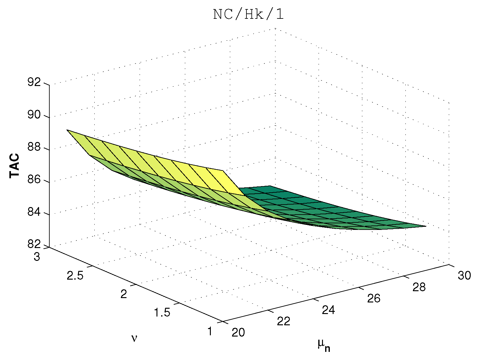
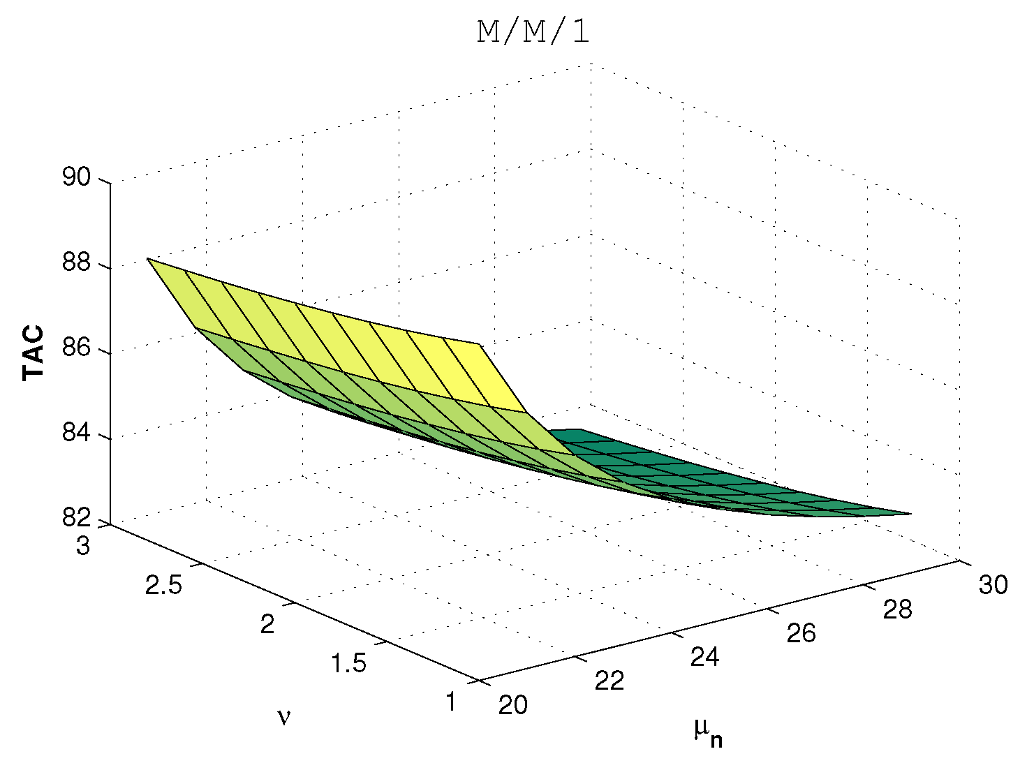
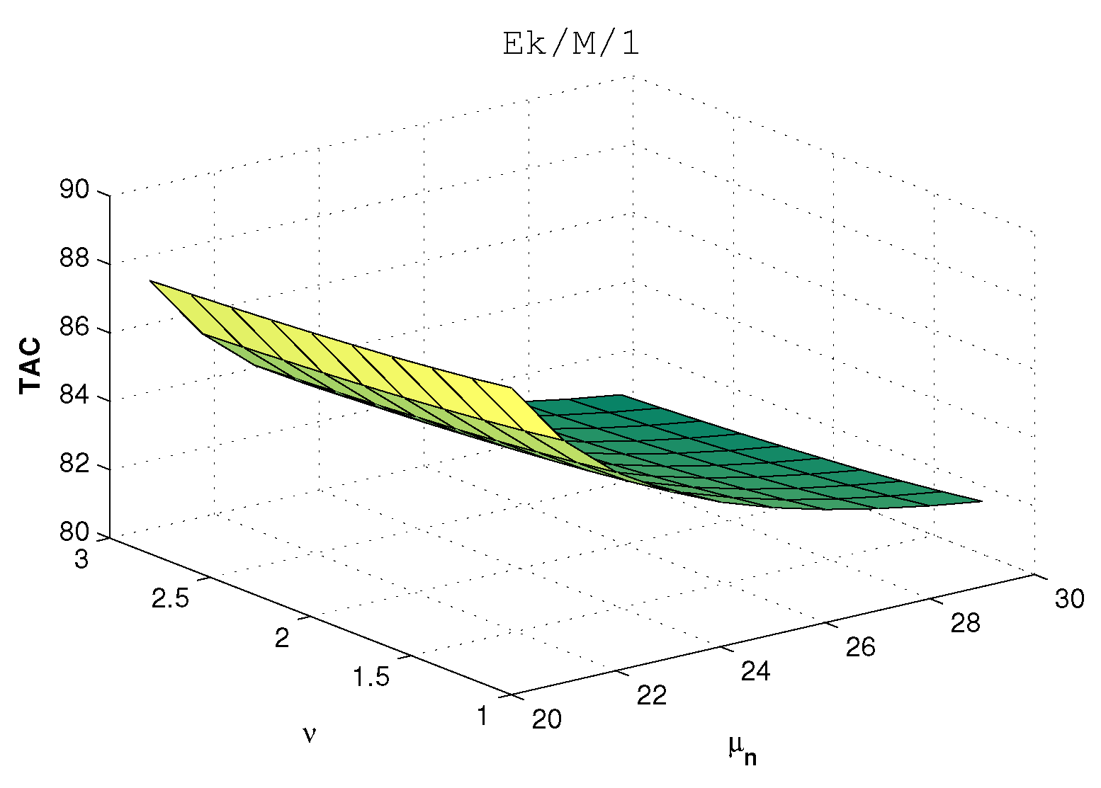
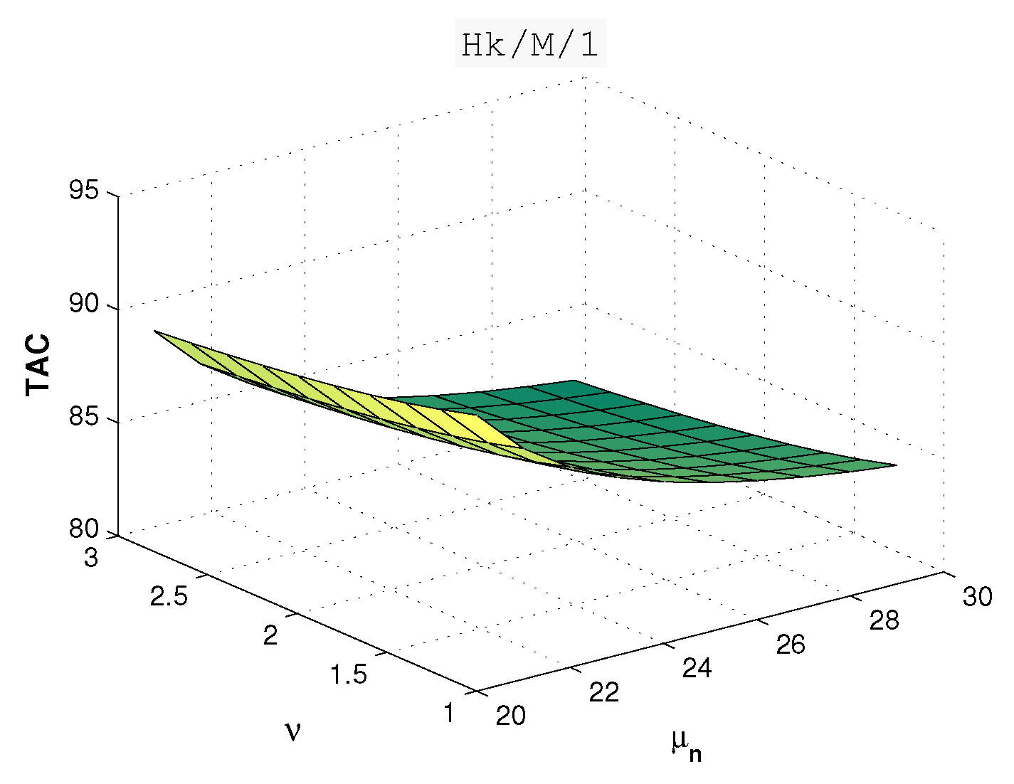
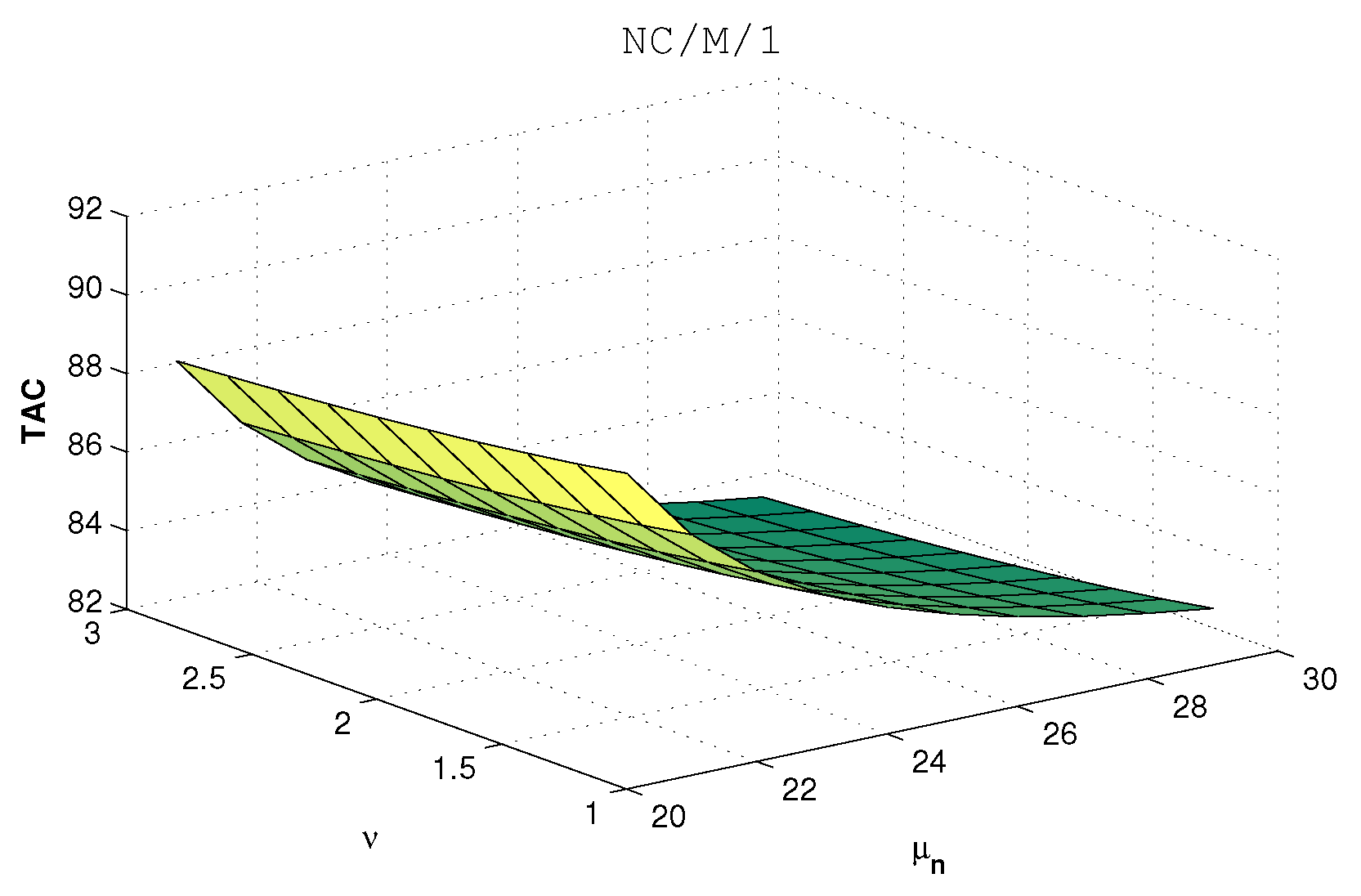
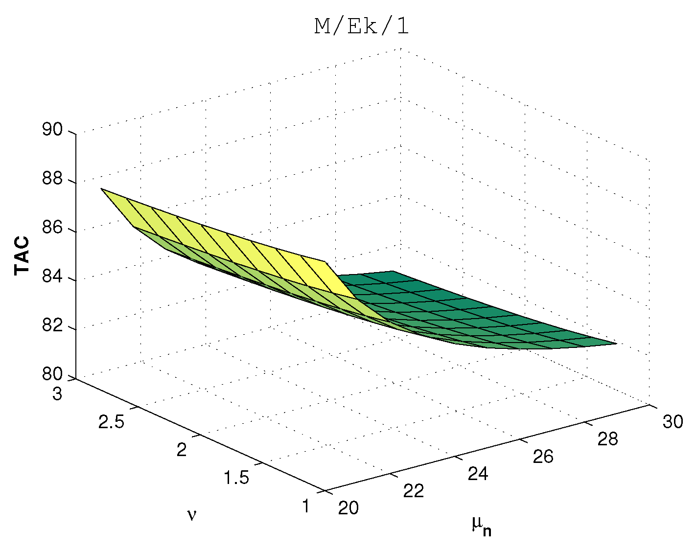
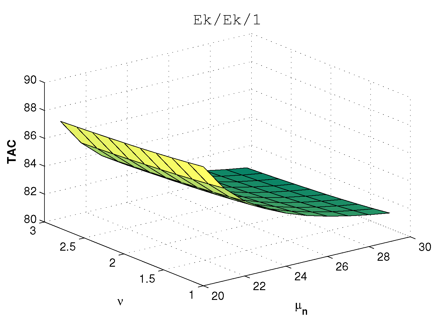
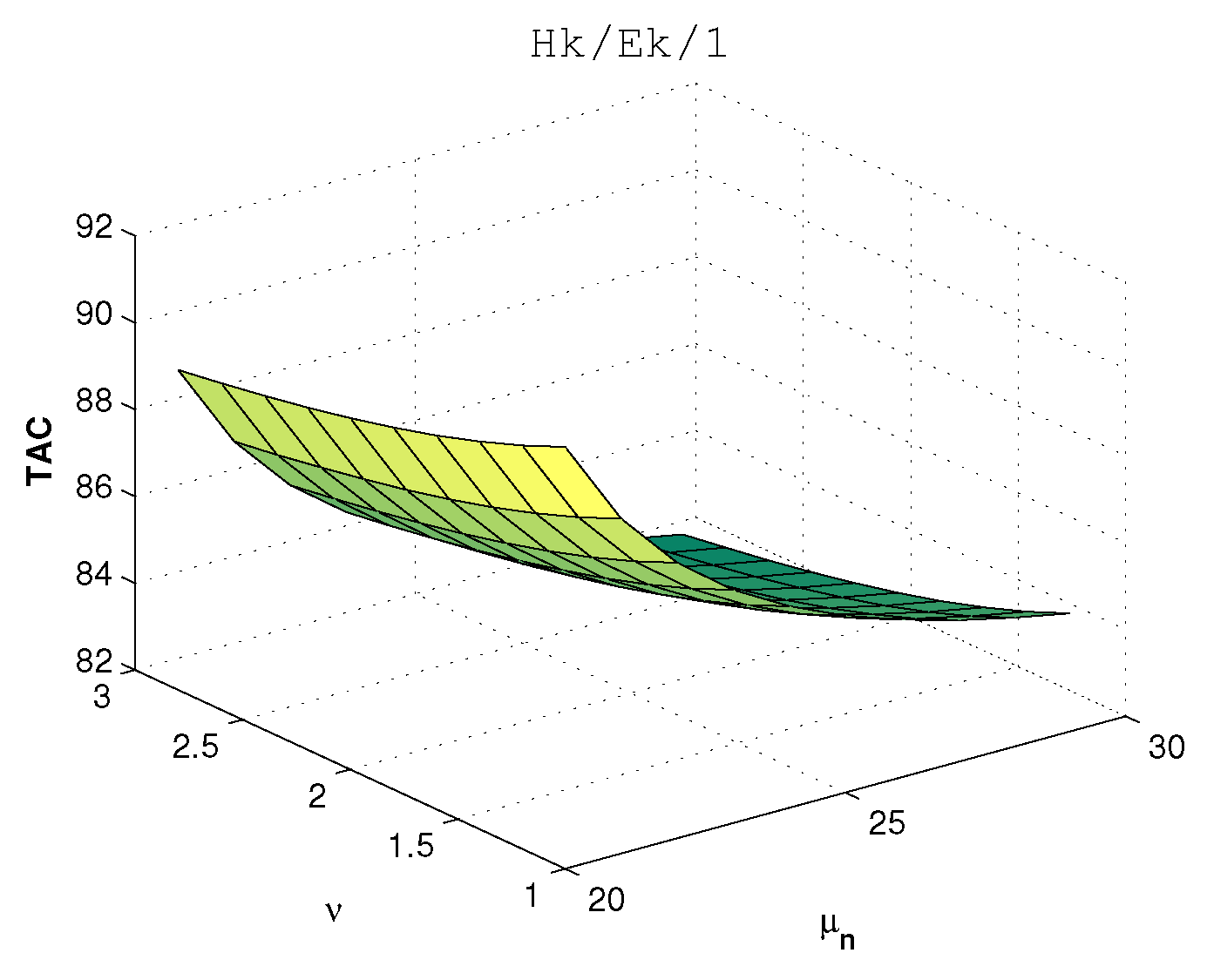
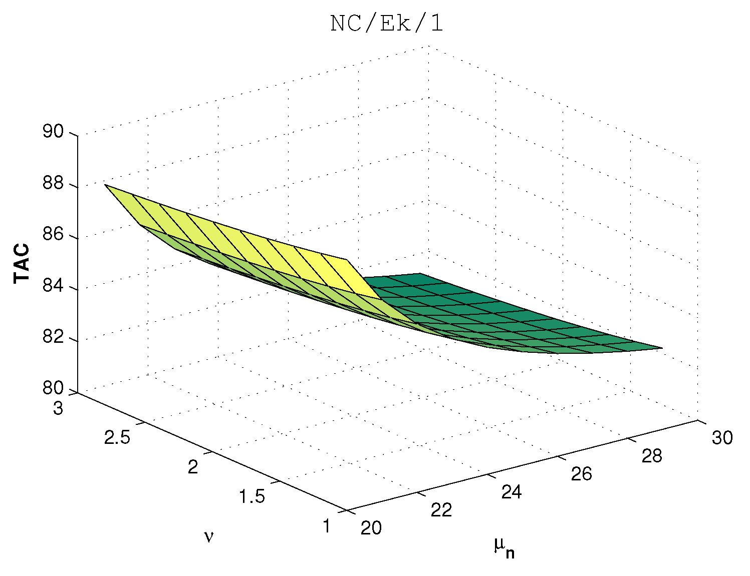
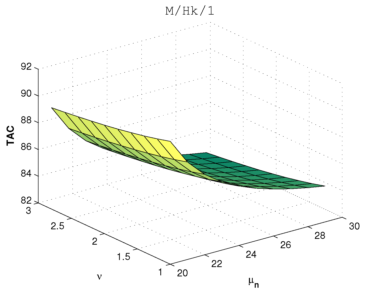
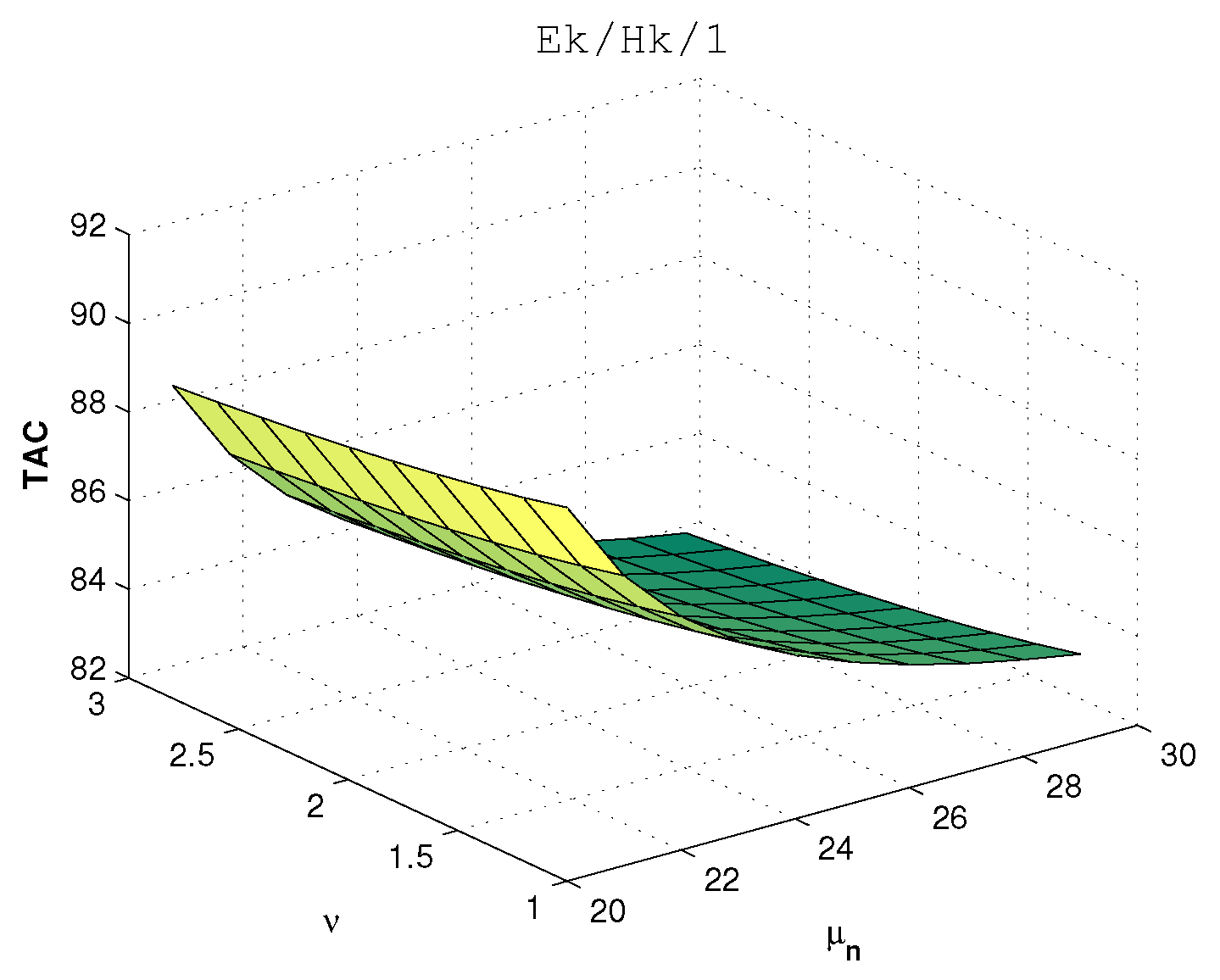
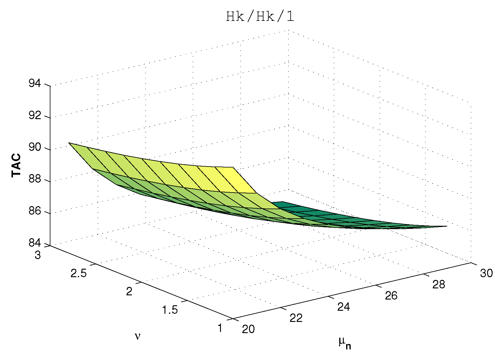
The surface plots reveal a consistent and monotone decrease in TAC as either parameter increases, confirming that faster service completion and more frequent utilization of the vacation mechanism are both effective strategies for reducing the overall operational cost of the system. The reduction in cost with respect to the service rate is theoretically justified, since a higher service rate enables faster processing of customers, thereby reducing queue buildup, waiting time, and holding costs. Similarly, an increase in the vacation rate contributes to cost reduction by allowing the server to enter low-energy states more frequently. This effectively lowers the operating and energy-related expenses, thereby improving the economic efficiency of the system.

The graphical analysis reveals a more pronounced decrease in TAC for the MAP-NC arrival process. This indicates that systems with correlated and bursty arrivals benefit more substantially from improvements in service efficiency and vacation policies. Conversely, the reduction in cost is slower for H-Exp-A. When looking at service-time distributions, Erl-S show a moderate change in total cost due to their structured behavior and lower variability. In contrast, H-Exp-S lead to a sharper change in costs because of their higher variance and fluctuating service durations.

These findings emphasize that both service efficiency and server vacation policies play a vital role in minimizing the total system cost, particularly in systems characterized by highly variable arrival and service processes.

The numerical illustrations presented in Section 7.2, Section 7.3 and Section 7.4 collectively demonstrate the sensitivity of the total average cost (TAC) to variations in arrival intensity, service rates, breakdown rates, repair rates, and vacation parameters across a wide range of distributional assumptions. The results reveal that distributional characteristics of both the arrival and service processes play a decisive role in determining system cost.

These findings offer practically actionable insights for system designers and operations managers seeking to balance service quality, server reliability, and energy efficiency in modern queueing environments such as cloud computing platforms, telecommunication networks, and healthcare service systems. It is anticipated that the analytical framework and cost evaluation methodology developed in this study will serve as a valuable reference for researchers and practitioners engaged in the modeling and optimization of such complex service systems.

7.5. Illustration 5

This subsection presents numerical results for the busy period analysis developed in Section 4, with the objective of providing quantitative insights into the first-passage behavior of the system. The vectors ${\tilde{H}}_1, {\tilde{H}}_2, {\tilde{H}}_1^{(1,0)}, {\tilde{H}}_2^{(1,0)}, {\tilde{H}}_1^{(0,0)}\mathrm{and}{\tilde{H}}_2^{(0,0)}$, defined in Equations (86)–(91), respectively, are evaluated under the parameter settings $\lambda =1,$ ${\mu }_n=20,$ ${\mu }_o=10, {\sigma }_n={\sigma }_o=4, \nu =1, {\upsilon }_n={\upsilon }_o=\upsilon , \zeta =1, \xi =1,\mathrm{and}a=0.4$. The seven entries of each vector correspond to the seven possible server phases at any level $j_1$, namely NS $(j_2=0)$, OS $(j_2=1)$, repair following a breakdown during NS $(j_2=2)$, repair following a breakdown during OS $(j_2=3)$, closedown $(j_2=4)$, vacation $(j_2=5)$, and setup $(j_2=6)$. To examine the influence of the arrival process and server reliability on the busy period metrics, the analysis is carried out across four MAP representations, namely Exp-A, Erl-A, H-Exp-A, and MAP-NC, under two breakdown rates $\upsilon =1$ and $\upsilon =2$, with exponential service and repair distributions. The computed values are reported in

Table 12. Busy Period Analysis under varying arrival distributions and breakdown rates.

Arrival	$\mathit{\upsilon }$	${\mathit{j}}_2$	${\tilde{\mathit{H}}}_1$	${\tilde{\mathit{H}}}_2$	${\tilde{\mathit{H}}}_1^{(1,0)}$	${\tilde{\mathit{H}}}_2^{(1,0)}$	${\tilde{\mathit{H}}}_1^{(0,0)}$	${\tilde{\mathit{H}}}_2^{(0,0)}$
Exp-A	1	0	0.14516	1.29032	0.14516	1.29032	–	–
		1	0.16129	1.32258	0.16129	1.32258	–	–
		2	0.46774	1.93548	0.46774	1.93548	–	–
		3	0.48387	1.96774	0.48387	1.96774	–	–
		4	3.98710	8.77419	3.98710	8.77419	4.07551	7.91398
		5	2.69677	6.19355	2.69677	6.19355	3.25233	6.19355
		6	1.43548	3.87097	1.43548	3.87097	–	–
	2	0	0.18493	1.36986	0.18493	1.36986	–	–
		1	0.20548	1.41096	0.20548	1.41096	–	–
		2	0.52740	2.05479	0.52740	2.05479	–	–
		3	0.54795	2.09589	0.54795	2.09589	–	–
		4	4.25753	9.31507	4.25753	9.31507	4.31943	8.40183
		5	2.88767	6.57534	2.88767	6.57534	3.44323	6.57534
		6	1.55479	4.10959	1.55479	4.10959	–	–
Erl-A	1	0	0.28654	2.54703	0.28654	2.54703	–	–
		1	0.31850	2.60893	0.31850	2.60893	–	–
		2	0.92814	3.80571	0.92814	3.80571	–	–
		3	0.96029	3.86928	0.96029	3.86928	–	–
		4	7.96487	17.46554	7.96487	17.46554	7.95341	15.39825
		5	5.38432	12.30506	5.38432	12.30506	6.17996	11.72309
		6	2.86231	7.66494	2.86231	7.66494	–	–
Erl-A	2	0	0.36455	2.70037	0.36455	2.70037	–	–
		1	0.40524	2.77957	0.40524	2.77957	–	–
		2	1.04484	4.03585	1.04484	4.03585	–	–
		3	1.08579	4.11695	1.08579	4.11695	–	–
		4	8.50251	18.53715	8.50251	18.53715	8.42734	16.34240
		5	5.76291	13.05859	5.76291	13.05859	6.54060	12.44063
		6	3.09790	8.13261	3.09790	8.13261	–	–
H-Exp-A	1	0	0.25736	2.28768	0.25736	2.28768	–	–
		1	0.28595	2.31954	0.28595	2.31954	–	–
		2	0.82867	2.92155	0.82867	2.92155	–	–
		3	0.85722	2.95308	0.85722	2.95308	–	–
		4	7.04662	9.30325	7.04662	9.30325	11.88386	10.20321
		5	4.77996	6.93299	4.77996	6.93299	11.02218	8.98208
		6	2.53587	4.76329	2.53587	4.76329	–	–
	2	0	0.31854	2.35954	0.31854	2.35954	–	–
		1	0.35391	2.39933	0.35391	2.39933	–	–
		2	0.90771	3.02005	0.90771	3.02005	–	–
		3	0.94301	3.05937	0.94301	3.05937	–	–
		4	7.29906	9.62267	7.29906	9.62267	12.16381	10.57643
		5	4.96876	7.17599	4.96876	7.17599	11.26974	9.31883
		6	2.66563	4.93056	2.66563	4.93056	–	–
MAP-NC	1	0	14.42689	128.23904	14.42689	128.23904	–	–
		1	14.53596	128.87523	14.53596	128.87523	–	–
		2	15.76630	133.47825	15.76630	133.47825	–	–
		3	15.81506	133.57834	15.81506	133.57834	–	–
		4	26.11159	152.10301	26.11159	152.10301	26.57008	149.90045
		5	21.28053	135.82694	21.28053	135.82694	23.01763	135.98215
		6	18.66890	139.27910	18.66890	139.27910	–	–
	2	0	18.37884	136.13957	18.37884	136.13957	–	–
		1	18.51757	136.83387	18.51757	136.83387	–	–
		2	19.87847	141.69235	19.87847	141.69235	–	–
		3	19.94056	141.81894	19.94056	141.81894	–	–
		4	30.79755	161.46336	30.79755	161.46336	31.18811	159.12471
		5	25.46488	144.18428	25.46488	144.18428	27.20665	144.34823
		6	22.95971	147.84973	22.95971	147.84973	–	–

.

The entries of ${\tilde{H}}_1$ reveal a clear and intuitive ordering across server phases. The smallest value occurs when the server is actively engaged in NS, confirming that an actively serving system reduces the system size most efficiently. The OS phase yields a marginally higher value, reflecting the additional time required to complete the second stage of service before a departure occurs. Repair phases following breakdowns during NS and OS introduce moderate delays, as the server must complete repair before resuming service. Among all phases, the closedown state incurs the largest mean first-passage time, since the system must sequentially complete closedown, take at least one vacation, undergo setup, and only then serve a customer to achieve a level decrement. The vacation and setup phases yield intermediate values, consistent with the fact that a server in setup is one step closer to resuming service than one still on vacation.

The entries of ${\tilde{H}}_2$ follow a broadly similar ordering to ${\tilde{H}}_1$, with active service phases yielding the smallest values and the closedown phase yielding the highest, reflecting the large number of customers that accumulate during extended server inactivity. An interesting behavior is that although vacation takes more time than setup in ${\tilde{H}}_1$, the setup phase records more service completions than the vacation phase in ${\tilde{H}}_2$. This is because during vacation the server is completely inactive, whereas a server in setup is already preparing to resume service, so customers begin to be processed sooner, leading to more service completions before the system level drops by one.

It is worth noting that in the proposed model, $A_{10}\mathbf{e}=M_2\mathbf{e}$ holds by virtue of $\alpha \mathbf{e}=1$, since $\alpha$ is a probability vector. As established in the literature [38], this condition implies that the mean first-passage behavior from level 1 to level 0 is identical to that from any higher level $j_1\ge 2$, yielding ${\tilde{H}}_1={\tilde{H}}_1^{(1,0)}\mathrm{and}{\tilde{H}}_2={\tilde{H}}_2^{(1,0)}.$

The vectors ${\tilde{H}}_1^{(0,0)}$ and ${\tilde{H}}_2^{(0,0)}$ describe the mean first return time to the empty state and the mean number of service completions during that return, starting from level 0. Two entries are reported corresponding to the closedown and vacation states at level 0. In both cases, starting from the vacation state results in a shorter return time and fewer service completions compared to the closedown state, since the server has already bypassed the closedown stage and is closer to resuming active service.

Across all arrival distributions, increasing the breakdown rate consistently increases all busy period metrics across every server phase, confirming that more frequent breakdowns substantially prolong the busy period. Among the arrival distributions, the MAP-NC process yields the largest busy period values owing to its negative correlation structure, which causes bursty arrivals and greater queue buildup. The Exp-A process produces the smallest values, while Erl-A and H-Exp-A yield intermediate results. These findings highlight that both the correlation structure of the arrival process and server reliability are critical determinants of busy period behavior.

8. Conclusions

This paper presents a comprehensive analytical study of a MAP/PH/1 queueing system with optional supplementary service, server breakdowns with PH distributed repair times, multiple vacations, and closedown and setup periods. By employing PH distributions for both service and repair processes and a MAP, the model effectively captures the variability and correlated bursty behavior of real-world service systems. The system is modeled as a CTMC with a block-structured infinitesimal generator, and matrix-analytic methods are successfully applied to derive the stability condition, stationary probability vector, busy period characteristics, and various system performance measures. A cost analysis framework is also developed to evaluate the economic implications of system operation.

Numerical experiments and special cases confirm the practical relevance of the model and demonstrate its sensitivity to key parameters such as arrival rate, service rates, breakdown rates, and vacation policies. The proposed framework integrates mathematical rigor with analytical tractability, providing valuable insights for both theoretical advancements and real-world system design in areas such as telecommunications, cloud computing, and manufacturing.

Despite its contributions, the model has certain limitations. The closedown, setup, and vacation times are assumed to be exponentially distributed, single correlated arrivals and does not consider customer impatience or retrial behavior. These simplifying assumptions, while necessary for analytical tractability, may limit the model’s applicability in some highly dynamic environments. Future research could extend the current framework in several promising directions. These include incorporating batch arrivals (BMAP), multi-server configurations, priority-based service disciplines, impatient customers, retrial mechanisms and the remaining parameters using PH distributions instead of exponential distributions. Furthermore, we will perform an asymptotic analysis using various performance indicators for the considered queueing system.

Overall, the proposed framework integrates mathematical precision with analytical tractability, offering a structured and practically meaningful approach for the study of complex service systems that is well-suited for both theoretical investigation and real-world system design.

References

Neuts, M.F. A versatile Markovian point process. J. Appl. Probab.1979, 16, 764–779. [Google Scholar] [CrossRef]
Lucantoni, D.M.; Meier-Hellstern, K.S.; Neuts, M.F. A single-server queue with server vacations and a class of non-renewal arrival processes. Adv. Appl. Probab.1990, 22, 676–705. [Google Scholar] [CrossRef]
Lucantoni, D.M. New results on the single server queue with a batch Markovian arrival process. Commun. Stat. Stoch. Model.1991, 7, 1–46. [Google Scholar] [CrossRef]
Neuts, M.F. Models based on the Markovian arrival process. Ieice Trans. Commun.1992, 75, 1255–1265. [Google Scholar]
Chakravarthy, S.R. The batch Markovian arrival process: A review and future work. Adv. Probab. Theory Stoch. Process.2001, 1, 21–49. [Google Scholar]
Artalejo, J.R.; Gómez-Corral, A.; He, Q.M. Markovian arrivals in stochastic modelling: A survey and some new results. Sort-Stat. Oper. Res. Trans.2010, 34, 101–144. [Google Scholar]
Neuts, M.F. Matrix-Geometric Solutions in Stochastic Models: An Algorithmic Approach; Courier Corporation: Chelmsford, MA, USA, 1994. [Google Scholar]
Neuts, M.F. Algorithmic Probability: A Collection of Problems; CRC Press: Boca Raton, FL, USA; Taylor & Francis Group, LLC: Boca Raton, FL, USA, 1995; Volume 3. [Google Scholar]
Neuts, M.F. Structured Stochastic Matrices of M/G/1 Type and Their Applications; CRC Press: Boca Raton, FL, USA; Taylor & Francis Group, LLC: Boca Raton, FL, USA, 2021. [Google Scholar]
Levy, Y.; Yechiali, U. Utilization of idle time in an M/G/1 queueing system. Manag. Sci.1975, 22, 202–211. [Google Scholar] [CrossRef]
Doshi, B.T. Queueing systems with vacation-a survey. Queueing Syst.1986, 1, 29–66. [Google Scholar] [CrossRef]
Takagi, H. Queueing Analysis: A Foundation of Performance Analysis; Volume 1: Vacation and Priority Systems, Part 1; Elsevier Science Publishers B.V.: Amsterdam, The Netherlands, 1991. [Google Scholar]
Tian, N.; Zhang, Z.G. Vacation Queueing Models—Theory and Applications; Springer: New York, NY, USA, 2006. [Google Scholar] [CrossRef]
Ke, J.C.; Wu, C.H.; Zhang, Z.G. Recent developments in vacation queueing models: A short survey. Int. J. Oper. Res.2010, 7, 3–8. [Google Scholar]
Arulmozhi, N.; Haghighi, A.M.; Ayyappan, G.; Archana@ Gurulakshmi, G. Analysis of a crowdsourcing Markovian queue with phase-type and imperfect service, working vacations, breakdown, and repair. Mathematics2025, 13, 3757. [Google Scholar] [CrossRef]
Banik, A.D.; Gupta, U.C.; Pathak, S.S. BMAP/G/1/N queue with vacations and limited service discipline. Appl. Math. Comput.2006, 180, 707–721. [Google Scholar] [CrossRef]
Bharat, D. Generalizations of the stochastic decomposition results for single server queues with vacations. Stoch. Model.1990, 6, 307–333. [Google Scholar] [CrossRef]
Ferrandiz, J.M. The BMAP/GI/1 queue with server set-up times and server vacations. Adv. Appl. Probab.1993, 25, 235–254. [Google Scholar] [CrossRef]
Wu, J.; Liu, Z.; Peng, Y. On the BMAP/G/1 G-queues with second optional service and multiple vacations. Appl. Math. Model.2009, 33, 4314–4325. [Google Scholar] [CrossRef][Green Version]
Aishwarya, N.; Melikov, A.; Ayyappan, G. Analysis of BMAP/PH/c retrial queue with threshold-controlled retrials and synchronous working vacation. Methodol. Comput. Appl. Probab.2026, 28, 10. [Google Scholar] [CrossRef]
Kim, C.; Klimenok, V.I.; Dudin, A.N. Analysis of unreliable BMAP/PH/N type queue with Markovian flow of breakdowns. Appl. Math. Comput.2017, 314, 154–172. [Google Scholar] [CrossRef]
Choudhary, A.; Chakravarthy, S.R.; Sharma, D.C. Impact of the degradation in service rate in MAP/PH/1 queueing system with phase type vacations, breakdowns, and repairs. Ann. Oper. Res.2023, 331, 1207–1248. [Google Scholar] [CrossRef]
Dudin, A.N.; Chakravarthy, S.R.; Dudin, S.A.; Dudina, O.S. Queueing system with server breakdowns and individual customer abandonment. Qual. Technol. Quant. Manag.2024, 21, 441–460. [Google Scholar] [CrossRef]
Madan, K.C. An M/G/1 queueing system with second optional service. Queueing Syst.2000, 34, 37–46. [Google Scholar] [CrossRef]
Medhi, J. A single server Poisson input queue with a second optional channel. Queueing Syst.2002, 42, 239–242. [Google Scholar] [CrossRef]
Wang, J. An M/G/1 queue with second optional service and server breakdowns. Comput. Math. Appl.2004, 47, 1713–1723. [Google Scholar] [CrossRef]
Chakravarthy, S.R. Analysis of MAP/PH1,PH2/1 queue with vacations and optional secondary services. Appl. Math. Model.2013, 37, 8886–8902. [Google Scholar] [CrossRef]
Vijaya Lakshmi, P.; Girija Bhavani, E. Strategic behaviour of customers in a second optional service queue with service interruptions. OPSEARCH2024, 61, 762–784. [Google Scholar] [CrossRef]
Levy, H.; Kleinrock, L. A queue with starter and a queue with vacations: Delay analysis by decomposition. Oper. Res.1986, 34, 426–436. [Google Scholar] [CrossRef]
Bischof, W. Analysis of M/G/1-queues with setup times and vacations under six different service disciplines. Queueing Syst.2001, 39, 265–301. [Google Scholar] [CrossRef]
Gandhi, A.; Doroudi, S.; Harchol-Balter, M.; Scheller-Wolf, A. Exact analysis of the M/M/k/setup class of Markov chains via recursive renewal reward. Queueing Syst.2014, 77, 177–209. [Google Scholar] [CrossRef]
Haghighi, A.M.; Mishev, D.P. A transient M[X]/M(k,K)/1 queue with reneging and setup time for service. Int. J. Math. Oper. Res.2025, 31, 164–181. [Google Scholar] [CrossRef]
Sun, Y.; Ma, Z.; Xu, T. A gated service single vacation M/G/1 queue system with setup and closedown times and different customer arrival rates. Acta Math. Sci.2026, 46, 407–426. [Google Scholar] [CrossRef]
Krishna Kumar, B.; Rukmani, R.; Anantha Lakshmi, S.R. Performance analysis of an M/G/1 queueing system under Bernoulli vacation schedules with server setup and close down periods. Comput. Ind. Eng.2013, 66, 1–9. [Google Scholar] [CrossRef]
Latouche, G.; Ramaswami, V. Introduction to Matrix Analytic Methods in Stochastic Modeling; SIAM Press: Philadelphia, PA, USA, 1999. [Google Scholar] [CrossRef][Green Version]
Artalejo, J.R.; Chakravarthy, S.R.; Lopez-Herrero, M.J. The busy period and the waiting time analysis of a MAP/M/c queue with finite retrial group. Stoch. Anal. Appl.2007, 25, 445–469. [Google Scholar] [CrossRef]
Chakravarthy, S.R. Markovian arrival processes. In Wiley Encyclopedia of Operations Research and Management Science; John Wiley & Sons, Ltd.: Hoboken, NJ, USA, 2011. [Google Scholar] [CrossRef]
Chakravarthy, S.R. Introduction to Matrix-Analytic Methods in Queues 2: Analytical and Simulation Approach—Queues and Simulation; Wiley: Hoboken, NJ, USA, 2022. [Google Scholar] [CrossRef]
Figure 1.
Schematic representation of the model.
Figure 2.
State transition diagram of the proposed queueing model
Figure 3.
TAC vs. and –Exp-A, Exp-S
Figure 4.
TAC vs. and –Erl-A, Exp-S.
Figure 5.
TAC vs. and –H-Exp-A, Exp-S.
Figure 6.
TAC vs. and –MAP-NC, Exp-S.
Figure 7.
TAC vs. and –Exp-A, Erl-S.
Figure 8.
TAC vs. and –Erl-A, Erl-S.
Figure 9.
TAC vs. and –H-Exp-A, Erl-S.
Figure 10.
TAC vs. and –MAP-NC, Erl-S
Figure 11.
TAC vs. and –Exp-A, H-Exp-S.
Figure 12.
TAC vs. and –Erl-A, H-Exp-S.
Figure 13.
TAC vs. and –H-Exp-A, H-Exp-S.
Figure 14.
TAC vs. and –MAP-NC, H-Exp-S.