On the Invariant Subspace Method for Nonlinear Second-Order Evolution Equations

Abstract

We investigate invariant finite-dimensional linear spaces for a class of nonlinear evolution equations with second-order time dependence of the type ${\partial }_{tt}u=-{\partial }_x\left(A(x,u)u\right)+{\partial }_{xx}\left(B(x,u)u\right)+f\left(u\right),$ where the coefficients may depend nonlinearly on the solution. Using direct algebraic verification and invariant subspace reductions, we derive several exact solutions and reduce the governing equations to finite-dimensional systems of ordinary differential equations. Various examples are presented to illustrate the applicability of the method to nonlinear transport, diffusion, and reaction models.

1. Introduction

There are numerous applications of nonlinear partial differential equations (PDEs) involving transport, diffusion, and reaction mechanisms and their interactions in continuum mechanics, physics, and applied science. Nonlinear evolution equations that incorporate both inertial effects and dissipative mechanisms are of significant importance, since they describe the simultaneous presence of wave propagation and diffusion in media. Such phenomena arise in viscoelastic media, nonlinear acoustic waves, and heat conduction with finite propagation speed. For general background on nonlinear wave equations and diffusion processes, we refer to the literature in [1,2,3,4,5].

Nonlinear evolution equations provide an effective modeling tool for viscoelastic media, where stress relaxation and memory effects are present and where wave propagation is influenced by internal damping [6]. In nonlinear acoustics, sound waves with sufficiently large amplitude may undergo distortion, generate harmonics, and lose energy during propagation [7]. The hyperbolic heat conduction equation in the Cattaneo–Vernotte formulation addresses the limitations of Fourier’s law by allowing thermal waves to propagate with finite speed [5]. Nonlinear diffusion–reaction equations also play an important role in biology, particularly in modeling processes such as population dynamics and cancer growth, where spatial diffusion is essential [8]. These models are also widely used in combustion theory to describe flame propagation and thermal instability in reactive systems [9]. In engineering, nonlinear hyperbolic partial differential equations are used to model traffic flow, especially the formation and propagation of shock waves in varying vehicle densities [10]. Such PDEs also play an important role in modeling environmental processes such as groundwater flow and contaminant transport through porous media [11]. Plasma physics and nonlinear optics are two further areas in which similar mathematical tools are used to describe wave–particle interactions and signal propagation in nonlinear media [12,13].

In this work, we study the nonlinear evolution equation

$${\partial }_{tt}u=-{\partial }_x\left(A(x,u)u\right)+{\partial }_{xx}\left(B(x,u)u\right)+f\left(u\right),$$

(1)

where $A(x,u)$ and $B(x,u)$ represent nonlinear transport and diffusion processes, respectively, and $f\left(u\right)$ denotes a nonlinear reaction term. Equation (1) is a quasilinear partial differential equation with both hyperbolic and diffusive features. The second-order time derivative $u_{tt}$ introduces inertial effects and finite propagation speed, while the second-order spatial operator contributes dissipative behavior. As a result, the equation combines features of nonlinear wave equations and diffusion-type models, leading to a rich variety of dynamical behaviors.

Several reductions of Equation (1) connect it with classical models. If $B\equiv 0$ and $f\equiv 0$, then the equation reduces to

$${\partial }_{tt}u=-{\partial }_x\left(A(x,u)u\right),$$

which is a nonlinear wave equation. For suitable choices of the flux function, this includes the classical wave equation as a particular case [2,4]. Nonlinear wave equations of this type are known to exhibit complex phenomena such as finite-time blow-up and global existence, depending on the nonlinear structure; see [14].

If the transport term is neglected, that is, if $A\equiv 0$, then one obtains

$${\partial }_{tt}u={\partial }_{xx}\left(B(x,u)u\right)+f\left(u\right),$$

which retains the second-order time derivative together with a diffusion-type spatial operator. Such equations are closely related to hyperbolic diffusion models and finite-speed heat conduction, including the telegraph equation [5]. In many cases, solutions exhibit a transition from wave-like behavior at short times to diffusion-dominated behavior at large times; see [15].

If the coefficients are independent of u, then Equation (1) takes the semilinear form

$${\partial }_{tt}u=-{\partial }_x\left(A\left(x\right)u\right)+{\partial }_{xx}\left(B\left(x\right)u\right)+f\left(u\right),$$

and, in the case of constant coefficients, it becomes

$${\partial }_{tt}u=-A{\partial }_{x}u+B{\partial }_{xx}u+f\left(u\right).$$

This model combines convection, diffusion, and reaction in a second-order-in-time framework and provides a prototypical example of the interaction between propagation and dissipation. Depending on the relative strength of the different terms, the equation may exhibit either wave-like or diffusion-like behavior.

Equations involving both hyperbolic and diffusive effects have been extensively studied in various contexts, including nonlinear wave equations and reaction–diffusion systems [1,2,16]. Classical reaction–diffusion models such as the Fisher and Kolmogorov–Petrovskii–Piskunov (KPP) equations illustrate the interplay between diffusion and nonlinear reaction mechanisms and play a fundamental role in many applications [17,18]. However, most of these models are parabolic and do not incorporate inertial effects. In contrast, Equation (1) includes both nonlinear transport and second-order time dynamics, leading to a broader class of evolution equations whose analytical structure remains insufficiently understood.

A major challenge in the analysis of nonlinear evolution equations is the derivation of exact solutions. Among the available methods, the invariant subspace approach, originally introduced by Galaktionov [19] and later further developed in [20], has proved to be a powerful and effective tool. The method consists of identifying finite-dimensional linear spaces that remain invariant under the differential operator. This reduces the original partial differential equation to a finite-dimensional system of ordinary differential equations governing the time evolution of the expansion coefficients. Finite-dimensional invariant spaces may be interpreted as reduced dynamical structures capturing dominant modes of the nonlinear evolution equation. In many applications, such reductions provide simplified models that preserve essential nonlinear interactions while allowing explicit analytical treatment. In this sense, the approach is closely related to methods based on symmetry reductions and differential constraints; see [21,22].

Invariant polynomial structures and finite-dimensional invariant spaces have been studied for several classes of nonlinear diffusion equations; see, for example, [23]. These results indicate that nonlinear operators may preserve nontrivial finite-dimensional spaces under suitable structural assumptions. However, explicit invariant finite-dimensional linear subspaces for equations of the form (1), which involve nonlinear transport, nonlinear diffusion, nonlinear reaction, and second-order time evolution, have received comparatively limited attention in the literature. The reaction term $f\left(u\right)$ introduces additional algebraic constraints that significantly affect the invariance properties and therefore require careful analysis.

The aim of this paper is to apply the invariant subspace method to several nonlinear evolution equations of the form (1). We identify nontrivial invariant finite-dimensional linear spaces through direct algebraic verification and use these spaces to reduce the original partial differential equations to finite-dimensional dynamical systems. This approach yields several explicit exact solutions and illustrates how nonlinear transport, diffusion, and reaction terms may interact with invariant structures.

The paper is organized as follows. In Section 2, we briefly recall the invariant subspace method and the corresponding finite-dimensional reduction. In Section 3, we apply the method to several examples and derive explicit solutions, illustrating its effectiveness for the present class of nonlinear evolution equations.

2. Description of the Invariant Subspace Method

In this section, we briefly recall the invariant subspace method, which is a useful tool for constructing particular exact solutions of nonlinear evolution partial differential equations. This method has been applied to various classes of nonlinear diffusion and evolution equations; see, for example, [19,20,23,24].

Consider the general evolution equation

$${\partial }_{tt}u=F\left(u,{\partial }_{x}u,{\partial }_{xx}u,\dots ,{\partial }_{x^k}u\right),k\in {\mathbb{N}}_0:=\mathbb{N}\cup \left\{0\right\},$$

(2)

where $u=u(t,x)$, ${\partial }_x^{i}u={\displaystyle \frac{{\partial }^{i}u}{\partial x^i}}$ denotes the derivative of order i with respect to x, and F is a nonlinear differential operator depending on u and its spatial derivatives.

The basic idea of the method is to look for a finite-dimensional linear space that is preserved by the operator F. Once such a space is identified, the original partial differential equation can be reduced to a finite-dimensional system of ordinary differential equations for the corresponding time-dependent coefficients [19].

Definition 1.

Let $f_1\left(x\right),\dots ,f_n\left(x\right)$ be linearly independent functions, and define

$$W_n=\mathrm{span}\{f_1\left(x\right),\dots ,f_n\left(x\right)\}.$$

The space $W_n$ is called invariant under the operator F if

$$F\left[u\right]\in W_n\mathit{for}\mathit{every}u\in W_n.$$

In the present work, the invariance property is verified directly by substitution into the nonlinear operator associated with each equation. This approach avoids the need for general abstract invariance criteria and focuses instead on explicit algebraic reductions for concrete nonlinear models.

Proposition 1

([20]). Assume that $W_n$ is invariant under the operator F. Then a function of the form

$$u(t,x)={\displaystyle \sum _{i=1}^n}{u}_i\left(t\right)f_i\left(x\right)$$

solves Equation (2) if and only if the coefficient functions $u_i\left(t\right)$ satisfy the system

$$\left\{\begin{array}{c}{\displaystyle \frac{d^2{u}_1}{d{t}^2}}=F_1(u_1,\dots ,u_n),\hfill \\ {\displaystyle \frac{d^2{u}_2}{d{t}^2}}=F_2(u_1,\dots ,u_n),\hfill \\ ⋮\hfill \\ {\displaystyle \frac{d^2{u}_n}{d{t}^2}}=F_n(u_1,\dots ,u_n),\hfill \end{array}\right.$$

(3)

where the functions $F_i$ are determined by the representation

$$F\left({\displaystyle \sum _{i=1}^n}{c}_i{f}_i\left(x\right)\right)={\displaystyle \sum _{i=1}^n}{F}_i(c_1,\dots ,c_n)f_i\left(x\right).$$

This result gives a convenient framework for detecting invariant linear spaces associated with nonlinear differential operators. After such a space has been identified, the original partial differential equation is reduced to a finite-dimensional dynamical system, which in many cases can be analyzed explicitly and may lead to exact closed-form solutions [19,20].

3. Applications

In this section, we present several examples corresponding to different functional forms of the drift and diffusion coefficients to demonstrate the applicability of the method and to clarify the influence of nonlinear transport and diffusion terms on the structure of invariant linear spaces.

Example 1.

Consider the nonlinear partial differential equation

$${\partial }_{tt}u=-{\partial }_x\left(u^2\right)+{\partial }_{xx}u+u^2,t>0,x\in \mathbb{R}.$$

(4)

Let

$$F\left[u\right]:=-{\partial }_x\left(u^2\right)+{\partial }_{xx}u+u^2.$$

We show that the two-dimensional linear space

$$W=\mathrm{span}\{1,e^{x/2}\}$$

is invariant under F. Indeed, for

$$u=y_0+y_1{e}^{x/2},$$

we have

$$F\left[u\right]=y_0^2+\left(y_0+{\displaystyle \frac{1}{4}}\right)y_1{e}^{x/2}\in W.$$

Thus, W is invariant under F.

By Proposition 1, we seek a solution of (4) in the form

$$u(t,x)=y_0\left(t\right)+y_1\left(t\right)e^{x/2}.$$

Substituting into (4), we obtain the reduced system

$$\left\{\begin{array}{c}{y}_0^{″}=y_0^2,\hfill \\ y_1^{″}=\left(y_0+{\displaystyle \frac{1}{4}}\right)y_1.\hfill \end{array}\right.$$

A simple explicit solution of the first equation is

$$y_0\left(t\right)={\displaystyle \frac{6}{{(t-c)}^2}},$$

where c is an arbitrary constant. Hence, the second equation becomes

$$y_1^{″}=\left({\displaystyle \frac{6}{{(t-c)}^2}}+{\displaystyle \frac{1}{4}}\right)y_1.$$

Its general solution is

$$y_1\left(t\right)=C_1{e}^{(t-c)/2}\left(1-{\displaystyle \frac{6}{t-c}}+{\displaystyle \frac{12}{{(t-c)}^2}}\right)+C_2{e}^{-(t-c)/2}\left(1+{\displaystyle \frac{6}{t-c}}+{\displaystyle \frac{12}{{(t-c)}^2}}\right),$$

where $C_1$ and $C_2$ are arbitrary constants.

Therefore, Equation (4) admits the exact solution

$$\begin{array}{cc}\hfill u(t,x)& ={\displaystyle \frac{6}{{(t-c)}^2}}+[C_1{e}^{(t-c)/2}\left(1-{\displaystyle \frac{6}{t-c}}+{\displaystyle \frac{12}{{(t-c)}^2}}\right)\hfill \\ \hfill & +C_2{e}^{-(t-c)/2}\left(1+{\displaystyle \frac{6}{t-c}}+{\displaystyle \frac{12}{{(t-c)}^2}}\right)]e^{x/2}.\hfill \end{array}$$

(5)

In the special case $y_0\equiv 0$, the second equation reduces to

$$y_1^{″}={\displaystyle \frac{1}{4}}{y}_1,$$

whose general solution is

$$y_1\left(t\right)=C_1{e}^{t/2}+C_2{e}^{-t/2}.$$

Thus, another exact solution of (4) is given by

$$u(t,x)=\left(C_1{e}^{t/2}+C_2{e}^{-t/2}\right)e^{x/2}.$$

(6)

To verify the solution, let

$$u(t,x)=y_0\left(t\right)+y_1\left(t\right)e^{x/2}.$$

Then,

$$u_{tt}=y_0^{″}\left(t\right)+y_1^{″}\left(t\right)e^{x/2}.$$

Also, since

$$F\left[u\right]=-{\partial }_x\left(u^2\right)+{\partial }_{xx}u+u^2=y_0^2+\left(y_0+{\displaystyle \frac{1}{4}}\right)y_1{e}^{x/2},$$

the equation $u_{tt}=F\left[u\right]$ is equivalent to

$$y_0^{″}=y_0^2,y_1^{″}=\left(y_0+{\displaystyle \frac{1}{4}}\right)y_1.$$

Therefore, any pair $(y_0,y_1)$ satisfying the reduced system produces an exact solution of Equation (4). Hence, the functions given in (5) and (6) satisfy the original PDE.

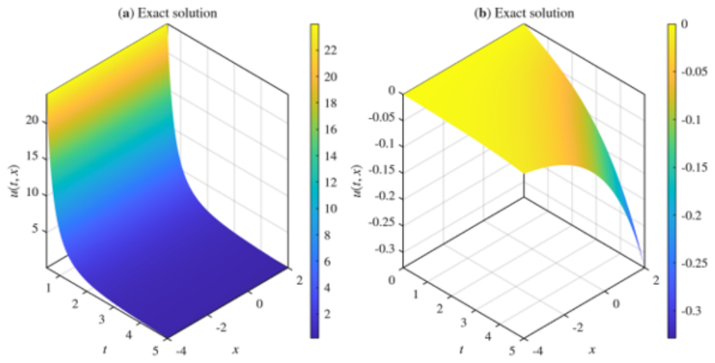
The corresponding solution profiles are illustrated in Figure 1.

Example 2.

Consider the nonlinear partial differential equation

$${\partial }_{tt}u=-{\partial }_x\left({\displaystyle \frac{u^2}{x}}-4xu\right)+{\partial }_{xx}\left(u^2\right).$$

(7)

Let

$$F\left[u\right]:=-{\partial }_x\left({\displaystyle \frac{u^2}{x}}-4xu\right)+{\partial }_{xx}\left(u^2\right).$$

The space

$$\mathcal{W}=\mathrm{span}\left\{x^2\right\}$$

is invariant under F. Indeed, for $u=y{x}^2$, we obtain

$$F\left[y{x}^2\right]=(9y^2+12y)x^2\in \mathcal{W}.$$

Therefore, we seek a solution of (7) in the form

$$u(t,x)=y\left(t\right)x^2.$$

Substituting into (7), we obtain

$$y^{″}=9y^2+12y.$$

In particular, the reduced equation admits the constant solutions

$$y\left(t\right)=0,y\left(t\right)=-{\displaystyle \frac{4}{3}},$$

and the explicit nonconstant solution

$$y\left(t\right)=2{\mathrm{csch}}^2\left(\sqrt{3}t\right).$$

Hence,

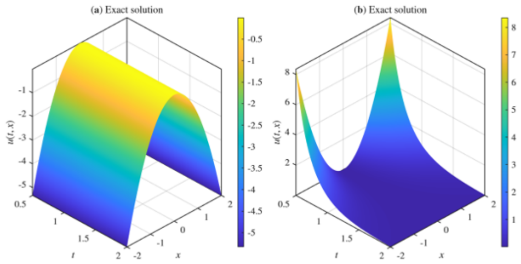
$$u(t,x)=0,u(t,x)=-{\displaystyle \frac{4}{3}}{x}^2,u(t,x)=2x^2{\mathrm{csch}}^2\left(\sqrt{3}t\right)$$

are exact solutions of (7).

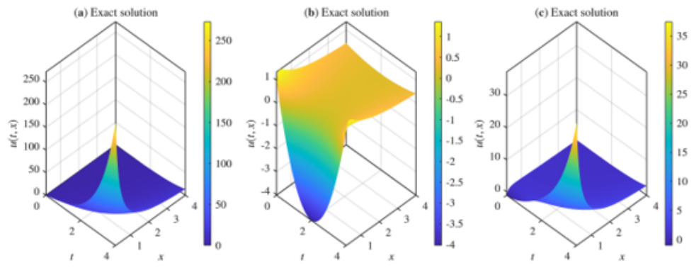
The behavior of the exact solutions is shown in Figure 2.

Example 3.

Consider the nonlinear equation

$${\partial }_{tt}u=-{\partial }_x(u-u^2)+{\partial }_{xx}\left(u^2\right),t>0,x\in \mathbb{R}.$$

(8)

Let

$$F\left[u\right]:=-{\partial }_x(u-u^2)+{\partial }_{xx}\left(u^2\right).$$

Then, the space

$$\mathcal{W}=\mathrm{span}\{1,x\}$$

is invariant under F. Indeed, for $u=y_0+y_{1}x$, a direct computation shows that

$$F[y_0+y_{1}x]=\left(-y_1+2y_0{y}_1+2y_1^2\right)+\left(2y_1^2\right)x\in \mathcal{W}.$$

Therefore, by Proposition 1, we seek a solution of (8) in the form

$$u(t,x)=y_0\left(t\right)+y_1\left(t\right)x.$$

Substituting this form into (8) and identifying the coefficients of 1 and x, we obtain

$$\left\{\begin{array}{c}{\displaystyle y_0^{″}\left(t\right)=-y_1\left(t\right)+2y_0\left(t\right)y_1\left(t\right)+2y_1{\left(t\right)}^2,}\hfill \\ {\displaystyle y_1^{″}\left(t\right)=2y_1{\left(t\right)}^2.}\hfill \end{array}\right.$$

(9)

The second equation has the trivial solution $y_1\equiv 0$, and hence

$$u(t,x)=C_{1}t+C_2.$$

(10)

Moreover, (9) admits no nonzero constant solution for $y_1$. For nonconstant solutions, a first integration yields

$${\left(y_1^{\prime }\left(t\right)\right)}^2={\displaystyle \frac{4}{3}}{y}_1{\left(t\right)}^3+C,C\in \mathbb{R}.$$

Thus the nonconstant solutions are determined implicitly by

$$\int {\displaystyle \frac{d{y}_1}{\sqrt{\frac{4}{3}{y}_1^3+C}}}=\pm t+C_0.$$

In particular, when $C=0$, one obtains the explicit solution

$$y_1\left(t\right)={\displaystyle \frac{3}{{(t-C_0)}^2}}.$$

Substituting this into the first equation in (9), we get

$$y_0^{″}\left(t\right)-{\displaystyle \frac{6}{{(t-C_0)}^2}}{y}_0\left(t\right)=-{\displaystyle \frac{3}{{(t-C_0)}^2}}+{\displaystyle \frac{18}{{(t-C_0)}^4}},$$

whose general solution is

$$y_0\left(t\right)=C_1{(t-C_0)}^3+{\displaystyle \frac{C_2}{{(t-C_0)}^2}}+{\displaystyle \frac{1}{2}}-{\displaystyle \frac{18}{5}}{\displaystyle \frac{\ln |t-C_0|}{{(t-C_0)}^2}}.$$

Consequently,

$$u(t,x)=C_1{(t-C_0)}^3+{\displaystyle \frac{C_2}{{(t-C_0)}^2}}+{\displaystyle \frac{1}{2}}-{\displaystyle \frac{18}{5}}{\displaystyle \frac{\ln |t-C_0|}{{(t-C_0)}^2}}+{\displaystyle \frac{3x}{{(t-C_0)}^2}}$$

(11)

is an exact nontrivial solution of (8), defined on any interval that does not contain $t=C_0$.

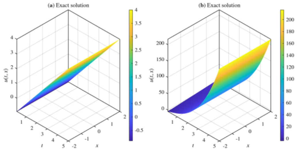
Several explicit exact solutions associated with Equation (8) are displayed in Figure 3.

Example 4.

Consider the nonlinear equation

$${\partial }_{tt}u=-{\partial }_{xx}\left(u^3\right)+u,t>0,x\in \mathbb{R}.$$

(12)

Define the nonlinear operator

$$F\left[u\right]:=-{\partial }_{xx}\left(u^3\right)+u.$$

The two-dimensional linear space

$$\mathcal{W}=\mathrm{span}\{1,x\}$$

is invariant under F. To see this, let

$$u=y_0+y_{1}x.$$

We have

$$u^3={(y_0+y_{1}x)}^3=y_0^3+3y_0^2{y}_{1}x+3y_0{y}_1^2{x}^2+y_1^3{x}^3,$$

and therefore

$${\left(u^3\right)}_{xx}=6y_0{y}_1^2+6y_1^{3}x.$$

It follows that

$$F\left[u\right]=-{\left(u^3\right)}_{xx}+u=\left(y_0-6y_0{y}_1^2\right)+\left(y_1-6y_1^3\right)x\in \mathcal{W}.$$

Hence, $\mathcal{W}$ is invariant under F, and we look for solutions of (12) of the form

$$u(t,x)=y_0\left(t\right)+y_1\left(t\right)x.$$

Upon inserting this expression into (12) and comparing the coefficients of 1 and x, we arrive at

$$\left\{\begin{array}{c}{y}_0^{″}\left(t\right)=y_0\left(t\right)-6y_0\left(t\right)y_1{\left(t\right)}^2,\hfill \\ y_1^{″}\left(t\right)=y_1\left(t\right)-6y_1{\left(t\right)}^3.\hfill \end{array}\right.$$

(13)

A nonconstant solution of the second equation is

$$y_1\left(t\right)=\pm {\displaystyle \frac{1}{\sqrt{3}}}\mathrm{sech}(t-c),c\in \mathbb{R}.$$

Substituting this expression into the first equation gives

$$y_0^{″}\left(t\right)=\left(1-2{\mathrm{sech}}^2(t-c)\right)y_0\left(t\right).$$

A particular solution is

$$y_0\left(t\right)=\mathrm{sech}(t-c).$$

Consequently, (12) admits the explicit exact solution

$$u(t,x)=\mathrm{sech}(t-c)\pm {\displaystyle \frac{1}{\sqrt{3}}}\mathrm{sech}(t-c)x.$$

In addition, the reduced system (13) also yields other simple exact solutions. If $y_1=0$, then $y_0^{″}=y_0$, and we obtain

$$u(t,x)=C_1{e}^t+C_2{e}^{-t}.$$

If $y_1=\pm {\displaystyle \frac{1}{\sqrt{6}}}$, then $y_1^{″}=0$ and the first equation becomes $y_0^{″}=0$, so that

$$u(t,x)=C_1+C_{2}t\pm {\displaystyle \frac{x}{\sqrt{6}}}.$$

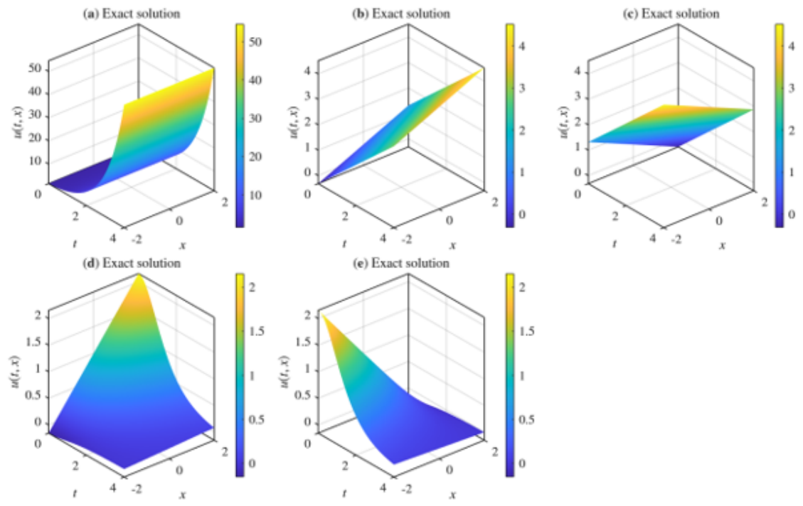
The explicit exact solutions corresponding to Equation (12) are illustrated in Figure 4.

Example 5.

We consider the nonlinear equation

$${\partial }_{tt}u=-{\partial }_x\left(x^2{u}^2\right)+{\partial }_{xx}\left(x^{2}u\right)+u,t>0,x>0.$$

(14)

Define

$$F\left[u\right]=-{\partial }_x\left(x^2{u}^2\right)+{\partial }_{xx}\left(x^{2}u\right)+u.$$

We show that the two-dimensional linear space

$$W=\mathrm{span}\left\{{\displaystyle \frac{1}{x}},{\displaystyle \frac{\ln x}{x}}\right\}$$

is invariant under F.

Indeed, for

$$u(t,x)=x^{-1}\left(y_0\left(t\right)+y_1\left(t\right)\ln x\right),$$

a direct computation gives

$$F\left[u\right]={\displaystyle \frac{y_0+y_1(1-2y_0)}{x}}+{\displaystyle \frac{(y_1-2y_1^2)\ln x}{x}},$$

which belongs to W. Hence, W is invariant, and we seek a solution of (14) in the form

$$u(t,x)=x^{-1}\left(y_0\left(t\right)+y_1\left(t\right)\ln x\right).$$

Substituting this expression into (14) and identifying the coefficients of $x^{-1}$ and $x^{-1}\ln x$, we obtain the reduced system

$$\left\{\begin{array}{c}{y}_0^{″}\left(t\right)=y_0\left(t\right)+y_1\left(t\right)\left(1-2y_0\left(t\right)\right),\hfill \\ y_1^{″}\left(t\right)=y_1\left(t\right)-2y_1{\left(t\right)}^2.\hfill \end{array}\right.$$

(15)

The second equation admits several explicit solutions, which in turn yield exact solutions of the original equation.

Case 1: $y_1\equiv 0$. Then the first equation reduces to

$$y_0^{″}=y_0,$$

and therefore

$$y_0\left(t\right)=C_1{e}^t+C_2{e}^{-t}.$$

Thus,

$$u(t,x)={\displaystyle \frac{C_1{e}^t+C_2{e}^{-t}}{x}}.$$

(16)

Case 2: $y_1\equiv {\displaystyle \frac{1}{2}}$. Then

$$y_0^{″}={\displaystyle \frac{1}{2}},$$

so that

$$y_0\left(t\right)={\displaystyle \frac{1}{4}}{t}^2+C_{1}t+C_2.$$

Hence,

$$u(t,x)={\displaystyle \frac{\frac{1}{4}{t}^2+C_{1}t+C_2+\frac{1}{2}\ln x}{x}}.$$

(17)

Case 3: A nonconstant solution. A nonconstant solution of the second equation is

$$y_1\left(t\right)={\displaystyle \frac{3}{4}}{\mathrm{sech}}^2\left({\displaystyle \frac{t-c}{2}}\right),c\in \mathbb{R}.$$

A direct computation verifies that this function satisfies

$$y_1^{″}=y_1-2y_1^2.$$

For this choice, the first equation becomes

$$y_0^{″}+\left(2y_1\left(t\right)-1\right)y_0=y_1\left(t\right).$$

A corresponding particular solution is

$$y_0\left(t\right)={\displaystyle \frac{1}{2}}+{\displaystyle \frac{1}{2}}{\cosh }^2\left({\displaystyle \frac{t-c}{2}}\right).$$

Therefore, (14) admits the exact solution

$$u(t,x)={\displaystyle \frac{1}{x}}\left({\displaystyle \frac{1}{2}}+{\displaystyle \frac{1}{2}}{\cosh }^2\left({\displaystyle \frac{t-c}{2}}\right)+{\displaystyle \frac{3}{4}}{\mathrm{sech}}^2\left({\displaystyle \frac{t-c}{2}}\right)\ln x\right).$$

(18)

Therefore, the invariant subspace approach leads to several explicit exact solutions of (14), ranging from elementary solutions to nonconstant ones.

Several explicit solutions associated with Equation (14) are displayed in Figure 5.

Example 6.

Consider the nonlinear wave-type equation

$${\partial }_{tt}u=-{\partial }_{x}u+{\partial }_{xx}\left(u^2\right)-u,t>0,x\in \mathbb{R}.$$

(19)

Define the nonlinear operator

$$F\left[u\right]=-{\partial }_{x}u+{\partial }_{xx}\left(u^2\right)-u.$$

We verify that the two-dimensional linear space

$$W=\mathrm{span}\{1,x\}$$

is invariant under F. Indeed, for

$$u(t,x)=y_0\left(t\right)+y_1\left(t\right)x,$$

a direct computation gives

$$F\left[u\right]=(2y_1^2-y_1-y_0)-y_{1}x\in W.$$

Hence, W is invariant under F. Therefore, seeking a solution in the form

$$u(t,x)=y_0\left(t\right)+y_1\left(t\right)x,$$

the equation

$${\partial }_{tt}u=F\left[u\right]$$

reduces to the system

$$\left\{\begin{array}{c}{y}_0^{″}=2y_1^2-y_1-y_0,\hfill \\ y_1^{″}=-y_1.\hfill \end{array}\right.$$

The second equation has the general solution

$$y_1\left(t\right)=A\cos t+B\sin t.$$

Substituting this expression into the first equation yields

$$y_0^{″}+y_0=2y_1^2-y_1.$$

Solving this equation, we obtain the explicit family of exact solutions

$$\begin{array}{cc}\hfill u(t,x)=& C_1\cos t+C_2\sin t+(A^2+B^2)-{\displaystyle \frac{A^2-B^2}{3}}\cos 2t-{\displaystyle \frac{2AB}{3}}\sin 2t\hfill \\ \hfill & -{\displaystyle \frac{A}{2}}t\sin t+{\displaystyle \frac{B}{2}}t\cos t+\left(A\cos t+B\sin t\right)x,\hfill \end{array}$$

(20)

where $A,B,C_1,C_2\in \mathbb{R}$.

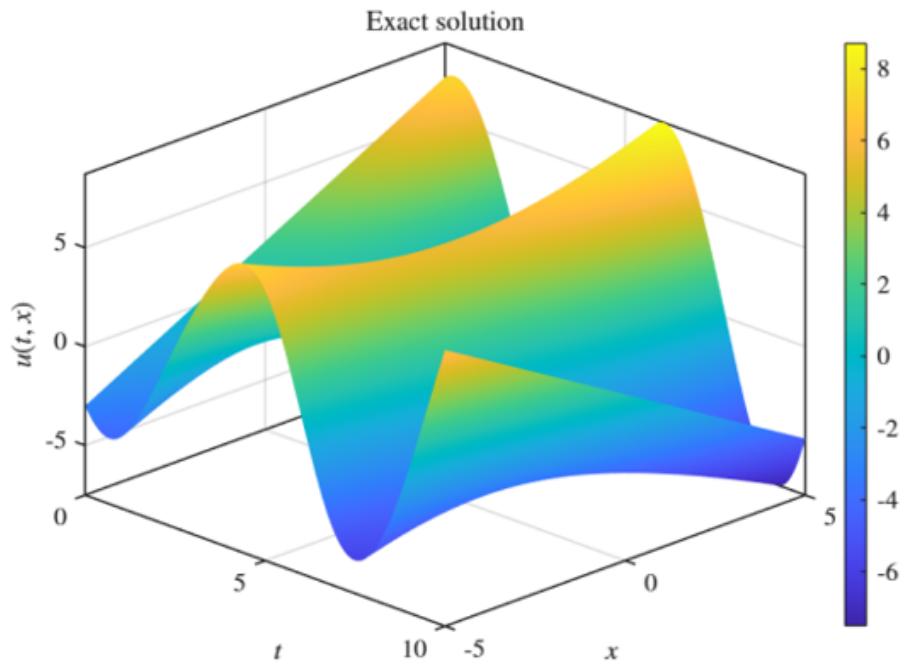
The solution family corresponding to Equation (19) is illustrated in Figure 6.

4. Conclusions

In this paper, we studied invariant finite-dimensional linear subspaces for a class of nonlinear evolution equations with second-order time dependence of the form

$${\partial }_{tt}u=-{\partial }_x\left(A(x,u)u\right)+{\partial }_{xx}\left(B(x,u)u\right)+f\left(u\right).$$

We investigated several invariant finite-dimensional linear spaces associated with nonlinear evolution equations possessing second-order time dependence. For each example, the original partial differential equation is reduced to a finite-dimensional system of ordinary differential equations governing the time-dependent coefficients of the solution.

The invariant subspace reductions considered in this work provide a constructive approach for obtaining explicit exact solutions of several nonlinear evolution equations. The examples demonstrate that the method applies to several nonlinear transport, diffusion, and reaction models and can generate nontrivial invariant structures together with explicit exact solutions. All explicit solutions obtained in the examples can be verified directly by substitution into the corresponding nonlinear evolution equations. These results show that invariant subspaces remain an effective tool for the analysis of nonlinear evolution equations and for the explicit construction of exact solutions.

Future work may address higher-dimensional settings, more general nonlinearities, and broader classes of invariant spaces, as well as possible applications to physically motivated models arising in mechanics, diffusion theory, and nonlinear wave propagation. Future developments may also include observer-based formulations for partially measurable systems and more general classes of delayed nonlinear evolution equations.

References

1. Evans, L.C. Partial Differential Equations, 2nd ed.; American Mathematical Society: Providence, RI, USA, 2010. [Google Scholar]
2. Smoller, J. Shock Waves and Reaction–Diffusion Equations; Springer: New York, NY, USA, 1983. [Google Scholar]
3. Logan, J.D. An Introduction to Nonlinear Partial Differential Equations; Wiley: New York, NY, USA, 1994. [Google Scholar]
4. Strauss, W.A. Nonlinear Wave Equations; Regional Conference Series in Mathematics; American Mathematical Society: Providence, RI, USA, 1989; Volume 73. [Google Scholar]
5. Joseph, D.D.; Preziosi, L. Heat waves. Rev. Mod. Phys. 1989, 61, 41–73. [Google Scholar] [CrossRef] [Scilit]
6. Christensen, R.M. Theory of Viscosity; Academic Press: New York, NY, USA, 1982. [Google Scholar]
7. Hamilton, M.F.; Blackstock, D.T. Nonlinear Acoustics; Academic Press: San Diego, CA, USA, 1998. [Google Scholar]
8. Murray, J.D. Mathematical Biology I: An Introduction; Springer: New York, NY, USA, 2002. [Google Scholar]
9. Zeldovich, Y.B.; Barenblatt, G.I. Theory of flame propagation. Combust. Flame 1959, 3, 61. [Google Scholar]
10. Lighthill, M.J.; Whitham, G.B. On kinematic waves. II. A theory of traffic flow. Proc. R. Soc. Lond. A 1955, 229, 317. [Google Scholar] [CrossRef] [Scilit]
11. Bear, J. Dynamics of Fluids in Porous Media; Elsevier: New York, NY, USA, 1972. [Google Scholar]
12. Chen, F.F. Introduction to Plasma Physics and Controlled Fusion; Springer: Cham, Switzerland, 2016. [Google Scholar]
13. Agrawal, G.P. Nonlinear Fiber Optics; Academic Press: Waltham, MA, USA, 2013. [Google Scholar]
14. Glassey, R.T. Finite-time blow-up for solutions of nonlinear wave equations. Math. Z. 1981, 177, 323–340. [Google Scholar] [CrossRef] [Scilit]
15. Nishihara, K. Asymptotic behavior of solutions to the semilinear wave equation with time-dependent damping. Tokyo J. Math. 2011, 34, 327–343. [Google Scholar] [CrossRef] [Scilit]
16. Barles, G.; Evans, L.C.; Souganidis, P.E. Wavefront propagation for reaction–diffusion systems of PDEs. Duke Math. J. 1990, 61, 835–858. [Google Scholar] [CrossRef] [Scilit]
17. Fisher, R.A. The wave of advance of advantageous genes. Ann. Eugen. 1937, 7, 355–369. [Google Scholar] [CrossRef] [Scilit]
18. Kolmogorov, A.; Petrovskii, I.; Piskunov, N. Study of the diffusion equation with growth of the quantity of matter, and its application to a biological problem. Byul. Mosk. Gos. Univ. Ser. A Mat. Mekh. 1937, 1, 1–26. [Google Scholar]
19. Galaktionov, V.A. Invariant subspaces and new explicit solutions to evolution equations with quadratic nonlinearities. Proc. R. Soc. Edinb. Sect. A 1995, 125, 225–246. [Google Scholar] [CrossRef] [Scilit]
20. Galaktionov, V.A.; Svirshchevskii, S.R. Exact Solutions and Invariant Subspaces of Nonlinear Partial Differential Equations; Chapman & Hall/CRC: Boca Raton, FL, USA, 2007. [Google Scholar]
21. Olver, P.J. Applications of Lie Groups to Differential Equations, 2nd ed.; Springer: New York, NY, USA, 1993. [Google Scholar]
22. Clarkson, P.A.; Kruskal, M.D. New similarity reductions of the Boussinesq equation. J. Math. Phys. 1989, 30, 2201–2213. [Google Scholar] [CrossRef] [Scilit]
23. King, J.R. Exact polynomial solutions to some nonlinear diffusion equations. J. Phys. A Math. Gen. 1993, 26, 5079–5090. [Google Scholar]
24. Ma, W.X. A refined invariant subspace method and applications to evolution equations. Sci. China Math. 2012, 55, 1769–1778. [Google Scholar] [CrossRef] [Scilit]
Figure 1. (a) Exact solution (5) corresponding to c = 0 , C 1 = 0.01 , and C 2 = 0.01 ; (b) Exact solution (6) corresponding to C 1 = 0.01 and C 2 = 0.01 .
Mathematics 14 02155 g001
Figure 2. Exact Solutions of (7).
Mathematics 14 02155 g002
Figure 3. (a) Exact Solution (10), (b) Exact Solution (11), C 0 = 1 ; C 1 = 1 , C 2 = 1 .
Mathematics 14 02155 g003
Figure 4. Explicit exact solutions of Equation (12): (a) u ( t , x ) = e t + 0.5 e t ; (b) u ( t , x ) = 0.5 + 0.8 t + x 6 ; (c) u ( t , x ) = 0.5 + 0.8 t x 6 ; (d) u ( t , x ) = sech ( t ) + 1 3 sech ( t ) x ; (e) u ( t , x ) = sech ( t ) 1 3 sech ( t ) x .
Mathematics 14 02155 g004
Figure 5. Explicit exact solutions of Equation (14): (a) Exact solution (16); (b) Exact solution (17); (c) Exact solution (18).
Mathematics 14 02155 g005
Figure 6. Explicit Exact Solutions of (19).
Mathematics 14 02155 g006
Disclaimer/Publisher’s Note: The statements, opinions and data contained in all publications are solely those of the individual author(s) and contributor(s) and not of MDPI and/or the editor(s). MDPI and/or the editor(s) disclaim responsibility for any injury to people or property resulting from any ideas, methods, instructions or products referred to in the content.