HMT-Net: A Hybrid Mamba–Transformer Network for Motor Imagery EEG Decoding

Abstract

Electroencephalography (EEG) is widely used in brain-computer interfaces (BCIs) for decoding motor imagery (MI) signals. However, existing methods remain limited in extracting multi-scale local spatiotemporal features and effectively integrating them with global feature information, leaving room for further improvement in classification accuracy. To address this issue, we propose HMT-Net, a hybrid architecture that integrates multi-scale convolution, the Mamba state-space model, and a self-attention mechanism. The model consists of a shallow feature embedding (SFE) module for spatiotemporal feature extraction, a multi-scale local feature extractor (MSLFE), and a Mamba–transformer global feature encoder (MTGFE). Specifically, the MSLFE employs dual-branch convolutions and channel attention to achieve adaptive multi-scale perception, while the MTGFE combines Mamba’s linear sequence modeling capability with multi-head attention to efficiently capture global dependencies. Unlike conventional Mamba or transformer EEG models, HMT-Net couples linear state-space modeling with global pairwise attention, avoiding the representational limits inherent in each individual architecture. Experiments on the BCI-IV-2a, BCI-IV-2b, and HGD datasets show that HMT-Net achieves subject-dependent accuracies of 84.07%, 89.60%, and 96.02%, respectively, outperforming EEGNet, FBCNet, EEGConformer, and ATCNet by 11.65%, 5.02%, 5.13%, and 6.60%, respectively, on BCI-IV-2a. Furthermore, HMT-Net achieves the best accuracy in subject-independent experiments, demonstrating strong generalization capability. Ablation studies and visualizations further validate the effectiveness and interpretability of the proposed model.

1. Introduction

In recent years, brain-computer interface (BCI) technology has become an important focus of research at the intersection of neuroscience and artificial intelligence, owing to its great potential for establishing direct communication pathways between the brain and external environments [1,2]. Among various acquisition modalities, scalp electroencephalography (EEG) has become a preferred technique for capturing central nervous system activity due to its non-invasiveness, high temporal resolution, and ease of deployment [3,4]. In particular, the motor imagery (MI) paradigm, which decodes motor intentions by evoking sensorimotor rhythms (SMRs) in the cerebral cortex, has shown broad application prospects in clinical rehabilitation and neuro-assistance [5,6,7]. However, MI-EEG signals are characterized by an extremely low signal-to-noise ratio (SNR) and high non-stationarity [8,9]. Therefore, how to effectively extract discriminative features that preserve both local details and global dependencies from complex non-stationary MI-EEG signals remains a key issue for improving motor imagery decoding performance.

With advancements in deep learning, researchers have proposed various methods to address these challenges [10]. Convolutional neural networks (CNNs), such as EEGNet [11] and ShallowConvNet [12], can effectively capture local short-range features by eliminating the need for tedious traditional feature engineering. However, restricted by the inherent local receptive fields of convolutional kernels, CNNs struggle to effectively capture global dynamic features spanning long temporal scales [13]. To overcome this bottleneck, transformer architectures based on self-attention mechanisms, such as EEGConformer [14] and ATCNet [15], have been introduced to MI-EEG decoding, significantly enhancing the collaborative representation of local details and global correlations [16,17]. However, although transformers can effectively model global dependencies, their feature extraction capabilities mainly rely on self-attention mechanisms and provide relatively weak inductive bias for local spatiotemporal structures, which may limit their ability to capture detailed and multi-scale local physiological patterns in MI-EEG signals. Recently, the Mamba architecture [18], built upon structured state-space models (SSMs) [19], has achieved efficient global modeling with linear complexity, effectively reducing computational burden. However, transformers demand quadratic computational overhead, while pure Mamba models compress historical states sequentially, occasionally losing fine-grained, non-local temporal correlations. Although these methods improve MI-EEG representation learning from different perspectives, structures based on a single or dominant modeling mechanism still struggle to fully accommodate the coexistence of local transient variations and global dynamic representations in MI-EEG signals.

Specifically, effective MI-EEG features are mainly reflected in two aspects: local multi-scale features and global long-range dependencies. On the one hand, SMR induced by motor imagery exhibits significant multi-scale transient variations along spatiotemporal dimensions [20,21], while volume conduction effects and redundant channel noise during electrode acquisition may weaken the expression of critical physiological information [22]. Therefore, the model needs multi-scale local perception capability in order to extract discriminative local spatiotemporal patterns from different receptive fields and emphasize key channel responses. On the other hand, motor imagery involves sustained and coordinated neural dynamic evolution across multiple brain regions, and the core discriminative information is often embedded in long-range nonlinear dependencies [23]. This requires the model to effectively capture temporal contextual information from a global perspective. Although existing methods have made progress in local feature extraction or global long-range modeling, they remain limited in coordinating multi-scale local perception with global long-range modeling, thereby constraining the discriminative feature representation capability of MI-EEG signals and the further improvement of decoding accuracy.

Thus, the remaining challenge is less about replacing one sequence model with another than about how local and global information are computed and coupled. After shallow spatiotemporal embedding, an EEG trial is first represented as $F_{\mathrm{SFE}}\in {\mathbb{R}}^{p\times k}$, where p denotes the number of temporal positions and k denotes the number of feature channels. With learnable positional encoding, the position-enhanced token sequence is obtained as $F_{\mathrm{PE}}={\mathrm{PE}}_{\mathrm{learn}}\left(F_{\mathrm{SFE}}\right)$. Class-related patterns in this sequence are not confined to a single temporal scale; short transient SMR variations and local patterns with broader receptive fields may coexist along the trial. Therefore, $F_{\mathrm{PE}}$ should be mapped by two depthwise temporal branches into the scale-specific responses $F_{r_1}$ and $F_{r_2}$ before global dependency modeling. Since different channels and scales contribute unequally under low-SNR and non-stationary EEG conditions, these responses also require adaptive channel recalibration before fusion. After this multi-scale local refinement, the resulting sequence, $F_{\mathrm{MSLFE}}$, still requires global modeling because motor imagery involves continuous temporal evolution and interactions among different temporal segments. Therefore, the key issues are how to construct adaptive multi-scale local representations and how to integrate them with efficient global dependency modeling. However, existing transformer-based EEG classifiers primarily rely on self-attention, which lacks sufficient local inductive bias to capture transient, multi-scale SMR fluctuations. Conversely, emerging Mamba-based EEG models, while efficient at continuous sequence scanning, struggle to capture explicit, non-local segment-to-segment pairwise temporal alignments across distant brain activity states. Consequently, single-mechanism structures remain fundamentally limited in reconciling both local multi-scale transient dynamics and complex global temporal associations.

To address these issues, this paper proposes a Hybrid Mamba–Transformer Network (HMT-Net). The proposed model integrates multi-scale convolution, state-space models, and self-attention mechanisms to comprehensively capture both fine-grained local features and the long-range global dependencies of MI-EEG signals. The primary novelty of HMT-Net, distinguishing it from conventional Mamba- or transformer-dominant architectures, lies in a dual-level coupling strategy. First, at the local level, instead of using standard convolutional embeddings, we propose the MSLFE. The MSLFE utilizes parallel, depthwise temporal convolutions to capture multi-scale localized transient variations followed by channel attention to adaptively recalibrate feature responses under noisy EEG conditions. Second, at the global level, unlike models that deploy Mamba and transformer layers in isolation, we design the MTGFE. By sequentially chaining bidirectional state-space tracking with multi-head self-attention, the MTGFE allows Mamba’s continuous scanning to construct temporal contexts, which guide the self-attention mechanism in establishing precise global pairwise alignments. HMT-Net consists of three core components: first, a preliminary mapping layer completes the foundational topological fusion of electrode space and time series; second, a multi-scale local feature extractor (MSLFE) is introduced to extract transient physiological features via multi-branch dynamic receptive fields and channel attention; finally, a Mamba–transformer global feature encoder (MTGFE) is constructed to synergize linear continuous state evolution with discrete global attention.

The main contributions of this paper are summarized as follows:

• Proposed the HMT-Net Hybrid Feature Extraction Framework: This framework establishes a hierarchical spatio-temporal route. By organically fusing local details from convolutional perception with global long-range associations from Mamba and transformers, it achieves precise modeling of cross-channel spatial features and non-stationary temporal evolution, significantly improving the extraction accuracy of discriminative features.
• Designed a Multi-Scale Local Feature Extractor (MSLFE) with Dynamic Receptive Fields: This module utilizes dual-branch convolutions and a channel attention mechanism to dynamically weight multi-scale features, significantly enhancing the model’s ability to extract local physiological features in low-SNR environments.
• Innovatively Proposed a hybrid Mamba–transformer global feature encoder (MTGFE): We deeply integrate Multi-Head Attention (MHA) and the Mamba state-space model within the transformer architecture. This fused structure enhances the model’s ability to capture global contextual information and long-range spatial dependencies, leading to a significant boost in decoding accuracy.
• Validated Effectiveness through Extensive Evaluations: Through extensive significance tests, inter-block ablation studies, ablation studies on transformer and Mamba, parameter analysis, and visualization experiments, we systematically evaluate the contributions of the proposed MSLFE module and the collaborative Mamba–attention structure in the MTGFE module. The results show that the MSLFE effectively enhances local spatio-temporal feature extraction, whereas the MTGFE improves global dependency modeling. These analyses further demonstrate that the collaboration between local feature extraction and global context modeling is essential for accurate and robust MI-EEG decoding.

The remainder of this paper is organized as follows. Section 2 reviews related work. Section 3 introduces the proposed method. Section 4 presents the experimental setup. Section 5 reports the experimental results and analysis. Section 6 provides further discussion. Finally, Section 7 concludes this paper.

2. Related Work

2.1. Local Feature Extraction Based on Convolutional Neural Networks

Over the past five years, deep learning methods have achieved remarkable progress in the field of motor imagery electroencephalography (MI-EEG) classification, owing to their powerful capabilities in automatic feature learning and multi-layer abstract representation. Specifically, convolutional neural networks (CNNs) have established themselves as a cornerstone of MI-EEG decoding due to their inherent ability to extract local features. For instance, Lawhern et al. proposed the EEGNet model [11], which achieves a superior balance between parameter efficiency and decoding performance by introducing depthwise separable convolutions. Schirrmeister et al. designed ShallowConvNet and DeepConvNet [12], establishing a benchmark framework for end-to-end processing of raw EEG signals by simulating the feature mapping logic of filter banks. To further capture multi-frequency information, Mane et al. developed the FBCNet model [24], which leverages a multi-branch convolutional architecture to strengthen the representation of multi-band spatial information. Addressing the low signal-to-noise ratio characteristic of MI-EEG, Li et al. proposed the TS-SEFFNet model [25], which integrates a temporal-spectral squeeze-and-excitation feature fusion mechanism to significantly enhance the stability of key physiological features through dynamic recalibration. Despite the excellent performance of existing CNN-based models in capturing local transient patterns, they suffer from a significant limitation: restricted by the fixed receptive field of convolutional kernels, these methods often struggle to effectively capture the complex temporal evolution of brain activity during long-duration cognitive tasks.

2.2. Global Dependency Modeling Based on Transformers and State-Space Models

To compensate for the limitations of CNNs in extracting long-range temporal features, researchers have introduced global sequence modeling architectures into MI-EEG decoding. From a feature extraction perspective, transformer-based models employ self-attention mechanisms to establish interactions among temporal tokens, thereby aggregating contextual information and enhancing the representation of dependencies among distributed EEG segments. For example, Altaheri et al. proposed ATCNet [15], which combines temporal convolutional networks (TCNs) with sliding-window multi-head attention to extract discriminative temporal features. Song et al. designed EEG-Conformer [14], which integrates convolutional local feature extraction with transformer-based contextual feature refinement to improve MI-EEG representation. Zhang et al. further proposed a local and global convolutional transformer architecture [16], in which dual-scale transformer encoders are used to extract local temporal patterns and long-range global features. In addition, Zhao et al. introduced TMSA-Net [17], embedding multi-scale convolution into the self-attention module to enhance feature extraction from different receptive fields.

Although transformer-based methods improve the extraction of global contextual features, their representation learning still largely depends on attention-driven token interactions. Such a mechanism is effective for modeling relationships among temporal segments, but it provides relatively limited intrinsic inductive bias for local EEG structures. Consequently, transformer-based feature extraction may be insufficient for fully characterizing multi-scale local physiological patterns and key channel responses in MI-EEG signals. Meanwhile, Selective State-Space Model (SSM) architectures represented by Mamba [18], which are built upon structured state-space models [19], have recently shown strong potential for sequential feature extraction. Unlike attention mechanisms that directly compute pairwise token interactions, Mamba extracts context-aware temporal representations through input-dependent state transitions and selective sequence scanning, providing an effective way to encode long-range temporal dependencies in EEG signals.

In EEG decoding, Mamba-based models have been used to strengthen global temporal feature representation. For instance, Guo et al. proposed MI-Mamba [26], which combines CNNs with Mamba to extract long-term temporal features from MI-EEG sequences. Gui et al. introduced EEGMamba [27], which employs a bidirectional state-space architecture to enhance contextual representation for EEG classification tasks. However, existing transformer- and Mamba-based methods usually emphasize either attention-based contextual feature interaction or state-space-based sequential feature extraction. Specifically, although attention-based frameworks can capture global pairwise dependencies, they lack an explicit inductive bias for local continuity and sequential temporal dynamics. In contrast, pure Mamba networks recursively compress historical information into finite-dimensional hidden states, which may impose a state-capacity bottleneck and limit the explicit modeling of fine-grained non-local pairwise correlations. The coordination between multi-scale local feature perception and global dependency representation remains insufficient, making it difficult to comprehensively extract discriminative MI-EEG features across both local spatiotemporal details and global dynamic evolution. This limitation motivates the hybrid design of HMT-Net.

3. Methods

3.1. Problem Formulation

The problem considered in this work is to identify the motor imagery (MI) class from a multi-channel EEG trial. Let $\mathcal{D}={\left\{({\mathbf{x}}_i,y_i)\right\}}_{i=1}^N$ be the training set, where ${\mathbf{x}}_i\in {\mathbb{R}}^{C\times T}$ denotes the i-th EEG trial with C channels and T time points, and $y_i\in \{1,\dots ,M\}$ is its class label. The objective is to learn a parameterized mapping $f_{\theta }:{\mathbb{R}}^{C\times T}\to {\mathbb{R}}^M$ that assigns each trial to one of M MI classes. In this formulation, $x_i$ contains both cross-channel spatial information and temporal evolution within a trial. Therefore, the computation of $f_{\theta }$ should transform the raw signal into a compact feature sequence, extract local responses at different temporal scales, and further model long-range dependencies before classification. This corresponds to the local-to-global structure of HMT-Net, where shallow feature embedding constructs the initial representation, the MSLFE refines multi-scale local features, the MTGFE encodes global temporal dependencies, and the classifier produces the final MI prediction.

3.2. Overall

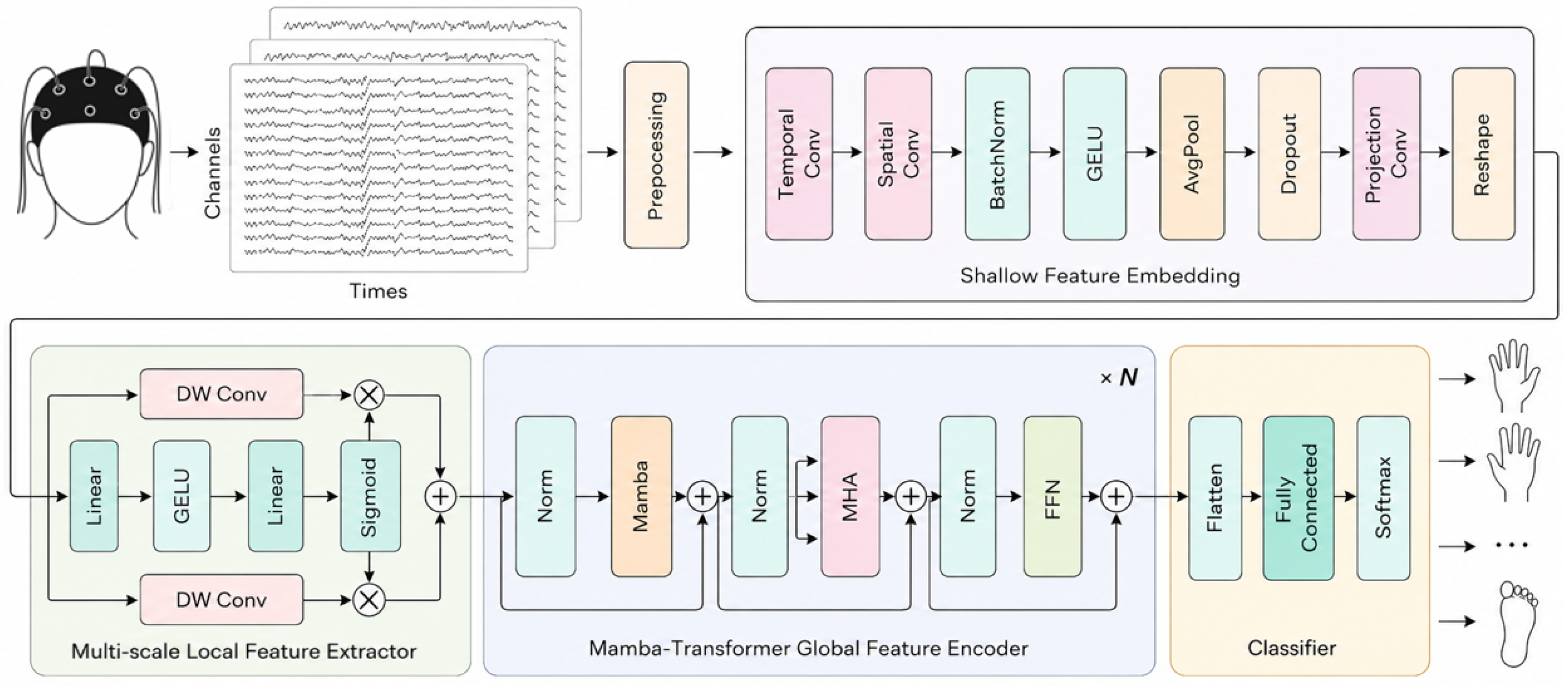
To address the limitations of existing MI-EEG decoding models, we propose a novel deep learning framework that integrates hierarchical feature modeling at both local and global scales. As illustrated in Figure 1, the proposed model consists of three key components: shallow feature embedding (SFE), a multi-scale local feature extractor (MSLFE), and a Mamba–transformer global feature encoder (MTGFE), followed by a classifier.

Given a raw EEG trial ${\mathbf{x}}_i\in {\mathbb{R}}^{C\times T}$, where C and T denote the number of channels and time points, respectively, the SFE module first extracts shallow spatiotemporal features. The MSLFE module then captures local patterns at multiple temporal scales using convolution kernels of different sizes. The MTGFE module further models global contextual dependencies by combining Mamba with multi-head attention (MHA). Finally, the learned features are aggregated and fed into a classifier for prediction.

The overall training procedure of HMT-Net is summarized in Algorithm 1. Given the standardized EEG training set, each mini-batch is first dynamically augmented and then sequentially processed by the SFE, MSLFE, MTGFE, and classifier modules. The network parameters are updated by minimizing the cross-entropy loss.

Algorithm 1: Training procedure of HMT-Net

3.3. Preprocessing

Each raw EEG trial is represented as a multi-channel temporal signal. To reduce the influence of data fluctuation and non-stationarity, we apply a Z-score standardization to the raw EEG signals, which is defined as

$${\mathbf{x}}_o={\displaystyle \frac{{\mathbf{x}}_i-\mu }{\sigma }},$$

(1)

where ${\mathbf{x}}_i$ and ${\mathbf{x}}_o$ denote the input and normalized EEG signals, respectively, and $\mu$ and $\sigma$ represent the mean and standard deviation computed from the training data. The same statistics are applied to normalize the test data.

3.4. Shallow Feature Embedding (SFE)

Inspired by prior EEG convolutional models [11,12], we design the shallow feature embedding (SFE) module to extract low-level spatiotemporal representations from raw EEG signals, as summarized in

Table 1. Network architecture of the shallow feature embedding (SFE) module.

Layer	In	Out	Kernel	Stride	Padding
Temporal Conv	1	k	$(1,25)$	$(1,1)$	$(0,0)$
Spatial Conv	k	k	$(c,1)$	$(1,1)$	$(0,0)$
BatchNorm	k	k	–	–	–
GELU	k	k	–	–	–
Avg Pooling	k	k	$(1,75)$	$(1,15)$	$(0,0)$
Dropout	k	k	–	–	–
Projection Conv	k	k	$(1,1)$	$(1,1)$	$(0,0)$
Rearrange	$(k,1,p)\to (p,k)$

. Specifically, the convolutional operations are decomposed into temporal and spatial convolutions. The first layer applies k kernels of size $(1,25)$ with a stride of $(1,1)$ along the temporal dimension to capture short-term temporal dynamics, while the second layer employs k kernels of size $(C,1)$ with a stride of $(1,1)$ to model inter-channel correlations and spatial dependencies, where C denotes the number of electrode channels. Subsequently, batch normalization is adopted to stabilize the training process, followed by a GELU activation function to introduce nonlinearity. An average pooling layer with a kernel size of $(1,75)$ and a stride of $(1,15)$ is then applied along the temporal dimension to reduce temporal redundancy and computational complexity, and a dropout layer is further introduced to alleviate overfitting. After feature extraction, a $1\times 1$ convolution is utilized as a channel projection to refine feature representation. Finally, the resulting feature maps are rearranged as ${\mathbf{F}}_{\mathrm{SFE}}\in {\mathbb{R}}^{p\times k}$, where p denotes the number of temporal positions and k denotes the number of feature channels. Subsequently, the feature maps are then fed into the subsequent MSLFE module. In our experiments, we set $k=40$ to balance representational capacity and computational efficiency.

3.5. Multi-Scale Local Feature Extractor (MSLFE)

Considering that motor imagery EEG signals exhibit diverse temporal dynamics across different frequency bands and time scales, such as alpha-band rhythms (8–12 Hz) and beta-band rhythms (12–30 Hz), we design a multi-scale local feature extractor (MSLFE) module to capture such multi-scale temporal characteristics. Specifically, as illustrated in Figure 1, two parallel depthwise convolution branches with different kernel sizes are applied to the feature maps ${\mathbf{F}}_{\mathrm{SFE}}$. For each temporal convolution branch, same zero padding is applied along the temporal dimension to preserve the sequence length. For the branch with kernel size $r_i$, the depthwise temporal convolution is formulated as

$${\mathbf{F}}_{r_i}(m,j)={\displaystyle \sum _{\tau =0}^{r_i-1}}{\mathbf{W}}_{r_i}^j\left(\tau \right)·{\mathbf{F}}_{\mathrm{SFE}}(m-\tau ,j),i\in \{1,2\},$$

(2)

where ${\mathbf{W}}_{r_i}^j$ denotes the depthwise convolution kernel of the j-th feature channel in the i-th branch. Since depthwise convolution is performed independently for each feature channel, the two branches extract local temporal patterns at different receptive fields while preserving channel-specific information.

Subsequently, a channel attention gate is introduced to adaptively recalibrate the feature representations from different branches. The attention weights are generated from the input feature maps through global average pooling and two linear transformations:

$${\mathbf{w}}_{gate}=\sigma \left({\mathrm{Linear}}_2\left(\mathrm{GELU}\left({\mathrm{Linear}}_1\left(\mathrm{GAP}\left({\mathbf{F}}_{\mathrm{SFE}}\right)\right)\right)\right)\right),$$

(3)

where $\mathrm{GAP}(·)$ denotes global average pooling, $\sigma (·)$ is the sigmoid function, and $\mathbf{w}\in {\mathbb{R}}^k$ represents the channel-wise attention weights.

The attention weights are then used to gate the multi-scale branch features through element-wise multiplication, and the final MSLFE representation is obtained by

$${\mathbf{F}}_{\mathrm{MSLFE}}={\mathbf{w}}_{gate}\odot {\mathbf{F}}_{r_1}+(1-{\mathbf{w}}_{gate})\odot {\mathbf{F}}_{r_2},$$

(4)

where ⊙ denotes element-wise multiplication. In this way, the MSLFE module adaptively integrates local temporal features from different convolutional scales. The obtained feature representation ${\mathbf{F}}_{\mathrm{MSLFE}}$ is subsequently fed into the MTGFE module for global dependency modeling.

3.6. Mamba–Transformer Global Feature Encoder (MTGFE)

Although convolutional layers can effectively extract local temporal features, they are limited in capturing long-range dependencies and global contextual information in EEG signals. To address this limitation, we design a Mamba–transformer global feature encoder (MTGFE) to further enhance global feature representation. The MTGFE module integrates Mamba with multi-head attention (MHA) to jointly model sequential dependencies and global temporal interactions in the extracted EEG features. Specifically, the Mamba module provides efficient sequence modeling and captures long-range temporal dynamics through state-space representations, while the MHA module explicitly models pairwise interactions among different temporal positions. In this way, Mamba and MHA provide complementary modeling capabilities: Mamba emphasizes efficient temporal state evolution, whereas MHA enhances global interaction modeling across the feature sequence. It consists of three key components: a Mamba module, an MHA module, and a feed-forward network (FFN).

Before feature modeling, sinusoidal positional encoding (PE) is first applied to the input feature maps to preserve temporal order information. Specifically, for a given position $pos$ and embedding dimension i, it is defined as

$$\begin{array}{cc}\hfill \mathrm{PE}(pos,2i)& =sin\left({\displaystyle \frac{pos}{10,{000}^{2i/d}}}\right),\hfill \\ \hfill \mathrm{PE}(pos,2i+1)& =cos\left({\displaystyle \frac{pos}{10,{000}^{2i/d}}}\right),\hfill \end{array}$$

(5)

where d denotes the embedding dimension.

3.6.1. Mamba

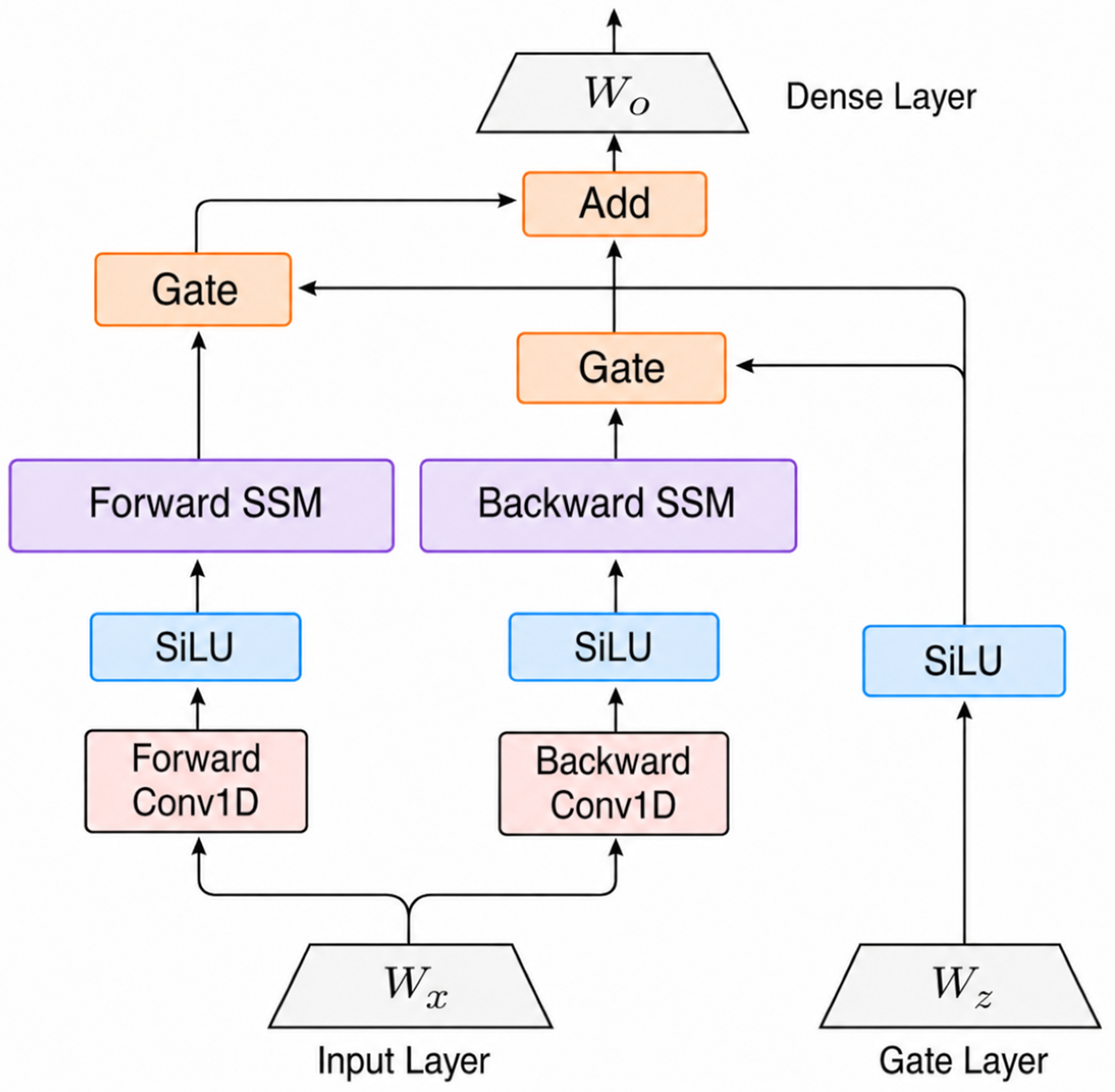
Since offline MI-EEG classification is a non-causal task, the representation of the current EEG state can benefit from both preceding waveform patterns and subsequent temporal variations. Therefore, the Mamba module is adopted to efficiently model long-range dependencies in EEG sequences from bidirectional temporal contexts, as illustrated in Figure 2.

Given the input feature maps, layer normalization is first applied to obtain the normalized input sequence ${\mathbf{X}}_{in}$. Then, ${\mathbf{X}}_{in}$ is projected into two parallel branches through the learnable linear projection matrices ${\mathbf{W}}_x$ and ${\mathbf{W}}_z$. The main branch is used for sequence modeling, while the other branch generates the gating signal:

$${\mathbf{X}}_{conv}=\mathrm{SiLU}\left(\mathrm{Conv}1\mathrm{D}\left({\mathbf{X}}_{in}{\mathbf{W}}_x\right)\right),$$

(6)

$${\mathbf{Z}}_{gate}=\mathrm{SiLU}\left({\mathbf{X}}_{in}{\mathbf{W}}_z\right),$$

(7)

where $\mathrm{Conv}1\mathrm{D}(·)$ denotes the temporal convolution, and $\mathrm{SiLU}(·)$ is the activation function. The temporal convolution in ${\mathbf{X}}_{conv}$ captures local temporal dependencies before the features are passed into the SSM, providing locally contextualized representations for subsequent state-space sequence modeling and reducing the sensitivity to high-frequency artifacts such as electromyography (EMG) interference. Meanwhile, ${\mathbf{Z}}_{gate}$ is used to adaptively modulate the SSM output.

The SSM branch is formulated from a continuous-time linear time-invariant (LTI) system, which describes the evolution of a latent state driven by the input sequence:

$$\dot{\mathbf{h}}\left(t\right)=\mathbf{A}\mathbf{h}\left(t\right)+\mathbf{B}\mathbf{x}\left(t\right),\mathbf{y}\left(t\right)=\mathbf{C}\mathbf{h}\left(t\right)+\mathbf{D}\mathbf{x}\left(t\right),$$

(8)

where $\mathbf{x}\left(t\right)\in {\mathbb{R}}^d$ denotes the input signal at time t, $\mathbf{h}\left(t\right)\in {\mathbb{R}}^{d_s}$ represents the latent state, and $\mathbf{y}\left(t\right)\in {\mathbb{R}}^d$ is the output response. The matrix $\mathbf{A}\in {\mathbb{R}}^{d_s\times d_s}$ is the state transition matrix that governs the temporal evolution of the latent state. The matrix $\mathbf{B}\in {\mathbb{R}}^{d_s\times d}$ projects the input signal into the state space, while $\mathbf{C}\in {\mathbb{R}}^{d\times d_s}$ maps the latent state back to the output space. In addition, $\mathbf{D}\in {\mathbb{R}}^{d\times d}$ denotes the direct input-to-output projection. Here, d and $d_s$ denote the feature dimension and the state dimension, respectively. Different from conventional SSMs with fixed parameters, Mamba introduces a selective mechanism by making part of the state-space parameters input-dependent. Specifically, the input-to-state matrix ${\mathbf{B}}_t$ and the state-to-output matrix ${\mathbf{C}}_t$ are dynamically generated from ${\mathbf{X}}_{conv}\left(t\right)$, while the discretization step is obtained as ${\Delta }_t=\mathrm{Softplus}\left({\mathbf{X}}_{conv}\left(t\right){\mathbf{W}}_{\Delta }\right)$. With the zero-order hold (ZOH) discretization, ${\Delta }_t$ is used to convert the continuous-time parameters into input-dependent discrete parameters, such as ${\overline{\mathbf{A}}}_t=exp\left({\Delta }_t\mathbf{A}\right)$ and ${\overline{\mathbf{B}}}_t$. This input-dependent design enables the SSM to adjust the state update rate according to the current EEG feature. After ZOH discretization, the continuous-time latent state $\mathbf{h}\left(t\right)$ is converted into the discrete sequence representation ${\mathbf{h}}_t$. The discretized recurrent update is then written as

$${\mathbf{h}}_t={\overline{\mathbf{A}}}_t{\mathbf{h}}_{t-1}+{\overline{\mathbf{B}}}_t{\mathbf{X}}_{conv}\left(t\right),{\mathbf{Y}}_{ssm}\left(t\right)={\mathbf{C}}_t{\mathbf{h}}_t+\mathbf{D}{\mathbf{X}}_{conv}\left(t\right),$$

(9)

where ${\overline{\mathbf{A}}}_t$ and ${\overline{\mathbf{B}}}_t$ denote the input-dependent discretized state transition matrix and input projection matrix, respectively.

To explicitly capture contextual information from both temporal directions, the selective SSM is applied in a bidirectional manner. The forward branch processes the sequence in its original temporal order, while the backward branch models the reversed sequence:

$${\mathbf{O}}_f={\mathrm{SSM}}_f\left({\mathbf{X}}_{conv}\right),{\mathbf{O}}_b=\mathrm{Flip}\left({\mathrm{SSM}}_b\left(\mathrm{Flip}\left({\mathbf{X}}_{conv}\right)\right)\right),$$

(10)

where $\mathrm{Flip}(·)$ denotes reversing the sequence along the temporal dimension. The forward ${\mathrm{SSM}}_f$ captures dependencies from past to future, whereas the backward ${\mathrm{SSM}}_b$ incorporates contextual information from future to past. The gating signal ${\mathbf{Z}}_{gate}$ is computed once from the input projection branch and shared by the forward and backward SSM branches. Then, the bidirectional SSM outputs are modulated by the shared gating signal and aggregated:

$${\mathbf{Y}}_{out}={\mathbf{W}}_o\left(\left({\mathbf{O}}_f\odot {\mathbf{Z}}_{gate}\right)+\left({\mathbf{O}}_b\odot {\mathbf{Z}}_{gate}\right)\right),$$

(11)

where ⊙ denotes element-wise multiplication, and ${\mathbf{W}}_o$ is the dense output projection layer. The resulting representation ${\mathbf{Y}}_{out}$ is used as the output of the Mamba module.

3.6.2. Multi-Head Attention (MHA)

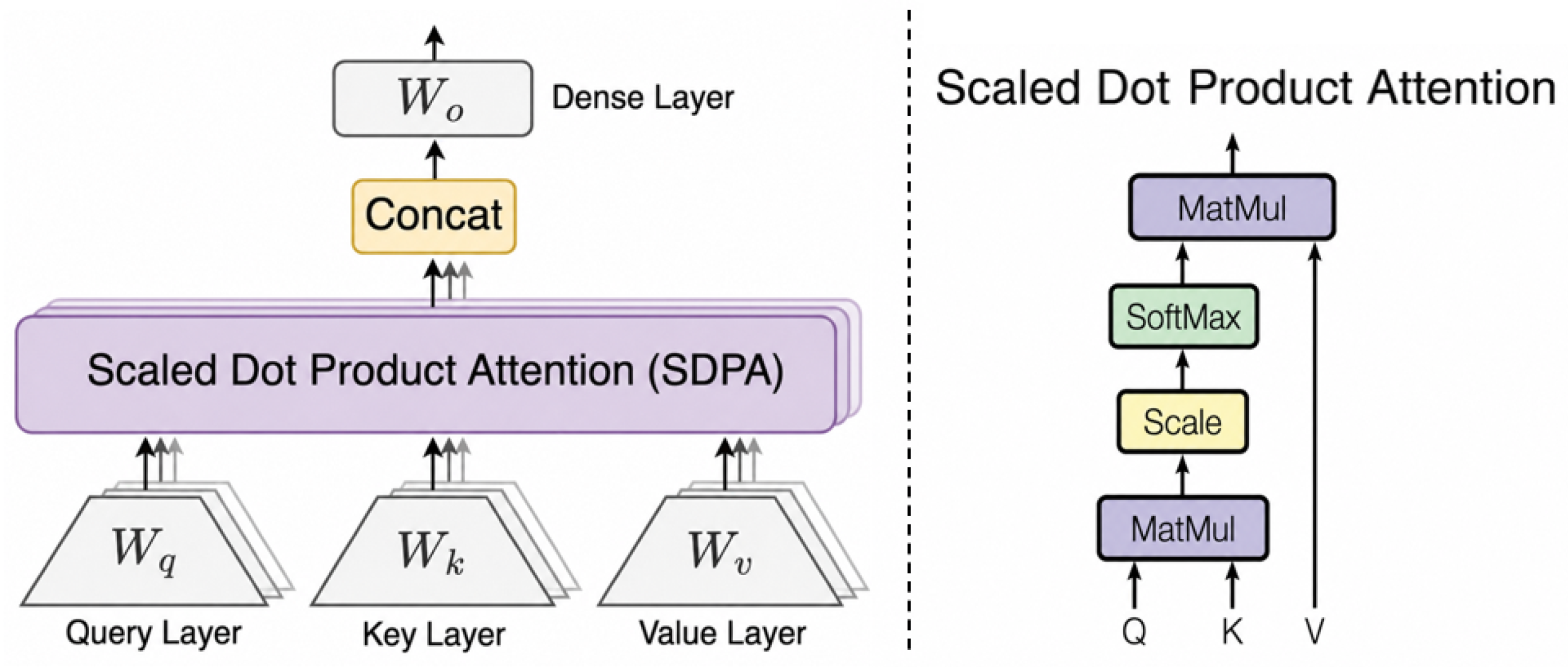
To further enhance global dependency modeling, a multi-head attention (MHA) mechanism is employed, as illustrated in Figure 3.

The input features are first linearly projected to obtain the query ($\mathbf{Q}$), key ($\mathbf{K}$), and value ($\mathbf{V}$) representations. Dot product similarity is computed between $\mathbf{Q}$ and $\mathbf{K}$ to measure the correlation between different tokens. A scaling factor is introduced to stabilize the gradients, followed by a softmax operation to obtain the attention weights. The weighted sum over the value $\mathbf{V}$ produces the attention output, which can be formulated as

$$\mathrm{Attention}(\mathbf{Q},\mathbf{K},\mathbf{V})=\mathrm{Softmax}\left({\displaystyle \frac{\mathbf{Q}{\mathbf{K}}^{\top }}{\sqrt{d_k}}}\right)\mathbf{V},$$

(12)

where $d_k$ denotes the dimension of the key vectors.

Subsequently, a multi-head strategy is adopted to enhance representation diversity [28]. The feature representations are evenly divided into h subspaces and processed by the attention mechanism in parallel. The outputs of all heads are then concatenated and linearly projected to form the final output, which can be expressed as

$$\begin{array}{cc}\hfill \mathrm{MHA}(\mathbf{Q},\mathbf{K},\mathbf{V})& =\mathrm{Concat}({\mathrm{head}}_1,\dots ,{\mathrm{head}}_h){\mathbf{W}}_o,\hfill \\ \hfill {\mathrm{head}}_i& =\mathrm{Attention}({\mathbf{Q}}_i,{\mathbf{K}}_i,{\mathbf{V}}_i),\hfill \end{array}$$

(13)

where ${\mathbf{W}}_o$ is a learnable projection matrix, and ${\mathbf{Q}}_i$, ${\mathbf{K}}_i$, and ${\mathbf{V}}_i$ denote the query, key, and value of the i-th head, respectively.

3.6.3. Feed-Forward Network (FFN)

After the multi-head attention module, a feed-forward network (FFN) is employed to further refine the feature representations. The FFN consists of two linear transformations with a nonlinear activation function in between, and is applied independently to each position, which can be formulated as

$$\mathrm{FFN}\left(\mathbf{x}\right)=\mathrm{GELU}(\mathbf{x}{\mathbf{W}}_1+{\mathbf{b}}_1){\mathbf{W}}_2+{\mathbf{b}}_2.$$

(14)

Furthermore, residual connections are applied to the Mamba, MHA, and FFN modules to ensure stable training.

3.7. Classifier

Finally, the extracted features are flattened and fed into a fully connected (FC) layer, followed by a softmax function to produce the final predictions. The cross-entropy loss is adopted for model optimization, which is defined as

$$\mathcal{L}=-{\displaystyle \frac{1}{N_b}}{\displaystyle \sum _{i=1}^{N_b}}{\displaystyle \sum _{c=1}^M}{y}_{i,c}log\left({\widehat{y}}_{i,c}\right),$$

(15)

where M denotes the number of classes, y and $\widehat{y}$ represent the ground truth and predicted probabilities, respectively, and $N_b$ is the batch size.

4. Experiments

4.1. Datasets

To comprehensively evaluate the proposed method, experiments are conducted on three widely used motor imagery electroencephalography (MI-EEG) datasets: BCI Competition IV-2a (BCI-IV-2a), BCI Competition IV-2b (BCI-IV-2b) [29], and the High Gamma Dataset (HGD) [12]. A summary of their key characteristics is provided in

Table 2. Summary of the three MI-EEG datasets.

Dataset	Subjects	Channels	Sampling Rate	Duration	Trials	Task Types
BCI-IV-2a	9	22	250 Hz	4 s	5184	left hand/right hand/feet/tongue
BCI-IV-2b	9	3	250 Hz	4 s	6520	left hand/right hand
HGD	14	128	500 Hz	4 s	13,440	left hand/right hand/feet/rest

.

4.1.1. BCI-IV-2a

BCI-IV-2a is a four-class MI dataset involving left hand, right hand, both feet, and tongue imagery tasks from nine subjects. EEG signals were recorded using 22 channels at a sampling rate of 250 Hz, with each trial lasting 4 s. The original signals were band-pass filtered between 0.5 and 100 Hz, with a 50 Hz notch filter enabled. The dataset consists of two sessions recorded on different days, including a training session and an evaluation session. Following the standard protocol, the training session is used for model fitting, while the evaluation session is used for testing. The dataset is available at https://www.bbci.de/competition/iv/ (accessed on 1 May 2026).

4.1.2. BCI-IV-2b

BCI-IV-2b is a two-class MI dataset (left vs. right hand) collected from nine subjects. EEG signals were acquired using three bipolar channels (C3, Cz, and C4) at 250 Hz, with each trial lasting 4 s. The original signals were band-pass filtered between 0.5 and 100 Hz, with a 50 Hz notch filter enabled. Each subject participated in five sessions, including both non-feedback and feedback recordings. In our experiments, the first three sessions are used for training, and the remaining two sessions are used for testing. The dataset is available at: https://www.bbci.de/competition/iv/ (accessed on 1 May 2026).

4.1.3. HGD

HGD is a large-scale four-class MI dataset (left hand, right hand, both feet, and rest) collected from 14 subjects using 128 EEG channels at a sampling rate of 500 Hz. Following the standard setting of this dataset, 44 sensors covering the motor cortex are used for model training and evaluation. The EEG signals are high-pass filtered at 4 Hz, and trials with amplitudes exceeding 800 μV are removed to exclude extreme high-amplitude artifacts. To ensure consistency across datasets, all signals are downsampled to 250 Hz, and the 0–4 s segment after cue onset is extracted as model input. Compared to the BCI datasets, HGD provides higher spatial resolution and a larger number of trials, offering a more challenging and comprehensive evaluation setting. The dataset is available at https://braindecode.org/stable/generated/braindecode.datasets.HGD.html (accessed on 1 May 2026).

4.2. Data Augmentation

Due to the limited amount of EEG data and the high cost of acquisition, deep learning models are prone to overfitting when trained on MI-EEG datasets. To alleviate this issue, we adopt a data augmentation strategy based on segmentation and recombination (S&R) in the time domain [30,31]. Specifically, EEG trials belonging to the same class are divided into several segments of the same length along the temporal dimension. New samples are then generated by randomly selecting and concatenating segments from different trials of the same class while preserving their original temporal order. This process maintains the inherent temporal structure of EEG signals and introduces additional variability, thereby improving the generalization ability of the model.

4.3. Baseline Comparison

We compare the proposed model with several representative MI-EEG decoding approaches, including ShallowConvNet [12], DeepConvNet [12], EEGNet [11], FBCNet [24], EEGConformer [14], ATCNet [15], TMSA-Net [17] and FA-STTM [32]. For fair comparison, all reproduced baseline methods are evaluated using the same preprocessing pipeline, training and test set partition, and evaluation metrics as HMT-Net. The training settings for each model, including the number of training epochs, batch size, optimizer, learning rate, and other hyperparameters, follow the official implementation procedures or the original papers whenever available. All reproduced models are trained and evaluated under the same experimental environment. For FA-STTM, since its official implementation is not publicly available, we report the results from the original paper for comparison.

4.3.1. ShallowConvNet

ShallowConvNet is a shallow convolutional network capturing bandpower features through temporal and spatial convolutions, inspired by FBCSP [33] principles.

4.3.2. DeepConvNet

DeepConvNet is a deep convolutional network designed to learn hierarchical features from raw EEG, with a spatiotemporal convolution block followed by multiple convolutional layers with max-pooling for end-to-end decoding.

4.3.3. EEGNet

EEGNet is a compact architecture utilizing depthwise and separable convolutions to efficiently model temporal and spatial dependencies with minimal computational cost.

4.3.4. FBCNet

FBCNet leverages filter-bank convolution to extract frequency-specific features, decomposing EEG into multi-view representations for efficient MI decoding with a small parameter footprint.

4.3.5. EEGConformer

EEGConformer integrates convolutional modules with transformer-based attention to capture local spatiotemporal features and global dependencies, improving accuracy and robustness in MI-EEG decoding.

4.3.6. ATCNet

ATCNet combines self-attention with a temporal convolutional network (TCN) [34] to model dynamic temporal dependencies, effectively identifying discriminative time segments in motor imagery tasks.

4.3.7. TMSA-Net

TMSA-Net uses multi-scale attention to simultaneously capture fine-grained local features and long-range global dependencies, enhancing decoding performance on non-stationary EEG signals.

4.3.8. FA-STTM

FA-STTM is a frequency-aware spatiotemporal transformer for MI-EEG decoding, combining wavelet-based spatial and channel attention with a Mamba–transformer module to capture global dependencies and a Kolmogorov–Arnold network (KAN) [35] for enhanced representation.

4.4. Training Configuration

All experiments are implemented using PyTorch 2.5.1 and conducted on a workstation equipped with an NVIDIA RTX 4090 GPU. The proposed model is evaluated under both subject-dependent and subject-independent settings. In the subject-dependent setting, models are trained and tested separately for each subject. In the subject-independent setting, a Leave-One-Subject-Out (LOSO) strategy is adopted, where one subject is used for testing while the remaining subjects are used for training. The hyperparameters used in this work are summarized in

Table 3. Parameter settings of the proposed model.

Parameter	BCI-IV-2a	BCI-IV-2b	HGD
Optimizer	AdamW	AdamW	AdamW
Learning Rate	$5\times {10}^{-4}$	$5\times {10}^{-4}$	$5\times {10}^{-4}$
Batch Size	72	72	72
Epochs	500	500	500
Convolution Kernels	$1,3$	$5,7$	$5,7$
MHA Heads	8	8	8
MTGFE Blocks	1	1	1
Embedding Dimension	40	40	40
FFN Dimension	80	80	80
State Dimension	8	8	8
Dropout	0.1	0.1	0.1

. AdamW is adopted as the optimizer with a fixed learning rate of $5\times {10}^{-4}$ and the default weight decay of 0.01. No learning rate scheduler is used in our experiments. For subject-dependent evaluations, the number of training epochs is set to 500 as listed in the table. For subject-independent evaluations, the number of training epochs is reduced to 200, since training is performed on data from multiple subjects, resulting in a substantially larger number of training samples. Inspired by [36], this setting is sufficient to ensure model convergence while avoiding excessive training time and the risk of overfitting. For S&R data augmentation, the number of temporal segments is set to $N_s=8$, where each segment corresponds to a duration of 0.5 s.

To provide a comprehensive evaluation, we employ multiple widely used metrics, including accuracy, precision, recall, F1-score, and Cohen’s kappa [12,37,38]. Accuracy reflects the overall proportion of correct predictions, while precision and recall measure the correctness of positive predictions and the ability to identify true positive samples, respectively. The F1-score, as the harmonic mean of precision and recall, provides a balanced evaluation. Among these metrics, classification accuracy (ACC) and Cohen’s kappa coefficient are adopted as the primary evaluation criteria. The ACC is defined as

$$\mathrm{ACC}={\displaystyle \frac{TP+TN}{TP+TN+FP+FN}},$$

(16)

and the kappa coefficient is given by

$$\kappa ={\displaystyle \frac{p_o-p_e}{1-p_e}},$$

(17)

where $TP$, $TN$, $FP$, and $FN$ denote true positives, true negatives, false positives, and false negatives, respectively; $p_o$ represents the observed accuracy and $p_e$ denotes the expected accuracy by random chance.

5. Results

In this section, we evaluate the proposed model on three benchmark MI-EEG datasets under both subject-dependent and subject-independent settings. The classification performance is first compared with several representative state-of-the-art (SOTA) methods to demonstrate the effectiveness of the proposed approach. We then conduct ablation studies to investigate the contribution of key components in the model, along with an analysis of important design choices. Finally, a series of visualization experiments are presented to provide insights into the interpretability of the learned representations.

5.1. Subject-Dependent Classification

To comprehensively evaluate the effectiveness of the proposed method, we first analyze the subject-dependent classification results on three benchmark datasets.

The classification performance on the BCI-IV-2a dataset is reported in

Table 4. Subject-dependent classification performance on the BCI-IV-2a dataset.

Methods	A01	A02	A03	A04	A05	A06	A07	A08	A09	Avg ± Std (%)	Kappa	P
ShallowConvNet [12]	71.88	52.78	84.03	59.03	61.46	52.43	78.47	79.17	72.22	67.94 ± 11.84	0.57	0.0001
DeepConvNet [12]	67.71	51.39	77.78	63.54	73.26	48.26	72.92	71.53	74.65	66.78 ± 10.47	0.56	0.0001
EEGNet [11]	73.26	62.50	91.67	64.93	76.39	57.96	72.92	77.08	75.00	72.42 ± 9.86	0.63	0.0035
FBCNet [24]	88.19	66.32	93.75	76.39	70.83	56.94	94.79	82.29	81.94	79.05 ± 12.71	0.72	0.0746
EEGConformer [14]	86.11	52.08	94.79	75.00	78.47	63.89	89.24	88.54	82.29	78.94 ± 13.58	0.72	0.0064
ATCNet [15]	80.90	61.81	92.36	78.82	74.65	68.40	78.82	84.03	80.90	77.47 ± 9.38	0.70	0.0060
TMSA-Net [17]	83.68	58.33	93.06	80.90	76.04	64.24	89.93	88.19	84.38	79.86 ± 11.74	0.73	0.0040
FA-STTM [32]	85.76	70.14	94.09	86.80	82.29	69.09	85.76	86.45	85.76	82.90 ± 8.15	0.77	0.5476
HMT-Net (Ours)	88.19	59.38	95.14	86.46	81.60	75.00	95.49	88.89	86.46	84.07 ± 11.20	0.79	–

. It can be observed that the proposed HMT-Net achieves the best overall performance, with an average accuracy of 84.07% and a kappa value of 0.79. Compared with conventional CNN-based methods such as ShallowConvNet, DeepConvNet, and EEGNet, HMT-Net achieves statistically significant improvements, indicating the advantage of more expressive feature representations. Compared with advanced architectures, including EEGConformer, ATCNet, and TMSA-Net, our method also demonstrates statistically significant performance gains. Although FBCNet and FA-STTM achieve strong results on certain subjects, the improvements of HMT-Net over these two methods are not statistically significant. Nevertheless, HMT-Net maintains the highest average accuracy and kappa value, suggesting better overall robustness and demonstrating the effectiveness of jointly modeling local and global dependencies.

The results on the BCI-IV-2b dataset are presented in

Table 5. Subject-dependent classification performance on the BCI-IV-2b dataset.

Methods	B01	B02	B03	B04	B05	B06	B07	B08	B09	Avg ± Std (%)	Kappa	P
ShallowConvNet [12]	75.94	67.14	76.56	97.19	95.00	88.44	87.19	93.13	86.56	85.24 ± 10.03	0.70	0.0035
DeepConvNet [12]	74.38	75.71	86.25	97.81	96.25	85.00	91.25	95.94	86.56	87.08 ± 8.57	0.75	0.0388
EEGNet [11]	73.13	72.50	86.88	97.50	95.31	84.69	91.25	96.25	84.06	86.84 ± 9.35	0.74	0.0216
FBCNet [24]	80.94	57.14	57.50	91.88	93.44	91.56	80.00	91.25	91.56	82.29 ± 15.22	0.65	0.0749
EEGConformer [14]	78.75	71.43	86.88	97.81	98.75	87.50	91.56	95.00	91.25	88.77 ± 8.95	0.75	0.2146
ATCNet [15]	76.56	72.86	87.19	98.75	95.31	85.94	92.81	95.00	85.31	87.75 ± 8.75	0.76	0.0394
TMSA-Net [17]	77.50	68.21	87.19	98.75	95.94	87.81	93.12	93.44	90.00	88.00 ± 9.62	0.76	0.1260
FA-STTM [32]	77.50	72.50	82.81	98.13	95.62	86.25	93.12	95.31	89.06	87.81 ± 9.35	0.76	0.0233
HMT-Net (Ours)	80.31	76.07	86.56	97.81	98.44	90.00	92.19	95.31	89.69	89.60 ± 7.61	0.79	–

. A similar trend can be observed, where HMT-Net achieves the best average performance with an accuracy of 89.60% and a kappa of 0.79. According to the paired t-test results, HMT-Net significantly outperforms ShallowConvNet, DeepConvNet, EEGNet, ATCNet, and FA-STTM. Compared with FBCNet, EEGConformer, and TMSA-Net, the improvements are positive but not statistically significant, suggesting that the performance gaps among these methods are relatively small on this binary classification dataset. Although several methods achieve competitive results on individual subjects, HMT-Net demonstrates more balanced overall performance and better average generalization capability.

The classification results on the HGD dataset are summarized in

Table 6. Subject-dependent classification performance on the HGD dataset.

Subject	ShallowConvNet [12]	DeepConvNet [12]	EEGNet [11]	FBCNet [24]	EEGConformer [14]	ATCNet [15]	TMSA-Net [17]	HMT-Net (Ours)
H01	95.62	86.88	86.88	92.50	96.25	96.88	95.00	96.88
H02	93.12	95.63	91.25	91.88	95.63	96.88	92.50	95.00
H03	96.88	96.25	96.25	100	100	100	98.75	100
H04	98.12	95.00	93.12	100	98.13	98.75	98.12	99.38
H05	96.88	94.38	95.63	97.50	97.50	98.12	95.63	97.50
H06	94.38	93.13	94.38	96.25	97.50	97.50	97.50	97.50
H07	90.57	88.05	87.42	89.31	92.45	94.34	88.05	94.34
H08	94.38	89.38	93.12	97.50	96.25	96.25	95.00	95.63
H09	96.88	96.25	96.25	88.75	98.13	98.13	95.63	98.13
H10	91.25	88.75	90.00	93.75	92.50	95.00	92.50	92.50
H11	86.25	90.63	78.12	80.63	93.75	88.75	89.38	96.88
H12	96.25	95.00	92.50	95.63	96.88	96.25	96.25	96.25
H13	93.08	89.94	93.71	91.82	95.60	96.23	95.60	95.60
H14	88.12	91.25	78.13	70.63	88.75	89.38	80.63	88.75
Avg ± Std (%)	93.70 ± 3.55	92.18 ± 3.28	90.48 ± 5.98	91.87 ± 7.98	95.66 ± 2.93	95.89 ± 3.24	93.61 ± 4.84	96.02 ± 2.87
Kappa	0.92	0.90	0.87	0.89	0.94	0.95	0.91	0.95
P	0.0056	0.0006	0.0008	0.0281	0.2293	0.8409	0.0069	–

. Since FA-STTM does not report results on this dataset, it is not included in the comparison. It can be seen that HMT-Net achieves the highest average accuracy of 96.02% with a kappa value of 0.95, outperforming all competing methods. The paired t-test results show that HMT-Net achieves statistically significant improvements over ShallowConvNet, DeepConvNet, EEGNet, FBCNet, and TMSA-Net. In contrast, the differences between HMT-Net and EEGConformer or ATCNet are not statistically significant, indicating that these models achieve comparable performance on high-density EEG data. Overall, the proposed method shows consistently strong performance across most subjects, with relatively low variance, further validating its effectiveness in handling high-density EEG data with more complex spatial information.

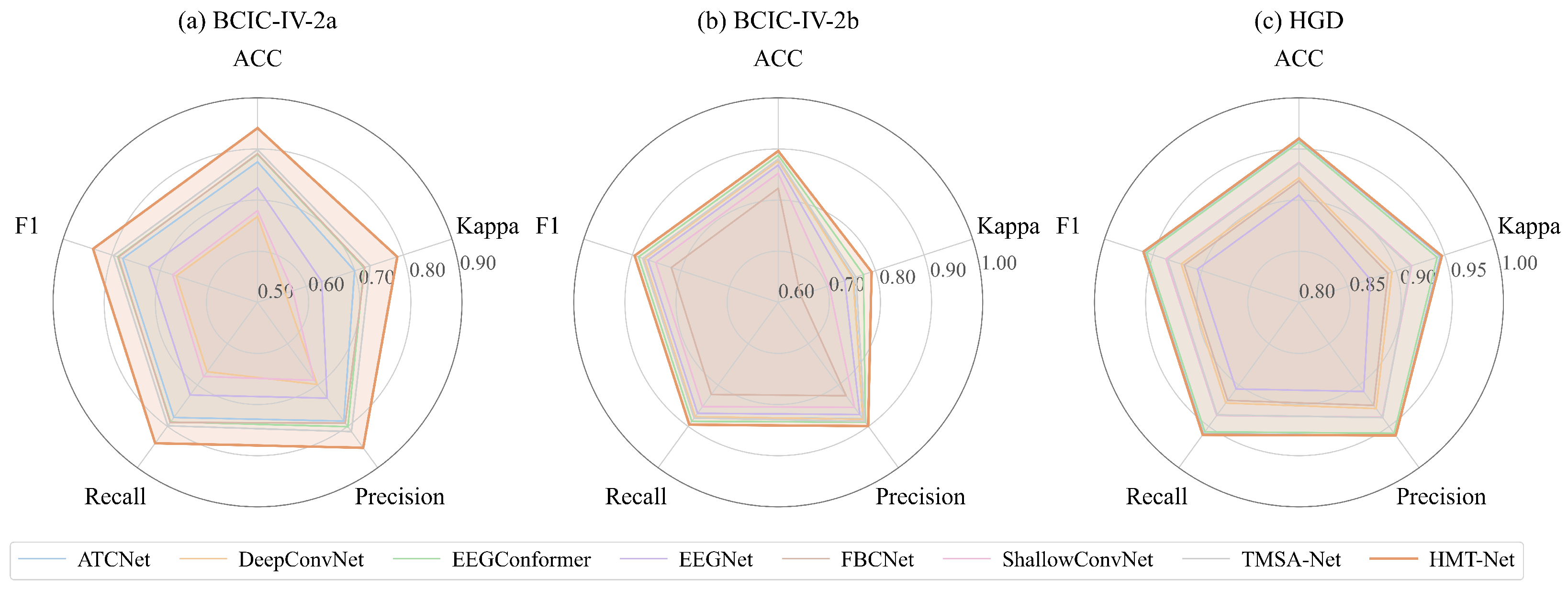
To provide a more intuitive comparison across multiple evaluation metrics, Figure 4 presents radar charts of ACC, kappa, F1-score, recall, and precision on the three datasets. It can be observed that HMT-Net consistently achieves superior performance across all metrics, demonstrating its balanced and robust representation capability.

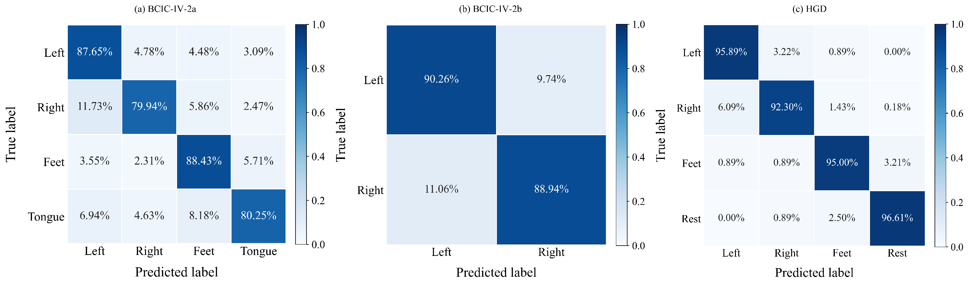
Furthermore, to visually examine the prediction performance, Figure 5 shows the average normalized confusion matrices for HMT-Net on the BCI-IV-2a, BCI-IV-2b, and HGD datasets. Each matrix represents the average prediction distribution across subjects, highlighting the ability of the model to correctly classify each class. It can be seen that the diagonal values are consistently high across all datasets, indicating strong per-class accuracy, while off-diagonal values remain low, reflecting minimal misclassification between classes.

5.2. Subject-Independent Classification

To comprehensively evaluate the effectiveness of the proposed HMT-Net under cross-subject settings, we conducted subject-independent experiments using the Leave-One-Subject-Out (LOSO) protocol on three benchmark datasets, namely BCI-IV-2a, BCI-IV-2b, and HGD. For comparison, we selected representative baseline models, including ATCNet, EEGConformer, TMSA-Net, and FA-STTM. These models were chosen for two main reasons. First, they are widely recognized as state-of-the-art EEG classification architectures. Second, LOSO experiments are computationally expensive, and these models provide reasonable baselines in terms of both performance and training time.

For statistical comparison, paired t-tests across subjects were conducted between HMT-Net and each baseline method, and the corresponding p-values are reported in

Table 7. Subject-independent classification performance under the LOSO setting on the BCI-IV-2a dataset.

Method	ACC	Kappa	F1	Rec.	Prec.	P
EEGConformer [14]	63.66	0.52	0.62	0.64	0.67	0.2537
ATCNet [15]	63.95	0.52	0.64	0.67	0.64	0.5118
TMSA-Net [17]	63.50	0.51	0.63	0.63	0.67	0.3385
FA-STTM [32]	61.13	0.48	–	–	–	0.0424
HMT-Net (Ours)	64.85	0.53	0.64	0.64	0.68	–

,

Table 8. Subject-independent classification performance under the LOSO setting on the BCI-IV-2b dataset.

Method	ACC	Kappa	F1	Rec.	Prec.	P
EEGConformer [14]	78.11	0.56	0.78	0.78	0.79	0.8016
ATCNet [15]	78.27	0.57	0.78	0.78	0.80	0.9773
TMSA-Net [17]	77.52	0.55	0.77	0.78	0.79	0.3351
FA-STTM [32]	77.04	0.54	–	–	–	0.3686
HMT-Net (Ours)	78.30	0.57	0.78	0.80	0.78	–

and

Table 9. Subject-independent classification performance under the LOSO setting on the HGD dataset.

Method	ACC	Kappa	F1	Rec.	Prec.	P
EEGConformer [14]	80.69	0.74	0.80	0.81	0.82	0.0274
ATCNet [15]	78.13	0.71	0.78	0.78	0.80	0.0041
TMSA-Net [17]	73.27	0.64	0.73	0.73	0.78	0.0001
FA-STTM [32]	72.52	0.76	–	–	–	–
HMT-Net (Ours)	83.65	0.78	0.84	0.84	0.85	–

. Each subject was treated as one paired observation, and p < 0.05 indicates a statistically significant difference compared with HMT-Net. Table 7, Table 8 and Table 9 summarize the subject-independent classification results. On the BCI-IV-2a dataset (Table 7), HMT-Net achieves the best overall performance, with an ACC of 64.85% and a kappa value of 0.53. Compared with ATCNet, EEGConformer, and TMSA-Net, HMT-Net obtains positive mean accuracy improvements, although the paired t-test results show that these improvements are not statistically significant. Compared with FA-STTM, HMT-Net achieves a statistically significant improvement ($p=0.0424$), suggesting better cross-subject generalization than the closest Mamba–transformer-based baseline on BCI-IV-2a. Similar trends are observed on the BCI-IV-2b dataset (Table 8), where HMT-Net reaches 78.30% accuracy and 0.57 kappa. Although HMT-Net obtains the highest average accuracy, the differences compared with ATCNet, EEGConformer, TMSA-Net, and FA-STTM are not statistically significant. This result is consistent with the small performance gaps among the compared methods on this binary classification dataset. On the HGD dataset (Table 9), HMT-Net achieves 83.65% ACC and 0.78 kappa, outperforming all baselines and demonstrating superior generalization on high-density EEG. Unlike the results on BCI-IV-2a and BCI-IV-2b, the paired t-test results show that HMT-Net achieves statistically significant improvements over EEGConformer, ATCNet, and TMSA-Net. Since subject-wise FA-STTM results on HGD are unavailable, the paired statistical test is not reported for this comparison. Nevertheless, HMT-Net achieves a substantially higher average ACC than FA-STTM, suggesting stronger cross-subject generalization capability when more training subjects and high-density EEG channels are available.

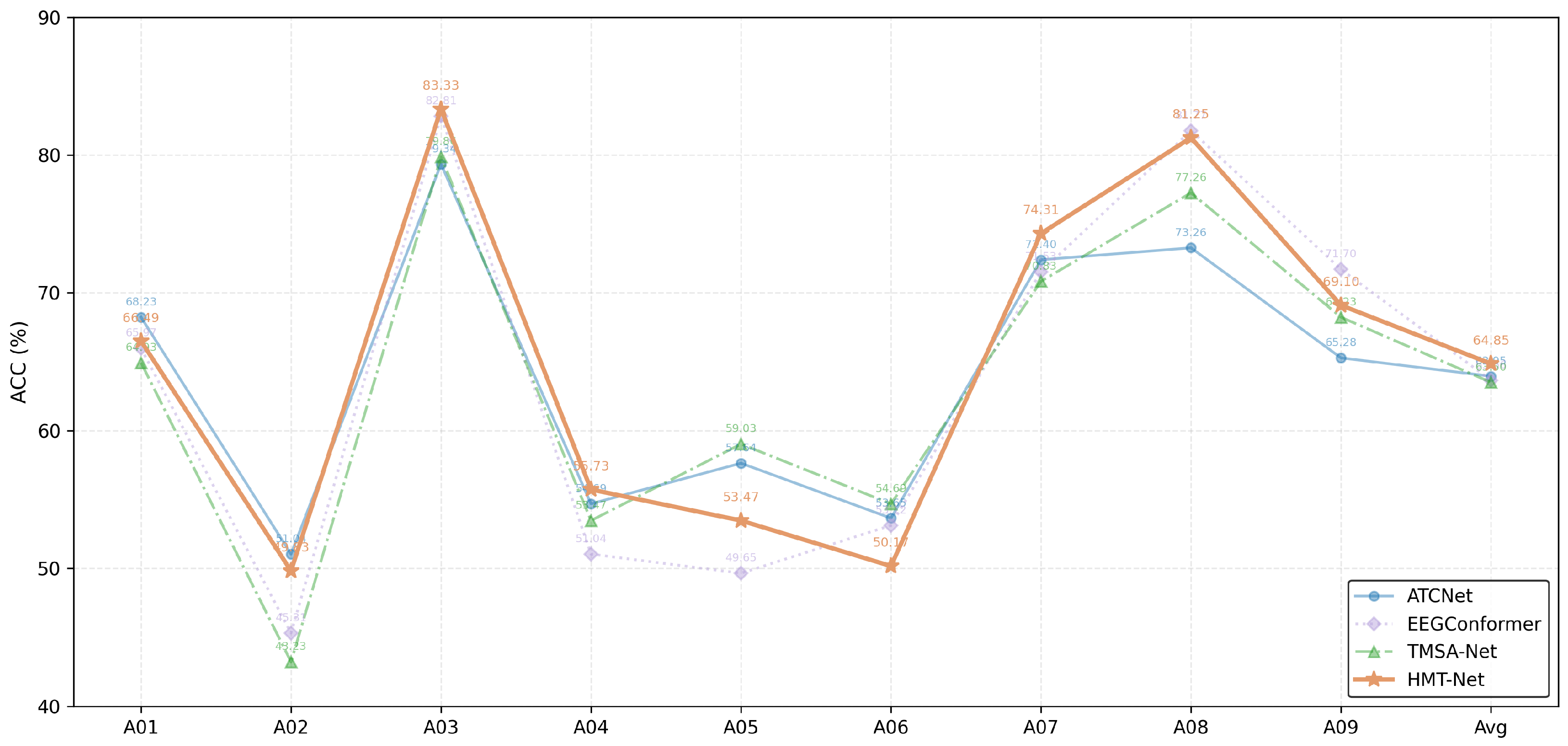
In Figure 6, the accuracy of each subject on the BCI-IV-2a dataset under the LOSO setting is presented. HMT-Net achieves competitive or superior performance across most subjects compared with the baseline methods, indicating its robustness to inter-subject variability. In particular, the average accuracy of HMT-Net is higher than that of the compared methods, demonstrating its overall effectiveness in cross-subject motor imagery EEG classification.

5.3. Ablation Study

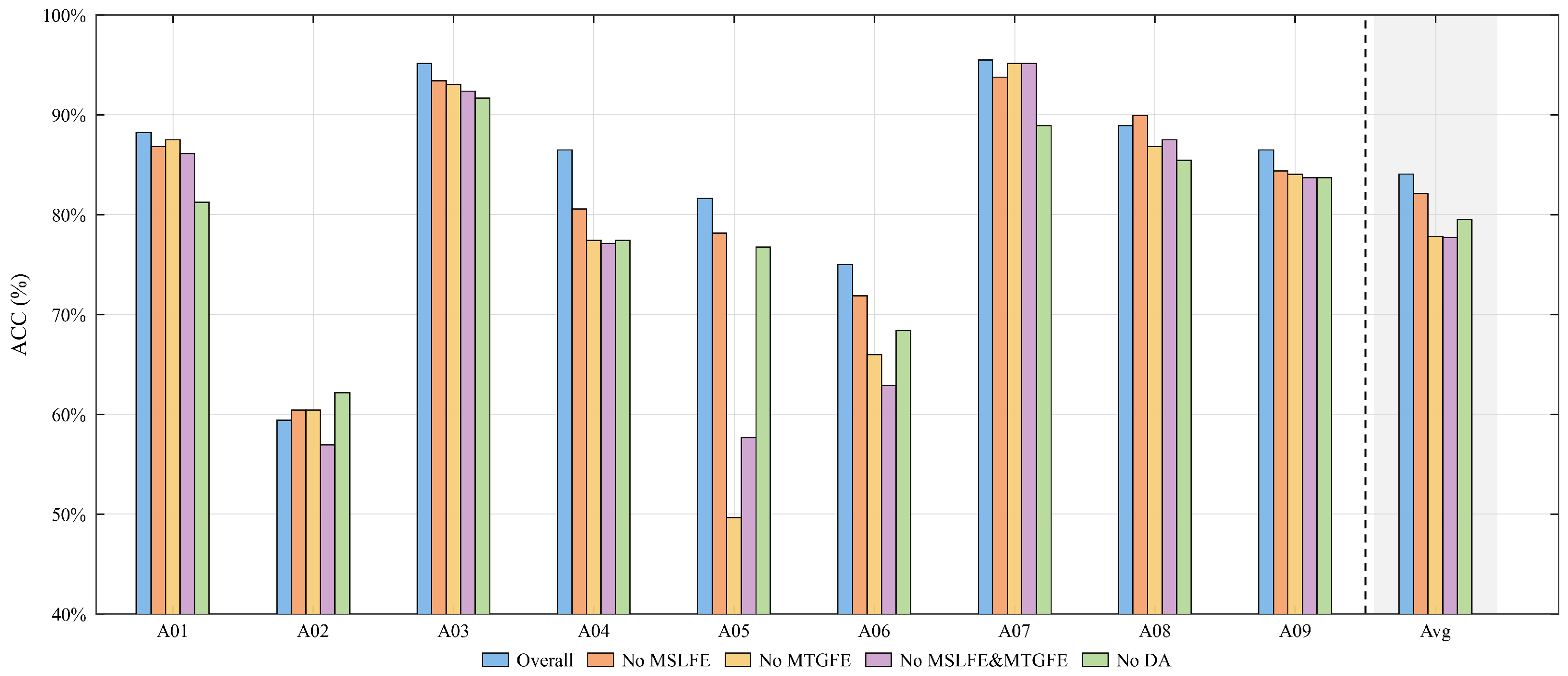
To comprehensively evaluate the contribution of each component in HMT-Net, we perform ablation experiments on three benchmark datasets under the subject-dependent setting. The experiments include two parts. First, we investigate the internal structure of the MTGFE module by comparing three variants, namely Mamba, transformer, and Mamba–transformer. Second, we compare the full model (Overall) with variants where the MSLFE module, the MTGFE module, both modules, or data augmentation (DA) are removed.

For the MTGFE ablation, the FFN module is retained in all variants to provide a consistent feature projection and ensure a fair comparison. In the Mamba variant, only the Mamba sequence modeling module is retained, while the MHA module is removed. In contrast, in the transformer variant, only the MHA-based transformer structure is retained, while the Mamba module is removed. The Mamba–transformer variant retains both modules simultaneously. As shown in

Table 10. Ablation study on MTGFE on BCI-IV-2a, BCI-IV-2b, and HGD.

Dataset	Variant	Mamba	MHA	FFN	ACC ± Std (%)	Kappa
BCI-IV-2a	Mamba	✓	✕	✓	83.26 ± 9.93	0.78
BCI-IV-2a	Transformer	✕	✓	✓	82.33 ± 9.94	0.76
BCI-IV-2a	Mamba-Transformer	✓	✓	✓	84.07 ± 11.20	0.79
BCI-IV-2b	Mamba	✓	✕	✓	88.55 ± 8.04	0.77
BCI-IV-2b	Transformer	✕	✓	✓	89.22 ± 9.04	0.78
BCI-IV-2b	Mamba-Transformer	✓	✓	✓	89.60 ± 7.61	0.79
HGD	Mamba	✓	✕	✓	95.89 ± 2.61	0.95
HGD	Transformer	✕	✓	✓	95.93 ± 2.85	0.95
HGD	Mamba-Transformer	✓	✓	✓	96.02 ± 2.87	0.95

Note: ✓ indicates that the feature is included, while ✕ indicates that it is not.

, the combined Mamba–transformer variant consistently achieves the highest ACC and kappa values across all datasets. The Mamba module is effective in capturing long-range sequence dependencies and temporal dynamics, while the transformer module explicitly models global relationships among temporal positions. Their complementary roles enable the network to exploit both sequential dynamics and global contextual interactions. The reduced performance of either single-module variant demonstrates that neither module alone is sufficient, indicating that both the Mamba and transformer modules are important for robust and discriminative EEG feature representation within MTGFE.

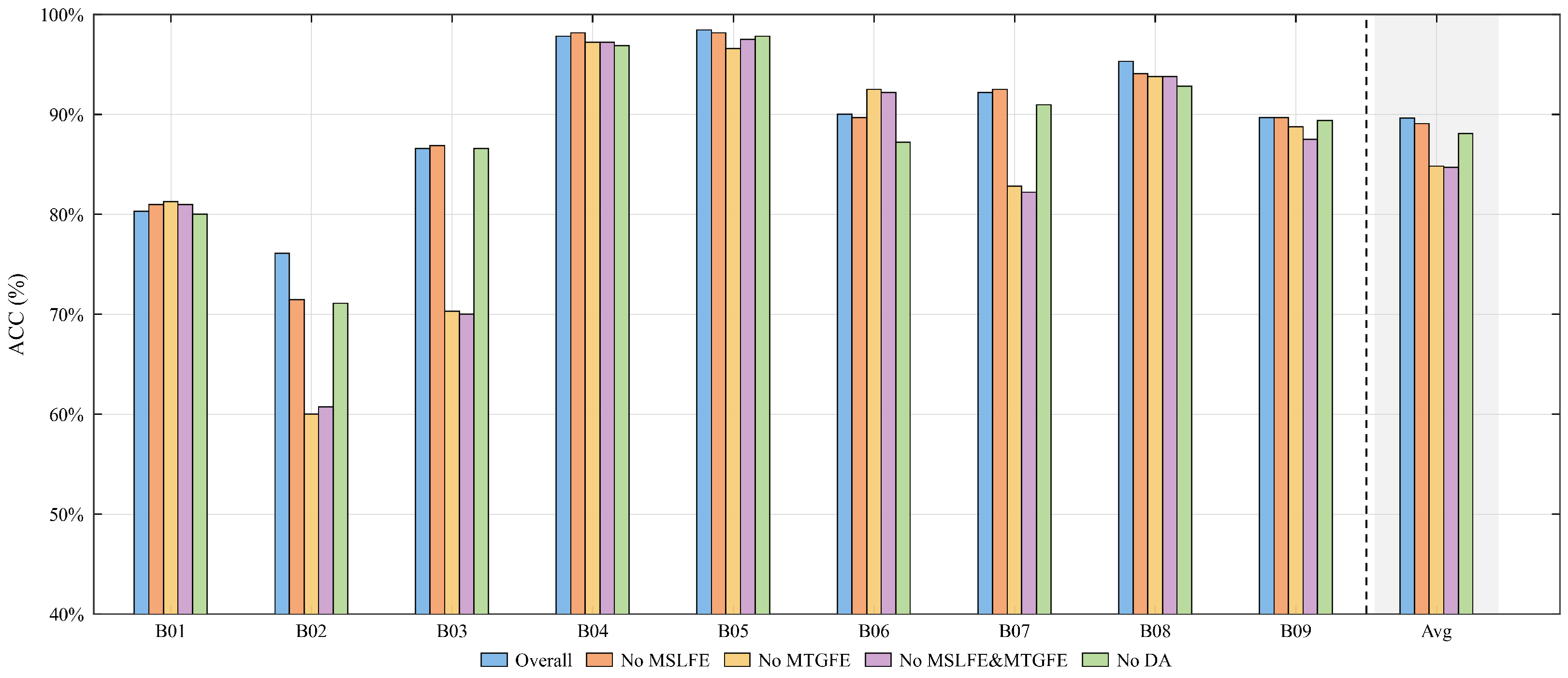
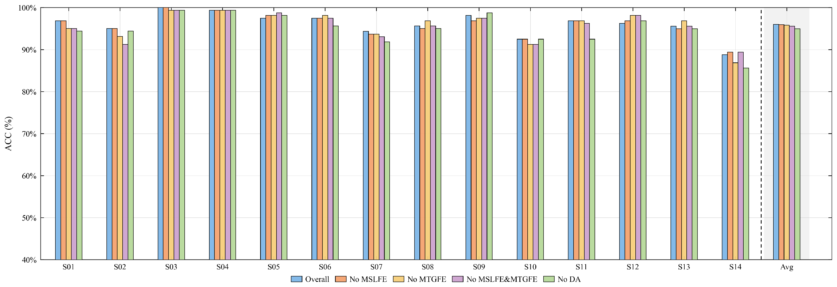
Figure 7, Figure 8 and Figure 9 show the classification accuracy for each subject across the BCI-IV-2a, BCI-IV-2b, and HGD datasets. It can be observed that removing the MSLFE or MTGFE modules leads to a notable performance drops. The MSLFE module contributes by capturing multi-scale spatial features from EEG signals, which allows the model to effectively extract fine-grained spatial patterns that are crucial for distinguishing motor imagery tasks. The MTGFE module, on the other hand, models global temporal dependencies across multiple channels, enabling the network to capture long-range interactions and temporal dynamics that are specific to each subject. Removing both modules results in the largest decrease in accuracy, highlighting the complementary nature of these modules. Their combined effect is essential for robust feature representation and improved generalization, demonstrating the unique advantage of integrating multi-scale spatial and global temporal modeling within HMT-Net.

The impact of data augmentation (DA) is also evident. Here, we adopt a segment and reconstruction strategy, which generates additional training samples by segmenting EEG trials and reconstructing them in novel combinations. Excluding DA consistently reduces performance across all datasets, demonstrating that augmenting the training data mitigates overfitting and enhances robustness. Overall, these results confirm that the MSLFE module, the MTGFE module, the hybrid Mamba–transformer design, and DA are all crucial for achieving strong and stable performance.

5.4. Parameters Analysis

5.4.1. Kernel Size

We first investigate the effect of different convolutional kernel combinations in the MSLFE module. As shown in

Table 11. Effect of different MSLFE kernel sizes on three datasets.

Kernel Size	Accuracy (%)
	BCI-IV 2a	BCI-IV 2b	HGD
{1, 3}	84.07	88.68	95.75
{3, 5}	83.14	88.82	95.84
{5, 7}	83.64	89.60	96.02

, the kernel combination $\{1,3\}$ achieves the best performance on BCI-IV-2a, while $\{5,7\}$ performs best on BCI-IV-2b and HGD. This difference may be related to the spatial resolution and signal characteristics of different datasets. For BCI-IV-2a, which contains 22 EEG channels, smaller kernels are sufficient to capture local discriminative patterns while avoiding excessive smoothing. In contrast, BCI-IV-2b contains only three bipolar channels and provides limited spatial information, while HGD uses high-density EEG recordings. In these cases, larger kernels can provide a wider receptive field, enabling the model to aggregate broader contextual information and capture more stable patterns. Therefore, the optimal kernel size depends on the spatial configuration and complexity of the dataset. The multi-scale design of MSLFE allows the network to balance fine-grained local feature extraction and broader contextual modeling for diverse EEG spatial patterns.

5.4.2. Heads

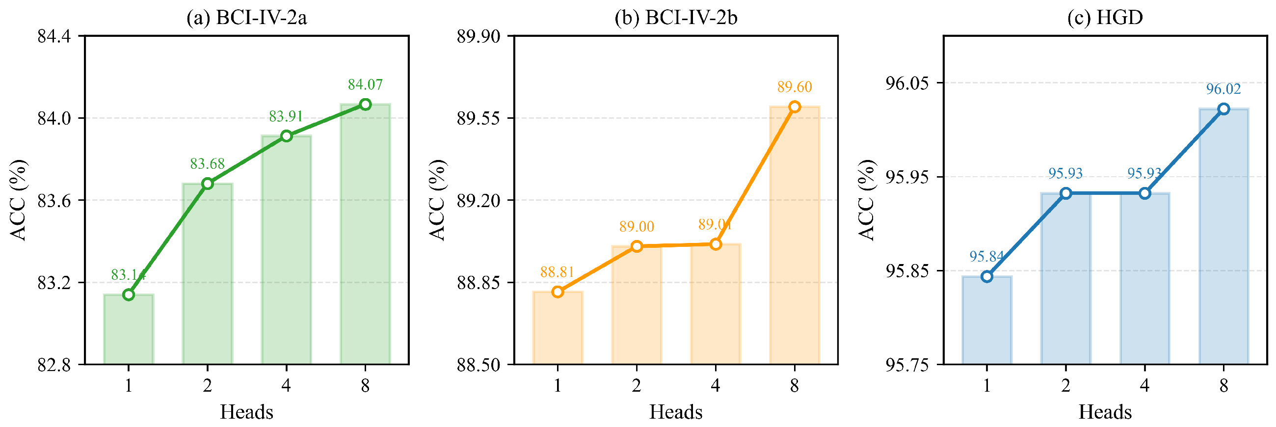
Figure 10 illustrates the influence of the number of attention heads in the MTGFE module. We evaluate 1, 2, 4, and 8 heads for each dataset. It can be observed that increasing the number of heads generally improves accuracy for all datasets, with 8 heads already providing a optimal performance. This suggests that 8 heads achieve a good balance between representation capability and computational efficiency.

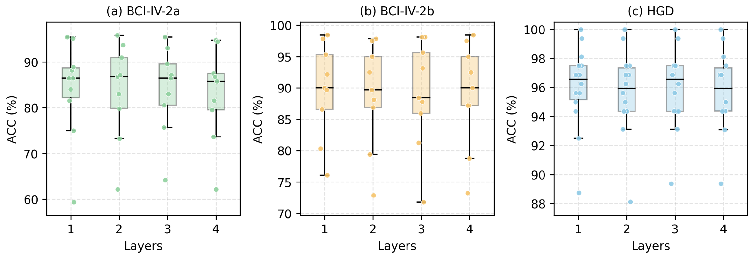
5.4.3. Layers

The effect of stacking multiple layers in the MTGFE module is shown in Figure 11. We test 1, 2, 3, and 4 layers for each dataset. Accuracy generally improves with more layers, reflecting the benefit of deeper feature extraction. However, adding too many layers does not significantly boost performance, and may increase computational cost. Hence, one layer was chosen as a suitable compromise for all three datasets.

5.5. Computational Complexity Analysis

To further evaluate the computational efficiency of the proposed HMT-Net, we compare it with representative baseline models on the BCI-IV-2a dataset in terms of trainable parameters, FLOPs, GPU memory consumption, inference time, and classification accuracy. The results are summarized in

Table 12. Computational complexity comparison on the BCI-IV-2a dataset.

Method	Params (M)	FLOPs (M/trial)	Memory (MB)	Time (ms/trial)	ACC (%)
ShallowConvNet [12]	0.0461	0.1684	11.8296	0.2263	67.94
DeepConvNet [12]	0.2829	13.7390	10.2837	0.4720	66.78
EEGNet [11]	0.0034	12.1951	10.8442	0.2840	72.42
FBCNet [24]	0.0118	1.1520	12.5122	1.3093	79.05
EEGConformer [14]	0.7896	63.8607	19.4385	2.4049	78.94
ATCNet [15]	0.1137	27.0113	15.7939	4.6530	77.47
TMSA-Net [17]	0.0077	13.3942	16.5127	0.7632	79.86
HMT-Net (Ours)	0.0648	57.2655	20.2539	3.0482	84.07

Note: FLOPs, GPU memory consumption, and inference time are measured using a single EEG trial with an input size of $22\times 1000$ and a batch size of 1. All measurements are conducted under the same environment with PyTorch 2.5.1 on an NVIDIA RTX 4090 GPU. Since the official implementation of FA-STTM is not publicly available, it is not included in this computational complexity comparison.

. It can be observed that HMT-Net contains only 0.0648M trainable parameters, which is much smaller than EEGConformer and ATCNet, indicating that the proposed model maintains a compact parameter scale. Although HMT-Net introduces relatively high FLOPs due to the hybrid Mamba–transformer modeling mechanism, its GPU memory consumption remains moderate. The inference time of HMT-Net is higher than that of lightweight CNN-based models, reflecting the additional computational cost required for global temporal dependency modeling. Nevertheless, HMT-Net achieves the highest classification accuracy among all compared methods. Overall, these results indicate that HMT-Net improves decoding accuracy at the cost of increased computation and inference time, while keeping the parameter count and memory consumption within a moderate range.

5.6. Visualization

To further analyze the representation capability and interpretability of the proposed model, we employ three complementary visualization methods. Specifically, t-distributed stochastic neighbor embedding (t-SNE) [39] is used to examine the distribution of learned feature embeddings, Gradient-weighted Class Activation Mapping (Grad-CAM) [40] is adopted to visualize task-relevant spatial activation patterns, and attention maps derived from the multi-head attention weights are further used to analyze temporal dependency modeling within the MTGFE module.

5.6.1. t-SNE

t-SNE is a nonlinear dimensionality reduction technique that maps high-dimensional features into a low-dimensional space while preserving local neighborhood structures, enabling intuitive visualization of clustering patterns among different classes.

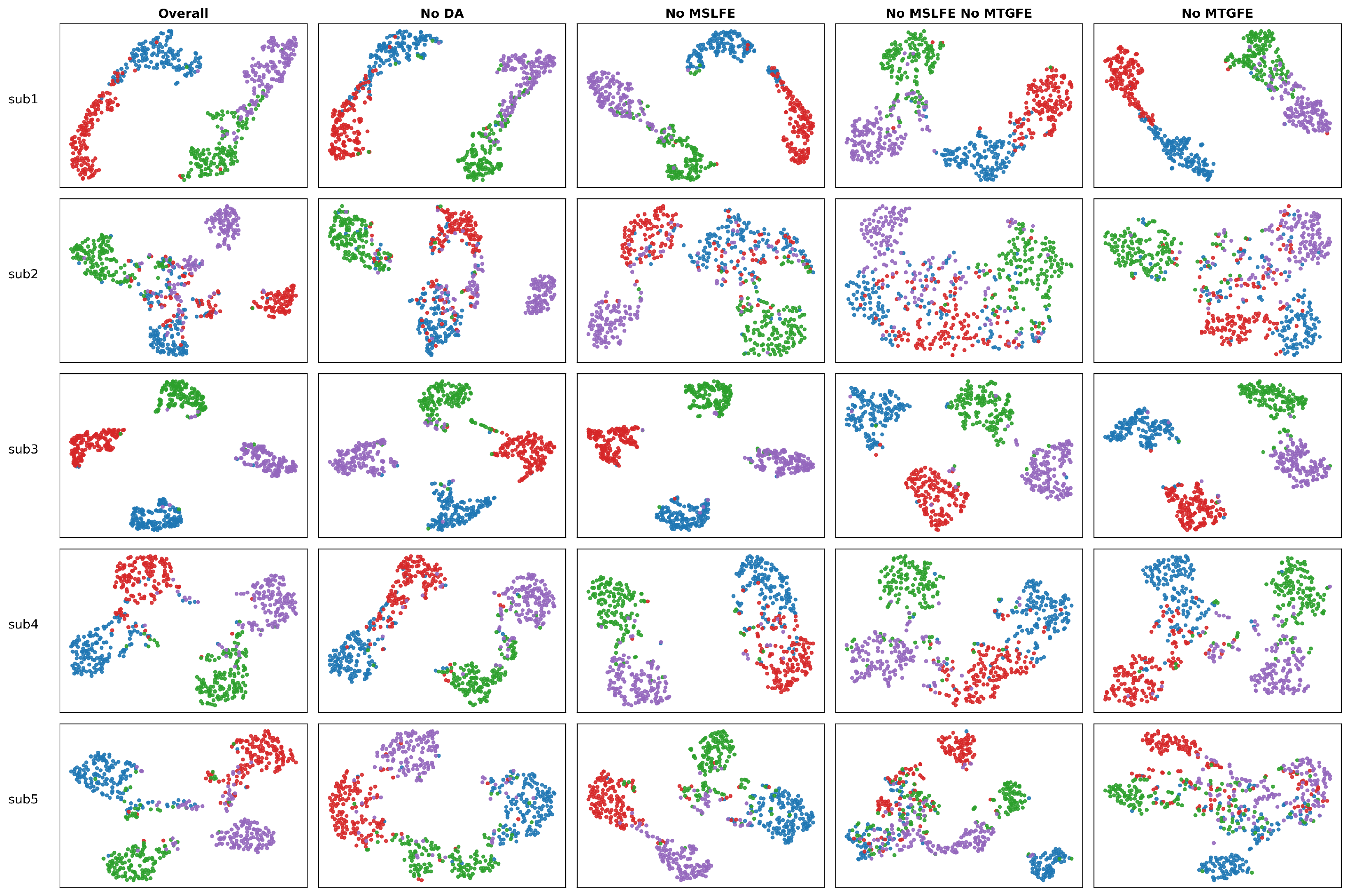
As shown in Figure 12, we present the t-SNE projections of the learned features for several representative subjects under different configurations, including the full model and its ablated variants. It is worth noting that the visualization is conducted on feature representations before the classifier, thus reflecting the quality of learned embeddings rather than the final classification outputs. The full model exhibits compact intra-class distributions and clear inter-class separation, indicating strong discriminative capability.

In contrast, removing data augmentation (No DA) leads to less compact clusters, suggesting reduced robustness. When the MSLFE module is removed (No MSLFE), class boundaries become less distinct, suggesting that multi-scale local feature extraction is important for capturing discriminative temporal patterns. Furthermore, removing both MSLFE and MTGFE (No MSLFE No MTGFE) results in significantly mixed distributions, demonstrating that the joint modeling of local and global features is essential. When the MTGFE module is excluded (No MTGFE), the clusters become more scattered, highlighting the importance of global dependency modeling.

Overall, these observations indicate that each component contributes to improving representation quality, and the complete model achieves the most compact and well-separated feature distributions.

5.6.2. Grad-CAM

To further investigate the interpretability of the proposed model, we employ Grad-CAM to illustrate the spatial activation patterns on EEG topographical maps.

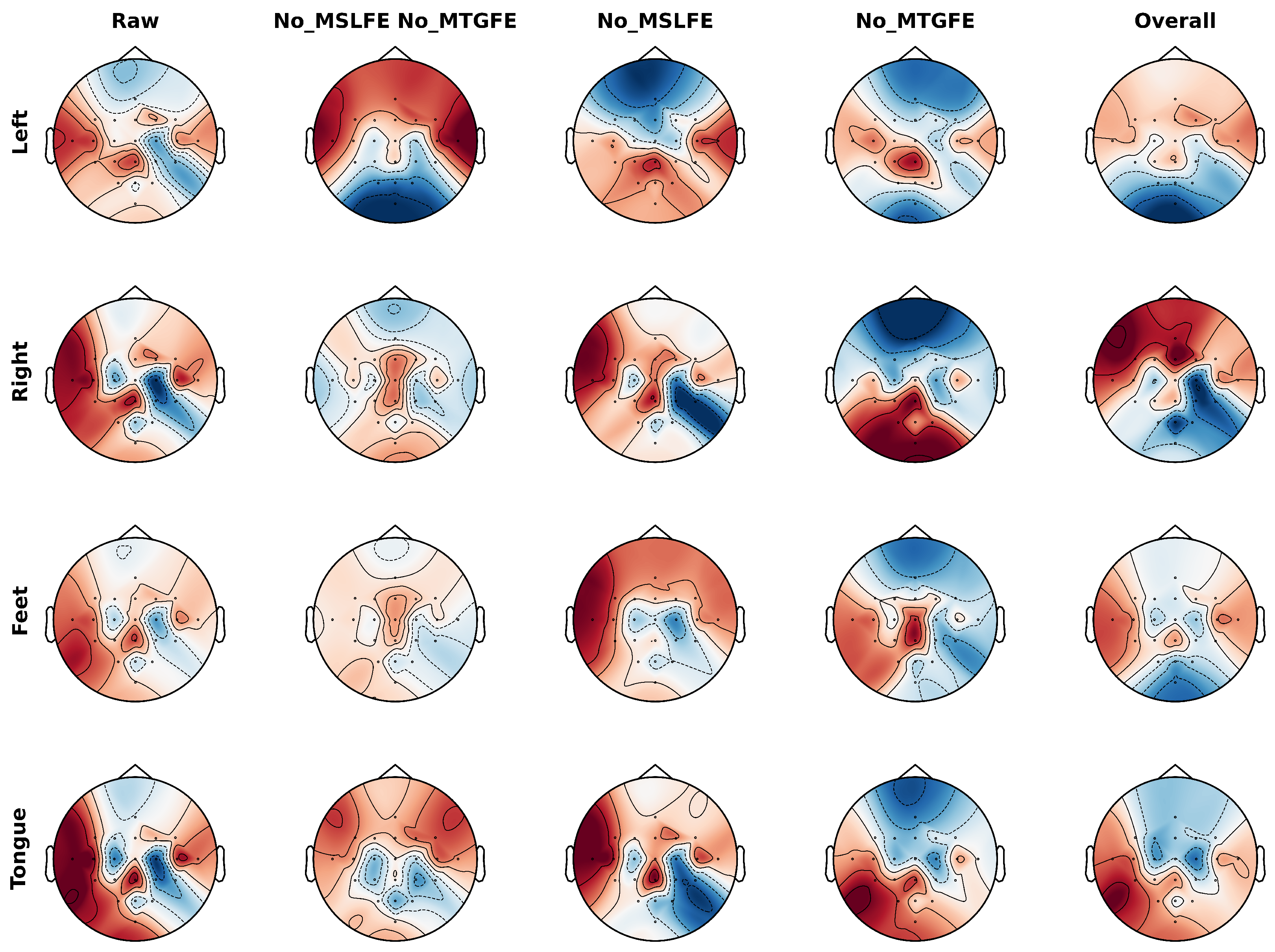
Grad-CAM highlights the regions in the input that contribute most to the model’s predictions, enabling an intuitive understanding of the learned representations. As shown in Figure 13, we present the activation maps for four motor imagery classes (Left, Right, Feet, and Tongue) under different model configurations.

The full model (Overall) produces focused and well-localized activation patterns, with prominent responses over task-relevant brain regions. For left and right hand imagery, stronger activations are observed in the contralateral motor cortex, which is consistent with established neurophysiological findings. Similarly, for feet and tongue tasks, the activations are concentrated in their corresponding motor areas, indicating that the model effectively captures meaningful spatial features.

In contrast, removing key components leads to degraded activation patterns. When both MSLFE and MTGFE are removed (No MSLFE No MTGFE), the activation maps become diffuse and less structured, suggesting a loss of spatial discriminability. Removing MSLFE alone (No MSLFE) results in less consistent activation regions, indicating weakened local feature extraction. When the MTGFE module is excluded (No MTGFE), the activations become more scattered and less focused, highlighting the importance of global dependency modeling in maintaining coherent spatial representations.

Overall, these results demonstrate that the proposed model can effectively identify task-relevant brain regions, and that each component contributes to learning meaningful and interpretable spatial patterns.

5.6.3. Attention Maps

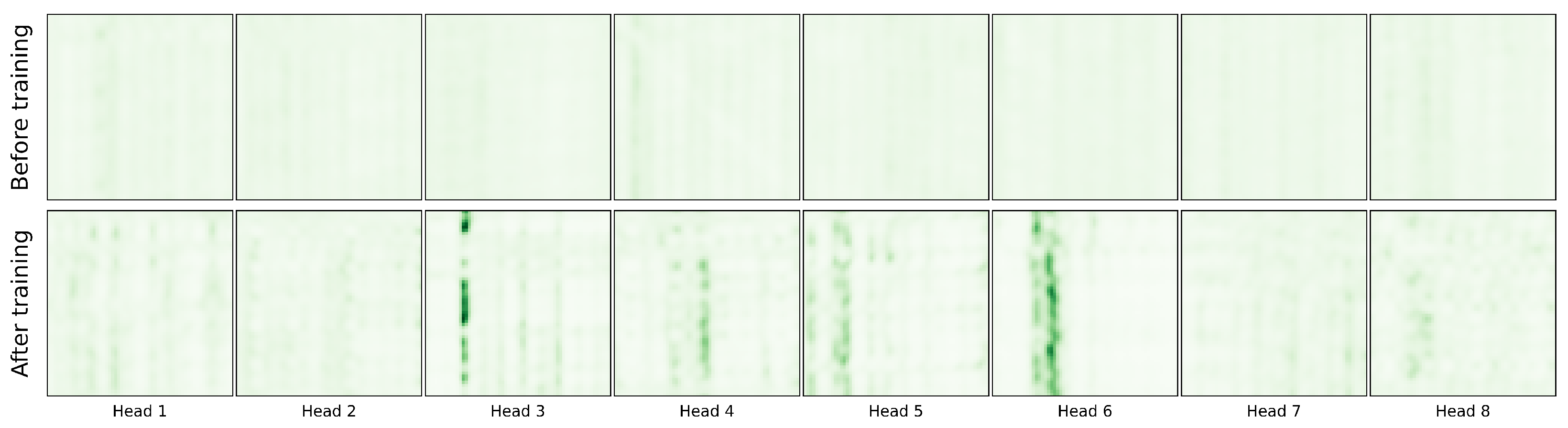
To complement the feature-level and spatial analyses, we illustrate the attention weight matrices from the MHA module in the MTGFE to investigate how the network models temporal dependencies within EEG sequences. In the MTGFE, the MHA component operates on features refined by the preceding Mamba module, capturing long-range interactions across temporal positions. Therefore, the attention maps offer a direct view of how the model distributes focus across the sequence to enhance temporal representation.

Figure 14 shows the attention maps of all eight heads for a representative subject, both before and after training. Prior to training, the attention distributions are relatively uniform and uninformative, reflecting the uninitialized state of the network. Following training, distinct patterns emerge, with certain heads emphasizing specific temporal regions while others capture broader interactions. This demonstrates that the multi-head design enables the network to model complementary temporal dependencies rather than relying on a single attention pattern.

These attention visualizations demonstrate that the MHA component in MTGFE captures structured temporal dependencies after training. Compared with the untrained network, trained attention patterns are more concentrated and head-specific, indicating that different heads capture complementary temporal relationships. Combined with the preceding t-SNE and Grad-CAM analyses, these results confirm that HMT-Net learns discriminative and interpretable representations across both spatial and temporal domains.

6. Discussion

Our proposed HMT-Net integrates multi-scale local feature extraction and hybrid temporal dependency modeling for MI-EEG decoding. The MSLFE module captures local temporal patterns at different receptive fields, while the MTGFE module combines Mamba-based sequence modeling with MHA-based global interaction modeling. The ablation results (Figure 7, Figure 8 and Figure 9) show that removing the MSLFE or MTGFE degrades performance, confirming their complementary roles in learning discriminative EEG representations. In addition, the MTGFE ablation results in Table 10 show that the Mamba–transformer variant achieves the best overall performance, indicating that Mamba and MHA provide complementary rather than redundant modeling capabilities.

The LOSO evaluation further demonstrates the cross-subject generalization capability of HMT-Net. As shown in Table 7, Table 8 and Table 9, HMT-Net achieves competitive or superior performance compared with ATCNet, EEGConformer, TMSA-Net, and FA-STTM. The improvement is particularly evident on the HGD dataset, where more subjects and high-density EEG channels provide richer spatial-temporal information. However, the gains on BCI-IV-2a and BCI-IV-2b are relatively moderate, and some comparisons do not reach statistical significance, indicating that cross-subject MI-EEG decoding remains challenging when training subjects are limited or inter-subject variability is strong.

Despite its effectiveness, HMT-Net still has several limitations. First, the integration of Mamba and MHA introduces additional computational cost. As shown in Table 12, HMT-Net maintains a compact number of trainable parameters and moderate memory consumption, but its FLOPs and inference time exceed those of lightweight CNNs. This indicates a trade-off between accuracy and computation, which is acceptable for offline MI-EEG analysis but real-time BCI applications may require further optimization. Second, individual differences remain an important factor affecting decoding performance. EEG signals vary across subjects due to neurophysiological patterns, electrode impedance, mental state, and task execution strategies. Although HMT-Net improves average performance, subject-wise variability persists, suggesting that a single shared model may not fully capture subject-specific characteristics. Future work may explore subject adaptation, domain generalization, or calibration-efficient learning. Third, practical deployment may face additional challenges, including EEG non-stationarity, artifacts, electrode displacement, and recording variations. These factors may reduce robustness under laboratory-trained models. Future studies should evaluate HMT-Net under diverse real-world scenarios and investigate more robust preprocessing, artifact handling, and adaptation strategies.

Overall, HMT-Net demonstrates strong potential for MI-EEG decoding by jointly modeling multi-scale local features and global temporal dependencies. The proposed architecture improves representation quality and classification performance, while the additional analyses reveal both its advantages and current limitations. Future work will focus on reducing computational cost, improving subject adaptation, and enhancing robustness in real-world BCI applications.

7. Conclusions

This study presents HMT-Net, a hierarchical model for MI-EEG decoding, systematically integrating multi-scale spatial and temporal feature extraction. The model combines the MSLFE module for capturing fine-grained spatial patterns across EEG channels with the MTGFE module for modeling long-range temporal dependencies. This design enables robust inter-subject generalization while effectively leveraging complementary information from both spatial and temporal domains. Extensive evaluations on BCI-IV-2a, BCI-IV-2b, and HGD demonstrate that HMT-Net achieves competitive or superior performance compared with representative state-of-the-art baselines. Ablation studies confirm the effectiveness of MSLFE and MTGFE, and the MTGFE-specific analysis further shows that Mamba and MHA provide complementary modeling capabilities. Moreover, targeted data augmentation via the segment reconstruction strategy consistently enhances robustness across subjects and datasets. Statistical significance tests further validate the reliability of the improvements, particularly on the HGD dataset. In addition, computational complexity analysis shows that HMT-Net maintains a compact parameter size and moderate memory consumption, although its FLOPs and inference time are higher than those of lightweight CNN-based models. Visualization results based on t-SNE, Grad-CAM, and attention maps further indicate that HMT-Net learns discriminative and interpretable representations from both spatial and temporal perspectives. Overall, HMT-Net achieves strong and stable decoding performance across multiple datasets and subjects, providing an effective framework for MI-EEG classification and a foundation for practical BCI applications.

References

1. Rashid, M.; Sulaiman, N.; Abdul Majeed, A.P.P.; Musa, R.M.; Ahmad, A.F.A.; Bari, B.S.; Khatun, S. Current status, challenges, and possible solutions of EEG-based brain-computer interface: A comprehensive review. Front. Neurorobot. 2020, 14, 25. [Google Scholar] [PubMed]
2. Altaheri, H.; Muhammad, G.; Alsulaiman, M.; Amin, S.U.; Altuwaijri, G.A.; Abdul, W.; Bencherif, M.A.; Faisal, M. Deep learning techniques for classification of electroencephalogram (EEG) motor imagery (MI) signals: A review. Neural Comput. Appl. 2023, 35, 14681–14722. [Google Scholar]
3. Hosseini, M.P.; Hosseini, A.; Ahi, K. A Review on Machine Learning for EEG Signal Processing in Bioengineering. IEEE Rev. Biomed. Eng. 2021, 14, 204–218. [Google Scholar] [CrossRef] [Scilit] [PubMed]
4. Roy, S.; Chowdhury, A.; McCreadie, K.; Prasad, G. Deep Learning Based Inter-subject Continuous Decoding of Motor Imagery for Practical Brain-Computer Interfaces. Front. Neurosci. 2020, 14, 918. [Google Scholar] [CrossRef] [Scilit] [PubMed]
5. Pfurtscheller, G.; Neuper, C. Motor Imagery and Direct Brain-Computer Communication. Proc. IEEE 2001, 89, 1123–1134. [Google Scholar] [CrossRef] [Scilit]
6. Cervera, M.A.; Soekadar, S.R.; Ushiba, J.; Millán, J.d.R.; Liu, M.; Birbaumer, N.; Garipelli, G. Brain-Computer Interfaces for Post-Stroke Motor Rehabilitation: A Meta-Analysis. Ann. Clin. Transl. Neurol. 2018, 5, 651–663. [Google Scholar] [CrossRef] [Scilit] [PubMed]
7. Singh, A.; Hussain, A.A.; Lal, S.; Guesgen, H.W. A Comprehensive Review on Critical Issues and Possible Solutions of Motor Imagery Based Electroencephalography Brain-Computer Interface. Sensors 2021, 21, 2173. [Google Scholar] [CrossRef] [Scilit] [PubMed]
8. Zhang, X.; Yao, L.; Wang, X.; Monaghan, J.J.M.; McAlpine, D.; Zhang, Y. A survey on deep learning-based non-invasive brain signals: Recent advances and new frontiers. J. Neural Eng. 2021, 18, 031002. [Google Scholar]
9. Saha, S.; Mamun, K.A.; Ahmed, K.; Mostafa, R.; Naik, G.R.; Darvishi, S.; Khandoker, A.H.; Baumert, M. Progress in Brain Computer Interface: Challenges and Opportunities. Front. Syst. Neurosci. 2021, 15, 578875. [Google Scholar] [CrossRef] [Scilit] [PubMed]
10. Tibrewal, N.; Leeuwis, N.; Alimardani, M. Classification of Motor Imagery EEG Using Deep Learning Increases Performance in Inefficient BCI Users. PLoS ONE 2022, 17, e0268880. [Google Scholar] [CrossRef] [Scilit] [PubMed]
11. Lawhern, V.J.; Solon, A.J.; Waytowich, N.R.; Gordon, S.M.; Hung, C.P.; Lance, B.J. EEGNet: A compact convolutional neural network for EEG-based brain-computer interfaces. J. Neural Eng. 2018, 15, 056013. [Google Scholar] [PubMed]
12. Schirrmeister, R.T.; Springenberg, J.T.; Fiederer, L.D.J.; Glasstetter, M.; Eggensperger, K.; Tangermann, M.; Hutter, F.; Burgard, W.; Ball, T. Deep learning with convolutional neural networks for EEG decoding and visualization. Hum. Brain Mapp. 2017, 38, 5391–5420. [Google Scholar] [CrossRef] [Scilit] [PubMed]
13. Roots, K.; Muhammad, Y.; Muhammad, N. Fusion convolutional neural network for cross-subject EEG motor imagery classification. Computers 2020, 9, 72. [Google Scholar] [CrossRef] [Scilit]
14. Song, Y.; Zheng, Q.; Liu, B.; Gao, X. EEG Conformer: Convolutional Transformer for EEG decoding and visualization. IEEE Trans. Neural Syst. Rehabil. Eng. 2023, 31, 710–719. [Google Scholar] [PubMed]
15. Altaheri, H.; Muhammad, G.; Alsulaiman, M. Physics-informed attention temporal convolutional network for EEG-based motor imagery classification. IEEE Trans. Ind. Inform. 2023, 19, 2249–2258. [Google Scholar] [CrossRef] [Scilit]
16. Zhang, J.; Li, K.; Yang, B.; Han, X. Local and Global Convolutional Transformer-Based Motor Imagery EEG Classification. Front. Neurosci. 2023, 17, 1219988. [Google Scholar] [CrossRef] [Scilit] [PubMed]
17. Zhao, Q.; Zhu, W. TMSA-Net: A Novel Attention Mechanism for Improved Motor Imagery EEG Signal Processing. Biomed. Signal Process. Control 2025, 102, 107189. [Google Scholar] [CrossRef] [Scilit]
18. Gu, A.; Dao, T. Mamba: Linear-time sequence modeling with selective state spaces. arXiv 2023, arXiv:2312.00752. [Google Scholar]
19. Gu, A.; Goel, K.; Ré, C. Efficiently Modeling Long Sequences with Structured State Spaces. In Proceedings of the International Conference on Learning Representations, Virtual, 25–29 April 2022. [Google Scholar]
20. Pfurtscheller, G.; Lopes da Silva, F.H. Event-Related EEG/MEG Synchronization and Desynchronization: Basic Principles. Clin. Neurophysiol. 1999, 110, 1842–1857. [Google Scholar] [CrossRef] [Scilit] [PubMed]
21. Pfurtscheller, G.; Brunner, C.; Schlögl, A.; Lopes da Silva, F.H. Mu Rhythm (De)Synchronization and EEG Single-Trial Classification of Different Motor Imagery Tasks. NeuroImage 2006, 31, 153–159. [Google Scholar] [CrossRef] [Scilit] [PubMed]
22. Chen, X.; Teng, X.; Chen, H.; Pan, Y.; Geyer, P. Toward Reliable Signals Decoding for Electroencephalogram: A Benchmark Study to EEGNeX. Biomed. Signal Process. Control 2024, 87, 105475. [Google Scholar] [CrossRef] [Scilit]
23. Hamedi, M.; Salleh, S.H.; Noor, A.M. Electroencephalographic Motor Imagery Brain Connectivity Analysis for BCI: A Review. Neural Comput. 2016, 28, 999–1041. [Google Scholar] [CrossRef] [Scilit] [PubMed]
24. Mane, R.; Chew, E.; Chua, K.; Ang, K.K.; Robinson, N.; Vinod, A.P.; Lee, S.W.; Guan, C. FBCNet: A multi-view convolutional neural network for Brain-Computer Interface. arXiv 2021, arXiv:2104.01233. [Google Scholar]
25. Li, Y.; Guo, L.; Liu, Y.; Liu, J.; Meng, F. A Temporal-Spectral-Based Squeeze-and-Excitation Feature Fusion Network for Motor Imagery EEG Decoding. IEEE Trans. Neural Syst. Rehabil. Eng. 2021, 29, 1534–1545. [Google Scholar] [CrossRef] [Scilit] [PubMed]
26. Guo, M.; Han, X.; Liu, H.; Zhu, J.; Zhang, J.; Bai, Y.; Ni, G. MI-Mamba: A Hybrid Motor Imagery Electroencephalograph Classification Model with Mamba’s Global Scanning. Ann. N. Y. Acad. Sci. 2025, 1544, 242–253. [Google Scholar] [CrossRef] [Scilit] [PubMed]
27. Gui, Y.; Chen, M.; Su, Y.; Luo, G.; Yang, Y. EEGMamba: Bidirectional State Space Model with Mixture of Experts for EEG Multi-Task Classification. arXiv 2024, arXiv:2407.20254. [Google Scholar]
28. Vaswani, A.; Shazeer, N.; Parmar, N.; Uszkoreit, J.; Jones, L.; Gomez, A.N.; Kaiser, L.; Polosukhin, I. Attention is all you need. Adv. Neural Inf. Process. Syst. 2017, arXiv:1706.03762. [Google Scholar]
29. Tangermann, M.; Müller, K.R.; Aertsen, A.; Birbaumer, N.; Braun, C.; Brunner, C.; Leeb, R.; Mehring, C.; Miller, K.J.; Müller-Putz, G.R.; et al. Review of the BCI competition IV. Front. Neurosci. 2012, 6, 55. [Google Scholar] [CrossRef] [Scilit] [PubMed]
30. Lotte, F. Signal processing approaches to minimize or suppress calibration time in oscillatory activity-based brain–computer interfaces. Proc. IEEE Inst. Electr. Electron. Eng. 2015, 103, 871–890. [Google Scholar]
31. Zhao, W.; Jiang, X.; Zhang, B.; Xiao, S.; Weng, S. CTNet: A convolutional transformer network for EEG-based motor imagery classification. Sci. Rep. 2024, 14, 20237. [Google Scholar] [CrossRef] [Scilit] [PubMed]
32. Gao, M.; Gao, C.; Yao, Z.; Zhu, W. FA-STTM: A hybrid Transformer-Mamba network for motor imagery EEG classification. Neurocomputing 2026, 669, 132481. [Google Scholar]
33. Ang, K.K.; Chin, Z.Y.; Zhang, H.; Guan, C. Filter bank common spatial pattern (FBCSP) in brain-computer interface. In 2008 IEEE International Joint Conference on Neural Networks (IEEE World Congress on Computational Intelligence); IEEE: Piscataway, NJ, USA, 2008. [Google Scholar]
34. Bai, S.; Kolter, J.Z.; Koltun, V. An empirical evaluation of generic convolutional and recurrent networks for sequence modeling. arXiv 2018, arXiv:1803.01271. [Google Scholar]
35. Liu, Z.; Wang, Y.; Vaidya, S.; Ruehle, F.; Halverson, J.; Soljačić, M.; Hou, T.Y.; Tegmark, M. KAN: Kolmogorov-Arnold Networks. arXiv 2024, arXiv:2404.19756. [Google Scholar]
36. Wimpff, M.; Gizzi, L.; Zerfowski, J.; Yang, B. EEG motor imagery decoding: A framework for comparative analysis with channel attention mechanisms. J. Neural Eng. 2024, 21, 036020. [Google Scholar] [CrossRef] [Scilit] [PubMed]
37. Powers, D.M.W. Evaluation: From precision, recall and F-measure to ROC, informedness, markedness and correlation. arXiv 2020, arXiv:2010.16061. [Google Scholar]
38. Cohen, J. A coefficient of agreement for nominal scales. Educ. Psychol. Meas. 1960, 20, 37–46. [Google Scholar] [CrossRef] [Scilit]
39. van der Maaten, L.; Hinton, G. Visualizing Data using t-SNE. J. Mach. Learn. Res. 2008, 9, 2579–2605. [Google Scholar]
40. Selvaraju, R.R.; Cogswell, M.; Das, A.; Vedantam, R.; Parikh, D.; Batra, D. Grad-CAM: Visual explanations from deep networks via gradient-based localization. In 2017 IEEE International Conference on Computer Vision (ICCV); IEEE: Piscataway, NJ, USA, 2017. [Google Scholar]
Figure 1. Overall architecture of the proposed HMT-Net. The model consists of a shallow feature embedding (SFE) module, a multi-scale local feature extractor (MSLFE) module, a Mamba–transformer global feature encoder (MTGFE) module, and a classifier.
Mathematics 14 02149 g001
Figure 2. Structure of the Mamba block, consisting of two state-space models (SSMs).
Mathematics 14 02149 g002
Figure 3. Structure of the multi-head attention (MHA) mechanism.
Mathematics 14 02149 g003
Figure 4. Radar chart comparison of different models on three datasets. The metrics include ACC, kappa, F1-score, recall, and precision.
Mathematics 14 02149 g004
Figure 5. Average normalized confusion matrices of HMT-Net on three MI-EEG datasets.
Mathematics 14 02149 g005
Figure 6. Accuracy of each subject on the BCI-IV-2a dataset under the LOSO setting.
Mathematics 14 02149 g006
Figure 7. Ablation study results on the BCI-IV-2a dataset.
Mathematics 14 02149 g007
Figure 8. Ablation study results on the BCI-IV-2b dataset.
Mathematics 14 02149 g008
Figure 9. Ablation study results on the HGD dataset.
Mathematics 14 02149 g009
Figure 10. Effect of different numbers of attention heads on three datasets.
Mathematics 14 02149 g010
Figure 11. Effect of different numbers of layers on three datasets.
Mathematics 14 02149 g011
Figure 12. t-SNE visualization of learned feature representations on the BCI-IV-2a dataset for five subjects. Each row corresponds to a different subject, and each column represents a different model configuration: the full model (Overall), without data augmentation (No DA), without MSLFE (No MSLFE), without both MSLFE and MTGFE (No MSLFE No MTGFE), and without MTGFE (No MTGFE).
Mathematics 14 02149 g012
Figure 13. Grad-CAM representation of EEG topographical activation maps on the BCI-IV-2a dataset for subject 3.
Mathematics 14 02149 g013
Figure 14. Attention maps of the MTGFE on the BCI-IV-2a dataset for a representative subject. The first row shows the attention before training, and the second row shows the attention after training. Each column corresponds to one of the eight attention heads.
Mathematics 14 02149 g014