Localized Hermite Method of Approximate Particular Solutions for Solving the Helmholtz Equation

Abstract

This paper proposes a localized Hermite method of approximate particular solutions (LHMAPS) for solving the 2D inhomogeneous Helmholtz-type equations. Building on the local scheme of the localized method of approximate particular solutions (LMAPS) for the Helmholtz-type differential operator, LHMAPS employs Hermite-type local approximations involving both the solution values and their Laplacian to improve the accuracy of LMAPS. The polyharmonic spline (PS) radial basis functions and polynomial basis functions are considered in the formulation of LHMAPS. Numerical experiments are presented to demonstrate the enhanced accuracy achieved by employing Hermite-type local approximations.

1. Introduction

Meshfree methods based on radial basis functions (RBFs) for numerical approximation and for solving differential equations constitute an important class of numerical methods in scientific computing [1,2,3,4,5,6]. These methods have been developed to address the limitations of traditional mesh-based methods in problems involving complex geometries, large deformations, moving boundaries, and high-dimensional domains, where mesh generation and remeshing can become difficult or computationally expensive. They have been applied in a variety of industrial and engineering settings, such as fluid dynamics, wave propagation, geophysical modeling, and materials science [7,8,9,10].

Compared with classical finite element or finite difference methods, meshfree methods offer the advantage of avoiding mesh generation and providing flexible node placement, which simplifies the handling of complex or evolving geometries. However, although global RBF-based methods can achieve high-order accuracy with relatively simple formulations, they also have several limitations, including high computational cost associated with global approximations, potential ill-conditioning of interpolation matrices, and sensitivity to shape parameter selection or stencil configuration in localized variants [1]. Many of these issues can be alleviated by adopting localized schemes [2,6,11]. Among various localized RBF collocation methods, the localized method of approximate particular solutions (LMAPS), which employs particular solutions of radial basis functions to locally approximate the solution of a differential equation, rather than using the RBFs themselves, has attracted considerable attention due to its high accuracy [11,12,13]. LMAPS using particular solutions of polynomial basis functions has also been investigated in [14,15,16].

The localized Hermite method of approximate particular solutions (LHMAPS) was proposed in [17,18] for solving the Poisson equation and convection–reaction–diffusion equations. This method resembles compact finite difference schemes [19,20] in its local approximation of the Laplace operator around each interior collocation point, providing a combined local approximation that incorporates both RBFs and their particular solutions. Several related RBF collocation methods using Hermite interpolation have also been developed, including the Hermite-type radial basis function-based differential quadrature method (H-RBF-DQ), the localized Hermitian (symmetric) meshless method using RBFs, and the compact RBF-FD (RBF-HFD) methods [21,22,23]. Numerical experiments demonstrate that LHMAPS significantly improves the accuracy and convergence rates of traditional LMAPS for multiquadric (MQ), Gaussian (GA), and polyharmonic spline (PS) radial basis functions at the cost of only a slight increase in computational effort. A comparison of the computational costs between LMAPS and LHMAPS using these radial basis functions can be found in Table 2 of [17].

However, existing studies on LHMAPS in [17,18] have considered only particular solutions of MQ, GA, and PS radial basis functions for the Laplace operator. In this paper, we investigate LHMAPS using PS radial basis functions and polynomial basis functions whose particular solutions for Helmholtz-type differential operators have been derived previously [11,24,25]. More specifically, in this paper, we consider LMHAPS using these two types of particular solutions for solving the inhomogeneous Helmholtz equation with the Dirichlet boundary condition:

$$\begin{array}{c}\hfill {\displaystyle \left\{\begin{array}{cc}\Delta u\pm {\lambda }^{2}u=f,\hfill & \mathrm{i}\mathrm{n}\mathrm{\Omega },\hfill \\ u=g,\hfill & \mathrm{o}\mathrm{n}\mathsf{\partial }\mathrm{\Omega }.\hfill \end{array}\right.}\end{array}$$

(1)

where $\lambda$ is a nonzero real constant, and $\mathrm{\Omega }\subset {\mathbb{R}}^2$ is a bounded, simply connected domain with a piecewise smooth boundary $\mathsf{\partial }\mathrm{\Omega }$. f and g are real-valued functions defined on $\mathrm{\Omega }$ and $\mathsf{\partial }\mathrm{\Omega }$, respectively.

The remainder of this article is organized as follows. A brief introduction of LMAPS with polynomial basis functions and PS radial basis functions is given in Section 2.4. The LHMAPS schemes using polynomial basis functions and PS radial basis functions are presented in Section 3 and Section 4, respectively. Numerical experiments are discussed in Section 5, and the main findings are summarized in Section 6.

2. A Review of LMAPS

In this section, we first introduce polynomial basis functions, PS radial basis functions, and their particular solutions under the Helmholtz-type differential operator ${\mathcal{L}}_{\pm }:=\Delta \pm {\lambda }^2$. For simplicity, we use $\mathcal{L}$ to denote ${\mathcal{L}}_{\pm }$ when presenting the numerical schemes for LMAPS and LHMAPS.

Then, we elaborate on the notations used for the collocation points and local neighborhoods. Following this, a brief review of LMAPS using PS and polynomial basis functions is presented.

2.1. Polynomial Basis Functions and PS Radial Basis Functions

The polynomial basis functions of degree k used in LMAPS are usually denoted by $\psi \left(\mathit{x}\right)=x_1^{\xi }{x}_2^{\eta }$ with non-negative integers $\xi$ and $\eta$ satisfying $0\le \xi ,\eta \le k$ and $\xi +\eta =k$ (see [14,15,16]).

A particular solution of $\psi \left(\mathit{x}\right)$ for the general second-order linear partial differential operator $\mathcal{D}$ with constant coefficients ${\left\{a_i\right\}}_{i=1}^6$ and $a_6\ne 0$, which is denoted by $\mathrm{\Psi }\left(\mathit{x}\right)$, satisfies

$$\mathcal{D}\mathrm{\Psi }\left(\mathit{x}\right):=\left(a_1{\displaystyle \frac{{\mathsf{\partial }}^2}{\mathsf{\partial }{x}_1^2}}+a_2{\displaystyle \frac{{\mathsf{\partial }}^2}{\mathsf{\partial }{x}_1\mathsf{\partial }{x}_2}}+a_3{\displaystyle \frac{{\mathsf{\partial }}^2}{\mathsf{\partial }{x}_2^2}}+a_4{\displaystyle \frac{\mathsf{\partial }}{\mathsf{\partial }{x}_1}}+a_5{\displaystyle \frac{\mathsf{\partial }}{\mathsf{\partial }{x}_2}}+a_6\right)\mathrm{\Psi }\left(\mathit{x}\right)=\psi \left(\mathit{x}\right).$$

It has been proven in [14] that $\mathrm{\Psi }\left(\mathit{x}\right)$ can be expressed as follows:

$$\mathrm{\Psi }\left(\mathit{x}\right)={\displaystyle \frac{1}{a_6}}{\displaystyle \sum _{j=0}^k}{\left({\displaystyle \frac{-1}{a_6}}\right)}^j{\mathcal{D}}^j\left(x_1^{\xi }{x}_2^{\eta }\right).$$

(2)

In particular, a specific solution of the polynomial basis function $\psi \left(\mathit{x}\right)$ for the differential operator ${\mathcal{L}}_{+}$ has the following expression [25]:

$$\mathrm{\Psi }\left(\mathit{x}\right)={\displaystyle \sum _{i=0}^{[\eta /2]}}{\displaystyle \sum _{j=0}^{[\eta /2]}}{\displaystyle \frac{{(-1)}^{i+j}(i+j)!\xi !\eta !x_1^{\xi -2i}{x}_2^{\eta -2j}}{{\lambda }^{2i+2j+2}i!j!(\xi -2i)!(\eta -2j)!}}.$$

In numerical experiments, we use (2) to compute the particular solution for both differential operators ${\mathcal{L}}_{\pm }$, which is used in the localized numerical schemes of LMAPS and LHMAPS.

For the PS radial basis function $\varphi \left(r\right):=r^{2\omega }\ln (r)$ of positive integer order $\omega$, let $\mathrm{\Phi }\left(r\right)$ denote a particular solution of ${\mathcal{L}}_{-}\mathrm{\Phi }\left(r\right)=\varphi \left(r\right)$, where r stands for the Euclidean norm $\parallel \mathit{x}\parallel$ for any $\mathit{x}\in {\mathbb{R}}^2$. The particular solutions associated with PS radial basis functions of orders $\omega =1,2,3$ for the differential operator ${\mathcal{L}}_{-}$ were obtained in [11,24]. The corresponding PS radial basis functions are listed in

Table 1. PS radial basis functions and their particular solutions for ${\mathcal{L}}_{-}$.

$\mathit{\varphi }\left(\mathit{r}\right)$	$\mathrm{\Phi }\left(\mathit{r}\right)$
PS1 = $r^2\ln (r)$	$\left\{\begin{array}{c}\hspace{1em}-{\displaystyle \frac{4}{{\lambda }^4}}(K_0\left(\lambda r\right)+\ln (r))-{\displaystyle \frac{r^2\ln (r)}{{\lambda }^2}}-{\displaystyle \frac{4}{{\lambda }^4}},\mathrm{if}r>0,\hfill \\ \hspace{1em}{\displaystyle \frac{4}{{\lambda }^4}}(\gamma +\ln ({\displaystyle \frac{\lambda }{2}}))-{\displaystyle \frac{4}{{\lambda }^4}},\mathrm{if}r=0.\hfill \end{array}\right.$
PS2 = $r^4\ln \left(r\right)$	$\left\{\begin{array}{c}\hspace{1em}-{\displaystyle \frac{64}{{\lambda }^6}}(K_0\left(\lambda r\right)+\ln (r))-{\displaystyle \frac{r^2\ln (r)}{{\lambda }^2}}({\displaystyle \frac{16}{{\lambda }^2}}+r^2)-{\displaystyle \frac{8r^2}{{\lambda }^4}}-{\displaystyle \frac{96}{{\lambda }^6}},\mathrm{if}r>0,\hfill \\ \hspace{1em}{\displaystyle \frac{64}{{\lambda }^6}}(\gamma +\ln ({\displaystyle \frac{\lambda }{2}}))-{\displaystyle \frac{96}{{\lambda }^6}},\mathrm{if}r=0.\hfill \end{array}\right.$
PS3 = $r^6\ln \left(r\right)$	$\left\{\begin{array}{c}\hspace{1em}-{\displaystyle \frac{2304}{{\lambda }^8}}(K_0\left(\lambda r\right)+\ln \left(r\right))-{\displaystyle \frac{r^2\ln \left(r\right)}{{\lambda }^2}}({\displaystyle \frac{576}{{\lambda }^4}}+{\displaystyle \frac{36r^2}{{\lambda }^2}}+r^4),\mathrm{if}r>0,\hfill \\ \hspace{1em}-{\displaystyle \frac{12r^2}{{\lambda }^4}}({\displaystyle \frac{40}{{\lambda }^2}}+r^2)-{\displaystyle \frac{4224}{{\lambda }^8}},\mathrm{if}r=0.\hfill \end{array}\right.$

and are denoted by PS1, PS2, and PS3, respectively.

2.2. Notations for the Collocation Points and Local Neighbourhoods

Let $\mathit{x}=(x,y)$ be a generic point in ${\mathbb{R}}^2$. Let $\mathit{X}:={\mathit{X}}^I\cup {\mathit{X}}^B$ be the the set of collocation points in $\overline{\mathrm{\Omega }}$, where ${\mathit{X}}^I:={\left\{{\mathit{x}}_j\right\}}_1^{N_I}$ and ${\mathit{X}}^B={\left\{{\mathit{x}}_i^B\right\}}_1^{N_B}$ denote the set of interior points in $\mathrm{\Omega }$ and the set of boundary collocation points on $\mathsf{\partial }\mathrm{\Omega }$, respectively. For simplicity, we also let $\mathit{X}={\left\{{\mathit{x}}_j\right\}}_1^N$ with $N:=N_I+N_B$.

For an interior collocation point ${\mathit{x}}_s\in {\mathit{X}}^I$, a neighborhood ${\mathrm{\Omega }}_s$ is determined by a fixed number of nearest collocation points. We assume that ${\mathrm{\Omega }}_s$ contains n collocation points ${\mathit{X}}^{\left[s\right]}:={\left\{{\mathit{x}}_j^{\left[s\right]}\right\}}_{j=1}^n\subset \mathit{X}$, containing ${\mathit{x}}_s$ and its nearest $n-1$ neighbors. Without loss of generality, we set ${\mathit{x}}_1^{\left[s\right]}={\mathit{x}}_s$. Moreover, we choose ${\mathit{X}}_H^{\left[s\right]}\subseteq {\mathit{X}}^{\left[s\right]}$ for the Hermite interpolation. For instance, if $\mathit{X}$ contains structured 2D rectangular nodes, a popular nine-point stencil centered at ${\mathit{x}}_s$ contains ${\mathit{x}}_s$ and its nearest eight neighbors, four of which are also used for Hermite interpolation.

2.3. LMAPS Using PS Radial Basis Functions

For each ${\mathit{x}}_s\in {\mathit{X}}^I$, the LMAPS using PS radial basis functions seeks a local approximation $\tilde{u}$ to u in ${\mathrm{\Omega }}_s$ as follows:

$$\tilde{u}\left(\mathit{x}\right)={\displaystyle \sum _{j=1}^n}{\alpha }_j^{\left[s\right]}\mathrm{\Phi }(\parallel \mathit{x}-{\mathit{x}}_j^{\left[s\right]}\parallel )+{\displaystyle \sum _{j=1}^{𝓁}}{\gamma }_j^{\left[s\right]}{p}_j\left(\mathit{x}\right),$$

(3)

where ${\alpha }_j^{\left[s\right]}$ ($j=1,\cdots ,n$) and ${\gamma }_j^{\left[s\right]}$ ($j=1,\cdots ,𝓁$) are real constants, $p_j\left(\mathit{x}\right)$ denotes all monomials of degree no more than k with $𝓁=(k+1)(k+2)/2$. The initial LMAPS method proposed in [11] did not incorporate auxiliary polynomials $p_j\left(\mathit{x}\right)$. A more detailed exploration of the role of the auxiliary polynomials of degree k in enhancing the accuracy of LMAPS using PS radial basis functions was studied in [12]. For instance, if we set $k=1$, then $𝓁=3$ and ${\left\{p_j\left(\mathit{x}\right)\right\}}_{j=1}^3=\{1,x_1,x_2\}$.

Define coefficient vectors ${\mathit{\alpha }}^{\left[s\right]}:={({\alpha }_1^{\left[s\right]},\cdots ,{\alpha }_n^{\left[s\right]})}^T$ and ${\mathit{\gamma }}^{\left[s\right]}:={({\gamma }_1^{\left[s\right]},\cdots ,{\gamma }_{𝓁}^{\left[s\right]})}^T$. Here and throughout the paper, the superscript T denotes the transpose of a vector or matrix.

Next, we rewrite (3) as the following linear system by selecting $\mathit{x}\in {\mathit{X}}^{\left[s\right]}$

$${\mathit{U}}^{\left[s\right]}=\left(\begin{array}{cc}{\mathbf{\Phi }}_{nn}& {\mathit{P}}_{n𝓁}\end{array}\right)\left(\begin{array}{c}{\mathit{\alpha }}^{\left[s\right]}\\ {\mathit{\gamma }}^{\left[s\right]}\end{array}\right),$$

(4)

where

$$\begin{array}{cc}\hfill {\mathit{U}}^{\left[s\right]}& :={\left[u\left({\mathit{x}}_1^{\left[s\right]}\right),\cdots ,u\left({\mathit{x}}_n^{\left[s\right]}\right)\right]}_{n\times 1}^T,\hfill \\ \hfill {\mathbf{\Phi }}_{nn}& :={\left[\mathrm{\Phi }(\parallel {\mathit{x}}_i^{\left[s\right]}-{\mathit{x}}_j^{\left[s\right]}\parallel )\right]}_{n\times n},{\mathit{P}}_{n𝓁}:={\left[p_j\left({\mathit{x}}_i^{\left[s\right]}\right)\right]}_{n\times 𝓁}.\hfill \end{array}$$

In addition to (4), we impose ℓ auxiliary constraints

$${\displaystyle \sum _{j=1}^n}{\alpha }_j{p}_i\left({\mathit{x}}_j^{\left[s\right]}\right)=0,i=1,\cdots ,𝓁,$$

to yield a symmetric local weight matrix in the following linear system

$$\left(\begin{array}{c}{\mathit{U}}^{\left[s\right]}\\ 0\end{array}\right)=\left(\begin{array}{cc}{\mathbf{\Phi }}_{nn}& {\mathit{P}}_{n𝓁}\\ {\mathit{P}}_{𝓁n}& {\mathbf{0}}_{𝓁𝓁}\end{array}\right)\left(\begin{array}{c}{\mathit{\alpha }}^{\left[s\right]}\\ {\mathit{\gamma }}^{\left[s\right]}\end{array}\right).$$

If we denote the above coefficient matrix on the right-hand side by ${\mathit{A}}_1^{\left[s\right]}$, the coefficients are expressed as

$$\left(\begin{array}{c}{\mathit{\alpha }}^{\left[s\right]}\\ {\mathit{\gamma }}^{\left[s\right]}\end{array}\right)={\left({\mathit{A}}_1^{\left[s\right]}\right)}^{-1}\left(\begin{array}{c}{\mathit{U}}^{\left[s\right]}\\ \mathbf{0}\end{array}\right).$$

(5)

Furthermore, we denote by

$$\begin{array}{cc}\hfill {\mathbf{\Phi }}^{\left[s\right]}\left(\mathit{x}\right)& :={\left[\mathrm{\Phi }(\parallel \mathit{x}-{\mathit{x}}_1^{\left[s\right]}\parallel ),\mathrm{\Phi }(\parallel \mathit{x}-{\mathit{x}}_2^{\left[s\right]}\parallel ),\cdots ,\mathrm{\Phi }(\parallel \mathit{x}-{\mathit{x}}_n^{\left[s\right]}\parallel )\right]}_{1\times n},\hfill \\ \hfill {\mathit{P}}^{\left[s\right]}\left(\mathit{x}\right)& :={\left[p_1\left(\mathit{x}\right),\cdots ,p_{𝓁}\left(\mathit{x}\right)\right]}_{1\times 𝓁}.\hfill \end{array}$$

Combining (3) and (5) yields

$$\begin{array}{cc}\hfill \mathcal{L}\tilde{u}\left(\mathit{x}\right)& =\left(\begin{array}{cc}\mathcal{L}{\mathbf{\Phi }}^{\left[s\right]}\left(\mathit{x}\right)& \mathcal{L}{\mathit{P}}^{\left[s\right]}\left(\mathit{x}\right)\end{array}\right)\left(\begin{array}{c}{\mathit{\alpha }}^{\left[s\right]}\\ {\mathit{\gamma }}^{\left[s\right]}\end{array}\right)\hfill \\ \hfill & =\left(\begin{array}{cc}\mathcal{L}{\mathbf{\Phi }}^{\left[s\right]}\left(\mathit{x}\right)& \mathcal{L}{\mathit{P}}^{\left[s\right]}\left(\mathit{x}\right)\end{array}\right){\left({\mathit{A}}_1^{\left[s\right]}\right)}^{-1}\left(\begin{array}{c}{\mathit{U}}^{\left[s\right]}\\ \mathbf{0}\end{array}\right).\hfill \end{array}$$

(6)

By setting $\mathit{x}={\mathit{x}}_s$ in (6), we obtain the expression of $\mathcal{L}\tilde{u}\left({\mathit{x}}_s\right)$ in terms of values of u on ${\mathit{X}}^{\left[s\right]}$ in ${\mathrm{\Omega }}_s$. We then denote the local weights in the above expression by the vector ${\mathit{\tau }}^{\left[s\right]}:=\left(\begin{array}{cc}\mathcal{L}{\mathbf{\Phi }}^{\left[s\right]}\left({\mathit{x}}_s\right)& \mathcal{L}{\mathit{P}}^{\left[s\right]}\left({\mathit{x}}_s\right)\end{array}\right){\left({\mathit{A}}_1^{\left[s\right]}\right)}^{-1}$ and express the local numerical scheme for approximating the differential Equation (1) as

$${\mathit{\tau }}^{\left[s\right]}{\mathit{U}}^{\left[s\right]}=f\left({\mathit{x}}_s\right),\mathrm{for}\mathrm{any}{\mathit{x}}_s\in {\mathit{X}}^I.$$

Each local weight vector ${\mathit{\tau }}^{\left[s\right]}$ associated with ${\mathit{x}}_s$ is assembled into a row of the global coefficient matrix according to the global indices of nodes in ${\mathit{X}}^{\left[s\right]}$. Solving the resulting global linear system yields approximations to $u\left({\mathit{x}}_s\right)$ for all ${\mathit{x}}_s\in {\mathit{X}}^I$.

2.4. LMAPS Using Polynomial Basis Functions

MAPS with a polynomial basis were proposed in [14,15], while its localized version was considered in [16]. LMAPS with a polynomial basis first constructs a local approximation to the solution u over a local stencil of n nodes by using explicit particular solutions for the monomial basis functions in the polynomial space ${\mathcal{P}}_k$, which contains $𝓁:=(k+1)(k+2)/2$ basis functions. Without loss of generality, we set the number of nodes in each local neighborhood ${\mathrm{\Omega }}_s$ to be $n=𝓁$.

We approximate the solution $u\left(\mathit{x}\right)$ in ${\mathrm{\Omega }}_s$ by

$$\tilde{u}\left(\mathit{x}\right)={\displaystyle \sum _{j=1}^{𝓁}}{\alpha }_j^{\left[s\right]}{\mathrm{\Psi }}_j\left(\mathit{x}\right),$$

(7)

where ${\alpha }_j^{\left[s\right]}$ ($j=1,\cdots ,n$) are real constants, and ${\left\{{\mathrm{\Psi }}_j\left(\mathit{x}\right)\right\}}_{j=1}^{𝓁}$ are particular solutions of polynomial basis functions ${\left\{{\psi }_j\left(\mathit{x}\right)\right\}}_{j=1}^{𝓁}$, which represent an arrangement of all monomials in the form of $x_1^{\xi }{x}_2^{\eta }$ with $0\le \xi +\eta \le k$.

A linear system for determining ${\mathit{\alpha }}^{\left[s\right]}$ can be formed by selecting $\mathit{x}\in {\mathit{X}}^{\left[s\right]}$ in (7)

$${\mathit{U}}^{\left[s\right]}={\mathbf{\Psi }}_{n𝓁}{\mathit{\alpha }}^{\left[s\right]}$$

(8)

where

$$\begin{array}{cccc}\hfill {\mathbf{\Psi }}_{n𝓁}& :={\left[{\mathrm{\Psi }}_j\left({\mathit{x}}_i^{\left[s\right]}\right)\right]}_{n\times n},{\mathit{\alpha }}^{\left[s\right]}\hfill & \hfill :={({\alpha }_1^{\left[s\right]},\cdots ,{\alpha }_{𝓁}^{\left[s\right]})}^T,{\mathit{U}}^{\left[s\right]}& :={\left[u\left({\mathit{x}}_1^{\left[s\right]}\right),\cdots ,u\left({\mathit{x}}_n^{\left[s\right]}\right)\right]}_{n\times 1}^T.\hfill \end{array}$$

Furthermore, we define

$${\mathbf{\Psi }}^{\left[s\right]}\left(\mathit{x}\right):={\left[{\mathrm{\Psi }}_1\left(\mathit{x}\right),{\mathrm{\Psi }}_2\left(\mathit{x}\right),\cdots ,{\mathrm{\Psi }}_n\left(\mathit{x}\right)\right]}_{1\times n}.$$

Solving (8) for $\alpha$ and submitting it into the expression of $\mathcal{L}\tilde{u}\left(\mathit{x}\right)$ via (7) yield

$$\mathcal{L}\tilde{u}\left(\mathit{x}\right)=\mathcal{L}{\mathbf{\Psi }}^{\left[s\right]}\left(\mathit{x}\right){\mathit{\alpha }}^{\left[s\right]}=\left[\mathcal{L}{\mathbf{\Psi }}^{\left[s\right]}\left(\mathit{x}\right){\mathbf{\Psi }}_{n𝓁}^{-1}\right]{\mathit{U}}^{\left[s\right]}.$$

(9)

By setting $\mathit{x}={\mathit{x}}_s$ in (9), we obtain the expression of $\mathcal{L}\tilde{u}\left({\mathit{x}}_s\right)$ in terms of values of u on ${\mathit{X}}^{\left[s\right]}$. The local weights can be calculated from (9), as $\mathcal{L}{\mathbf{\Psi }}^{\left[s\right]}$ and ${\mathbf{\Psi }}_{n𝓁}$ are known.

The coefficient matrix of the global linear system consists of all weights in (9) associated with ${\mathit{U}}^{\left[s\right]}$, arranged according to the global indices of the nodes in ${\mathit{X}}^{\left[s\right]}$. Solving the resultant linear system yields the approximation to $u\left({\mathit{x}}_s\right)$ for all ${\mathit{x}}_s\in {\mathit{X}}^I$.

3. LHMAPS Using PS Radial Basis Functions

The Hermite interpolation is carried out on an additional subset ${\mathit{X}}_H^{\left[s\right]}\subset {\mathit{X}}^{\left[s\right]}$, consisting of a collection of nodes ${\overline{\mathit{x}}}_j^{\left[s\right]}$, $j=1,\cdots ,m$. For structured Cartesian nodes, a standard nine-point stencil centered at an interior node ${\mathit{x}}_s\in {\mathit{X}}^{\left[s\right]}$ includes ${\mathit{x}}_s$ and its eight nearest neighbors. The four nearest neighboring nodes are further utilized to construct a Hermite interpolation scheme that incorporates both function values and derivative information.

The proposed LHMAPS method seeks a local approximation $\tilde{u}$ to u in ${\mathrm{\Omega }}_s$ involving Hermite interpolation terms and auxiliary polynomials of degree no more than k:

$$\tilde{u}\left(\mathit{x}\right)={\displaystyle \sum _{j=1}^n}{\alpha }_j^{\left[s\right]}\mathrm{\Phi }(\parallel \mathit{x}-{\mathit{x}}_j^{\left[s\right]}\parallel )+{\displaystyle \sum _{j=1}^m}{\beta }_j^{\left[s\right]}\varphi (\parallel \mathit{x}-{\overline{\mathit{x}}}_j^{\left[s\right]}\parallel )+{\displaystyle \sum _{j=1}^{𝓁}}{\gamma }_j^{\left[s\right]}{p}_j\left(\mathit{x}\right),$$

(10)

where ${\alpha }_j^{\left[s\right]}$ ($j=1,\cdots ,n$), ${\beta }_j^{\left[s\right]}$ ($j=1,\cdots ,m$), and ${\gamma }_j^{\left[s\right]}$ ($j=1,\cdots ,𝓁$) are real constants with $𝓁=(k+1)(k+2)/2$. Define coefficient vectors ${\mathit{\alpha }}^{\left[s\right]}:={({\alpha }_1^{\left[s\right]},\cdots ,{\alpha }_n^{\left[s\right]})}^T$, ${\beta }^{\left[s\right]}:={({\beta }_1^{\left[s\right]},\cdots ,{\beta }_m^{\left[s\right]})}^T$, and ${\mathit{\gamma }}^{\left[s\right]}:={({\gamma }_1^{\left[s\right]},\cdots ,{\gamma }_{𝓁}^{\left[s\right]})}^T$. The first two vectors contain the local weights associated with the function values of u and $\mathcal{L}u$.

We set $\mathit{x}\in {\mathit{X}}^{\left[s\right]}$ in (10), which leads to the following linear system

$${\mathit{U}}^{\left[s\right]}=\left(\begin{array}{ccc}{\mathbf{\Phi }}_{nn}& {\mathit{\varphi }}_{nm}& {\mathit{P}}_{n𝓁}\end{array}\right)\left(\begin{array}{c}{\mathit{\alpha }}^{\left[s\right]}\\ {\beta }^{\left[s\right]}\\ {\mathit{\gamma }}^{\left[s\right]}\end{array}\right),$$

(11)

where

$$\begin{array}{cc}\hfill {\mathbf{\Phi }}_{nn}& :={\left[\mathrm{\Phi }(\parallel {\mathit{x}}_i^{\left[s\right]}-{\mathit{x}}_j^{\left[s\right]}\parallel )\right]}_{n\times n},{\mathit{\varphi }}_{nm}:={\left[\varphi (\parallel {\mathit{x}}_i^{\left[s\right]}-{\overline{\mathit{x}}}_j^{\left[s\right]}\parallel )\right]}_{n\times m},\hfill \\ \hfill {\mathit{P}}_{n𝓁}& :={\left[p_j\left({\mathit{x}}_i^{\left[s\right]}\right)\right]}_{n\times 𝓁},{\mathit{U}}^{\left[s\right]}:={\left[u\left({\mathit{x}}_1^{\left[s\right]}\right),\cdots ,u\left({\mathit{x}}_n^{\left[s\right]}\right)\right]}_{n\times 1}^T.\hfill \end{array}$$

Second, we require that the approximation (10) interpolates the second-order differentiation $\mathcal{L}u$, which equals f, at ${\mathit{X}}_H^{\left[s\right]}$

$${\mathit{f}}^{\left[s\right]}=\left(\begin{array}{ccc}{\mathit{\varphi }}_{mn}& \mathcal{L}{\mathit{\varphi }}_{mm}& \mathcal{L}{\mathit{P}}_{m𝓁}\end{array}\right)\left(\begin{array}{c}{\mathit{\alpha }}^{\left[s\right]}\\ {\beta }^{\left[s\right]}\\ {\mathit{\gamma }}^{\left[s\right]}\end{array}\right),$$

(12)

where

$$\begin{array}{cc}\hfill {\mathit{\varphi }}_{mn}& :={\left[\varphi (\parallel {\overline{\mathit{x}}}_i^{\left[s\right]}-{\mathit{x}}_j^{\left[s\right]}\parallel )\right]}_{m\times n},\mathcal{L}{\mathit{\varphi }}_{mm}:={\left[\mathcal{L}\varphi (\parallel {\overline{\mathit{x}}}_i^{\left[s\right]}-{\overline{\mathit{x}}}_j^{\left[s\right]}\parallel )\right]}_{m\times m},\hfill \\ \hfill \mathcal{L}{\mathit{P}}_{m𝓁}& :={\left[\mathcal{L}{p}_j\left({\overline{\mathit{x}}}_i^{\left[s\right]}\right)\right]}_{m\times 𝓁},{\mathit{f}}^{\left[s\right]}:={\left[f\left({\overline{\mathit{x}}}_1^{\left[s\right]}\right),\cdots ,f\left({\overline{\mathit{x}}}_m^{\left[s\right]}\right)\right]}_{m\times 1}^T.\hfill \end{array}$$

Next, to make a symmetric local weight matrix, we impose ℓ auxiliary constrains

$${\displaystyle \sum _{j=1}^n}{\alpha }_j{p}_i\left({\mathit{x}}_j^{\left[s\right]}\right)+{\displaystyle \sum _{j=1}^m}{\beta }_j\mathcal{L}{p}_i\left({\mathit{x}}_j^{\left[s\right]}\right)=0,i=1,\cdots ,𝓁,$$

(13)

combining (11)–(13) yields the following linear system:

$$\left(\begin{array}{c}{\mathit{U}}^{\left[s\right]}\\ {\mathit{f}}^{\left[s\right]}\\ \mathbf{0}\end{array}\right)=\left(\begin{array}{ccc}{\mathbf{\Phi }}_{nn}& {\mathit{\varphi }}_{nm}& {\mathit{P}}_{n𝓁}\\ {\mathit{\varphi }}_{mn}& \mathcal{L}{\mathit{\varphi }}_{mm}& \mathcal{L}{\mathit{P}}_{m𝓁}\\ {\mathit{P}}_{𝓁n}& \mathcal{L}{\mathit{P}}_{𝓁m}& {\mathbf{0}}_{𝓁𝓁}\end{array}\right)\left(\begin{array}{c}{\mathit{\alpha }}^{\left[s\right]}\\ {\beta }^{\left[s\right]}\\ {\mathit{\gamma }}^{\left[s\right]}\end{array}\right).$$

(14)

If we denote the above coefficient matrix on the right-hand side of (14) by ${\mathit{A}}_2^{\left[s\right]}$, the coefficients can be expressed as

$$\left(\begin{array}{c}{\mathit{\alpha }}^{\left[s\right]}\\ {\beta }^{\left[s\right]}\\ {\mathit{\gamma }}^{\left[s\right]}\end{array}\right)={\left({\mathit{A}}_2^{\left[s\right]}\right)}^{-1}\left(\begin{array}{c}{\mathit{U}}^{\left[s\right]}\\ {\mathit{f}}^{\left[s\right]}\\ \mathbf{0}\end{array}\right).$$

(15)

Furthermore, we denote

$$\begin{array}{cc}\hfill {\mathit{\varphi }}^{\left[s\right]}\left(\mathit{x}\right)& :={\left[\varphi (\parallel \mathit{x}-{\mathit{x}}_1^{\left[s\right]}\parallel ),\cdots ,\varphi (\parallel \mathit{x}-{\mathit{x}}_n^{\left[s\right]}\parallel )\right]}_{1\times n},\hfill \\ \hfill \mathcal{L}{\overline{\mathit{\varphi }}}^{\left[s\right]}\left(\mathit{x}\right)& :={\left[\mathcal{L}\varphi (\parallel \mathit{x}-{\overline{\mathit{x}}}_1^{\left[s\right]}\parallel ),\cdots ,\mathcal{L}\varphi (\parallel \mathit{x}-{\overline{\mathit{x}}}_m^{\left[s\right]}\parallel )\right]}_{1\times m},\hfill \\ \hfill \mathcal{L}{\mathit{p}}^{\left[s\right]}\left(\mathit{x}\right)& :={\left[\mathcal{L}{p}_1\left(\mathit{x}\right),\cdots ,\mathcal{L}{p}_{𝓁}\left(\mathit{x}\right)\right]}_{1\times 𝓁},\hfill \end{array}$$

and substitute (15) into (10)

$$\begin{array}{cc}\hfill \mathcal{L}\tilde{u}\left(\mathit{x}\right)& =\left(\begin{array}{ccc}{\mathit{\varphi }}^{\left[s\right]}\left(\mathit{x}\right)& \mathcal{L}{\overline{\mathit{\varphi }}}^{\left[s\right]}\left(\mathit{x}\right)& \mathcal{L}{\mathit{P}}^{\left[s\right]}\left(\mathit{x}\right)\end{array}\right)\left(\begin{array}{c}{\mathit{\alpha }}^{\left[s\right]}\\ {\beta }^{\left[s\right]}\\ {\mathit{\gamma }}^{\left[s\right]}\end{array}\right)\hfill \\ \hfill & =\left(\begin{array}{ccc}{\mathit{\varphi }}^{\left[s\right]}\left(\mathit{x}\right)& \mathcal{L}{\overline{\mathit{\varphi }}}^{\left[s\right]}\left(\mathit{x}\right)& \mathcal{L}{\mathit{P}}^{\left[s\right]}\left(\mathit{x}\right)\end{array}\right){\left({\mathit{A}}_2^{\left[s\right]}\right)}^{-1}\left(\begin{array}{c}{\mathit{U}}^{\left[s\right]}\\ {\mathit{f}}^{\left[s\right]}\\ \mathbf{0}\end{array}\right).\hfill \end{array}$$

(16)

The expression of $\mathcal{L}\tilde{u}\left({\mathit{x}}_s\right)$ in terms of values of u on ${\mathit{X}}^{\left[s\right]}$ and values of f on ${\mathit{X}}_H^{\left[s\right]}$ in the neighborhood ${\mathrm{\Omega }}_s$ of node ${\mathit{x}}_s$ depends on the local weights calculated from (16) as $\mathcal{L}{\mathit{\varphi }}^{\left[s\right]}$, $\mathcal{L}{\overline{\mathit{\varphi }}}^{\left[s\right]}$, and ${\mathit{A}}_2^{\left[s\right]}$ are known.

We then assemble the global linear system with all weights in (16) associated with ${\mathit{U}}^{\left[s\right]}$, ordered according to the global indices of the nodes in ${\mathit{X}}^{\left[s\right]}$. The resulting coefficient matrix is sparse, with n nonzero entries in each row and each column. The terms involving ${\mathit{f}}^{\left[s\right]}$ in (16) are transferred to the same side as f and g. Solving the resulting global linear system then produces approximations to $u\left({\mathit{x}}_j\right)$ for all ${\mathit{x}}_j\in \mathit{X}$.

4. LHMAPS Using Polynomial Basis Functions

To define the local scheme of LHMAPS using polynomial basis functions, we approximate the solution $u\left(\mathit{x}\right)$ in ${\mathrm{\Omega }}_s$ by

$$\tilde{u}\left(\mathit{x}\right)={\displaystyle \sum _{j=1}^{𝓁}}{\alpha }_j^{\left[s\right]}{\mathrm{\Psi }}_j\left(\mathit{x}\right)+{\displaystyle \sum _{j=1}^m}{\beta }_j^{\left[s\right]}\varphi (\parallel \mathit{x}-{\overline{\mathit{x}}}_j^{\left[s\right]}\parallel ),$$

(17)

where ${\alpha }_j^{\left[s\right]}$ ($j=1,\cdots ,𝓁$) and ${\beta }_j^{\left[s\right]}$ ($j=1,\cdots ,m$) are real constants with $𝓁=(k+1)(k+2)/2$; ${\left\{{\mathrm{\Psi }}_j\left(\mathit{x}\right)\right\}}_{j=1}^{𝓁}$ are particular solutions of polynomial basis functions ${\left\{{\psi }_j\left(\mathit{x}\right)\right\}}_{j=1}^{𝓁}$, which represent an arrangement of all monomials in the form of $x_1^{\xi }{x}_2^{\eta }$ with $0\le \xi +\eta \le k$; $\varphi$ in the second summation represents a radial basis function.

Without loss of generality, we set $n=𝓁$ and $m\le 𝓁$. Define ${\mathit{\alpha }}^{\left[s\right]}:={({\alpha }_1^{\left[s\right]},\cdots ,{\alpha }_{𝓁}^{\left[s\right]})}^T$ and ${\beta }^{\left[s\right]}:={({\beta }_1^{\left[s\right]},\cdots ,{\beta }_m^{\left[s\right]})}^T$. Then, a linear system for determining ${\mathit{\alpha }}^{\left[s\right]}$ and ${\beta }^{\left[s\right]}$ can be formed by selecting $\mathit{x}\in {\mathit{X}}^{\left[s\right]}$ in (17)

$${\mathit{U}}^{\left[s\right]}=\left(\begin{array}{cc}{\mathbf{\Psi }}_{nn}& {\mathit{\varphi }}_{nm}\end{array}\right)\left(\begin{array}{c}{\mathit{\alpha }}^{\left[s\right]}\\ {\beta }^{\left[s\right]}\end{array}\right),$$

(18)

where

$$\begin{array}{cc}\hfill {\mathbf{\Psi }}_{nn}& :={\left[{\mathrm{\Psi }}_j\left({\mathit{x}}_i^{\left[s\right]}\right)\right]}_{n\times n},{\mathit{\varphi }}_{nm}:={\left[\varphi (\parallel {\mathit{x}}_i^{\left[s\right]}-{\overline{\mathit{x}}}_j^{\left[s\right]}\parallel )\right]}_{n\times m},\hfill \\ \hfill {\mathit{U}}^{\left[s\right]}& :={\left[u\left({\mathit{x}}_1^{\left[s\right]}\right),\cdots ,u\left({\mathit{x}}_n^{\left[s\right]}\right)\right]}_{n\times 1}^T.\hfill \end{array}$$

In addition, we also require that the approximation (17) interpolates $\mathcal{L}u$, which equals f, at ${\mathit{X}}_H^{\left[s\right]}$:

$${\mathit{f}}^{\left[s\right]}=\left(\begin{array}{cc}\mathcal{L}{\mathbf{\Psi }}_{mn}& \mathcal{L}{\mathit{\varphi }}_{mm}\end{array}\right)\left(\begin{array}{c}{\mathit{\alpha }}^{\left[s\right]}\\ {\beta }^{\left[s\right]}\end{array}\right),$$

(19)

where

$$\mathcal{L}{\mathbf{\Psi }}_{mn}:={\left[\mathcal{L}{\mathrm{\Psi }}_j\left({\overline{\mathit{x}}}_i^{\left[s\right]}\right)\right]}_{m\times n},\mathcal{L}{\mathit{\varphi }}_{mm}:={\left[\mathcal{L}\varphi (\parallel {\overline{\mathit{x}}}_i^{\left[s\right]}-{\overline{\mathit{x}}}_j^{\left[s\right]}\parallel )\right]}_{m\times m},{\mathit{f}}^{\left[s\right]}:={\left[f\left({\overline{\mathit{x}}}_1^{\left[s\right]}\right),\cdots ,f\left({\overline{\mathit{x}}}_m^{\left[s\right]}\right)\right]}_{m\times 1}^T.$$

Combining (18) and (19) leads to the following linear system:

$$\left(\begin{array}{c}{\mathit{U}}^{\left[s\right]}\\ {\mathit{f}}^{\left[s\right]}\end{array}\right)=\left(\begin{array}{cc}{\mathbf{\Psi }}_{nn}& {\mathit{\varphi }}_{nm}\\ \mathcal{L}{\mathbf{\Psi }}_{mn}& \mathcal{L}{\mathit{\varphi }}_{mm}\end{array}\right)\left(\begin{array}{c}{\mathit{\alpha }}^{\left[s\right]}\\ {\beta }^{\left[s\right]}\end{array}\right).$$

(20)

We denote the above coefficient matrix on the right-hand side by ${\mathit{A}}_3^{\left[s\right]}$ so that the coefficients can be expressed as

$$\left(\begin{array}{c}{\mathit{\alpha }}^{\left[s\right]}\\ {\beta }^{\left[s\right]}\end{array}\right)={\left({\mathit{A}}_3^{\left[s\right]}\right)}^{-1}\left(\begin{array}{c}{\mathit{U}}^{\left[s\right]}\\ {\mathit{f}}^{\left[s\right]}\end{array}\right).$$

(21)

Furthermore, we denote

$$\mathcal{L}{\mathbf{\Psi }}^{\left[s\right]}\left(\mathit{x}\right):={\left[\mathcal{L}{\mathrm{\Psi }}_j\left(\mathit{x}\right)\right]}_{1\times n},\mathcal{L}{\overline{\mathit{\varphi }}}^{\left[s\right]}\left(\mathit{x}\right):={\left[\mathcal{L}\varphi (\parallel \mathit{x}-{\overline{\mathit{x}}}_j^{\left[s\right]}\parallel )\right]}_{1\times m}.$$

From (19) and (21), we get

$$\begin{array}{cc}\hfill \mathcal{L}\tilde{u}\left(\mathit{x}\right)& =\left(\begin{array}{cc}\mathcal{L}{\mathbf{\Psi }}^{\left[s\right]}\left(\mathit{x}\right)& \mathcal{L}{\overline{\mathit{\varphi }}}^{\left[s\right]}\left(\mathit{x}\right)\end{array}\right)\left(\begin{array}{c}{\mathit{\alpha }}^{\left[s\right]}\\ {\beta }^{\left[s\right]}\end{array}\right)\hfill \\ \hfill & =\left(\begin{array}{cc}\mathcal{L}{\mathbf{\Psi }}^{\left[s\right]}\left(\mathit{x}\right)& \mathcal{L}{\overline{\mathit{\varphi }}}^{\left[s\right]}\left(\mathit{x}\right)\end{array}\right){\left({\mathit{A}}_3^{\left[s\right]}\right)}^{-1}\left(\begin{array}{c}{\mathit{U}}^{\left[s\right]}\\ {\mathit{f}}^{\left[s\right]}\end{array}\right).\hfill \end{array}$$

(22)

By setting $\mathit{x}={\mathit{x}}_s$ in (22), we obtain the expression of $\mathcal{L}\tilde{u}$ in terms of values of u on ${\mathit{X}}^{\left[s\right]}$ and values of f on ${\mathit{X}}_H^{\left[s\right]}$ in the neighborhood ${\mathrm{\Omega }}_s$ of node ${\mathit{x}}_s$. The local weights can be calculated from (22) since $\mathcal{L}{\mathbf{\Psi }}^{\left[s\right]}$, $\mathcal{L}{\mathit{\varphi }}^{\left[s\right]}$, and ${\mathit{A}}_3^{\left[s\right]}$ are known.

The global system matrix is formed by collecting the weights in (22) corresponding to ${\mathit{U}}^{\left[s\right]}$ and placing them according to the global indexing of the nodes in ${\mathit{X}}^{\left[s\right]}$. The contributions involving ${\mathit{f}}^{\left[s\right]}$ in (22) are shifted to the same side as f and g. Solving the resulting system yields approximations to $u\left({\mathit{x}}_j\right)$ at all interior nodes ${\mathit{x}}_j\in {\mathit{X}}^I$.

5. Numerical Results

Two examples are discussed in this section to show the accuracy and effectiveness of LHMAPS using PS radial basis functions and polynomial basis functions for solving the Helmholtz equation compared to LMAPS. Polynomials of order $\omega$ are employed for PS radial basis functions in the local approximations. When MQ radial basis functions are used, leave-one-out cross-validation (LOOCV) is employed to select an optimal shape parameter [11]. Numerical experiments are conducted in the MATLAB R2025b environment on a laptop equipped with an 11th-generation Intel(R) Core(TM) i7-11370H processor and 16 GB of RAM.

To demonstrate the convergence behavior of the numerical solutions obtained using LHMAPS, we compute the RMSE between the numerical solution $\tilde{u}$ and the exact solution $u_{exact}$ defined as follows:

$$E_{RMSE}:=\sqrt{{\displaystyle \frac{1}{N}}\sum _{j=1}^N{\left(\tilde{u}\left({\mathit{x}}_j\right)-u_{exact}\left({\mathit{x}}_j\right)\right)}^2}.$$

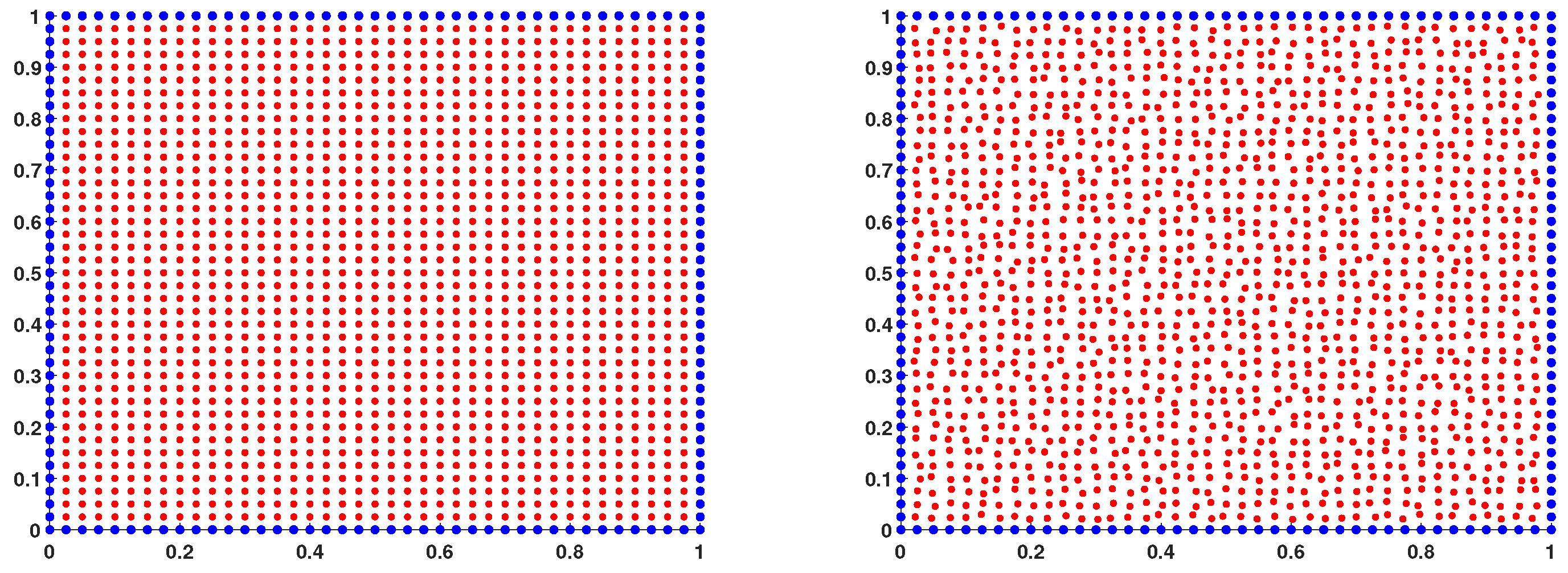
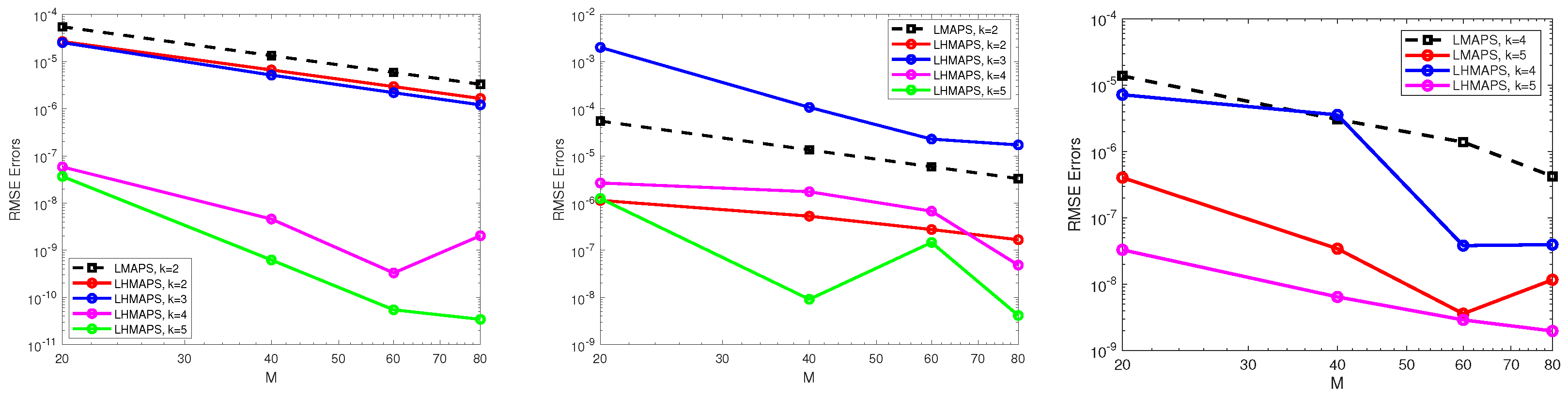
Example 1.

We consider problem (1) with $\mathcal{L}={\mathcal{L}}_{+}$, $\lambda =1$, and $\mathrm{\Omega }={(0,1)}^2$. The analytical solution is chosen to be $u=e^{x+y}$. Figure 1 shows examples of Cartesian nodes and unstructured notes. We also set the total number of Cartesian nodes N to be $M\times M$, with M denoting the number of nodes in each row and each column.

In this example, we first compute the numerical solutions of LMAPS and LHMAPS using polynomial basis functions of degree $k=2,3,4,5$, respectively, and compare their RMSEs in

Table 2. RMSE errors of LMAPS and LHMAPS using polynomials of degree $k=2,3,4,5$ and MQ with $m=5$.

M	LMAPS		LHMAPS
	$\mathit{k}=\mathbf{2}$		$\mathit{k}=\mathbf{2}$		$\mathit{k}=\mathbf{3}$		$\mathit{k}=\mathbf{4}$		$\mathit{k}=\mathbf{5}$
	${\mathit{E}}_{\mathit{RMSE}}$	Rate	${\mathit{E}}_{\mathit{RMSE}}$	Rate	${\mathit{E}}_{\mathit{RMSE}}$	Rate	${\mathit{E}}_{\mathit{RMSE}}$	Rate	${\mathit{E}}_{\mathit{RMSE}}$	Rate
20	$5.47\times {10}^{-5}$	-	$2.66\times {10}^{-5}$	-	$2.53\times {10}^{-5}$	-	$5.84\times {10}^{-8}$	-	$3.67\times {10}^{-8}$	-
40	$1.34\times {10}^{-5}$	2.03	$6.65\times {10}^{-6}$	1.99	$5.17\times {10}^{-6}$	2.29	$4.58\times {10}^{-9}$	3.67	$6.21\times {10}^{-10}$	5.88
60	$5.89\times {10}^{-6}$	2.02	$2.95\times {10}^{-6}$	2.00	$2.19\times {10}^{-6}$	2.11	$3.30\times {10}^{-10}$	6.48	$5.46\times {10}^{-11}$	6.00
80	$3.30\times {10}^{-6}$	2.01	$1.65\times {10}^{-6}$	2.02	$1.21\times {10}^{-6}$	2.06	$2.03\times {10}^{-9}$	−6.31	$3.42\times {10}^{-11}$	1.62

. In LHMAPS, we use the MQ radial basis functions centered at $m=5$ nearest nodes to the local center. It can be seen that LMAPS using structured stencils fails to produce a solution when $k>2$, since the matrices for computing local weights become singular. Therefore, we only list the RMSEs of LMAPS for $k=2$. However, when the Hermite interpolation is added in the local numerical scheme, the errors of LHMAPS using polynomial basis functions with $k=2,3,4,5$ converges as N increases.

Secondly, we test LHMAPS using polynomial basis functions and PS radial basis functions in the Hermite interpolation. To determine the appropriate order $\omega$ for the PS radial basis functions, we compute errors of LHMAPS solution obtained from a $20\times 20$ grid and select the order $\omega$ from orders 1–7 that minimizes the LHMAPS error (see

Table 3. RMSE errors of LHMAPS using polynomials of degree $k=2$ and PS of order $\omega =1,\cdots ,7$ when $M=20$ and $m=5$.

$\mathit{\omega }$	1	2	3	4	5	6	7
RMSE	$2.77\times {10}^{-4}$	$1.01\times {10}^{-4}$	$4.11\times {10}^{-5}$	$1.39\times {10}^{-5}$	$6.24\times {10}^{-7}$	$9.21\times {10}^{-6}$	$1.46\times {10}^{-5}$

). It is observed that the minimum of errors is achieved when $w=5$. Therefore, we present errors of LHMAPS using polynomial basis functions and PS radial basis functions of order $\omega =5$ in

Table 4. RMSE errors of LMAPS and LHMAPS using polynomials of degree $k=2,3,4,5$ and PS radial basis functions of order $\omega =5$ when $m=5$.

M	LMAPS		LHMAPS
	$\mathit{k}=\mathbf{2}$		$\mathit{k}=\mathbf{2}$		$\mathit{k}=\mathbf{3}$		$\mathit{k}=\mathbf{4}$		$\mathit{k}=\mathbf{5}$
	${\mathit{E}}_{\mathit{RMSE}}$	Rate	${\mathit{E}}_{\mathit{RMSE}}$	Rate	${\mathit{E}}_{\mathit{RMSE}}$	Rate	${\mathit{E}}_{\mathit{RMSE}}$	Rate	${\mathit{E}}_{\mathit{RMSE}}$	Rate
20	$5.47\times {10}^{-5}$	-	$1.14\times {10}^{-6}$	-	$2.00\times {10}^{-3}$	-	$2.67\times {10}^{-6}$	-	$1.25\times {10}^{-6}$	-
40	$1.34\times {10}^{-5}$	2.03	$5.27\times {10}^{-7}$	1.11	$1.07\times {10}^{-3}$	0.91	$1.74\times {10}^{-6}$	0.62	$9.11\times {10}^{-9}$	7.10
60	$5.89\times {10}^{-6}$	2.02	$2.75\times {10}^{-7}$	1.61	$2.27\times {10}^{-4}$	3.83	$6.73\times {10}^{-7}$	2.34	$1.46\times {10}^{-7}$	−6.84
80	$3.30\times {10}^{-6}$	2.01	$1.67\times {10}^{-7}$	1.72	$1.71\times {10}^{-4}$	0.98	$4.85\times {10}^{-8}$	9.14	$4.14\times {10}^{-9}$	12.38

, which shows a significant improvement compared to LMAPS.

In addition, we compute LMAPS and LHMAPS solutions using polynomial basis functions and multiquadric (MQ) radial basis functions with $m=5$ on unstructured nodes, as reported in

Table 5. RMSE errors of LMAPS using polynomials vs. LHMAPS using Poly + MQ with $m=5$ on unstructured nodes.

M	LMAPS				LHMAPS
	$\mathit{k}=\mathbf{4}$		$\mathit{k}=\mathbf{5}$		$\mathit{k}=\mathbf{4}$		$\mathit{k}=\mathbf{5}$
	${\mathit{E}}_{\mathit{RMSE}}$	Rate	${\mathit{E}}_{\mathit{RMSE}}$	Rate	${\mathit{E}}_{\mathit{RMSE}}$	Rate	${\mathit{E}}_{\mathit{RMSE}}$	Rate
20	$1.38\times {10}^{-5}$	-	$4.05\times {10}^{-7}$	-	$7.18\times {10}^{-6}$	-	$3.31\times {10}^{-8}$	-
40	$3.05\times {10}^{-6}$	2.1756	$3.44\times {10}^{-8}$	3.5586	$3.57\times {10}^{-7}$	4.3281	$6.46\times {10}^{-9}$	2.3567
60	$1.39\times {10}^{-6}$	1.9401	$3.61\times {10}^{-9}$	5.5633	$3.83\times {10}^{-8}$	5.5054	$2.91\times {10}^{-9}$	1.9625
80	$4.24\times {10}^{-7}$	4.1221	$1.17\times {10}^{-8}$	−4.0913	$3.96\times {10}^{-8}$	−0.1165	$1.98\times {10}^{-9}$	1.3404

, which confirms the better accuracy of LHMAPS. Here, we use unstructured node sets with $N=M^2$, where $M=20,40,60,80$, matching the corresponding Cartesian cases.

Lastly, Figure 2 plots the convergence behaviors of LMAPS and LHMAPS from Table 2, Table 4 and Table 5.

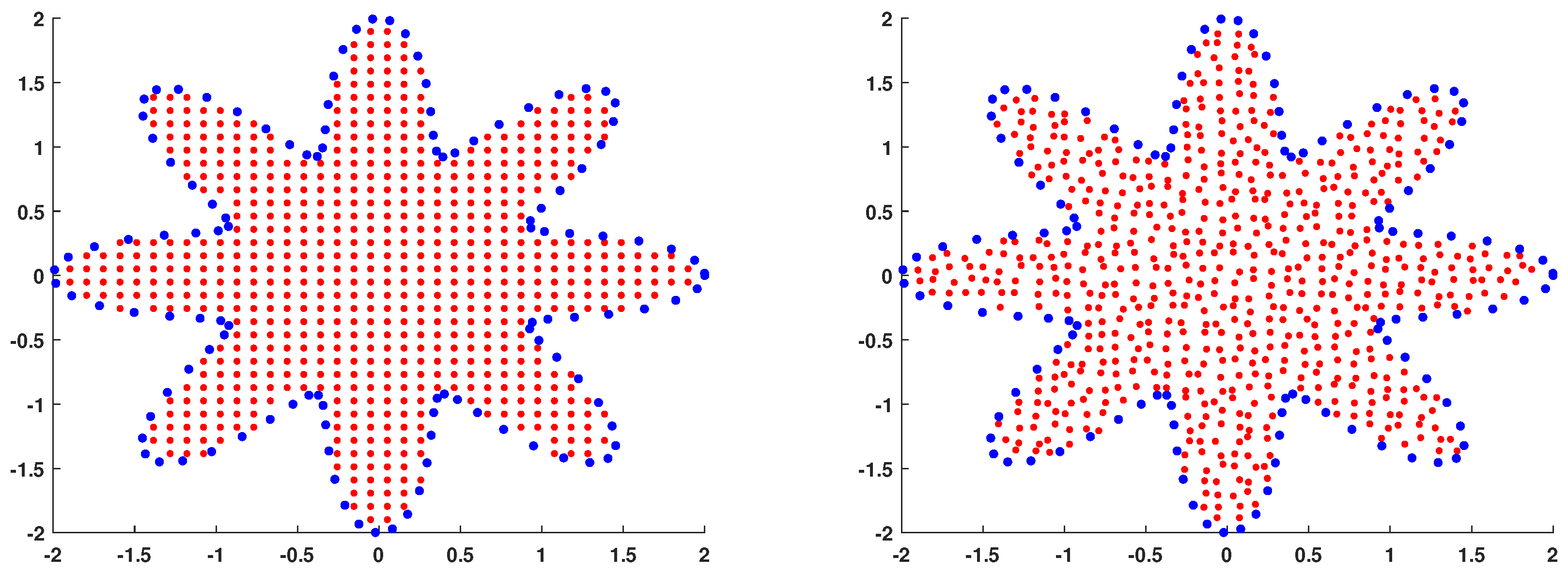
Example 2.

We consider problem (1) with $\mathcal{L}={\mathcal{L}}_{-}$ and $\lambda =10$ in the flower domain. The analytical solution is given by $u=sin\left({\displaystyle \frac{\pi x}{6}}\right)cos\left({\displaystyle \frac{3\pi y}{4}}\right)$. This domain Ω is defined to be the interior region of the closed curve $\rho =1+{cos}^2\left(4\theta \right)$ with $\mathsf{\partial }\mathrm{\Omega }=\left\{\right(x,y),x=\rho cos(\theta ),y=\rho sin(\theta ),0\le \theta \le 2\pi \}$.

Figure 3 shows examples of Cartesian nodes and unstructured notes distributed inside the flower domain. The boundary points are selected by partitioning $2\pi$ into $N_B$ equal parts and by setting ${\theta }_j={\displaystyle \frac{2(j-1)\pi }{N_B}}$ and $(x_j,y_j)=({\rho }_{j}cos{\theta }_j,{\rho }_{j}sin{\theta }_j)$ with ${\rho }_j=1+{cos}^2\left(4{\theta }_j\right)$ for any $j=1,\cdots ,N_B$.

In this example, we consider LHMAPS with several types of basis function combinations: polynomial basis functions combined with MQ radial basis functions for Hermite interpolation, polynomial basis functions combined with PS radial basis functions for Hermite interpolation, and PS radial basis functions combined with PS radial basis functions for Hermite interpolation.

First, we combine polynomial basis functions with MQ radial basis functions for Hermite interpolation in the LHMAPS scheme. Numerical results on Cartesian nodes are presented in

Table 6. RMSE errors of LHMAPS using polynomials of degree $k=2,3,4$ and MQ radial basis functions for Hermite interpolation with $m=5$.

N	LMAPS		LHMAPS
	$\mathit{k}=\mathbf{2}$		$\mathit{k}=\mathbf{2}$		$\mathit{k}=\mathbf{3}$		$\mathit{k}=\mathbf{4}$
	${\mathit{E}}_{\mathit{RMSE}}$	Rate	${\mathit{E}}_{\mathit{RMSE}}$	Rate	${\mathit{E}}_{\mathit{RMSE}}$	Rate	${\mathit{E}}_{\mathit{RMSE}}$	Rate
199	$1.75\times {10}^{-3}$	-	$1.79\times {10}^{-3}$	-	$1.94\times {10}^{-3}$	-	$8.03\times {10}^{-3}$	-
789	$1.99\times {10}^{-4}$	3.14	$1.55\times {10}^{-4}$	3.53	$1.51\times {10}^{-4}$	3.69	$1.52\times {10}^{-4}$	5.72
1689	$7.29\times {10}^{-5}$	2.58	$6.72\times {10}^{-5}$	2.15	$1.20\times {10}^{-4}$	0.58	$2.01\times {10}^{-6}$	11.14
3067	$2.56\times {10}^{-5}$	3.43	$2.16\times {10}^{-5}$	3.72	$2.90\times {10}^{-5}$	4.67	$2.95\times {10}^{-6}$	−1.26
4748	$3.35\times {10}^{-5}$	−1.20	$1.12\times {10}^{-5}$	2.94	$5.71\times {10}^{-6}$	7.28	$1.71\times {10}^{-6}$	2.44

. It is observed again that LMAPS works only for $k=2$, and LHMAPS improves the results of LMAPS by using additional MQ radial basis functions. Similar results are observed when using polynomial basis functions with PS radial basis functions for Hermite interpolation in the LHMAPS scheme, as shown in

Table 7. RMSE errors of LHMAPS using polynomials of degree 2 and PS radial basis functions of order $\omega =1,\cdots ,8$ when $N=199,m=4$.

$\mathit{\omega }$	1	2	3	4	5	6	7	8
$E_{RMSE}$	$6.81\times {10}^{-2}$	$9.32\times {10}^{-2}$	$1.04\times {10}^{-3}$	$1.36\times {10}^{-3}$	$5.20\times {10}^{-3}$	$7.26\times {10}^{-3}$	$3.80\times {10}^{-3}$	$3.91\times {10}^{-3}$

and

Table 8. RMSE errors of LMAPS and LHMAPS using polynomials of degree $k=2,\cdots ,4$ and PS radial basis functions with order $\omega =3$ when $m=4$.

N	LMAPS		LHMAPS
	$\mathit{k}=\mathbf{2}$		$\mathit{k}=\mathbf{2}$		$\mathit{k}=\mathbf{3}$		$\mathit{k}=\mathbf{4}$
	${\mathit{E}}_{\mathit{RMSE}}$	Rate	${\mathit{E}}_{\mathit{RMSE}}$	Rate	${\mathit{E}}_{\mathit{RMSE}}$	Rate	${\mathit{E}}_{\mathit{RMSE}}$	Rate
199	$1.76\times {10}^{-3}$	-	$1.046\times {10}^{-3}$	-	$8.806\times {10}^{-4}$	-	$1.036\times {10}^{-3}$	-
789	$1.99\times {10}^{-4}$	3.14	$1.37\times {10}^{-4}$	2.92	$1.41\times {10}^{-3}$	−0.68	$5.35\times {10}^{-5}$	4.27
1689	$7.29\times {10}^{-5}$	2.58	$5.07\times {10}^{-5}$	2.55	$5.78\times {10}^{-4}$	2.20	$1.35\times {10}^{-5}$	3.39
3067	$2.56\times {10}^{-5}$	3.43	$1.91\times {10}^{-5}$	3.21	$8.72\times {10}^{-5}$	6.57	$2.59\times {10}^{-5}$	−2.26
4748	$3.35\times {10}^{-5}$	−1.19	$1.67\times {10}^{-5}$	0.60	$1.32\times {10}^{-4}$	−1.87	$2.25\times {10}^{-6}$	10.94

. Table 7 compares the RMSEs of LHMAPS using polynomial basis functions of degree 2 and PS radial basis functions of order $\omega =1,\cdots ,8$ when $N=199$ and $m=4$. From this comparison, $\omega =3$ is selected for Hermite interpolation when $k=2$, $m=4$, with different N used to generate Table 8.

Secondly, we present the LMAPS results using PS radial basis functions of order $\omega =2$ with $n=9$ and of order $\omega =3$ with $n=13$ in

Table 9. RMSE errors of LMAPS and LHMAPS using PS2 and MQ with $n=9,m=4$ and PS3 with $n=13,m=9$.

N	LMAPS				LHMAPS
	PS2 ($\mathit{n}=\mathbf{9}$)		PS3 ($\mathit{n}=\mathbf{13}$)		PS2 ($\mathit{n}=\mathbf{9},\mathit{m}=\mathbf{4}$)		PS3 ($\mathit{n}=\mathbf{13},\mathit{m}=\mathbf{4}$)
	${\mathit{E}}_{\mathit{RMSE}}$	Rate	${\mathit{E}}_{\mathit{RMSE}}$	Rate	${\mathit{E}}_{\mathit{RMSE}}$	Rate	${\mathit{E}}_{\mathit{RMSE}}$	Rate
199	$2.05\times {10}^{-1}$	-	$3.06\times {10}^{-4}$	-	$4.98\times {10}^{-2}$	-	$1.16\times {10}^{-4}$	-
789	$5.12\times {10}^{-2}$	2.0007	$1.83\times {10}^{-5}$	4.0666	$6.38\times {10}^{-3}$	2.9648	$5.36\times {10}^{-6}$	4.4381
1689	$6.56\times {10}^{-2}$	−0.6109	$4.57\times {10}^{-6}$	3.4179	$1.50\times {10}^{-3}$	3.5755	$1.04\times {10}^{-6}$	4.0541
3067	$2.11\times {10}^{-2}$	3.9374	$2.16\times {10}^{-6}$	2.6081	$6.26\times {10}^{-4}$	3.0295	$3.11\times {10}^{-7}$	4.1828
4748	$5.36\times {10}^{-2}$	−4.1741	$1.24\times {10}^{-6}$	2.4923	$5.71\times {10}^{-4}$	0.4075	$1.35\times {10}^{-7}$	3.7388

. These results are compared with those of LHMAPS augmented by multiquadric (MQ) radial basis functions using $(\omega ,n,m)=(2,9,4)$ and $(\omega ,n,m)=(3,13,9)$, respectively. The results clearly indicate that incorporating Hermite interpolation into LMAPS leads to improved accuracy.

In addition, we apply the proposed LHMAPS to unstructured nodes as shown in the right plot of Figure 1.

Table 10. RMSE errors of LMAPS using polynomials vs. LHMAPS using polynomial basis functions of degree $k=2,3,4$ and MQ with $m=5$ on unstructured nodes.

N	LMAPS
	$\mathit{k}=\mathbf{2}$		$\mathit{k}=\mathbf{3}$		$\mathit{k}=\mathbf{4}$
	${\mathit{E}}_{\mathit{RMSE}}$	Rate	${\mathit{E}}_{\mathit{RMSE}}$	Rate	${\mathit{E}}_{\mathit{RMSE}}$	Rate
196	$7.40\times {10}^{-3}$	-	$2.40\times {10}^{-3}$	-	$7.44\times {10}^{-4}$	-
780	$1.32\times {10}^{-3}$	2.4917	$8.76\times {10}^{-4}$	1.4555	$2.05\times {10}^{-4}$	1.8617
1728	$4.83\times {10}^{-4}$	2.4702	$3.15\times {10}^{-4}$	2.5270	$3.18\times {10}^{-5}$	4.5960
3048	$9.52\times {10}^{-4}$	−2.3576	$1.23\times {10}^{-4}$	3.2633	$4.86\times {10}^{-6}$	6.5248
	LHMAPS
N	$k=2$		$k=3$		$k=4$
	$E_{RMSE}$	rate	$E_{RMSE}$	rate	$E_{RMSE}$	rate
196	$5.85\times {10}^{-3}$	-	$2.36\times {10}^{-3}$	-	$1.98\times {10}^{-3}$	-
780	$4.37\times {10}^{-4}$	3.7423	$5.58\times {10}^{-4}$	2.0831	$3.29\times {10}^{-4}$	2.5888
1728	$3.97\times {10}^{-4}$	0.2354	$1.93\times {10}^{-4}$	2.6222	$4.19\times {10}^{-3}$	−6.2773
3048	$2.25\times {10}^{-4}$	1.9851	$1.96\times {10}^{-4}$	−0.0661	$8.50\times {10}^{-5}$	13.5511

presents the comparison of LMAPS using polynomial basis functions of degrees $2,3,4$ and the corresponding LHMAPS using MQ radial basis functions in Hermite interpolation, which shows that the additional MQ polynomials are unnecessary.

Table 11. RMSE errors of LMAPS and LHMAPS using PS2 with $n=9,m=4$ and PS3 with $n=13,m=4$ on unstructured nodes.

N	LMAPS				LHMAPS
	PS2 ($\mathit{n}=\mathbf{9}$)		PS3 ($\mathit{n}=\mathbf{13}$)		PS2 ($\mathit{n}=\mathbf{9},\mathit{m}=\mathbf{4}$)		PS3 ($\mathit{n}=\mathbf{13},\mathit{m}=\mathbf{4}$)
	${\mathit{E}}_{\mathit{RMSE}}$	Rate	${\mathit{E}}_{\mathit{RMSE}}$	Rate	${\mathit{E}}_{\mathit{RMSE}}$	Rate	${\mathit{E}}_{\mathit{RMSE}}$	Rate
196	$3.61\times {10}^{-1}$	-	$2.63\times {10}^{-4}$	-	$5.72\times {10}^{-2}$	-	$1.40\times {10}^{-4}$	-
780	$2.34\times {10}^{-1}$	0.6271	$4.55\times {10}^{-5}$	2.5281	$1.22\times {10}^{-1}$	−1.0903	$1.11\times {10}^{-5}$	3.6592
1728	$6.98\times {10}^{-2}$	2.9835	$1.47\times {10}^{-5}$	2.7922	$2.12\times {10}^{-2}$	4.3100	$3.54\times {10}^{-6}$	2.8095
3048	$4.55\times {10}^{-1}$	−6.5149	$8.45\times {10}^{-6}$	1.9188	$4.23\times {10}^{-2}$	−2.3979	$1.64\times {10}^{-6}$	2.6695
4733	$4.74\times {10}^{-2}$	10.1364	$5.29\times {10}^{-6}$	2.0998	$1.86\times {10}^{-1}$	−6.6386	$8.84\times {10}^{-7}$	2.7727

presents the comparison between LMAPS using PS radial basis functions and its corresponding LHMAPS using PS radial basis functions in Hermite interpolation. It appears that adding the Hermite interpolation over a small-sized stencil of $n=9$ nodes to LMAPS does not show significant improvement on unstructured nodes when $\omega =2$, as it did on Cartesian nodes, which implies that a larger-sized stencil is more appropriate for unstructured nodes. These results show that LHMAPS using PS3 with $n=13$, $m=4$ achieves the highest accuracy on unstructured node sets.

6. Conclusions and Future Work

We propose LHMAPS for solving two-dimensional inhomogeneous Helmholtz-type equations using three types of combined basis functions: polynomial basis functions with MQ radial basis functions, polynomial basis functions with PS radial basis functions, and PS radial basis functions with MQ radial basis functions. This framework improves the local approximation of LMAPS by incorporating additional derivative information through Hermite interpolation and provides an alternative to compact finite difference methods for solving partial differential equations. The flexibility of coupling the LMAPS local scheme with different basis functions for Hermite interpolation broadens the range of localized RBF collocation approaches.

Numerical experiments were used to investigate different basis function combinations of LHMAPS and compare their performance with LMAPS. In both numerical experiments, LHMAPS consistently yielded substantial accuracy improvements over LMAPS on structured (Cartesian) grids, at the cost of only a slight increase in computational effort. However, on unstructured node sets, the performance of LHMAPS was less uniform and appeared to depend on the complexity of the computational domain, a behavior that warrants further investigation.

In future work, we plan to extend the proposed framework to anisotropic Helmholtz equations arising in geophysics and electromagnetics, as well as nonlinear Helmholtz equations encountered in plasma physics.