Evaluating the Impact of the Government Floor Price Policy (HPP) on Farm-Gate-Level Harvested Dry Paddy (GKP) Price Trends Through Machine Learning-Based Forecasting

Abstract

Government Purchasing Price (Harga Pembelian Pemerintah, HPP) is a policy established to maintain stable Harvested Dry Paddy (Gabah Kering Panen, GKP) prices at the farm-gate level and to protect farmers from declining incomes due to price drops during harvest periods. The effectiveness of the policy has yet to be evaluated; however, reports indicate that paddy prices in several regions are still below the HPP rate. This study explores variations in the trends and volatility of farm-gate-level GKP prices before and after the adoption of the new HPP policy and constructs a provincial-level forecasting model based on the Extreme Gradient Boosting (XGBoost) methodology using a daily provincial panel dataset covering the period from 1 January 2023 to 31 December 2025. An analysis of six sample provinces was performed: the Special Region of Yogyakarta (DIY), East Java, South Kalimantan, Bali, West Sumatra, and Jambi. The model was trained using pre-policy observations and recursively forecasted post-policy prices under a hypothetical no-HPP-policy scenario, which were then descriptively compared with observed prices after the policy was implemented. The results show that the model delivers very high prediction accuracy, with tested Mean Absolute Percentage Error (MAPE) values ranging from 0.61% to 1.60% and Root Mean Squared Error (RMSE) values ranging from IDR 50.31 to IDR 158.04. The comparison shows that observed post-policy GKP prices tend to remain higher and more stable over time than those forecasted under the no-HPP-policy scenario, although the magnitude of this difference varies among regions. These findings provide descriptive forecasting evidence regarding post-policy GKP price dynamics rather than definitive causal estimates of policy impact.

1. Introduction

One of the main pillars supporting the national economy, the agricultural sector, achieved performance growth during the first quarter of 2025, when rice production increased by 51.45% and corn production increased by 39.02% compared to the same period in the previous year [1]. The positive performance of this sector was supported by programs such as the modernization of agricultural equipment and machinery, improvements in irrigation quality, and growth in planting areas, which suggest that the government’s program to strengthen food security and increase agricultural productivity is beginning to yield results [2].

Although production conditions show a positive trend, empirical evidence shows that farmers are facing serious problems as a result of paddy prices falling below the Government Purchasing Price (Harga Pembelian Pemerintah, HPP). This pattern of insufficient returns at farm-gate-level paddy prices and of its potential negative impact on farmers’ welfare means that the harvest period, which should drive income improvements, instead represents a cause for concern [3].

This pressure is mainly felt by the vast majority of small-scale farmers, with approximately 68% controlling only one hectare or less of land and earning less than IDR 75,000 per day at best, an income barely enough to cover their households’ basic needs. Under conditions of low paddy prices, these small-scale farmers, who earn an average of IDR 44,507 per working day, become vulnerable to dire circumstances exacerbated by their limited access to land, credit, markets, and technology, which translates into a weak bargaining position when selling their harvests. Consequently, declining paddy prices limit their income, raise the risk of poverty, and create welfare disparities between smallholders and large producers [4].

This vulnerability becomes even more evident considering that the majority of farmers in key rice-producing regions are smallholders, a proportion that exceeds that of other types of agricultural investment in most areas. In Central Java, small-scale farmers account for more than 81% of producers, while the figure reaches 83.5% in West Java and nearly 88% in Banten. About 75% of farmers in East Java, the province with the highest paddy production, operate on a small scale. This shows that subsistence-based agriculture is still very common. Outside Java, smallholders make up about 60% of farmers in Lampung and about 64% in North Sumatra. On the other hand, provinces in which large-scale agribusiness is more common, like Riau and Jambi, have far fewer small-scale farmers, accounting for only only 37% to 39% of farmers. This pattern illustrates the economic challenges faced by many farmers. Low paddy prices tend to keep smallholders trapped in a cycle of poverty [4].

The establishment of the HPP policy for Harvested Dry Paddy (Gabah Kering Panen, GKP) at the farm-gate level at IDR 6500 per kilogram, along with the elimination of paddy price refraction, is intended to ensure that farmers receive fairer and more stable prices, especially during peak harvest periods when prices tend to decline. The policy seeks to enhance the protection of farmers while also supporting the achievement of national food self-sufficiency. The legal basis for this policy is the Decree of the Head of the National Food Agency No. 14/2025 on Amendment to Decree No. 2/2025 on Government Purchasing Price and Refraction of Paddy and Rice Prices (Harga Pembelian Pemerintah dan Rafaksi Harga Gabah dan Beras), which establishes a clean and measurable mechanism for paddy procurement in the field [5].

Based on the national daily price trends of GKP at the farm-gate level, as presented in Figure 1, it can be observed that prior to the establishment of the HPP policy, farm-gate-level GKP prices fluctuated and tended to remain below or around the HPP threshold, particularly following the sharp decline in mid-2024. Once the HPP policy was implemented, national price dynamics showed a continuous upward trend with less variability, such that post-policy prices were more likely to remain at or above the HPP threshold. The pattern suggests that the HPP policy helped maintain national price levels, as prices in the post-policy period seemed to remain higher than those recorded in the pre-policy period.

Regional reports, however, indicate that the HPP policy and its implementation mechanisms have yet to operate optimally at the farm-gate level. For example, in Banyuasin Regency, South Sumatra, the prices received by farmers only range from IDR 5300 to IDR 5800 per kilogram. A similar scenario has been reported in the Kulon Progo district, located in the Special Region of Yogyakarta, where farmers reported an average price of only IDR 5100 per kilogram, far below the HPP threshold. According to Yudi Indarto, the head of Mandiri Farmer Group in Kulon Progo, farmers’ paddy is often purchased by middlemen at low prices without intervention from BULOG, causing prices to fall to IDR 3500–4000 per kilogram. Farmers are forced to accept such prices because of limited bargaining power, urgent daily economic needs, and insufficient BULOG absorption. These findings show that there is a gap between policy design and implementation in the field. This suggests that the goal of the HPP policy to protect farmers’ incomes has not yet been fully achieved [6].

Previous studies have investigated the effectiveness of the HPP policy from different perspectives. Nainggolan and Soetjipto (2016) analyzed the effectiveness of HPP using an econometric 2SLS framework and found that the policy affected farm-gate-level GKP prices with a time lag [7]. Meanwhile, Suparmin et al. (2022) showed that HPP contributed to price stability in Lombok, although seasonal production patterns and market conditions continued to influence price movements [8]. However, these studies primarily relied on conventional statistical approaches, annual or monthly observations, and specific regional or national settings, which may limit their ability to capture nonlinear daily price dynamics and regional heterogeneity under the new HPP regime.

Despite these findings, previous studies relied on earlier HPP policy settings and mainly focused on direct evaluations of policy effectiveness. Under the current HPP framework, farm-gate-level GKP prices in several regions still occasionally fall below the HPP threshold. A policy brief published by the Institute for the Development of Economics and Finance (INDEF, 2025) also highlighted that the implementation of a uniform HPP regardless of grain quality may increase market vulnerability and price instability [9]. In addition, previous studies have paid limited attention to forecasting-based descriptive scenarios under hypothetical no-policy conditions, particularly in capturing regional price dynamics and nonlinear price movements influenced by seasonal patterns, weather conditions, and market shocks. Therefore, this study examines the trends and volatility of farm-gate-level GKP prices before and after the implementation of the new HPP policy across selected provinces in Indonesia using province-level Extreme Gradient Boosting (XGBoost) forecasting models. The models are trained using pre-policy observations and used to forecast post-policy prices under a hypothetical no-HPP-policy scenario, which are then descriptively compared with observed post-policy prices.

Previous studies have shown that XGBoost is effective in capturing nonlinear relationships and complex temporal patterns in forecasting problems. Abubakar et al. (2025) reported that XGBoost outperformed LSTM in food-price forecasting across multiple evaluation metrics, demonstrating its strong predictive performance and stability [10]. In addition, Toharudin et al. (2023) highlighted the computational efficiency and flexibility of boosting algorithms in handling complex data structures [11]. A literature review by Kontopoulou et al. (2023) further noted that although classical models such as ARIMA are generally more interpretable, they may be less effective in representing nonlinear data behavior [12]. These findings suggest that XGBoost provides a suitable approach for modeling the nonlinear and volatile dynamics of farm-gate-level GKP prices under the current policy.

2. Materials and Methods

2.1. Purposive Sampling

Purposive sampling, also referred to as judgmental or expert sampling, constitutes a non-probability sampling method [13]. In this method, the units of analysis are chosen based on criteria established before the sampling process starts. The purpose of these criteria is to ensure that the selected units possess characteristics relevant to the research goals. The selection relies on the researcher’s discretion in identifying units that meet these criteria; consequently, the resulting sample aims to provide meaningful insights into the phenomenon under investigation rather than to statistically represent the entire population [14, 15].

Several strategies can be used to apply purposive sampling. Criterion sampling is one such method. It involves choosing units of analysis based on clearly defined criteria that align with the research objectives. Once the criteria are established, potential units can be identified through available data sources, official reports, or other relevant information. Another approach is maximum variation sampling, which involves selecting units that reflect diverse conditions or characteristics related to the phenomenon under study in order to illustrate the range of situations present within the data. In addition, theoretical sampling may be used in certain studies, whereby the selection of additional cases evolves during the analytical process as the researcher seeks to deepen the conceptual understanding of the phenomenon being examined [15].

2.2. Data Collection

The data used in this study are secondary data in the form of a daily provincial panel dataset of Harvested Dry Paddy (Gabah Kering Panen, GKP) producers at the farm-gate level. The data were collected for the period from 1 January 2023 to 31 December 2025 and were obtained from the official website of the Price Panel of the National Food Agency (Badan Pangan Nasional, Bapanas) [16]. Data collection was conducted at the provincial level. However, not all provinces in Indonesia were included. Only provinces that met the predefined sampling criteria were selected for analysis.

2.3. Data Splitting

In this study, dataset partitioning was carried out to objectively benchmark forecast accuracy using data not employed in model development. Accordingly, 14 January 2025 was used as the cutoff date based on the implementation of the HPP policy, and the data were divided into training data (for model building) and testing data. The training data were used to fit the forecasting model, while the testing data were used to assess its out-of-sample performance. The data were divided into training and testing sets using an 80:20 ratio to reduce overfitting and enable the model to generalize to unseen data [17]. Data from 15 January 2025 to 31 December 2025 were excluded from the model development stage and instead used for policy evaluation through a comparison of observed prices with model-reference prices under a hypothetical scenario in which the HPP policy was absent.

2.4. Extreme Gradient Boosting (XGBoost)

Machine learning is a key branch of artificial intelligence (AI) that possesses adaptive capabilities [18]. In recent years, with the development of machine learning approaches, time-series forecasting methods have been widely used as an effective means of addressing data complexity, including hidden internal patterns, outliers and noise, and variations in characteristics across domains, periods, and fields of data collection. This is in contrast with traditional time-series forecasting approaches, which often struggle to identify complex patterns due to their reliance on predefined linear relationships, while machine learning does not require such assumptions because it learns nonlinear patterns directly from the data [19].

One group of methods within machine learning is tree-based machine learning (TBML). These algorithms include several implementations, such as Random Forest, Gradient-Boosted Decision Trees (GBDT), and more recent methods like XGBoost, LightGBM, and CatBoost. Ensemble learning is a common strategy in TBML based on the “no free lunch” theorem, which states that no single algorithm is consistently superior to all others across all types of problems [20]. Ensemble learning differs from traditional methods that generate a single hypothesis from the training data. Instead, it combines two or more models (or learners) to produce predictions that are more accurate than those generated by a single model and to help prevent overfitting. This method is widely used in supervised learning for predictive tasks. In addition, TBML is computationally efficient, relatively easy to optimize, and competitive with deep learning approaches [21].

XGBoost is a boosting-based ensemble learning approach introduced by Chen and Guestrin in 2016 that has become a benchmark for evaluating the performance and scalability of machine learning algorithms [22]. As a gradient-boosting algorithm, XGBoost builds models sequentially in a forward stage-wise manner, with each iteration involving the training and addition of a weak learner (a decision tree) that attempts to minimize the residual errors of previous predictions [21, 22]. The learning process is expressed as the minimization of an objective function, which includes loss functions to improve predictive accuracy and regularization terms to limit model complexity [22]. Through its boosting mechanism and the weighted aggregation of all trees, XGBoost can generate a strong learner with high accuracy and stable predictive performance in both classification and regression problems [21].

As a comprehensive and systematic algorithm, XGBoost was developed through a series of technical improvements aimed at addressing scalability and computational efficiency issues commonly encountered in general tree-boosting methods. Among its most important features are a built-in mechanism for handling missing values and an approximate tree-learning method that uses the weighted quantile sketch technique, which is supported by a strong theoretical foundation. By considering the importance of each instance during the learning process, this approach also allows the model to better manage imbalanced datasets. In addition, a cache-aware block layout further optimizes memory access by storing data in a compressed column-based representation. By integrating these three innovations, XGBoost achieves both high accuracy and computational efficiency, allowing it to scale effectively to very large datasets while maintaining relatively low computational costs [22]. The architecture of the XGBoost model is presented in Figure 2 [23].

2.4.1. Feature Engineering

XGBoost, which is based on decision tree models, inherently lacks the built-in capability to capture temporal dependencies and therefore cannot directly model time sequences. Consequently, the performance of this model is highly dependent on the feature engineering process, which transforms time-series data into a supervised learning format, with the constructed features presented in

Table 1. Feature engineering for the Extreme Gradient Boosting (XGBoost) model.

Feature	Description
Date-Time	Used to extract calendar-based temporal information, including year, month, day, and hour.
Lag	Used to represent values from previous periods in both the short and long term.
Rolling-Window Statistics	Used to obtain information about trends and the degree of data fluctuation by calculating the mean or standard deviation over a specific time range.
Cyclical Encoding	Used to create seasonal features from time indices through calendar encoding or sine-cosine transformations.

[24].

2.4.2. XGBoost Modeling

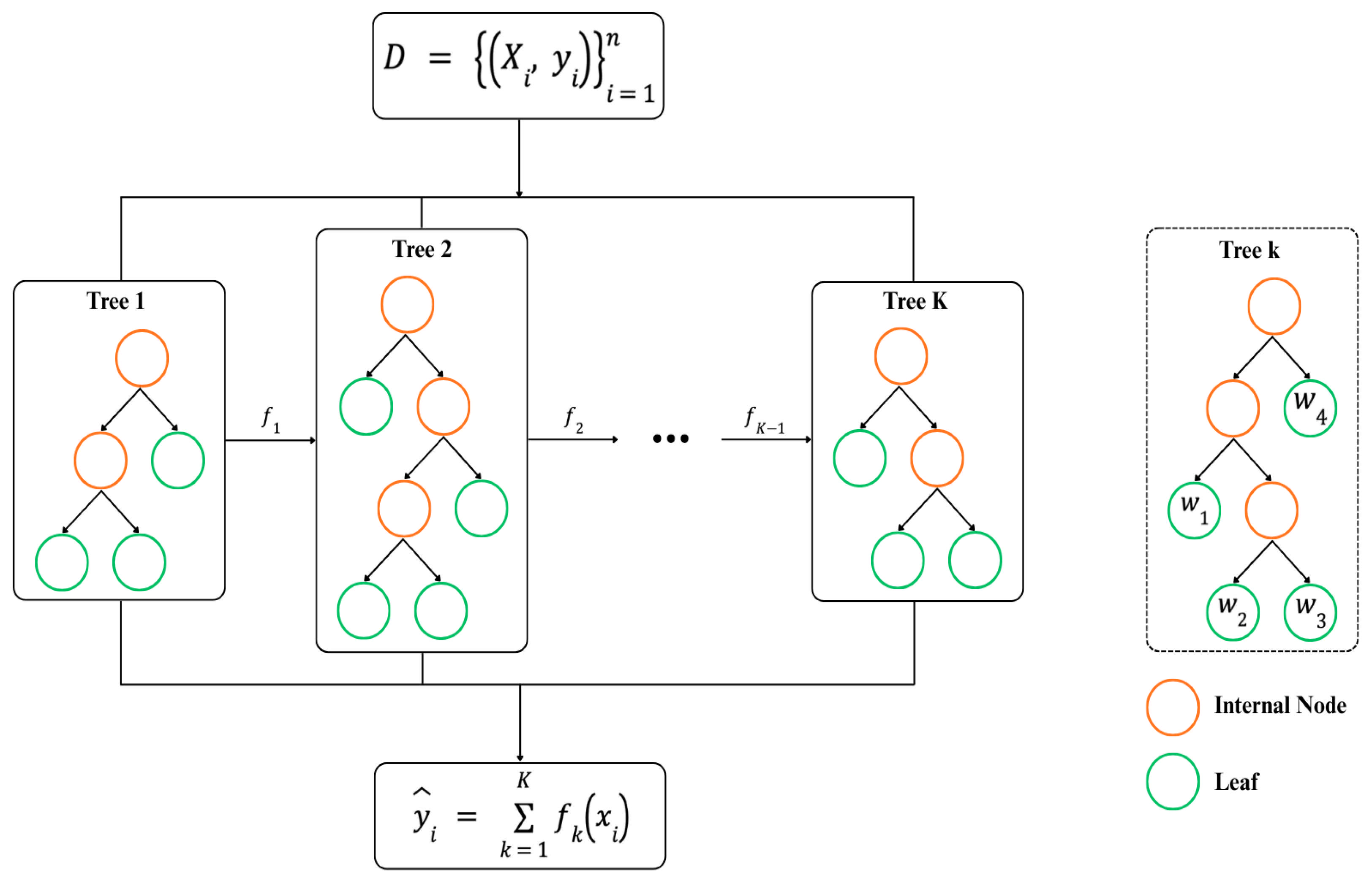
XGBoost is a boosting-based ensemble learning algorithm in which the predictive model is constructed from a combination of multiple decision trees [22]. The prediction of the decision tree ensemble model for the $i$-th input $x$ is defined as follows [25]:

$${\widehat{y}}_i={\displaystyle \sum _{k=1}^K}{f}_k\left(x_i\right),f_k\in F$$

(1)

with

$$F=\left\{f\left(x\right)={\omega }_{q\left(x\right)}\right\}\left(q:R^m\to \omega \in R^T\right)$$

(2)

where ${\widehat{y}}_i$ denotes the predicted value for the $i$-th observation, $K$ represents the number of decision trees constructed as weak learners, and $f_k$ denotes the $k$-th decision tree. The vector $x_i$ represents the input features for the $i$-th observation and has dimension $m$. Furthermore, $F$ denotes the space of regression tree functions, $\omega$ represents the weights assigned to each tree leaf, $q$ denotes the tree structure that maps each data point to a leaf index, and $T$ indicates the number of leaves in each tree.

Each regression tree partitions the feature space into several leaf nodes, where each leaf is associated with a prediction score. The function $q$ assigns each observation to a specific leaf node based on its feature values, while the corresponding leaf weight $\omega$ represents the prediction contribution generated by that leaf. The final prediction is obtained by summing the prediction contributions from all trees in the ensemble. Through this additive tree structure, XGBoost is able to capture complex nonlinear relationships and interactions among variables [25].

The objective function used in XGBoost training is a combination of a loss function and a regularization term that controls model complexity to avoid overfitting and is defined as follows [22]:

$$L\left(\varphi \right)={\displaystyle \sum _{i=1}^n}l\left(y_i,{\widehat{y}}_i\right)+{\displaystyle \sum _{k=1}^K}\Omega \left(f_k\right)$$

(3)

where $L\left(\varphi \right)$ denotes the objective function to be minimized, $n$ represents the number of observations, and $y_i$ is the actual value of the $i$-th observation. The function $l\left(y_i,{\widehat{y}}_i\right)$ serves as the loss function, while $\Omega \left(f_k\right)$ represents the regularization term.

In this study, the loss function employed is the Mean Squared Error (MSE), which measures the average of the squared differences between the actual values and the predicted values produced by the XGBoost model. The MSE is intended to impose a higher penalty on prediction errors of greater magnitude, thereby encouraging the model to generate more accurate predictions [25].

$$MSE={\displaystyle \frac{1}{n}}{\displaystyle \sum _{i=1}^n}{\left|y_i-{\widehat{y}}_i\right|}^2$$

(4)

Furthermore, the objective function in XGBoost includes a regularization term that helps prevent overfitting by controlling model complexity and penalizing overly complex decision trees, thereby contributing to better model generalization [25].

$$\Omega \left(f\right)=\gamma T+{\displaystyle \frac{1}{2}}\lambda {\left|\left|\omega \right|\right|}^2$$

(5)

where $\gamma$ is the penalty coefficient for adding leaf nodes, $\lambda$ is the penalty coefficient for leaf weights (L2 regularization factor), and $\omega$ is the weight value (score) of each leaf.

XGBoost builds the model in a stage-wise manner through an iterative process, which can be substituted into the objective function as shown in the following equations [25]:

$${\displaystyle {\widehat{y}}_i^{\left(t\right)}}={\displaystyle {\widehat{y}}_i^{\left(t-1\right)}}+{\eta f}_t\left(x_i\right)$$

(6)

$$L^{\left(t\right)}={\displaystyle \sum _{i=1}^n}l\left(y_i,{\displaystyle {\widehat{y}}_i^{\left(t-1\right)}}+f_t\left(x_i\right)\right)+\Omega \left(f_t\right)$$

(7)

where ${\displaystyle {\widehat{y}}_i^{\left(t\right)}}$ denotes the prediction at the $t$-th iteration, ${\displaystyle {\widehat{y}}_i^{\left(t-1\right)}}$ is the prediction at the $\left(t-1\right)$-th iteration, $\eta$ is the learning rate parameter, and $f_t\left(x_i\right)$ represents the newly added tree.

To accelerate convergence and improve model predictive accuracy, the objective function at each iteration is approximated using a second-order Taylor expansion. This approach yields a new optimization formulation involving the first-order and the second-order gradient of the loss function [25].

$$g_i={\partial }_{{\widehat{y}}^{\left(t-1\right)}}l\left(y_i,{\displaystyle {\widehat{y}}_i^{\left(t-1\right)}}\right)$$

(8)

$$h_i={\displaystyle {\partial }_{{\widehat{y}}^{\left(t-1\right)}}^2}l\left(y_i,{\displaystyle {\widehat{y}}_i^{\left(t-1\right)}}\right)$$

(9)

where $g_i$ represents the first-order gradient, indicating the direction and magnitude of the prediction error, and $h_i$ denotes the second-order Hessian, which measures the curvature or sensitivity of the loss function with respect to the predicted values. These quantities are incorporated into the optimization process through the second-order Taylor expansion approximation, enabling XGBoost to efficiently minimize the objective function and determine the optimal tree structure and leaf weights during the boosting process [25].

After applying the second-order Taylor expansion, the objective function at the t-th iteration can be expressed as follows:

$$L^{\left(t\right)}\simeq {\displaystyle \sum _{i=1}^n}l\left(y_i,{\displaystyle {\widehat{y}}_i^{\left(t-1\right)}}+{g_{i}f}_t\left(x_i\right)+{\displaystyle \frac{1}{2}}{h}_i{\displaystyle f_t^2}\left(x_i\right)\right)+\Omega \left(f_t\right)$$

(10)

The constant terms in the objective function can be omitted, allowing the objective function at the t-th iteration to be reformulated as the optimization target for constructing a new tree, as expressed in the following equation [25]:

$$L^{\left(t\right)}={\displaystyle \sum _{i=1}^n}\left[{g_{i}f}_t\left(x_i\right)+{\displaystyle \frac{1}{2}}{h}_i{\displaystyle f_t^2}\left(x_i\right)\right]+\Omega \left(f_t\right)$$

(11)

Next, by defining the set of data in the $j$-th leaf as $I_j=\left\{i|q\left(x_i\right)=j\right\}$ , and by substituting $f_t\left(x_i\right)$ based on the tree structure while expanding the regularization components, the objective function can be expressed in terms of the gradient contributions and leaf weights, together with a penalty on tree complexity, as follows [25]:

$$L^{~\left(t\right)}={\displaystyle \sum _{i=1}^n}\left[{g_{i}f}_t\left(x_i\right)+{\displaystyle \frac{1}{2}}{h}_i{\displaystyle f_t^2}\left(x_i\right)\right]+\gamma T+{\displaystyle \frac{1}{2}}\lambda {\displaystyle \sum _{j=1}^T}{\displaystyle {\omega }_j^2}$$

(12)

$$L^{~\left(t\right)}={\displaystyle \sum _{j=1}^T}\left[\left({\displaystyle \sum _{i\in I_j}}{g}_i\right){\omega }_j+{\displaystyle \frac{1}{2}}\left({\displaystyle \sum _{i\in I_j}}{h}_i+\lambda \right){\displaystyle {\omega }_j^2}\right]+\gamma T$$

(13)

Based on this formulation, the optimal weight for each leaf can be determined by setting the derivative equal to zero [25].

$${\displaystyle {\omega }_j^{\ast }}=-{\displaystyle \frac{{\displaystyle {\sum }_{i\in I_j}}{g}_i}{{\displaystyle {\sum }_{i\in I_j}}{h}_i+\lambda }}$$

(14)

Using these optimal weights, the minimum value of the objective function for a given tree structure can be computed and subsequently used as a scoring function to evaluate the quality of the resulting decision tree structure [25].

$$L^{~\left(t\right)}\left(q\right)=-{\displaystyle \frac{1}{2}}{\displaystyle \sum _{j=1}^T}{\displaystyle \frac{{\left({\displaystyle {\sum }_{i\in I_j}}{g}_i\right)}^2}{{\displaystyle {\sum }_{i\in I_j}}{h}_i+\lambda }}+\gamma T$$

(15)

When all observations are present at a single node $I$ , the value of the objective function for that node can be expressed as follows [22]:

$$L=-{\displaystyle \frac{1}{2}}{\displaystyle \frac{{\left({\displaystyle {\sum }_{i\in I}}{g}_i\right)}^2}{{\displaystyle {\sum }_{i\in I}}{h}_i+\lambda }}+\gamma$$

(16)

Based on the optimal leaf weights obtained from the optimization process, the objective function can be rewritten in a simplified form that depends only on the aggregated gradients and Hessians of the observations within a node. After determining the optimal weight for each leaf, the next step in constructing the tree is to evaluate possible splits at each node. This evaluation is performed by measuring the gain produced by a split, which represents the reduction in the loss function achieved by splitting the node compared to leaving it unsplit. Let $I_L$ and $I_R$ denote the sets of data in the left and right child nodes after the split, and let $I=I_L\cup I_R$ denote the set of data in the parent node; then, the loss reduction resulting from the split can be expressed as follows [22]:

$$L_{after split}=-{\displaystyle \frac{1}{2}}{\displaystyle \frac{{\left({\displaystyle {\sum }_{i\in I_L}}{g}_i\right)}^2}{{\displaystyle {\sum }_{i\in I_L}}{h}_i+\lambda }}-{\displaystyle \frac{1}{2}}{\displaystyle \frac{{\left({\displaystyle {\sum }_{i\in I_R}}{g}_i\right)}^2}{{\displaystyle {\sum }_{i\in I_R}}{h}_i+\lambda }}+2\gamma$$

(17)

$$L_{split}={\displaystyle \frac{1}{2}}\left[{\displaystyle \frac{{\left({\displaystyle {\sum }_{i\in I_L}}{g}_i\right)}^2}{{\displaystyle {\sum }_{i\in I_L}}{h}_i+\lambda }}+{\displaystyle \frac{{\left({\displaystyle {\sum }_{i\in I_R}}{g}_i\right)}^2}{{\displaystyle {\sum }_{i\in I_R}}{h}_i+\lambda }}-{\displaystyle \frac{{\left({\displaystyle {\sum }_{i\in I}}{g}_i\right)}^2}{{\displaystyle {\sum }_{i\in I}}{h}_i+\lambda }}\right]-\gamma$$

(18)

A node will split only if the candidate split has a gain greater than zero, indicating that after the split, the loss is reduced. Further, the splitting criterion also takes the regularization parameters (regularized weight) into account, such that splitting is beneficial only when the gain exceeds a specified threshold value. This condition aims to avoid the creation of unnecessarily complex tree structures and to maintain the generalization capability of the model [22].

2.4.3. Hyperparameter Tuning

Hyperparameter tuning greatly affects the performance of the constructed model. Unlike parameters that are automatically estimated by the algorithm, in the XGBoost model, hyperparameters are set by the researcher to control the learning process. Therefore, hyperparameter tuning is essential for achieving more accurate predictions.

Table 2. Hyperparameter settings for the XGBoost model.

Parameter	Type	Range	Description
colsample_bytree	floating-point	(0, 1]	The proportion of features used to build each tree (default = 1)
learning_rate	floating-point	[0, 1]	Step size for each iteration during objective function optimization (default = 0.3)
max_depth	integer	[0, $\infty$ )	The maximum depth of each tree (default = 6)
subsample	floating-point	(0, 1]	The proportion of data used to build each tree (default = 1)
min_child_weight	integer	[0, $\infty$ )	The minimum instance weight required for a child node (default = 1)
n_estimators	integer	[0, $\infty$ )	The maximum number of gradient-boosted trees to be built (default = 100)
gamma (min_split_loss)	floating-point	[0, $\infty$ )	The minimum loss reduction required to create a new partition on a leaf node (default = 0)
alpha (reg_alpha)	floating-point	[0, $\infty$ )	The L1 regularization parameter on the weights (default = 0)
lambda (reg_lambda)	floating-point	[0, $\infty$ )	The L2 regularization parameter on the weights (default = 1)

shows the hyperparameter settings used [26].

Grid search is a hyperparameter optimization technique that searches through all defined combinations of values for each hyperparameter to identify the configuration that results in the best model performance. This method is typically paired with time-series k-fold cross-validation to ensure the stability of results and the generalization capability of the model [27]. The approach partitions the dataset into $k$ non-overlapping subsets and calculates the average performance metric across all training iterations. The model is trained on $k-1$ subsets and tested on the remaining subset in each iteration. This process is repeated $k$ times, and each subset is used once as validation data [28].

2.5. Metric Evaluation

Evaluation metrics are quantitative measures used to assess how well a model makes predictions and performs on unseen data. These metrics allow an objective evaluation of model performance and facilitate comparison with other models or algorithms. The selection of appropriate evaluation metrics depends strongly on the problem context, the characteristics of the data, and the research objectives [29]. In this study, model evaluation was conducted using Root Mean Squared Error (RMSE) and Mean Absolute Percentage Error (MAPE).

2.5.1. Root Mean Squared Error (RMSE)

Root Mean Squared Error (RMSE) is an evaluation metric used to measure the average magnitude of error between predicted values and actual values and is calculated as the square root of the Mean Squared Error (MSE). RMSE represents the average vertical distance between actual values and predicted values from the fitted model, where errors are squared so that positive and negative deviations do not cancel each other out and larger errors are given greater weight [30, 31].

$$RMSE=\sqrt{{\displaystyle \frac{1}{n}}{\displaystyle \sum _{i=1}^n}{\left(y_i-{\widehat{y}}_i\right)}^2}$$

(19)

where $n$ denotes the number of observations, $y_i$ represents the $i$-th actual value, and ${\widehat{y}}_i$ represents the $i$-th predicted value.

RMSE values range from 0 to infinity, where smaller values indicate higher prediction accuracy, and a value of 0 indicates a perfect model. Unlike MSE, which is expressed in squared units of the original data, RMSE retains the same units as the original data, making it easier to interpret in the context of the analyzed problem [31].

2.5.2. Mean Absolute Percentage Error (MAPE)

To compare predictive performance across different units of measurement, unit-free evaluation metrics are required. Therefore, percentage-based metrics are more appropriate because they do not depend on specific measurement units [30]. Mean Absolute Percentage Error (MAPE) measures prediction accuracy by calculating the average of the absolute percentage differences between the predicted values and the actual observations. This metric expresses prediction errors in percentage terms, making it easier to assess how closely model predictions align with observed data [31].

$$MAPE={\displaystyle \frac{1}{n}}{\displaystyle \sum _{i=1}^n}\left|{\displaystyle \frac{y_i-{\widehat{y}}_i}{y_i}}\right|\times 100\%$$

(20)

A MAPE value below 10% indicates highly accurate predictions. Values between 10% and 20% indicate good accuracy, values between 20% and 50% are considered acceptable or reasonable, and values above 50% indicate poor predictive performance [32].

2.6. Feature Importance

Feature importance is a method for improving model interpretability by identifying which features have the greatest influence on predicted values [33]. The XGBoost model evaluates feature importance based on the reduction in impurity achieved during node splitting. These contributions are then aggregated across all decision trees in the model. The resulting scores improve model interpretability, support feature selection, and enable researchers to better understand the main factors influencing prediction results [34].

3. Methodology

Using the XGBoost method, this study predicted GKP prices at the farm-gate level. The analysis unit in this study consisted of provinces selected through purposive sampling. The research process included data collection, data splitting, feature engineering, hyperparameter tuning, model evaluation using relevant performance metrics, and feature importance analysis. The trained model was then used to predict farm-gate-level GKP prices under a hypothetical no-HPP-policy scenario for use in policy evaluation. Figure 3 illustrates the entire research workflow.

This study began with data collection, whereby the research data were organized at the provincial level, with provinces selected through purposive sampling. The data were then divided according to the cutoff date of HPP implementation, with only data prior to 15 January 2025 being used for model development. These data were then split into 80% training and 20% testing sets to construct an optimal model and assess its performance. Feature engineering was then applied to construct and transform features capable of capturing temporal patterns in the data. The same procedure was applied to both the training and testing sets. Predictive modeling was then carried out using the primary framework of this study, XGBoost.

To enhance model performance, hyperparameters were optimized through a grid search cross-validation approach, which evaluated various combinations of hyperparameter values to improve model performance. Through this process, the optimal hyperparameter configuration was identified and used to construct the final model. The best-performing model was then used to compare the predicted values with the actual values in the testing set using the RMSE and MAPE metrics to assess predictive accuracy and reliability. In addition, feature importance analysis was conducted to identify the variables that contributed most significantly to price predictions.

The next step involved predicting prices from 15 January 2025 onward using the model trained on pre-policy data. The forecasts were generated under a hypothetical scenario in which the HPP policy had not yet been implemented. Finally, a comparison was conducted between the actual prices and the forecasted prices under the no-HPP-policy scenario to evaluate the role of the policy in maintaining the stability of farm-gate-level GKP prices.

4. Results and Discussion

4.1. Results of Purposive Sampling

This study employed purposive sampling with a criterion-sampling approach to select the units of analysis (Indonesian provinces), based on criteria reflecting indications of ineffective implementation of the HPP policy, as evidenced in official reports and media coverage. To capture interregional variability, the selection process also incorporated the principle of maximum variation sampling by including provinces that were not necessarily expected to experience such issues as comparison units. Based on these criteria, several provinces were selected, the details of which are presented in

Table 3. Units of analysis based on purposive sampling selection.

Province	Sampling Approach	Selection Rationale	Source
Special Region of Yogyakarta (DIY)	Criterion	The price of paddy in Kulon Progo was reported as being IDR 5100 per kilogram.	Statement made by the head of the Independent Farmers Group in Kulon Progo, as reported by national media.
East Java	Criterion	The price of paddy in Jember ranged from IDR 6000 to IDR 6300 per kilogram.	Statement made by the Chair of the National Food Farmers Association was reported by national media.
South Kalimantan	Criterion	The price of paddy in Barito Kuala was reported as being IDR 5000 per kilogram.	Statement made by a farmer from Sungai Gampa Village, as reported in an official government publication.
Bali	Maximum Variation	The price of paddy in Tabanan was reported as being IDR 6500 per kilogram.	Statement made by I Gede Wirantaja, a farmer from Subak Aseman VI, as reported by national media.
West Sumatra	Maximum Variation	The highest reported price of paddy was IDR 7331 per kilogram.	Statement made by the Director of Vegetables and Medicinal Plants at the Ministry of Agriculture, as reported by national media.
Jambi	Maximum Variation	A total of 4620 tons of paddy were procured at a price of IDR 6500 per kilogram by BULOG.	Statement made by the Regional Head of BULOG’s Jambi Regional Office, as reported by national media.

.

4.2. Results of Data Splitting

The data used in this study consisted of farm-gate-level GKP prices collected at the provincial level. Based on the results of purposive sampling according to the predetermined criteria, six provinces were selected as the research sample: the Special Region of Yogyakarta (DIY), East Java, South Kalimantan, Bali, West Sumatra, and Jambi.

Data up to 14 January 2025, representing the period prior to the implementation of the HPP policy, were used for model development and were divided into training and testing sets in proportions of 80% and 20%, respectively. Meanwhile, data from 15 January 2025 to 31 December 2025 were used as the policy evaluation period. In total, the dataset used in this study comprised 1096 observations. The dataset partition used in this study for each provincial model is presented in

Table 4. Data splitting summary.

Data Type	Total Observations
Training Data	596
Testing Data	149
Policy Evaluation	351

.

During the policy evaluation period, post-policy forecasts under the hypothetical no-HPP-policy scenario were generated recursively, where temporal features were updated sequentially at each forecasting step to preserve the temporal structure of the data and avoid information leakage from post-policy observations.

4.3. Results of Feature Engineering

In the modeling process using the XGBoost method, models were developed separately for each sample province using the modeling dataset that had been divided into training and testing data. The features constructed for each provincial model were identical. The details of the features and the values used are presented in

Table 5. Features and values used in feature engineering.

Feature		Description
Date-Time	day	Day of the observation date.
	month	Month of the observation date.
	year	Year of the observation date.
	dayofweek	Day of the week of the observation date.
	dayofyear	Ordinal day within the year.
Lag	target_lag_k	Value of the target variable at $k$ previous periods.
Rolling-Window Statistics	col_mean_w	Represents the average trend calculated over a window of $w$ periods.
	col_std_w	Represents the level of fluctuation or variability calculated over a window of $w$ periods.
Cyclical Encoding	month_sin	Cyclical transformation used to represent monthly seasonal patterns.
	month_cos
	dayofweek_sin	Cyclical transformation used to represent weekly patterns.
	dayofweek_cos
	dayofyear_sin	Cyclical transformation used to represent annual patterns.
	dayofyear_cos

.

In this study, lag features and rolling-window statistics were constructed for each provincial model using time horizons of 3, 5, and 7 days. The selected values represent price information from preceding periods across multiple time ranges. The 3-day horizon reflects recent short-term price changes, the 5-day horizon captures medium-term fluctuations, and the 7-day horizon allows the model to capture weekly price dynamics.

4.4. Results of Hyperparameter Tuning

Hyperparameter tuning was performed using grid search combined with 5-fold cross-validation on the training data to obtain the combination of hyperparameters that yielded the best model performance. In this process, the training data were divided into five folds, where in each iteration, one fold was used as the validation set, and the remaining four folds were used to train the model. Model performance was then calculated as the average evaluation result across all folds. The optimal hyperparameter combinations obtained for each model are presented in

Table 6. Optimal hyperparameter combinations.

Parameter	Optimal Value
	M1	M2	M3	M4	M5	M6
colsample_bytree	0.6	0.7	0.65	0.6	0.6	0.6
learning_rate	0.04	0.04	0.04	0.03	0.04	0.02
max_depth	5	5	6	4	4	4
subsample	0.7	0.8	0.65	0.7	0.6	0.65
min_child_weight	10	10	7	10	15	15
n_estimators	250	250	300	200	250	250
gamma (min_split_loss)	0	0	0	0	0	0
alpha (reg_alpha)	5	10	8	12	20	20
lambda (reg_lambda)	8	8	10	12	20	12

.

To facilitate presentation of the results, each provincial model was assigned a code from M1 to M6. These codes sequentially correspond to the models for the Special Region of Yogyakarta (DIY), East Java, South Kalimantan, Bali, West Sumatra, and Jambi, respectively.

4.5. Model Performance Evaluation

Model performance evaluation was conducted to assess the predictive capability of the developed models. In this study, evaluation was performed using the RMSE and MAPE metrics on both the training and testing sets. The evaluation results obtained for each provincial model are presented in

Table 7. Model performance metrics.

Data	Metrics	M1	M2	M3	M4	M5	M6
Training Data	RMSE	34.68	43.83	39.90	31.06	61.66	23.37
	MAPE	0.41%	0.57%	0.43%	0.32%	0.67%	0.24%
Testing Data	RMSE	50.31	79.53	97.06	57.22	158.04	50.58
	MAPE	0.61%	0.92%	0.79%	0.71%	1.60%	0.68%

.

The M1 model for the Special Region of Yogyakarta (DIY) obtained an RMSE value of 34.68 and an MAPE value of 0.41% for the training data, and an RMSE value of 50.31 and an MAPE value of 0.61% for the testing data. Since the error values were relatively low and the difference between the training and testing results was minimal, it can be concluded that the model has good generalization ability and falls within the “very accurate” prediction category. This trend can also be seen in Figure 4, where the predicted values consistently align with the actual price movements, such as the decline in prices in early 2024 and the subsequent increase until mid-2024, with small deviations at some fluctuation points.

The results for the M2 model for East Java demonstrated its good predictive performance: the training data obtained an RMSE of 43.83 and an MAPE of 0.57%, whereas the testing data obtained an RMSE of 79.53 and an MAPE of 0.92%. Although the error values for the testing data were higher than those for the training data, the MAPE value below 1% indicates that the model is able to predict prices with a high level of accuracy and falls within the “very accurate” prediction category. In Figure 5, a similar trend can be seen, where the predicted values maintain consistency with the actual price movements: in early 2024, there was a significant drop in prices, and in mid-2024, there was an increase in prices. However, compared with the previous model, some larger deviations were observed at several fluctuation points, especially during the training period.

The M3 model for South Kalimantan demonstrated good predictive performance, obtaining an RMSE of 39.90 and an MAPE of 0.43% for the training data, and an RMSE of 97.06 and an MAPE of 0.79% for the testing data. Although the error values for the testing data were higher than those for the training data, the MAPE value below 1% indicates that the model is still able to predict prices with a high level of accuracy and falls within the “very accurate” prediction category. This is also evident in Figure 6, where the predicted values follow the same pattern as the actual price movements fairly consistently. However, at several points with relatively extreme price fluctuations, deviations between the predicted and actual values can be observed.

The M4 model for Bali demonstrated excellent predictive performance, with an RMSE of 31.06 and an MAPE of 0.32% for the training data, and an RMSE of 57.22 and an MAPE of 0.71% for the testing data. The MAPE value below 1% indicates that the model is able to predict prices with a high level of accuracy and falls within the “very accurate” prediction category. This is also illustrated in Figure 7, where the predicted values consistently follow the actual values. The model is able to capture variations in price trends, including the price increase from late 2023 to early 2024 and the relatively sharp decline in mid-2024, although slight deviations between the predicted and actual values were still observed at several points with extreme price fluctuations.

The M5 model for West Sumatra demonstrated good predictive performance, obtaining an RMSE of 61.66 and an MAPE of 0.67% for the training data, and an RMSE of 158.04 and an MAPE of 1.60% for the testing data. Although the error values for the testing data were higher than those for the training data, the MAPE value of below 10% indicates that the model is still able to predict prices with a good level of accuracy and falls within the “very accurate” prediction category. This can also be seen in Figure 8, which shows that the predicted values closely followed the actual price changes. The model captures the dynamics of price increases and decreases, such as the rising prices from late 2023 to early 2024 and the decreasing prices observed at the end of the period, although deviations between the predicted and actual values were observed at several points with relatively sharp price fluctuations.

The M6 model for Jambi achieved good predictive performance, with an RMSE of 23.37 and an MAPE of 0.24% for the training data, and an RMSE of 50.58 and an MAPE of 0.68% for the testing data. The MAPE value below 10% indicates that the model is able to predict prices with a high level of accuracy and falls within the “very accurate” prediction category. This is further shown in Figure 9, where the predicted values trend very closely with the actual price movements. Compared to the actual price movements, this model can capture the dynamics of price increases in late 2023 and downward trends in mid-2024, with only small deviations between the predicted and actual values.

4.6. Feature Importance Analysis

Feature importance analysis was performed to determine the contribution of each feature to the prediction process. The analysis identified the features that had the greatest impact on the model’s prediction of farm-gate-level GKP prices.

The feature importance results for the M1 model in Figure 10 indicate that the most influential predictors were the rolling-window mean features, ranked as the 5-day, 3-day, and 7-day averages of past prices. This means that the model mostly used recent changes in prices to identify short-term trends in GKP prices at the farm-gate level. These rolling-window averages represent trends from the most recent periods, making them very useful for making predictions.

The feature importance results for the M2 model are shown in Figure 11. The most influential features were the 5-day and 3-day rolling-window means of past prices, along with the 3-day lagged price. This means that the model mostly used recent price changes to respond to rapid changes in farm-gate-level GKP prices.

Figure 12 shows the feature importance results for the M3 model, where it can be observed that the rolling-window mean features were the top predictors, ranked as the 5-day, 3-day, and 7-day averages of past prices. Like the M1 model, the M3 model primarily relies on recent price movements to capture short-term dynamics in GKP prices at the farm-gate level. These rolling-window averages serve as effective summaries of recent movements and thus provide relevant information for prediction.

Figure 13 shows the feature importance results for the M4 model, where the top predictors, in order of importance, were the 5-day rolling-window mean, the 3-day lagged price, and the 3-day rolling-window mean. Because the model is based on recent prices, it helps interpret short-term variability in farm-gate-level GKP prices. These features effectively summarize the latest trends.

The feature importance results for the M5 model in Figure 14 indicate that the most influential predictors were the rolling-window mean features, ranked as the 5-day, 7-day, and 3-day averages of past prices. These features enabled the model to capture short-term trends in farm-gate-level GKP prices by summarizing information from the preceding several days. The mean of lagged prices provided additional information, whereas time-related variables contributed less to the predictions.

The feature importance results for the M6 model displayed in Figure 15 show that the most influential predictors were the 3-day lagged price, followed by the 5-day and 3-day rolling-window means of past prices. These characteristics enabled the model to summarize recent price movements and capture short-term trends in farm-gate-level GKP prices. The 5-day lagged price also contributed to the predictions.

Overall, the feature importance analysis of all models (M1–M6), as shown in Figure 10, Figure 11, Figure 12, Figure 13, Figure 14 and Figure 15, reflects a relatively similar distribution of predictors with respect to their importance. The most dominant features in the prediction process were primarily derived from the rolling-window averages of prices from previous periods, indicating that historical average prices over the preceding few days were the main source of information used by the model to capture the short-term dynamics and trends of farm-gate-level GKP prices. In addition, lagged price features from previous periods frequently appeared as contributing features in the prediction process. Time-related features generally made smaller contributions than features based on historical prices.

4.7. Forecasting

After obtaining the models, forecasting of farm-gate-level GKP prices for the period from 15 January 2025 to 31 December 2025 was conducted for each provincial model. This forecasting aimed to generate price predictions for that period under the no-HPP-policy scenario, thereby offering insight into potential price movements in the absence of such policy intervention. The forecasting results (in Indonesian Rupiah (IDR)) are shown in

Table 8. Forecasting results.

Date	M1	M2	M3	M4	M5	M6
15 January 2025	6068.13	6596.37	6315.54	6009.68	7148.25	6345.25
16 January 2025	6073.85	6601.13	6366.95	6037.21	7169.69	6291.66
17 January 2025	6074.85	6601.41	6360.56	6009.18	7136.44	6291.20
18 January 2025	6056.04	6606.26	6372.10	6009.54	7119.81	6227.81
19 January 2025	6066.11	6617.43	6355.68	6037.21	7114.72	6223.94
20 January 2025	6045.49	6623.90	6344.71	6009.87	7092.89	6219.02
⫶	⫶	⫶	⫶	⫶	⫶	⫶
26 December 2025	5285.63	6732.41	6343.60	6251.66	6947.45	6183.20
27 December 2025	5283.39	6728.96	6341.64	6251.66	6944.72	6183.20
28 December 2025	5284.24	6734.40	6340.18	6251.66	6946.64	6182.50
29 December 2025	5287.50	6727.98	6333.10	6251.66	6939.36	6182.50
30 December 2025	5284.72	6724.88	6332.86	6251.66	6938.98	6182.50
31 December 2025	5282.92	6730.85	6346.84	6251.66	6941.69	6182.50

.

Overall, Table 8 shows that each model yielded different price movement patterns over the forecasting period. At the beginning of the period, the forecasted prices were roughly between IDR 6000 and IDR 7100 per kilogram. Some models showed a downward trend in prices over time, whereas others exhibited slight increases or remained relatively stable. Some models (M1, M5, and M6) trended downward toward the end of the forecasting period. By contrast, the M2 model increased continuously over the entire time period, whereas the M3 model exhibited only minor fluctuations without significant changes. In contrast, M4 was very stable, with only small variations over time.

The M1 model exhibited a downward trend, decreasing from IDR 6068 on 15 January 2025 to IDR 5283 on 31 December 2025. The same trend was observed for the M5 and M6 models, where the predicted values at the end of the period were lower than those at the start. In contrast, the trend exhibited by the M2 model increased steadily from the start of the forecast horizon to its end. The M3 model showed only small variations and moderate changes, whereas the predicted values represented by the M4 model tended to remain relatively constant throughout the forecast period. Overall, these patterns indicate that farm-gate-level GKP prices would exhibit different regional dynamics under the hypothetical scenario without HPP policy intervention, where certain areas with high initial price levels could experience further declines while prices remain stable elsewhere.

4.8. Policy Evaluation

The predictive model constructed in this study was used to simulate GKP prices at the farm-gate level under a hypothetical scenario, representing a hypothetical situation in which the HPP policy had not been implemented. This method allows comparison between observed post-policy prices and forecasted prices under the hypothetical no-HPP-policy scenario. This comparison provides descriptive forecasting-based insights into the differences between observed post-policy prices and forecasted prices under the hypothetical no-HPP-policy scenario.

To further examine these differences, a descriptive statistical analysis was performed of the discrepancies between the observed and predicted prices under the hypothetical absence of HPP policy implementation. The purpose of this analysis was to summarize the characteristics of the price gaps over the observation period using statistical measures like mean, median, standard deviation, and range. The mean indicates the average difference overall and whether the predicted prices are generally higher or lower than the actual prices. The median represents the midpoint of the differences and is a more robust measure that is less affected by extreme values. The standard deviation shows how widely the price gaps are dispersed around their average value. The range indicates the difference between the largest and smallest observed gaps.

Table 9. Descriptive statistics of the differences between actual and predicted prices without HPP policy implementation.

Statistics	M1	M2	M3	M4	M5	M6
Mean	1149.62	191.48	154.00	535.69	181.70	525.51
Median	1260.17	176.21	165.41	564.45	147.34	477.54
Standard Deviation	334.65	263.79	125.03	155.60	210.83	161.84
Minimum Value	26.15	−299.66	−356.92	−7.21	−103.74	21.75
Maximum Value	1504.96	767.03	466.53	774.15	707.02	967.50

presents a summary of these descriptive statistics.

According to the descriptive statistics shown in Table 9, the observed post-policy prices across all provincial models were higher than the forecasted prices under the hypothetical no-HPP-policy scenario.

The M1 model had the largest average gap of IDR 1149.62, followed by the M4 and M6 models, which had average differences of IDR 535.69 and IDR 525.51, respectively. The M3 and M5 models, on the other hand, had much smaller gaps of IDR 154.00 and IDR 181.70, respectively. The discrepancies between the observed post-policy prices and the forecasted prices under the hypothetical no-HPP-policy scenario varied across provinces. The standard deviation values show how much these price gaps varied over the study period. The M1 model exhibited the greatest variability, with a standard deviation of IDR 334.65. This means that the difference between the actual and predicted prices in that province varied more over time. The M3 model, on the other hand, had a much lower standard deviation of IDR 125.03, indicating that the price gap in that province remained relatively stable during the study period.

Some models, like M2, M3, M4, and M5, had negative minimum values. This means that in some cases, the prices predicted in the hypothetical absence of the HPP policy could be higher than the actual prices. At the same time, the relatively high maximum values suggest that in many cases, the actual prices were much higher than those predicted under the no-HPP-policy scenario.

In general, these results show that the observed post-policy prices remained higher than the forecasted prices under the hypothetical no-HPP-policy scenario. Additionally, we calculated the proportion of days on which prices exceeded the HPP threshold for both the actual observed prices and the prices predicted under the no-HPP-policy scenario. This comparison provides descriptive insights into the proportions of observed and forecasted no-HPP-policy prices relative to the HPP threshold. A summary of these proportions is presented in

Table 10. Proportion of days with farm-gate-level GKP prices above the HPP threshold.

Category	Proportion (%)
	M1	M2	M3	M4	M5	M6
Actual Prices > HPP	88.32	87.46	82.34	94.02	1.00	92.88
Predicted Prices without HPP > HPP	0.00	79.20	0.00	0.00	1.00	0.00

.

According to the proportions shown in Table 10, the actual farm-gate-level GKP prices exceeded the HPP threshold more often than the prices simulated under the scenario without the HPP policy in most of the sampled provinces. For instance, in the M1, M3, M4, and M6 models, the actual prices exceeded the HPP threshold on more than 80% of the observed days. The percentages were 88.32%, 82.34%, 94.02%, and 92.88%, respectively. Under the hypothetical no-HPP-policy scenario, however, almost all models exhibited proportions close to zero. This indicates that the forecasted prices under the hypothetical no-HPP-policy scenario tended to remain below the HPP threshold in most sampled provinces.

In the M2 model, the actual prices exceeded the HPP threshold on 87.46% of the observed days, while the forecasted prices under the hypothetical no-HPP-policy scenario exceeded the HPP threshold on 79.20% of the observed days. This shows that farm-gate-level GKP prices in this province remained relatively high, even under the hypothetical no-HPP-policy scenario. In the M5 model, both the observed post-policy prices and the forecasted no-HPP-policy prices exceeded the HPP threshold throughout the observation period. The differences between the observed post-policy prices and the forecasted no-HPP-policy prices were relatively smaller in this province compared with those in other provinces.

Overall, the descriptive comparison between the observed post-policy prices and the forecasted prices under the hypothetical no-HPP-policy scenario indicates that observed prices in most sampled provinces equaled or exceeded the HPP threshold more frequently than the forecasted no-HPP-policy prices. However, these findings should be interpreted as descriptive forecasting evidence rather than definitive causal estimates of policy impact.

5. Conclusions

This study analyzed the dynamics of farm-gate-level GKP prices in the context of the implementation of the HPP policy by developing a forecasting model based on the XGBoost algorithm at the provincial level. The units of analysis were selected using purposive sampling with criterion-sampling and maximum-variation-sampling approaches, resulting in six sample provinces: the Special Region of Yogyakarta (DIY), East Java, South Kalimantan, Bali, West Sumatra, and Jambi.

The evaluation results showed that all models fell within the “very accurate” prediction category, with testing MAPE values ranging from 0.61% to 1.60% and RMSE values ranging from 50.31 to 158.04. Moreover, the differences in error values between the training and testing data were small across all models, indicating good generalization capability and the absence of overfitting. The high level of accuracy achieved by the XGBoost model indicates that it can capture nonlinear patterns and complex price fluctuations in the time-series data of farm-gate-level GKP prices, thereby accurately reflecting provincial-level price movement dynamics.

In the comparison between the observed post-policy prices and the forecasted prices under the hypothetical no-HPP-policy scenario, the observed prices were higher across all sample provinces after the implementation of the HPP policy. However, these findings should be interpreted as descriptive forecasting evidence based on the constructed forecasting scenario rather than definitive causal estimates of policy impact, as the study did not employ a causal inference framework or identification strategy.

Overall, this study showed that a machine learning-based forecasting method, especially XGBoost, can generate accurate predictions, providing a better understanding of how farm-gate-level GKP prices vary under the new policy regime. Nevertheless, several limitations should be acknowledged. This study relied on a single machine learning model without direct comparison to alternative forecasting approaches, focused only on six sample provinces, and did not incorporate formal uncertainty analysis, such as confidence or prediction intervals.

In addition, although the evaluation results demonstrate stable predictive performance, the potential for overfitting may still exist due to the complexity of machine learning models. Therefore, future research may consider incorporating broader regional coverage, comparative benchmarking against alternative forecasting methods, causal inference frameworks, and uncertainty quantification to strengthen the robustness and interpretability of the results.

6. Recommendations

First, further strengthening of HPP policy implementation and monitoring mechanisms may be necessary to improve the consistency of farm-gate-level GKP prices relative to the HPP threshold across provinces. Although the observed post-policy prices were, in many cases, close to or above the HPP threshold, regional variations were still identified during the study period.

Second, machine learning-based forecasting approaches such as XGBoost may serve as useful analytical tools for understanding nonlinear and volatile farm-gate-level GKP price dynamics. Forecasting-based monitoring can support policymakers in identifying potential price fluctuations and designing more responsive policy interventions.

Finally, future studies may expand the geographic coverage of the analysis, compare multiple forecasting approaches, incorporate uncertainty quantification methods, and integrate causal inference frameworks to improve the robustness and interpretability of agricultural price policy evaluations.