Dynamics of a Modified Third–Order Phase–Locked Loops (PLL): Melnikov Approach, Simulations

Abstract

In this article, we investigate the dynamics of new modified third-order Phase-Locked Loops (PLLs). Our goal here is to investigate the effect of the new factor ${\displaystyle \sum _{j=1}^N}{a}_j\sin \left(j\omega t\right)$ on the dynamics of the proposed model. Using perturbation techniques based on Andronov–Melnikov concepts, we demonstrate that horseshoe chaos exists in three-dimensional nonautonomous systems. Several simulations are performed. Additionally, we present a few specific modules for examining the dynamics of the hypothetical oscillator circuit under consideration. This will be a crucial component of a much broader web-based scientific computing application. We will explicitly note that the proposed model is hypothetical and specialists working in this scientific field have a say. We will consider a numerical example of the possible application of the Melnikov function in the modeling of the radiation Melnikov antenna diagram. In addition, we examine a generalization based on probability distributions.

1. Introduction

Over the past 60 years, phase–locked loop (PLL) technology has made a substantial contribution to the progress of motor servo control systems and communication.

A basic development of PLL was presented in [1].

Endo and Chua [2] have demonstrated the chaotic nature of the phase-locked loop (PLL) utilized in FM demodulators using the Melnikov approach.

See [3] for additional results.

Chaos is thought to occur in such a system due to the PLL’s sinusoidal nonlinearity [2,3].

Ref. [2] employs a first-order lead-lag loop filter.

A comprehensive review of research on the topic, Phase-Locked Loop Techniques up to 1996, can be found in [4].

The authors of [5] use a second-order loop filter to follow frequency-variable signals in order to investigate the dynamic behavior of a third-order (PLL).

Using perturbation techniques based on Melnikov’s concepts, they demonstrate the presence of horseshoe chaos in three-dimensional nonautonomous systems [6].

For more details, see [7,8,9,10,11].

More precisely, Chu and Chou [5], proposed the following (PLL) model:

$$\left\{\begin{array}{ccc}{\displaystyle \frac{\mathrm{d}x}{\mathrm{d}t}}\hfill & =& y-kb\sin \left(x\right)\hfill \\ {\displaystyle \frac{\mathrm{d}y}{\mathrm{d}t}}\hfill & =& \sin \left(x\right)-z\hfill \\ {\displaystyle \frac{\mathrm{d}z}{\mathrm{d}t}}\hfill & =& k(\sin \left(x\right)+a_1\sin \left(\omega t\right)).\hfill \end{array}\right.$$

(1)

Under the assumption that the loop gain k is of $O\left(ϵ\right)$, the $3-D$ system is of the form

$$\left\{\begin{array}{ccc}{\displaystyle \frac{\mathrm{d}x}{\mathrm{d}t}}\hfill & =& f_1(x,y,z)+ϵg_1(x,y,z)\hfill \\ {\displaystyle \frac{\mathrm{d}y}{\mathrm{d}t}}\hfill & =& f_2(x,y,z)+ϵg_2(x,y,z)\hfill \\ {\displaystyle \frac{\mathrm{d}z}{\mathrm{d}t}}\hfill & =& ϵg_3(x,y,z,t)\hfill \end{array}\right.$$

(2)

with $0\le ϵ\le 1$, f and g are assumed to be $C^{\prime }$ and g periodic in t with period T.

The unperturbed system is an autonomous system

$$\left\{\begin{array}{ccc}{\displaystyle \frac{\mathrm{d}x}{\mathrm{d}t}}\hfill & =& y\hfill \\ {\displaystyle \frac{\mathrm{d}y}{\mathrm{d}t}}\hfill & =& \sin \left(x\right)-z\hfill \\ {\displaystyle \frac{\mathrm{d}z}{\mathrm{d}t}}\hfill & =& 0\hfill \end{array}\right.$$

(3)

with Hamiltonian

$$H(x,y,z)={\displaystyle \frac{y^2}{2}}+cosx+xz.$$

It is known that the homoclinic orbits are given by [5,8]

$$q_0\left(t\right)=(x_h,y_h,z_h)\left(t\right)=\left\{\begin{array}{c}\pm 2\mathrm{arcos}\left(\tanh \right(t\left)\right);\hfill \\ \pm 2\mathrm{sech}\left(t\right);\hfill \\ 0.\hfill \end{array}\right.$$

(4)

Alternatively, it can be written as

$$q_0\left(t\right)=\left(x_h,y_h,z_h\right)\left(t\right)=\left\{\begin{array}{c}\pm 4\arctan \left(e^{\pm t}\right);\hfill \\ \pm 2\mathrm{sech}\left(t\right);\hfill \\ 0.\hfill \end{array}\right.$$

(5)

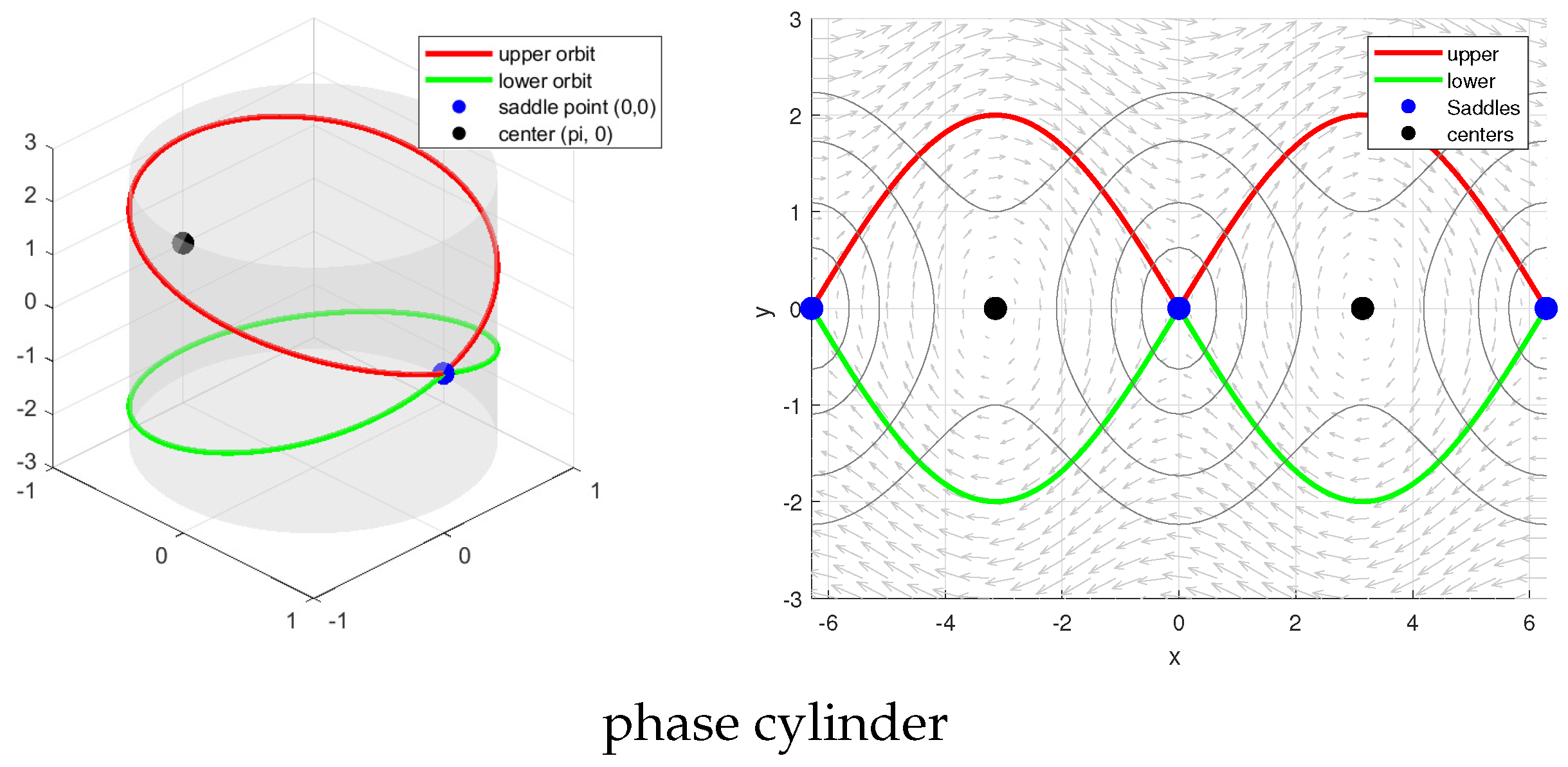
Note that in the plane $z=0$, the orbit is rather heteroclinic than homoclinic. On the other hand, if we consider a phase cylinder with a unit radius, then the orbit becomes real homoclinic. Both presentations can be seen in Figure 1.

The author’s research in [5] is based on the extended Andronov–Melnikov theory for determining the occurrence of potential chaos in the dynamical system under consideration through a detailed study of the Melnikov function of the form

$$\begin{array}{ccc}M\left(t_0\right)\hfill & =& {\displaystyle {\int }_{-\infty }^{\infty }}\left(f_1{g}_2-f_2{g}_1+{\displaystyle \frac{\partial H}{\partial z}}{g}_3\right)(q_0(t-t_0),t)\mathrm{d}t\hfill \\ \hfill & & -{\displaystyle \frac{\partial H}{\partial z}}\left(\gamma \left(z_0\right)\right){\displaystyle {\int }_{-\infty }^{\infty }}{g}_3(q_0(t-t_0),t)\mathrm{d}t\hfill \end{array}$$

(6)

or in a compact form,

$$\begin{array}{ccc}M\left(t_0\right)\hfill & =& {\displaystyle {\int }_{-\infty }^{\infty }}\left(\nabla H.G\right)(q_0\left(t\right),t+t_0)\mathrm{d}t\hfill \\ & & -{\displaystyle \frac{\partial H}{\partial z}}\left(\gamma \left(z_0\right)\right){\displaystyle {\int }_{-\infty }^{\infty }}{g}_3(q_0\left(t\right),t+t_0)\mathrm{d}t.\hfill \end{array}$$

For more details, see [5].

Research in this direction can be successfully continued.

As demonstrated in [12,13,14,15,16], the intricate dynamic behavior of third-order PLLs is extensively discussed.

PLLs are employed in cascaded or parallel connections in the majority of real-world applications [17], where synchronization between the PLLs is crucial to determining their performance.

Since the PLL is a highly nonlinear system with applications in high-frequency domains, the linear system theory is insufficient to fully comprehend its features.

However, nonlinear notions like stability, bifurcation, and Lyapunov exponents cannot adequately investigate the high nonlinear occurrence in PLL.

Fractional-order analysis has been shown in the literature to be very compatible with real-time systems.

The synchronization of real-time circuits such as PLL, when linked together in networks, has not been extensively studied (see, for example, [18], where the reader can find a rather thorough bibliography).

In this article, we investigate the dynamics of modified third-order Phase-Locked Loops (PLLs).

Our goal here is to investigate the effect of the new factor ${\displaystyle \sum _{j=1}^N}{a}_j\sin \left(j\omega t\right)$ on the dynamics of the new model.

Using perturbation techniques based on Andronov–Melnikov concepts, we demonstrate that horseshoe chaos exists in three-dimensional nonautonomous systems.

Several simulations are carried out.

We also look at a generalization based on probability distributions.

We will consider a numerical example of the possible application of the Melnikov function in the modeling of a radiation Melnikov antenna diagram.

2. The New Model

Here, we define the following new modification of the (PLL) model (1):

$$\left\{\begin{array}{ccc}{\displaystyle \frac{\mathrm{d}x}{\mathrm{d}t}}\hfill & =& y-kb\sin \left(x\right)\hfill \\ {\displaystyle \frac{\mathrm{d}y}{\mathrm{d}t}}\hfill & =& \sin \left(x\right)-z\hfill \\ {\displaystyle \frac{\mathrm{d}z}{\mathrm{d}t}}\hfill & =& k\left(\sin \left(x\right)+{\displaystyle \sum _{i=1}^N}{a}_i\sin \left(i\omega t\right)\right),\hfill \end{array}\right.$$

(7)

where $a_j\ge 0;j=1,2,\dots ,N$ and the loop gain coefficient k in the modified model is of the order of $O\left(ϵ\right)$.

We will make it clear that the suggested model is theoretical and that experts in this field of study have an opinion.

Dynamics of the Modified Model: Melnikov Approach

We prove the existence of horseshoe chaos in the three-dimensional nonautonomous systems using the perturbation methods based on the ideas of Andronov–Melnikov.

Theorem 1.

(a) The Melnikov function corresponding to model (7) is of the following form:

$$M\left(t_0\right)={\displaystyle \frac{8b}{3}}-8\mp 2{\displaystyle \sum _{i=1}^N}{\displaystyle \frac{\pi a_i}{i\omega }}cos\left(i\omega t_0\right)\mathrm{sech}\left({\displaystyle \frac{i\pi \omega }{2}}\right).$$

(8)

(b) If the parameters $b,\omega$, and $a_i,i=1,2,\dots ,N$ satisfy the following inequality,

$$\left|{\displaystyle \frac{\frac{8b}{3}-8}{2{\displaystyle \sum _{i=1}^N}\frac{\pi a_i}{i\omega }\mathrm{sech}\left(\frac{i\pi \omega }{2}\right)}}\right|<1$$

(9)

then transverse homoclinic orbits will exist.

Proof. 

(a) For the Melnikov function, we have

$$\begin{array}{ccc}M\left(t_0\right)\hfill & =& {\displaystyle {\int }_{-\infty }^{\infty }}\left((\sin \left(x_h\right)-z_h)b\sin \left(x_h\right)+x_h\left(\sin \left(x_h\right)+{\displaystyle \sum _{i=1}^N}{a}_i\sin \left(i\omega (t+t_0)\right)\right)\right)\mathrm{d}t\hfill \\ & & -0{\displaystyle {\int }_{-\infty }^{\infty }}\left(\sin \left(x_h\right)+{\displaystyle \sum _{i=1}^N}{a}_i\sin \left(i\omega (t+t_0)\right)\right)\mathrm{d}t\hfill \\ & =& {\displaystyle {\int }_{-\infty }^{\infty }}\left(b{\sin }^2\left(x_h\right)+x_h\sin \left(x_h\right)+x_h{\displaystyle \sum _{i=1}^N}{a}_i\sin \left(i\omega (t+t_0)\right)\right)\mathrm{d}t\hfill \\ & =& {\displaystyle {\int }_{-\infty }^{\infty }}\left\{\begin{array}{c}b{\sin }^2(\pm 2\mathrm{arcos}\left(\tanh \left(t\right)\right))\pm 2\mathrm{arcos}\left(\tanh \left(t\right)\right)\sin (\pm 2\mathrm{arcos}\left(\tanh \left(t\right)\right))\hfill \\ \pm 2\mathrm{arcos}\left(\tanh \left(t\right)\right){\displaystyle \sum _{i=1}^N}{a}_i\sin \left(i\omega (t+t_0)\right)\hfill \end{array}\right\}\mathrm{d}t\hfill \\ & =& {\displaystyle \frac{8b}{3}}-8\pm 2{\displaystyle {\int }_{-\infty }^{\infty }}\left(\mathrm{arcos}\left(\tanh \left(t\right)\right){\displaystyle \sum _{i=1}^N}{a}_i\sin \left(i\omega (t+t_0)\right)\right)\mathrm{d}t={\displaystyle \frac{8b}{3}}-8\pm 2I^N.\hfill \end{array}$$

Using the equality

$$\sin \left(i\omega (t+t_0)\right)=\sin \left(i\omega t\right)cos\left(i\omega t_0\right)+cos\left(i\omega t\right)\sin \left(i\omega t_0\right)$$

we obtain

$$M\left(t_0\right)={\displaystyle \frac{8b}{3}}-8\pm 2I^N={\displaystyle \frac{8b}{3}}-8\pm 2(I_1^N+I_2^N),$$

where

$$I_1^N={\displaystyle {\int }_{-\infty }^{\infty }}\mathrm{arcos}\left(\tanh \left(t\right)\right){\displaystyle {\displaystyle \sum _{i=1}^N}}{a}_i\sin \left(i\omega t\right)cos\left(i\omega t_0\right)\mathrm{d}t,$$

$$I_2^N={\displaystyle {\int }_{-\infty }^{\infty }}\mathrm{arcos}\left(\tanh \left(t\right)\right){\displaystyle {\displaystyle \sum _{i=1}^N}}{a}_{i}cos\left(i\omega t\right)\sin \left(i\omega t_0\right)\mathrm{d}t.$$

Let $N=1$. Then

$$I_1^1=a_{1}cos\left(\omega t_0\right){\displaystyle {\int }_{-\infty }^{\infty }}\mathrm{arcos}\left(\tanh \left(t\right)\right)\sin \left(\omega t\right)\mathrm{d}t.$$

Applying the Fourier transform to the function ${\displaystyle \frac{\mathrm{d}\left(\arccos \right(\tanh \left(t\right)\left)\right)}{\mathrm{d}t}}$ and taking into account that ${\displaystyle \frac{\mathrm{d}\left(\arccos \right(\tanh \left(t\right)\left)\right)}{\mathrm{d}t}}=-\mathrm{sech}\left(t\right)$, we can easily calculate that

$$I_1^1=-{\displaystyle \frac{\pi a_1}{\omega }}cos\left(\omega t_0\right)\mathrm{sech}\left({\displaystyle \frac{\pi \omega }{2}}\right).$$

For every N, the representation is valid

$$I_1^N=-{\displaystyle \sum _{i=1}^N}{\displaystyle \frac{\pi a_i}{i\omega }}cos\left(i\omega t_0\right)\mathrm{sech}\left({\displaystyle \frac{i\pi \omega }{2}}\right).$$

It is easy to calculate that the integral $I_2^N=0$ for every N.

Finally, for the Melnikov function, $M\left(t_0\right)$ we obtain

$$M\left(t_0\right)={\displaystyle \frac{8b}{3}}-8\mp 2{\displaystyle \sum _{i=1}^N}{\displaystyle \frac{\pi a_i}{i\omega }}cos\left(i\omega t_0\right)\mathrm{sech}\left({\displaystyle \frac{i\pi \omega }{2}}\right).$$

(b) Inequality (9) follows immediately from representation (8).

This proves the theorem. □

Remark 1.

We will explicitly note that from (8), in the special case $N=1$, we obtain the well-known result of Chu and Chou [5] obtained for the model (1):

If the parameters $b,\omega ,k$ satisfy the following inequality

$$\left|{\displaystyle \frac{(8b/3-8)\cosh (\omega \pi /2)}{2k\pi /\omega }}\right|<1$$

then the transverse homoclinic orbits will exist.

Remark 2.

Let $J_N$ denote the integral

$$J_N={\displaystyle {\int }_{-\infty }^{\infty }}\mathrm{arcos}\left(\tanh \left(t\right)\right)\sin \left(N\omega t\right)\mathrm{d}t.$$

In a number of cases, for studying the dynamics of models of the class of the proposed modification in this article, the following recursion relation may be useful:

$${\displaystyle \frac{1}{(N+1)J_{N+1}}}-2\cosh \left({\displaystyle \frac{\pi \omega }{2}}\right){\displaystyle \frac{1}{N{J}_N}}+{\displaystyle \frac{1}{(N-1)J_{N-1}}}=0.$$

Remark 3.

Suppose that ${\overline{a}}_i={\displaystyle \frac{a_i}{A}}$ for

$$A={\displaystyle \sum _{i=1}^N}{\displaystyle \frac{\pi a_i}{i\omega }}\mathrm{sech}\left({\displaystyle \frac{i\pi \omega }{2}}\right).$$

(10)

Note that $A>0$. Thus Melnikov function (8) can be rewritten as

$$M\left(t_0\right)={\displaystyle \frac{8b}{3}}-8\mp 2{\displaystyle A{\displaystyle \sum _{i=1}^N}}{a}_{i}cos\left(i\omega t_0\right).$$

(11)

The cos-trigonometric polynomial in (11) is a periodic function with a larger value achieved at zero, $P_{max}={\displaystyle A{\displaystyle \sum _{i=1}^N}}{a}_i>0$. Note that the lower value $P_{min}$ is negative. We may conclude that if $b=3$, then the Melnikov function has simple zeroes. On the other hand, if $b\ne 3$, then there exists a critical value $\overline{A}$ for A such that the Melnikov function (a.) has not roots for $A<\overline{A}$, (b.) has only multiple roots when $A=\overline{A}$, and (c.) has simple roots when $A>\overline{A}$.

It is known that chaos arises in the differential model under consideration if $M\left(t_0\right)=0$ and ${\displaystyle \frac{\mathrm{d}M\left(t_0\right)}{\mathrm{d}{t}_0}}\ne 0$ for some $t_0$ and some sets of parameters.

We generate the Melnikov equation $M\left(t_0\right)=0$ and analyze all of its zeroes using a specially designed software program.

Some numerical methods for solving the polynomial equation can be found in [19].

This gives the researcher the chance to accurately comprehend, articulate, and analyze all of the zeroes of the classical Melnikov criterion for the potential emergence of chaos in the dynamical system.

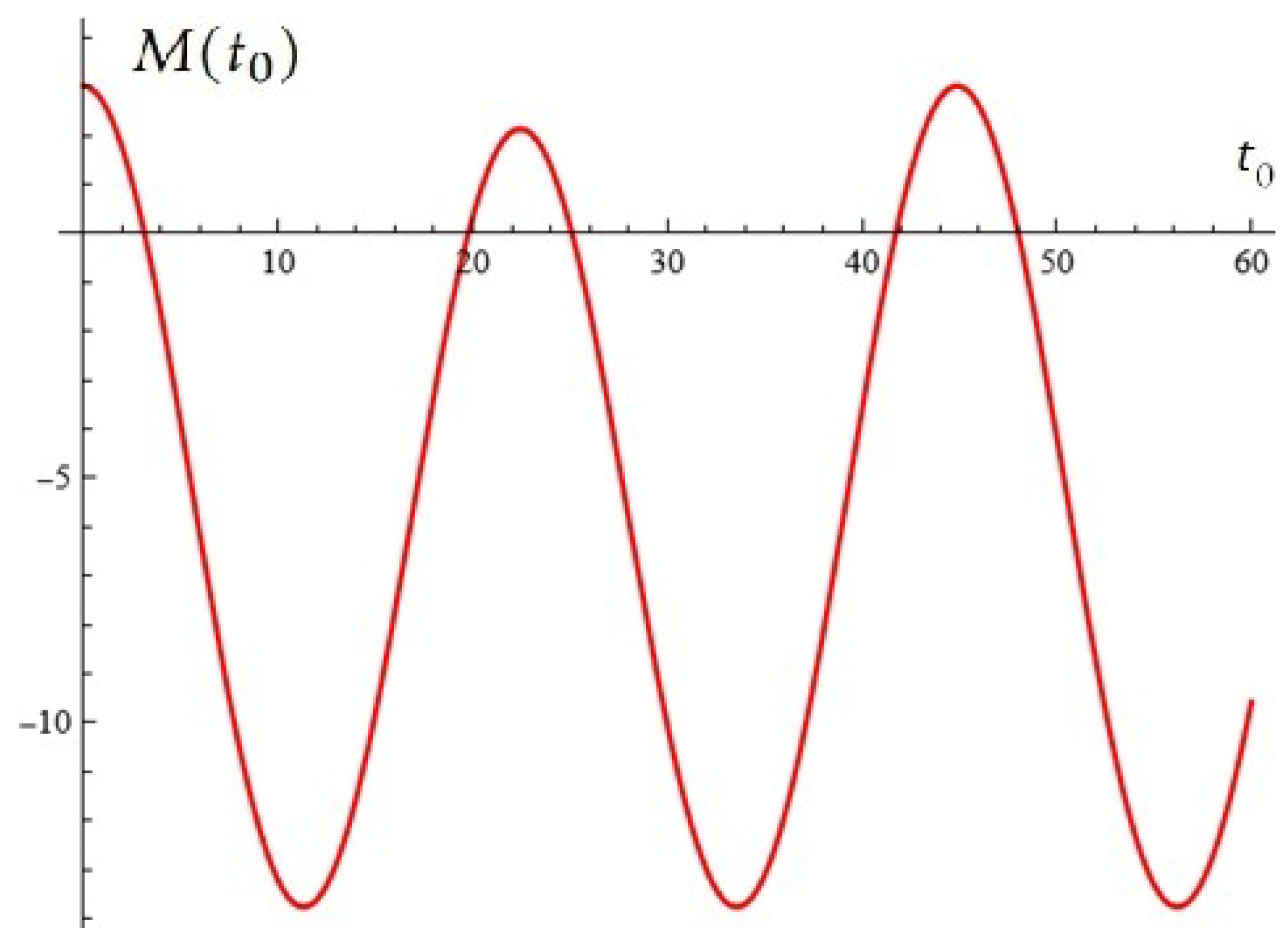
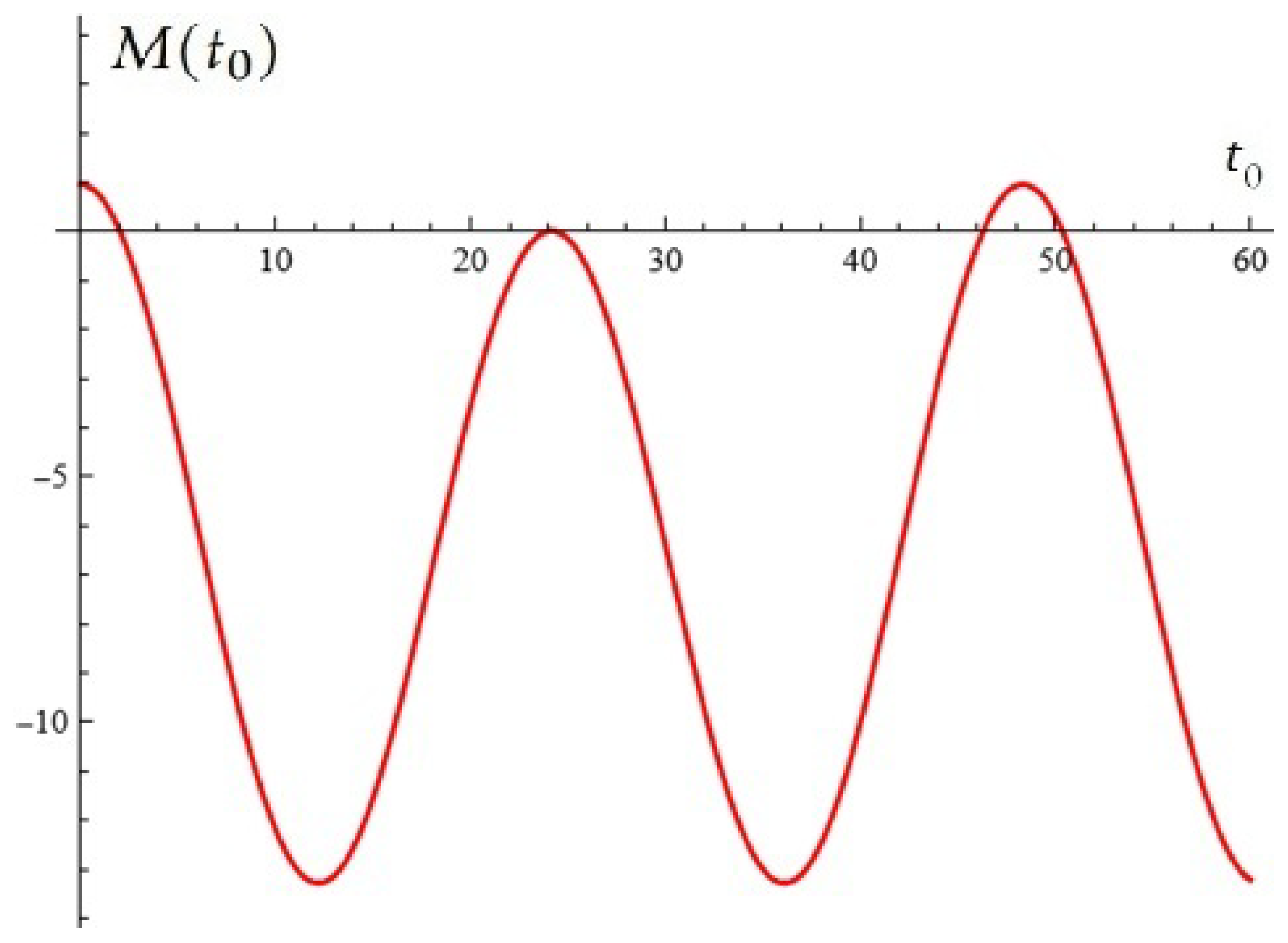
Numerical Example 1. Figure 2 shows the Melnikov function $M\left(t_0\right)$ for a given $N=2$, $\omega =0.14$, $b=0.9$, $a_1=0.01$, $a_2=0.4$.

The roots (in the confidence interval) appear to be with multiplicity one.

For small enough values of k, the differential system displays chaotic behavior in the sense of Smale–Birkhoff [20,21,22] because of the stable and unstable manifolds cross-transversally.

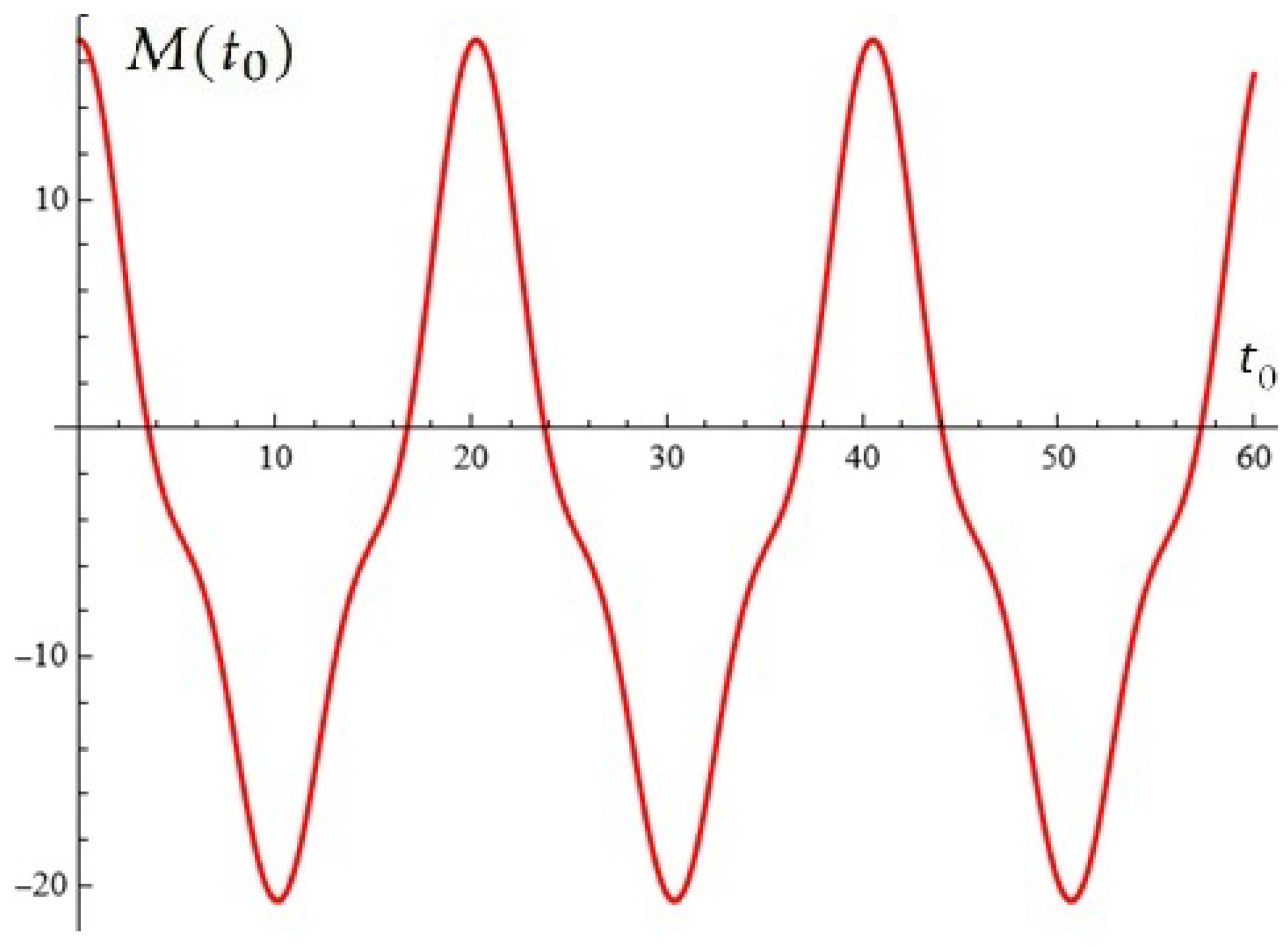
Numerical Example 2. Figure 3 shows the Melnikov function $M\left(t_0\right)$ for a given $N=2$, $\omega =0.13$, $b=0.6$, $a_1=0.01$, $a_2=0.309$.

There is tangent contact between the stable and unstable manifolds since $M\left(t_0\right)$ (in the confidence interval) has single roots and multiple roots $t_0\approx 24.6$ of multiplicity two.

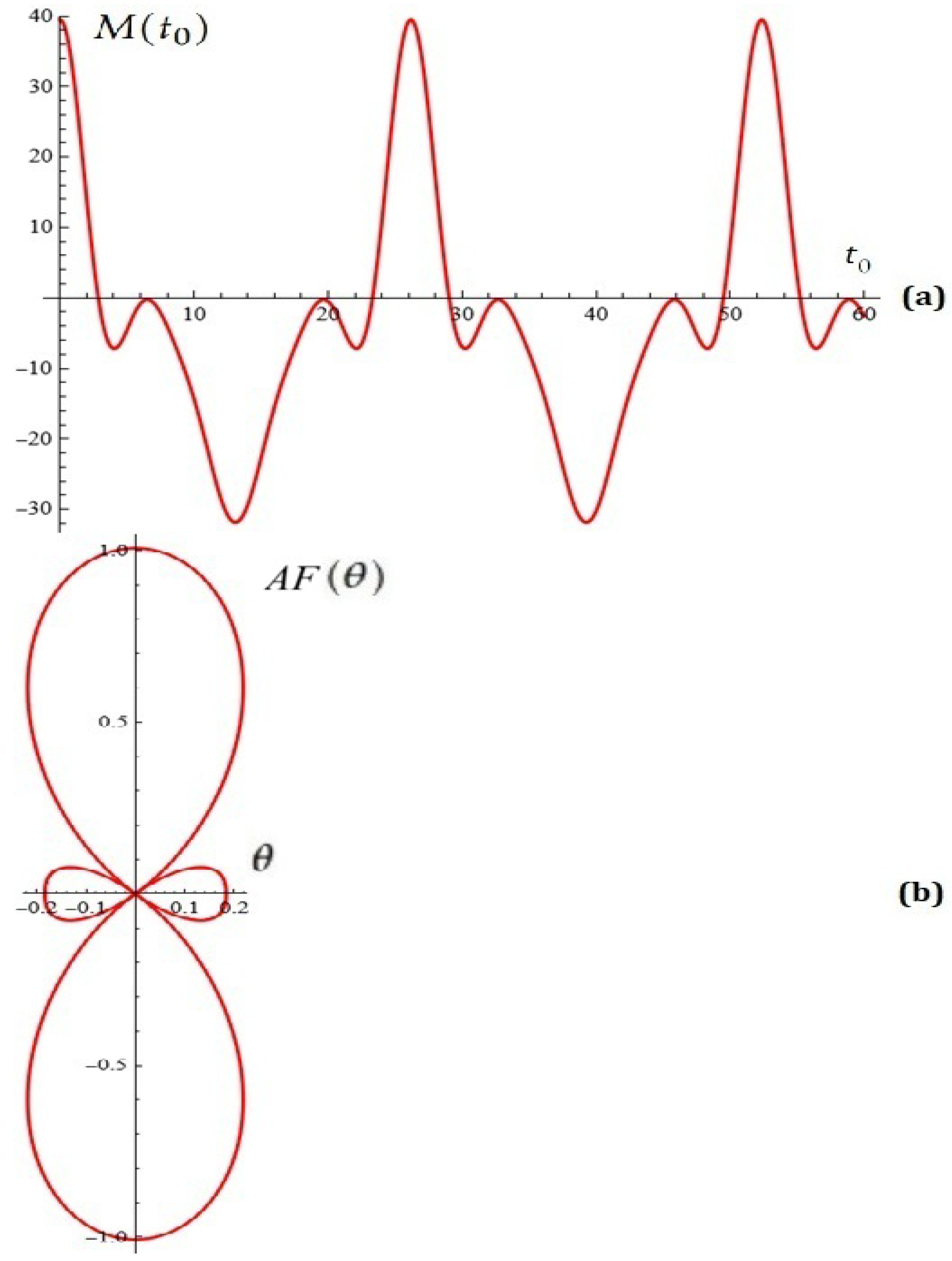
Numerical Example 3. Figure 4 shows the Melnikov function $M\left(t_0\right)$ for a given $N=3$, $\omega =0.31$, $b=1.8$, $a_1=0.86$, $a_2=0.2$, $a_3=1.1$.

The roots (in the confidence interval) appear to be with multiplicity one.

3. Simulations

Example 1.

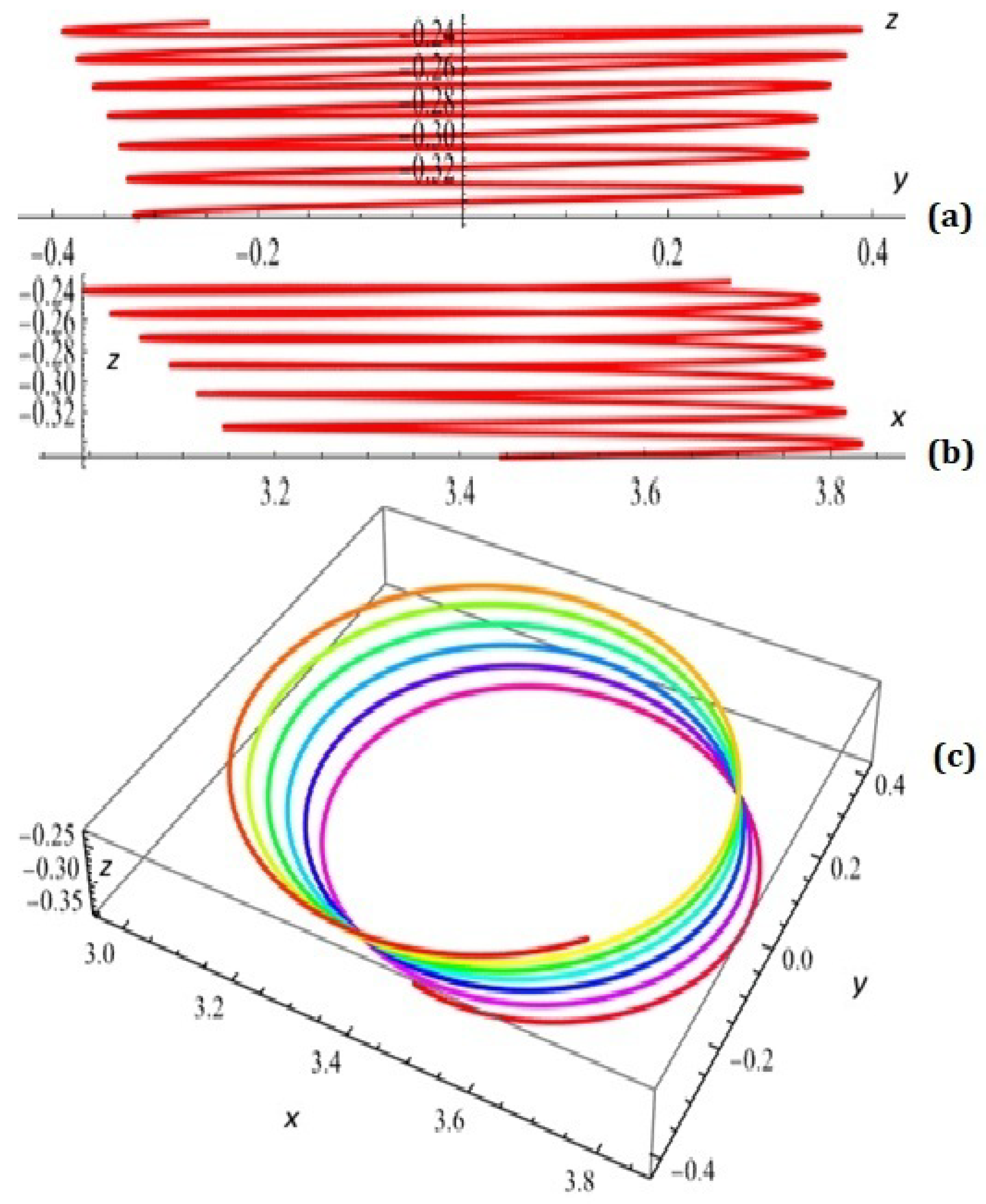
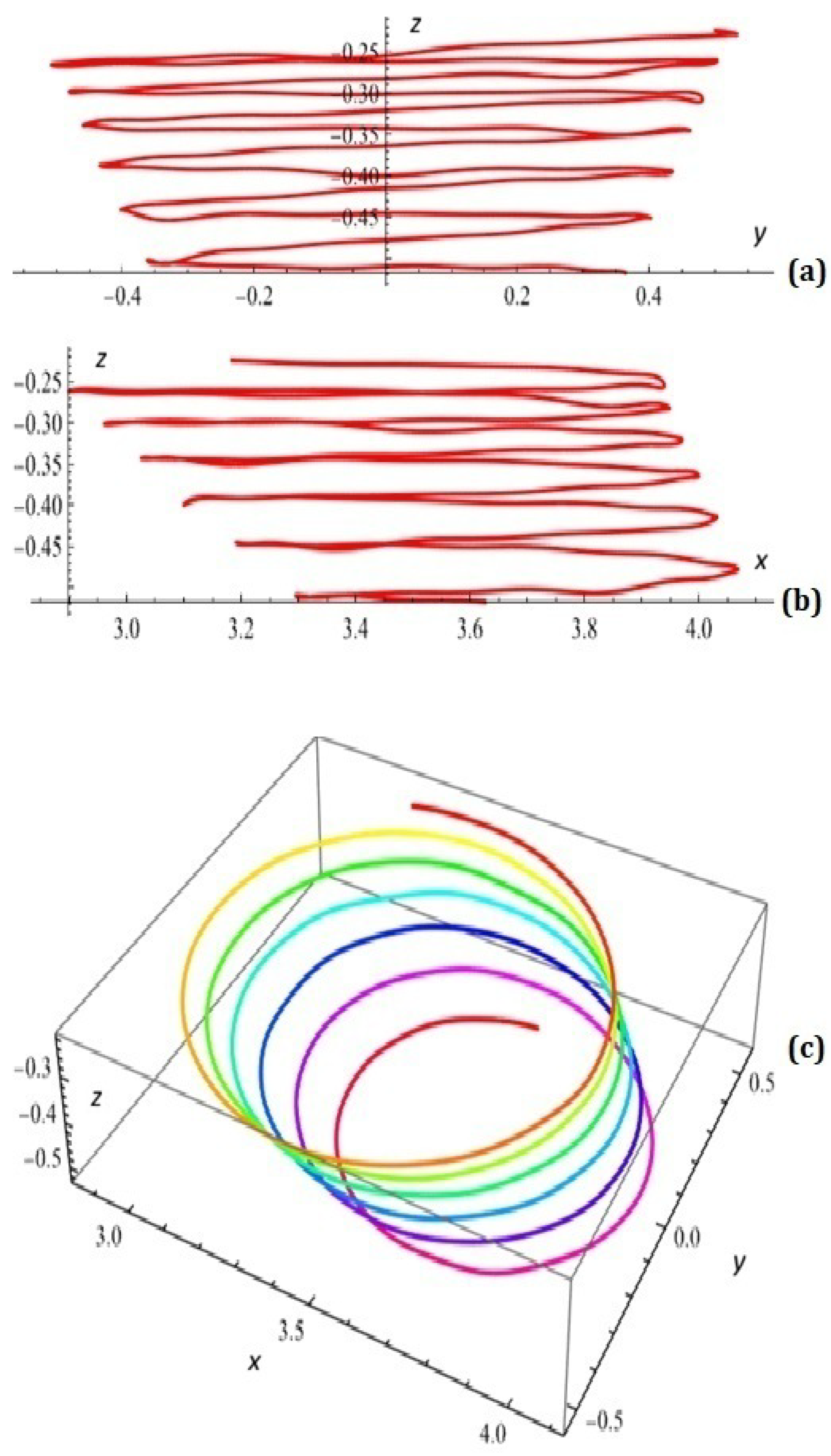
Let $N=1$, $b=0.1$; $k=0.01$; $\omega =1.1$; $a_1=0.15$.

The simulation on system (7) with initial approximation $x_0=3.8; y_0=0.04; z_0=-0.3$ is depicted on Figure 5.

Example 2.

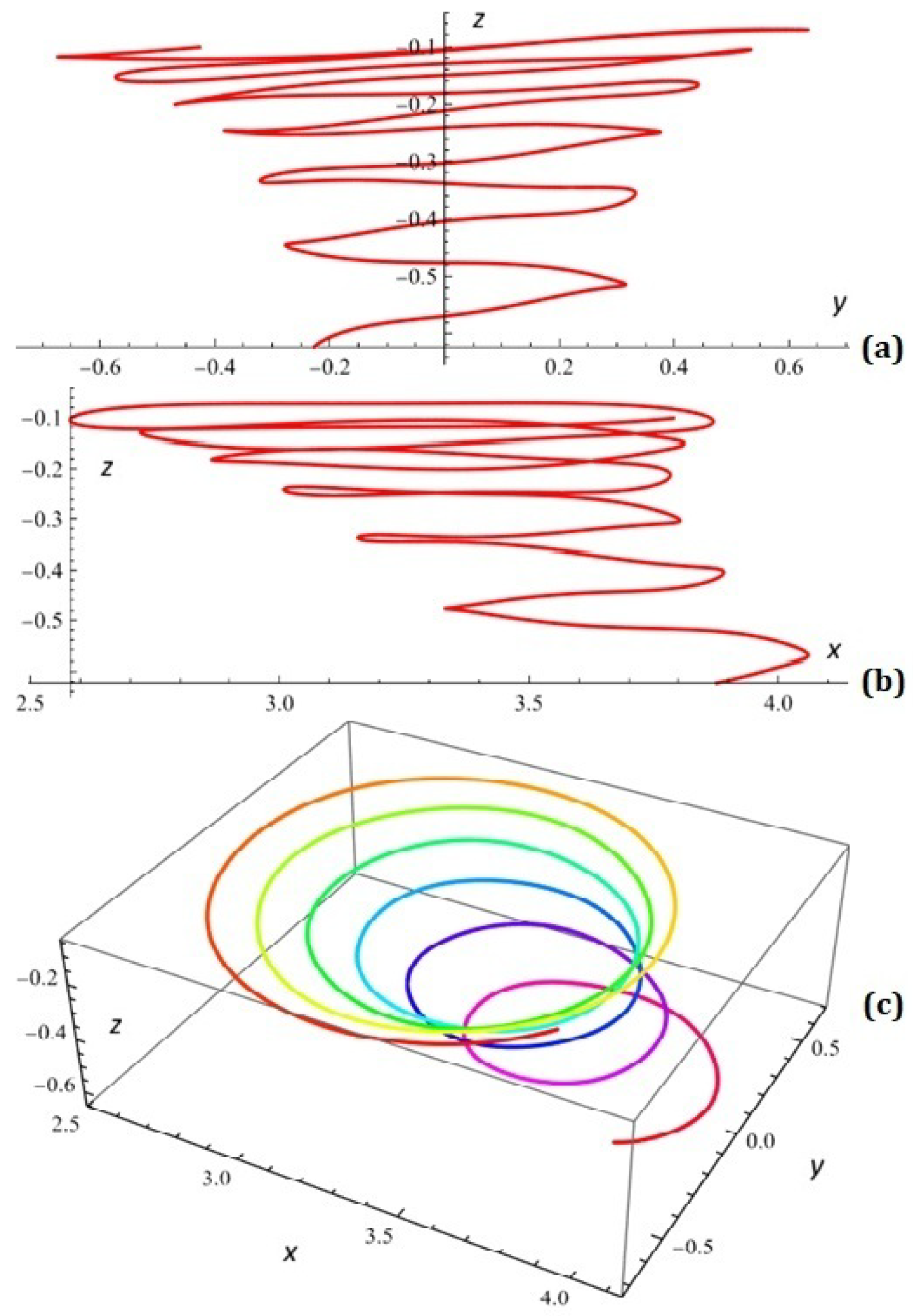
Let $N=3$, $b=0.1$; $k=0.05$; $\omega =1.1$; $a_1=0.15$; $a_2=0.05$; $a_3=0.3$.

The simulation on system (7) with initial approximation $x_0=3.8; y_0=0.04; z_0=-0.3$ is depicted on Figure 6.

Example 3.

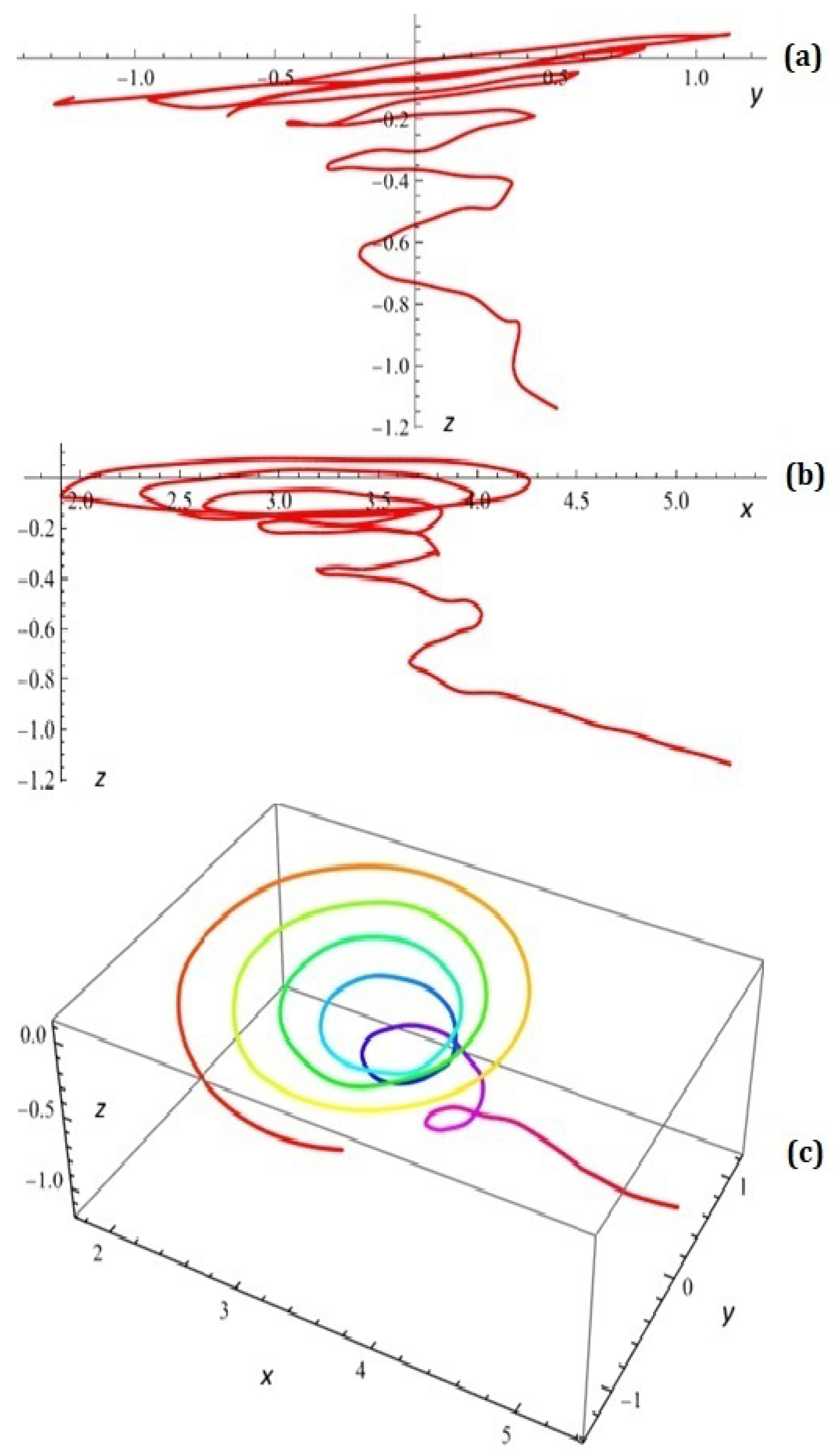
Let $N=6$, $b=0.1$; $k=0.1$; $\omega =1.1$; $a_1=0.15$; $a_2=0.05$; $a_3=0.3$; $a_4=0.2$; $a_5=0.1$; $a_6=0.25$.

The simulation on system (7) with initial approximation $x_0=3.8; y_0=0.04; z_0=-0.3$ is depicted on Figure 7.

Challenges for Learners

In addition to encouraging our PhD students to think about the triangle of enigmatics, creativity, and acmeology, we offer an effective study method that prioritizes learning.

Following the delivery of curricular modules, we will assign the following self-learning task.

Task 1 (self-learning). Examine how model (7) behaves with constant values of $N=9$, $b=0.1$, $\omega =1.1$, and $x_0=3.1; y_0=-0.015; z_0=-0.4$:

(a)

The dynamics shown in Figure 8 are achieved for what values of the parameters k, $a_i;i=1,2,\dots ,8$?

Answer: The approximate values $k=0.02$; $a_1=0.15$; $a_2=0.05$; $a_3=0.3$; $a_4=0.2$; $a_5=0.1$; $a_6=0.2$; $a_7=0.4$; $a_8=0.1$; $a_9=0.5$ should be obtained if the problem is successfully solved.

(b)

Make the appropriate deductions.

It would be helpful if readers shared their experiences with the methodological issues with teaching this particular subject that we have brought up.

The next task assumes that our PhD students are familiar with the theoretical analysis of Lyapunov exponents (Benettin algorithm, Gram–Schmidt orthonormalization over long time horizon, etc.) For more details, see [23,24,25,26,27,28,29].

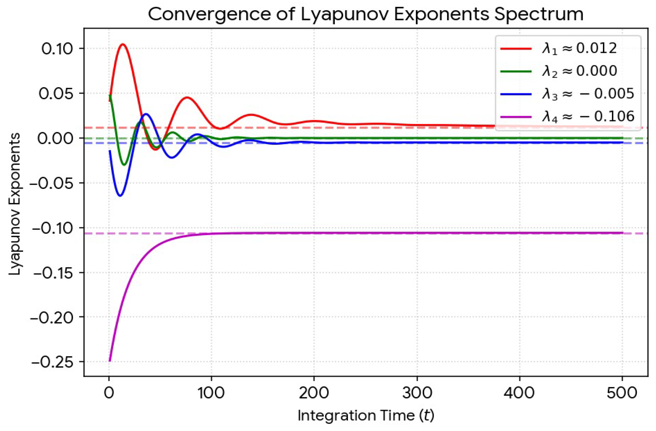
Task 2. (Self-learning with increased difficulty). Let us look again at model (7) with the data from Example 3. To compute Lyapunov exponents, we treat the system as a 4D autonomous system by introducing a phase variable $\varphi =\omega t$, where ${\displaystyle \frac{\mathrm{d}\varphi }{\mathrm{d}t}}=\omega$

$$\left\{\begin{array}{ccc}{\displaystyle \frac{\mathrm{d}x}{\mathrm{d}t}}\hfill & =& y-0.01\sin \left(x\right)\hfill \\ {\displaystyle \frac{\mathrm{d}y}{\mathrm{d}t}}\hfill & =& \sin \left(x\right)-z\hfill \\ {\displaystyle \frac{\mathrm{d}z}{\mathrm{d}t}}\hfill & =& 0.1\left(\sin \left(x\right)+{\displaystyle \sum _{i=1}^N}{a}_i\sin \left(i\varphi \right)\right)\hfill \\ {\displaystyle \frac{\mathrm{d}\varphi }{\mathrm{d}t}}\hfill & =& 1.1.\hfill \end{array}\right.$$

Numerical simulation using standard ODE Solver (like in MATLAB R2024b or in Python 3.14.5) combined with QR decomposition for orthogonalization yields the following spectrum: ${\lambda }_1\approx 0.012$ (largest Lyapunov exponent); ${\lambda }_2\approx 0.0000$ (neutral exponent); ${\lambda }_3\approx -0.005$ (negative exponent); ${\lambda }_4\approx -0.1060$ (extremely negative exponent). Because the maximum Lyapunow exponent ${\lambda }_1$ is positive, the system exhibits chaotic behavior. The sum of exponents is negative $\left(\sum {\lambda }_i\approx -0.099\right)$, confirming the system is dissipative and the dynamics converge to a strange attractor with a fractional Kaplan–Yorke dimension [30,31,32] $D_{KY}\approx 3.066$.

(a)

Illustrate Lyapunov Exponents’ Spectrum Numerical Convergence;

(b)

Draw the corresponding conclusions;

Answer: The image depicted in Figure 9 should be obtained if the problem is appropriately handled.

Interpretation. At the beginning of the simulation, the exponents vary strongly due to transient processes (transient chaos). After enough time, the lines smooth out and tend toward stable values. The positive value of the highest line is visual evidence of chaos!

(c)

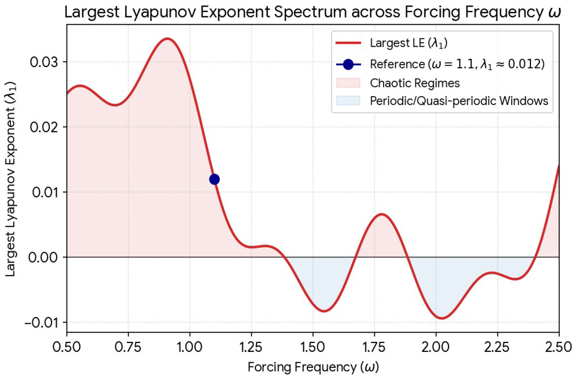
Try to illustrate the change in the largest Lyapunov exponent when varying $\omega$ in the interval $(0.5,2.5)$;

Answer: A sample visualization illustrating the influence of the omega frequency on the stability of the system is shown in Figure 10. The plot illustrates how the largest Lyapunov exponent $\left({\lambda }_1\right)$ changes as the driving frequency $\omega$ varies from 0.5 to 2.5. The curve clearly captures the transition through the weakly chaotic regime at $\omega =1.1$ $({\lambda }_1\approx 0.012)$, along with periodic windows and peak resonance zones.

(d)

Use the capabilities provided by existing scientific computing platforms (with paid or free access) and Artificial Intelligence services to solve the above task. Perform a thorough analysis in cases where the results provided to you differ from the results you obtained.

4. Generalization Based on Probability Distributions

We shall now modify model (7). Let $b_j={\displaystyle \frac{a_j}{j}}$, $B={\sum }_{v=1}^N{b}_j$ and $p_j={\displaystyle \frac{b_j}{B}}$ for $j=1,2,\dots ,N$. Let $\xi$ be a random variable on the sample space $\left\{1,2,\dots ,N\right\}$ with probabilities $\mathbb{P}\left(\xi =j\right)=p_j$. Note that $p_j\ge 0$ and ${\sum }_{j=1}^N{p}_j=1$. Thus, we can rewrite model (7) as

$$\begin{array}{cc}\hfill {\displaystyle \frac{\mathrm{d}x}{\mathrm{d}t}}& =y-kb\sin \left(x\right)\hfill \\ \hfill {\displaystyle \frac{\mathrm{d}y}{\mathrm{d}t}}& =\sin \left(x\right)-z\hfill \\ \hfill {\displaystyle \frac{\mathrm{d}z}{\mathrm{d}t}}& =k\left(\sin \left(x\right)+{\displaystyle \sum _{j=1}^N}{a}_j\sin \left(\omega t\right)\right)\hfill \\ \hfill & =k\left(\sin \left(x\right)+B{\displaystyle \sum _{j=1}^N}{p}_{j}j\sin \left(j\omega t\right)\right).\hfill \end{array}$$

(12)

Using the complex presentation of the sin-function

$$\sin \left(t\right)={\displaystyle \frac{e^{it}-e^{-it}}{2i}},$$

(13)

we transform the z-component of (12) into

$$\begin{array}{cc}\hfill {\displaystyle \frac{\mathrm{d}z}{\mathrm{d}t}}& =k\left(\sin \left(x\right)+B\mathbb{E}\left[\xi \sin \left(\xi \omega t\right)\right]\right)\hfill \\ \hfill & =k\left(\sin \left(x\right)+B\mathbb{E}\left[\xi {\displaystyle \frac{e^{i\xi \omega t}-e^{-i\xi \omega t}}{2i}}\right]\right)\hfill \\ \hfill & =k\left(\sin \left(x\right)+B{\displaystyle \frac{{\mathrm{\Psi }}^{\prime }\left(-\omega t\right)-{\mathrm{\Psi }}^{\prime }\left(\omega t\right)}{2}}\right),\hfill \end{array}$$

(14)

where the characteristic function of the random variable $\xi$ is represented by $\mathrm{\Psi }\left(·\right)$. We can abandon the restriction that this random variable is defined on the integers less than N considering an arbitrary domain D. Following the proof of Theorem 1, we obtain the following for the Melnikov integral (8):

$$\begin{array}{cc}\hfill M\left(t_0\right)& ={\displaystyle \frac{8b}{3}}-8\mp 2{\displaystyle \frac{\pi B}{\omega }}{\displaystyle \underset{-\infty }{\overset{\infty }{\int }}}\left(cos\left(v\omega t_0\right)\mathrm{sech}\left({\displaystyle \frac{v\pi \omega }{2}}\right)\right)p\left(\mathrm{d}v\right)\hfill \\ \hfill & ={\displaystyle \frac{8b}{3}}-8\mp {\displaystyle \frac{B}{\omega }}{\displaystyle \underset{-\infty }{\overset{\infty }{\int }}}\mathrm{\Psi }\left(u\right)\left({\displaystyle \underset{-\infty }{\overset{\infty }{\int }}}{e}^{-iuv}cos\left(v\omega t_0\right)\mathrm{sech}\left({\displaystyle \frac{v\pi \omega }{2}}\right)\mathrm{d}v\right)\mathrm{d}u\hfill \\ \hfill & ={\displaystyle \frac{8b}{3}}-8\mp {\displaystyle \frac{B}{2\omega }}{\displaystyle \underset{-\infty }{\overset{\infty }{\int }}}\mathrm{\Psi }\left(u\right)\left({\displaystyle \underset{-\infty }{\overset{\infty }{\int }}}{e}^{-iuv}\left(e^{iv\omega t_0}+e^{-iv\omega t_0}\right)\mathrm{sech}\left({\displaystyle \frac{v\pi \omega }{2}}\right)\mathrm{d}v\right)\mathrm{d}u.\hfill \end{array}$$

(15)

Having in mind that the $\mathrm{sech}$ is a self-Fourier function, we obtain

$$\begin{array}{cc}\hfill M\left(t_0\right)& ={\displaystyle \frac{8b}{3}}-8\mp {\displaystyle \frac{B}{{\omega }^2}}{\displaystyle \underset{-\infty }{\overset{\infty }{\int }}}\mathrm{\Psi }\left(u\right)\left(\mathrm{sech}\left({\displaystyle \frac{u+\omega t_0}{\omega }}\right)+\mathrm{sech}\left({\displaystyle \frac{u-\omega t_0}{\omega }}\right)\right)\mathrm{d}u\hfill \\ \hfill & ={\displaystyle \frac{8b}{3}}-8\mp {\displaystyle \frac{B}{\omega }}{\displaystyle \underset{-\infty }{\overset{\infty }{\int }}}\mathrm{\Psi }\left(\omega v\right)\left(\mathrm{sech}\left(v+t_0\right)+\mathrm{sech}\left(v-t_0\right)\right)\mathrm{d}v.\hfill \end{array}$$

(16)

Considering that the real part of $\mathrm{\Psi }\left(·\right)$ is an even function, the imaginary part is odd, and $\mathrm{sech}\left(v+t_0\right)+\mathrm{sech}\left(v-t_0\right)$ is even, we rewrite the Melnikov integral as

$$M\left(t_0\right)={\displaystyle \frac{8b}{3}}-8\mp 2{\displaystyle \frac{B}{\omega }}{\displaystyle \underset{0}{\overset{\infty }{\int }}}\Re \mathrm{\Psi }\left(\omega v\right)\left(\mathrm{sech}\left(v+t_0\right)+\mathrm{sech}\left(v-t_0\right)\right)\mathrm{d}v.$$

(17)

We shall now provide an example based on a $\left(\mu ,{\sigma }^2\right)$-Gaussian distribution. Its characteristic function is

$${\mathrm{\Psi }}_{\xi }\left(x\right)=e^{i\mu x-{\displaystyle \frac{{\sigma }^2{x}^2}{2}}},$$

(18)

which leads to

$${\mathrm{\Psi }}_{\xi }\left(x\right)-{\mathrm{\Psi }}_{\xi }\left(-x\right)=-2e^{-{\displaystyle \frac{{\sigma }^2{x}^2}{2}}}\left(\mu \sin \left(\mu x\right)+{\sigma }^{2}xcos\left(\mu x\right)\right).$$

(19)

Thus, the model dynamics turn into

$$\begin{array}{cc}\hfill {\displaystyle \frac{\mathrm{d}x}{\mathrm{d}t}}& =y-kb\sin \left(x\right)\hfill \\ \hfill {\displaystyle \frac{\mathrm{d}y}{\mathrm{d}t}}& =\sin \left(x\right)-z\hfill \\ \hfill {\displaystyle \frac{\mathrm{d}z}{\mathrm{d}t}}& =k\left(\sin \left(x\right)+B{e}^{-{\displaystyle \frac{{\sigma }^2{\omega }^2{t}^2}{2}}}\left(\mu \sin \left(\mu \omega t\right)+{\sigma }^2\omega tcos\left(\mu \omega t\right)\right)\right)\hfill \end{array}$$

(20)

and its Melnikov integral is

$$M\left(t_0\right)={\displaystyle \frac{8b}{3}}-8\mp 2{\displaystyle \frac{B}{\omega }}{\displaystyle \underset{0}{\overset{\infty }{\int }}}{e}^{-{\displaystyle \frac{{\sigma }^2{\omega }^2{v}^2}{2}}}cos\left(\mu \omega v\right)\left(\mathrm{sech}\left(v+t_0\right)+\mathrm{sech}\left(v-t_0\right)\right)\mathrm{d}v.$$

(21)

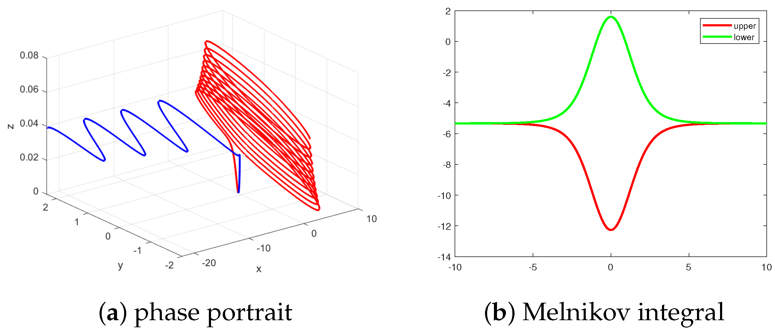
A particular example based on the following values is presented in Figure 11—$k=0.01$, $\omega =1.1$, $B=2.5$, $\mu =1$, $\sigma =1$, and $b=1$. Figure Figure 11a is for the phase portrait, whereas both Melnikov functions are depicted in Figure 11b. We can observe that one of them has simple roots whereas the other has no roots.

5. Concluding Remarks

1.

We have suggested and examined a version of the PLL model with numerous free parameters in this study, which might be of some use to experts in the field: Phase-Locked Loop Methods.

2.

The dynamic analysis conducted in the sense of Andronov–Melnikov can be used in studying other, modified models, both traditional and more recent, that have been published in the literature.

3.

Additionally, we include a few specific modules for examining the dynamics of the model under consideration (PLL).

4.

This will be a crucial component of a much broader web-based scientific computing application (see [33]).

5.

Other techniques related to the use of perturbation factors with many free parameters (see, for example, [34,35]) can be successfully applied to other interesting modifications of PLL models, jerk oscillators [36,37,38,39,40,41,42,43,44] and oscillator circuit models [45,46,47,48,49,50,51,52,53,54,55,56].

We envisage future research in the above-mentioned scientific areas.

6.

A potential use of the Melnikov functions (which correspond to distinct differential systems) in the modeling and synthesis of radiation antenna diagrams was covered in our earlier publications. We shall not discuss these matters here.

The article [35] contains enough information for the reader.

Only a few numerical examples of the potential applications of the Melnikov polynomial corresponding to the generalized differential model under consideration in this paper will be examined.

The hypothetical normalized antenna factor is defined as follows:

$$AF\left(\theta \right)={\displaystyle \frac{1}{D}}\left|M(Kcos\theta +k_1)\right|,$$

where d is the distance between emitters, $k_1$ is the phase difference, $\theta$ is the azimuth angle, and $K=kd;k={\displaystyle \frac{2\pi }{\lambda }};\lambda$ is the wave length.

Example 4.

For fixed $N=5$, $K=4.1$, $k_1=0$, $\omega =0.24$, $b=1.7$. $a_1=0.86$, $a_2=0.2$, $a_3=2.3$, $a_4=1.9$, $a_5=1.9$, the Melnikov function and Melnikov antenna factor are depicted in Figure 12.

In fact, experts in this field of study are seriously investigating this relatively new concept.

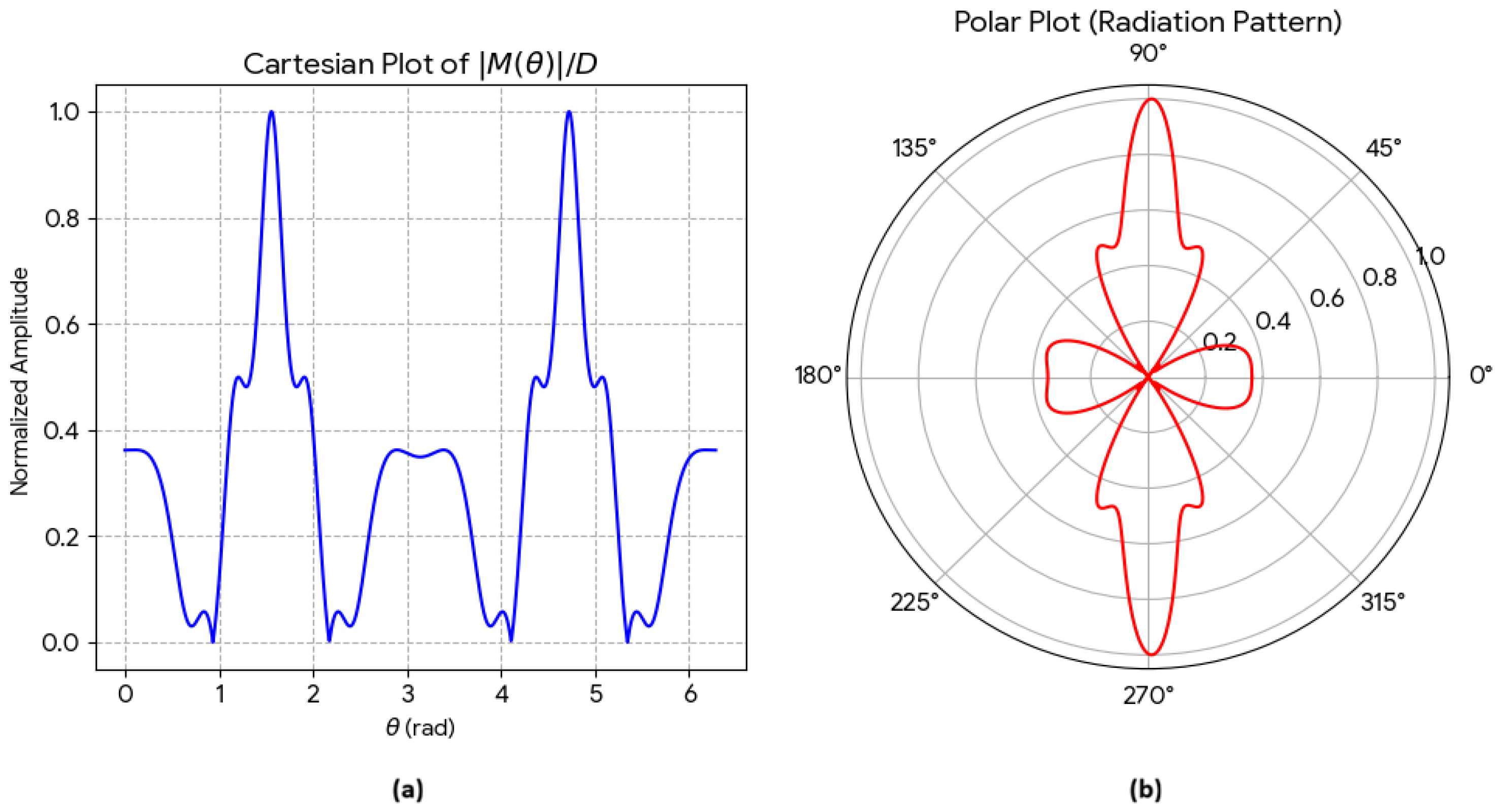
Task 3. (self-learning with increased difficulty). Let $N=11$, $\omega =0.2$, $b=1.4$, $a_1=0.3$, $a_2=0.05$, $a_3=0.1$, $a_4=0.091$, $a_5=0.81$, $a_6=0.07$, $a_7=0.06$; $a_8=0.05$; $a_9=0.04$; $a_{10}=0.3$; $a_{11}=0.01$. For $K=16$ and $k_1=-0.2$:

(a)

Generate antenna factor $AF\left(\theta \right)$;

(b)

Cartesian plot of $AF\left(\theta \right)$;

Answer.

If you solve the given problem correctly, you should obtain the images shown in Figure 13.

(c)

Try to minimize the level of side radiation with the new array data set;

(d)

Draw the corresponding conclusions.

We anticipate future research on the dynamic behavior of a high-order PPL using the extended high-dimensional Melnikov method following the ideas given in [57].

References

1. Viterbi, A.J. Principles of Coherent Communication; McGraw-Hill: New York, NY, USA, 1966. [Google Scholar]
2. Endo, T.; Chua, L.O. Chaos from phase-locked loop. IEEE Trans. Circuits Syst. 1988, 35, 987–1003. [Google Scholar] [CrossRef] [Scilit]
3. Endo, T.; Chua, L.O.; Narita, T. Chaos from phase-locked loops—Part II: High-dissipation case. IEEE Trans. Circuits Syst. 1989, 35, 255–263. [Google Scholar] [CrossRef]
4. Hsich, G.-C.; Huang, J.C. Phase-Locked Loop Techniques—A Survey. IEEE Trans. Ind. Electron. 1996, 43, 609–615. [Google Scholar]
5. Chu, Y.-H.; Chou, J.-H. Chaos from third-order Phase-Locked Loops with a slowly varying parameter. IEEE Trans. Circuits Syst. 1990, 37, 1104–1115. [Google Scholar] [CrossRef]
6. Melnikov, V. On the stability of the center for time periodic perturbations. Trans. Moskow Math. Soc. 1963, 12, 3–52. [Google Scholar]
7. Wiggins, S. Introduction to Applied Nonlinear Dynamical Systems and Chaos; Texts in Applied Mathematics; Springer: New York, NY, USA, 1990; Volume 2. [Google Scholar]
8. Guckenheimer, J.; Holmes, P.J. Nonlinear Oscillations, Dynamical Systems, and Bifurcations of Vector Fields; Applied Mathematical Sciences; Springer: New York, NY, USA, 1983; Volume 42. [Google Scholar]
9. Wiggins, S.; Shaw, S.W. Chaos and three-dimensional horseshoes in slowly varying oscillators. SIAM J. Appl. Mech. 1988, 55, 958–968. [Google Scholar] [CrossRef] [Scilit]
10. Thompson, J.M.T.; Stewart, H.B. Nonlinear Dynamics and Chaos; Wiley: New York, NY, USA, 1986. [Google Scholar]
11. Wiggins, S.; Holmes, P.J. Homoclinic orbits in slowly varying oscillators. SIAM J. Math. Anal. 1988, 19, 1254–1255. [Google Scholar] [CrossRef] [Scilit]
12. Piqueira, J.R.C. Using bifurcations in the determination of lock-in ranges for third-order phase-locked loops. Commun. Nonlinear Sci. Numer. Simul. 2009, 14, 2328–2335. [Google Scholar] [CrossRef] [Scilit]
13. Best, R.E. Phase-Locked Loops: Design, Simulation, and Applications; McGraw-Hill: New York, NY, USA, 2003. [Google Scholar]
14. Monteiro, L.H.A.; Favaretto, D.N.; Piqueira, J.R.C. Bifurcation analysis for third-order phase-locked loops. IEEE Signal Process. Lett. 2004, 11, 494–496. [Google Scholar] [CrossRef] [Scilit]
15. Harb, B.A.; Harb, A.M. Chaos and bifurcation in a third-order phase locked loop. Chaos Solitons Fractals 2004, 19, 667–672. [Google Scholar] [CrossRef] [Scilit]
16. Sarkar, B.C.; Chakraborty, S. Self-oscillations of a third order PLL in periodic and chaotic mode and its tracking in a slave PLL. Commun. Nonlinear Sci. Numer. Simul. 2014, 19, 738–749. [Google Scholar] [CrossRef] [Scilit]
17. Qananwah, Q.M.; Malkawi, S.R.; Harb, A. Chaos synchronisation of the third-order phase-locked loop. Int. J. Electron. 2008, 95, 799–803. [Google Scholar] [CrossRef] [Scilit]
18. Karthikeyan, A.; Rajagopal, K. Network Dynamics of a Fractional-Order Phase-Locked Loop with Infinite Coexisting Attractors. Complexity 2020, 2020, 7902474. [Google Scholar] [CrossRef] [Scilit]
19. Sendov, B.; Andreev, A.; Kjurkchiev, N. Numerical solution of polynomial equations. In Handbook of Numerical Analysis; Ciarlet, P., Lions, J., Eds.; Elsevier: Amsterdam, The Netherlands, 1994; Volume III, pp. 625–778. [Google Scholar]
20. Birkhoff, G.D. Nouvelles recherches sur les systèmes dynamiques. In Collected Mathematical Papers; American Mathematical Society: Providence, RI, USA, 1950; Volume 2, pp. 530–662. [Google Scholar]
21. Smale, S. Diffeomorphisms with many periodic points. In Differential and Combinatorial Topology; Princeton University Press: Princeton, NJ, USA, 1965; pp. 63–80. [Google Scholar]
22. Smale, S. Differentiable dynamical systems. Bull. Am. Math. Soc. 1967, 73, 747–817. [Google Scholar] [CrossRef] [Scilit]
23. Halanay, A. Applications of Liapunov Methods in Stability; Kluwer Academic Publishers: Dordrecht, The Netherlands, 1993. [Google Scholar]
24. Benettin, G.; Galgani, L.; Giorgilli, A.; Strelcyn, J.-M. Lyapunov Characteristic Exponents for smooth dynamical systems and for hamiltonian systems; a method for computing all of them. Part 1: Theory. Meccanica 1980, 15, 9–20. [Google Scholar] [CrossRef] [Scilit]
25. Rosier, L.; Bacciotti, A. Liapunov Functions and Stability in Control Theory; Springer: Berlin/Heidelberg, Germany, 2010. [Google Scholar]
26. Pikovsky, A.; Politi, A. Lyapunov Exponents: A Tool to Explore Complex Dynamics; Cambridge University Press: Cambridge, UK, 2016. [Google Scholar]
27. Stoer, J.; Bulirsch, R. Introduction to Numerical Analysis, 3rd ed.; Springer: Berlin/Heidelberg, Germany, 2002. [Google Scholar]
28. Pchelintsev, A.N. An Accurate Numerical Method and Algorithm for Constructing Solutions of Chaotic Systems. J. Appl. Nonlinear Dyn. 2020, 9, 207–221. [Google Scholar] [CrossRef] [Scilit]
29. Holmes, M.H. Introduction to Scientific Computing and Data Analysis, 2nd ed.; Springer: Berlin/Heidelberg, Germany, 2023. [Google Scholar]
30. Kaplan, J.L.; Yorke, J.A. Chaotic behavior of multidimensional difference equations. In Functional Differential Equations and the Approximation of Fixed Points; Springer: Berlin/Heidelberg, Germany, 1979; pp. 204–227. [Google Scholar]
31. Evans, D.J.; Cohen, E.G.D.; Searles, D.J.; Bonetto, F. Note on the Kaplan–Yorke dimension and linear transport coefficients. J. Stat. Phys. 2000, 101, 17–29. [Google Scholar] [CrossRef] [Scilit]
32. Bakri, T.; Verhulst, F. A Note on the Kaplan–Yorke Dimension. Int. J. Bifurc. Chaos 2025, 35, 2550133. [Google Scholar] [CrossRef] [Scilit]
33. Golev, A.; Terzieva, T.; Iliev, A.; Rahnev, A.; Kyurkchiev, N. Simulation on a Generalized Oscillator Model: Web-Based Application. C. R. Acad. Bulg. Sci. 2024, 77, 230–237. [Google Scholar] [CrossRef] [Scilit]
34. Kyurkchiev, N.; Zaevski, T.; Vasileva, M.; Kyurkchiev, V.; Iliev, A.; Rahnev, A. Dynamics of a Class of Extended Duffing–Van Der Pol Oscillators: Melnikov’s Approach, Simulations, Control over Oscillations. Mathematics 2025, 13, 2240. [Google Scholar] [CrossRef] [Scilit]
35. Kyurkchiev, N.; Zaevski, T.; Iliev, A. Investigations on the Chaos in the Generalized Double Sine-Gordon Planar System: Melnikov’s Approach and Applications to Generating Antenna Factors. Mathematics 2025, 13, 3700. [Google Scholar] [CrossRef] [Scilit]
36. Kamdoum Tamba, V.; Takougang Kingni, S.; Fautso Kuiate, G.; Bertrand Fotsin, H.; Kisito Talla, P. Coexistence of attractors in autonomous Van der Pol–Duffing jerk oscillator: Analysis, chaos control and synchronisation in its fractional-order form. Pramana J. Phys. 2018, 91, 12. [Google Scholar] [CrossRef] [Scilit]
37. Benitez, M.S.; Zuppa, L.A.; Guerra, R.J.R. Chaotification of the Van der Pol system using Jerk architecture. IEICE Trans. Fundam. 2006, E89-A, 375–378. [Google Scholar] [CrossRef] [Scilit]
38. Malasoma, J.M. What is the simplest dissipative chaotic jerk equation which is parity invariant? Phys. Lett. A 2000, 264, 383. [Google Scholar] [CrossRef] [Scilit]
39. Gottlieb, H.P.W. Question 38. What Is the Simplest Jerk Function That Gives Chaos. Am. J. Phys. 1996, 64, 525. [Google Scholar] [CrossRef] [Scilit]
40. Sprott, J.C. A new chaotic jerk circuit. IEEE Trans. Circuits Syst. II Express Briefs 2011, 58, 240–243. [Google Scholar] [CrossRef] [Scilit]
41. Sprott, J.C. Elegant Chaos: Algebraically Simple Chaotic Flows; World Scientific: Singapore, 2010. [Google Scholar]
42. Acho, L.; Rolon, J.; Benitez, S.A. Chaotic oscillator using the Van der Pol dynamic immersed into a jerk system. WSEAS Trans. Circuits Syst. 2004, 3, 198–199. [Google Scholar]
43. Louodop, P.; Kountchou, M.; Fotsin, H.B.; Bowong, S. Practical finite-time synchronization of jerk systems: Theory and experiment. Nonlinear Dyn. 2014, 78, 597–607. [Google Scholar] [CrossRef] [Scilit]
44. Kengne, J.; Njitacke, Z.T.; Fotsin, H.B. Dynamical analysis of a simple autonomous jerk system with multiple attractors. Nonlinear Dyn. 2016, 83, 751–765. [Google Scholar] [CrossRef] [Scilit]
45. Chua, L.O.; Kocarev, L.J.; Eckert, K.; Itoh, M. Experimental chaos synchronization in Chua’s circuit. Int. J. Bifurc. Chaos 1992, 2, 705–708. [Google Scholar] [CrossRef] [Scilit]
46. Madan, R.A. Chua’s Circuit: A Paradigm for Chaos; World Scientific: Singapore, 1993. [Google Scholar]
47. Murali, K.; Lakshmanan, M.; Chua, L.O. Bifurcation and chaos in the simplest dissipative non-autonomous circuit. Int. J. Bifurc. Chaos 1994, 4, 1511–1524. [Google Scholar] [CrossRef] [Scilit]
48. Elwakil, A.S.; Soliman, A.M. A family of Wien-type oscillators modified for chaos. Int. J. Circuit Theory Appl. 1997, 25, 561–579. [Google Scholar] [CrossRef] [Scilit]
49. Baptista, M.S.; Caldas, I.L. Phase-locking and bifurcations of the sinusoidally-driven double scroll circuit. Nonlinear Dyn. 1998, 17, 119–139. [Google Scholar] [CrossRef] [Scilit]
50. Maggio, G.M.; Feo, O.D.; Kennedy, M.P. Nonlinear analysis of the colpitts oscillator and applications to design. IEEE Trans. Circuits Syst. I 1999, 46, 1118–1130. [Google Scholar] [CrossRef] [Scilit]
51. Thamilmaran, K.; Lakshmanan, M.; Murali, K. Rich variety of bifurcations and chaos in a variant of Murali-Lakshmanan-Chua circuit. Int. J. Bifurc. Chaos 1994, 10, 1781–1785. [Google Scholar] [CrossRef] [Scilit]
52. Sprott, J.C. A new class of chaotic circuits. Phys. Lett. A 2000, 266, 19–23. [Google Scholar] [CrossRef] [Scilit]
53. Elwakil, A.S.; Kennedy, M.P. Construction of classes of circuit independent chaotic oscillators using passive-only nonlinear. IEEE Trans. Circuits Syst. I 2001, 48, 289–307. [Google Scholar] [CrossRef] [Scilit]
54. Ma, J.; Li, A.B.; Pu, Z.S.; Yang, L.J.; Wang, Y.Z. A time-varying hyperchaotic system and its realization in circuit. Nonlinear Dyn. 2010, 62, 535–541. [Google Scholar] [CrossRef] [Scilit]
55. Tchitnga, R.; Fotsin, H.B.; Nana, B.; Louodop-Fotso, P.H.; Woafo, P. Hartley’s oscillator: The simplest chaotic two-component circuit. Chaos Solitons Fractals 2012, 45, 306–313. [Google Scholar] [CrossRef] [Scilit]
56. Vincent, U.E.; Nana Nbendjo, B.R.; Ajayi, A.A.; Njah, A.N.; McClintock, P.V.E. Hyperchaos and Bifurcations in a Driven Van der Pol-Duffing Oscillator Circuit. Int. J. Dyn. Control 2014, 3, 363–370. [Google Scholar] [CrossRef] [Scilit]
57. Li, H.; Shen, Y.; Li, J.; Dong, J.; Hong, G. On the Melnikov method for fractional-order systems. Chaos Solitons Fractals 2024, 188, 115602. [Google Scholar] [CrossRef] [Scilit]
Figure 1. Homoclinic orbit.
Mathematics 14 02071 g001
Figure 2. The Melnikov function M ( t 0 ) (Numerical Example 1).
Mathematics 14 02071 g002
Figure 3. The Melnikov function M ( t 0 ) (Numerical Example 2).
Mathematics 14 02071 g003
Figure 4. The Melnikov function M ( t 0 ) (Numerical Example 3).
Mathematics 14 02071 g004
Figure 5. Phase portraits (a) on plane ( y , z ) ; (b) on plane ( x , z ) ; (c) on plane ( x , y , z ) (Example 1).
Mathematics 14 02071 g005
Figure 6. Phase portraits (a) on plane ( y , z ) ; (b) on plane ( x , z ) ; (c) on plane ( x , y , z ) (Example 2).
Mathematics 14 02071 g006
Figure 7. Phase portraits (a) on plane ( y , z ) ; (b) on plane ( x , z ) ; (c) on plane ( x , y , z ) (Example 3).
Mathematics 14 02071 g007
Figure 8. Phase portraits (a) on plane ( y , z ) ; (b) on plane ( x , z ) ; (c) on plane ( x , y , z ) (Task 1).
Mathematics 14 02071 g008
Figure 9. Lyapunov Exponents Spectrum Numerical Convergence (Task 2).
Mathematics 14 02071 g009
Figure 10. Influence of the omega frequency on the stability of the system (Task 2).
Mathematics 14 02071 g010
Figure 11. Example based on the Gaussian distribution.
Mathematics 14 02071 g011
Figure 12. (a) Melnikov function; (b) Melnikov antenna factor (Example 4).
Mathematics 14 02071 g012
Figure 13. (a) Cartesian plot of A F ( θ ) ; (b) antenna factor A F ( θ ) (Task 3).
Mathematics 14 02071 g013
Disclaimer/Publisher’s Note: The statements, opinions and data contained in all publications are solely those of the individual author(s) and contributor(s) and not of MDPI and/or the editor(s). MDPI and/or the editor(s) disclaim responsibility for any injury to people or property resulting from any ideas, methods, instructions or products referred to in the content.