Joint Modeling of Metocean Variables: A Comparative Study on Conditional Models and Copula Families Across Various Dependence Coefficient Levels

Abstract

The joint probabilistic modeling of environmental variables is essential for the design and analysis of offshore structures, as it enables the representation of dependence between parameters and the realistic estimation of combined events. This article presents a comparative evaluation between the Conditional Modeling Approach (CMA) and eight families of parametric copulas (Gaussian, Student’s t, Gumbel, Clayton, Frank, Joe, BB1, and Plackett) for the joint modeling of significant wave height ($H_s$) and peak period ($T_p$). Three datasets from the Brazilian coast were analyzed, encompassing a broad spectrum of dependence coefficient levels (Pearson’s coefficient, Kendall’s tau, and Spearman’s rho), ranging from high values to near-zero, including a scenario with domain-varying dependence across the $T_p$ domain. The results demonstrate that the CMA is the most robust model across all regimes, with some limitations only in the domain-varying scenario and in rank-domain residuals at low dependence coefficients. Parametric copulas perform satisfactorily solely in scenarios with high and moderate-high magnitude dependence coefficients, with the Gaussian copula standing out. At low dependence magnitudes, all copulas produce structures close to statistical independence, which shows that low dependence coefficients do not characterize the full dependence structure between $H_s$ and $T_p$.

1. Introduction

Structural responses in offshore design are governed by the joint occurrence of multiple metoceanographic parameters, rather than by isolated environmental variables. Among the most relevant are significant wave height ($H_s$), peak wave period ($T_p$) or wave zero-up-crossing period ($T_z$), wind speed ($V_w$) and surface current speed ($V_c$), as well as their respective incidence directions [1,2,3]. In more realistic scenarios, modeling may also consider the decomposition of waves into wind sea components (locally generated by wind) and swell components (propagated from distant regions), as discussed by Simão et al. [2], which increases the dimensionality and complexity of the problem. These two wave types exhibit different dependence structures between $H_s$ and $T_p$. For wind sea, the local generation process couples wave height and period more tightly, resulting in high statistical correlation. For swell, long-distance propagation disperses wave energy by wave period. This dispersion weakens the coupling between wave height and period and often leads to low statistical dependence. Consequently, the dependence between $H_s$ and $T_p$ can vary widely across different ocean regions, depending on the dominant wave system.

The modeling of the joint probability distribution of these variables, therefore, represents a fundamental element for the design, reliability analysis, and fatigue assessment of offshore structures [2,3,4,5]. Its accuracy then has a direct impact on operational safety, cost optimization, and structural service life [6]. In literature, two main approaches are employed to model joint distributions of environmental variables: the Conditional Modeling Approach (CMA) and Copula Theory [1,2,3].

CMA, consolidated in offshore engineering practice and present in design standards and guidelines such as DNV GL [7], models the joint distribution through conditional probability distributions. CMA models for $H_s$ and $T_p$ (or $T_z$) were developed, for example, by Mathisen and Bitner-Gregersen [8], Simão et al. [9], Haver [10], and Ochi [11]. More recent developments have incorporated additional variables and the separate treatment of sea and swell wave components [2,12]. Despite its robustness, CMA has limitations: its extension to higher dimensions requires simplifications that may compromise statistical robustness [2], and its traditional structure may not capture complex dependence relationships [1,13].

In contrast, Copula Theory, founded on Sklar’s theorem [14], decouples the modeling of marginal distributions from the modeling of the dependence structure. Its application to offshore environmental modeling has grown in recent years. Antão and Guedes Soares [15] developed bivariate models for wave steepness and height using data from Denmark coast, Montes-Iturrizaga and Heredia-Zavoni [16] proposed formulations for environmental contours based on copulas with data from Gulf of Mexico, Manuel et al. [17] compared copula approaches and CMA for environmental data of the California coast, Zhang et al. [1] explored asymmetric copulas to capture nonlinear dependencies in offshore Alaskan data, while Wu et al. [18] extended the analysis to the trivariate case ($H_s$, $T_p$, and $V_w$) using vine, elliptical, and Archimedean copulas with data from South China sea. In the Brazilian context, Sagrilo et al. [19] and Mosquera [3] made significant contributions using the Nataf transformation, a particular case of copula theory, for joint modeling of environmental parameters from Campos Basin and Gulf of Mexico, respectively.

Despite these advances, important gaps persist. First, most studies employing copulas focus on datasets with moderate to high dependence coefficients between variables, without testing the adequacy of different parametric families across the full range of situations encountered in practice, such as low or near-zero dependence coefficient scenarios and cases where the dependence between $H_s$ and $T_p$ is domain-varying. Second, prior works have not systematically diagnosed the consequences of low dependence coefficients and domain-varying dependence structures on copula performance. Third, applications focusing on the Brazilian offshore coastal environment, using local data and directly comparing multiple copulas with the CMA, remain scarce [3].

Given this scenario, this article aims to conduct a comparative evaluation between the CMA and eight families of parametric copulas for the probabilistic modeling of the joint probability distribution of $H_s$ and $T_p$ variables. The analyses use three metoceanographic datasets from the Brazilian coast that cover a wide spectrum of dependence coefficients between these variables, expressed by Pearson’s coefficient, Kendall’s tau, and Spearman’s rho, ranging from high to low values. The objectives are: (i) to evaluate the performance of different copula families in capturing the dependence between $H_s$ and $T_p$ under different dependence regimes; (ii) to verify the CMA’s capacity to represent bivariate dependence compared to the flexibility of copula models; and (iii) to identify the scenarios, in terms of dependence intensity, that recommend the adoption of each approach for practical offshore engineering applications.

2. Theoretical Foundations of Joint Environmental Modeling

2.1. Conditional Modeling Approach

The CMA is a consolidated method in offshore engineering for constructing joint probability models [7]. Its formulation is based on the decomposition of the joint probability density function (PDF) of a random vector into the product of a marginal distribution and one or more conditional distributions [2,7,8]. For the bivariate case, which is the focus of this work, the joint PDF of $H_s$ and $T_p$ variables is expressed as:

$$f_{H_s{,T}_p}\left(h_s,t_p\right)=f_{H_s}\left(h_s\right)f_{T_p|H_s}\left(t_p|h_s\right)$$

(1)

The variable $H_s$ is modeled by a marginal probability distribution fitted to the observed data. The literature shows several univariate probability distribution candidates for this purpose [2,10,11,20]. An important aspect of modeling environmental variables is adherence to their physical domain, which is strictly positive. To address this without sacrificing model flexibility, the concept of a truncated distribution is employed. Let $X$ be a random variable with PDF $f_X\left(x\right)$ and cumulative distribution function (CDF) $F_X\left(x\right)$. For a given lower bound $x_T$, the truncated PDF $f_X^T\left(x\right)$ is obtained by normalizing the original distribution to the domain $x\ge x_T$ as:

$$f_X^T\left(x\right)=\frac{f_X\left(x\right)}{1-F_X\left(x_T\right)}$$

(2)

To capture more complex behaviors, piecewise distributions are used. A piecewise model combines two or more distributions, each defined over a different sub-domain of the variable’s range. Its PDF is defined as:

$$f_X(x)=\left\{\begin{array}{c}{f}_1\left(x\right), x\le x_r\\ f_2\left(x\right), x>x_r\end{array}\right.$$

(3)

where $f_1\left(x\right)$ and $f_2\left(x\right)$ are the PDFs of the individual distributions, and $x_r$ denotes the transition point between them. A successful application of this approach in environmental variables modeling is the Lonowe model [10], which combines the Lognormal and 3-parameter Weibull distributions (Weibull 3P).

Table 1. Candidate distributions for univariate probabilistic modeling.

Distribution	${\mathit{f}}_{\mathit{X}}(\mathit{x})$	Parameters
Lognormal	$\frac{1}{\sqrt{2\pi }x\sigma }exp\left[-\frac{1}{2}{\left(\frac{\mathrm{l}\mathrm{n}\left(x\right)-\mu }{\sigma }\right)}^2\right]$	$\mu$ (scale)
		$\sigma >0$ (shape)
Weibull 2P	$\frac{{\left(x\right)}^{\lambda -1}}{{\alpha }^{\lambda }}\lambda exp\left[-{\left(\frac{x}{\alpha }\right)}^{\lambda }\right]$	$\lambda >0$ (shape)
		$\alpha >0$ (scale)
Weibull 3P	$\frac{{\left(x-\epsilon \right)}^{\lambda -1}}{{\alpha }^{\lambda }}\lambda exp\left[-{\left(\frac{x-\epsilon }{\alpha }\right)}^{\lambda }\right]$	$\lambda >0$ (shape)
		$\alpha >0$ (scale)
		$\epsilon$ (location)
Generalized Gamma	$\frac{c}{\Gamma \left(m\right)}{\lambda }^{cm}{x}^{cm-1}exp\left[-{\left(\lambda x\right)}^c\right]$	$m>0$ (shape 1)
		$c>0$ (shape 2)
		$\lambda$ (scale)
Skew-Normal	$\frac{2}{\sigma }\varphi \left(\frac{x-\mu }{\sigma }\right)\Phi \left(\lambda \left(\frac{x-\mu }{\sigma }\right)\right)$	$\mu$ (location)
		$\sigma >0$ (scale)
		$\lambda$ (skewness)
Lonowe	Combination of Lognormal and Weibull 3P with transition point, $x_r$.	$\mu$ (scale)
		$\sigma >0$ (shape)
		$x_r$
		$\lambda >0$ (shape)
		$\alpha >0$ (scale)
		$\epsilon$ (location)

Note: $\Gamma \left(·\right)$ is the Gamma function; $\varphi \left(.\right)$ and $\Phi (.)$ denotes the PDF and CDF of the Standard Normal distribution, respectively.

summarizes the main candidate marginal distributions considered in this study.

For the conditional distribution of $T_p$ given $H_s$, the lognormal distribution (Equation (4)) is commonly used, as suggested in normative guidelines such as DNV GL [7]:

$$f_{T_p|H_s}\left(t_p|h_s\right)=\frac{1}{\sqrt{2\pi }·\xi \left(h_s\right)·t_p}exp\left(-\frac{{\left(\ln t_p-\lambda \left(h_s\right)\right)}^2}{2{\xi \left(h_s\right)}^2}\right)$$

(4)

The scale parameter $\lambda \left(h_s\right)$ and shape parameter $\xi \left(h_s\right)$ are functions dependent on $H_s$. The following parametric expressions are commonly adopted to capture this dependence [8]:

$$\lambda \left(h_s\right)=a_1+a_2{H_s}^{a_3}$$

(5)

$$\xi \left(h_s\right)=b_{1}exp\left(-b_2{H}_s\right)+b_3$$

(6)

The coefficients $a_i, b_i, i=1, 2, 3$, are estimated from observed data. The usual procedure involves dividing the domain of the variable $H_s$ into intervals, estimating the parameters $\lambda \left(h_s\right)$ and $\xi \left(h_s\right)$ of the lognormal distribution for each interval, and then fitting the curves defined by Equations (5) and (6) to these point values by means of a nonlinear optimization method, such as least squares.

2.2. Dependence Measures

Characterizing the statistical relationship between random variables is fundamental for joint probabilistic modeling. In the presence of dependence, probabilistic models must adequately represent this association structure. This work employs three classical measures to quantify the dependence between $H_s$ and $T_p$ and to assist in estimating copula parameters: Pearson’s linear correlation coefficient ($\rho$), Kendall’s tau coefficient ($\tau$), and Spearman’s rho coefficient (${\rho }_S$) [21,22].

• Pearson’s linear correlation coefficient ($\rho$) quantifies the degree of linear dependence between two random variables $X$ and $Y$ and is defined as:

$$\rho \left(X,Y\right)=\frac{Cov\left(X,Y\right)}{{\sigma }_X{\sigma }_Y}$$

(7)

where $Cov\left(X,Y\right)$ is the covariance between $X$ and $Y$, and ${\sigma }_X$, ${\sigma }_Y$ are their respective standard deviations. The value of $\rho$ lies in the interval $[-1,1]$. Values close to $1$ or $-1$ indicate strong positive or negative linear correlation, while values close to zero suggest weak linear relationship. However, a close to zero $\rho$ coefficient does not guarantee statistical independence. Its sample estimator $\widehat{\rho }$, for $N$ observed pairs $\left(x_i,y_i\right)$, is given by:

$$\widehat{\rho }(X,Y)=\frac{{\displaystyle {\sum }_{i=1}^N}\left(x_i-{\widehat{\mu }}_X\right)\left(y_i-{\widehat{\mu }}_Y\right)}{\sqrt{{{\displaystyle {\sum }_{i=1}^N}\left(\left(x_i-{\widehat{\mu }}_X\right)\right)}^2}\sqrt{{{\displaystyle {\sum }_{i=1}^N}\left(\left(y_i-{\widehat{\mu }}_Y\right)\right)}^2}}$$

(8)

where ${\widehat{\mu }}_X$ and ${\widehat{\mu }}_Y$ denote the sample means of $X$ and $Y$, respectively.

• Kendall’s tau coefficient ($\tau$) is a nonparametric measure of association that evaluates monotonic dependence between two variables. It is based on the difference between the probabilities of concordance and discordance of observation pairs and is given by:

$$\tau \left(X,Y\right)=P\left[\left(X_1-X_2\right)\left(Y_1-Y_2\right)>0\right]-P\left[\left(X_1-X_2\right)\left(Y_1-Y_2\right)<0\right]$$

(9)

where $\left(X_1,Y_1\right)$ and $\left(X_2,Y_2\right)$ represent two independent realizations of $(X,Y)$. $\tau$ also varies in $[-1,1]$, with an interpretation analogous to Pearson’s for monotonicity, but it is invariant to increasing monotonic transformations of the variables. For a sample of $N$ observed pairs $\left(x_i,y_i\right)$ without tied values, the sample estimator $\widehat{\tau }$ is calculated as:

$$\widehat{\tau }\left(X,Y\right)=\frac{4}{N\left(N-1\right)}\sum _{1\le i\le j\le N}I\left(\left(x_i-x_j\right)\left(y_i-y_j\right)\right)-1$$

(10)

where the function $I(.)$ returns $+1$ for concordant pairs and $-1$ for discordant pairs.

• Spearman’s rho coefficient (${\rho }_S$) is another nonparametric measure of monotonic dependence. ${\rho }_S$ is equivalent to Pearson’s correlation coefficient applied to the ranks of the observations, or equivalently, to the transformed variables $U=F_X\left(x\right)$ and $V=F_Y\left(y\right)$, where $F_X\left(x\right)$ and $F_Y\left(y\right)$ are CDFs of $X$ and $Y$, respectively. It is given by:

$${\rho }_s(X,Y)=\rho \left(U,V\right)=12E\left(UV\right)-3$$

(11)

Its interpretation is analogous to Kendall’s tau. For a sample of $N$ observed pairs $\left(x_i,y_i\right)$ without tied values, the sample estimator $\widehat{{\rho }_s}$ is calculated as:

$$\widehat{{\rho }_s}\left(X,Y\right)=1-\frac{6{\displaystyle {\sum }_{i=1}^N}{d}_i^2}{N\left(N^2-1\right)}$$

(12)

where $d_i=rank\left(x_i\right)-rank\left(y_i\right)$, with $rank\left(x_i\right)$ being the position of the value in the ordered sample of variable $X$, and $rank\left(y_i\right)$ is defined analogously for variable $Y$.

2.3. Basic Concepts of Copula Theory

Copula theory offers a flexible approach for modeling multivariate probability distributions, as it allows decoupling the modeling of marginal distributions from the modeling of the dependence structure between variables [21,22].

2.3.1. Sklar’s Theorem

Sklar’s theorem [14] is the fundamental pillar of this theory. It establishes that any joint CDF $F_{\mathit{X}}(x_1,x_2,\dots ,x_n)$ of a random vector $\mathit{X}=(X_1,X_2,\dots ,X_n)$ can be decomposed into its marginal CDFs $F_{X_i}\left(x_i\right), i=1,2,\dots ,n$ and a copula $C$ that describes the dependence structure between the variables:

$$F_{\mathit{X}}\left(x_1,x_2,\dots ,x_n\right)=C\left(F_{X_1}\left(x_1\right),F_{X_2}\left(x_2\right),\dots ,F_{X_n}\left(x_n\right)\right)$$

(13)

The copula $C:{\left[0,1\right]}^n⟶\left[0,1\right]$ is a multivariate distribution function with uniform marginals on $\left[0,1\right]$. If the marginals are continuous, the copula $C$ is unique. The corresponding joint probability density function (PDF) is:

$$f_{\mathit{X}}\left(x_1,x_2,\dots ,x_n\right)=c\left(F_{X_1}\left(x_1\right),F_{X_2}\left(x_2\right),\dots , F_{X_n}\left(x_n\right)\right){\displaystyle \prod _{i=1}^n}{f}_{X_i}\left(x_i\right)$$

(14)

where $f_{X_i}\left(x_i\right)$ are the marginal PDFs and $c\left(·\right)$ is the copula density. For the bivariate case with variables $X$ and $Y$, the conditional distribution of one variable given the value of the other is defined as:

$$C_{2|1}\left(v|u\right)=P\left(V\le v|U=u\right)=\frac{\partial C\left(u, v\right)}{\partial u}$$

(15)

where $u=F_X\left(x\right)$ and $v=F_Y\left(y\right)$.

2.3.2. Properties of Copulas

Copulas possess mathematical properties that derive from their definition [14,21,22]. For an $n$-dimensional copula $C:{\left[0,1\right]}^n⟶\left[0,1\right]$, the following properties hold:

• Boundary conditions: for any $\mathit{u}=\left(u_1,u_2,\cdots ,u_n\right)\in {\left[0,1\right]}^n$,

$$C\left(u_1,\cdots ,u_{i-1},0,u_{i+1},\cdots u_n\right)=0$$

(16)

If all coordinates except $u_i$ are equal to $1$, then:

$$C\left(1,\cdots ,1,u_i,1,\cdots ,1\right)=u_i$$

(17)

• Invariance: if continuous random variables $\mathit{X}=(X_1,X_2,\dots X_n)$ have copula $C\left(.\right)$, then the transformed vector $\left({\alpha }_1\left(X_1\right),{\alpha }_2\left(X_2\right),\cdots ,{\alpha }_n\left(X_n\right)\right)$, where each ${\alpha }_i$ is a strictly increasing function, shares the same copula $C\left(.\right)$.

• Fréchet-Hoeffding Bounds: for any copula, the following relationship holds:

$$max\left({\displaystyle \sum _{i=1}^n}{u}_i-n+1, 0\right)\le C\left(\mathit{u}\right)\le \min \left(u_1,u_2,\cdots ,u_n\right)$$

(18)

The upper bound, $\min \left(u_1,u_2,\cdots ,u_n\right)$ known as the comonotonicity copula, represents perfect positive dependence. The lower bound, $max\left({\displaystyle {\sum }_{i=1}^n}{u}_i-n+1, 0\right)$, corresponds to perfect negative dependence. In the bivariate case, both bounds are copulas.

• Tail Dependence: an important property is the ability to quantify the association between extreme events. This dependence is quantified by the lower tail dependence coefficient ${\lambda }_L$ and the upper tail dependence coefficient ${\lambda }_U$, defined as:

$${\lambda }_L=\underset{u\to 0^{+}}{\lim }\frac{C\left(u, u\right)}{u}$$

(19)

$${ \lambda }_U=\underset{u\to 1^{-}}{\lim }\frac{1-2u+C\left(u, u\right)}{1-u}$$

(20)

A value of ${\lambda }_U$ or ${\lambda }_L$ in the interval $(0,1]$ indicates a degree of upper or lower tail dependence, respectively, while values equal to zero correspond to absence of tail dependence. In practice, with sample data, these coefficients are estimated using empirical approximations. For a threshold $q$, which represents a quantile close to $0$ (for the lower tail) or close to $1$ (for the upper tail), the estimates are calculated as:

$$\widehat{{\lambda }_L}=\frac{\frac{1}{N}{\displaystyle {\sum }_{i=1}^N}I\left(u_i<q and v_i<q\right)}{q}$$

(21)

$$\widehat{{\lambda }_U}=\frac{\frac{1}{N}{\displaystyle {\sum }_{i=1}^N}I\left(u_i>q and v_i>q\right)}{1-q}$$

(22)

where $N$ is the total number of observations, $I\left(·\right)$ is the indicator function (assumes value $1$ if the condition is satisfied and $0$ otherwise), $q$ is the chosen threshold, and $u_i=F_X\left(x_i\right)$, $v_i=F_Y\left(y_i\right)$.

2.4. Families of Parametric Copulas

Several parametric families of copulas are available in the literature, each with specific dependence characteristics [21,22]. In this work, eight families are investigated to model the relationship between $H_s$ and $T_p$, grouped into three categories according to their theoretical construction.

Elliptical copulas derive from multivariate elliptical distributions and are characterized by radial symmetry. The Gaussian copula is obtained from the bivariate normal distribution; its parameter $\rho$ corresponds to the equivalent linear correlation coefficient after transforming the variables to the standard normal space, a construction directly related to the Nataf transformation [23]. The Student’s t copula derives from the multivariate t distribution, incorporating, in addition to the parameter $\rho$, a degree of freedom parameter $\mathsf{\nu }$ that controls the probability of joint occurrence of extreme events, which enables tail dependence modeling.

Archimedean copulas are constructed from a generator function $\phi :\left[0,1\right]\to \left[0\right.,\left.\infty \right)$, which is continuous, strictly decreasing, and convex, satisfying $\phi \left(1\right)=0$. A bivariate Archimedean copula is expressed as $C\left(u,v\right)={\phi }^{-1}\left(\phi \left(u\right)+\phi \left(v\right)\right)$, where ${\phi }^{-1}(·)$ is the inverse of $\phi \left(·\right)$. Different choices of $\phi \left(·\right)$ generate families with distinct dependence structures: Gumbel (asymmetric upper tail dependence), Clayton (asymmetric lower tail dependence), Frank (symmetric dependence, with no tail dependence), Joe (similar to Gumbel) and BB1 (two parameters $\theta$ and $\delta$, which combines the structures of Clayton and Gumbel, allowing for modeling asymmetric dependence in both tails).

Plackett Copula belongs to a distinct, non-Archimedean class. It is constructed from the constant cross-ratio principle, resulting in a closed-form expression for $C\left(u,v\right)$ that is symmetric and exhibits no tail dependence [22].

Table 2. Parametric copula families.

Family	$\mathit{C}\mathbf{(}\mathit{u},\mathit{v}\mathbf{)}$	Parametric
Gaussian	${\Phi }_2\left({\Phi }^{-1}\left(u\right),{\Phi }^{-1}\left(v\right);\rho \right)$	$\rho \in \left[-1,1\right]$
Student’s t	$T_{2,\nu }\left(T_{\nu }^{-1}\left(u\right),T_{\nu }^{-1}\left(v\right);\rho ;\nu \right)$	$\rho \in \left[-1,1\right], \nu >0$
Gumbel	$exp\left\{-{\left({\left[-\log u\right]}^{\theta }+{\left[-\log v\right]}^{\theta }\right)}^{\frac{1}{\theta }}\right\}$	$\theta \in [1,\infty )$
Clayton	${\left(u^{-\theta }+v^{-\theta }-1\right)}^{-\frac{1}{\theta }}$	$\theta \in (0,\infty )$
Frank	$-\frac{1}{\theta }\log \left[1+\frac{\left(e^{-\theta u}-1\right)\left(e^{-\theta v}-1\right)}{e^{-\theta }-1}\right]$	$\theta \in \mathbb{R}\backslash \left\{0\right\}$
Joe	$1-{\left[{\left(1-u\right)}^{\theta }+{\left(1-v\right)}^{\theta }-{\left(1-u\right)}^{\theta }{\left(1-v\right)}^{\theta }\right]}^{\frac{1}{\theta }}$	$\theta \in [1,\infty )$
BB1	${\left\{1+{\left(u^{-\theta }-1\right)}^{\delta }+{\left(v^{-\theta }-1\right)}^{\frac{1}{\delta }}\right\}}^{-\frac{1}{\theta }}$	$\theta \in \left(0,\infty \right), \delta \in [1,\infty )$
Plackett	$\frac{1}{2\eta }\left\{1+\eta \left(u+v\right)-\sqrt{{\left[1+\eta \left(u+v\right)\right]}^2-4\theta \eta uv}\right\}$	$\eta =\theta -1, \theta \in [0,\infty )$

Note: ${\Phi }_2\left(·,·,·\right)$ and $T_{2,\nu }\left(·,·,·,·\right)$ denote the CDFs of the bivariate normal and bivariate Student’s t distributions, respectively. ${\Phi }^{-1}\left(·\right)$ and $T_{\nu }^{-1}\left(·\right)$ represent the inverse CDFs of the standard normal and univariate Student’s t distributions, respectively.

summarizes the eight families described above, presenting their CDFs $C\left(u,v\right)$ and the respective parameter spaces. Complete expressions for the density functions, conditional distributions, and the relationships between parameters and dependence measures ($\rho$, $\tau$, ${\rho }_s$), can be found in reference works [21,22].

2.5. Copula Fitting Techniques

The estimation of copula parameters is performed using two main methods: (a) method of moments and (b) maximum likelihood method. In the method of moments, which is based on the dependence measures discussed in Section 2.2, the copula parameters are obtained by equating the sample measures ($\widehat{\tau }, \widehat{{\rho }_s}$ or $\widehat{\rho }$) to their theoretical expressions as functions of the copula. For a copula $C\left(u,v;\theta \right)$, the coefficients $\tau$ and ${\rho }_s$ can be expressed, respectively, by the following integrals [21,22]:

$$\tau =4{\int }_0^1{\int }_0^{1}C\left(u,v;\theta \right)dC\left(u,v;\theta \right)-1$$

(23)

$${\rho }_S=12{\int }_0^1{\int }_0^{1}C\left(u,v;\theta \right)dudv-3$$

(24)

For many parametric families, these integrals simplify to closed-form analytical relationships, allowing one to write $\tau =g\left(\theta \right)$ or ${\rho }_S=h\left(\theta \right)$, where $g$ and $h$ are known functions specific to each family [21,22]. Thus, in practice, for one-parameter copulas (e.g., Gumbel, Clayton, Frank, Joe), the relationship $\tau =g\left(\theta \right)$ is used to estimate $\theta$ from the sample $\widehat{\tau }$. Alternatively, for some families, the relationship ${\rho }_S=h\left(\theta \right)$ can be employed with the coefficient $\widehat{{\rho }_s}$. When closed-form expressions are not available, numerical approximation techniques can be employed to solve the integral equations relating the parameters to the dependence measures. For elliptical copulas, the natural parameter is the equivalent linear correlation coefficient, which relates to $\tau$ and ${\rho }_S$ by: $\tau =\frac{2}{\pi }{\mathit{sin}}^{-1}\left(\rho \right)$ and ${\rho }_S=\frac{6}{\pi }{\sin }^{-1}\left(\frac{\rho }{2}\right)$ [22]. For two-parameter copulas, such as BB1, a system of equations involving $\widehat{\tau }$ and the sample upper tail dependence coefficient $\widehat{{\lambda }_U}$ is employed [22].

In the maximum likelihood method, copula parameter estimation is performed using the joint PDF expressed via Sklar’s theorem. For an independent bivariate sample ${\left\{\left(x_i,y_i\right)\right\}}_{i=1}^N$, the log-likelihood function is given by:

$$\ln L\left(\mathit{\theta },\mathit{\alpha },\mathit{\beta }\right)={\displaystyle \sum _{i=1}^N}\ln c\left(F_X\left(x_i,\mathit{\alpha }\right), F_Y\left(y_i,\mathit{\beta }\right);\mathit{\theta }\right)+{\displaystyle \sum _{i=1}^N}\ln f_X\left(x_i,\mathit{\alpha }\right)+{\displaystyle \sum _{i=1}^N}\ln f_Y(y_i,\mathit{\beta })$$

(25)

where $\mathit{\theta }$ is the vector of copula parameters, and $\mathit{\alpha }$ and $\mathit{\beta }$ are the vectors of marginal distribution parameters. Two common approaches are: full maximum likelihood (MLE), which jointly optimizes all parameters, and the inference functions for margins (IFM) method [24], adopted in this work. IFM is a sequential procedure: first, the parameters of the marginal distributions ($\mathit{\alpha },\mathit{\beta }$) are estimated by univariate maximum likelihood or the method of moments; then, with the marginals fixed, the copula likelihood is maximized with respect to its parameter vector $\mathit{\theta }$. For two-parameter copulas (e.g., Student’s t and BB1), this step corresponds to the joint maximization of both parameters. The IFM method was adopted due to the large number of parameters involved in the joint estimation, particularly given the complexity of the marginal distributions considered in this study, which makes full MLE computationally demanding. It is worth noting, however, that the IFM estimator may lose efficiency relative to full MLE when the marginal distributions are not correctly specified.

3. Modelling Methodology

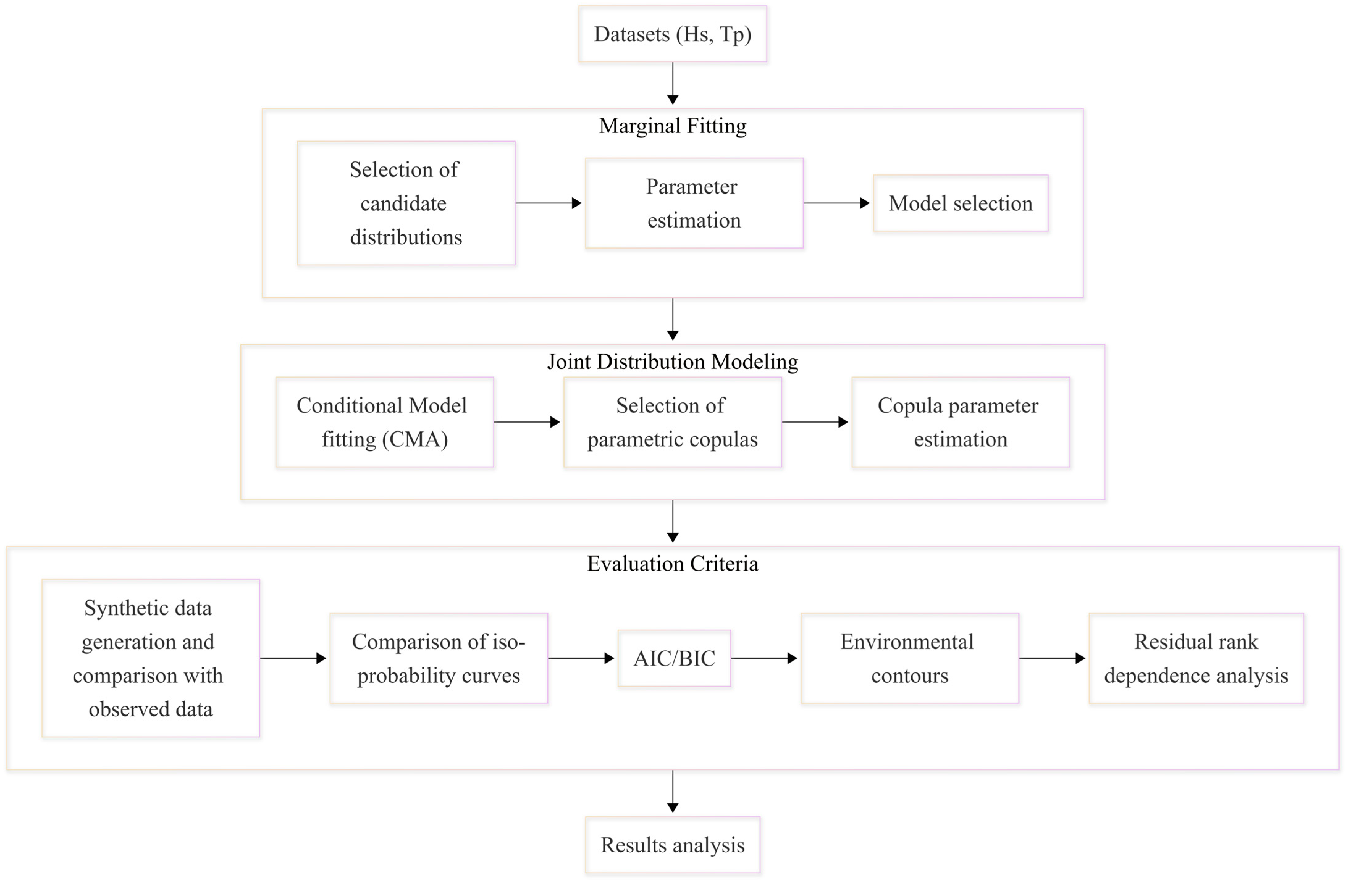
Figure 1 provides an overview of the modeling framework, summarizing the main steps from data input to model evaluation.

3.1. Description of Datasets

The data used in this study consist of historical wave hindcast series, with 3-h resolution, for the pairs ${(H}_s,T_p)$ covering a continuous 20-year period. The series are derived from two numerical modeling sources:

• Set 1 (C1): Data for the northern region of the Campos Basin, Brazil, generated from the MyOcean/Copernicus and ERA5 (ECMWF) databases, with validation via satellite data and GlobWave [25].
• Sets 2 and 3 (C2, C3): Data obtained from the WAVEWATCH III (WW3) model for two locations: Santos Basin (C2) and Equatorial Margin (C3) [26].

For each location, the wave records are separated into their sea and swell components. This separation results in six distinct modeling scenarios.

Table 3. Statistical characteristics of the datasets.

Component	Period	$\widehat{\mathit{\rho }}$	${\widehat{\mathit{\rho }}}_{\mathit{S}}$	$\widehat{\mathit{\tau }}$
C1-sea	1999–2018	0.97	0.99	0.92
C1-swell	1999–2018	0.73	0.70	0.51
C2-sea	2004–2024	0.56	0.54	0.39
C2-swell	2004–2024	0.13	0.09	0.07
C3-sea	2004–2024	0.26	0.24	0.17
C3-swell	2004–2024	0.16	0.11	0.07

summarizes the main sample dependence measures for each of the six scenarios. The wide variation observed in the dependence coefficients, ranging from very high values (C1-sea) to near-zero values (C2-swell, C3-swell), provides an ideal spectrum for evaluating model performance under different dependence regimes.

The near-zero dependence coefficients observed for the swell scenarios (C2-swell and C3-swell) in Table 3 are consistent with the wave energy dispersion mechanism described in the Introduction.

To complement the global dependence measures reported in Table 3,

Table 4. Empirical tail dependence coefficients.

Component	$\widehat{{\mathit{\lambda }}_{\mathit{L}}}$ ($\mathit{q} = 0.10$)	$\widehat{{\mathit{\lambda }}_{\mathit{U}}}$ ($\mathit{q} = 0.90$)
C1-sea	0.87	0.83
C1-swell	0.34	0.56
C2-sea	0.62	0.38
C2-swell	0.07	0.16
C3-sea	0.32	0.20
C3-swell	0.06	0.26

presents the empirical lower and upper tail dependence coefficients ($\widehat{{\lambda }_L}$ and $\widehat{{\lambda }_U}$, Equations (21) and (22)) estimated for all six scenarios at thresholds $q = 0.10$ (lower tail) and $q =0.90$ (upper tail). The results reveal that tail dependence is strongly correlated with the global dependence regime: C1-sea presents the highest values in both tails ($\widehat{{\lambda }_L}=0.87$; $\widehat{{\lambda }_U}=0.83$), consistent with its near-perfect global correlation. Notably, even in scenarios with near-zero global coefficients, such as C3-swell, non-negligible tail dependence persists ($\widehat{{\lambda }_U}=0.26$).

3.2. Fitting of Marginal Distributions

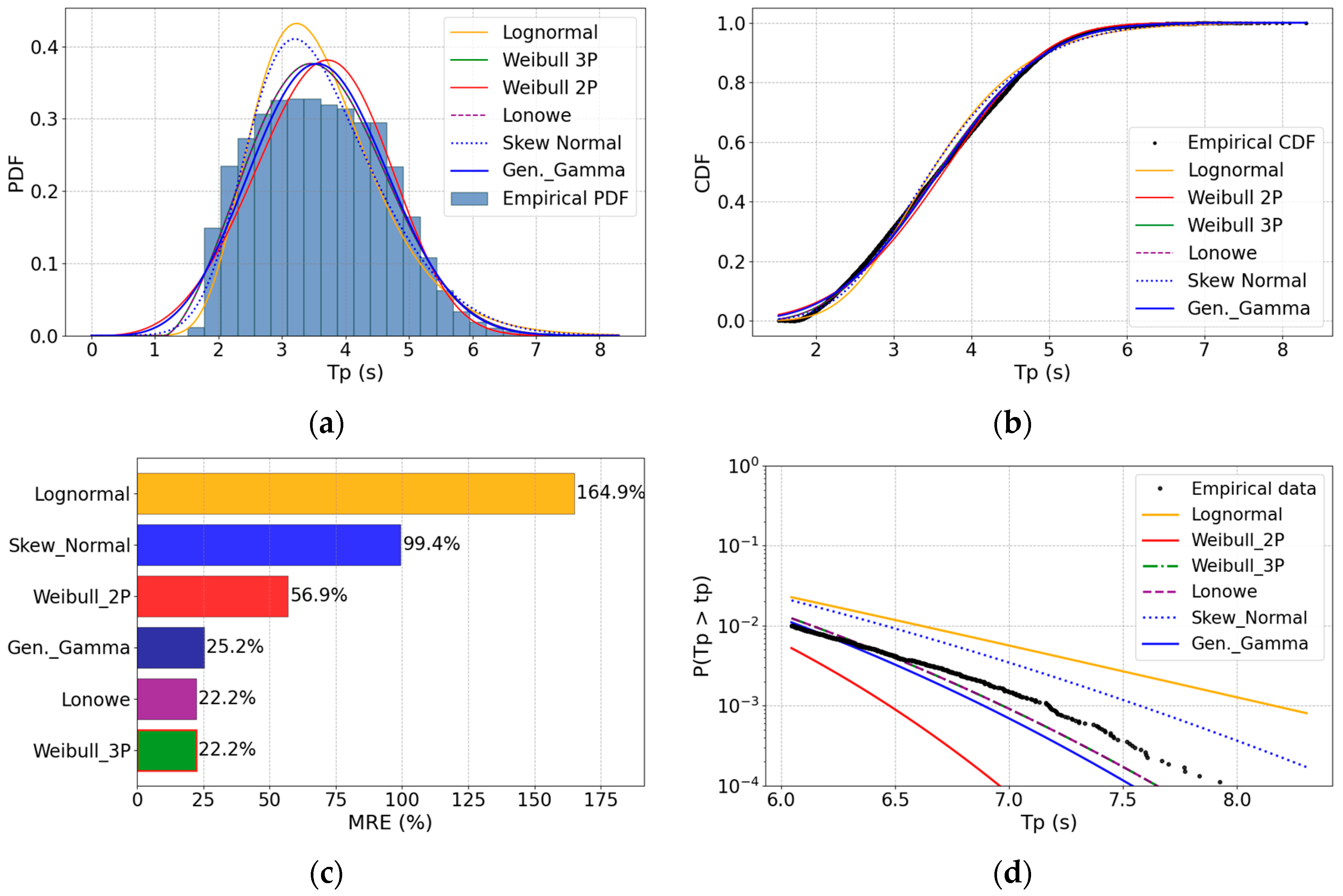
For each of the six data series, a set of candidate distributions, listed in Table 1, was fitted to $H_s$ and $T_p$ data individually. Parameter estimation was performed using both the method of moments and maximum likelihood.

The empirical distribution was obtained by partitioning the domain of variable $X$ into $M$ intervals of equal width $\Delta x=\left(x_{max}-x_{min}\right)/M$, where $M$ was determined by visual inspection for each dataset to ensure adequate resolution across the distribution domain and to maintain a sufficient number of observations per interval. For each interval $i$, centered at $x_i$, the empirical PDF is estimated as:

$${\widehat{f}}_X\left(x_i\right)=\frac{n_i}{n·\Delta x}$$

(26)

where $n_i$ denotes the number of observations falling within the $i$-th interval and $n$ is the total sample size. The corresponding empirical CDF is given by:

$${\widehat{F}}_X({\overline{x}}_j)=\frac{j}{n+1}$$

(27)

where ${\overline{x}}_j$ is the $j$-th element of the sampled values sorted in ascending order.

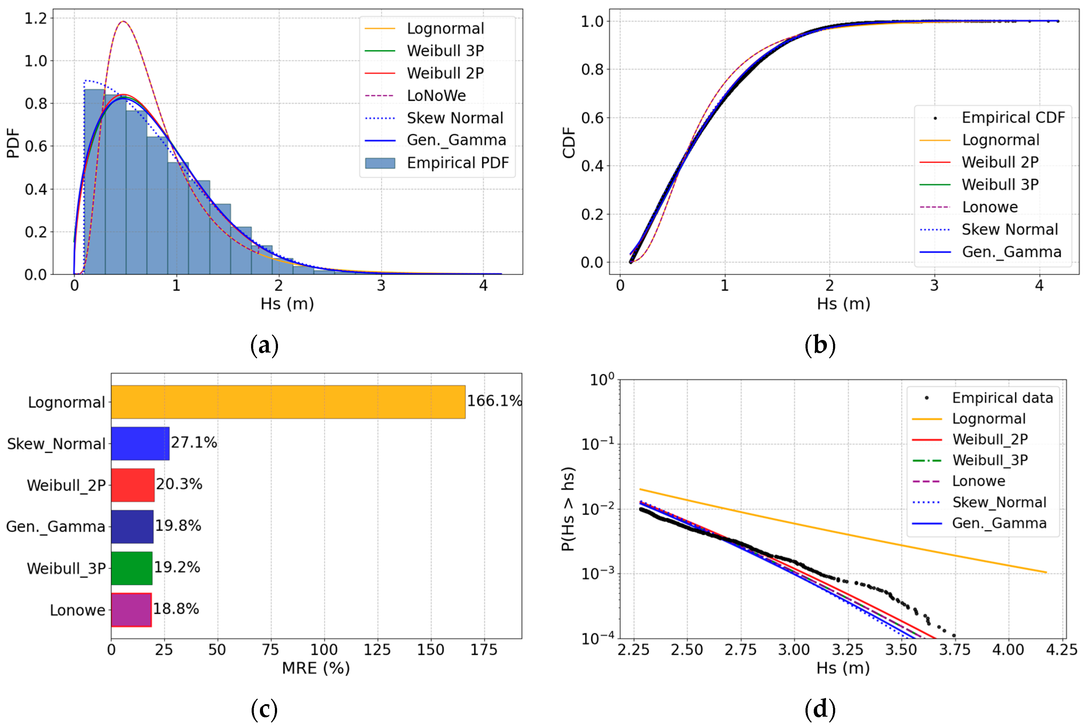
Model selection prioritized the quality of fit in the upper tail, as this region is critical for estimating extreme events in offshore engineering applications. For each candidate distribution, the mean relative error (MRE) was computed between the theoretical and empirical exceedance probabilities for four high quantiles: 95.0%, 99.0%, 99.5%, and 99.9%. The exceedance probability, also referred to as the survival function $S\left(x\right) = P(X > x) = 1 - F_X\left(x\right)$, provides a direct measure of the probability of observing values above a given threshold. For a given quantile $q$, the corresponding threshold is defined as $x_q={\widehat{F}}_X^{-1}\left(q\right)$. The empirical exceedance probability is $S_{emp}\left(x_q\right)=1-q$, while the theoretical exceedance probability is $S_{teo}\left(x_q\right)=1-F_X\left(x_q\right)$. The relative error for each quantile is calculated as:

$${RE}_q=\left|\frac{S_{teo}\left(x_q\right)-S_{emp}\left(x_q\right)}{S_{emp}\left(x_q\right)}\right|·100\%$$

(28)

The MRE is then obtained as the arithmetic mean of the errors across the four selected quantiles:

$$MRE=\frac{1}{4}\sum _{q\in Q}{RE}_q,\hspace{1em}\hspace{1em}Q=\left\{0.950; 0.990;0.995;0.999\right\}$$

(29)

The distribution exhibiting the lowest MRE, combined with visual assessment of the fitted PDFs, CDFs and survival function, was selected for each variable.

3.3. Modeling of the Joint Distribution

The joint distribution of $H_s$ and $T_p$ was modeled using two approaches: the CMA and copula theory.

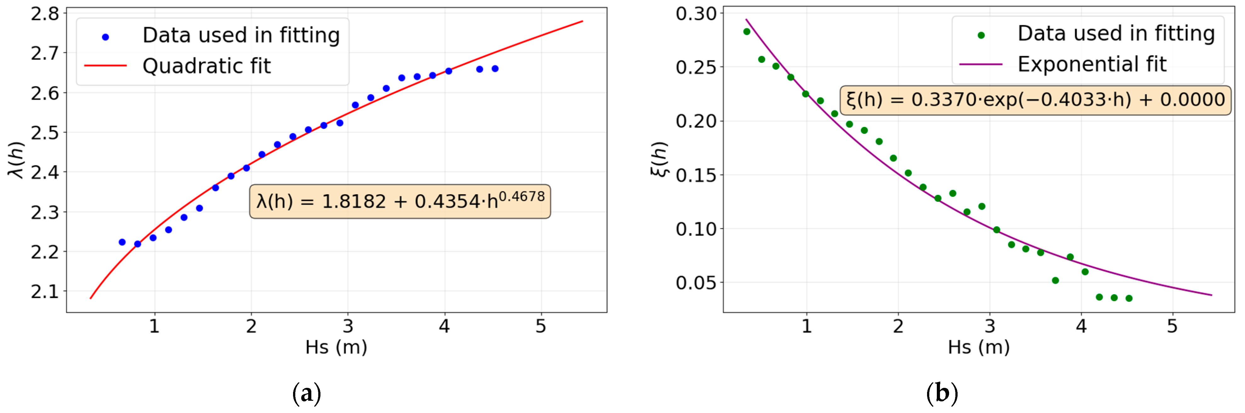
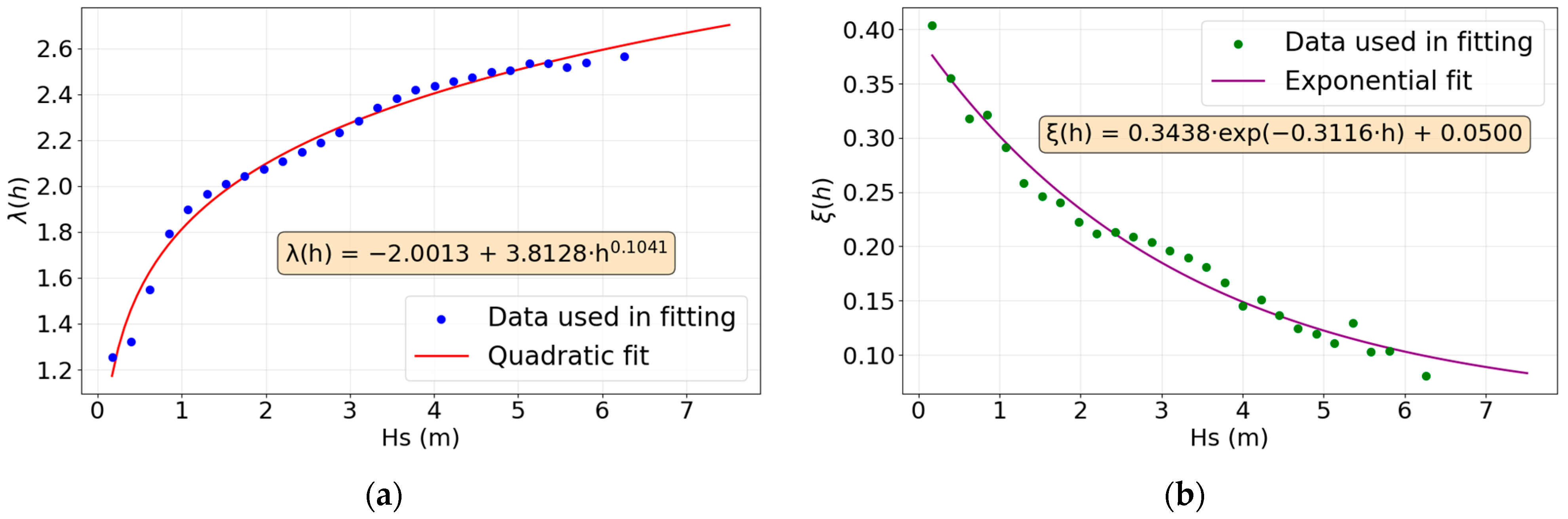
CMA: Following Equation (1), the joint PDF is given by the product of the marginal distribution of $H_s$ (Section 3.2) and the conditional distribution $T_p|H_s$, modeled as Lognormal with parameters $\lambda \left(h_s\right)$ and $\xi \left(h_s\right)$ (Equations (5) and (6)). The coefficients $a_i$ and $b_i$ were estimated using nonlinear least squares from the values of λ and ξ computed within $H_s$ intervals, where the number of intervals was determined by visual inspection for each scenario, with outlying point estimates removed before the fitting procedure. To ensure the positivity of $\xi \left(h_s\right)$, the constraints $b_1, b_3\ge 0$ were imposed during the fitting procedure, with $b_1+b_3> 0$ as a sufficient condition for $\xi \left(h_s\right)> 0$ across the entire $H_s$ domain.

Copulas: The data were transformed into uniform pseudo-observations $u_i=F_{H_s}\left(h_{s_i}\right)$ and $v_i=F_{T_p}\left(t_{p_i}\right)$ in the interval $[0,1]$. Eight families of copulas were fitted, as listed in Table 2: Gaussian, Student’s t, Gumbel, Clayton, Frank, Joe, BB1, and Plackett. Parameters were estimated using both the method of moments and maximum likelihood via the IFM (see Section 2.5). The eight families selected represent the most widely adopted parametric copulas in offshore and coastal engineering applications [1,15,16,17,18]. More flexible structures, such as non-parametric copulas and mixture copulas, are outside the scope of this baseline study but are identified as important directions for future research.

It should be noted that the CMA and the parametric copulas operate under structurally asymmetric parameterizations. The CMA employs six free parameters to describe the conditional distribution of $T_p$ given $H_s$ (Equations (5) and (6)), while most single-parameter copula families use one parameter to characterize the entire dependence structure. A strictly equivalent comparison would require either two-parameter copula families, such as the BB1 or Student’s t, already included in this study, or more flexible constructions such as mixture copulas with comparable degrees of freedom.

3.4. Evaluation Criteria

It is recognized that selecting the most appropriate joint distribution model is challenging, even for bivariate problems [13]. The performance of the models was evaluated using four complementary criteria:

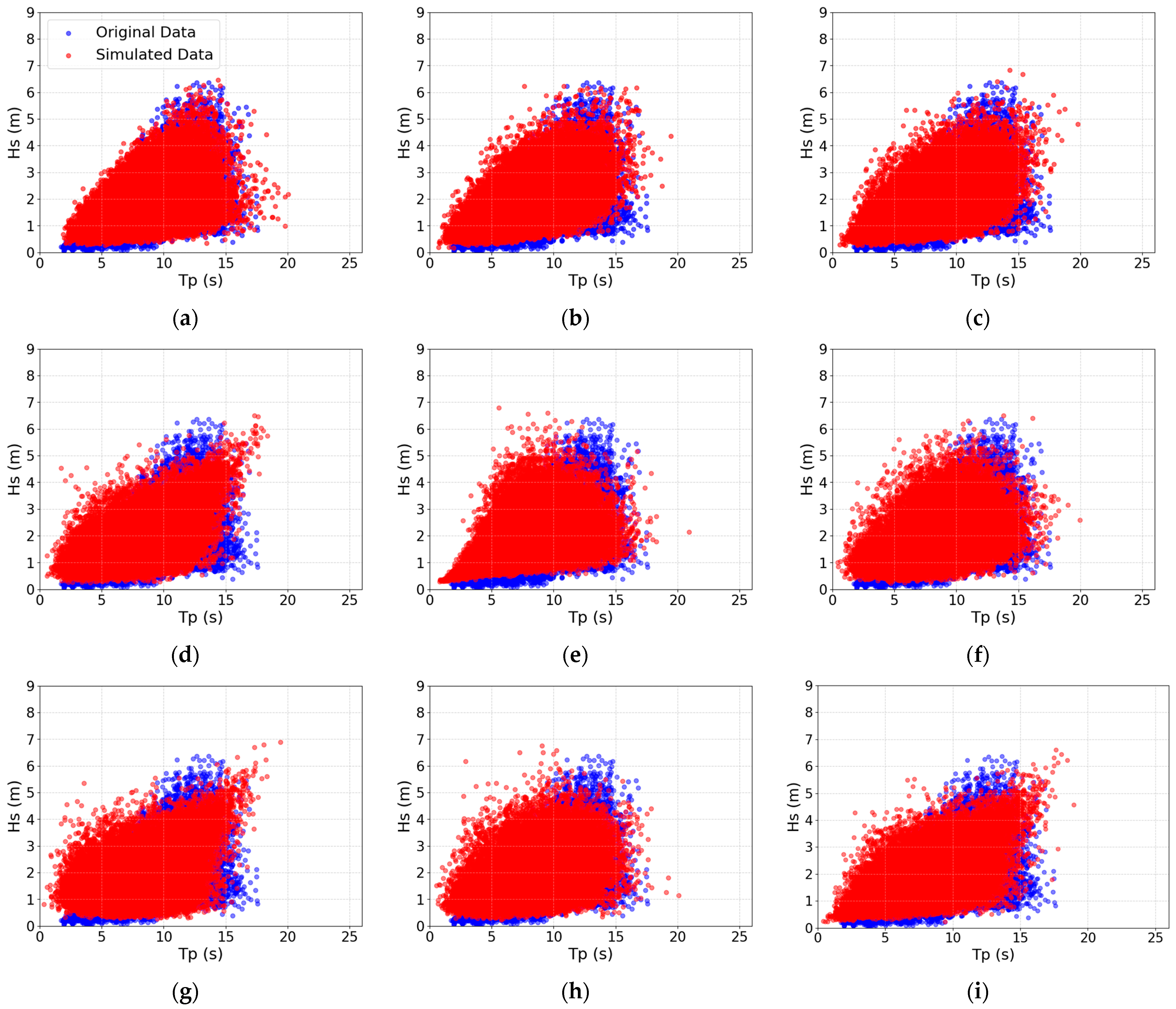
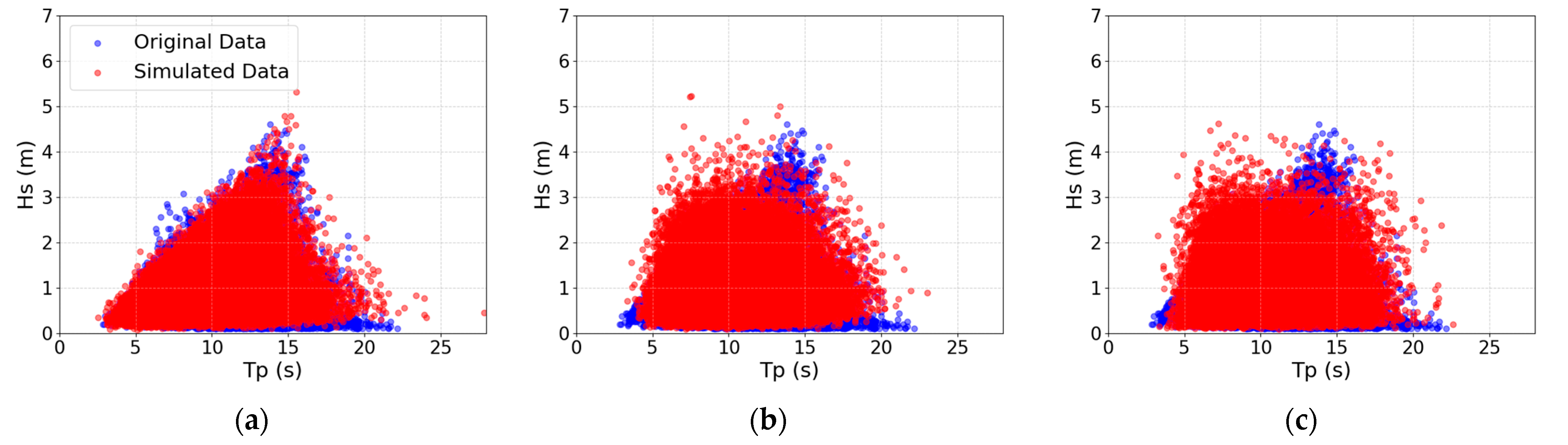
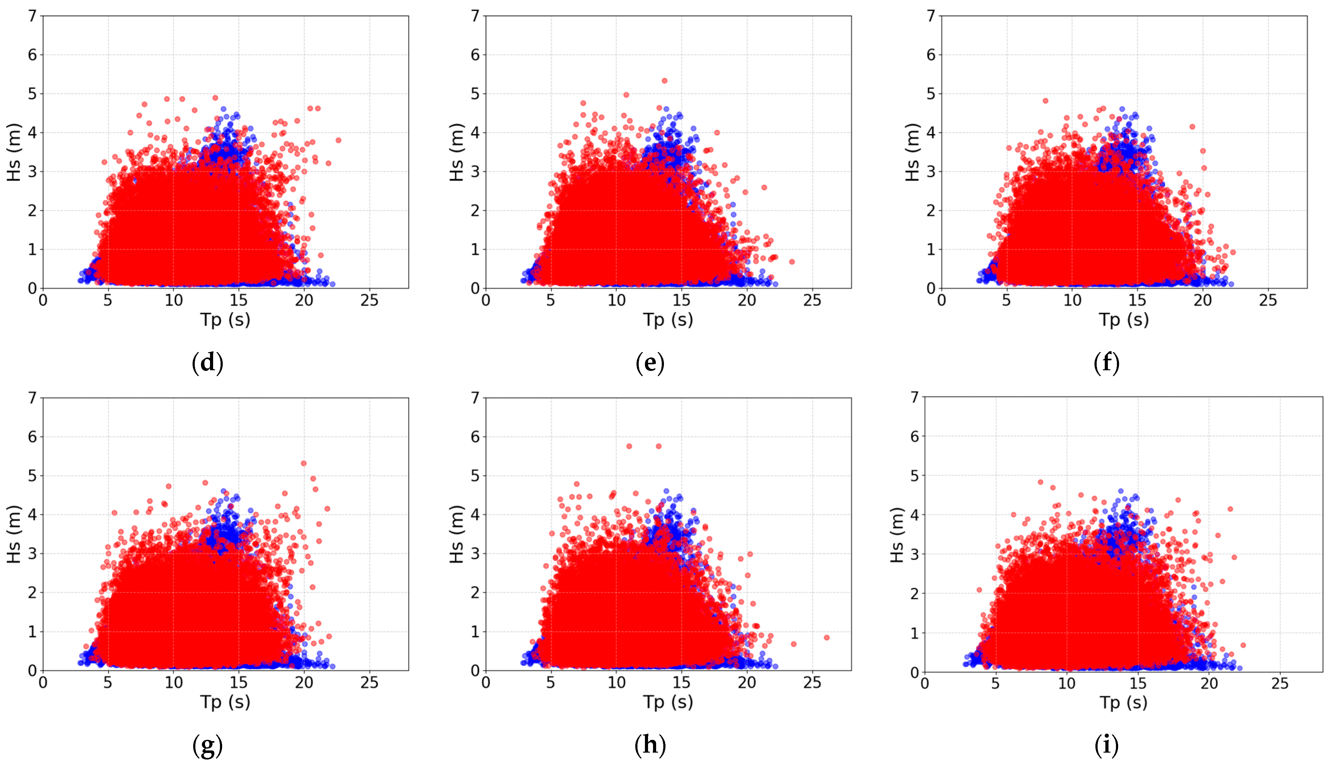
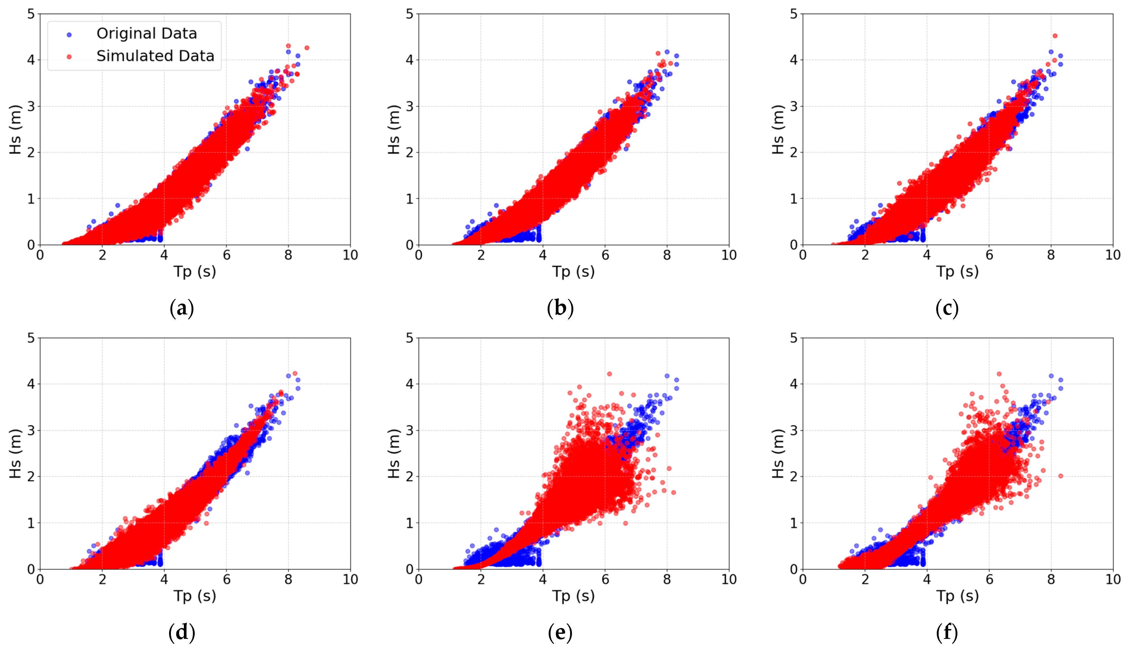
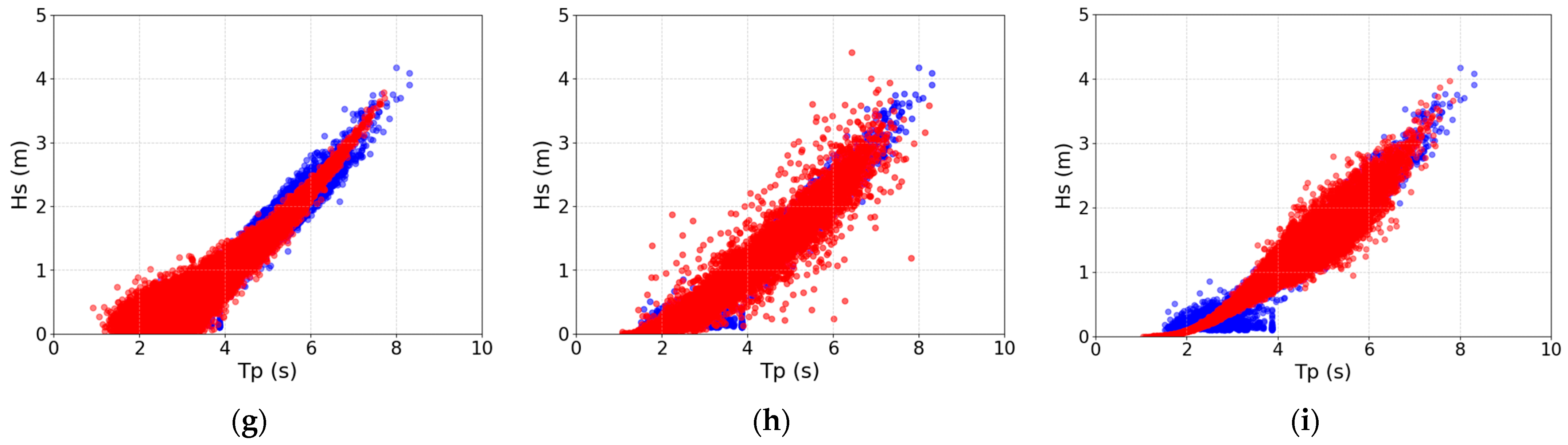
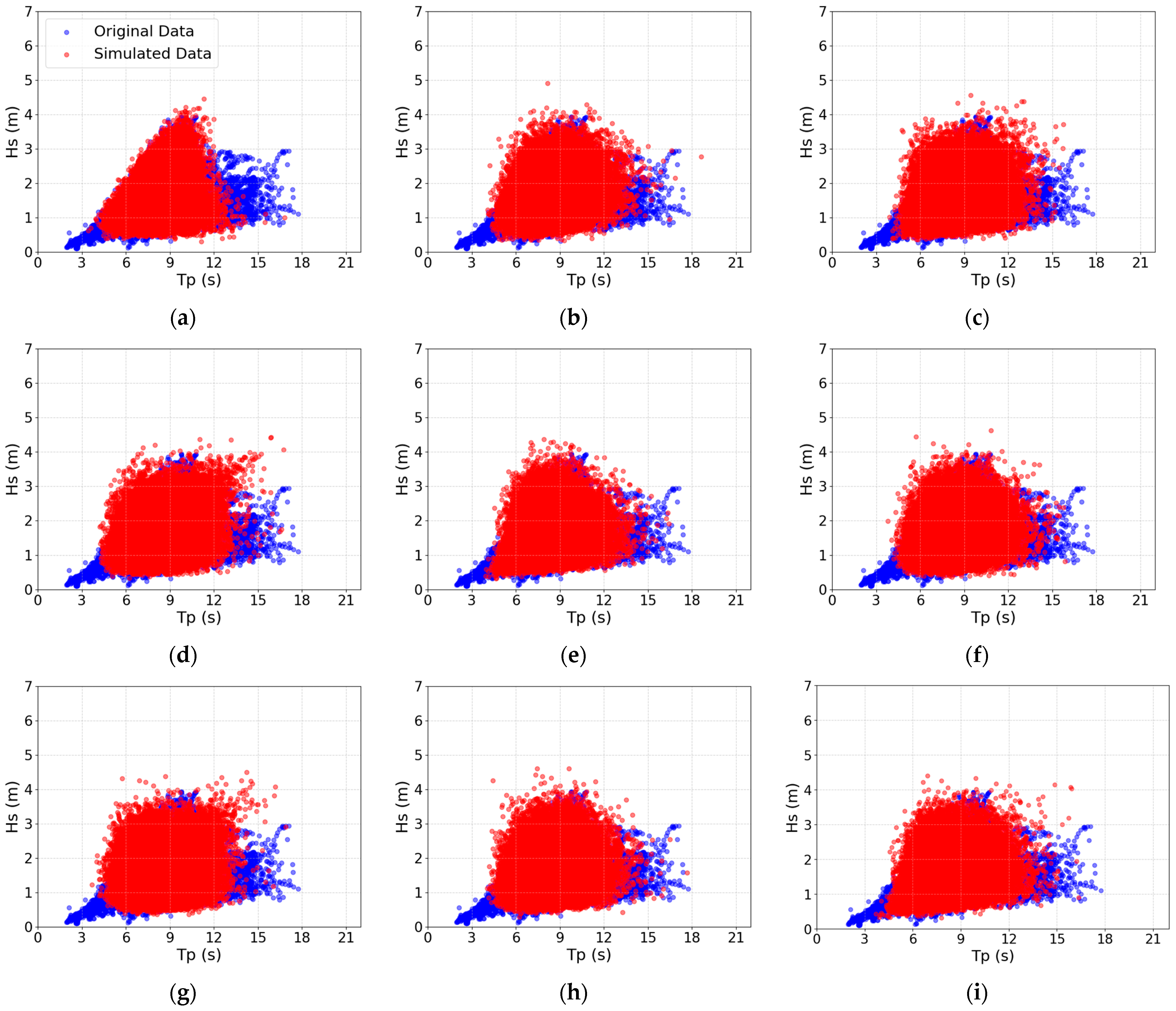
• For each fitted model, a synthetic sample of the same size as the original dataset was generated via Monte Carlo Simulation. The synthetic scatter plots were visually compared to the observed data.
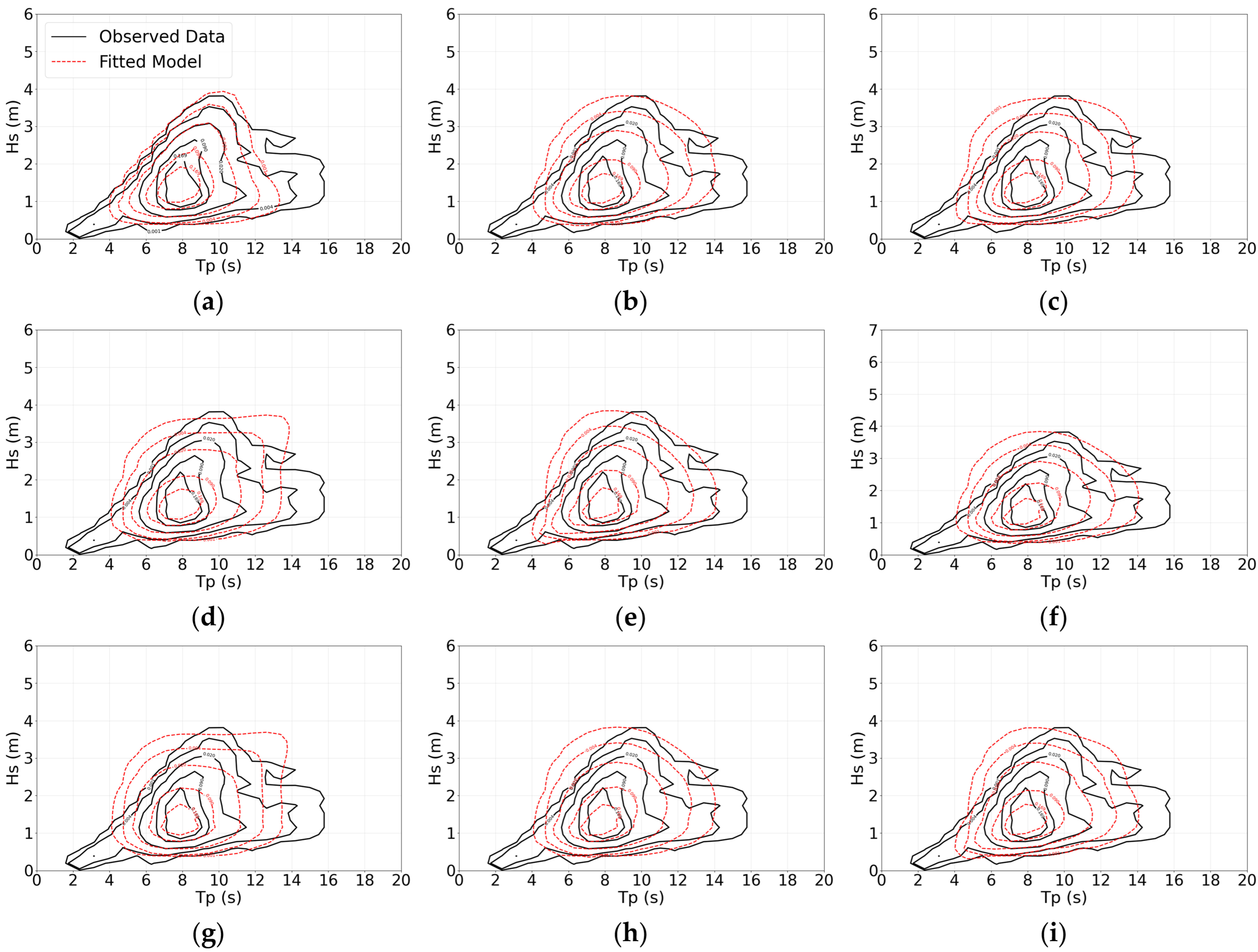
• The empirical joint PDF of the observed data was estimated using two-dimensional histograms with the following formulation:

$$f_{H_s{T}_p}\left(h_i,t_j\right)=\frac{n_{i,j}}{n_{total}·\Delta h·\Delta t}$$

(30)

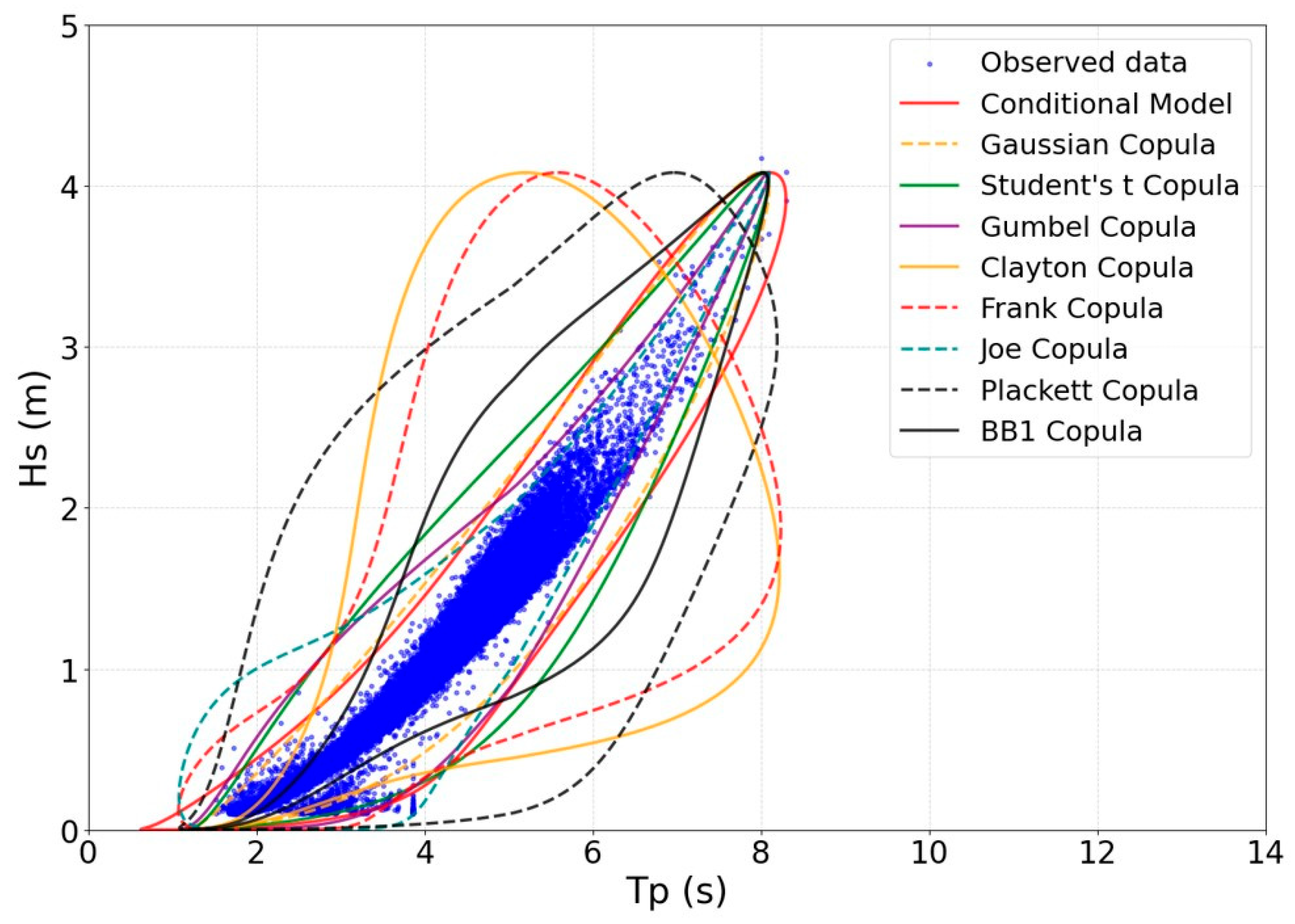
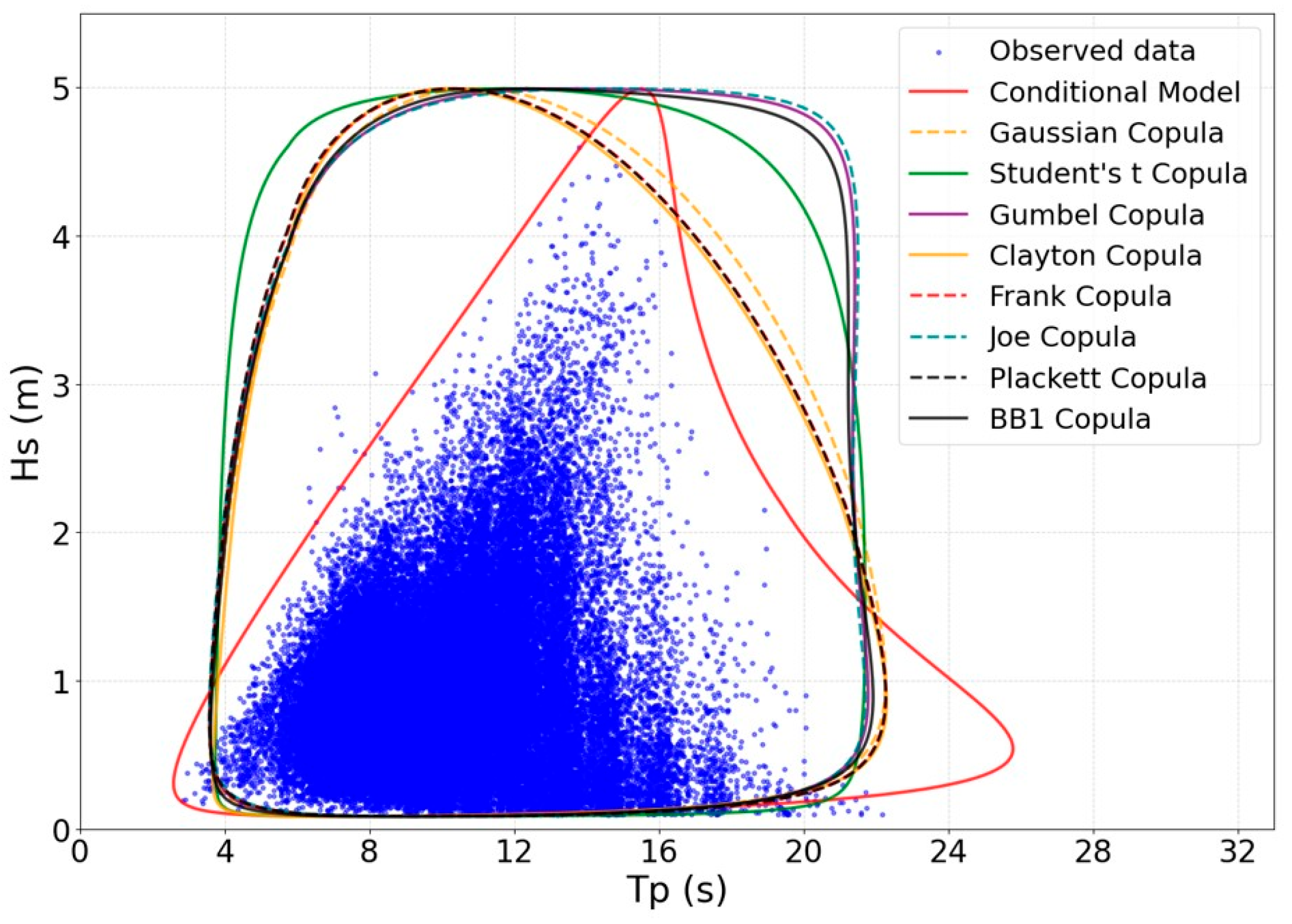
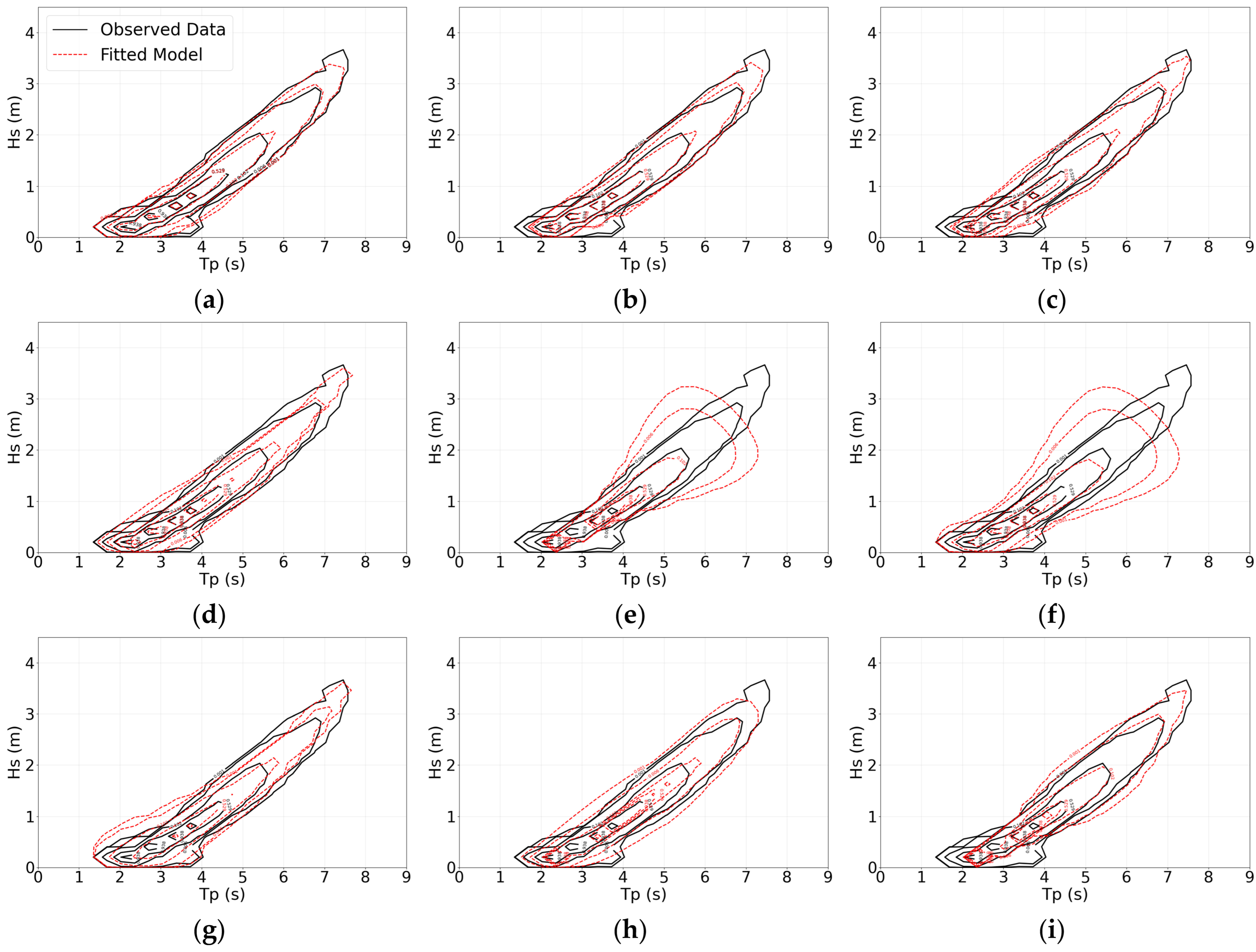
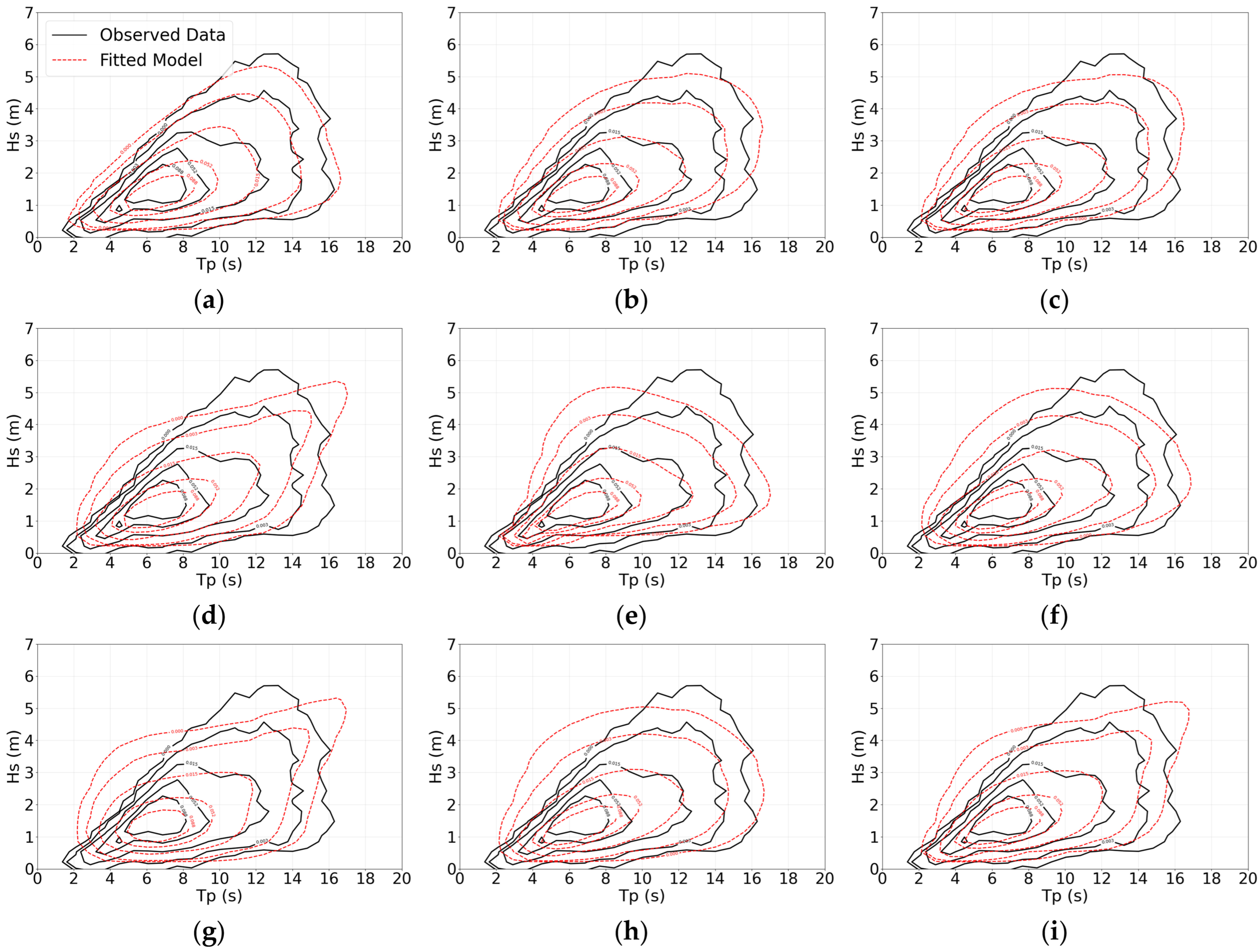
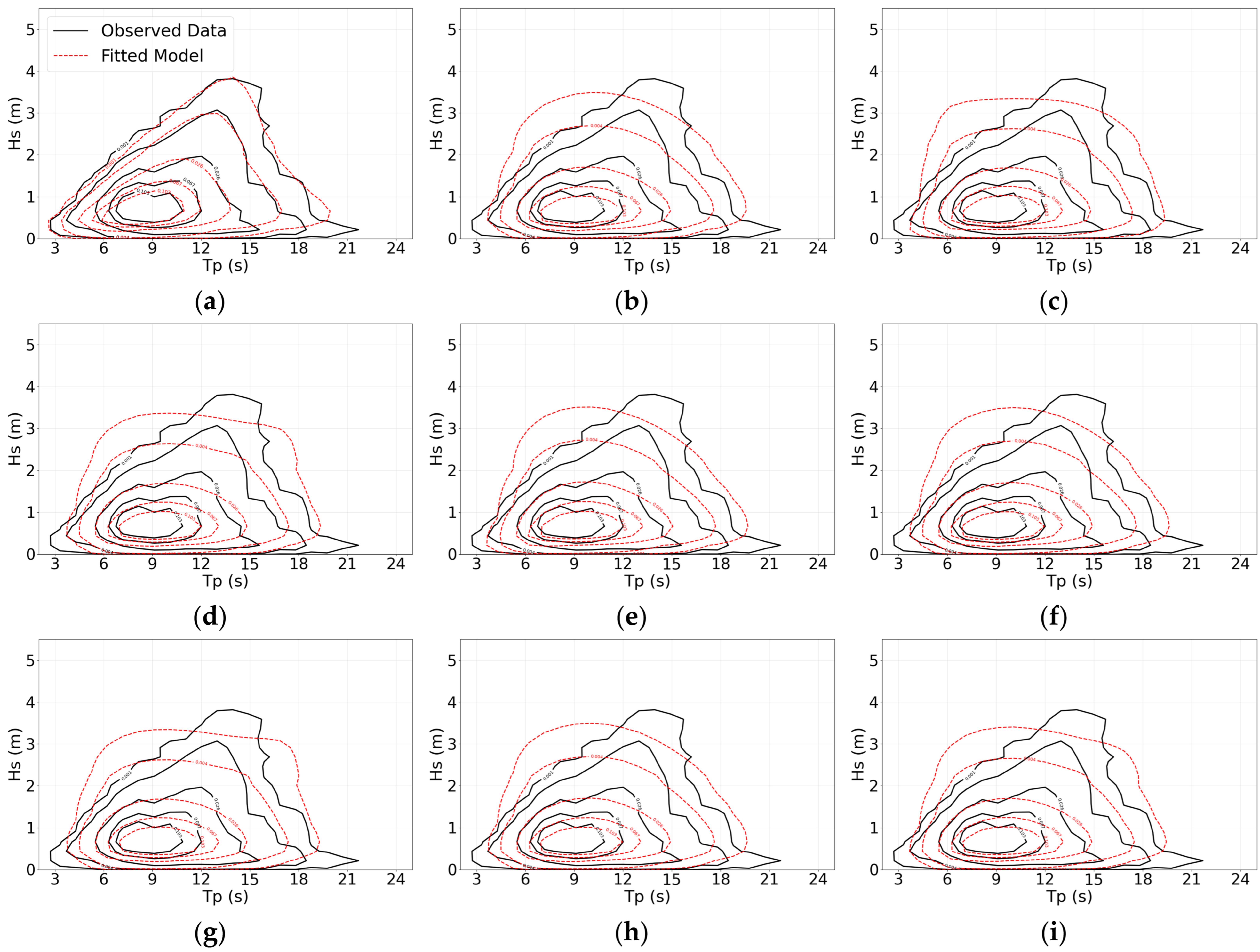
where $n_{i,j}$ is the number of observations contained in the cell $\left(i,j\right)$, $n_{total}$ is the total number of points, and $\Delta h$ and $\Delta t$ are the interval widths. For each fitted model, the theoretical joint PDF was obtained directly from Equation (1) for the CMA and from Equation (14) for the copula models. The theoretical and empirical PDFs were then visually compared through the iso-probability curves.

iii.

Akaike Information Criterion (AIC) [27] and Bayesian Information Criterion (BIC) [28]: these approaches were used as relative measures of goodness-of-fit, penalizing model complexity:

$$AIC=2k-2{\displaystyle \sum _{i=1}^n}\ln \left[f_{X,Y}\left(x_i,y_i;\mathit{\theta },\mathit{\alpha },\mathit{\beta }\right)\right]$$

(31)

$$BIC=k\ln \left(n\right)-2{\displaystyle \sum _{i=1}^n}\ln \left[f_{X,Y}\left(x_i,y_i;\mathit{\theta },\mathit{\alpha },\mathit{\beta }\right)\right]$$

(32)

where $k$ is the total number of parameters (marginal $+$ copula parameters). Lower values indicate a better balance between fit and simplicity.

iv.

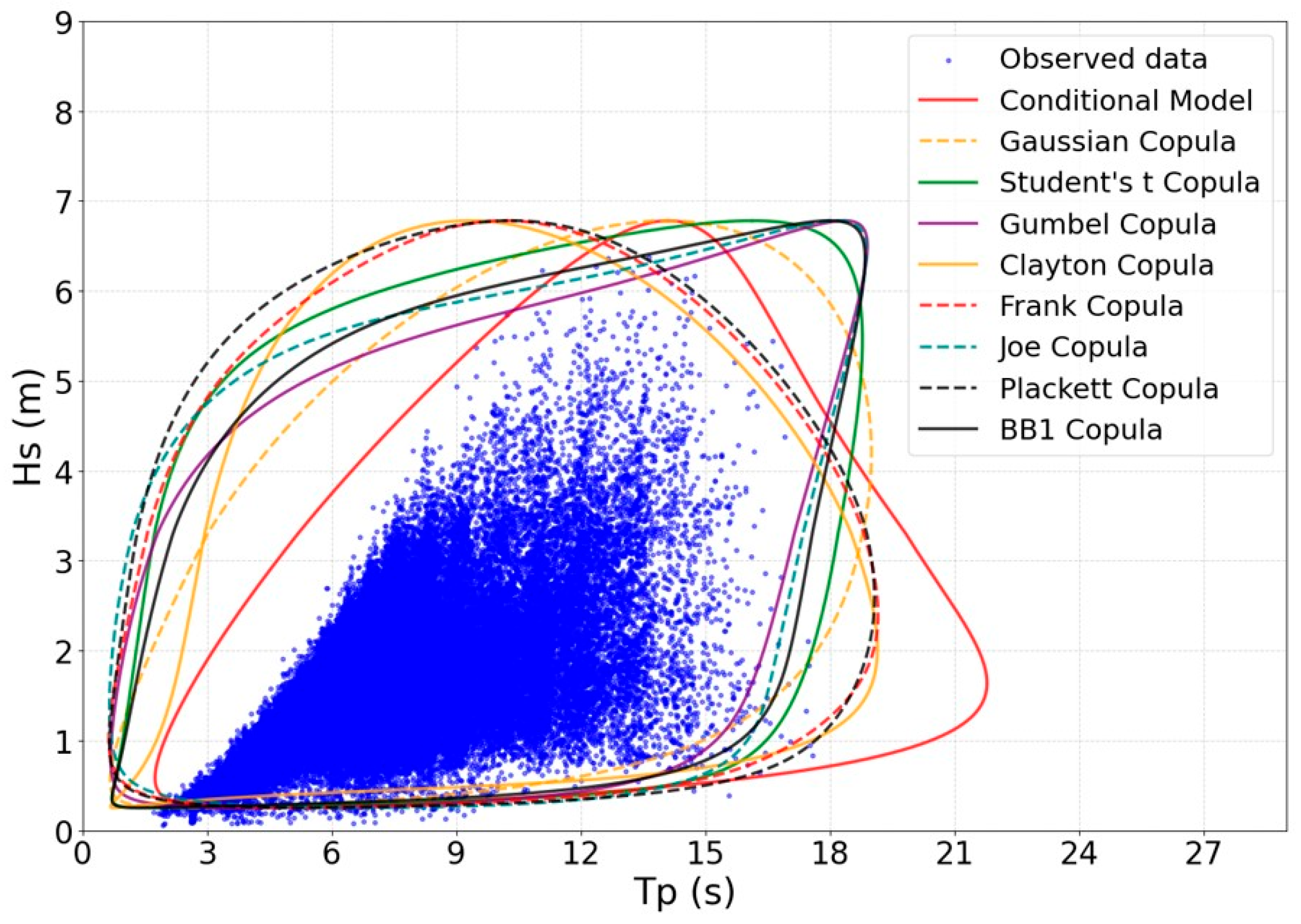
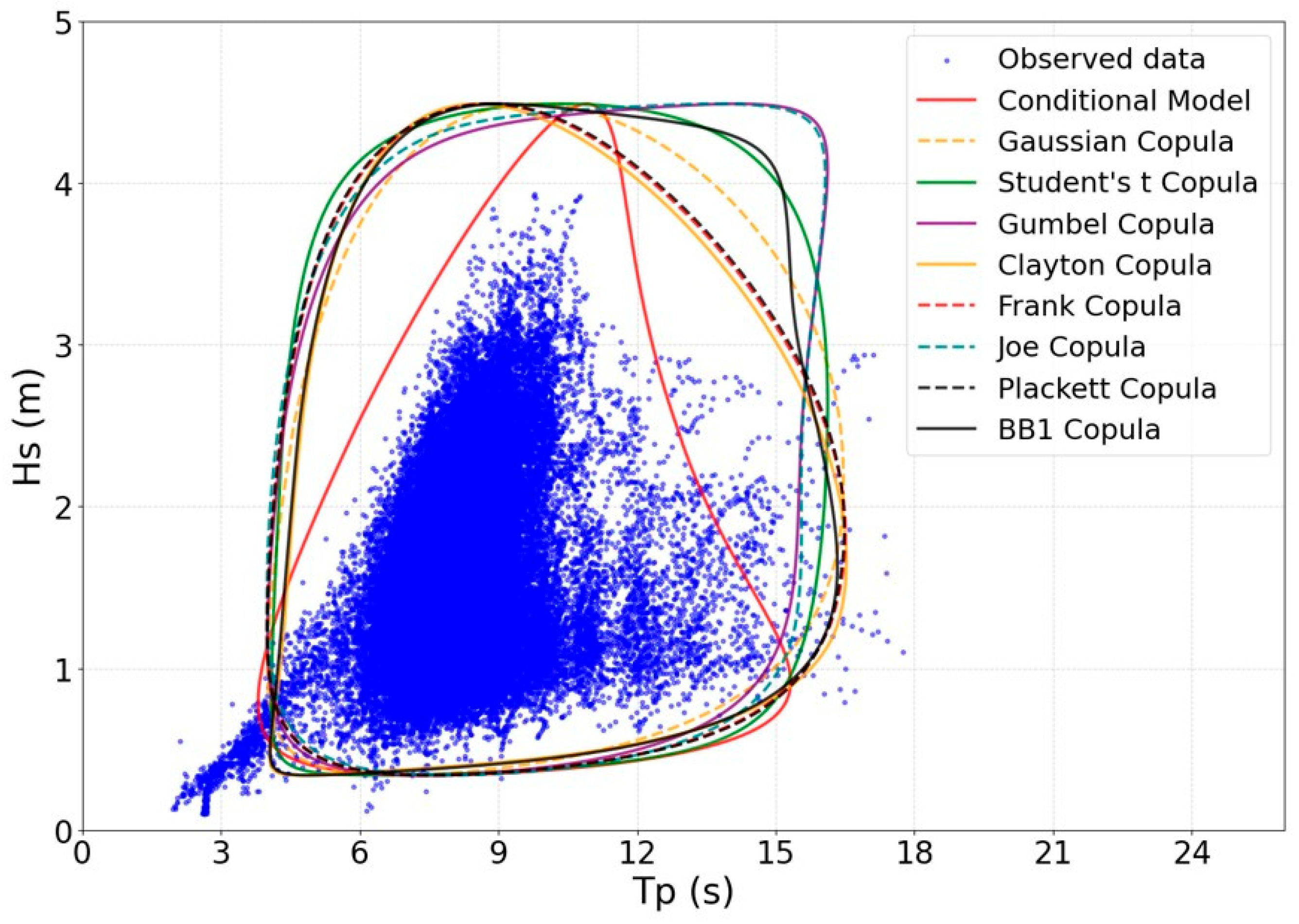
Environmental contours: these were constructed for a 20-year return period using the IFORM method [29], allowing validation of the models against the observed data. The reliability index $\beta$ associated with the return period $T_r$ is given by:

$$\beta ={\Phi }^{-1}\left(1-\frac{1}{N_{1-year}·T_r}\right)$$

(33)

where $N_{1-year}=2920$ is the expected number of short-term sea states in one year, considering a 3-h time discretization, and ${\Phi }^{-1}\left(·\right)$ denotes the inverse of the standard normal CDF, with $\Phi \left(·\right)$ representing the standard normal CDF itself. Standard Gaussian directions $U_1=\beta \cos \left(\vartheta \right), U_2=\beta \sin \left(\vartheta \right), \vartheta =\left(0,2\pi \right)$, generate a circle of radius $\beta$ in the bivariate standard normal space, which is mapped back to the physical space as follows:

• CMA:

$$H_s=F_{H_S}^{-1}\left[\Phi \left(U_1\right)\right], T_p=F_{T_p|H_s}^{-1}\left[\Phi \left(U_2\right)|H_s\right];$$

(34)

• Copulas:

$$Z_1=\Phi \left(U_1\right), { Z}_2=C_{2|1}^{-1}\left[\Phi \left(U_2\right)|H_s\right],\hspace{1em}\hspace{1em}with H_s=F_{H_S}^{-1}\left(Z_1\right), { T}_p=F_{T_p}^{-1}\left(Z_2\right)$$

(35)

It is worth noting that the IFORM construction relies on a Rosenblatt-like transformation [30] requiring a well-behaved inverse of the conditional copula CDF; alternative contour methods such as direct-sampling or ISORM approaches [6] are outside the scope of this study.

When the criteria do not fully agree, a hierarchical decision protocol is applied: physical plausibility of the synthetic scatter plot serves as a primary filter; structural adherence of iso-probability curves as a secondary filter; tail behavior in environmental contours as a tertiary criterion; and finally, AIC/BIC as an auxiliary discriminator among models that pass the preceding filters. When AIC/BIC contradicts the visual ranking, the visual criteria are prioritized due to their direct relevance to engineering design, particularly in applications such as the derivation of environmental contours for offshore structural design.

As a complementary criterion, a residual rank dependence analysis was conducted for selected scenarios based on the Rosenblatt probability integral transform, as detailed in Section 4.3.5. This analysis quantifies the dependence structure not captured by each fitted model in the rank domain and provides an additional perspective on model adequacy independent of the visual and likelihood-based criteria described above.

Regarding computational effort, the CMA and the parametric copula fitting procedures are computationally tractable for the dataset sizes considered. Computational efficiency was not a limiting factor in any scenario, and its influence on model selection is negligible compared to the differences in statistical robustness. All analyses were implemented in Python (version 3.12.13).

4. Results and Discussion

4.1. Fitting of Marginal Distributions

Figure 2 and Figure 3 illustrate, as an example, the selection process of marginal distributions for the variables $H_s$ and $T_p$ for sea component in Set 1 (C1-sea). For $H_s$ (Figure 2) the Weibull 2P distribution was selected based on the combined MRE and visual assessment. Although the MRE values of Weibull 2P (20.3%) and Lonowe (18.8%) are comparable, the Weibull 2P showed superior adherence to the observed data across both the body of the distribution and the upper tail region, as evidenced by the survival function plot in Figure 2d. For $T_p$ (Figure 3) the Lonowe distribution stood out with the lowest MRE (22.2%) and excellent fit in the upper tail.

Table 5. Selected marginal distributions for the $H_s$ and $T_p$ variables.

Component	Variable	Distribution
C1-sea	$H_s$	Weibull 2P
C1-sea	$T_p$	Lonowe
C1-swell	$H_s$	Lonowe
C1-swell	$T_p$	Lonowe
C2-sea	$H_s$	Lonowe
C2-sea	$T_p$	Generalized Gamma
C2-swell	$H_s$	Lonowe
C2-swell	$T_p$	Lonowe
C3-sea	$H_s$	Lonowe
C3-sea	$T_p$	Lognormal
C3-swell	$H_s$	Lonowe
C3-swell	$T_p$	Lonowe

summarizes the selected marginal distributions for all scenarios. Lonowe was the most frequently selected distribution. The Generalized Gamma and Lognormal distributions were only selected for $T_p$ in C2-sea and C3-sea, respectively. For $H_s$, Lonowe predominated, except for C1-sea (Weibull 2P).

4.2. Fitting of the Joint Distribution

In the CMA, the coefficients of the parametric functions $\lambda \left(h_s\right)$ and $\xi \left(h_s\right)$ (Equations (5) and (6)) were estimated for each scenario. As an example, Figure 4 and Figure 5 illustrate the fitting for Set C2 for the sea and swell components. The fitted curves showed good agreement with the point estimates.

Table 6. Parameters of the fitted copulas.

Component	Gaussian $\left(\mathit{\rho }\right)$	t-Student $(\mathit{\rho };\mathit{\nu })$	Gumbel $\left(\mathit{\theta }\right)$	Clayton $\left(\mathit{\theta }\right)$	Frank $\left(\mathit{\theta }\right)$	Joe $\left(\mathit{\theta }\right)$	BB1 $(\mathit{\theta };\mathit{\delta })$	Plackett $\left(\mathit{\theta }\right)$
C1-sea	${0.98}^{ *}$	${\left(0.98; 9.42\right) }^{*}$	${6.45}^{ *}$	$24.30$	$50.91$	${8.88 }^{*}$	$(8.75; 2.45)$	$1000.46$
C1-swell	$0.72$	$(0.72; 11.18)$	$2.05$	$2.11$	$5.98$	${2.33}^{ *}$	$(0.26; 1.82)$	$13.05$
C2-sea	$0.57$	$(0.57; 24.62)$	$1.64$	$1.28$	$4.02$	${1.57}^{ *}$	$(0.27; 1.44)$	$5.97$
C2-swell	$0.10$	$(0.10; 10.74)$	$1.07$	$0.14$	$0.60$	${1.08}^{ *}$	$(0.04; 1.05)$	$1.30$
C3-sea	$0.26$	$(0.26; 14.02)$	$1.19$	$0.39$	$1.52$	${1.09}^{ *}$	$(0.33; 1.03)$	$2.06$
C3-swell	$0.11$	$(0.11; 12.59)$	$1.08$	$0.16$	$0.66$	${1.18}^{ *}$	$(0.01; 1.14)$	$1.37$

* Indicates that the parameter was estimated via IFM. All other parameters were estimated via the method of moments.

summarizes the estimated parameters for the eight copula families in each scenario, obtained by the method of moments and maximum likelihood (IFM). In general, the estimated parameters by both methods were quite similar. In the few cases where the estimates diverged, the most appropriate set of parameters was selected based on visual inspection, prioritizing the model that best captured the observed statistical dependence structure. It can be observed that the parameters consistently reflect the intensity of the dependence coefficients: high values for C1-sea and values close to zero in the low dependence coefficient scenarios (C2-swell, C3-swell).

4.3. Analysis by Dependence Coefficient Levels

Based on the fitted models, a comparative performance analysis is presented for each regime of dependence coefficient magnitude (Table 3), integrating the four evaluation criteria described in Section 3.4.

4.3.1. High Dependence Coefficient Levels

Set C1 in the sea wave component (C1-sea) presents the highest dependence coefficients among all scenarios (Table 3). In this context, the CMA and the elliptical copulas (Gaussian and Student’s t) showed superior and equivalent performance, reproducing with high fidelity the observed scatter plot and the iso-probability curves throughout the data domain, as illustrated in Figure 6 and Figure 7. The environmental contours generated for the 20-year return period (Figure 8) show that the CMA and the Gaussian copula almost perfectly coincide with the boundary of the observed data. The Student’s t copula, although visually close, presented small distortions in the environmental contour in the central region. The choice of the joint probability distribution model may consider the type of structural analysis to be performed and the structure’s dynamic behavior. In general terms, for fatigue analysis, for example, accuracy in the central region perhaps is most relevant; on the other hand, for extreme responses, accuracy in the distribution tails can be more critical [2,5]. In practice, however, a single model is often sought for all structural analyses. In this context, the CMA and the Gaussian and Student’s t copulas accurately represented both the central region and the upper tail, making them suitable for both purposes. The Gumbel, Joe, and BB1 copulas reasonably reproduced the central region of the distribution but underestimated the upper tail, resulting in non-conservative contours for long return periods. Thus, while they may be adequate for fatigue, their use for extreme responses requires caution. The Clayton, Frank, and Plackett copulas showed unsatisfactory performance, with synthetic scatter plots clearly distinct from the observed one, distorted iso-probability curves, and environmental contours encompassing physically improbable regions, limiting their applicability for both fatigue and extreme analyses.

The AIC and BIC criteria (

Table 7. AIC and BIC information criteria for C1-sea—high dependence coefficients scenario.

Model	AIC	BIC
Conditional Model	$\mathrm{44,875.32}$	$\mathrm{44,946.39}$
Gaussian Copula	$\mathrm{39,621.05}$	$\mathrm{39,701.01}$
Student’s t Copula	$\mathrm{58,457.36}$	$\mathrm{58,546.20}$
Gumbel Copula	$\mathrm{56,970.91}$	$\mathrm{57,050.87}$
Clayton Copula	$\mathrm{313,557.89}$	$\mathrm{313,637.85}$
Frank Copula	$\mathrm{60,565.97}$	$\mathrm{60,645.93}$
Joe Copula	$\mathrm{76,332.28}$	$\mathrm{76,412.24}$
Plackett Copula	$\mathrm{84,996.76}$	$\mathrm{85,076.72}$
BB1 Copula	$\mathrm{68,666.58}$	$\mathrm{68,790.96}$

) confirmed the performance of the Gaussian copula in this scenario, which presented the lowest index values, followed by the CMA. The remaining copulas exhibited significantly higher values, in agreement with the visual analyses. Among these, the Clayton copula stands out with notably higher AIC and BIC values (313,557.89 and 313,637.85, respectively), a reflection of its poor fit to the high dependence structure of C1-sea, consistent with the distorted scatter plots and physically improbable environmental contour observed.

4.3.2. Moderate Dependence Coefficient Levels

The moderate dependence coefficients scenarios encompass the swell wave component of Set C1 (C1-swell), which presents moderate-high dependence coefficients ($\widehat{\rho }=0.73; \widehat{\tau }=0.51; {\widehat{\rho }}_S=0.70$), and the sea wave component of Set C2 (C2-sea), with typical moderate magnitude coefficients ($\widehat{\rho }=0.56; \widehat{\tau }=0.39; {\widehat{\rho }}_S=0.54$), as per Table 3. For C1-swell, the CMA and elliptical copulas showed superior and equivalent performance across all evaluation criteria, following the same pattern observed for C1-sea (Section 4.3.1), with the Gumbel, Joe, and BB1 copulas underestimating the upper tail and the Clayton, Frank, and Plackett copulas proving inadequate.

For C2-sea, the scatter plots and iso-probability curves (Figure 9 and Figure 10) show that the CMA remained the most robust, faithfully reproducing the observed statistical dependence structure throughout the data domain, making it suitable for both fatigue and extreme analyses. The elliptical copulas showed satisfactory performance in the scatter plots and iso-probability curves, with a slight limitation in the extreme regions, where the synthetic data either exceeded or underestimated the observed bounds, resulting in small distortions in the iso-probability curves. The remaining copulas showed unsatisfactory performance, limiting their applicability for structural design purposes. The environmental contours for the 20-year return period (Figure 11) show that the CMA and the Gaussian copula almost coincide with the boundary of the observed data. The Student’s t, Gumbel, Joe, and BB1 copulas exhibited a similar shape, with distortions in the central region and the upper tail, making them unsuitable for extreme response analyses. The remaining copulas presented contours that delimit regions encompassing unobserved parameter combinations, with shapes that do not correspond to the data structure.

The AIC and BIC criteria (

Table 8. AIC and BIC information criteria for moderate dependence coefficients scenarios.

Model	C1-Swell		C2-Sea
	AIC	BIC	AIC	BIC
Conditional Model	$\mathrm{224,612.19}$	$\mathrm{224,719.90}$	$\mathrm{375,902.39}$	$\mathrm{376,010.10}$
Gaussian Copula	$\mathrm{230,095.64}$	$\mathrm{230,212.32}$	$\mathrm{383,843.05}$	$\mathrm{383,959.74}$
Student’s t Copula	$\mathrm{228,994.08}$	$\mathrm{229,119.74}$	$\mathrm{383,197.92}$	$\mathrm{383,323.58}$
Gumbel Copula	$\mathrm{225,035.34}$	$\mathrm{225,152.02}$	$\mathrm{388,699.06}$	$\mathrm{388,815.74}$
Clayton Copula	$\mathrm{274,878.19}$	$\mathrm{274,994.87}$	$\mathrm{395,498.50}$	$\mathrm{395,615.18}$
Frank Copula	$\mathrm{225,422.74}$	$\mathrm{225,539.42}$	$\mathrm{387,724.97}$	$\mathrm{387,841.65}$
Joe Copula	$\mathrm{228,228.30}$	$\mathrm{228,344.98}$	$\mathrm{395,651.88}$	$\mathrm{395,768.57}$
Plackett Copula	$\mathrm{226,388.55}$	$\mathrm{226,505.24}$	$\mathrm{387,162.63}$	$\mathrm{387,279.31}$
BB1 Copula	$\mathrm{235,005.91}$	$\mathrm{235,131.57}$	$\mathrm{390,060.95}$	$\mathrm{390,186.61}$

) ratify the performance of the CMA in both scenarios, since this modelling approach presented the lowest index values. For C2-sea, the elliptical copulas rank next to the CMA, in agreement with the visual analyses, while the remaining copulas exhibit higher values. For C1-swell, it is observed that the Gumbel, Plackett, and Frank copulas present the lowest values after the CMA, differently from what is suggested by the visual analyses, where the elliptical copulas showed better performance. This apparent discrepancy reinforces that model selection remains a challenge, since different criteria may not agree on the ranking of candidate models [13]. This result highlights the importance of an integrated evaluation that combines multiple criteria.

4.3.3. Low Dependence Coefficient Levels

The swell wave component scenarios of Sets C2 and C3 (C2-swell and C3-swell) present low dependence coefficients, as per Table 3. Figure 12 illustrates, as an example, the scatter plot for C2-swell. The CMA was the only approach capable of reproducing the observed statistical dependence structure, which makes it suitable for both fatigue and extreme analyses. The iso-probability curves (Figure 13) and environmental contours (Figure 14) confirm its performance in these scenarios. All parametric copulas generated synthetic scatter plots close to statistical independence and distorted environmental contours that do not reflect the observed data, which limits their applicability for structural design purposes.

The AIC and BIC criteria (

Table 9. AIC and BIC information criteria for low dependence coefficients scenario.

Model	C2-Swell		C3-Swell
	AIC	BIC	AIC	BIC
Conditional Model	$\mathrm{353,756.04}$	$\mathrm{353,863.64}$	$\mathrm{294,951.80}$	$\mathrm{295,059.23}$
Gaussian Copula	$\mathrm{351,668.72}$	$\mathrm{351,785.29}$	$\mathrm{290,405.37}$	$\mathrm{290,521.74}$
Student’s t Copula	$\mathrm{350,781.70}$	$\mathrm{350,907.24}$	$\mathrm{289,518.33}$	$\mathrm{289,643.66}$
Gumbel Copula	$\mathrm{351,271.33}$	$\mathrm{351,387.90}$	$\mathrm{289,021.74}$	$\mathrm{289,138.12}$
Clayton Copula	$\mathrm{353,672.76}$	$\mathrm{353,789.32}$	$\mathrm{293,060.22}$	$\mathrm{293,176.60}$
Frank Copula	$\mathrm{351,275.77}$	$\mathrm{351,392.34}$	$\mathrm{289,981.02}$	$\mathrm{290,097.40}$
Joe Copula	$\mathrm{351,079.91}$	$\mathrm{351,196.48}$	$\mathrm{288,385.52}$	$\mathrm{288,501.90}$
Plackett Copula	$\mathrm{351,231.45}$	$\mathrm{351,348.02}$	$\mathrm{289,948.67}$	$\mathrm{290,065.04}$
BB1 Copula	$\mathrm{351,753.62}$	$\mathrm{351,879.16}$	$\mathrm{289,831.44}$	$\mathrm{289,956.77}$

) reveal a behavior analogous to that observed in C1-swell (Section 4.3.2): the parametric copulas present slightly lower values than the CMA, in contrast with the clear visual superiority of the latter. This recurring discrepancy between quantitative metrics and visual assessments, manifested in distinct dependence regimes, highlights the need for an integrated approach to model selection, in which multiple criteria are considered in a complementary manner.

4.3.4. Varying Dependence Coefficient Levels

The sea component in dataset C3 (C3-sea) stands out among all scenarios due to its domain-varying dependence structure. To assess this behavior systematically across all scenarios,

Table 10. Local dependence by $T_p$ tertile bands.

Component	Band	$\widehat{\mathit{\rho }}$	$\widehat{\mathit{\tau }}$	${\widehat{\mathit{\rho }}}_{\mathit{S}}$
C1-sea	$\mathrm{T}1: T_p\le 3.06 \mathrm{s}$	0.92	0.83	0.93
C1-sea	$\mathrm{T}2: 3.06 \mathrm{s}<T_p\le 4.10 \mathrm{s}$	0.88	0.81	0.94
C1-sea	$\mathrm{T}3: T_p>4.10 \mathrm{s}$	0.94	0.75	0.92
C1-swell	$\mathrm{T}1: T_p\le 8.15 \mathrm{s}$	0.31	0.22	0.33
C1-swell	$\mathrm{T}2: 8.15 \mathrm{s}<T_p\le 9.13 \mathrm{s}$	0.25	0.17	0.25
C1-swell	$\mathrm{T}3: T_p>9.13 \mathrm{s}$	0.57	0.35	0.50
C2-sea	$\mathrm{T}1: T_p\le 6.65 \mathrm{s}$	0.72	0.52	0.69
C2-sea	$\mathrm{T}2: 6.65 \mathrm{s}<T_p\le 8.40 \mathrm{s}$	0.12	0.06	0.09
C2-sea	$\mathrm{T}3: T_p>8.40 \mathrm{s}$	0.28	0.18	0.26
C2-swell	$\mathrm{T}1: T_p\le 8.73 \mathrm{s}$	0.17	0.08	0.12
C2-swell	$\mathrm{T}2: 8.73 \mathrm{s}<T_p\le 11.02 \mathrm{s}$	0.13	0.08	0.11
C2-swell	$\mathrm{T}3: T_p>11.02 \mathrm{s}$	−0.17	−0.12	−0.19
C3-sea	$\mathrm{T}1: T_p\le 7.72 \mathrm{s}$	0.49	0.24	0.34
C3-sea	$\mathrm{T}2: 7.72 \mathrm{s}<T_p\le 8.52 \mathrm{s}$	0.12	0.07	0.10
C3-sea	$\mathrm{T}3: T_p>8.52 \mathrm{s}$	−0.07	0.01	0.01
C3-swell	$\mathrm{T}1: T_p\le 8.34 \mathrm{s}$	0.15	0.09	0.13
C3-swell	$\mathrm{T}2: 8.34 \mathrm{s}<T_p\le 10.75 \mathrm{s}$	−0.07	−0.07	−0.10
C3-swell	$\mathrm{T}3: T_p>10.75 \mathrm{s}$	0.06	0.05	0.06

presents Pearson, Kendall, and Spearman coefficients computed within three $T_p$ sub-intervals defined by the sample tertiles of each dataset. Tertile bands were adopted as they preserve approximately equal sample sizes per band while remaining sensitive enough to resolve dependence variation across the $T_p$ domain. For C1-sea, the coefficients remain consistently high across all three bands, which confirms a uniform and strongly dependent structure throughout the $T_p$ domain. A similar pattern of uniform dependence is observed for C1-swell, though with a moderate increase in dependence from T1 to T3. For C2-sea, a pronounced decay is observed from T1 to T2, with dependence remaining low in T3, revealing a domain-varying structure where dependence is concentrated in the lower $T_p$ band and essentially vanishes for higher periods. The low dependence scenarios C2-swell and C3-swell exhibit near-zero or slightly negative coefficients across all bands, which indicates statistical independence throughout the domain. C3-sea presents the most pronounced domain-varying behavior: dependence is moderate in the lower $T_p$ band (T1), decays sharply in the intermediate band (T2), and becomes slightly negative in the upper band (T3), confirming that global coefficients for this scenario mask a domain-varying dependence structure.

Figure 15 presents the scatter plot for this scenario. It is observed that the CMA partially captured this structure, reproducing well the central region and the extremes of $H_s$, but with deviations in the extreme $T_p$ intervals (($T_p<5 \mathrm{s}$) and ($T_p>11 \mathrm{s}$)). The parametric copulas proved incapable of representing this varying dependence. The iso-probability curves (Figure 16) confirm this behavior. While the CMA produces curves that reasonably follow the observed density, the copulas generate curves with a circular shape, typical of statistical independence, especially in the region of high $T_p$ values. Consequently, the CMA is suitable for both fatigue and extreme analyses in this scenario, though with some limitations in the tails, whereas the copulas are inadequate for either application.

The environmental contours (Figure 17) illustrate the challenge imposed by this scenario. The CMA contour encompasses most of the observed data, although some extreme points in $T_p$ lie outside the delimited region. The copulas, in turn, produce contours that do not correspond to the observed boundary, underestimating or overestimating regions inconsistently. This scenario highlights the limitations of conventional models when faced with domain-varying dependence structures and reinforces the need for more flexible approaches capable of representing the variation of dependence across the variable domain.

The AIC and BIC criteria (

Table 11. AIC and BIC information criteria for C3-sea—varying dependence coefficients scenario.

Model	AIC	BIC
Conditional Model	$\mathrm{295,180.38}$	$\mathrm{295,288.08}$
Gaussian Copula	$\mathrm{303,298.76}$	$\mathrm{303,379.54}$
Student’s t Copula	$\mathrm{300,425.78}$	$\mathrm{300,515.53}$
Gumbel Copula	$\mathrm{308,810.31}$	$\mathrm{308,891.09}$
Clayton Copula	$\mathrm{298,943.81}$	$\mathrm{299,024.59}$
Frank Copula	$\mathrm{308,368.90}$	$\mathrm{308,449.68}$
Joe Copula	$\mathrm{311,445.61}$	$\mathrm{311,526.39}$
Plackett Copula	$\mathrm{308,368.57}$	$\mathrm{308,449.35}$
BB1 Copula	$\mathrm{306,847.00}$	$\mathrm{306,972.66}$

) also point to the CMA as the best alternative, with lower index values than those of the copulas.

4.3.5. Residual Rank Dependence Analysis

To further investigate the adequacy of each fitted model beyond the visual and information-criterion assessments presented in Section 4.3.1, Section 4.3.2, Section 4.3.3 and Section 4.3.4, a residual rank dependence analysis was conducted following the Rosenblatt probability integral transform [30]. The analysis was applied to three representative scenarios selected to span the full dependence spectrum reported in Table 3: C1-sea, which represents the regime where the elliptical copulas and CMA showed their best visual performance; and C2-swell and C3-swell, which represent the regime where the visual superiority of the CMA over parametric copulas was most pronounced.

The procedure consists of transforming the observed bivariate data ($H_s$, $T_p$) into uniform pseudo-observations (U, E) using the fitted joint model. In both cases, U is obtained by applying the marginal CDF of $H_s$ to the observed data. For the CMA, E is obtained by applying the fitted conditional CDF of $T_p$ given $H_s$, the lognormal distribution with parameters $\lambda \left(h_s\right)$ and $\xi \left(h_s\right)$ (Equations (5) and (6)), to the observed $T_p$ values. For the parametric copulas, E is obtained by evaluating the fitted conditional copula CDF $C_{2|1}\left(v|u\right)$ (Equation (15)) at the pseudo-observations ($u, v$), where $v=F_{T_p}\left(t_p\right)$ is the marginal CDF of $T_p$. Under a correctly specified joint model, the transformed pair (U, E) should consist of independent uniform random variables on $[0,1]$. Any residual statistical dependence between U and E then indicates that the fitted model did not fully capture the dependence structure present in the original data ($H_s$, $T_p$). The residual dependence is quantified by Kendall’s tau (Equation (10)) applied to the pairs ($U_i$, $E_i$), $i = 1,\dots ,N$, where $N$ is the total number of observed ($H_s$, $T_p$) pairs in each scenario.

Table 12. Residual Kendall’s tau after Rosenblatt transformation.

Model	C1-Sea	C2-Swell	C3-Swell
Conditional Model	0.16	−0.19	−0.16
Gaussian Copula	0.24	−0.006	−0.003
Student’s t Copula	0.40	−0.008	−0.002
Gumbel Copula	0.38	−0.010	−0.004
Clayton Copula	0.31	−0.010	−0.011
Frank Copula	−0.11	−0.003	0.001
Joe Copula	0.37	0.007	−0.003
Plackett Copula	0.34	0.005	0.003
BB1 Copula	0.32	−0.010	−0.062

presents the residual $\widehat{\tau }$ values for all nine models across the three selected scenarios.

In the high dependence coefficients scenario (C1-sea), all models exhibit non-negligible residual dependence, but the CMA presents the smallest residual $\widehat{\tau }$ (0.16), followed by the Gaussian copula (0.24), confirming its superior capacity to absorb the dependence structure in the rank domain. In the low dependence coefficients scenario (C2-swell, C3-swell), the pattern reverses: most parametric copulas yield near-zero residual $\widehat{\tau }$ values, with the Gaussian, Student’s, Frank, Joe, and Plackett copulas presenting magnitudes below 0.01 in both scenarios, which indicates adequate absorption of the rank-based dependence structure. The CMA, by contrast, produces large negative residual $\widehat{\tau }$ values (C2-swell: $\widehat{\tau }=-0.19$; C3-swell: $\widehat{\tau }=-0.16$). This reveals that its conditional regression structure introduces an artificial negative dependence coefficient in the probability integral transformed residuals in near-independence coefficient regimes. This arises because the parametric lognormal conditional regression is overspecified relative to the strength of the conditional signal. When fitted to data where $T_p$ depends very weakly on $H_s$, the fitted conditional CDF produces a probability integral transform that compresses the residuals in a way that yields mildly negative rank correlation. This is not a physical failure of the CMA, and does not undermine its engineering-relevant performance in the original ($H_s$, $T_p$) space.

These results reveal two complementary perspectives on model adequacy. In the rank domain, parametric copulas correctly identify near-independence in low dependence coefficient scenarios, consistent with their calibration on rank statistics, while the CMA misspecifies the copula-like dependence structure in these regimes. When evaluated in terms of the physical scatter structure of ($H_s$, $T_p$), however, the CMA’s conditional regression (Equations (5) and (6)) captures how the conditional distribution of $T_p$ varies with $H_s$, a relationship that persists even when rank-based dependence is negligible, and that parametric copulas are structurally unable to represent. The two assessments therefore measure fundamentally different aspects of joint model adequacy, and neither alone is sufficient for model selection in offshore engineering applications.

5. Final Remarks

This work compared the CMA and eight families of parametric copulas for the joint probabilistic modeling of $H_s$ and $T_p$ wave variables. The analysis employed three datasets from the Brazilian coast (C1, C2, and C3), encompassing a wide spectrum of dependence coefficient magnitudes, from very high to near-zero values of Pearson’s correlation coefficient, Kendall’s tau, and Spearman’s rho, including a scenario with domain-varying dependence across the $T_p$ domain. Model performance was evaluated through four complementary criteria: synthetic scatter plots, iso-probability curves, AIC/BIC, and environmental contours. These assessments were supplemented by a residual rank dependence analysis based on the Rosenblatt probability integral transform.

The CMA proved to be the most robust across all analyzed regimes in terms of visual criteria: high magnitude dependence coefficients (C1-sea), moderate (C2-sea), moderate-high (C1-swell), low (C2-swell and C3-swell) and domain-varying (C3-sea). Its performance was consistent across synthetic data simulation, iso-probability curves, and environmental contours. The residual rank dependence analysis (Section 4.3.5) further confirmed this superiority in the high dependence coefficient regime (C1-sea), where the CMA presented the smallest residual $\widehat{\tau }$ among all models. Two limitations, however, must be acknowledged. First, the AIC/BIC criteria showed disagreements with the visual assessments in the moderate-high (C1-swell) and low dependence coefficient regimes, where parametric copulas presented lower index values despite their clear visual inferiority. This discrepancy is rooted in the nature of these information criteria: AIC/BIC reward models with higher log-likelihood values, which tend to reflect goodness-of-fit in the central, data-dense region of the distribution where most observations concentrate, and may rank a copula above CMA even when the latter performs better in the tails and in physically meaningful regions of the ($H_s$, $T_p$) domain. The criteria are therefore not in conflict so much as they are measuring different aspects of model adequacy. This distinction is directly relevant for engineering-context-dependent model selection: AIC/BIC may be a reasonable discriminator for fatigue applications, where central distribution accuracy is most critical, but should be used with caution for extreme response applications, where tail accuracy is paramount. Second, the residual rank dependence analysis revealed that in low dependence coefficient regimes, the CMA introduces artificial negative dependence in the rank-transformed residuals, a limitation not captured by the visual criteria alone, and one that reinforces the importance of complementary assessment perspectives. The domain-varying scenario (C3-sea) further exposed the model’s difficulty in capturing complex dependence structures, with deviations observed in the extreme $T_p$ levels. It is important to note, however, that the robustness of CMA observed in this bivariate context may not extend directly to trivariate or higher-dimensional problems, where the conditional decomposition becomes increasingly complex and may require simplifying assumptions that compromise statistical robustness [2].

Regarding copula performance, the Gaussian, Student’s t, Gumbel, Joe, and BB1 copulas performed satisfactorily in scenarios with high magnitude of dependence coefficients (C1-sea) and moderate-high magnitude (C1-swell), with emphasis on the Gaussian copula, which presented lower AIC/BIC values than the CMA in the first regime; however, given the large sample size, this difference may not correspond to a meaningful distinction in practical fit, which is consistent with the visual indistinguishability of the two models observed in Figure 6, Figure 7 and Figure 8. Among the copula families, the Gaussian copula also presented the smallest residual $\widehat{\tau }$ in the high dependence coefficient regime, further supporting its role as the most adequate copula for this scenario. In typical moderate dependence coefficient magnitudes (C2-sea), the elliptical copulas showed globally reasonable performance, albeit with limitations in the extreme regions. In scenarios with low dependence coefficient magnitudes (C2-swell and C3-swell), all copulas generated structures close to statistical independence in the physical scatter domain and proved incapable of capturing the conditional physical structure of $T_p$ given $H_s$ that persists even when global rank-based measures approach zero. The residual rank dependence analysis, however, showed that most parametric copulas yield near-zero residual $\widehat{\tau }$ values in these regimes. This result indicates that they correctly identify near-independence in the rank domain, which is consistent with their calibration on rank statistics and highlights the complementary nature of rank-based and scatter-based model assessment. This suggests that the remaining dependence structure in low dependence coefficient scenarios may be of a tail-localized or conditional nature rather than a global rank-based one, as evidenced by the non-negligible empirical tail dependence coefficients reported in Table 4. Such a structure is better captured by the flexible conditional regression of the CMA than by rank-based copula calibration. The Clayton, Frank, and Plackett copulas proved inadequate across all studied scenarios for most evaluation criteria, consistently generating structures incompatible with the observed data. The domain-varying scenario (C3-sea) exposed the limitations of all tested approaches when faced with dependence structures that vary across the $T_p$ domain.

The choice of the joint probability model has direct implications for offshore structural design, and the most appropriate model may differ according to both the target application and the dependence regime. For the simulation of synthetic sea states, CMA consistently reproduced the observed scatter plot structure across all dependence regimes, except for the domain-varying scenario (C3-sea), where deviations were observed in the extreme $T_p$ intervals and no fully adequate model was identified. For fatigue analysis and extreme response, the Gaussian and Student’s t copulas represent viable alternatives to CMA in high and moderate-high dependence scenarios (C1-sea, C1-swell), where these models showed equivalent performance. The Gumbel, Joe, and BB1 copulas, while reasonably reproducing the central region of the distribution in high dependence scenarios, underestimated the upper tail and produced non-conservative contours, making them acceptable for fatigue but not for extreme response applications. In all remaining dependence regimes, CMA is the recommended choice for both purposes in terms of physical scatter structure reproduction and environmental contour construction, noting that its rank-domain limitation identified in Section 4.3.5 does not affect these engineering-relevant assessments.

Clayton, Frank, and Plackett copulas proved inadequate across all dependence regimes for most evaluation criteria considered: synthetic scatter plots, iso-probability curves, and environmental contours, consistently generating structures incompatible with the observed data, and are therefore not recommended for any offshore design application considered in this study.

Future research in this field may further explore several directions. More flexible dependence structures, including non-parametric copulas, mixture copulas, and other conditional dependence models, could provide additional insight, especially for low dependence coefficients and domain-varying scenarios such as C3-sea, where all standard parametric approaches showed limitations. The proposed modeling framework may also be extended to other relevant environmental variables (e.g., wind speed, current speed) and to higher-dimensional problems, where vine copulas may become useful. In addition, evaluating the impact of model selection on structural response analyses, including fatigue damage and extreme response estimation, may be quantified for real offshore structures. Formal goodness-of-fit tests for the fitted copulas, such as Cramér–von Mises or bootstrap-based statistics, would also strengthen future comparative studies. Furthermore, a simulation-based comparison of tail dependence coefficients between the CMA and parametric copulas would provide a more complete characterization of tail behavior across all models. Finally, future developments may include a more comprehensive quantitative framework for environmental contour generation, encompassing both contour validation procedures (return period consistency tests and structural design point comparisons), and uncertainty quantification associated with parameter estimation and its propagation into the joint probability distribution.