A Hybrid Deep Learning and Uncertainty Risk-Aware Forecasting Model for the China Containerized Freight Market

Abstract

The China Containerized Freight Index exhibits multi-scale periodicity and nonlinear responses to uncertainty, which challenge traditional forecasting methods. This study proposes a dynamic multi-stage deep learning framework with COVID-19 as an interval node to construct event windows. Breakpoint detection identifies shipping-related events. A three-stage procedure, including Maximal Information Coefficient, Boruta, and Granger causality, selects uncertainty risk indicators as core features, while K-shape clustering groups the exogenous variables. The proposed hybrid model integrates a Temporal Convolution Kolmogorov–Arnold Network with a Warped Fourier and Shock Kernel. Prophet decomposition supplies baseline and residual terms. Temporal Convolution Kolmogorov–Arnold Network unifies local temporal feature extraction and universal nonlinear approximation under sparse samples. The Warped Fourier component adapts to drifting and superimposed seasonality, and the Shock Kernel quantifies uncertainty shock intensity and decay. A gating fusion mechanism suppresses noise and enhances information efficiency. Comparative experiments demonstrate competitive accuracy and robustness, with statistically significant gains in several benchmark comparisons; ablation studies confirm incremental contributions of each component. Empirical analysis shows that under event-driven uncertainty, demand-side policy variables show stronger predictive relevance to China Containerized Freight Index fluctuations, while simultaneously transmitting effects to the carbon market and accelerating the green energy cost transition. These findings provide insights for freight rate forecasting and shipping market risk management.

1. Introduction

The rapid expansion of international trade has positioned container shipping as a core link in the global logistics supply chain. It serves as a critical enabler of international trade [1]. Container shipping plays a central role in global cargo transportation. According to the United Nations Conference on Trade and Development (UNCTAD), container shipping now accounts for nearly 90% of global trade. Container market trends directly affect trade flows and global economic stability [2].

Freight rate indices serve as direct financial variables. They function as reference indicators for measuring dynamic changes in shipping markets and the international maritime trade environment [3]. They play a crucial role in market regulation and stability. Among these indices, the China Containerized Freight Index (CCFI) functions as a macro-level freight rate indicator. It has significant reference value for both the container shipping market and global economic trade [4]. The CCFI is cited as authoritative data in UNCTAD shipping reports.

Global tariff wars and trade wars have created major challenges for the container shipping industry [5,6]. Uncertainty risks from major international events have intensified these challenges. Reliable forecasting under uncertainty has become an increasingly important research area. This includes accurate impact prediction and trend analysis.

Research on CCFI forecasting has progressed from traditional econometric models to deep learning approaches. However, critical gaps remain in addressing uncertainty risks and structural regime shifts. First, econometric approaches offer interpretability. However, they struggle to capture high-dimensional relationships between shipping demand and external shocks. These shocks include energy price volatility and trade policy uncertainty. Second, deep learning models improve forecasting accuracy. However, they typically offer limited interpretability. They lack the transparency needed for effective risk management. Moreover, standard neural networks assume stable seasonal patterns. They fail to adapt to phase drift caused by major events such as COVID-19 or geopolitical conflicts. Third, existing methods effectively separate signals. However, they often suffer from boundary effects and mode mixing. Crucially, most studies treat major events as static variables. They ignore the dynamic decay of uncertainty shocks and their lagged impacts. Finally, few studies address the multi-stage dynamics of uncertainty risks in container shipping markets. This is particularly true for the relationship between demand-side drivers and cost-side mechanisms under major international events.

To address these challenges, a forecasting framework is proposed. This framework combines Prophet decomposition with a temporal convolutional network and specialized seasonal adjustment mechanisms. The framework uses dynamic time windows to capture evolving market conditions. A temporal convolutional network architecture unifies local feature extraction with learnable activation functions that support diagnostic weight analysis. A seasonal adjustment mechanism explicitly models phase shifts and shock decay patterns. A phased experimental design captures the multi-stage dynamics of uncertainty risks.

The principal contributions of this study are summarized as follows:

• Diagnostic transparency through sparse representations: A forecasting architecture is developed that combines structural decomposition with learnable activation functions. This architecture maintains controllable model capacity under small sample settings. Transparent weight distributions enhance diagnostic transparency. High-dimensional interactions are captured more effectively than with traditional econometric methods or standard deep learning models.
• Structural breakpoint adaptation: Structural breakpoints are addressed through two complementary modules. A seasonal adjustment module employs flexible phase representation to correct drift caused by long-term events. A shock decay module explicitly models the half-life and diffusion of instantaneous shocks. These modules overcome the degradation suffered by models that assume stable seasonal patterns or use static event variables.
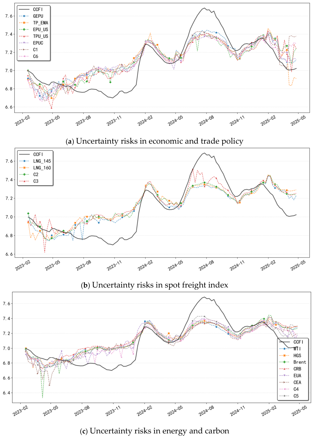
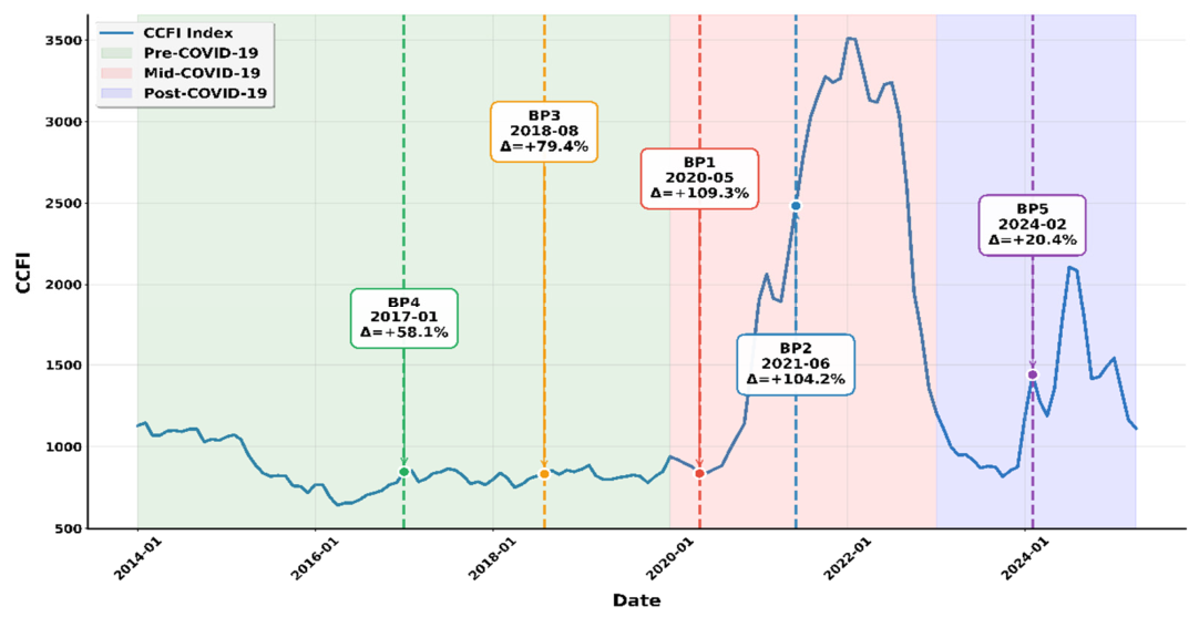
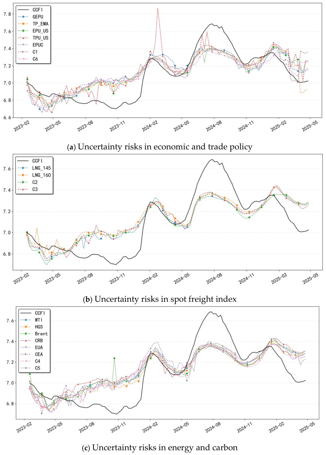
• Three-stage dynamic risk integration: Uncertainty risks are integrated with dynamic event windows through a three-stage experimental protocol. This protocol spans pre-COVID-19, mid-COVID-19, and post-COVID-19 regimes. The framework treats major international events as scenario conditions rather than static dummy variables. This design allows the model to examine how different shock types affect the transmission of uncertainty risks to the CCFI. It also separates the initial event impact from prolonged shock propagation through the Shock Kernel. This approach improves the practical value of the experiments for shipping market monitoring and risk management.

The remainder of this paper is organized as follows. Section 2 reviews related work and identifies research gaps. Section 3 presents the proposed methodology. Section 4 reports experimental results and comparative analyses. Section 5 concludes the paper and outlines future research directions.

2. Related Works

Container freight forecasting is influenced by multiple external drivers, including international trade policy, geopolitical events, energy and carbon markets, and major global events. These factors affect cargo flows, port operations, and overall freight volatility. Accurately capturing these effects is critical for forecasting and risk management. This section reviews prior literature and shows how it motivated the development of the proposed framework.

2.1. External Risk Effects on Container Freight Rates

External risks influence container freight rates through multiple channels. Trade conflicts and sanctions can block shipping routes, disrupt port operations, and force shipping companies to adjust transportation strategies, which in turn affects the distribution of ship capacity and cargo demand [7]. Geopolitical tensions and public health emergencies also create sudden market shocks that alter freight rate volatility and may induce structural changes in indices [8]. Such risks should therefore be treated as dynamic forecasting drivers rather than background context.

Several studies have examined how uncertainty risks shape freight rate dynamics. Yin et al. [9] developed a real-time multi-step forecasting system with a three-stage preprocessing strategy for the containerized freight market, showing the importance of structured preprocessing for freight forecasting, which motivates the use of dynamic event windows. Wu [10] studied climate and geopolitical risks affecting shipping markets across multiple horizons, highlighting the need for multi sources uncertainty indicators. Wang et al. [11] constructed multi-dimensional event databases for the container shipping market and applied feature selection and clustering to identify relevant exogenous signals from complex uncertainty indicators. Khan et al. [8] showed that geopolitical and climate uncertainties affect maritime freight rates conditionally, with transmission strength shifting across market regimes.

Despite these advances, most studies focus on a limited set of indices or specific event types and treat shocks as static inputs. They often ignore overlapping, lagging, or decaying effects of uncertainty shocks. Collectively, these findings confirm that the multi-stage influence of uncertainty on freight rates cannot be captured by static or single-index approaches [12]. They motivate the design of a forecasting framework that explicitly models how risk effects evolve, overlap, and decay over time.

2.2. Shipping Energy

Energy and carbon variables have been recognized as critical factors influencing container shipping costs and freight rate dynamics. Chen et al. [13] examined energy- and carbon-related mechanisms in shipping markets, showing that energy cost pressure and carbon-related uncertainty can affect container shipping cost stability. Emami Javanmard et al. [14] quantified energy conservation and greenhouse gas reduction potentials in the transportation sector through scenario analysis, highlighting the role of environmental factors in cost forecasting. Zhu et al. [15] proposed a robust carbon emission quota allocation mechanism using zero-sum gains data envelopment analysis, illustrating how regulatory frameworks influence cost dynamics. These studies established the foundation for incorporating fuel prices, LNG rates, and carbon emissions as essential inputs for freight index forecasting, as they capture both cost-side pressures and green-transition uncertainty.

Energy and carbon variables exhibit nonstationary seasonal patterns that complicate freight rate forecasting. Seasonal variations in fuel demand, driven by weather conditions and shipping activity cycles, interact with policy-driven carbon pricing mechanisms that adjust periodically. Song et al. [16] demonstrated that ship energy consumption exhibits strong spatiotemporal variability under variable navigation conditions. This reflects the time-dependent nature of the energy–freight relationship. Shi et al. [17] showed that regulatory frameworks introduce temporal variability in compliance costs. Commodities in the energy supply chain experience seasonal demand shifts that propagate to freight markets. These seasonal effects are not fixed: energy price shocks, policy adjustments, and supply disruptions cause seasonal patterns to drift over time, challenging forecasting models that rely on stationary seasonal decomposition.

These studies have established the importance of energy and carbon variables in freight forecasting and revealed their dynamic, time-varying impacts on shipping costs. However, challenges remain in capturing nonstationary seasonal drift and abrupt shock effects in energy–freight relationships. Existing approaches typically assume fixed seasonal structures and lack mechanisms to model evolving patterns or event-driven disruptions. Building upon these insights, the proposed framework extends decomposition-based forecasting to address these gaps. The framework incorporates adaptive mechanisms for time-varying seasonality and external shock effects while preserving model interpretability.

2.3. CCFI Forecasting

CCFI encompasses both spot and forward rates from major Chinese ports and aggregates data from 22 leading shipping companies. This standard parameter offers a robust benchmark for tracking dynamics in China’s containerized export shipping market [18]. Research on CCFI forecasting has gradually evolved from decomposition based and system-based models to nonlinear learning and hybrid deep learning approaches.

Decomposition-based and system-based studies highlighted the importance of separating structural patterns in freight index forecasting. Wu et al. [19] demonstrated that hybrid decomposition combined with probabilistic modeling effectively forecasts highly volatile maritime freight indices. Their approach decomposed the series into frequency components and applied Gaussian process regression, highlighting the value of decomposition-based forecasting for nonstationary shipping data. Kim et al. [20] integrated decomposition with two-stage attention to capture multi-scale freight rate dynamics. Their work confirms that decomposition improves forecast accuracy. Jeon et al. [21] utilized system dynamics to forecast the CCFI, considering market-driven supply and demand factors. These studies demonstrated that CCFI exhibits strong seasonal and trend components, establishing decomposition as a foundational step and motivating the use of Prophet as the decomposition backbone in this study. Regression-based models, however, have limitations, including weak adaptability to external changes and limited responsiveness to sudden events.

Subsequent research introduced nonlinear modeling capabilities. Zeng et al. [22] found that traditional approaches struggle to capture the nonstationary and nonlinear nature of freight rates, and regression models are insufficient for complex price behaviors. The complexity, irregularity, randomness, and nonlinearity of container freight indices challenge conventional prediction methods. This coincided with the rapid development of deep learning, leading to the adoption of neural network forecasting methods [23]. Compared to traditional machine learning, deep learning exhibits strong adaptability and can extract complex relationships from data. Liu et al. [24] demonstrated that deep learning models outperform traditional econometric and machine learning methods on nonstationary freight indices by learning in-depth features directly from data. Wu and Gong [25] demonstrated that deep learning can extract predictive signals from cross-market indicators for freight rate forecasting. These advances support the integration of deep learning components in forecasting frameworks.

More recent hybrid models combine complementary neural components to capture multi-scale temporal patterns. Su et al. [26] showed that combining complementary neural components improves multi-scale feature extraction for container freight forecasting. Wang et al. [27] proposed a multi modal decomposition deep learning framework that integrates uncertainty indices across temporal scales, demonstrating that external event information enhances freight rate forecasts during volatile market condition. Han et al. [28] constructed a hybrid CNN-LSTM model to forecast the relationship between CCFI and financial markets, showing improved predictive accuracy. These hybrid architectures demonstrate that integrating local pattern extraction with long-range dependency modeling yields superior forecasting performance and highlights the need to capture both local fluctuations and global trends. This progression directly informs the design of the Temporal Convolution Kolmogorov-Arnold Network (TCKAN) structure, which combines temporal convolution with Kolmogorov–Arnold networks to model both local fluctuations and global trends, providing a comprehensive solution for multi-stage freight forecasting.

These studies have established strong foundations for freight forecasting through decomposition and deep learning integration. However, three gaps persist in existing research. External shocks are treated as static features rather than evolving events with decaying effects. Seasonal patterns are assumed fixed rather than phase-drifting. Model outputs lack diagnostic parameters for diagnostic use. While prior work demonstrated the effectiveness of decomposition and hybrid neural architecture, challenges remain in modeling time-decaying shock effects, nonstationary seasonal drift, and maintaining interpretability in complex hybrid systems. Building upon these insights, the proposed framework extends decomposition-based forecasting to address these gaps. The framework incorporates adaptive mechanisms for shock decay modeling, time varying seasonality, and sparse interpretable nonlinear transformations while preserving the strengths of prior hybrid approaches.

3. Methodology

To effectively forecast the container shipping market under uncertainty risks, this study proposes a Prophet-Temporal Convolution Kolmogorov-Arnold Network-Warped Fourier and Shock Kerne (Prophet–TCKAN–WFSK) framework. The framework is organized into five stages. These stages correspond to Figure 1:

Stage I: Input. This stage provides historical observations for model training. Multi-source time series data are collected and integrated. These data include CCFI, uncertainty risk features, and major international events.

Stage II: Processing. This stage constructs uncertainty risk features and reduces redundant information. MIC is used to detect nonlinear associations. Boruta evaluates multivariate feature importance. Granger causality verifies lagged temporal predictability. K-shape clustering groups temporally similar exogenous indicators. The cluster centroids are then used as aggregated features.

Stage III: Decomposition. This stage separates structural components from complex residual dynamics. Prophet decomposes the CCFI series into trend, seasonality, event, and residual components. This decomposition provides structured inputs for subsequent residual forecasting.

Stage IV: Residual Prediction. This stage captures the nonlinear dynamics that Prophet cannot fully explain. TCKAN learns nonlinear residual patterns. The Warped Fourier module models seasonal phase drift. The Shock Kernel module captures shock intensity and decay. These modules work together to capture regime-specific patterns and generate the residual forecast.

Stage V: Results and Evaluation. This stage evaluates forecasting performance and cross-regime adaptability. Standard validation experiments assess general predictive accuracy. Dynamic time-window analysis examines how the model responds to pre-COVID-19, mid-COVID-19, and post-COVID-19 regimes. Bai–Perron breakpoints provide post hoc statistical support for regime characterization. They are not used as forecasting components, model inputs, training information, hyperparameter selection criteria, or experimental configuration rules.

Table A1. Functional roles of methodological components in the proposed framework.

Stage	Component	Functional Role	Purpose
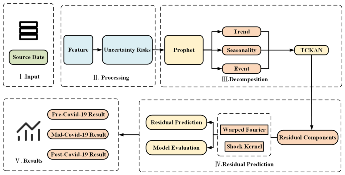
I. Input	Multi-source data collection	Historical data construction	Collect CCFI, uncertainty-risk indicators, and major event information for model training.
II. Processing	MIC	Nonlinear association detection	Identify nonlinear relationships between uncertainty-risk indicators and CCFI.
II. Processing	Boruta	Feature importance evaluation	Select informative predictors through random forest-based importance comparison.
II. Processing	Granger causality	Lagged predictability verification	Verify whether selected variables provide temporal predictive information.
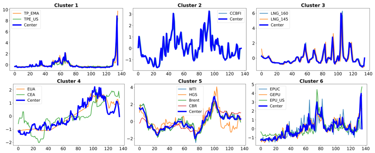
II. Processing	K-shape clustering	Temporal pattern grouping	Group temporally similar exogenous indicators and reduce feature redundancy.
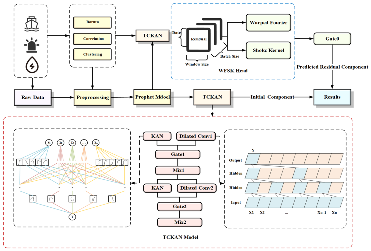
III. Decomposition	Prophet	Structural decomposition	Separate trend, seasonality, event, and residual components from the CCFI series.
IV. Residual Prediction	TCKAN	Nonlinear residual learning	Capture local temporal patterns and nonlinear residual dynamics.
IV. Residual Prediction	Warped Fourier	Seasonal phase-drift modeling	Model nonstationary seasonal phase shifts under regime changes.
IV. Residual Prediction	Shock Kernel	Event-shock decay modeling	Capture event-shock intensity, diffusion, and decay effects.
IV. Residual Prediction	Gating mechanism	Adaptive component fusion	Combine residual, seasonal, and shock components while suppressing noisy information.
V. Results and Evaluation	Bai–Perron test	Structural breakpoint identification	Provide statistically supported breakpoints for regime segmentation and experiment design.
V. Results and Evaluation	Three-stage analysis	Regime-specific evaluation	Assess forecasting behavior across pre-COVID-19, mid-COVID-19, and post-COVID-19 regimes.

in Appendix A summarizes the functional role of each methodological component. This organization clarifies how different methodological choices work together in the forecasting pipeline.

This modeling framework employs a strict two-stage training protocol to prevent information leakage. In Stage III, Prophet parameters are estimated to use only the training set to extract trend, seasonal, and event components. These components are fixed before Stage IV, where the TCKAN-WFSK module learns residual patterns without access to test data. This separation ensures that the residual forecasting model cannot access future values through the decomposition pathway.

Figure 1. Modeling progress.

Figure 1. Modeling progress.

3.1. Uncertainty Risk

Key uncertainties in the container shipping market arise from economic-trade policy risks and energy market dynamics. This study compiles an uncertainty-risk database for the experiment by integrating multiple uncertainty indices. Economic and policy uncertainty indices are sourced from Baker et al. [29]’s framework, Clarkson SIN Database, and iFinD Database. Geopolitical and policy indices are constructed using country-specific newspaper and magazine data and official government sources, while energy-related indices primarily draw from agency announcements. Detailed data source websites and access links for all variables in

Table 1. Uncertainty risks index.

Definition	Labels	Correlation	Lag	p-Value	Category
EU Emissions Trading System Allowance	EUA	0.70	1	0.0581	Carbon market
Commodity Research Bureau	CRB	0.70	1	0.0278	Energy market
China Carbon Emissions Allowance	CEA	0.54	2	0.0833	Carbon market
West Texas Intermediate Crude Oil	WTI	0.51	6	0.0193	Energy market
Brent Crude Oil Benchmark Price	Brent	0.48	5	0.0003	Energy market
Henry Hub Natural Gas Spot Price	HGS	0.45	3	0.0024	Energy market
LNG 145K CBM Spot Rate	LNG-145	0.38	4	0.0795	Spot freight
Equity Market Volatility of Trade Policy	TP-EMA	0.38	4	0.0529	Trade policy
Economic Policy Uncertainty of U. S	EPU-US	0.38	6	0.0099	Economic policy
Global Economic Policy Uncertainty	GEPU	0.33	2	0.0230	Economic policy
China Coastal Bulk Freight Index	CCBFI	0.32	1	0.0160	Spot freight
Economic Policy Uncertainty of China	EPUC	0.31	2	0.0681	Economic policy
LNG 160K CBM Spot Rate	LNG-160	0.31	5	0.0443	Spot freight
Trade Policy Uncertainty of U.S.	TPE-US	0.30	6	0.0054	Trade policy

are provided in

Table A2. Data source websites.

Labels	Website Name	Website URL
CCFI	Clarksons Research	https://www.clarksons.net (accessed on 23 January 2026)
LNG-145	Clarksons Research	https://www.clarksons.net (accessed on 23 January 2026)
LNG-160	Clarksons Research	https://www.clarksons.net (accessed on 23 January 2026)
EPU-US	Economic Policy Uncertainty	https://www.policyuncertainty.com (accessed on 22 January 2026)
EPUC	Economic Policy Uncertainty	https://www.policyuncertainty.com (accessed on 22 January 2026)
GEPU	Economic Policy Uncertainty	https://www.policyuncertainty.com (accessed on 22 January 2026)
TP-EMA	Economic Policy Uncertainty	https://www.policyuncertainty.com (accessed on 22 January 2026)
TPE-US	Economic Policy Uncertainty	https://www.policyuncertainty.com (accessed on 22 January 2026)
EUA	iFinD Database	https://www.51ifind.com (accessed on 18 January 2026)
CRB	iFinD Database	https://www.51ifind.com (accessed on 18 January 2026)
CEA	iFinD Database	https://www.51ifind.com (accessed on 18 January 2026)
WTI	iFinD Database	https://www.51ifind.com (accessed on 19 January 2026)
Brent	iFinD Database	https://www.51ifind.com (accessed on 19 January 2026)
HGS	iFinD Database	https://www.51ifind.com (accessed on 19 January 2026)
CCBFI	iFinD Database	https://www.51ifind.com (accessed on 19 January 2026)

in Appendix B.

Given the extensive feature space, this study uses Maximum Information Coefficient–Boruta (MIC–Boruta) procedure [30,31,32] together with Granger causality testing [33]. MIC–Boruta is used to efficiently select relevant variables, while the Granger predictive information between predictors and target features. Formally, the Maximal Information Coefficient between variables X and Y is defined as

$$I(X;Y)=\iint f(X,Y){log}_2\left({\displaystyle \frac{f(X,Y)}{f\left(X\right)f\left(Y\right)}}\right)dXdY$$

(1)

$$MIC(X,Y)={max}_{\left|X\right|\left|Y\right|<B}{\displaystyle \frac{I(X;Y)}{log\left(min\right(\left|X\right|,\left|Y\right|\left)\right)}}$$

(2)

where $I(X;Y)$ is the mutual information between $X$ and $Y$, $\left|X\right|$ and $\left|Y\right|$ are the number of grid bins, and $B$ is a grid-size constraint with $n$ being the sample size [32].

The Boruta algorithm evaluates feature importance through comparison with shadow features. In each iteration $t$, a set of shadow features $S^{\left(t\right)}$ is created by randomly permuting the original features. A random forest is trained, and the importance of each original feature, $Imp\left(X_j^{\left(t\right)}\right)$, is compared against the maximum importance achieved by any shadow feature, defined as

$$M^{\left(t\right)}={max}_{k}Imp\left(S_k^{\left(t\right)}\right)$$

(3)

where $S_k^{\left(t\right)}$ represents the $k$-th shadow feature at iteration $t$, and ${max}_k$ denotes the maximum value across all shadow features. An original feature scores a hit if $Imp\left(X_j^{\left(t\right)}\right)>M^{\left(t\right)}$. After $T$ iterations, a binomial test is applied to the hit distribution. A feature is formally retained if its hit rate significantly exceeds the expectation of random chance.

Granger causality is tested using the F-statistic:

$$F={\displaystyle \frac{(RS{S}_r-RS{S}_u)/p}{RS{S}_u/(T-2p-1)}}$$

(4)

where $RS{S}_r$ is the restricted residual sum of squares (excluding lagged $X$), $RS{S}_u$ is the unrestricted residual sum of squares (including lagged $X$), $p$ is the lag order, and $T$ is the sample size. A variable $X$ is said to Granger-cause $Y$ if the null hypothesis, or the lagged values of $X$, do not improve the prediction of $Y$, which is rejected at a $p$-value $\le 0.10$. The experimental design explicitly incorporates cyclical lag effects. Table 1 shows uncertainty risks. Variable with p-value ≤ 0.10 exhibits lagged predictive relationships.

This method is designed to preserve nonlinear dependencies. MIC captures arbitrary functional relationships without linearity assumptions. Boruta evaluates multivariate importance through random forests, which naturally capture nonlinear interactions. Granger causality tests directional predictability at a relaxed threshold (p ≤ 0.10). Because nonlinear associations are already validated by MIC and Boruta, the Granger stage verifies temporal precedence without re-testing nonlinearity. This feature selection pipeline is designed to reduce sequential filtering bias by prioritizing retention over aggressive pruning. MIC is used as the first screening step because it captures arbitrary nonlinear associations without imposing a linear functional form. Boruta is then applied as an all-relevant feature selection method based on random forest importance and shadow feature comparison. This step retains variables that show predictive relevance in a multivariate nonlinear setting rather than selecting only a minimal subset. Granger causality testing is used only after these two nonlinear screening steps. Its role is to examine lagged predictive relationships rather than to identify formal causal effects. The relatively relaxed threshold of $p\le 0.10$ is adopted to avoid premature exclusion of variables that may contain delayed predictive information. Therefore, the sequential logic of nonlinear association, multivariate importance, and lagged predictability is designed to preserve informative predictors while reducing redundant inputs.

The K-shape clustering method clusters the time series data [34]. Unlike Euclidean distance-based clustering, K shape preserves the temporal shape of standardized time series by using shape-based distance. For two standardized time series $x$ and $y$, the shape-based distance is defined as

$$SBD(x,y)=1-\underset{\tau }{max}NC{C}_{\tau }(x,y)$$

(5)

where $NC{C}_{\tau }(x,y)$ denotes the normalized cross correlation between $x$ and $y$ under time shift $\tau$. A smaller $SBD(x,y)$ indicates stronger temporal shape similarity.

The clustering objective can be written as

$$\underset{C_1,\dots ,C_K}{min}{\displaystyle \sum _{k=1}^K}\sum _{x_i\in C_k}SBD(x_I;c_k)$$

(6)

where $C_k$ is the $k$-th cluster and $c_k$ is its centroid. The number of clusters is selected using the elbow criterion based on the sum of squared errors:

$$SSE={\displaystyle \sum _{k=1}^K}\sum _{x_i\in C_k}{\parallel x}_i-c_k{\parallel }^2$$

(7)

The resulting centroids are used as aggregated exogenous inputs to reduce redundancy among temporally similar variables.

The optimal number of clusters was dynamically determined as K = 6, with the dark blue line in Figure 2 representing the trend centerline for each cluster. Cluster 1 (C1): trade policy uncertainty; Cluster 2 (C2): dry bulk freight rates; Cluster 3 (C3): spot rates; Cluster 4 (C4): carbon allowance (quota) prices; Cluster 5 (C5): energy prices; Cluster 6 (C6): economic policy uncertainty.

After clustering, we further evaluated multicollinearity among the six cluster centroids using variance inflation factors. The VIF values range from 1.26 to 3.16, all below the commonly used threshold of 5, indicating that the centroid inputs do not exhibit severe multicollinearity. Detailed diagnostic results are reported in

Table A3. Multicollinearity diagnostics for K-shape cluster centroids.

Cluster Centroid	Main Represented Category	VIF
C1	trade policy uncertainty	1.57
C2	dry bulk freight rates	1.29
C3	spot rates	1.26
C4	carbon allowance prices	3.16
C5	energy prices	2.43
C6	economic policy uncertainty	2.88

. This integrated clustering method aggregates temporally similar variables into centroid inputs, serving as an implicit redundancy control step within the feature selection pipeline and helping mitigate multicollinearity among temporally similar variables.

3.2. Prophet-TCKAN-WFSK

The uncertainty risk variables and major international events create multi-dimensional challenges involving seasonal superposition, lag effects, and strong nonlinear interactions [35]. To address these in small-sample, nonstationary forecasting, we introduce the Prophet–TCKAN–WFSK model (Figure 3). This architecture integrates a dual-path gated backbone with a specialized decoupled output mechanism to decode complex dynamics [36]. First, Prophet alleviates the deep learning burden by extracting macro-level trends and principal seasonality, and residual-based prediction attenuates noise and, under appropriate sampling conditions, better aligns with the informational content of the data, thereby improving predictive accuracy in small sample settings [37]. The core feature extraction employs a dual-path gated Temporal Convolutional Kolmogorov–Arnold Network (TCKAN). This backbone fuses a convolutional branch for capturing local temporal patterns [16] with a Kolmogorov–Arnold Network (KAN) branch that models smooth cross-variable nonlinear responses via learnable activation functions [38]. The prediction head incorporates two novel modules: a Warped Fourier module that reparametrizes seasonal phases using B-spline monotonic warping to accommodate nonstationary shifts [39], and a Shock Kernel module that parameterizes interpretable half-life decay for abrupt events [40].

This complementary fusion establishes a robust macro–micro forecasting framework. By offloading global non-stationarity to Prophet, the deep network focuses exclusively on refining complex residuals. The TCKAN backbone mathematically bridges TCN’s local temporal bias with KAN’s nonlinear approximation, effectively separating high-frequency noise from purifiable signals. Crucially, the Warped Fourier (WF) and Shock Kernel (SK) modules exhibit a distinct internal synergy: WF dynamically corrects continuous seasonal phase shifts via monotonic warping, while SK explicitly captures discreet, aperiodic exogenous impulses. This decoupling ensures that transient shocks do not distort the learning of evolving seasonal patterns. These components integrate into a holistic system where the TCKAN backbone extracts high-fidelity features that are decoded by the WFSK head and finally fused via a gating mechanism. Constrained by warp smoothness and gate entropy regularization, this joint optimization minimizes overfitting in small-sample regimes, yielding stable point forecasts with improved robustness and diagnostic transparency.

Although this study primarily emphasizes small-sample robustness, the framework has a computationally feasible structure under the tested short window setting. Prophet decomposition scales linearly with the number of observations [41], suggesting compatibility with both weekly and potentially higher-frequency data without major changes to the algorithmic structure [42]. The TCKAN backbone’s dual-path design maintains this linear scaling: temporal convolutions operate on fixed-size local windows [43], and KAN activation dimensions are independent of sequence length [44]. For fixed window size, channel dimension, and spline basis size, the dominant forecasting computation grows approximately in proportion to the number of time steps [43], supporting training and inference feasibility under controlled settings.

Above all, unlike conventional hybrid architectures, which stack components in a serial pipeline to enhance representation capacity, the proposed framework adopts modular hybrid architecture [43]. Prophet first separates global non-stationarity from residual dynamics. The TCKAN backbone then processes residuals through two parallel branches that fuse local convolutional encoding with Kolmogorov–Arnold function approximation. The WFSK head finally decouples continuous seasonal drift from discrete event shocks. This three-level decoupling addresses small-sample, multi-regime forecasting through structural specialization rather than depth or width expansion and constitutes the core methodological novelty and theoretical motivation of the framework [33].

3.2.1. Prophet

Prophet is an open-source automated time series prediction model released by the Facebook team. The model can show excellent and robust prediction performance in situations that contain complex anomalous features [45]. Various hybrid Prophet models have demonstrated significant advantages over traditional machine learning methods in time series data forecasting [39]. Prophet is selected over common adaptive decomposition methods for three reasons. First, it produces a semantically structured decomposition into trend, seasonality, and event terms, whereas adaptive methods yield frequency-layered modes without separating recurring seasonality from event-driven anomalies. Second, it is relatively robust to missing values and outliers through its additive modeling structure and trend-change regularization, which is critical for shipping data subject to operational disruptions. Third, its additive decomposition avoids the boundary effects that arise when adaptive methods are reapplied during rolling forecasts [41,46]. In this study, Prophet decomposes the data into trend, seasonal, event, and residual components, thereby establishing a decomposition basis for subsequent residual forecasting. Prophet parameters are estimated using only the training set to extract trend, seasonal, and event components and remain fixed during subsequent residual forecasting, preventing information leakage from test data. The specific procedure is as follows:

For the target series ${\left\{y_t\right\}}_{t=1}^T$ and the selected exogenous uncertainty vector $x_t\in {\mathbb{R}}^{d_z}$, Prophet decomposes the original CCFI series into trend $T_t$, seasonality $S_t$, event term $H_t$, and residual component $r_t$. Here, $d_z$ denotes the number of selected exogenous uncertainty indicators.

$$y_t=T_t+S_t+H_t+r_t$$

(8)

The structural components $T_t$, $S_t$, and $H_t$ capture the additive patterns that Prophet can explain. The residual component $r_t$ contains the remaining dynamics that cannot be captured by additive decomposition. These dynamics include autoregressive residual patterns, nonlinear responses to exogenous uncertainty indicators, and lagged responses to external shocks.

The shock intensity $e_t$ is produced by a compact event encoder. The encoder takes the event increment window ${\Delta }_t$ as input:

$$e_t=f_{enc}\left({\Delta }_t\right)\ge 0.$$

(9)

The event increment window is defined as

$${\Delta }_t=\left[{\delta }_t,{\delta }_{t-1},\dots ,{\delta }_{t-H}\right]$$

(10)

where $H$ denotes the length of the event history window. The vector ${\delta }_t$ contains the observed event-related shock indicators at time $t$. The encoder $f_{enc}$ is implemented as a multi-layer perception with GELU hidden activation and a Softplus output. The Softplus output ensures that $e_t$ is nonnegative. The resulting $e_t$ provides the TCKAN module with information about the magnitude and recency of external shocks.

We then construct the structured residual input vector $X_t$ for the TCKAN module. The vector combines residual lags, lagged exogenous uncertainty variables, and the shock intensity term $e_t$:

$$X_t=\left[r_{t-i_r},\hspace{0.17em}{x}_{t-i_1}^{\left(1\right)},\hspace{0.17em}{x}_{t-i_2}^{\left(2\right)},\hspace{0.17em}\dots ,\hspace{0.17em}{x}_{t-i_n}^{\left(n\right)},\hspace{0.17em}{e}_t\right]$$

(11)

Here, $i_r$ denotes the residual lag. The term $i_n$ denotes the lag assigned to the $n$-th exogenous uncertainty variable. These lags are determined from the Granger causality results reported in Table 1. This construction ensures that the TCKAN module learns residual dynamics from three sources: residual history, lagged exogenous uncertainty information, and observed shock intensity.

The construction of $X_t$ follows a rigorous logic. Prophet decomposes the series into trend, seasonal, event, and residual components. The trend, seasonal, and event terms capture structural patterns that are well described by additive decomposition. The residual $r_t$ contains the dynamics that the additive model cannot explain. These dynamics include two types of effects. First, nonlinear interactions among uncertainty drivers. Second, the lagged response of freight rates to external shocks. The TCKAN module is therefore tasked with predicting $r_t$ using three sources of information: (i) the residual’s own past values $r_{t-i}$, which capture autoregressive dynamics; (ii) lagged exogenous uncertainty indicators $x_{t-i_n}^{\left(n\right)}$, which supply external drivers of residual variation; and (iii) the shock intensity $e_t$, which informs the module of the magnitude and recency of structural breaks. The lags $i_r$ and $i_n$ are specified in Table 1 and reflect the empirically determined lead times at which each variable Granger-causes CCFI fluctuations.

3.2.2. TCKAN

In Figure 3, TCKAN runs KAN and Temporal Convolutions in parallel and fuses their outputs via a gating mechanism. Dilated convolution uses an adjustable dilation factor to expand the receptive field while remaining causal (depending only on current and past inputs) to capture long-range dependencies [47]. KAN is a neural network structure based on the Kolmogorov–Arnold representation theorem. KAN places learnable activation functions on network edges so each connection learns both a weight and an adaptive nonlinear transform, substantially enhancing modeling of complex nonlinear relationships [48]. Parallel complementarity maintains expressiveness, reduces parameter redundancy and small sample overfitting, and improves diagnostic transparency. Additionally, the gating mechanism is particularly suited to the small-sample regime: it operates through elementwise selection with a parameter count that grows linearly with the number of channels, keeping model capacity proportional to the available data. Attention-based fusion, by contrast, can introduce higher computational and memory costs due to pairwise interaction modeling, especially for longer sequences. Therefore, attention-based fusion is deferred to future work on larger datasets [49]. The use of KAN instead of a Transformer-based architecture is motivated by the data scale and the residual learning objective of this study. Transformer-based models are powerful for long sequences and large-scale multivariate settings, but their attention layers can introduce additional parameters and pairwise interaction costs. In contrast, the present framework first removes global trend, seasonality, and event components through Prophet. The remaining task is to learn nonlinear residual mappings under limited weekly observations. KAN is well suited to this setting because its learnable spline activations provide flexible univariate nonlinear transformations with controllable capacity. This design supports nonlinear approximation under small-sample conditions and enables sparsity-based diagnostic analysis of the learned activation functions. Therefore, KAN is selected not as a universal replacement for Transformer architectures, but as a better aligned component for residual nonlinear learning in the proposed decomposition-based framework [47]. The TCKAN process is as follows:

The TCKAN backbone comprises stacked hybrid blocks that take $X_t$ as input. For the $l$-th layer, the input is $h_{l-1}\in {\mathbb{R}}^{B\times W\times C_{l-1}}$. Here, $B$ is the batch size, $W$ is the window size, and $C_{l-1}$ is the number of input channels.

The convolutional branch captures local temporal patterns

$$c_l={Conv}_l\left(h_{l-1}\right)$$

(12)

The KAN branch captures nonlinear transformations through learnable B-spline activation functions:

$$k_l={KAN}_l\left(h_{l-1}\right)$$

(13)

The two branch outputs are fused through a gating unit:

$$g_l=\sigma \left(W_l^{\left(g\right)}·c_l\right)$$

(14)

$$m_l=g_l\odot c_l+\left(1-g_l\right)\odot k_l$$

(15)

$$h_l=m_l+R_l\left(h_{l-1}\right)$$

(16)

where $c_l$ denotes the convolutional branch output. $k_l$ denotes the KAN branch output. $\sigma \left(\cdot \right)$ denotes the sigmoid activation function. $W_l^{\left(g\right)}$ and $b_l^{\left(g\right)}$ are learnable gating parameters. The symbol $\odot$ denotes elementwise multiplication. The mapping $R_l\left(\cdot \right)$ is a $1\times 1$ convolution used for dimensional alignment. The final hidden state $h_T$ is obtained from the last time step and is passed to the WFSK head.

3.2.3. Warped Fourier

TCKAN generates a unified temporal encoding to mitigate phase drift from external uncertainties and major events. Using a monotonically learnable warp function $g\left(\tau \right)$, we remap the original time ${\tau }_t$ into a stabilized phase domain. At the same time the unconstrained warping function $g\left(\tau \right)$ is prone to forming indeterminate structures, which may result in high-frequency oscillations that fit observational noise. $L_{\mathit{warp}}$ serves as a discrete approximation to curvature penalization, suppressing abrupt changes in the derivatives of $g\left(\tau \right)$. As defined below,

$${\tau }_t={\displaystyle \frac{t-1}{n-1}}, 0<g\left({\tau }_1\right)<g\left({\tau }_2\right)<\cdots <g\left({\tau }_n\right)=1$$

(17)

$$L_{\mathit{warp}}={\displaystyle \frac{1}{n-2}}{\displaystyle \sum _{t=2}^{n-1}}(g\left({\tau }_{t+1}\right)-2g\left({\tau }_t\right)+g\left({\tau }_{t-1}\right){)}^2$$

(18)

where ${\tau }_t$ is normalized time; $g\left(\cdot \right)$ denotes learned monotonic warp; and $n=T$. Notably, $t$ denotes the current time step. Like KAN, $g\left({\tau }_t\right)$ is a smooth, monotone time-warping function constructed by integrating and normalizing a positive B-spline expansion of its derivative in normalized time. It parsimoniously realigns nonuniform seasonal phase. enabling downstream low-rank Fourier and Shock Kernels to more efficiently and robustly capture true periodic and event dynamics, especially under small-sample, nonstationary conditions.

The warp function $g\left(\tau \right)$ has three useful mathematical properties. First, monotonicity is ensured by constructing $g\left(\tau \right)$ through integration of a positive B-spline expansion:

$$g^{\prime }\left(\tau \right)={\sum }_j\mathit{softplus}\left(w_j\right)\cdot B_j\left(\tau \right)$$

(19)

where $B_j\left(\tau \right)\ge 0$ are B-spline basis functions and ${\sum }_j\mathit{softplus}\left(w_j\right)\cdot B_j>0$ for all $j$. Since $g^{\prime }\left(\tau \right)>0$ for all $\tau \in (0,1)$, $g\left(\tau \right)$ is strictly monotone increasing, $w_j$ denotes learnable spline coefficients. Second, identifiability is guaranteed by the normalization constraints $g\left(0\right)=0$ and $g\left(1\right)=1$, which eliminate scale ambiguity. The linear independence of B-spline basis functions ensures that the coefficients $w_j$ are endogenously determined under these constraints. Third, convergence follows from B-spline approximation theory: for any continuous monotone function, there exists a B-spline sequence that converges uniformly as the number of basis functions increases. The curvature regularization term $L_{\mathrm{warp}}$ in Equation (18) further stabilizes convergence by penalizing excessive oscillations in $g^{″}\left(\tau \right)$.

To model the deformation phase across multiple frequencies with a minimal set of parameters, a finite basis is constructed, and low-rank parameterization is employed. The specific implementation is as follows: A set of sinusoidal basis functions is defined in Equations (20) and (21); the final seasonal term ${\mathcal{S}}_t$ is defined in Equation (22):

$$B_f^{sin}\left({\tau }_t\right)=sin\left(2\pi f\hspace{0.17em}g\left({\tau }_t\right)\right)$$

(20)

$$B_f^{cos}\left({\tau }_t\right)=cos\left(2\pi f\hspace{0.17em}g\left({\tau }_t\right)\right)$$

(21)

$${\mathcal{S}}_t={\displaystyle \sum _{j=1}^J}{\theta }_{F,j}{B}_j\left({\tau }_t\right)$$

(22)

For each frequency $f$ in set $F$, sin function basis $B_f^{sin}\left({\tau }_t\right)$ and cos basis functions $B_f^{cos}\left({\tau }_t\right)$ are defined as warping transformations; $F$ denotes the set of frequencies specified by the model. To better account for lag effects, the cardinality of $F$ is set equal to the lag coefficient $i$. Accordingly, the total number of basis functions is set to $J=2\left|F\right|$, and the frequency weight vector ${\theta }_F=U\left(V{h}_T\right)$ is constructed, where $U$ and $V$ are low-rank structure matrices determined by model parameters, and $h_T$ is the information summary generated by TCKAN. $B_j$ refers to the $j$-th mapping after warping transformation. This completes the seasonal term ${\widehat{S}}_t$ for time ${\tau }_t$.

3.2.4. Shock Kernel

Similarly, we consider multivariate interactions and shocks triggered by sudden events and propose a hybrid Shock Kernel that simulates both fast-decaying and slow-decaying shocks to better accommodate heterogeneous shock types. Each kernel is formed as a weighted combination of an exponential decay kernel and a Gaussian diffusion kernel, yielding the result $K$. These increments are processed through number of $\mathrm{k}$ Shock Kernels to obtain $K_k\left({\Delta }_t\right)$. The exponential component is governed by a decay rate ${\lambda }_k$, from which the half-life $t_{1/2,k}$ is derived; the Gaussian diffusion component is controlled by the parameter ${\sigma }_k$. The Shock Kernels need project shock intensities $e_t$ across multiple event windows. Concretely, over several temporal horizons, Prophet’s changepoint and event terms are aligned with the event increment windows ${\Delta }_t$, causing each window to generate a shock increment ${\delta }_t$. The Shock Kernel first encodes the event increment window via an encoder operation $f_{enc}\left({\Delta }_t\right)$ and then maps $e_t$ onto multiple event increment windows. The resulting filtered outputs are then jointly aggregated into the final composite shock term ${\widehat{S}}_t$, explicitly capturing the lagged and compounding effects of historical shocks.

$$K_k\left({\Delta }_t\right)={\alpha }_k{e}^{-{\lambda }_k{\Delta }_t}+(1-{\alpha }_k)e^{-{\left({\Delta }_t/{\sigma }_k\right)}^2}$$

(23)

$$t_{1/2,k}={\displaystyle \frac{ln2}{{\lambda }_k}}$$

(24)

$${\widehat{S}}_t=e_t{\displaystyle \sum _{k=1}^K}{\theta }_{S,k}\left(h_T\right)\left({\displaystyle \sum _{{\Delta }_t=0}^H}{K}_k\left({\Delta }_t\right)\right)$$

(25)

Here, $H$ denotes the length of the event history window. $K$ denotes the number of Shock Kernels. The term ${\theta }_{S,k}\left(h_T\right)$ denotes the conditional weight assigned to the $k$-th Shock Kernel. It is generated from the final TCKAN hidden state $h_T$ through a learnable mapping. This design allows the WFSK head to assign different importance to different Shock Kernels according to the current temporal representation. The parameter ${\alpha }_k$ is a learnable adaptive weighting parameter. It dynamically regulates the balance between immediate exponential dissipation and delayed Gaussian propagation for each shock type $k$.

The Shock Kernel distinguishes disruption duration through the learned decay profile. A short-lived disruption is represented by a large exponential decay rate, a short half-life, and a narrow diffusion scale. In this case, the shock term decreases quickly after the event window. A more persistent disruption is represented by a smaller decay rate, a longer half-life, a broader diffusion scale, and repeated non-zero shock weights across adjacent event windows. This allows the module to model longer propagation effects. However, the Shock Kernel is not used as a formal regime-switching classifier or as a structural break detector. Long-term regime changes are handled jointly by Prophet decomposition, Warped Fourier phase adjustment, and the residual learner. The Shock Kernel therefore distinguishes short-lived and persistent shock responses at the forecasting-mechanism level, rather than assigning causal regime labels.

A perceptual gated network is used to process the model’s information summary component through a gating operation ${\widehat{R}}_t$, which is then integrated with the seasonal term and shock term to produce a unified output representing the predictive residual ${\widehat{r}}_t$. The forecast parameters are subsequently combined with the initial decomposition terms to arrive at the final prediction ${\widehat{y}}_t$.

$${\widehat{R}}_t=w_r^{\top }{h}_T+b_r$$

(26)

$${\widehat{r}}_t={\alpha }_1{\widehat{R}}_t+{\alpha }_2{\mathcal{S}}_t+{\alpha }_3{\widehat{S}}_t$$

(27)

$${\widehat{y}}_t=T_t+S_t+H_t+{\widehat{r}}_t$$

(28)

Here, $w_r$ and $b_r$ are learnable parameters for the residual projection. The coefficients ${\alpha }_1$, ${\alpha }_2$, and ${\alpha }_3$ are probability weights assigned to the residual projection, the Warped Fourier seasonal term, and the Shock Kernel term, respectively. These weights sum to one. The gate coefficients $\alpha =[{\alpha }_1,{\alpha }_2,{\alpha }_3]$ are produced by

$$\alpha =\mathit{softmax}\left({\displaystyle \frac{W_g{h}_T}{p}}\right)$$

(29)

where $W_g$ is the learnable weight matrix. The parameter $p$ is a temperature parameter that is progressively reduced during training. Higher $p$ yields softer mixing of the three components during early training. Lower $p$ enforces sharper routing as training progresses. The gate coefficients satisfy ${\alpha }_i\ge 0$ and ${\sum }_{i=1}^3{\alpha }_i=1$. The matrix $W_g$ is learned by back propagation together with the TCKAN backbone and the WFSK head.

3.3. Evaluation Metrics and Statistical Tests

To support the evaluation stage in Figure 1, this study uses error metrics and statistical tests to assess forecasting performance. Model accuracy is evaluated using Mean Squared Error (MSE), Mean Absolute Error (MAE), Root Mean Square Error (RMSE), and the coefficient of determination (R²):

$$MSE={\displaystyle \frac{1}{N}}{\displaystyle \sum _{t=1}^N}{(y_t-{\widehat{y}}_t)}^2$$

(30)

$$MAE={\displaystyle \frac{1}{N}}{\displaystyle \sum _{t=1}^N}\left|y_t-{\widehat{y}}_t\right|$$

(31)

$$RMSE=\sqrt{{\displaystyle \frac{1}{N}}{\displaystyle \sum _{t=1}^N}{(y_t-{\widehat{y}}_t)}^2}$$

(32)

$$R^2=1-{\displaystyle \frac{{\displaystyle {\sum }_{t=1}^N}{(y_t-{\widehat{y}}_t)}^2}{{\displaystyle {\sum }_{t=1}^N}{(y_t-\stackrel{-}{y})}^2}}$$

(33)

where $y_t$ denotes the observed value, ${\widehat{y}}_t$ denotes the predicted value, $\stackrel{-}{y}$ denotes the sample mean of the observed values, and $N$ denotes the number of test observations.

Pairwise forecasting performance is evaluated using the Diebold–Mariano (DM) test. For two competing models, the loss differential is defined as

$$d_t=L\left(e_{1,t}\right)-L\left(e_{2,t}\right)$$

(34)

where $e_{1,t}$ and $e_{2,t}$ denote the forecast errors of the two models, and $L\left(\cdot \right)$ denotes the loss function. The DM statistic is calculated as

$$DM={\displaystyle \frac{\stackrel{-}{d}}{\sqrt{\widehat{Var}\left(\stackrel{-}{d}\right)}}}$$

(35)

where $\stackrel{-}{d}$ is the mean loss differential and $\widehat{Var}\left(\stackrel{-}{d}\right)$ is its estimated variance. The resulting p values are adjusted using the Holm–Bonferroni procedure to control for multiple pairwise comparisons.

To provide nonparametric validation, model rankings are further evaluated using the Friedman test. The Friedman statistic is defined as

$${\chi }_F^2={\displaystyle \frac{12N}{K(K+1)}}{\displaystyle \sum _{j=1}^K}{(R_j-{\displaystyle \frac{K+1}{2}})}^2$$

(36)

where $N$ denotes the number of comparable experimental settings, $K$ denotes the number of models, and $R_j$ denotes the average rank of the $j$-th model. When the Friedman test indicates significant overall rank differences, the Nemenyi post hoc critical difference is calculated as

$$CD=q_{\alpha }\sqrt{{\displaystyle \frac{K(K+1)}{6N}}}$$

(37)

where $q_{\alpha }$ is the critical value at significance level $\alpha$. These tests complement the DM tests by providing rank-based statistical evidence across comparable experimental settings.

4. Experiments

4.1. CCFI Dataset and Structural Breakpoints

This study uses weekly CCFI data (January 2014–May 2025), with Figure 4 illustrating its key trends and fluctuations. The Bai–Perron test [50] was applied and identified five major structural breakpoints: January 2017, August 2018, May 2020, June 2021, and February 2024, as shown in Figure 4. All tests are statistically significant at the 5% level, and the 95% confidence intervals for all breakpoints exclude zero. The vertical axis represents the dimensionless CCFI values, while the horizontal axis denotes time. The breakpoints are labeled in order of magnitude of change as BP1 to BP5. BP1 represents the most significant structural breakpoint, corresponding to the highest percentage change, which indicates a major shift in the container shipping market. BP1 and BP2 exhibit the most pronounced structural changes (∆), indicating that the CCFI during this period was strongly impacted by uncertainty risks. Related major international events are shown in

Table 2. Major international events.

Pre-COVID-19		Mid-COVID-19		Post-COVID-19
2014.3–2017.1	International oil price collapse	2020.5– 2021.6	COVID-19 outbreak	2022.12–2023.1	Global geopolitical conflicts
2017.1–2018.8	Brexit, U.S. and European elections	2021.6–2022.10	Omicron variant outbreak	2023.1– 2023.2	Cost-of-living crisis
2018.8–2019.11	China-U.S. trade war	2022.10–2022.12	COVID-19 eased	2023.2– 2023.3	U.S. fed policy

. The Bai–Perron test is conducted as a post hoc characterization of the full historical CCFI series. Its purpose is to validate that the externally chosen COVID-19 segmentation date (May 2020) coincides with a statistically significant regime shift in the data. The test output is not used to inform model training, hyperparameter selection, or experimental configuration at any stage of the analysis.

Specifically, the international oil price collapse from 2014 to 2017 and the Brexit, U.S. and European election period from 2017 to 2018 generated early external shocks. The China–U.S. trade war, which started in 2018, further increased market volatility. The COVID-19 outbreak in 2020 became a major turning point. Global lockdowns and supply chain congestion pushed the CCFI upward. The Omicron outbreak and repeated pandemic disruptions in 2021 and 2022 further strengthened these pressures and helped drive the index to a historical peak. As COVID-19 eased in late 2022, the CCFI declined sharply. Before the fixed test period, global geopolitical conflicts, the cost-of-living crisis, and U.S. Fed policy introduced new external shocks. These events provide the stage-specific event terms used in the dynamic time window analysis. Events after the fixed test boundary are not used to construct training event terms.

The figure spans from January 2014 to May 2025, with the COVID-19 pandemic serving as a key dividing point. This allows us to analyze the impact of uncertainty risks on the CCFI across three distinct periods: pre-pandemic, mid-pandemic, and post-pandemic. By examining these intervals, we can assess the relative importance of uncertainty risks in relation to the CCFI. Structurally, all datasets employed in this study are formatted as point-based multivariate time series. Although the CCFI reflects freight dynamics across geographically distributed shipping routes, the data is aggregated and recorded as discrete scalar observations at weekly intervals. Our variables, including the target CCFI and exogenous drivers, are strictly aligned along the temporal dimension to facilitate sequence modeling. Methodologically, for long-term events, including China–U.S. trade wars, COVID-19, and global geopolitical conflicts, only the first three months with the most pronounced impact are marked as event nodes in Prophet, due to its handling of events and holidays. This threshold is supported by the ablation experiments reported in Appendix C 

Table A4. Event window ablation study results.

Window Length	MAE	RMSE
2 months	0.2314 ± 0.0192	0.3018 ± 0.0196
3 months	0.1978 ± 0.0153	0.2598 ± 0.0169
4 months	0.2204 ± 0.0177	0.2875 ± 0.0186

, where the three-month window achieves the lowest errors. Shorter windows (1–2 months) fail to capture the full propagation of shocks through supply chains, while longer windows risk overfitting to seasonal or trend variations unrelated to the event [45]. This strategy helps prevent overfitting. The prolonged effects are then modeled by the Shock Kernel in our approach.

COVID-19 is used as the principal regime segmentation point because it is an exogenous and economically interpretable event known before model construction. A fully data-driven multi-regime design based on full sample breakpoints is not adopted because it could introduce retrospective information into earlier period model configuration and increase the risk of look-ahead bias. It would also shorten the already limited weekly samples within each regime. Therefore, Bai–Perron breakpoints are used only as post hoc statistical support for regime characterization, not as model inputs, training information, or experimental configuration rules. Other major shocks are still represented through event windows and the Shock Kernel rather than being treated as separate regime boundaries. And to test whether Bai–Perron breakpoints improve forecasting performance when used as event information, we conducted an additional breakpoint-informed robustness experiment. The data split, model architecture, hyperparameters, and training protocol are kept unchanged. Only the event setting is modified. As shown in

Table A5. Breakpoint-informed event setting robustness test.

Event Setting	MAE	RMSE
Proposed event setting without Bai–Perron event nodes	0.2112 ± 0.0509	0.2785 ± 0.0670
COVID Event Window Only	0.2147 ± 0.0515	0.2818 ± 0.0680
COVID and Bai–Perron Event Nodes	0.2133 ± 0.0514	0.2810 ± 0.0678
Bai–Perron Breakpoints as Prophet Event Nodes	0.2228 ± 0.0526	0.2875 ± 0.0694

, adding Bai–Perron event nodes to the COVID-19 event window produces only a small change in MAE and RMSE. Directly treating Bai–Perron breakpoints as Prophet event nodes increases the forecasting errors. These results indicate that Bai–Perron breakpoints do not provide a stable or material forecasting improvement in this setting. Therefore, the Bai–Perron test is retained as post hoc statistical support for regime characterization. It is not used as model input, training information, hyperparameter selection criterion, or experimental configuration rule.

4.2. Hyperparameter Settings

Hyperparameter optimization was performed using random search [51].

Table 3. Parameters.

Parameters	Value	Parameters	Value
Window_size	5	Learning rate	5 × 10−4
Batch_size	4	Changepoint_prior_scale	0.5
Epochs	150	Changepoint_range	0.8
Num_channels	[24, 32]	Holidays_prior_scale	10

presents the optimal baseline hyperparameters for the Prophet-TCKAN-WFSK model determined through this process. Note that while these fixed hyperparameters govern the model architecture and training strategy, the remaining internal parameters are adaptively learned during the training phase.

To ensure reproducibility, a fixed random seed is used across all stochastic operations. Random search is conducted solely during hyperparameter exploration; once the configuration yielding the lowest validation RMSE is selected, the seed is fixed and model training is then conducted under fixed random seeds to minimize stochastic variation.

The parameter choices in Table 3 reflect both domain-specific considerations and small-sample forecasting constraints. Prophet-specific hyperparameters (changepoint_prior_scale, changepoint_range, holidays_prior_scale) are configured following standard Prophet application practices [39], where changepoint_prior_scale controls trend flexibility, changepoint_range determines the proportion of the time series where changepoints are allowed, and holidays_prior_scale adjusts the strength of holiday effects. Deep learning hyperparameters (window_size, batch_size, learning rate, num_channels, Epochs) are selected considering small-sample forecasting constraints [52]. The window size of 5 captures short-term dependencies without overfitting in limited data regimes. The small batch size of 4 is appropriate for the dataset scale and helps regularize training. The learning rate of 5 × 10⁻⁴ balances convergence speed and stability. The num_channels provide sufficient representational capacity while avoiding overparameterization. The epoch count of 150 allows convergence while early stopping based on validation performance prevents overfitting. Final hyperparameter values were determined through random search [51] over candidate ranges, with the configuration yielding the lowest validation RMSE selected for all reported experiments.

4.3. Validation Experiments

To assess the prediction accuracy and robustness of the Prophet-TCKAN-WFSK model under uncertainty risks, we conducted comparative experiments using the following models: TimesNet [53], Autoformer [54], TimeMixer [55], Autoregressive Integrated Moving Average with Generalized Autoregressive Conditional Heteroskedasticity errors (ARIMA–GARCH) [56], Seasonal Autoregressive Integrated Moving Average (SARIMA) [57], and Trigonometric Box–Cox ARMA Trend Seasonal (TBATS) [56]. Autoformer, TimeMixer, and TimesNet are state-of-the-art time series forecasting methods. These selections represent the primary methodological families in time series forecasting, covering econometric, frequency-domain, and attention-based approaches, and their inclusion ensures a more comprehensive comparative experiment.

To ensure rigorous evaluation, we implemented a comprehensive validation protocol for the standard forecasting experiments in Section 4.3.1, Section 4.3.2, Section 4.3.3, Section 4.3.4 and Section 4.3.5. These experiments use chronological 70% training, 10% validation, and 20% testing split to assess general predictive performance under comparable data conditions. Model performance is evaluated using the metrics and statistical tests defined in Section 3.3. MSE, MAE, RMSE, and R² are used to measure forecasting accuracy and goodness of fit. MAE and RMSE values are reported with 95% confidence intervals. Pairwise statistical significance is evaluated using the Diebold–Mariano test with Holm–Bonferroni correction. Friedman nonparametric tests and Nemenyi post hoc tests are further used for comparable model ranking settings. Their results are reported in the notes of the relevant performance tables to avoid redundant tables.

The validation experiments in Section 4.3 serve two purposes. Section 4.3.1, Section 4.3.2, Section 4.3.3, Section 4.3.4 and Section 4.3.5 follow the standard evaluation protocol commonly used in deep learning forecasting studies. They assess the general predictive accuracy, robustness, and component contribution of the proposed framework under comparable data conditions. Section 4.3.6 further examines cross-regime generalization by training the model on pre-COVID-19 data and testing it on the COVID-19-period regime without retraining. This design separates conventional forecasting validation from structural break-oriented evaluation.

4.3.1. Without Exogenous Uncertainty Features

This experiment addresses a question central to the framework’s structural validity: how does the model perform when external uncertainty risk indicators and event-related exogenous features are entirely excluded? By removing all uncertainty risk variables, the experiment isolates the endogenous predictive capacity of the Prophet-TCKAN-WFSK architecture. The model must rely solely on the internal time series structure of trend and seasonality and learn residual dynamics without access to any external shock signals.

This setting also provides a conservative stress test for external variable unavailability. If an important external indicator becomes unavailable or its reporting methodology changes, the affected variable may become unreliable for forecasting. In such cases, the model can be operated without external uncertainty inputs rather than relying on inconsistent indicators. By removing all uncertainty risk variables and event-related exogenous features, this experiment represents a stronger perturbation than the loss of a single indicator. The results in

Table 4. Comparisons without uncertainty features.

Model	MAE	RMSE	DM
Prophet-TCKAN-WFSK	0.1968 ± 0.0182	0.2792 ± 0.0181
TimesNet	0.1862 ± 0.0198	0.2849 ± 0.0185	0.3186
Autoformer	0.2868 ± 0.0431	0.5512 ± 0.0357	−2.1327 **
TimeMixer	0.2046 ± 0.0216	0.3121 ± 0.0202	−0.4822
SARIMA	0.3720 ± 0.0396	0.5704 ± 0.0370	−4.7728 ***
ARIMA-GARCH	0.3602 ± 0.0336	0.5496 ± 0.0356	−4.3482 ***
TBATS	0.3572 ± 0.0327	0.5046 ± 0.0327	−6.3456 ***

Note: Holm–Bonferroni corrected DM test significance levels are denoted by *** $p<0.01$, ** $p<0.05$.

show that the proposed framework maintains stable forecasting performance based on endogenous CCFI structure alone. This does not imply that reporting changes have no impact. It indicates that the framework has a viable fallback configuration when external variables are unavailable or unreliable.

As reported in Table 4, the proposed framework achieves an RMSE of 0.2792 under this constrained setting. This value is lower than the RMSE of TimesNet and TimeMixer, although the DM tests against these two deep learning baselines are not statistically significant. The DM results show significant differences against Autoformer and the econometric baselines, including SARIMA, ARIMA-GARCH, and TBATS. Therefore, the results should be interpreted as evidence of competitive and stable forecasting performance, rather than universal statistical superiority. These findings establish the architecture’s intrinsic robustness: the Warped Fourier component captures dynamic periodicities beyond rigid seasonal assumptions, and the Prophet-TCKAN synergy resolves complex temporal dependencies more effectively than competing frameworks, all without reliance on external uncertainty signals.

4.3.2. With Exogenous Uncertainty Features

Experiments with exogenous uncertainty features are conducted to validate the role of uncertainty risks in CCFI forecasting. These experiments examine whether the Prophet-TCKAN-WFSK model captures uncertainty-driven fluctuations. They also test whether the WFSK module improves adaptability to structural breaks and risk clustering periods. Finally, they evaluate whether the integrated framework captures both trend-related effects and local global temporal patterns.

Four representative uncertainty indicators are selected as structural probes, one from each of the four uncertainty dimensions identified in Table 1. WTI and LNG_160 capture energy cost volatility, TP_EMA captures trade policy uncertainty, and EUA captures carbon pricing pressure. This design spans the principal dimensions relevant to CCFI fluctuations while avoiding redundant comparisons across dimension-internal variables, which would duplicate findings without adding analytical value. The objective is not to evaluate every candidate variable. It is to verify that the framework performs consistently across distinct uncertainty types.

From

Table 5. Comparisons with uncertainty features.

Feature	Model	MAE	RMSE	DM
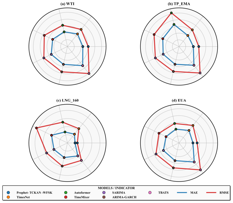
WTI	Prophet-TCKAN-WFSK	0.2248 ± 0.0187	0.3038 ± 0.0197
	TimesNet	0.2353 ± 0.0200	0.3206 ± 0.0208	−0.6239
	Autoformer	0.2205 ± 0.0212	0.3197 ± 0.0207	−0.0231
	TimeMixer	0.2411 ± 0.0265	0.3765 ± 0.0244	−0.7967
	SARIMA	0.2635 ± 0.0256	0.3839 ± 0.0249	−1.8104 *
	ARIMA-GARCH	0.2672 ± 0.0246	0.3790 ± 0.0246	−1.8450 *
	TBATS	0.3572 ± 0.0327	0.5046 ± 0.0327	−6.1741 ***
LNG_160	Prophet-TCKAN-WFSK	0.2142 ± 0.0186	0.2950 ± 0.0191
	TimesNet	0.2106 ± 0.0219	0.3187 ± 0.0207	−0.0521
	Autoformer	0.3381 ± 0.0356	0.5147 ± 0.0334	−4.2391 ***
	TimeMixer	0.2693 ± 0.0287	0.4131 ± 0.0268	−2.2238 **
	SARIMA	0.2629 ± 0.0267	0.3921 ± 0.0254	−2.3035 **
	ARIMA-GARCH	0.2711 ± 0.0246	0.3811 ± 0.0247	−2.6357 **
	TBATS	0.3572 ± 0.0327	0.5046 ± 0.0327	−6.8642 ***
TP_EMA	Prophet-TCKAN-WFSK	0.1861 ± 0.0132	0.2352 ± 0.0152
	TimesNet	0.2233 ± 0.0214	0.3232 ± 0.0209	−1.8412 *
	Autoformer	0.2824 ± 0.0263	0.4027 ± 0.0261	−3.5425 ***
	TimeMixer	0.3386 ± 0.0386	0.5403 ± 0.0350	−4.0248 ***
	SARIMA	0.2601 ± 0.0256	0.3814 ± 0.0247	−3.2278 ***
	ARIMA-GARCH	0.2697 ± 0.0249	0.3827 ± 0.0248	−3.6158 ***
	TBATS	0.3572 ± 0.0327	0.5046 ± 0.0327	−6.5750 ***
EUA	Prophet-TCKAN-WFSK	0.2037 ± 0.0156	0.2651 ± 0.0172
	TimesNet	0.2338 ± 0.0210	0.3274 ± 0.0212	−1.5456 *
	Autoformer	0.2060 ± 0.0189	0.2917 ± 0.0189	−0.3634
	TimeMixer	0.2111 ± 0.0228	0.3263 ± 0.0212	−0.5867
	SARIMA	0.2537 ± 0.0253	0.3745 ± 0.0243	−2.3953 **
	ARIMA-GARCH	0.2657 ± 0.0241	0.3740 ± 0.0242	−2.8981 **
	TBATS	0.3572 ± 0.0327	0.5046 ± 0.0327	−6.7024 ***

Note: Friedman nonparametric test indicates significant overall performance differences among the compared models $\left({\chi }^2=33.60,p<0.001\right)$. The proposed Prophet–TCKAN–WFSK model achieves the best average rank (1.22 out of 7), indicating the strongest overall rank-based performance. The Nemenyi post hoc test further shows significant rank advantages over TimeMixer, SARIMA, ARIMA GARCH, and TBATS. The differences against TimesNet and Autoformer remain positive but do not exceed the conservative critical difference. Holm–Bonferroni corrected DM test significance levels are denoted by *** $p<0.01$, ** $p<0.05$, and * $p<0.10$.

, Prophet-TCKAN-WFSK demonstrates strong and competitive performance across the representative uncertainty-feature settings. It achieves low MAE and RMSE values in several configurations. The DM tests show statistically significant improvements over multiple baselines, especially econometric models and some deep learning settings. However, not all pairwise differences against TimesNet and Autoformer are statistically significant. Therefore, the results are interpreted as evidence of robust forecasting performance, rather than clear superiority in every comparison.

Figure 5 presents performance comparison. Notably, the Prophet-TCKAN-WFSK model (represented by the blue dot) exhibits the shortest radar distances.

To evaluate the computational cost of the proposed framework, we compare it with three deep learning baselines under the same experimental setting. The results are reported in

Table A6. Computational efficiency comparison.

Model	FLOPs	Training Time	Inference Time	Model Memory
Prophet–TCKAN–WFSK (Proposed)	280.6 K	0.2937	0.1638	9.46
TimeMixer	245.8 K	0.2093	0.1128	9.48
TimesNet	491.6 K	0.4976	0.2407	8.52
Autoformer	133.6 K	0.1572	0.0815	9.48

Note: Training time (ms/sample); inference time (ms/sample); model memory (MB).

. FLOPs measure the approximate arithmetic cost of one forward pass. Training time reports the average wall-clock time per sample during model training. Inference time reports the average prediction time per sample. Memory reports model-level memory consumption under the same benchmark setting.

The proposed Prophet–TCKAN–WFSK model requires 280.6 K FLOPs. This is higher than Autoformer and TimeMixer, but lower than TimesNet. The same pattern is observed for training and inference time. The proposed model is slower than Autoformer and TimeMixer. It is faster than TimesNet. Its memory use is close to Autoformer and TimeMixer and slightly higher than TimesNet.

These results show that the proposed model is not the most computationally efficient baseline. The additional Warped Fourier and Shock Kernel modules increase model complexity. This cost is expected because these modules explicitly model seasonal phase drift and shock decay. The computational overhead is moderate under the tested setting.

The added complexity is balanced by forecasting improvement. In the representative uncertainty-feature experiment, these errors are lower than those of TimesNet, TimeMixer, and Autoformer. The improvement is especially clear in RMSE, which indicates better control of large forecast errors. Therefore, the proposed framework should be interpreted as an accuracy-oriented model with feasible computational cost, rather than as the fastest model. The proposed model adds complexity, but the added modules target specific forecasting errors. Warped Fourier handles seasonal phase drift. Shock Kernel handles event-shock decay. The efficiency table shows that this increases FLOPs and latency compared with Autoformer and TimeMixer. The accuracy table shows that it reduces MAE and RMSE. Therefore, the model is not designed as the fastest baseline. It is designed to obtain stronger forecasting stability at a moderate computational cost.

4.3.3. Ablation Experiment

The ablation study validates multi-component integration and quantifies marginal module contributions. Four metrics are used. Mean Squared Error measures overall prediction error. Lower values indicate better global fit. Mean Absolute Error measures the average absolute deviation from observations. Lower values are better. Root Mean Square Error provides the square root of MSE for cross-series comparability. Lower values imply greater robustness. The coefficient of determination measures explained variance. Values closer to one indicate stronger explanatory power.

Four ablation combinations are evaluated as reported in

Table 6. Ablation study analysis: impact of each module on prediction accuracy.

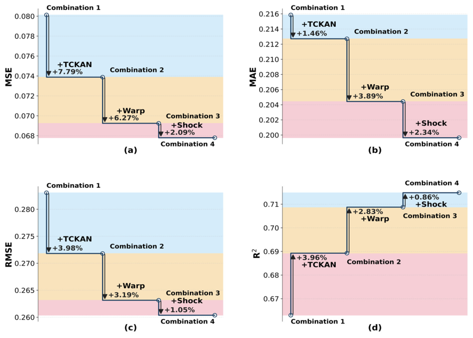
Combination	TCKAN	Warp Fourier	Shock Kernel	MSE	MAE	RMSE	R2
1	🗶	🗶	🗶	0.0801	0.2158	0.2830	0.6630
2	✔	🗶	🗶	0.0738	0.2127	0.2718	0.6892
3	✔	✔	🗶	0.0692	0.2044	0.2631	0.7087
4	✔	✔	✔	0.0677	0.1996	0.2603	0.7148

Note: cross (🗶) indicates that the module was not included in that combination, while a check (✔) indicates that the module was included.

. Combination 1 is the Prophet baseline without TCKAN or WFSK. Combinations 2 to 4 successively add the TCKAN module, the Warped Fourier module, and the Shock Kernel module. This isolates the marginal contribution of each component. As shown in Table 6, MSE, MAE, and RMSE decrease consistently from Combination 1 to Combination 4. R-squared moves closer to one. This pattern confirms that each added component improves predictive accuracy.

Figure 6 synthesizes the staged gains in predictive fidelity as modules are layered. In Figure 6a, adding TCKAN yields the dominant MSE drop 7.79%, evidencing suppression of episodic high-amplitude errors; Warped Fourier adds a moderate decrement, and the Shock Kernel removes residual heavy tailed variance, forming a three-step cascade. In Figure 6b, an analogous hierarchy appears for MAE: TCKAN initiates structural tightening, frequency warping corrects drifting periodic misalignment, and the Shock Kernel excises shock dominated outliers, smoothing pointwise deviations. In Figure 6c, TCKAN’s scale-normalized robustness drop of 3.98% establishes a lower variance baseline, Warped Fourier’s drop of 3.19% exploits stabilized local encodings, and Shock Kernel’s drop of 1.05% attenuates residual volatility spikes. In Figure 6d, R² elevates in three plateaus: TCKAN supplies high-resolution local temporal structure; Warped Fourier reflects activation of drift aware spectral decomposition once locality is secured; and Shock Kernel converts transient variance into deterministic signal.

The ablation results quantify the complementary effectiveness of the Warped Fourier and Shock Kernel modules. The transition from Combination 3 (with Warped Fourier, without Shock Kernel) to Combination 4 (full model, both modules) isolates the marginal contribution of the Shock Kernel, yielding consistent improvements across all four evaluations metrics: MSE from 0.0692 to 0.0677, MAE from 0.2044 to 0.1996, RMSE from 0.2631 to 0.2603, and R-squared from 0.7087 to 0.7148. These gains are achieved on top of an already optimized base and are attributable solely to the explicit parameterization of aperiodic discontinuities. The Warped Fourier component captures continuous seasonal phase drift, while the Shock Kernel addresses abrupt transitions that smooth warping cannot represent, confirming that the two modules are complementary rather than redundant.

All modules contribute positively; the combined TCKAN–WFSK configuration remains optimal across experimental settings, confirming the complementary strengths of local feature extraction and global shock modeling.

The ablation pattern is consistent with the functional decoupling rationale of the proposed framework. Prophet separates global trend, recurring seasonality, and event terms, so the deep learner is not required to reconstruct the whole series. TCKAN then focuses on conditional residual learning from residual history, lagging exogenous inputs, and shock intensity [43]. Warped Fourier and Shock Kernel address different residual structures. The former represents smooth seasonal phase drift through monotone time warping, whereas the latter represents aperiodic event propagation through finite shock history windows and decay kernels. A smooth phase basis is not designed to model abrupt impulse decay efficiently, and a Shock Kernel is not designed to represent recurring seasonal phase shifts. Therefore, the stepwise improvement observed in the ablation study is not only associated with increased model capacity. It is consistent with a task separation among structural decomposition, nonlinear residual learning, seasonal phase adjustment, and discrete shock response [33].

4.3.4. B-Spline Weight Transparency

To elucidate the diagnostic transparency of the B-spline weight distributions in the model, we systematically examine the weight distribution of B-spline basis functions across all KAN layers and plot histograms of the absolute weight values. The external variable EUA, identified as having the highest correlation (as in Table 1), was chosen to illustrate the KAN’s response.

Four subplots are shown in Figure 7, representing the two KAN modules of TCKAN, each comprising two KAN layers. The horizontal axis represents the absolute values of the B-spline basis function weights in the KAN, reflecting the strength of each basis function, while the vertical axis indicates the count of basic functions. The weights cluster near zero, with only a few significant values, indicating selective feature processing. Compared to the first KAN layer, the second KAN layer shows a broader weight distribution, reflecting enhanced capacity for modeling complex interactions. This hierarchical sparsity enables automatic focus on critical input regions while suppressing irrelevant components. Variations across layers and models reveal adaptive nonlinear responsiveness. This data-driven structural adaptation provides diagnostic transparency by showing how spline parameters are selectively activated. This establishes a structural basis for robust generalization, particularly in out-of-distribution scenarios.

To quantify transparency beyond qualitative visualization, we computed sparsity ratios from the B-spline weight matrices of the trained KAN model. The TCKAN backbone comprises four KAN layers containing a total of 21,248 spline parameters. In this evaluation, a defined threshold specifies the cutoff magnitude for the absolute weight values. Parameters with absolute weights falling below this threshold are categorized as near-zero weights and are treated as inactive. Conversely, active parameters are those with absolute weights equal to or exceeding the threshold, which inherently carry effective nonlinear transformations. The sparsity ratio is thus calculated as the overall proportion of these inactive parameters.

Table 7. KAN sparsity ratios.

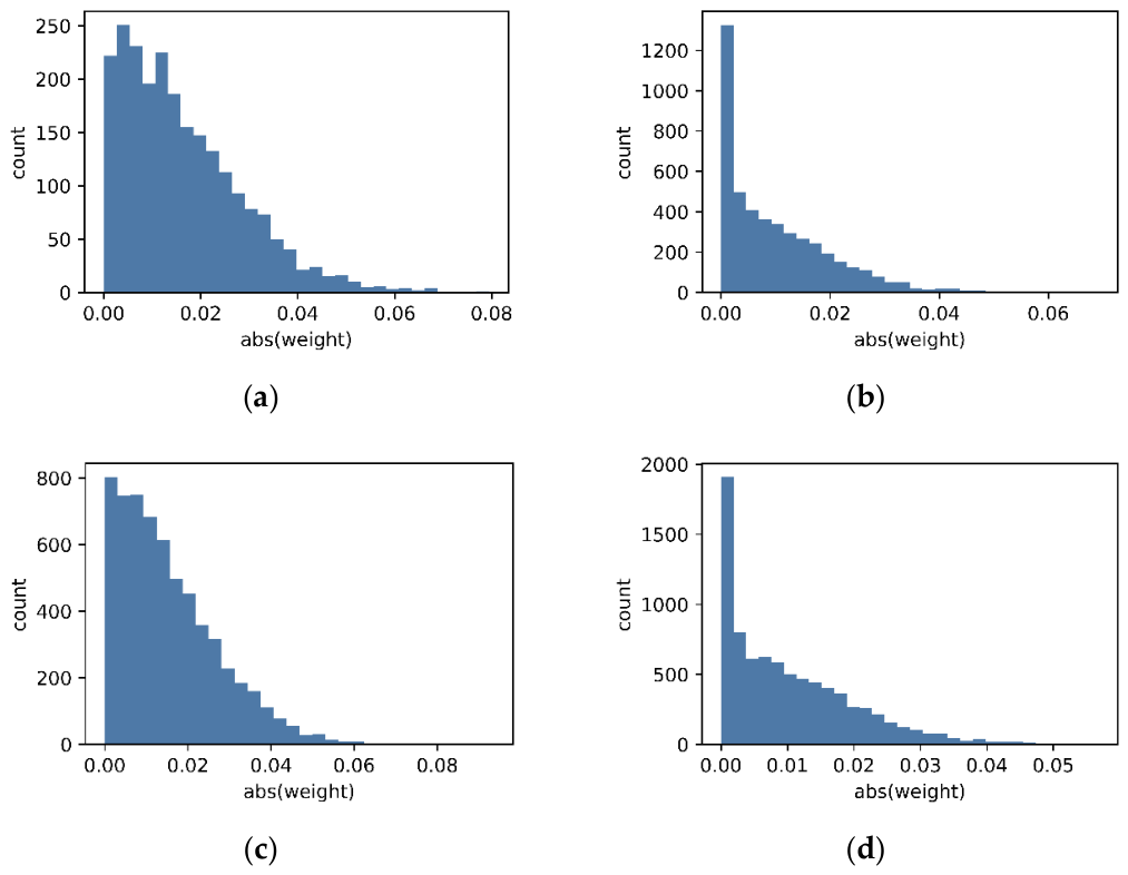
Threshold	Near-Zero Weights	Sparsity Ratio	Active Parameters
0.01	8525/21,248	40.1%	12,723 (59.9%)
0.05	20,550/21,248	96.7%	698 (3.3%)

details the fraction of near-zero weights evaluated at two specific thresholds. At a strict threshold of 0.01, approximately 40 percent of the spline weights are rendered effectively inactive. Furthermore, at a relaxed threshold of 0.05, merely 3.3 percent of the parameters retain substantial nonlinear transformations. This pronounced sparsity suggests implicit parameter level selection in the KAN layers. For a given input, only a sparse subset of B-spline basis functions is activated.

Table 8. Layer-wise sparsity at threshold 0.01.

Layer	Parameters	Near-Zero	Sparsity	Active
Block0_KAN0	2304	680	29.5%	70.5%
Block0_KAN1	4608	2240	48.6%	51.4%
Block1_KAN0	6144	1861	30.3%	69.7%
Block1_KAN1	8192	3744	45.7%	54.3%
ALL	21,248	8525	40.1%	59.9%

shows that shallow layers (Block0_KAN0 and Block1_KAN0) retain lower sparsity (29.5% and 30.3%) because they process broader input features. Deeper layers (Block0_KAN1 and Block1_KAN1) converge to higher sparsity (48.6% and 45.7%) by focusing on a smaller set of critical features. This monotonic pattern is consistent with the hierarchical abstraction expected in deep architecture.

The sparsity analysis should be interpreted as a measure of diagnostic transparency rather than full economic interpretability. It quantifies how many B-spline basis functions are effectively inactive and how many remain active in the trained KAN layers. This diagnostic is not directly available in standard deep learning baselines, because these models do not expose edge-wise spline activation functions or layer-wise basis activation weights. Therefore, the comparison with existing deep learning forecasting models is structural rather than numerically symmetric. The proposed TCKAN provides an internal sparsity-based diagnostic of nonlinear activation, while conventional deep learning baselines usually require additional post hoc explanation tools to inspect their internal representations. This distinction supports the claim of improved diagnostic transparency, but it does not imply full interpretability or direct mapping to economic mechanisms.

4.3.5. Robustness Analysis

The robustness of the model is assessed by varying the training–test split and the time window size. All other experimental settings are held constant. EUA is selected as the representative uncertainty feature. The baseline hyperparameters are kept at the values used in the main comparative experiments. Only the relevant parameters are varied in each test.

As reported in

Table 9. Robustness test with uncertainty risk.

Parameters	Model	MAE	RMSE	DM
Ratio = 6:1:3	Prophet-TCKAN-WFSK	0.1918 ± 0.0156	0.2562 ± 0.0166
	TimesNet	0.2407 ± 0.0214	0.3356 ± 0.0218	−2.5460 **
	Autoformer	0.2363 ± 0.0198	0.3201 ± 0.0207	−2.5119 **
	TimeMixer	0.2193 ± 0.0200	0.3090 ± 0.0200	−1.6448 *
	SARIMA	0.3637 ± 0.0335	0.5153 ± 0.0334	−6.2138 ***
	ARIMA-GARCH	0.3446 ± 0.0325	0.4945 ± 0.0321	−5.6108 ***
	TBATS	0.5302 ± 0.0587	0.8310 ± 0.0539	−7.0957 ***
Ratio = 8:1:1	Prophet-TCKAN-WFSK	0.2746 ± 0.0234	0.3747 ± 0.0243
	TimesNet	0.3017 ± 0.0199	0.3719 ± 0.0241	−1.1968
	Autoformer	0.2831 ± 0.0210	0.3642 ± 0.0236	−0.4612
	TimeMixer	0.2843 ± 0.0205	0.3618 ± 0.0235	−0.5577
	SARIMA	0.3947 ± 0.0286	0.5034 ± 0.0326	−3.0323 ***
	ARIMA-GARCH	0.3865 ± 0.0287	0.4973 ± 0.0322	−2.6562 **
	TBATS	0.3594 ± 0.0357	0.5298 ± 0.0343	−3.1420 ***
Ratio = 7:2:1	Prophet-TCKAN-WFSK	0.2484 ± 0.0191	0.3241 ± 0.0210
	TimesNet	0.3957 ± 0.0264	0.4891 ± 0.0317	−4.4818 ***
	Autoformer	0.2592 ± 0.0196	0.3362 ± 0.0218	−0.5829
	TimeMixer	0.2843 ± 0.0205	0.3618 ± 0.0235	−1.4271 *
	SARIMA	0.3899 ± 0.0289	0.5011 ± 0.0325	−4.1622 ***
	ARIMA-GARCH	0.3777 ± 0.0293	0.4945 ± 0.0321	−3.6531 ***
	TBATS	0.3972 ± 0.0352	0.5526 ± 0.0358	−4.6283 ***
Window size = 3	Prophet-TCKAN-WFSK	0.1881 ± 0.0155	0.2530 ± 0.0164
	TimesNet	0.2253 ± 0.0294	0.3920 ± 0.0254	−1.1367
	Autoformer	0.3266 ± 0.0363	0.5137 ± 0.0333	−3.7100 ***
	TimeMixer	0.2372 ± 0.0316	0.4186 ± 0.0271	−1.4739 *
	SARIMA	0.2537 ± 0.0253	0.3745 ± 0.0243	−2.9550 **
	ARIMA-GARCH	0.2666 ± 0.0246	0.3781 ± 0.0245	−3.4273 ***
	TBATS	0.3572 ± 0.0327	0.5046 ± 0.0327	−7.1078 ***
Window size = 7	Prophet-TCKAN-WFSK	0.2046 ± 0.0154	0.2647 ± 0.0172
	TimesNet	0.2533 ± 0.0227	0.3540 ± 0.0229	−2.3059 **
	Autoformer	0.2167 ± 0.0198	0.3058 ± 0.0198	−0.7801
	TimeMixer	0.2104 ± 0.0186	0.2925 ± 0.0190	−0.4802
	SARIMA	0.2537 ± 0.0253	0.3745 ± 0.0243	−2.3198 **
	ARIMA-GARCH	0.2655 ± 0.0236	0.3696 ± 0.0240	−2.8967 **
	TBATS	0.3568 ± 0.0313	0.4936 ± 0.0320	−6.5778 ***

Note: Holm–Bonferroni corrected DM test significance levels are denoted by *** $p<0.01$, ** $p<0.05$, and * $p<0.10$.

, the proposed model remains competitive across different data split ratios and window settings. It achieves strong MAE performance and maintains stable forecast accuracy under changes in data partition and input window size. Although it does not obtain the lowest RMSE in every individual setting, the results indicate that the framework is not overly sensitive to the training test split or temporal window length.

The robustness checks further cover practical data-quality and market-stress scenarios. The no-exogenous-feature experiment represents external-input loss by removing all uncertainty-risk variables and event-related covariates, forcing the model to rely on the endogenous CCFI structure. To further assess robustness,

Table 10. Lag sensitivity analysis.

Lag Configuration	MAE	RMSE
Lag = 1 (Minimal)	0.1913 ± 0.0138	0.2434 ± 0.0158
Lag = 4 (Intermediate)	0.1889 ± 0.0135	0.2395 ± 0.0155
Lag = 8 (Extended)	0.1845 ± 0.0143	0.2419 ± 0.0157

,

Table 11. Noise robustness analysis.

Noise Level	MAE	RMSE
10%	0.2035 ± 0.0163	0.2700 ± 0.0175
15%	0.2062 ± 0.0160	0.2702 ± 0.0175
20%	0.2066 ± 0.0159	0.2696 ± 0.0175

,

Table 12. Sensitivity of Warped Fourier to B-spline basis size and warp regularization coefficient.

Basis Size\Regularization	1 × 10−4	1 × 10−3	1 × 10−2
4	0.2351 ± 0.0563	0.2230 ± 0.0543	0.2378 ± 0.0570
6	0.2186 ± 0.0523	0.2153 ± 0.0517	0.2201 ± 0.0528
8	0.2160 ± 0.0518	0.2147 ± 0.0515	0.2182 ± 0.0523
10	0.2198 ± 0.0527	0.2158 ± 0.0519	0.2285 ± 0.0546

and

Table 13. Sensitivity of different kernels.

Kernel	MAE	RMSE
Composite Shock Kernel (Proposed)	0.2147 ± 0.0515	0.2818 ± 0.0680
Matérn Kernel (ν = 3/2)	0.2192 ± 0.0527	0.2875 ± 0.0694
Rational Quadratic Kernel	0.2240 ± 0.0537	0.2938 ± 0.0709
Laplacian Kernel	0.2273 ± 0.0545	0.2980 ± 0.0719

report a set of complementary checks. Table 10 examines lag sensitivity, Table 11 tests robustness to noisy observations, Table 12 evaluates the sensitivity of the Warped Fourier module to basis size and warp regularization, and Table 13 compares alternative Shock Kernel functions. Together, these tests examine whether the framework is sensitive to lag choices, input noise, seasonal-warp settings, or kernel specification. Robustness under extreme market stress is further examined through the cross-regime experiment, where the model is trained on pre-May 2020 observations and tested during the May 2020–June 2021 pandemic regime without retraining. These settings provide evidence of robustness to unavailable external information, noisy observations, and unseen regime stress. They focus on external-input loss rather than exhausting all possible missing-data mechanisms, such as random deletion or block missingness.

Lag Sensitivity: As shown in Table 10, a key practical concern is whether forecast accuracy depends critically on precise lag specification. Table 10 reports performance across three lag configurations: Lag = 1 (minimal), Lag = 4 (intermediate), and Lag = 8 (extended). MAE varies by only 3.6% across configurations, ranging from 0.1845 to 0.1913. All three specifications achieve comparable performance, with the extended lag (Lag = 8) yielding a modest 3.6% improvement over the minimal specification. This robustness stems from the TCKAN gating mechanism’s ability to adaptively weight temporal features, compensating for suboptimal lag specifications through learned feature selection.

Noise Robustness: Real-time economic indicators often contain measurement errors and delays. To simulate these conditions, Gaussian noise was injected into the exogenous variable at levels of 10%, 15%, and 20% of the feature’s standard deviation. Table 11 reports forecast accuracy under noise perturbations. The framework exhibits strong robustness, which stems from three architectural defenses: Prophet’s robust decomposition, the TCKAN gating mechanism, and the WFSK curvature penalty.

Warped Fourier Sensitivity: To examine whether the Warped Fourier module is sensitive to its internal parameter setting, we conduct a grid sensitivity analysis over the B-spline basis size and the warp regularization coefficient. The tested basis sizes are 4, 6, 8, and 10. The tested regularization coefficients are 1 × 10⁻⁴, 1 × 10⁻³ and 1 × 10⁻². Table 12 reports MAE on normalized data under these settings. The results show that the best performance is obtained with basis size 8 and regularization coefficient ${10}^{-3}$, where MAE reaches 0.2147. Basis size 4 yields higher errors, indicating that too few basis functions may underfit seasonal phase drift. A larger basis size does not necessarily improve performance, as basis size 10 shows higher MAE under stronger regularization. Overall, the results indicate that the Warped Fourier module performs stably within a moderate parameter range and that the selected setting balances phase flexibility and smoothness control.

Shock Kernel Comparison: An additional comparison of kernel types confirms the empirical advantage of the proposed Composite Shock Kernel. Table 13 reports MAE and RMSE for four kernel configurations. The Composite Shock Kernel achieves the lowest errors, whereas Matérn, Rational Quadratic, and Laplacian kernels result in higher MAE and RMSE values. This confirms that the proposed kernel effectively models discrete event shocks and their decay, contributing complementary predictive value within the overall TCKAN–WFSK framework. These results also indicate that the module is robust across reasonable hyperparameter settings and that performance gains arise from the functional design rather than arbitrary parameter selection.

4.3.6. Generalization Ability

As shown in

Table 14. Generalizability test with uncertainty risks.

Feature	Model	MAE	RMSE	DM
WTI	Prophet-TCKAN-WFSK	0.1553 ± 0.0088	0.1825 ± 0.0118
	TimesNet	0.1733 ± 0.0176	0.2584 ± 0.0167	−0.7375
	Autoformer	0.2531 ± 0.0225	0.3528 ± 0.0229	−2.9448 **
	TimeMixer	0.1808 ± 0.0184	0.2701 ± 0.0175	−0.9954
	SARIMA	0.4771 ± 0.0406	0.6511 ± 0.0422	−5.6880 ***
	ARIMA-GARCH	0.5001 ± 0.0397	0.6619 ± 0.0429	−6.2342 ***
	TBATS	0.4650 ± 0.0491	0.7089 ± 0.0460	−4.2675 ***
LNG_160	Prophet-TCKAN-WFSK	0.1830 ± 0.0105	0.2161 ± 0.0140
	TimesNet	0.1981 ± 0.0173	0.2739 ± 0.0178	−0.5925
	Autoformer	0.2362 ± 0.0201	0.3223 ± 0.0209	−1.8920 *
	TimeMixer	0.1988 ± 0.0171	0.2727 ± 0.0177	−0.6148
	SARIMA	0.4771 ± 0.0442	0.6782 ± 0.0440	−4.9968 ***
	ARIMA-GARCH	0.4906 ± 0.0430	0.6785 ± 0.0440	−5.3342 ***
	TBATS	0.4650 ± 0.0491	0.7089 ± 0.0460	−4.0024 ***
TP_EMA	Prophet-TCKAN-WFSK	0.1957 ± 0.0117	0.2334 ± 0.0151
	TimesNet	0.2115 ± 0.0208	0.3098 ± 0.0201	−0.5215
	Autoformer	0.2755 ± 0.0236	0.3770 ± 0.0244	−2.2948 **
	TimeMixer	0.2049 ± 0.0213	0.3098 ± 0.0201	−0.2819
	SARIMA	0.4720 ± 0.0407	0.6479 ± 0.0420	−5.0406 ***
	ARIMA-GARCH	0.4806 ± 0.0404	0.6519 ± 0.0423	−5.1957 ***
	TBATS	0.4650 ± 0.0491	0.7089 ± 0.0460	−3.8736 ***
EUA	Prophet-TCKAN-WFSK	0.1521 ± 0.0089	0.1803 ± 0.0117
	TimesNet	0.1906 ± 0.0180	0.2740 ± 0.0178	−1.6389 *
	Autoformer	0.2088 ± 0.0157	0.2700 ± 0.0175	−2.3979 **
	TimeMixer	0.1801 ± 0.0160	0.2510 ± 0.0163	−1.2879
	SARIMA	0.4755 ± 0.0406	0.6499 ± 0.0421	−5.8662 ***
	ARIMA-GARCH	0.4883 ± 0.0400	0.6548 ± 0.0424	−6.1855 ***
	TBATS	0.4650 ± 0.0491	0.7089 ± 0.0460	−4.4901 ***

Note: Friedman nonparametric test indicates significant overall performance differences among the compared models in the generalization experiment $\left({\chi }^2=30.90,p<0.001\right)$. The proposed Prophet-TCKAN-WFSK model achieves the best average rank (1.25 out of 7), indicating the strongest overall rank-based performance under the cross-regime generalization setting. The Nemenyi post hoc test further shows significant rank advantages over TimeMixer, ARIMA GARCH, and TBATS. The differences against TimesNet, Autoformer, and SARIMA remain positive but do not exceed the conservative critical difference. Holm–Bonferroni corrected DM test significance levels are denoted by *** $p<0.01$, ** $p<0.05$, and * $p<0.10$.

, to evaluate out-of-distribution generalization under regime shifts, a temporal split experiment is conducted in which the model is trained on pre-May 2020 data and tested on the May 2020–June 2021 pandemic period. This configuration creates a sharp distributional shift: the test period contains unprecedented volatility and structural breaks (BP1 and BP2, Section 4.1) that are absent from the training data. Despite this regime discontinuity, the proposed framework maintains stable predictive performance under this cross-regime setting.

The out-of-distribution testing also provides evidence of breakpoint robustness. The model is trained exclusively on pre-COVID-19 data (before May 2020) and tested on mid-COVID-19 data (May 2020 to June 2021), creating a sharp distributional shift at the breakpoint. This test period is not treated as a clean single-shock setting. It contains overlapping uncertainty channels, including pandemic restrictions, port and supply-chain congestion, continuing trade-policy pressure, and energy-market volatility. Despite this regime discontinuity, the proposed framework maintains stable and consistent predictive performance across all exogenous variable configurations under this sharp distributional shift. The event-window encoder allows concurrent event increments to enter the same historical window. The Shock Kernel then models their joint propagation and decay. The gating mechanism reweighs the residual, seasonal, and shock components according to the current temporal state. This cross-regime generalization indicates that the results are not solely driven by an arbitrary segmentation choice. The selection of May 2020 as the primary breakpoint is further justified by Bai–Perron structural break tests reported in Section 4.1, which identify this date as the most significant regime shift in the sample period. Therefore, the same experiment also provides a stress test for overlapping uncertainty effects. It evaluates whether the model can remain stable when several uncertainty channels affect the freight market at the same time. It does not aim to identify the separate causal contribution of each concurrent stick. Together, these results demonstrate that the framework maintains stable predictive performance under a statistically justified structural break.

The baseline comparisons in Table 14 should be interpreted as supplementary performance references. The main purpose of this experiment is to evaluate cross-regime generalization. The model is trained on data before the COVID-19 period and tested during the COVID-19 period without retraining. This setting examines whether the framework can maintain predictive performance under an unseen structural shift.

4.4. Empirical Analysis

Across three stages, namely pre-COVID-19, mid-COVID-19, and post-COVID-19, this study employs a dynamic event window strategy with an expanding training scheme. This three-stage design evaluates adaptation after structural breaks. It does not claim to predict structural breaks before they occur. A fixed test set is maintained across all three stages. The fixed test set is defined as the final chronological holdout period. Its length is determined according to the overall size of the weekly dataset. This choice preserves sufficient observations for model training. It also retains an adequate out-of-sample period for evaluation. The training data are progressively expanded. Stage 1 uses only data before COVID-19. Stage 2 adds observations during COVID-19. Stage 3 uses all available training data before the fixed test period. The fixed test set is strictly excluded from all training stages. Correspondingly, the Prophet event terms are constructed only from the major events available within each training stage, as defined in Table 2. Events in the fixed test set are not used during training. Since the test period remains unchanged, performance changes across stages reflect how the model uses additional regime information when such information becomes available. This design complements the out-of-distribution test in Section 4.3.6. Section 4.3.6 evaluates cross-regime prediction without retraining. Section 4.4 evaluates adaptation under progressively expanded training information. Together, the two analyses distinguish prediction across an unseen regime shift from adaptation after structural information becomes available.

Using the breakpoint proportions identified in Figure 4, the framework iteratively superimposes event impacts through dynamic time windows. This design accounts for lag effects and overlapping event effects. It helps examine risk transmission mechanisms under external shocks. All input data are normalized to reduce scale differences. Logarithmic scaling is used only for visualization clarity. Model performance is evaluated using Mean Absolute Error and Root Mean Square Error.

To evaluate how the framework adapts as new regime information becomes available, the staged analysis uses a progressively expanding information set. This design traces how forecasts change as historical observations and event information are gradually enriched, rather than ranking stages under equal-sample conditions. As a result, a certain asymmetric training data issue remains across stages. This asymmetry is part of the progressive adaptation design, not an unintended split inconsistency. Accordingly, stage-to-stage changes should be interpreted as the combined effect of additional observations and newly available event information, not as a pure equal-sample performance comparison. The full chronological training procedure is summarized in Algorithm A1 in Appendix C.

4.4.1. Forecasting for Pre-COVID-19

Figure 8 presents test set results under all uncertainty risks during the pre-COVID-19 period, organized per Table 1 into Figure 8a economic and trade policy, Figure 8b spot freight index, and Figure 8c energy and carbon market (subsequent experiments follow the same layout). Two pronounced turning points in the CCFI emerge around August 2023 (Turning Point 1) and October 2024 (Turning Point 2), evidencing abrupt shifts in CCFI. In Figure 8a, the forecast trajectories are highly convergent, indicating that policy-related predictors exerted a consistent and strongly interlinked influence on CCFI before COVID-19. In Figure 8b, the C3 cluster (LNG spot rates) deviates markedly from the other series with a pronounced downward inflection at the first turning point, highlighting LNG spot dynamics as the forecasting relevance of CCFI variation in that interval. In Figure 8c, forecasts are noticeably more dispersed, implying that, in the pre-COVID-19 setting, the energy and carbon market signals distribute their influence over CCFI less uniformly; within this group, WTI and Brent exhibit the most coherent and accurate behavior, underscoring the relatively stronger explanatory power of traditional crude benchmarks for container freight movements at that stage. This first stage evaluates model performance under specific conditions.

Figure 8 reports the Stage 1 results of the progressive adaptation analysis. In this stage, the model is trained using pre-COVID-19 data only. This setting provides the baseline case before additional information becomes available. The results in Figure 8 should therefore be interpreted together with the Stage 2 and Stage 3 results. This comparison examines how forecasting behavior changes as training information expands across different structural conditions.

Table 15. Pre-COVID-19 forecast evaluation.

Index	MAE	RMSE	Index	MAE	RMSE
EUA	0.2261	0.2766	CCBFI	0.2462	0.3018
CRB	0.2338	0.2956	EPUC	0.2231	0.2732
CEA	0.2108	0.2663	LNG-160	0.2266	0.2883
WTI	0.2303	0.2983	TPU-US	0.2060	0.2549
Brent	0.2232	0.2891	C1	0.2071	0.2698
HGS	0.2364	0.2897	C2	0.2462	0.3018
LNG-145	0.2120	0.2737	C3	0.2101	0.2729
TP-EMA	0.1969	0.2443	C4	0.2240	0.2837
EPU-US	0.2194	0.2766	C5	0.2358	0.3015
GEPU	0.2073	0.2609	C6	0.2072	0.2639

examines the impact of varying uncertainty risks on model performance. In energy and carbon markets, Brent has the strongest effect on the CCFI, highlighting the influence of international oil price volatility. Among trade and economic policy risks, EPU-US performs best, emphasizing the critical role of the largest consumer market in shaping container shipping dynamics. This analysis focuses solely on pre-COVID-19 events, identifying traditional energy market factors and U.S.–China economic policy as key uncertainty risk drivers for the CCFI. These findings establish a baseline for evaluating more complex risk factors in subsequent analyses.

4.4.2. Forecasting for Mid-COVID-19

Figure 9a exhibits a more complex overall pattern, reflecting the significant global economic and trade impact of the pandemic on the CCFI. Notably, the TPU-US route stands out, highlighting the extreme effects of the combined influence of COVID-19 and China–U.S. trade tensions on the CCFI. Figure 9b also shows marked fluctuations compared to the pre-COVID-19 period. In Figure 9c, energy and carbon market uncertainty risks are more passively influenced, contributing to a more intricate forecast pattern. This is consistent with earlier findings (see Table 13), which identified traditional energy market factors and U.S.–China economic policy as the main sources of uncertainty before COVID-19, with the pandemic introducing new dynamics. The enhanced turning-point prediction capability shown in Figure 9 further demonstrates our model’s adaptability to pandemic-induced changes.

Table 16. Mid-COVID-19 forecast evaluation.

Index	MAE	RMSE	Index	MAE	RMSE
EUA	0.2080	0.2650	CCBFI	0.2194	0.2798
CRB	0.2387	0.3062	EPUC	0.2101	0.2624
CEA	0.2085	0.2660	LNG-160	0.2201	0.2827
WTI	0.2181	0.2864	TPU-US	0.2125	0.2923
Brent	0.2144	0.2825	C1	0.1964	0.2591
HGS	0.2170	0.2826	C2	0.2194	0.2798
LNG-145	0.2162	0.2835	C3	0.2129	0.2731
TP-EMA	0.1942	0.2477	C4	0.2179	0.2758
EPU-US	0.2022	0.2607	C5	0.2289	0.2944
GEPU	0.2144	0.2600	C6	0.2087	0.2714

reports the detailed experimental results as event stacking and dynamic window expansion progress, incorporating the events listed in Table 2. Compared to pre-COVID-19, trade and economic policy uncertainty risks become more dominant, accompanied by a significant reduction in forecast error metrics for most trade and economic uncertainties. Moreover, uncertainty clusters C1 (trade policy uncertainty) and C6 (economic policy uncertainty) show stronger influence in mid-COVID-19, suggesting a clustered effect. In energy markets, traditional energy’s predictive power for CCFI remains limited, whereas clean energy and carbon markets gained importance; EUA prices and LNG spot rates (C3) saw increased predictive contributions.

4.4.3. Forecasting for Post-COVID-19

The forecasting results in Figure 10 demonstrate that as the dynamic event window advances, event linkages and cumulative effects become more fully articulated, strengthening the model’s predictive capacity for the CCFI; overall forecast fidelity in Figure 10 improves markedly. In Figure 10a, the extreme impact of the pandemic gradually subsides, and the trajectory remains largely consistent, underscoring the sustained, coherent, and convergent influence of economic and trade policy factors on the CCFI. In Figure 10b, the improvement in accuracy indicates a gradual weakening of COVID-19’s disruptive effects on maritime transport. Notably, the enhanced performance of the C3 curve demonstrates the rising predictive influence of LNG on the CCFI. In Figure 10c, the forecast concentration for energy and carbon market variables begins to increase, suggesting that as the event structure matures, the energy complex progressively synchronizes and diverse negative shocks diminish. The cumulative layering and lagged transmission of shocks allow the model to capture increasingly intricate interactions and response patterns, further evidencing its stable forecasting performance under uncertainty-driven risk conditions.

As the dynamic event window goes by, the Prophet-TCKAN-WFSK model captures richer information, with every uncertainty risk specification in

Table 17. Post-COVID-19 forecast evaluation.

Index	MAE	RMSE	Index	MAE	RMSE
EUA	0.1952	0.2527	CCBFI	0.2094	0.2726
CRB	0.2306	0.2973	EPUC	0.1990	0.2557
CEA	0.2249	0.2853	LNG-160	0.2304	0.2896
WTI	0.2271	0.2937	TPU-US	0.1917	0.2484
Brent	0.2156	0.2823	C1	0.1953	0.2588
HGS	0.2159	0.2796	C2	0.2094	0.2726
LNG-145	0.2104	0.2774	C3	0.1915	0.2477
TP-EMA	0.2129	0.2636	C4	0.1903	0.2485
EPU-US	0.2016	0.2602	C5	0.2336	0.2998
GEPU	0.1794	0.2255	C6	0.1912	0.2461

achieving higher predictive accuracy than in pre-COVID-19 and mid-COVID-19. In trade and economic policy uncertainty, the deepening trade and tariff war intensifies policy shocks, disrupting global container flows and orders, while China–U.S. trade policy uncertainty escalates, with both EPU-US and EPUC reaching their highest influence on CCFI across pre-, mid- and post-COVID-19 periods; uncertainty clusters C1 (trade policy uncertainty) and C6 (economic policy uncertainty) also maintain elevated impact, evidencing sustained long-run dominance in forecast performance. From the energy market perspective, as COVID-19 restrictions unwind and border controls relax, global bulk commodity trade gradually recovers, signaling a renewed and orderly restoration of energy market influence on CCFI, with MAE and RMSE for HGS and Brent declining markedly relative to mid-COVID-19. Notably, LNG, representing cleaner energy, emerges as a key driver: since pre-COVID-19, C3 (LNG spot rate) showed growing influence, and C3 (LNG spot rate) became the strong clustering variable post-COVID-19. In parallel, the carbon market’s role strengthens substantially, and EUA exhibits the strong predictive influence among the non-clustered variables; C4 (carbon allowance) has also emerged as the most influential variable among the clustering variables.

The post-COVID-19 prediction demonstrates superior performance in reflecting CCFI fluctuations, validating the effectiveness of the dynamic event time windows approach. By adapting to major international events’ evolving nature, the proposed model captures complex interactions between CCFI and uncertainty risks more precisely, enhancing both predictive accuracy and diagnostic transparency. This aligns with earlier findings (e.g., Table 9 and Table 10), where trade and economic policy uncertainty (EPU-US, EPUC) and LNG spot rates (C3) re-emerged as dominant post-COVID-19 drivers, while energy market contributions shifted toward clean energy and carbon markets.

4.5. Discussion

This study introduces the Prophet-TCKAN-WFSK model for CCFI prediction, integrating uncertainty risks and major international events affecting container shipping (2014–2025). It effectively captures the intricate relationships between CCFI and multi-dimensional uncertainty risks (e.g., energy market volatility, trade policy shocks, and global event impacts), as demonstrated in its adaptive response to COVID-19 structural breaks (BP1/BP2 in Figure 4) and post-COVID-19 risk dynamics.

In pre-COVID-19, falling oil prices lowered shipping fuel costs, contributing to CCFI declines and overcapacity while reshaping cost structures and accelerating new energy adoption in the sector, partly driven by geopolitical shifts. Concurrently, political changes in Europe and the U.S., along with China–U.S. trade tensions, introduced global trade policy uncertainties, causing CCFI and freight rate volatility. The oil price drops further compounded these dynamics by reducing operational costs, intensifying overcapacity pressures, and incentivizing the maritime industry’s transition to cleaner energy amid geopolitical influences.

As events and policy information evolve, the COVID-19 pandemic’s impact on shipping markets becomes increasingly evident. Mid-COVID-19 data reveals that reduced reliance on traditional energy sources has heightened industry focus on energy efficiency, emissions reduction, and clean energy adoption, accelerating the sector’s green transition away from fossil fuels. This trend aligns with shifts in oil and LNG market dynamics observed in the Prophet-TCKAN-WFSK model when incorporating COVID-19-related factors. Simultaneously, trade restrictions and CCFI volatility during the crisis triggered severe disruptions in container shipping, amplifying trade policy uncertainty and exerting downward pressure on global economies—a phenomenon compounded by geopolitical tensions and pre-COVID-19 overcapacity challenges.

While the COVID-19 pandemic’s direct impact on geopolitical conflicts, trade, and economies has waned with the integration of event information, its lingering effects on the CCFI persist as a potential risk to future stability. The energy crisis, exacerbated by pandemic disruptions and extreme weather events, has amplified the influence of LNG and other clean energy sources on the CCFI, mirroring the pre-COVID-19 trend of accelerated green transition. Concurrently, carbon neutrality goals have gained broader market traction, driving industry focus toward clean energy adoption. Trade tensions, particularly between China and the U.S., continue to drive CCFI volatility and global economic uncertainty, underscoring the complex interplay among pandemic legacy, energy transition, and geopolitical dynamics in shaping shipping markets.

To strictly evaluate parameter sensitivity, we conducted robustness tests across varying data partition ratios and input window sizes, as detailed in Table 9. First, regarding data partitioning, adjusting the training–validation–test ratios simulates different data availability scenarios. Reducing the training set in the 6:1:3 ratio tests the model’s learning efficiency under limited data; the model achieves strong accuracy in this setting, suggesting that the TCKAN backbone can use limited training data effectively. Conversely, increasing the training proportion in the 8:1:1 and 7:2:1 ratios test generalization against overfitting. Despite the constrained test sets in these scenarios, the model maintains stable performance, indicating that the Shock Kernel effectively prevents the model from memorizing historical noise, ensuring robust extrapolation even when validation data is scarce. Second, regarding the window size, varying the sequence length alters the model’s temporal receptive field. Narrowing the window to 3 weeks limits historical context, resulting in a slight accuracy drop, which suggests that short-term data alone is insufficient to fully characterize complex risk transmission. Expanding the window to 7 weeks yields the best precision, confirming that extended receptive fields are critical for capturing the prolonged, lagged impacts of uncertainty risks. While not all pairwise comparisons reach statistical significance at the adjusted threshold, the proposed model achieves the lowest RMSE across all experimental configurations and ranks first or second in MAE in every comparison. The non-parametric Friedman test confirms significant overall heterogeneity among models, with the proposed model consistently positioned among the top-ranked methods. The weight of evidence therefore supports its superior predictive performance.

The ablation study demonstrates that each module can be linked to a specific operational capability. The nonlinear approximation of the temporal convolutional Kolmogorov–Arnold network enables reliable forecasts under data scarcity, a condition common in niche shipping routes where long historical records are unavailable. The adaptive sea-sonal tracking provided by the Warped Fourier mechanism reduces the need for manual recalibration as market seasonality evolves. The decay modeling of the Shock Kernel produces estimates of disruption recovery timelines, helping translate improved forecast accuracy into decision-support information and inventory management decisions following major events. Together, these modules help translate improved forecast accuracy into decision-support information for shipping operators.

In summary, policy uncertainty acts as a demand-side shock by directly altering trade flow expectations and supply chain configurations, while energy uncertainty manifested through fuel price volatility constitutes a cost-side shock. Together, these factors reshape global trade routes, with policy uncertainty emerging as the dominant driver of CCFI fluctuations under risk conditions. The carbon market, propelled by policy-driven demand, is increasingly becoming a key CCFI determinant, mirroring the growing influence of energy cost variables—a trend that underscores the industry’s green transition on the cost side. This study advances the Prophet-TCKAN-WFSK model by establishing optimal parameter ranges that balance explainability and generalization through adaptive sparsity, thereby overcoming traditional black-box limitations. Systematic empirical analysis supports the role of adaptive sparsity in improving diagnostic transparency and robustness, offering useful design principles for complex temporal forecasting. The proposed model’s performance under extreme shocks provides evidence of its reliability, while its application to CCFI reveals significant predictive power for shock events, providing actionable insights for shipping economy resilience.

However, while the framework effectively isolates the predictive hierarchy of these external shocks, the interpretation of these relationships must remain strictly within the bounds of data-driven forecasting. The finding that demand-side uncertainty variables exhibit stronger predictive importance than cost-side variables during periods of elevated market volatility is based on predictive feature importance analysis rather than formal causal inference. This study focuses on developing an accurate forecasting framework for operational decision support. The causal mechanisms underlying the observed predictive patterns represent an important direction for future research in shipping economics and finance. Nonetheless, the predictive importance findings provide actionable insights for freight market participants regarding which uncertainty dimensions warrant closer monitoring during volatile periods.

5. Conclusions

5.1. Suggestions

Previous studies on CCFI forecasting have focused on individual variable impacts. Few have examined complex multivariate features. Most modeling efforts stack existing models rather than designing architectures tailored to the specific structure of the CCFI. This study addresses that gap. The Prophet-TCKAN-WFSK model forecasts the CCFI under uncertainty risks. Shipping demand volatility is driven by event-related shocks and capacity constraints. These trigger container market oscillations. They also alter route-specific shipping levels and freight rates. The model uses dynamic event time windows to integrate and deepen event information. Uncertainty risk features enable precise identification of critical turning points. They also support robust data fitting. The model reveals how risk market characteristics influence the CCFI as events unfold. It yields actionable management recommendations for shipping market participants. The framework supports diagnostic transparency through interpretable parameters. The Shock Kernel learns decay rates from which disruption half-life can be derived, offering operators a quantitative basis for recovery timeline assessment. The Warped Fourier component tracks gradual shifts in seasonal patterns, informing capacity planning adjustments as market structure evolves. Translating these interpretable outputs into fully operational dashboards requires additional visualization development to maximize accessibility for non-technical stakeholders.

The proposed architecture may also be extended to other economic forecasting domains, such as carbon markets, energy markets, and commodity prices, without major changes to its core structure. These markets share several features with container freight markets, including non-stationarity, seasonal drift, policy shocks, and delayed responses to external events. Prophet can still provide structural decomposition. TCKAN can learn nonlinear residual dynamics. Warped Fourier can adjust drifting seasonal phases. The Shock Kernel can model event-shock propagation and decay. However, direct transfer of the fitted CCFI parameters should not be assumed. For each target market, the feature set, lag structure, event-window length, Shock Kernel half-life, Warped Fourier frequency set, and hyperparameters should be re-estimated. Therefore, the framework is transferable at the architectural level, but its empirical performance in other markets requires separate validation.

For the container shipping market, it is important to establish an appropriate data-sharing platform for uncertainty risk management by integrating key operational data. Unified early warning systems should be implemented for each CCFI route to mitigate potential uncertainty risks. Regulators must enact clear market regulations and robust risk feedback mechanisms. Enhanced market supervision can help prevent shipping companies from prioritizing short-term profits over uncertainty risks and engaging in improper practices.

For container shipping market participants, risk monitoring should be reinforced with continuous attention to market dynamics and policy signals. At the same time, sensitivity to regulatory changes must be heightened while accelerating the energy transition, reducing carbon emissions, and advancing digitalization and energy diversification to bolster market resilience and support sustainable industry development amid geopolitical and energy cost uncertainties.

For maritime practitioners, the framework is designed with operational deployment in mind. Training and inference are decoupled: model training occurs offline using historical data, while inference requires a single forward pass with modest measured latency under the tested setting. The decomposition components from Prophet can be precomputed and cached, eliminating their computational cost at inference time. The temporal convolution and KAN forward computations scale linearly with the number of input time steps, ensuring that prediction latency remains manageable as data frequency increases. These design choices support potential deployment in resource-constrained maritime forecasting environments.

5.2. Limitations

Although this study provides a meaningful methodological contribution to CCFI forecasting under uncertainty risks, several limitations should be considered when interpreting the results.

The empirical evidence is based on weekly CCFI data, and the available sample size remains limited. This restricts the range of high-frequency and high-dimensional validation that can be conducted in the present study. The robustness analysis considers noisy inputs, external-input loss, and extreme market conditions, but it does not fully examine all missing data mechanisms, such as random deletion, block missingness, route-level reporting gaps, or alternative imputation and masking strategies. Changes in the reporting methodology of external indicators are also not exhaustively tested. In addition, the benchmark models cover representative econometric and deep learning approaches, but they do not include every recent time series architecture. Some traditional baselines are univariate or have limited capacity to use exogenous variables, so perfect symmetry across all model comparisons is not possible.

The structural-regime analysis also has clear boundaries. COVID-19 is used as the main exogenous segmentation point, while Bai–Perron breakpoints are retained as post hoc statistical support rather than as training inputs. This design helps reduce look-ahead bias, but it does not constitute a fully data-driven regime-switching framework. The staged analysis further uses a progressively expanding information set. As a result, a certain asymmetric training data issue remains across stages. This asymmetry is linked to the progressive adaptation objective, but the stage-to-stage changes should not be interpreted as a pure equal-sample performance comparison. Moreover, the evidence for unprecedented-event robustness is mainly based on the COVID-19-period regime shift. It should not be regarded as a general guarantee for all future black-swan events.

The interpretation and deployment results should also be viewed with caution. The B-spline sparsity of KAN layers provides diagnostic transparency, but it does not provide full economic interpretability or formal causal identification. The relationships between uncertainty variables and CCFI are therefore predictive rather than causal. The computational comparison further shows that the proposed model has feasible cost under the tested short-window setting, but it is not the fastest baseline. Practical deployment in real-time or resource-constrained maritime forecasting systems still requires additional platform-level validation.

The external validity of the framework remains to be tested more broadly. The fitted model and parameter settings are calibrated to weekly CCFI data. Direct transfer to daily or hourly maritime data, SCFI, BDI, global container shipping indices, carbon markets, energy markets, or commodity prices should not be assumed. Such applications require re-estimating the feature set, lag structure, event-window length, Shock Kernel half-life, Warped Fourier frequencies, and hyperparameters. Reliable high-frequency, cross-index, and route-level operational data are often commercially sensitive or access-restricted. Broader validation across these settings is therefore left for future research.

5.3. Prospects

Building on the limitations outlined in Section 5.2, several directions remain to extend temporal resolution, structural analysis, operational deployment, and external-index validation for CCFI forecasting. First, future studies can extend the proposed framework to larger and higher frequency maritime datasets. In such settings, richer fusion mechanisms may become more useful. Attention-based fusion can be examined when the sample size and feature dimension are sufficient to support its additional parameter cost. Future work should also compare the proposed framework with emerging time series architectures, such as Informer, FEDformer, PatchTST, and N HiTS. These comparisons would help evaluate whether the current decomposition-based design remains robust as the methodological landscape continues to evolve. Future work should also examine explicit missing-data mechanisms, including random deletion, block missingness, and route-level reporting gaps, together with suitable imputation or masking strategies.

A second direction is to deepen the analysis of structural regime changes. The current study separates cross regime prediction from post break adaptation. The model is trained on pre-COVID-19 data and tested during the COVID-19 period in the out-of-distribution experiment. The three-stage analysis then evaluates adaptation when additional regime information becomes available. Future research can build on this design by conducting fine-grained breakpoint sensitivity analysis. Alternative segmentation dates can be compared systematically to test whether the results remain stable under different regime definitions. Dedicated structural break models, such as Bayesian change point models and regime switching frameworks, can also be incorporated to evaluate whether explicit break detection improves forecasting under extreme market transitions.

A third direction is to strengthen operational deployment and economic transparency. The proposed framework is designed for offline training and lightweight inference, but its deployment feasibility should be tested on resource-constrained maritime forecasting platforms. Such validation would clarify its practical value for real-time monitoring. In addition, B-spline weight sparsity provides diagnostic transparency, but it does not fully explain how learned representations correspond to economic mechanisms. Future research should examine whether learned activation patterns can be linked to known relationships between freight rates, oil prices, carbon prices, and trade policy shocks. This extension would improve the economic interpretability of the framework and make its output more useful for shipping market decision support.

A fourth direction is to strengthen operational deployment and economic transparency by evaluating the proposed framework on higher-frequency and cross-market maritime datasets. While the current study is calibrated specifically to the weekly CCFI, the framework’s architecture is structurally compatible with finer temporal resolutions and alternative indicators. Future research should extend this validation to include daily indices like the SCFI and BDI, as well as hourly freight rates, port congestion indicators, and route-level vessel-operation signals. Testing across these diverse dimensions will provide a stricter assessment of the model’s external validity and support real-time maritime decision-making in highly volatile markets. However, transitioning to higher-frequency or alternative indices means direct parameter transfer cannot be assumed. Key model components—including feature selection, lag structures, Shock Kernel half-lives, Warped Fourier frequencies, and TCKAN input windows—must be rigorously re-estimated to capture distinct shock decay patterns and seasonal drift mechanisms at different temporal resolutions. Currently, acquiring reliable high-frequency shipping data remains challenging, as many operational records are restricted or commercially sensitive. Overcoming these data bottlenecks in future studies will not only facilitate more granular predictive modeling but also yield richer economic interpretations of how uncertainty risks propagate through the global shipping network.

References

- Azab, A.; Morita, H. Coordinating truck appointments with container relocations and retrievals in container terminals under partial appointments information. Transp. Res. Part E Logist. Transp. Rev. 2022, 160, 102673. [Google Scholar] [CrossRef] [Scilit]
- Duan, Y.; Zhang, X.; Wang, X.; Fan, Y.; Liu, K. A Novel Forecasting System with Data Preprocessing and Machine Learning for Containerized Freight Market. Mathematics 2025, 13, 1695. [Google Scholar] [CrossRef] [Scilit]
- Tarkun, S. Financial market volatility and maritime freight indices: A connectedness approach. Res. Transp. Bus. Manag. 2025, 63, 101506. [Google Scholar] [CrossRef] [Scilit]
- Chen, S.; Meng, B.; Qiu, B.; Kuang, H. Dynamic effects of maritime risk on macroeconomic and global maritime economic activity. Transp. Policy 2025, 167, 246–263. [Google Scholar] [CrossRef] [Scilit]
- Ju, H.; Zeng, Q.; Haralambides, H. Consequences of freight rate volatility in liner shipping and the role of strategic alliances. Ocean Coast. Manag. 2024, 252, 107129. [Google Scholar] [CrossRef] [Scilit]
- Rodriguez-Diaz, E.; Alcaide, J.I.; Garcia-Llave, R. Challenges and Security Risks in the Red Sea: Impact of Houthi Attacks on Maritime Traffic. J. Mar. Sci. Eng. 2024, 12, 1900. [Google Scholar] [CrossRef] [Scilit]
- Tvedt, J.; Hovi, I.B. Container shipping: A market equilibrium perspective on freight rates formation post-COVID-19. Transp. Res. Part A Policy Pract. 2024, 179, 103917. [Google Scholar] [CrossRef] [Scilit]
- Khan, K.; Su, C.-W.; Tao, R.; Umar, M. How do geopolitical risks affect oil prices and freight rates? Ocean Coast. Manag. 2021, 215, 105955. [Google Scholar] [CrossRef] [Scilit]
- Yin, K.; Guo, H.; Yang, W. A novel real-time multi-step forecasting system with a three-stage data preprocessing strategy for containerized freight market. Expert Syst. Appl. 2024, 246, 123141. [Google Scholar] [CrossRef] [Scilit]
- Wu, R. How do climate risk and geopolitical risk impact shipping markets? Res. Int. Bus. Financ. 2026, 81, 103190. [Google Scholar] [CrossRef] [Scilit]
- Wang, W.; He, N.; Chen, M.; Jia, P. Freight rate index forecasting with Prophet model based on multi-dimensional significant events. Expert Syst. Appl. 2024, 249, 123451. [Google Scholar] [CrossRef] [Scilit]
- Ceyhun, G.Ç.; Keser, H.Y.; Tarkun, S. Dynamic spillovers of geopolitical risks and climate uncertainty on maritime freight markets: A connectedness decomposition approach. J. Transp. Geogr. 2026, 134, 104664. [Google Scholar] [CrossRef] [Scilit]
- Chen, X.; Lv, S.; Shang, W.-l.; Wu, H.; Xian, J.; Song, C. Ship energy consumption analysis and carbon emission exploitation via spatial-temporal maritime data. Appl. Energy 2024, 360, 122886. [Google Scholar] [CrossRef] [Scilit]
- Emami Javanmard, M.; Tang, Y.; Wang, Z.; Tontiwachwuthikul, P. Forecast energy demand, CO2 emissions and energy resource impacts for the transportation sector. Appl. Energy 2023, 338, 120830. [Google Scholar] [CrossRef] [Scilit]
- Zhu, M.; Du, Y.; Sha, M.; Jiang, Y.; Wu, Z.; Han, B. Multi-criteria carbon emission allowance allocation for liner shipping companies in China: An integrated approach based on composite indicators and zero-sum gains DEA. Ocean Coast. Manag. 2025, 270, 107909. [Google Scholar] [CrossRef] [Scilit]
- Song, E.; Zhang, X.; Ge, Y.; Yao, C.; Wang, B. Parallel TCN-BiGRU architecture with dynamic attention for ship energy consumption prediction under variable navigation conditions. Energy 2025, 337, 138601. [Google Scholar] [CrossRef] [Scilit]
- Shi, J.; Xu, J.; Chen, J.; Ye, J.; Zhu, M.; Qin, Q.; Zhou, S.; Liu, Y.; Xiang, Y. Clean energy ship application to promote carbon neutrality in global maritime industry: State governance or international supervision? Ocean Coast. Manag. 2024, 257, 107356. [Google Scholar] [CrossRef] [Scilit]
- Chen, Y.; Liu, B.; Wang, T. Analysing and forecasting China containerized freight index with a hybrid decomposition–ensemble method based on EMD, grey wave and ARMA. Grey Syst. Theory Appl. 2020, 11, 358–371. [Google Scholar] [CrossRef] [Scilit]
- Wu, J.; Fang, Q.; Ji, Y.; Zhang, Y. Forecasting dry bulk freight index for maritime decision-making: A hybrid signal decomposition and probabilistic modeling approach. Appl. Math. Model. 2026, 152, 116578. [Google Scholar] [CrossRef] [Scilit]
- Kim, D.; Lee, E.; Kamal, I.M.; Bae, H. Long-term forecasting of maritime economics index using time-series decomposition and two-stage attention. J. Forecast. 2025, 44, 153–172. [Google Scholar] [CrossRef] [Scilit]
- Jeon, J.-W.; Duru, O.; Munim, Z.H.; Saeed, N. System Dynamics in the Predictive Analytics of Container Freight Rates. Transp. Sci. 2021, 55, 946–967. [Google Scholar] [CrossRef] [Scilit]
- Zeng, Q.; Qu, C.; Ng, A.K.Y.; Zhao, X. A new approach for Baltic Dry Index forecasting based on empirical mode decomposition and neural networks. Marit. Econ. Logist. 2016, 18, 192–210. [Google Scholar] [CrossRef] [Scilit]
- Cao, Z.; Qian, T.; Zhang, S.; Song, H.; Tian, Y. Multi-Port Liner Ship Routing and Scheduling Optimization Using Machine Learning Forecast and Branch-And-Price Algorithm. J. Mar. Sci. Eng. 2025, 13, 2163. [Google Scholar] [CrossRef] [Scilit]
- Liu, M.; Zhao, Y.; Wang, J.; Liu, C.; Li, G. A Deep Learning Framework for Baltic Dry Index Forecasting. Procedia Comput. Sci. 2022, 199, 821–828. [Google Scholar] [CrossRef] [Scilit]
- Wu, H.; Gong, C. Modeling the Ningbo Container Freight Index Through Deep Learning: Toward Sustainable Shipping and Regional Economic Resilience. Sustainability 2025, 17, 4655. [Google Scholar] [CrossRef] [Scilit]
- Su, Z.; Li, J.; Pang, Q.; Su, M. China futures market and world container shipping economy: An exploratory analysis based on deep learning. Res. Int. Bus. Financ. 2025, 76, 102870. [Google Scholar] [CrossRef] [Scilit]
- Wang, W.; He, N.; Shao, P.; Zhou, J. An interpretable multi-model ensemble deep learning framework for forecasting ocean freight indices with external uncertainty factors. Marit. Econ. Logist. 2025, 27, 628–661. [Google Scholar] [CrossRef] [Scilit]
- Han, Z.; Zhu, X.; Su, Z. Forecasting Maritime and Financial Market Trends: Leveraging CNN-LSTM Models for Sustainable Shipping and China’s Financial Market Integration. Sustainability 2024, 16, 9853. [Google Scholar] [CrossRef] [Scilit]
- Baker, S.R.; Bloom, N.; Davis, S.J. Measuring Economic Policy Uncertainty. Q. J. Econ. 2016, 131, 1593–1636. [Google Scholar] [CrossRef] [Scilit]
- Kursa, M.B.; Rudnicki, W.R. Feature Selection with the Boruta Package. J. Stat. Softw. 2010, 36, 1–13. [Google Scholar] [CrossRef] [Scilit]
- Lin, G.; Lin, A.; Gu, D. Using support vector regression and K-nearest neighbors for short-term traffic flow prediction based on maximal information coefficient. Inf. Sci. 2022, 608, 517–531. [Google Scholar] [CrossRef] [Scilit]
- Reshef, D.N.; Reshef, Y.A.; Finucane, H.K.; Grossman, S.R.; McVean, G.; Turnbaugh, P.J.; Lander, E.S.; Mitzenmacher, M.; Sabeti, P.C. Detecting Novel Associations in Large Data Sets. Science 2011, 334, 1518–1524. [Google Scholar] [CrossRef] [Scilit] [PubMed]
- Granger, C.W.J. Investigating Causal Relations by Econometric Models and Cross-spectral Methods. Econometrica 1969, 37, 424–438. [Google Scholar] [CrossRef] [Scilit]
- Paparrizos, J.; Gravano, L. k-Shape: Efficient and Accurate Clustering of Time Series. In Proceedings of the 2015 ACM SIGMOD International Conference on Management of Data, Melbourne, Victoria, Australia; Association for Computing Machinery: New York, NY, USA, 2015; pp. 1855–1870. [Google Scholar]
- Jeon, J.; Iris, Ç.; Hong, S.; Lyons, A. Box rates unveiled: Predictive analytics for ocean freight rates with system dynamics and text mining under supply chain disruptions. Int. J. Prod. Econ. 2025, 286, 109669. [Google Scholar] [CrossRef] [Scilit]
- Xu, J.; Liu, S.; Wu, J.; Mo, Y.; Wang, K.; Ji, Q.; Wang, Y.-G.; Li, L. Multi-head attention driven aggregation-differentiation network for probabilistic groundwater depth forecasting and depth-stratified early warning: A multi-site efficient framework. Environ. Model. Softw. 2026, 199, 106934. [Google Scholar] [CrossRef] [Scilit]
- Zhou, M.; Yu, J.; Quan, W.; Meng, W. Research on predicting carbon emissions from air conditioning systems using Prophet-VMD-LSTM: A case study of a mall in northwest China. Energy Build. 2026, 358, 117197. [Google Scholar] [CrossRef] [Scilit]
- Wang, T.; Liu, X.; Liu, Y.; Li, X.; Fan, X. GCN-KAN: A model to extract autocorrelation graph features and fuse Kolmogorov-Arnold networks for stock price trend prediction. Appl. Soft Comput. 2026, 186, 114199. [Google Scholar] [CrossRef] [Scilit]
- Hossain, M.A.; Rahman, M.M.; Hasan, S.S.; Mahmud, A.; Bai, L. Analysis and forecasting of meteorological drought using PROPHET and SARIMA models deploying machine learning technique for southwestern region of Bangladesh. Environ. Sustain. Indic. 2025, 27, 100761. [Google Scholar] [CrossRef] [Scilit]
- Zhuo, X.; Ye, J.; Liu, H.; Lin, F. Analyzing dynamics of crude oil price amid sudden events and intervention measures: Insights from a Prophet-QR model. Appl. Energy 2025, 401, 126715. [Google Scholar] [CrossRef] [Scilit]
- Chang, H.; Yang, Z.; Zhang, Y. Forecasting daily freight flow in cold regions of China using the hybrid Prophet model considering the importance of festivals and epidemic prevention policy. Res. Transp. Bus. Manag. 2025, 59, 101294. [Google Scholar] [CrossRef] [Scilit]
- Amin, N.; Kim, Y.-W.; Kang, C.; Byun, Y.-C. Electricity load forecasting using hybrid prophet–TFT model incorporating weather data. Energy Rep. 2026, 15, 108846. [Google Scholar] [CrossRef] [Scilit]
- Yin, X.; Yu, Q.; Geng, X.; Yue, H. Efficient long-range ship trajectory forecasting via selective state space modeling and hybrid AIS fusion. Ocean. Eng. 2026, 349, 124075. [Google Scholar] [CrossRef] [Scilit]
- Chen, Z.; Zong, Y.; Wang, S.; Li, D. Improving estuarine discharge forecasting with a KAN-augmented LSTM model: A case study of the Yangtze River Estuary. J. Hydrol. Reg. Stud. 2025, 62, 102961. [Google Scholar] [CrossRef] [Scilit]
- Taylor, S.J.; Letham, B. Forecasting at Scale. Am. Stat. 2018, 72, 37–45. [Google Scholar] [CrossRef] [Scilit]
- Li, Y.; Liu, G.; Cao, Y.; Chen, J.; Gang, X.; Tang, J. WNPS-LSTM-Informer: A Hybrid Stacking model for medium-term photovoltaic power forecasting with ranked feature selection. Renew. Energy 2025, 244, 122687. [Google Scholar] [CrossRef] [Scilit]
- Lea, C.; Flynn, M.D.; Vidal, R.; Reiter, A.; Hager, G.D. Temporal Convolutional Networks for Action Segmentation and Detection. In Proceedings of the IEEE Conference on Computer Vision and Pattern Recognition (CVPR), Honolulu, HI, USA, 21–26 July 2017; IEEE: New York, NY, USA, 2017; pp. 1003–1012. [Google Scholar] [CrossRef] [Scilit]
- Liu, Z.; Wang, Y.; Vaidya, S.; Ruehle, F.; Halverson, J.; Soljačić, M.; Hou, T.Y.; Tegmark, M. KAN: Kolmogorov–Arnold Networks. In Proceedings of the International Conference on Learning Representations (ICLR), Singapore, 24–28 April 2025. [Google Scholar]
- Liu, J.; Yang, F.; Yan, K. Multi-Scale Data Fusion and AdaptiveLoss Kolmogorov–Arnold Network for multivariate time series forecasting. Inf. Fusion 2026, 125, 103454. [Google Scholar] [CrossRef] [Scilit]
- Bai, J.; Perron, P. Computation and Analysis of Multiple Structural Change Models. J. Appl. Econom. 2003, 18, 1–22. [Google Scholar] [CrossRef] [Scilit]
- Bergstra, J.; Bengio, Y. Random Search for Hyper Parameter Optimization. J. Mach. Learn. Res. 2012, 13, 281–305. [Google Scholar]
- Galdelli, A.; Fronzi, D.; Narang, G.; Mancini, A.; Tazioli, A. Groundwater level forecasting using data-driven models and vadose zone: A comparative analysis of ARIMA, SARIMAX, Prophet, and NeuralProphet. Appl. Comput. Geosci. 2025, 28, 100304. [Google Scholar] [CrossRef] [Scilit]
- Wu, H.; Hu, T.; Liu, Y.; Zhou, H.; Wang, J.; Long, M. TimesNet: Temporal 2D Variation Modeling for General Time Series Analysis. In Proceedings of the International Conference on Learning Representations (ICLR), Kigali, Rwanda, 1–5 May 2023. [Google Scholar]
- Wu, H.; Xu, J.; Wang, J.; Long, M. Autoformer: Decomposition Transformers with Auto Correlation for Long Term Series Forecasting. Adv. Neural Inf. Process. Syst. 2021, 34, 22419–22430. [Google Scholar]
- Wang, S.; Wu, H.; Shi, X.; Hu, T.; Luo, H.; Ma, L.; Zhang, J.Y.; Zhou, J. TimeMixer: Decomposable Multiscale Mixing for Time Series Forecasting. In Proceedings of the International Conference on Learning Representations (ICLR), Vienna, Austria, 7–11 May 2024. [Google Scholar]
- De Livera, A.M.; Hyndman, R.J.; Snyder, R.D. Forecasting Time Series With Complex Seasonal Patterns Using Exponential Smoothing. J. Am. Stat. Assoc. 2011, 106, 1513–1527. [Google Scholar] [CrossRef] [Scilit]
- Box, G.E.; Jenkins, G.M.; Reinsel, G.C.; Ljung, G.M. Time Series Analysis: Forecasting and Control; John Wiley & Sons: Hoboken, NJ, USA, 2015. [Google Scholar]