A Narrow-Phase Collision Detection Algorithm Based on Contact Theory in 2D

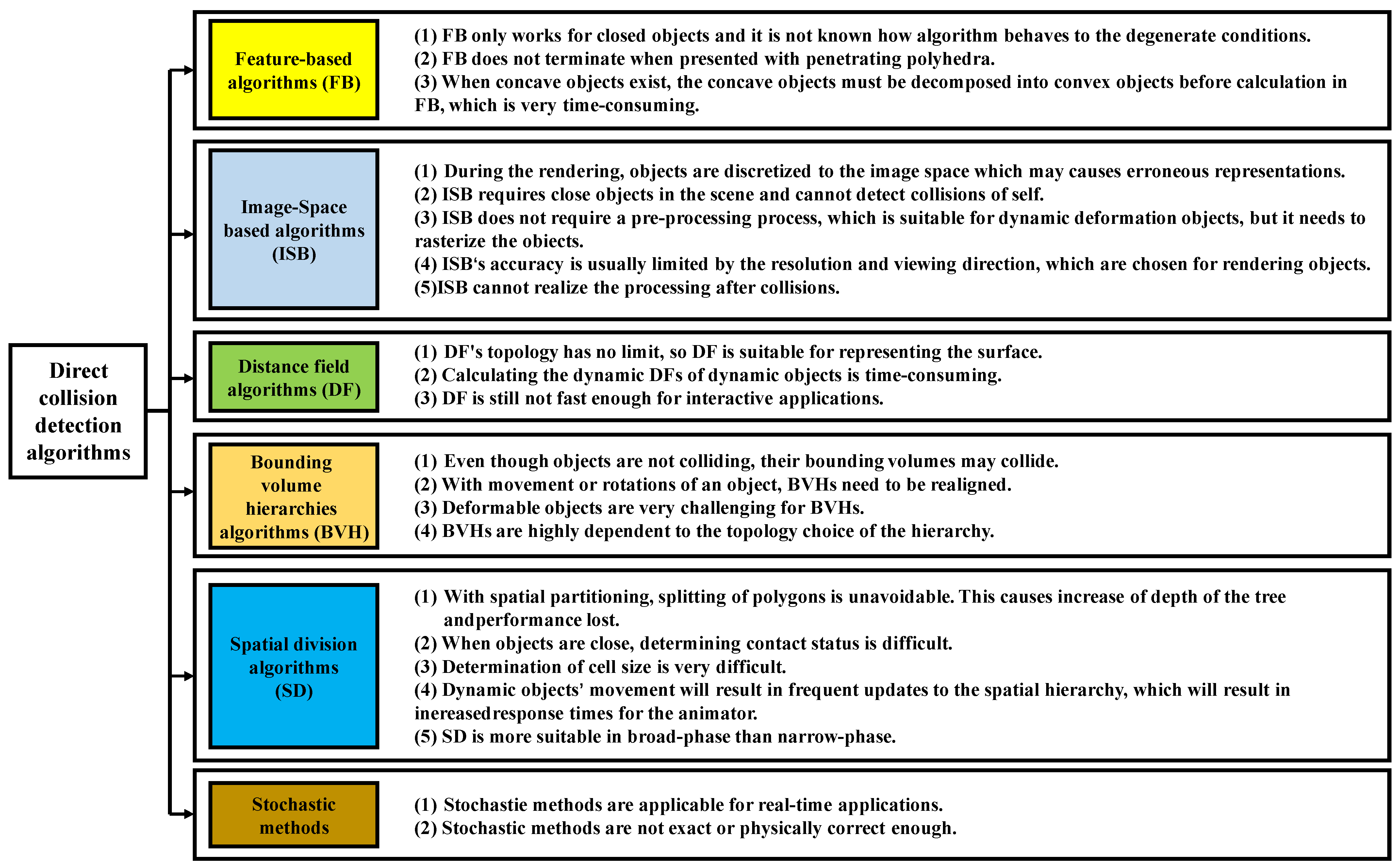
Abstract
1. Introduction
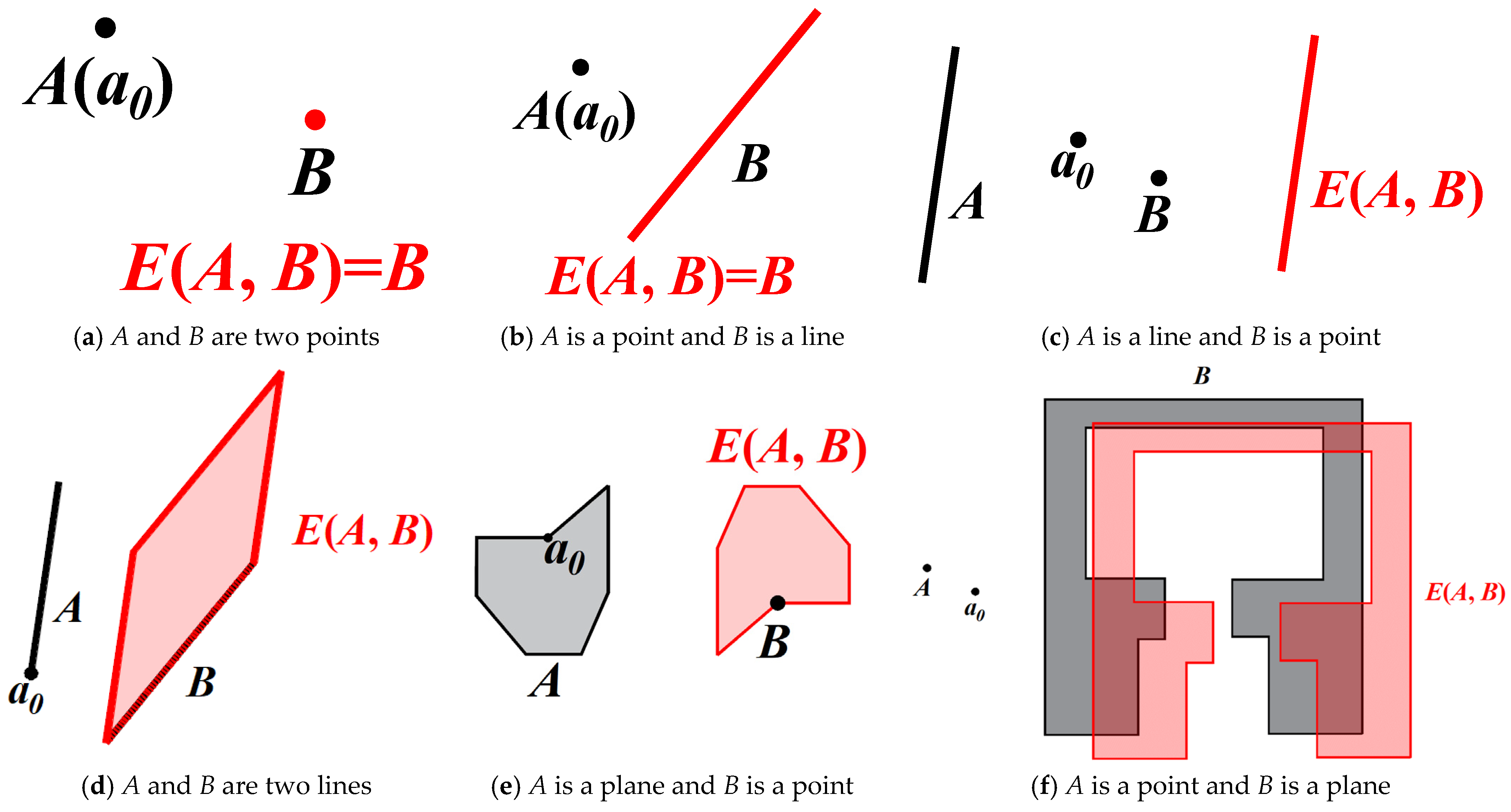
2. Introduction to Entrance Block Based on the Contact Theory
2.1. Geometrical Description of Entrance Block
2.2. Theorem of Finite Covers of Entrance Blocks
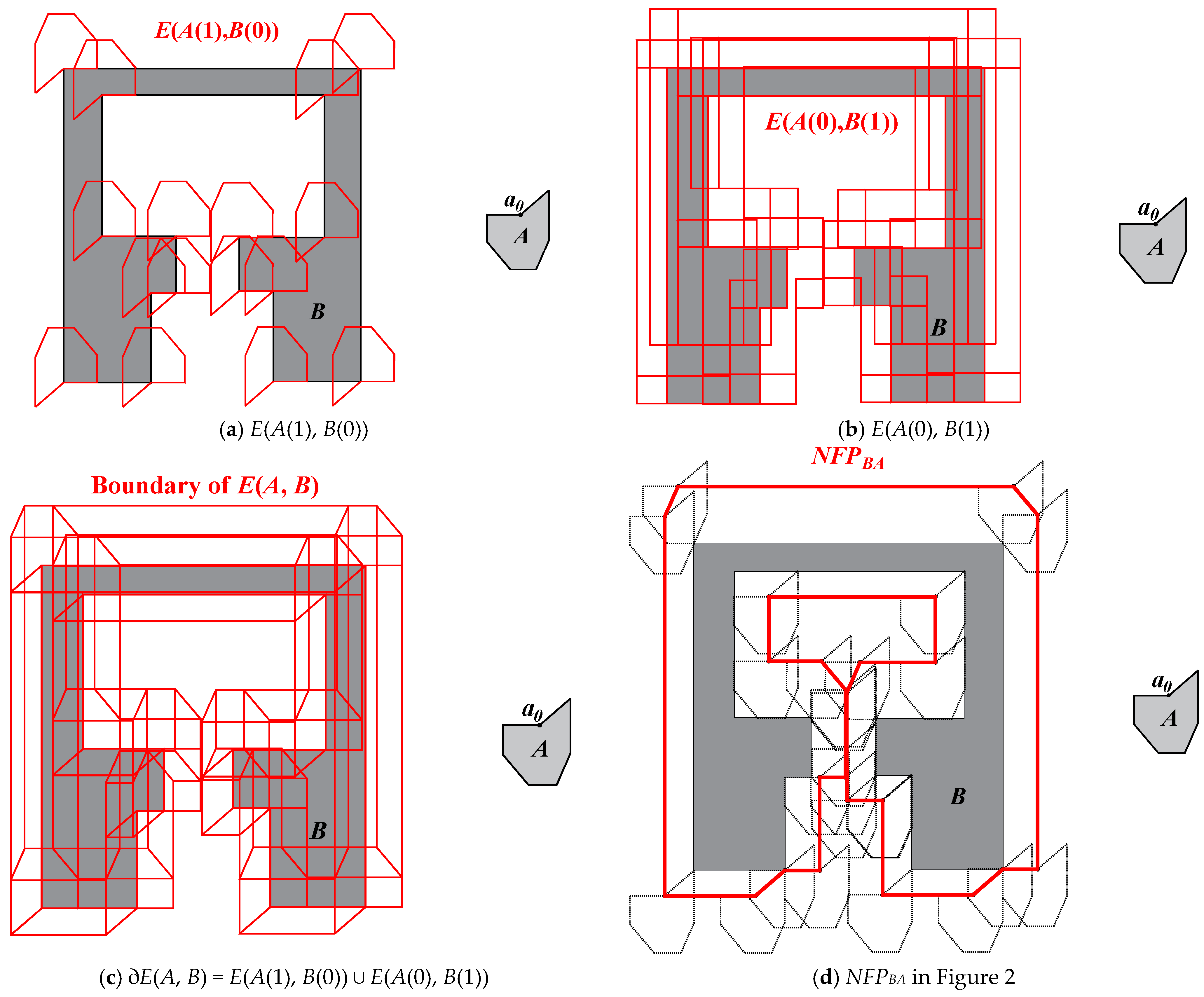
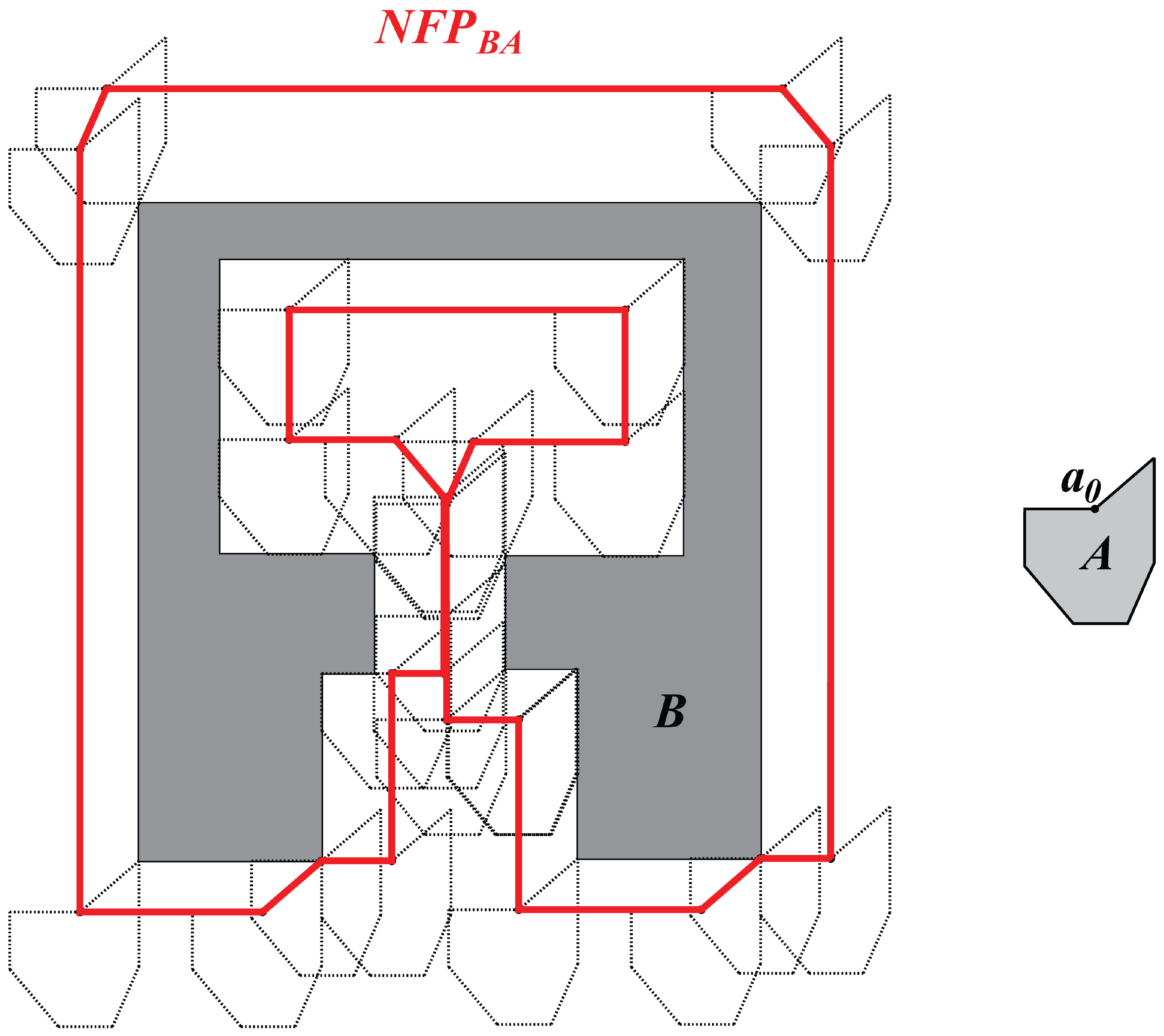
2.3. Calculation of Entrance Block Between Two 2D Objects
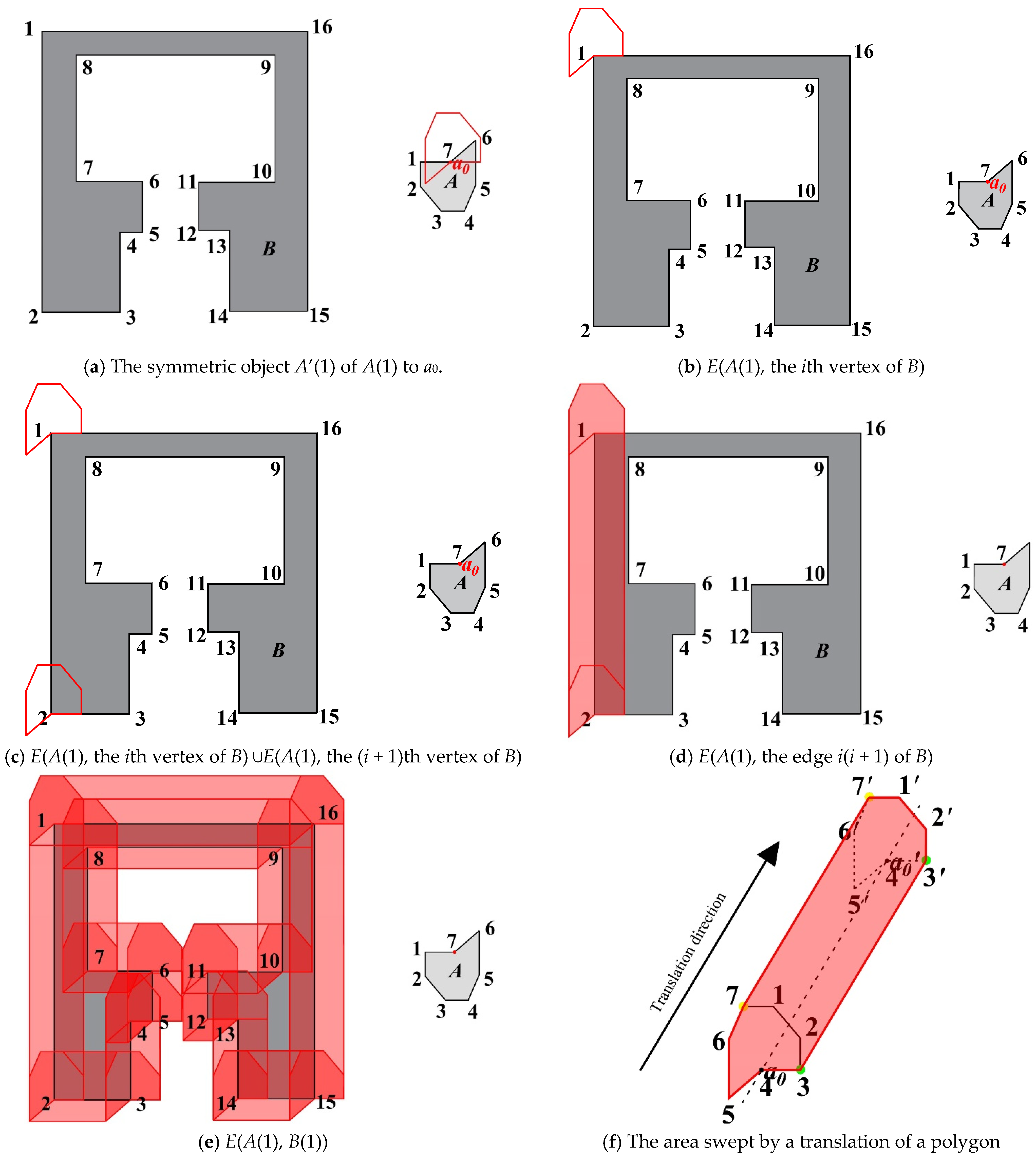
- (1)
- (2)
- (3)
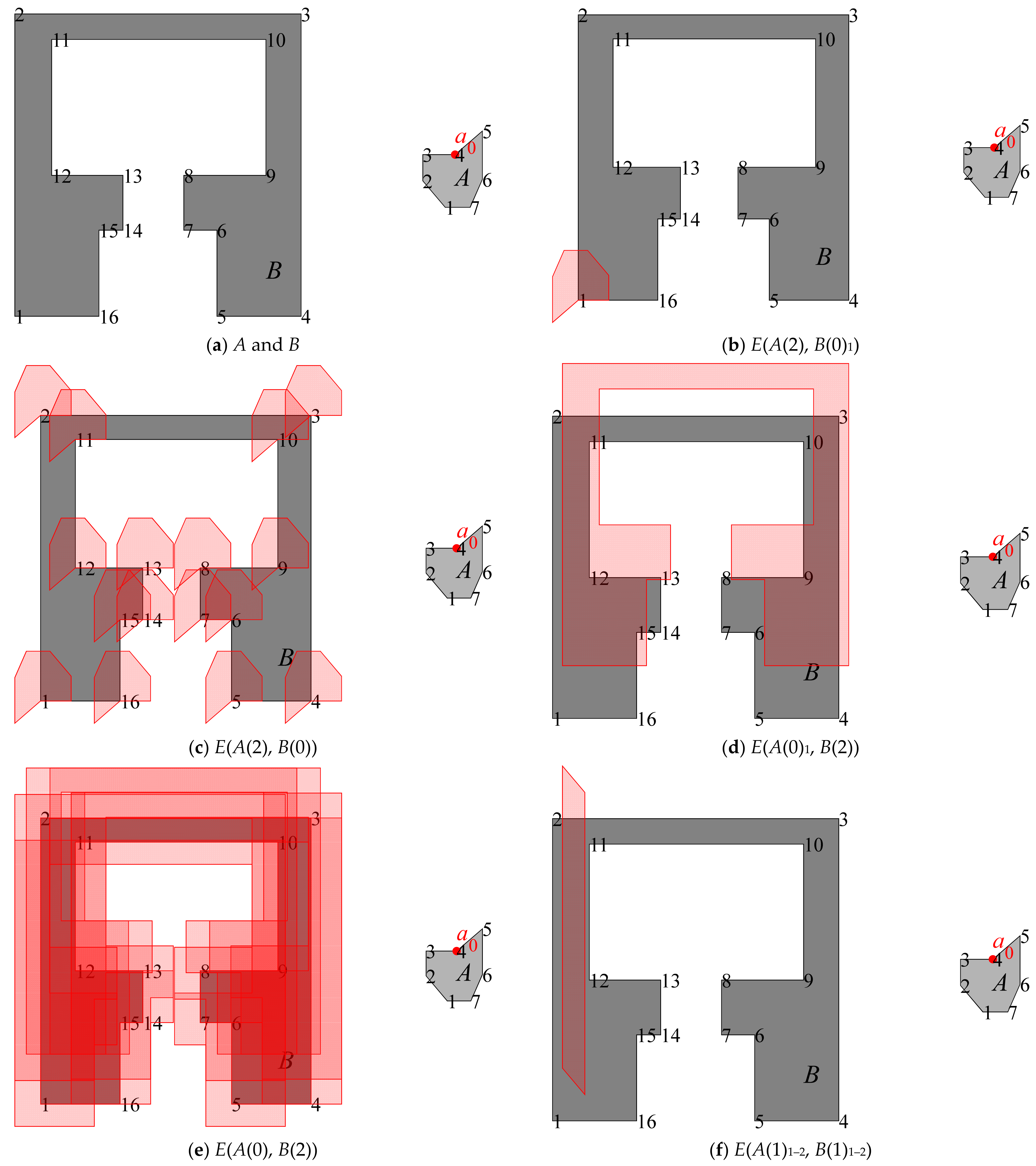
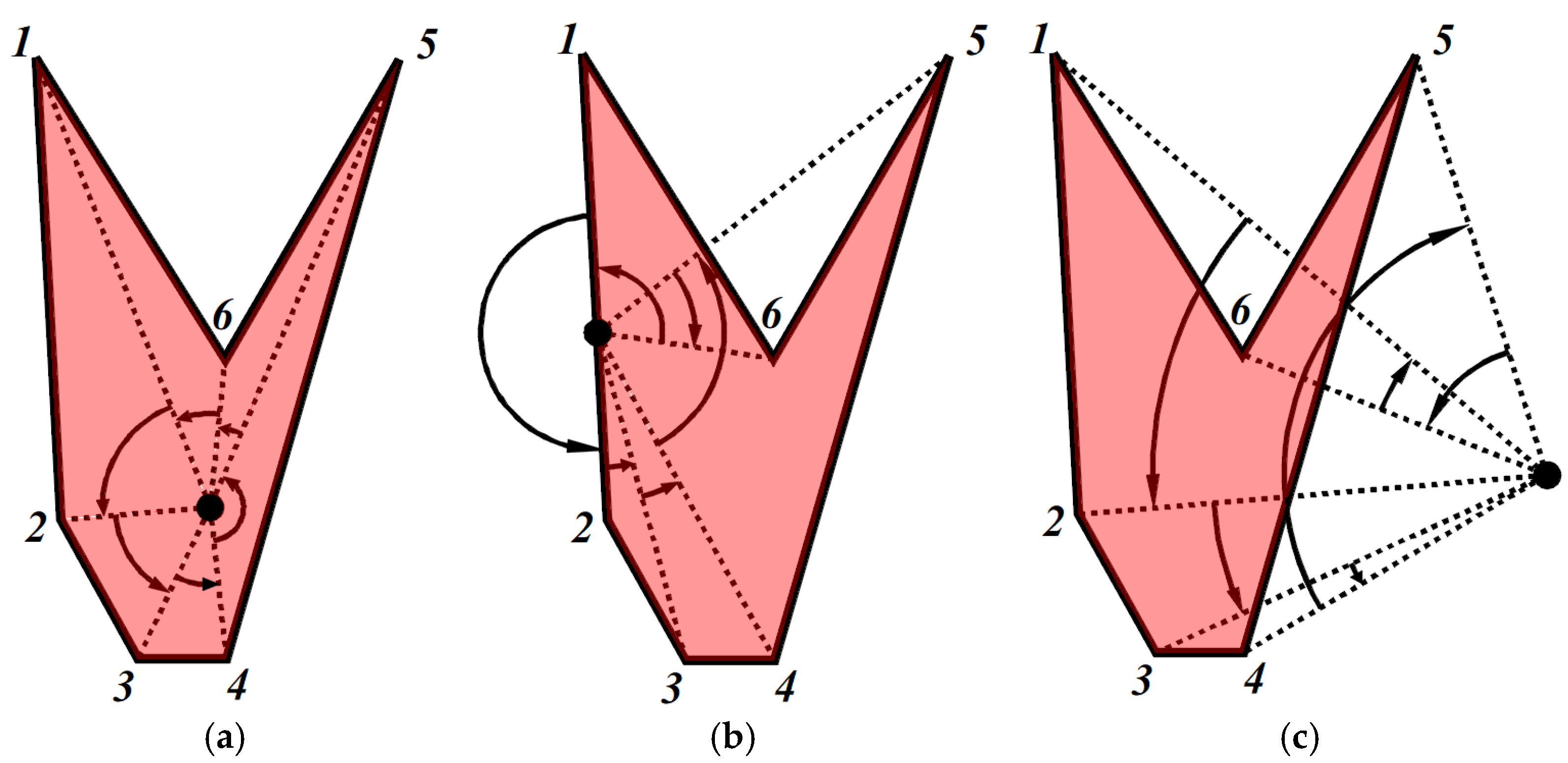
- similarly, find the entrance blocks of A to other vertexes of B. Combine them and E(A(2), B(0)1) to form E(A(2), B(0)), see Figure 5c;
- (4)
- (5)
- similarly, find the entrance blocks of other vertexes of A to B. Combine them and E(A(0)1, B(2)) to form E(A(0), B(2)), see Figure 5e;
- (6)
- find the entrance block E(A(1)1–2, B(1)1–2) of the 1–2 edge of A to the 1–2 edge of B, see Figure 5f;
- (7)
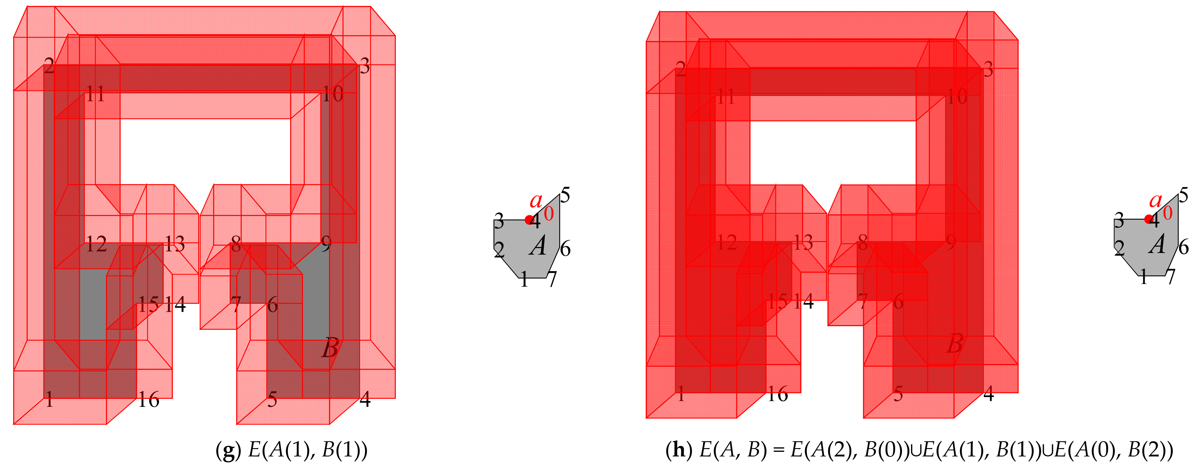
- similarly, find the entrance blocks of other edges of A to other edges of B. Combine them and E(A(1)1–2, B(1)1–2) to form E(A(1), B(1)), see Figure 5g;
- (8)
2.4. A Method to Reduce the Time Complexity of Entrance Block
3. A 2D Collision Detection Algorithm
- (1)
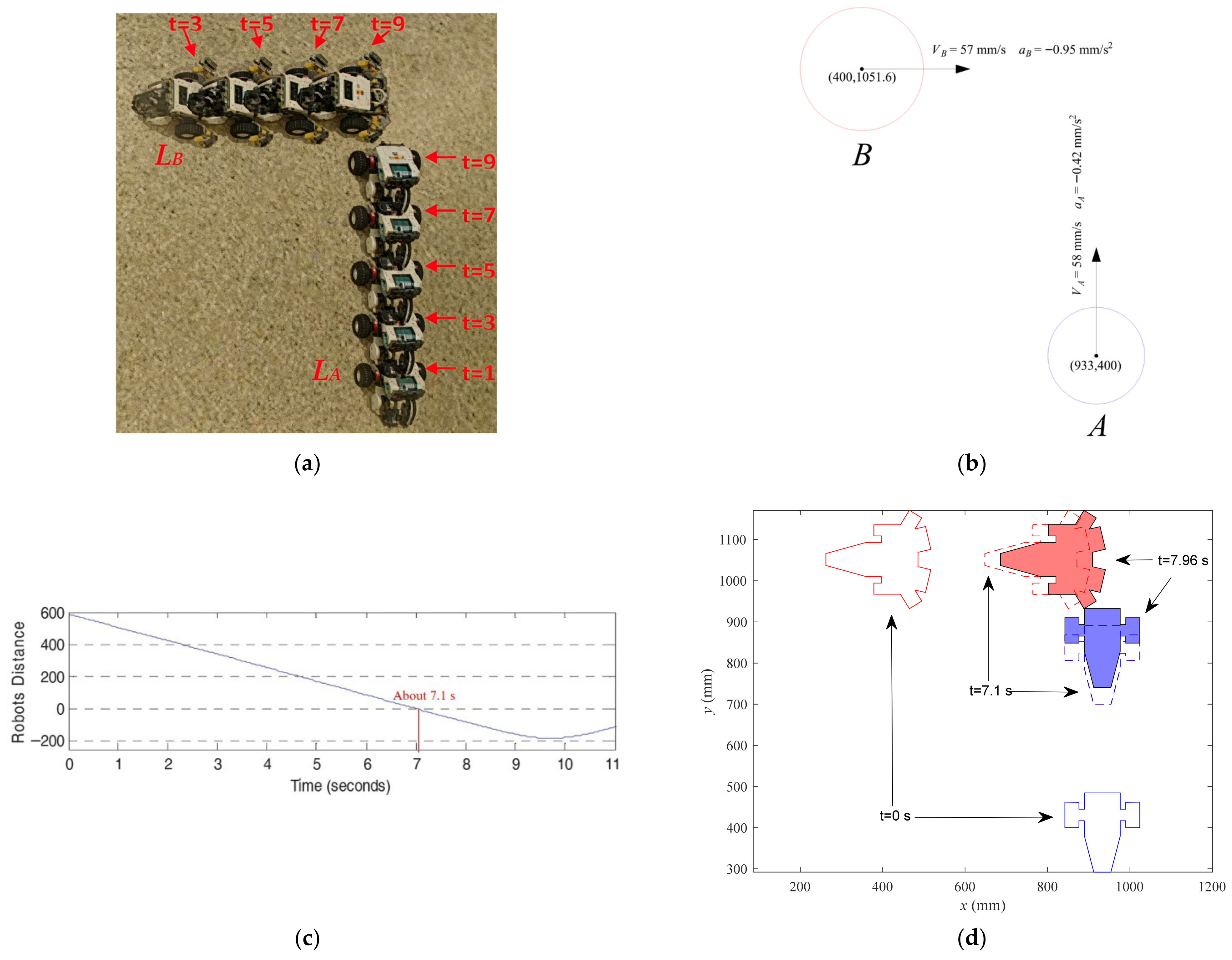
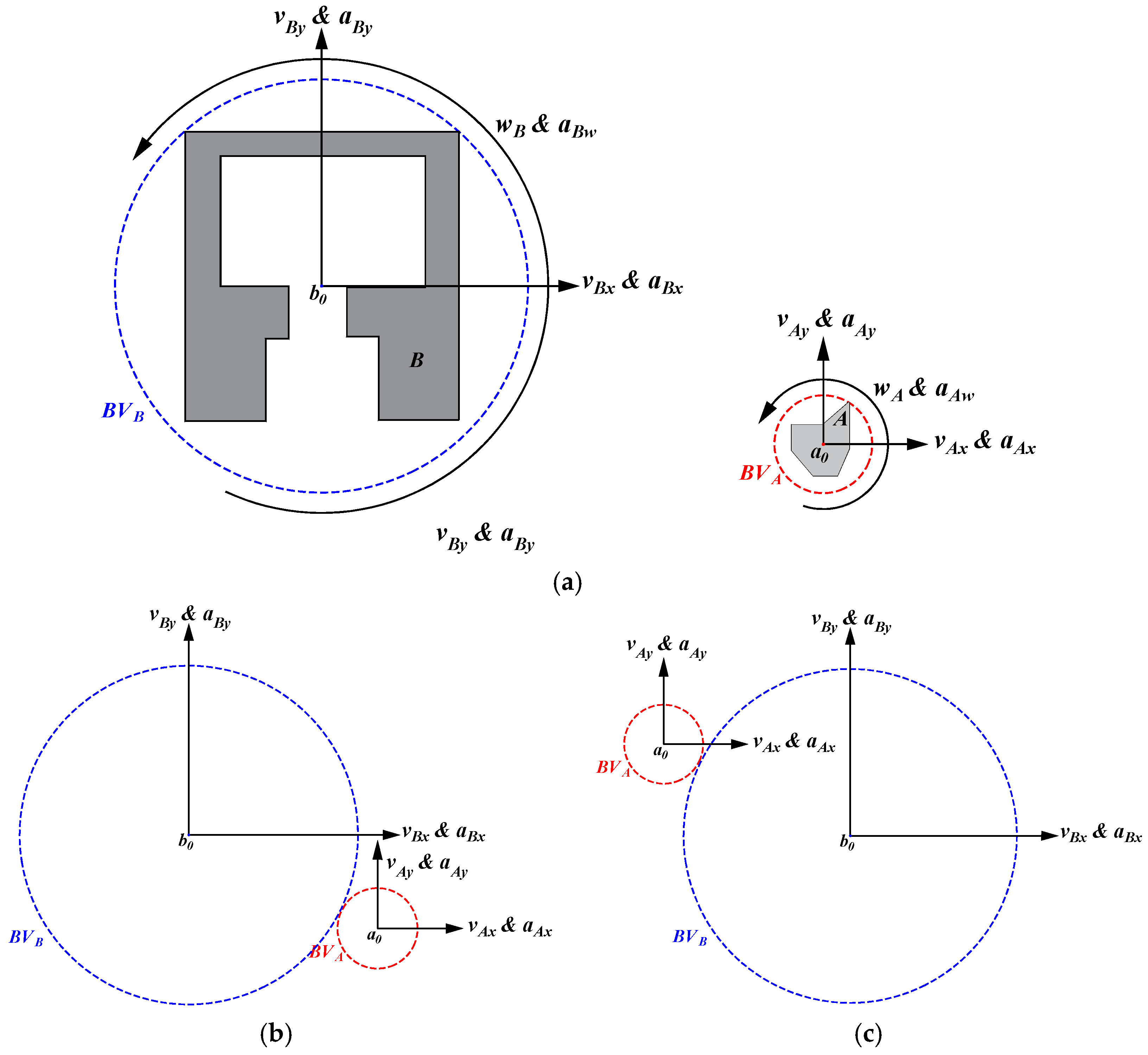
- calculate the maximum distance LA between the center of gravity a0 (xa0, ya0) and all vertexes of A. With a0 as the center, LA as the radius to make the bounding volume ball BVA of A. In the same way, make the bounding volume ball BVB of B, As shown in Figure 7a. Note that when the material of an object is uniform, its center of gravity is its centroid. The centroid of an arbitrary polygon can be calculated as follows [40]:where, Cx is the x coordinate of the centroid of the polygon; Cy is the y coordinate of the centroid of the polygon; n is the number of vertexes of the polygon; xi and yi are the x and y coordinates of the ith vertex of the polygon, respectively; xn+1 = x1 and yn+1 = y1.
- (2)
- solve the following Equation (5) for time (T). If A and B are likely to collide, the following Equation (5) for time (T) must have two positive real roots T1 and T2 (T2 > T1), as shown in Figure 7b,c. Otherwise, A and B would not collide.where, (xa0, ya0) and (xb0, yb0) are the coordinates of a0 and b0, respectively; vAx and vBx are the velocities in the x direction of A and B, respectively; vAy and vBy are the velocities in the y direction of A and B, respectively; aAx and aBx are the accelerations in the x direction of A and B, respectively; aAy and aBy are the accelerations in the y direction of A and B, respectively; LA and LB are the maximum distances between the centers of gravity a0 and b0 of A and B and their vertexes, respectively.
- (3)
- divide the time [T1, T2] equally produces n time points t1, t2, t3, …, and tn (t1 = T1 and tn = T2). Calculate the vertex positions of A and B at the n time points respectively.
- (4)
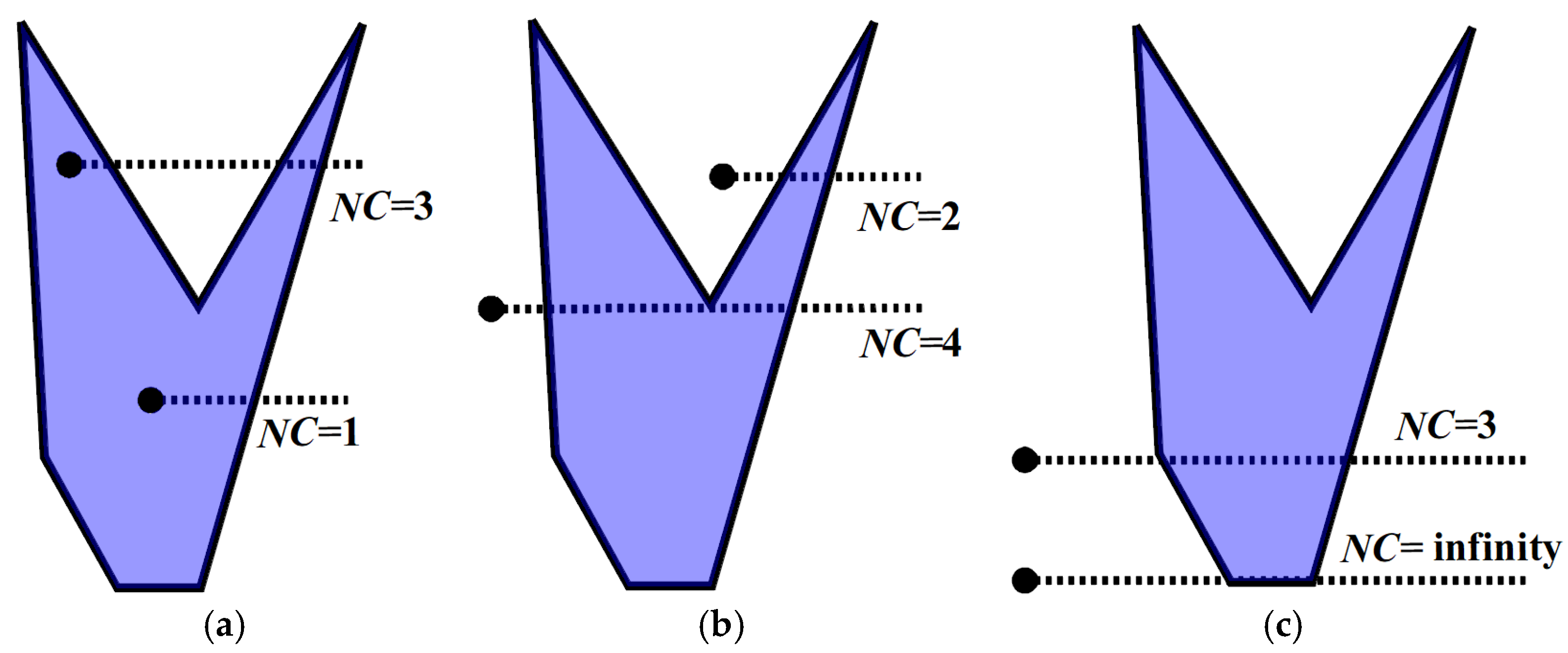
- for every time point, taking a0 as the reference point of A, calculate E(A(0), B(2)), E(A(2), B(0)), and E(A(1), B(1)) between A and B as described in Section 2. Judge the position relation of E(A(0), B(2)), E(A(2), B(0)) and E(A(1), B(1)) to a0 in turn. If a0 is inside E(A(0), B(2)) or E(A(2), B(0)) or E(A(1), B(1)), B(0)), it means that A and B have already collided at this time point. Otherwise, A and B have not collided.
- (5)
- find the first time point t0 when A and B overlap each other from all time points. Reset T1 to t0 − (T2 − T1)/n and reset T2 to t0.
- (6)
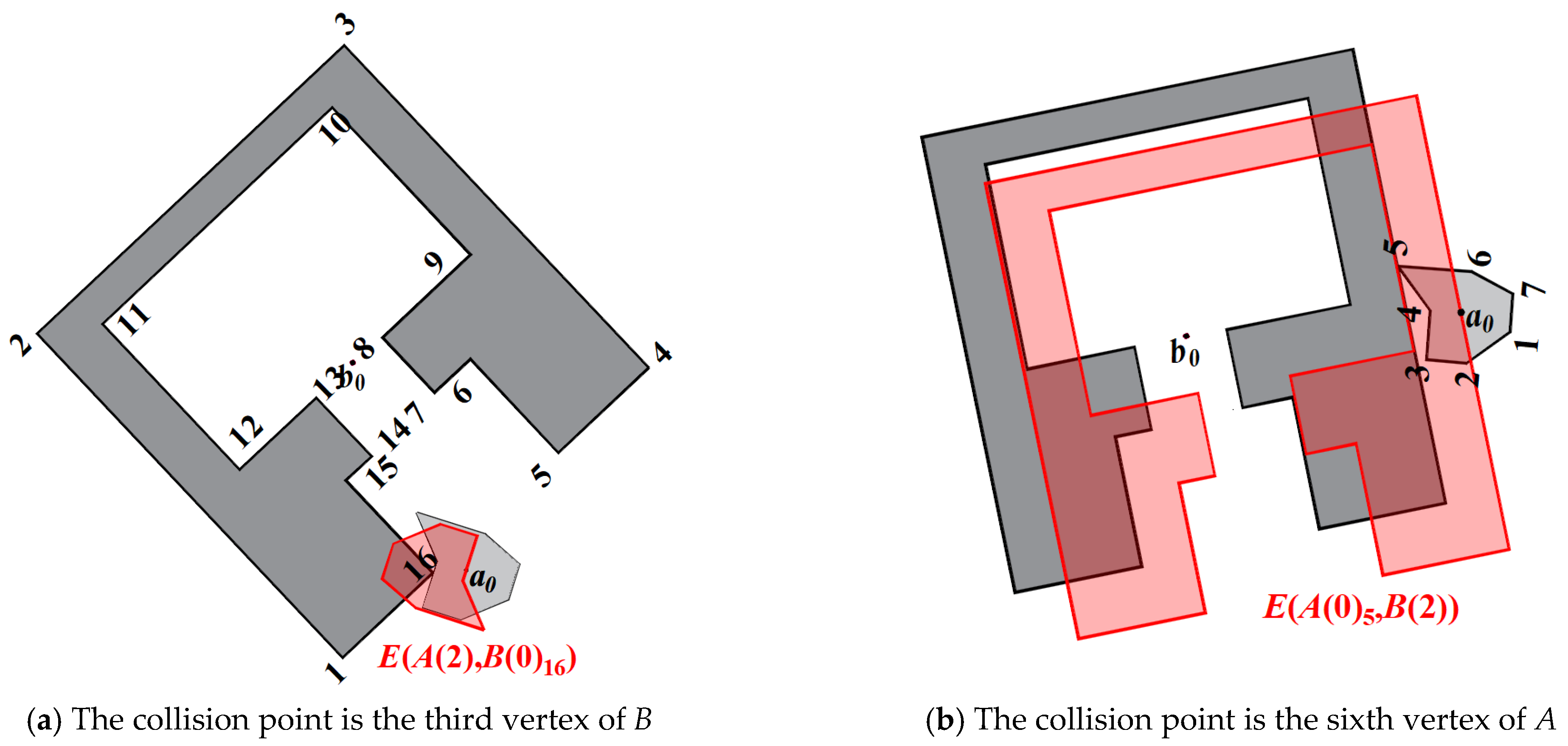
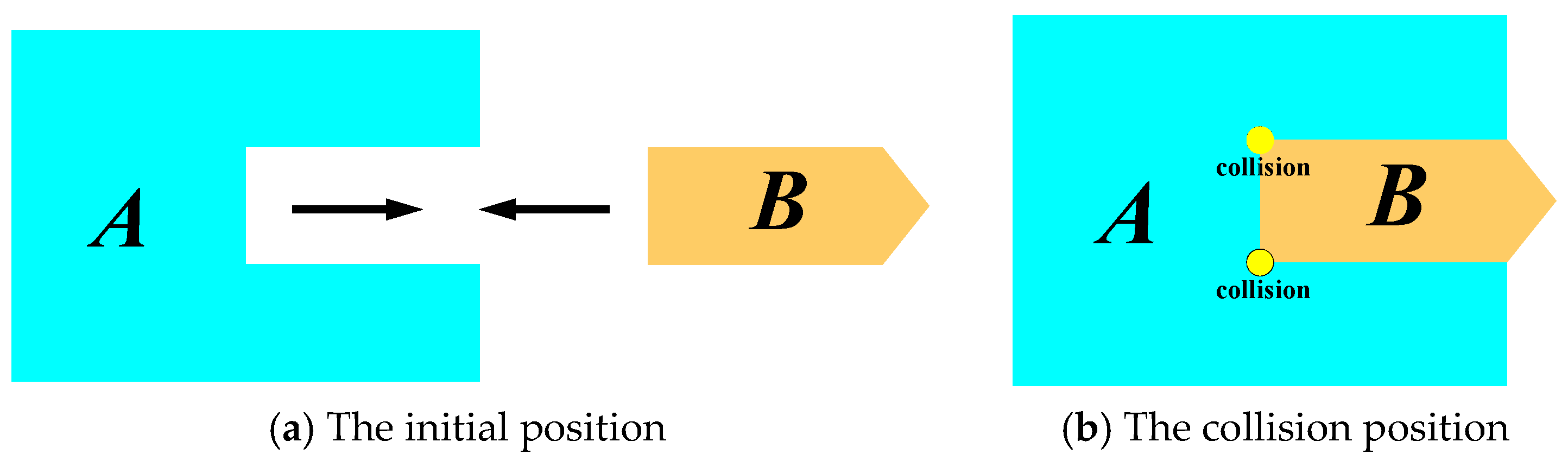
- repeat steps (3–4) until T2 − T1 < Threshold. T2 is the collision time between A and B. Recorded these E(A(0), B(2)) or E(A(2), B(0)) contains a0 in T2. The vertexes corresponding to these E(A(0), B(2)) or E(A(2), B(0)) containing a0 are the collision points between A and B. For example, if E(A(2), B(0)16) contains a0, the 16th vertex of B collides with A as shown in Figure 10a; if E(A(0)5, B(2)) contains a0, the 5th vertex of A collides with B as shown in Figure 10b. The initial interval [T1, T2] is obtained from the overlap condition of the two bounding volume balls and provides a conservative possible collision interval. During the refinement process, if t0 is the first sampled time point at which overlap is detected, the first collision time must lie between t0 and the previous sampled time point. Therefore, the interval is updated to . Since each refinement reduces the interval length to of the previous length, the interval converges as the refinement proceeds. The threshold is used as the stopping criterion and controls the temporal accuracy of the detected collision time. A smaller threshold improves accuracy but increases the number of refinement iterations, whereas a larger threshold improves efficiency but reduces accuracy.
4. Case
- (1)
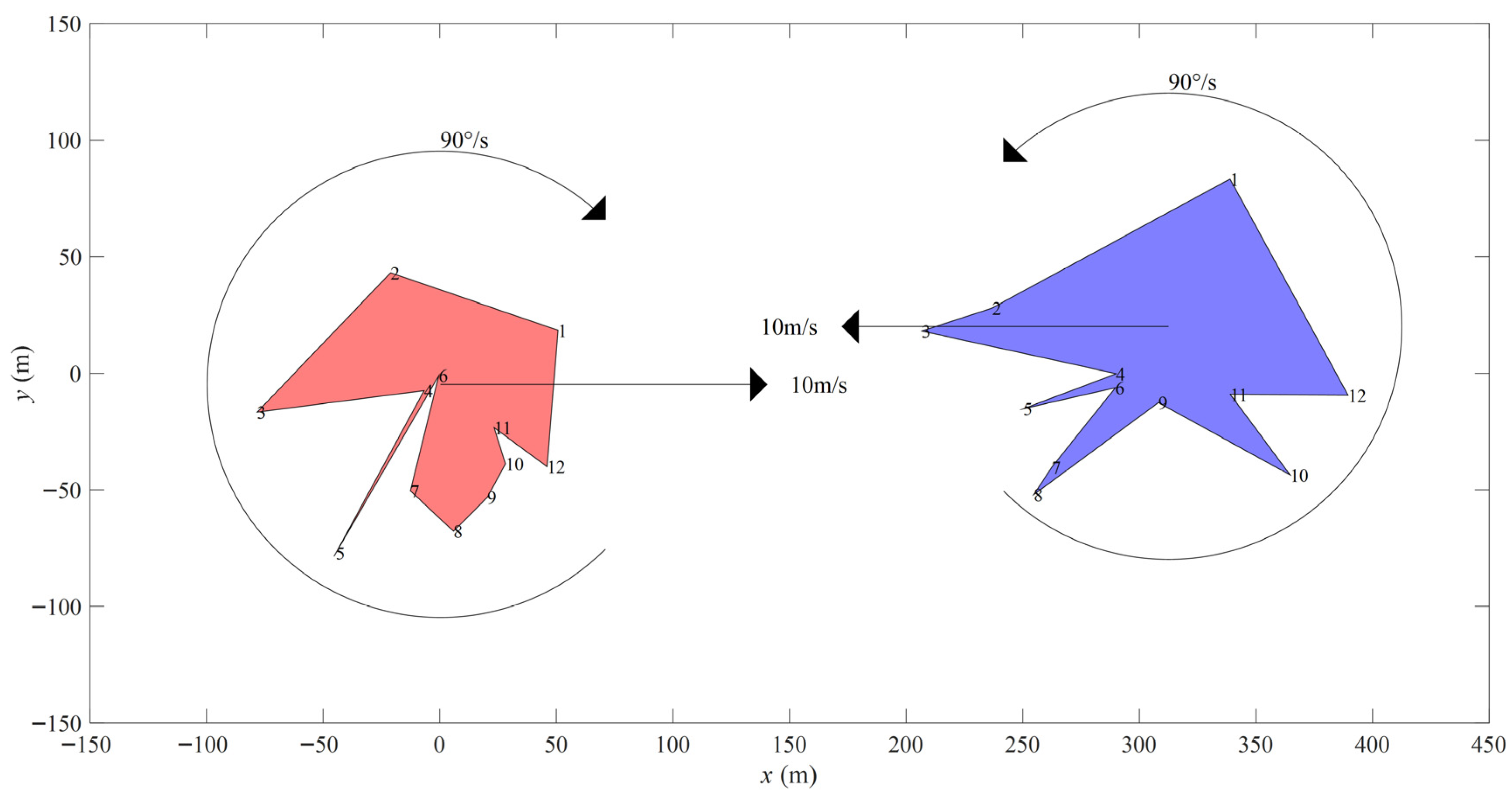
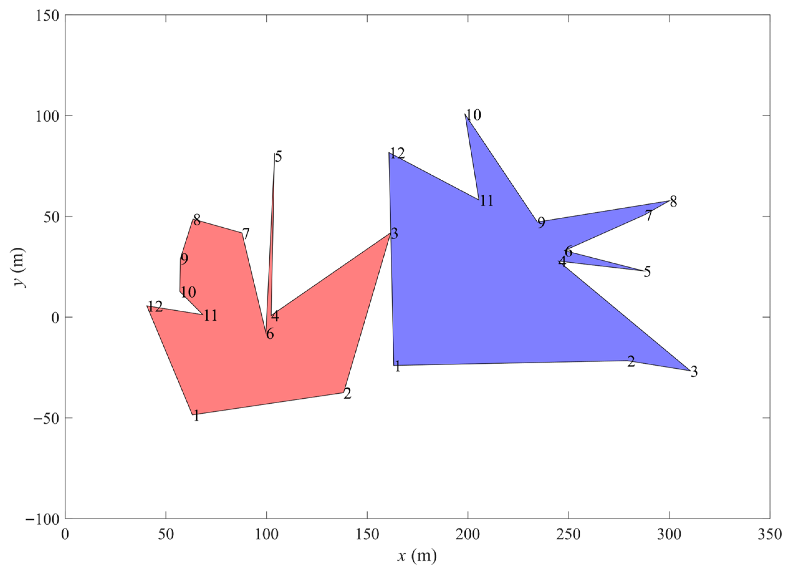
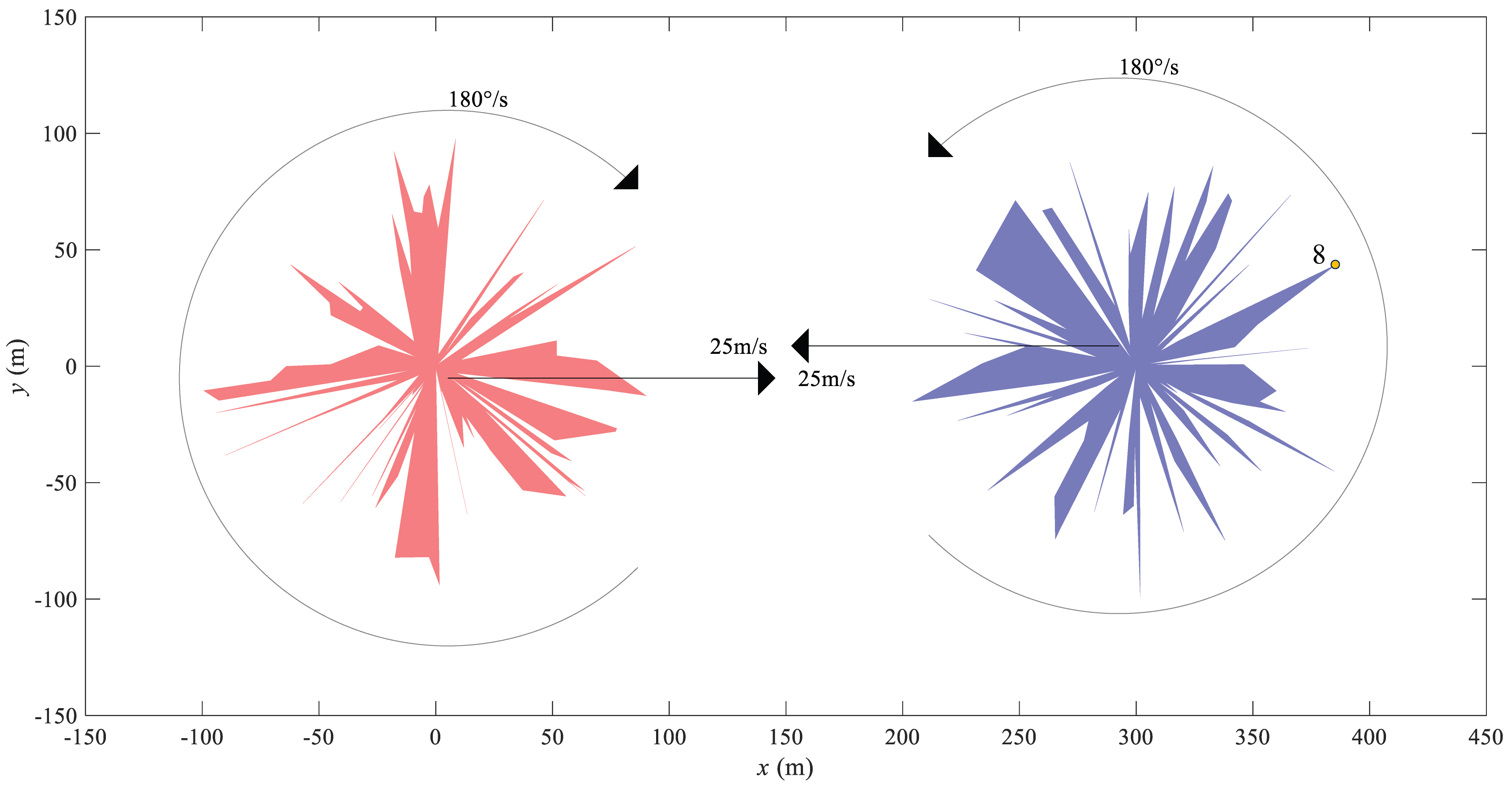
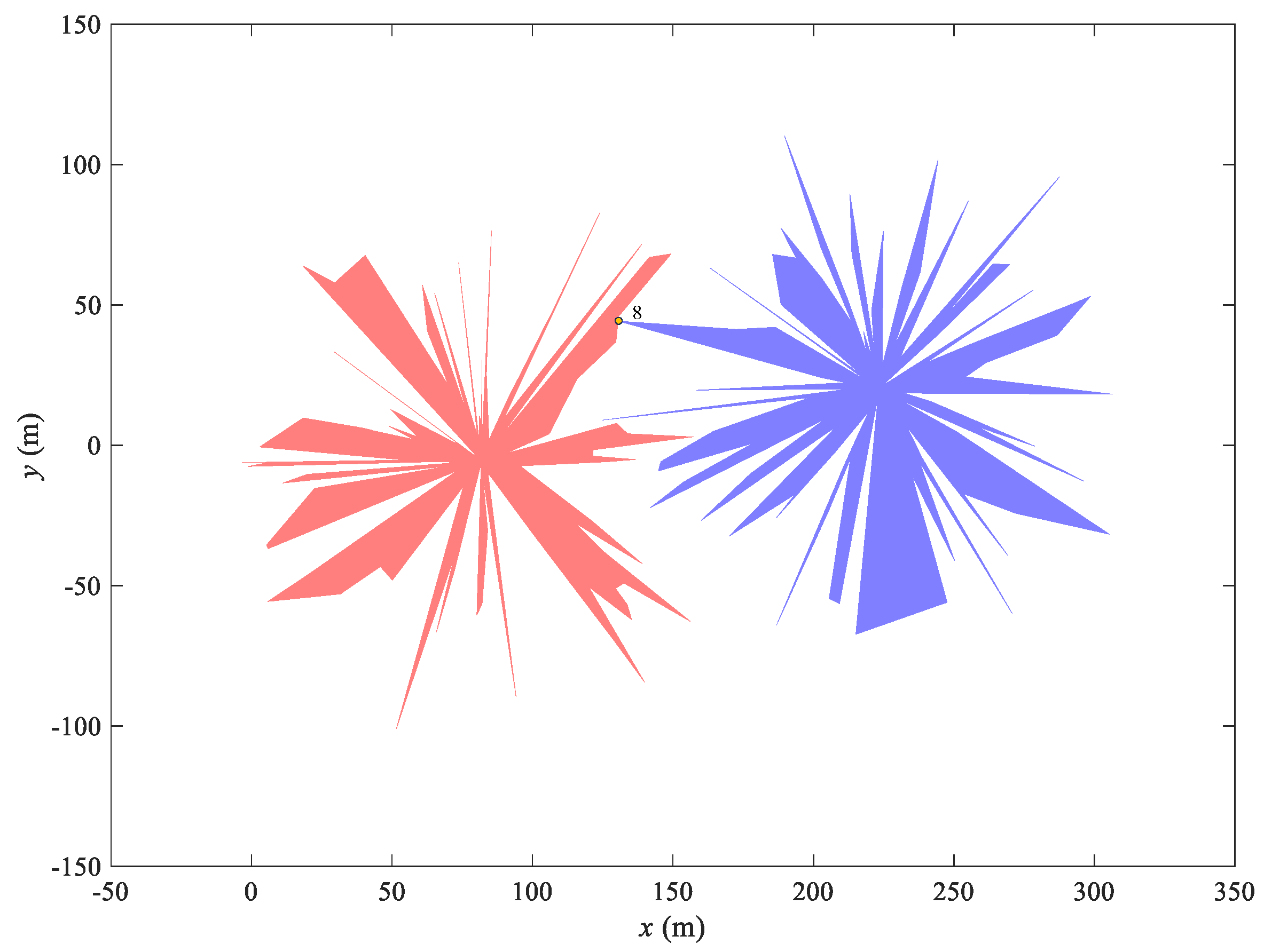
- Generates n random integers L = [l1, l2, …, ln] in [0 m, 100 m].
- (2)
- Generates n random integers θ = [θ1, θ2, …, θn] in [0°, 360°], and reorders θ from smallest to largest.
- (3)
- Use L and θ to calculate the vertex coordinates of the 2D object as follows:xj = ljcos(θj)where, xj is the x coordinate of the jth vertex of the 2D object; yj is the y coordinate of the jth vertex of the 2D object; lj is the jth integer in L; θj is the jth integer in θ.yj = ljsin(θj)
5. Discussion
- (1)
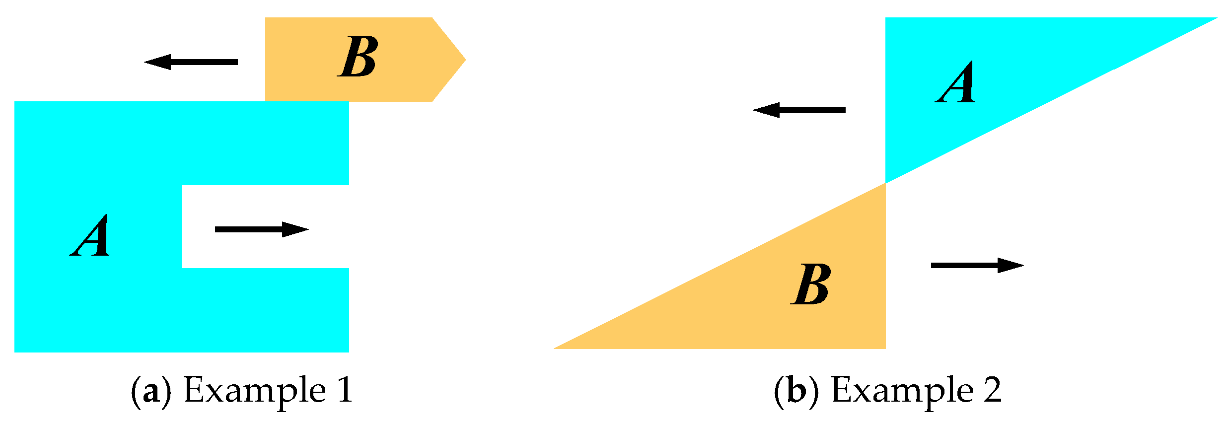
- Difference between collision and contact
- (2)
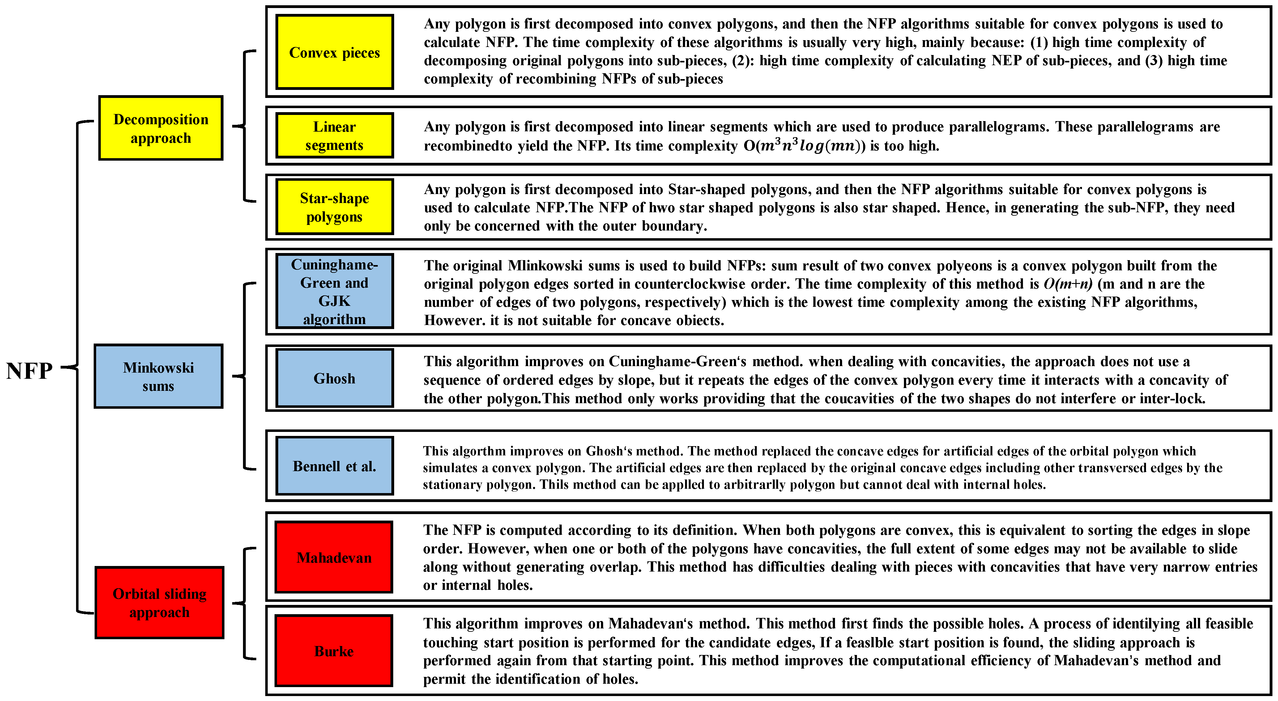
- Comparison with mainstream NFP-related algorithms for concave polygons
- (3)
- Potential of this discrete algorithm to evolve into a continuous algorithm
- (4)
- Potential of using entrance block for 3D collision detection
- (5)
- Applicability to objects with inner holes
- (6)
- Extension of ‘theorem of finite covers of entrance surfaces’ in 2D and its influence on NFP
6. Conclusions
Author Contributions
Funding
Data Availability Statement
Conflicts of Interest
Appendix A

| Red Object | Blue Object | ||||
|---|---|---|---|---|---|
| Vertex # | x Coordinate | y Coordinate | Vertex # | x Coordinate | y Coordinate |
| 1 | 50.74 | 18.47 | 1 | 338.88 | 83.38 |
| 2 | −21.04 | 43.14 | 2 | 236.97 | 28.06 |
| 3 | −78.25 | −16.63 | 3 | 206.75 | 18.13 |
| 4 | −6.69 | −7.43 | 4 | 290.00 | −0.17 |
| 5 | −44.50 | −77.08 | 5 | 250.27 | −15.20 |
| 6 | −0.37 | −0.93 | 6 | 289.71 | −6.18 |
| 7 | −12.58 | −50.46 | 7 | 262.49 | −40.22 |
| 8 | 5.93 | −67.74 | 8 | 254.73 | −52.07 |
| 9 | 20.43 | −53.21 | 9 | 308.17 | −12.58 |
| 10 | 28.21 | −38.83 | 10 | 364.66 | −43.62 |
| 11 | 23.33 | −23.33 | 11 | 338.97 | −9.00 |
| 12 | 46.04 | −40.02 | 12 | 389.51 | −9.41 |
| Red Object | Blue Object | ||||
|---|---|---|---|---|---|
| Vertex # | x Coordinate | y Coordinate | Vertex # | x Coordinate | y Coordinate |
| 1 | 68.96 | 2.41 | 1 | 345.99 | 0.80 |
| 2 | 51.80 | 4.53 | 2 | 307.98 | 0.56 |
| 3 | 51.84 | 11.02 | 3 | 324.86 | 2.61 |
| 4 | 10.67 | 2.66 | 4 | 373.59 | 7.74 |
| 5 | 85.72 | 51.50 | 5 | 304.91 | 0.95 |
| 6 | 30.19 | 19.61 | 6 | 342.21 | 8.20 |
| 7 | 52.23 | 35.23 | 7 | 352.00 | 17.91 |
| 8 | 32.77 | 22.94 | 8 | 385.54 | 43.58 |
| 9 | 0.69 | 0.72 | 9 | 318.00 | 10.82 |
| 10 | 37.51 | 40.22 | 10 | 310.18 | 6.36 |
| 11 | 33.46 | 38.49 | 11 | 348.30 | 43.49 |
| 12 | 14.69 | 20.23 | 12 | 308.04 | 7.50 |
| 13 | 2.87 | 4.10 | 13 | 366.24 | 73.57 |
| 14 | 46.29 | 71.29 | 14 | 316.40 | 18.87 |
| 15 | 1.04 | 4.89 | 15 | 334.11 | 50.57 |
| 16 | 3.34 | 31.82 | 16 | 341.00 | 71.01 |
| 17 | 6.89 | 78.70 | 17 | 339.44 | 74.17 |
| 18 | 8.54 | 97.63 | 18 | 320.71 | 44.41 |
| 19 | 1.03 | 58.99 | 19 | 330.09 | 70.88 |
| 20 | −2.72 | 77.95 | 20 | 332.97 | 85.89 |
| 21 | −5.09 | 72.82 | 21 | 332.61 | 84.96 |
| 22 | −5.75 | 65.75 | 22 | 307.16 | 20.80 |
| 23 | −9.32 | 66.35 | 23 | 314.24 | 53.13 |
| 24 | −17.94 | 92.27 | 24 | 316.43 | 77.27 |
| 25 | −11.23 | 52.82 | 25 | 302.44 | 19.85 |
| 26 | −10.35 | 38.64 | 26 | 305.23 | 74.82 |
| 27 | −18.74 | 65.37 | 27 | 297.49 | 47.93 |
| 28 | −15.39 | 42.29 | 28 | 296.91 | 58.92 |
| 29 | −9.18 | 10.57 | 29 | 296.71 | 26.80 |
| 30 | −32.70 | 29.44 | 30 | 297.37 | 8.61 |
| 31 | −41.51 | 36.08 | 31 | 291.23 | 28.69 |
| 32 | −31.09 | 25.17 | 32 | 271.57 | 87.50 |
| 33 | −32.36 | 23.51 | 33 | 284.37 | 45.38 |
| 34 | −62.26 | 43.59 | 34 | 291.21 | 25.53 |
| 35 | −45.43 | 27.30 | 35 | 263.85 | 67.99 |
| 36 | −44.94 | 21.92 | 36 | 259.83 | 66.86 |
| 37 | −8.16 | 3.80 | 37 | 298.41 | 2.54 |
| 38 | −24.43 | 8.89 | 38 | 248.27 | 71.19 |
| 39 | −44.99 | 0.79 | 39 | 231.43 | 41.20 |
| 40 | −64.00 | 0.00 | 40 | 270.86 | 15.49 |
| 41 | −70.73 | −6.19 | 41 | 239.28 | 28.32 |
| 42 | −99.45 | −10.45 | 42 | 271.81 | 10.26 |
| 43 | −92.84 | −14.70 | 43 | 211.55 | 28.74 |
| 44 | −9.88 | −1.56 | 44 | 272.27 | 8.48 |
| 45 | −93.90 | −19.96 | 45 | 283.44 | 3.82 |
| 46 | −15.97 | −5.81 | 46 | 226.38 | 14.31 |
| 47 | −90.21 | −38.29 | 47 | 252.73 | 8.34 |
| 48 | −55.23 | −23.44 | 48 | 234.01 | 1.15 |
| 49 | −22.66 | −10.57 | 49 | 204.19 | −15.17 |
| 50 | −7.06 | −3.76 | 50 | 268.70 | −6.65 |
| 51 | −21.92 | −21.92 | 51 | 292.17 | −1.66 |
| 52 | −56.96 | −58.99 | 52 | 223.50 | −23.39 |
| 53 | −5.56 | −5.75 | 53 | 265.23 | −12.65 |
| 54 | −24.09 | −26.75 | 54 | 244.92 | −21.14 |
| 55 | −9.37 | −10.40 | 55 | 283.07 | −8.63 |
| 56 | −10.07 | −12.43 | 56 | 293.14 | −4.12 |
| 57 | −4.11 | −5.66 | 57 | 286.89 | −9.18 |
| 58 | −40.72 | −58.16 | 58 | 236.42 | −53.35 |
| 59 | −4.90 | −7.55 | 59 | 279.66 | −23.40 |
| 60 | −27.18 | −55.73 | 60 | 277.63 | −31.95 |
| 61 | −7.61 | −16.31 | 61 | 265.03 | −55.97 |
| 62 | −25.79 | −60.75 | 62 | 265.35 | −74.32 |
| 63 | −16.28 | −47.28 | 63 | 267.46 | −69.79 |
| 64 | −8.96 | −27.58 | 64 | 285.15 | −34.98 |
| 65 | −17.46 | −82.16 | 65 | 293.50 | −17.85 |
| 66 | −2.86 | −81.95 | 66 | 282.08 | −62.48 |
| 67 | 1.64 | −93.99 | 67 | 299.88 | −0.99 |
| 68 | 0.09 | −1.00 | 68 | 296.97 | −28.84 |
| 69 | 13.51 | −63.58 | 69 | 294.42 | −63.76 |
| 70 | 0.21 | −0.98 | 70 | 298.95 | −59.99 |
| 71 | 2.47 | −10.72 | 71 | 299.42 | −32.99 |
| 72 | 2.66 | −10.67 | 72 | 301.73 | −98.98 |
| 73 | 12.05 | −34.98 | 73 | 301.58 | −12.90 |
| 74 | 11.27 | −21.19 | 74 | 320.40 | −71.13 |
| 75 | 16.43 | −30.90 | 75 | 305.99 | −14.83 |
| 76 | 12.88 | −21.43 | 76 | 316.48 | −40.80 |
| 77 | 21.24 | −32.71 | 77 | 338.14 | −74.84 |
| 78 | 23.42 | −36.06 | 78 | 317.45 | −31.49 |
| 79 | 37.28 | −53.24 | 79 | 304.47 | −6.63 |
| 80 | 55.86 | −55.86 | 80 | 336.00 | −42.90 |
| 81 | 20.06 | −18.07 | 81 | 320.48 | −19.10 |
| 82 | 64.15 | −55.77 | 82 | 310.57 | −9.18 |
| 83 | 56.60 | −49.20 | 83 | 353.62 | −45.00 |
| 84 | 63.58 | −53.35 | 84 | 339.13 | −29.49 |
| 85 | 14.55 | −12.21 | 85 | 315.37 | −11.17 |
| 86 | 5.59 | −4.21 | 86 | 309.01 | −6.31 |
| 87 | 49.52 | −37.31 | 87 | 317.61 | −11.44 |
| 88 | 58.16 | −40.72 | 88 | 312.24 | −6.79 |
| 89 | 10.18 | −6.36 | 89 | 328.86 | −16.00 |
| 90 | 8.48 | −5.30 | 90 | 384.76 | −45.07 |
| 91 | 50.88 | −31.80 | 91 | 348.53 | −23.67 |
| 92 | 77.05 | −28.05 | 92 | 322.47 | −10.96 |
| 93 | 77.53 | −26.70 | 93 | 341.08 | −15.77 |
| 94 | 8.51 | −2.93 | 94 | 364.07 | −19.59 |
| 95 | 73.28 | −10.30 | 95 | 352.87 | −15.16 |
| 96 | 90.11 | −12.66 | 96 | 360.07 | −10.59 |
References
- Franquesa, M.; Brunet, P. Collision Detection: Models and Algorithms. 1998, pp. 1–30. Available online: http://hdl.handle.net/2117/96814 (accessed on 22 March 2026).
- Kockara, S.; Halic, T.; Iqbal, K.; Bayrak, C.; Rowe, R. Collision detection: A survey. In Proceedings of the 2007 IEEE International Conference on Systems, Man and Cybernetics, Montreal, QC, Canada, 7–10 October 2007; pp. 4046–4051. [Google Scholar] [CrossRef]
- Zhang, X.; Lee, M.; Kim, Y.J. Interactive continuous collision detection for non-convex polyhedral. Vis. Comput. 2006, 22, 749–760. [Google Scholar] [CrossRef]
- Liao, X.; Lu, J.; Ma, J.; Xue, J.; Yu, X. Modeling of 2D Layout Design System Based on Convex Hull Plus Rubber Band Analog. Appl. Mech. Mater. 2012, 215–216, 1219–1223. [Google Scholar] [CrossRef]
- Zhang, D.; Yuen, M.M.F. A Coherence-based Collision Detection Method for Dressed Human Simulation. Comput. Graph. Forum 2002, 21, 33–42. [Google Scholar] [CrossRef]
- Huang, S.; Huang, L.; Lai, Z. An extension of the Fourier series-based particle model to the GJK-based contact detection and resolution framework for DEM. Comput. Part. Mech. 2022, 9, 381–391. [Google Scholar] [CrossRef]
- Kheradmand, E.; Laforest, M.; Prudhomme, S. A mathematical framework for the analysis and comparison of contact detection methods for ellipses and ellipsoids. Comput. Part. Mech. 2022, 9, 1153–1203. [Google Scholar] [CrossRef] [PubMed]
- Krijgsman, D.; Ogarko, V.; Luding, S. Optimal parameters for a hierarchical grid data structure for contact detection in arbitrarily polydisperse particle systems. Comput. Part. Mech. 2014, 1, 357–372. [Google Scholar] [CrossRef]
- Rubio-Largo, S.M.; Lind, P.G.; Maza, D.; Hidalgo, R.C. Granular gas of ellipsoids: Analytical collision detection implemented on GPUs. Comput. Part. Mech. 2015, 2, 127–138. [Google Scholar] [CrossRef]
- Shellshear, E. 1D sweep-and-prune self-collision detection for deforming cables. Vis. Comput. 2014, 30, 553–564. [Google Scholar] [CrossRef]
- Zheng, J.; Guo, J.; Wang, J.; Sun, H.; Deng, J.; Lü, Q. A universal elliptical disc (UED) model to represent natural rock fractures. Int. J. Min. Sci. Technol. 2022, 32, 261–270. [Google Scholar] [CrossRef]
- Guo, J.; Zheng, J.; Lü, Q.; Deng, J. Estimation of fracture size and azimuth in the universal elliptical disc model based on trace information. J. Rock Mech. Geotech. Eng. 2022, 15, 1391–1405. [Google Scholar] [CrossRef]
- Moore, M.; Wilhelms, J. Collision Detection and Response for Computer Animation. ACM SIGGRAPH Comput. Graph. 1988, 22, 289–298. [Google Scholar] [CrossRef]
- Hubbard, P.M. Interactive collision detection. In Proceedings of the 1993 IEEE Research Properties in Virtual Reality Symposium, San Jose, CA, USA, 25–26 October 1993; pp. 24–31. [Google Scholar] [CrossRef]
- Wang, M.; Cao, J. A review of collision detection for deformable objects. Comput. Animat. Virtual Worlds 2021, 32, e1987. [Google Scholar] [CrossRef]
- Teschner, M.; Kimmerle, S.; Heidelberger, B.; Zachmann, G.; Raghupathi, L.; Fuhrmann, A.; Cani, M.P.; Faure, F.; Magnenat-Thalmann, N.; Strasser, W.; et al. Collision Detection for Deformable Objects. Comput. Graph. Forum 2005, 24, 61–81. [Google Scholar] [CrossRef]
- Kamat, V. A survey of techniques for simulation of dynamic collision detection and response. Comput. Graph. 1993, 17, 379–385. [Google Scholar] [CrossRef]
- Lin, M.; Manocha, D. Fast interference detection between geometric models. Vis. Comput. 1995, 11, 542–561. [Google Scholar] [CrossRef]
- Jiménez, P.; Thomas, F.; Torras, C. 3D collision detection: A survey. Comput. Graph. 2001, 25, 269–285. [Google Scholar] [CrossRef]
- Gilbert, E.; Johnson, D.; Keerthi, S. Procedure for Computing the Distance Between Complex Objects in Three-dimensional Space. IEEE J. Robot. Autom. 2002, 4, 193–203. [Google Scholar] [CrossRef] [PubMed]
- Bergen, G.V.D. Ray Casting Against General Convex Objects with Application to Continuous Collision Detection. 2004, pp. 1–17. Available online: http://dtecta.com/papers/jgt04raycast.pdf (accessed on 22 March 2026).
- Burke, E.K.; Hellier, R.; Kendall, G.; Whitwell, G. Complete and robust no-fit polygon generation for the irregular stock cutting problem. Eur. J. Oper. Res. 2007, 179, 27–49. [Google Scholar] [CrossRef]
- Shi, G. Contact theory. Sci. China Technol. Sci. 2015, 58, 1450–1496. [Google Scholar] [CrossRef]
- Shi, G. Contact theory and algorithm. Sci. China Technol. Sci. 2021, 64, 1775–1790. [Google Scholar] [CrossRef]
- Art, R.C. An Approach to the Two Dimensional Irregular Cutting Stock Problem. Ph.D. Thesis, Massachusetts Institute of Technology, Cambridge, MA, USA, 1966; pp. 1–28. [Google Scholar]
- Adamowicz, M.; Albano, A. Nesting two dimensional shapes in rectangular modules. Comput. Aided Des. 1976, 8, 27–33. [Google Scholar] [CrossRef]
- Rocha, P. Robust NFP generation for Nesting problems. arXiv 2019, arXiv:1903.11139. [Google Scholar] [CrossRef]
- Ghosh, P.K. An algebra of polygons through the notion of negative shapes. CVGIP Image Underst. 1991, 54, 119–144. [Google Scholar] [CrossRef]
- Bennell, J.A.; Dowsland, K.A.; Dowsland, W.B. The irregular cutting-stock problem—A new procedure for deriving the no–fit polygon. Comput. Oper. Res. 2001, 28, 271–287. [Google Scholar] [CrossRef]
- Agarwal, P.K.; Flato, E.; Halperin, D. Polygon decomposition for efficient construction of Minkowski sums. Comput. Geom. 2002, 21, 39–61. [Google Scholar] [CrossRef]
- Avnaim, F.; Boissonnat, J.D. Polygon placement under translation and rotation. In Annual Symposium on Theoretical Aspects of Computer Science; Springer: Berlin/Heidelberg, Germany, 1988; Volume 294, pp. 323–333. [Google Scholar] [CrossRef]
- Li, Z.; Milenkovic, V.J. Compaction and separation algorithms for non-convex polygons and their applications. Eur. J. Oper. Res. 1995, 84, 539–561. [Google Scholar] [CrossRef]
- Mahadevan, A. Optimisation in Computer Aided Pattern Packing. Ph.D. Thesis, North Carolina State University, Raleigh, NC, USA, 1984. [Google Scholar]
- Bennell, J.A.; Song, X. A comprehensive and robust procedure for obtaining the nofit polygon using Minkowski sums. Comput. Oper. Res. 2008, 35, 267–281. [Google Scholar] [CrossRef]
- Zhuang, X.; Zheng, F.; Zheng, H.; Jiao, Y.; Rabczuk, T.; Wriggers, P. A cover-based contact detection approach for irregular convex polygons in discontinuous deformation analysis. Int. J. Numer. Anal. Methods Geomech. 2021, 45, 208–233. [Google Scholar] [CrossRef]
- Jiao, Y.; Zhao, Q.; Zheng, F.; Wang, L. Latest advances in discontinuous deformation analysis method. Sci. China Technol. Sci. 2017, 60, 963–964. [Google Scholar] [CrossRef][Green Version]
- Li, C.; Yang, Y.; Zheng, H. Numerical study of soil-rock mixture: Generation of random aggregate structure. Sci. China Technol. Sci. 2018, 61, 359–369. [Google Scholar] [CrossRef]
- Liu, Q.; Jiang, Y.; Jun, H. Precision improvement methods and research trends of discontinuous deformation analysis. Rock Soil Mech. 2017, 38, 1746–1761. [Google Scholar] [CrossRef]
- Wang, L.; Jiao, Y.; Huang, G.; Zheng, F.; Zhao, Z.; Tan, F. Improvement of contact calculation in spherical discontinuous deformation analysis. Sci. China Technol. Sci. 2017, 60, 765–771. [Google Scholar] [CrossRef]
- Robert, N. Calculating the Area and Centroid of a Polygon in 2d; Imperial College London: London, UK, 2013; Available online: https://www.ma.ic.ac.uk/~rn/centroid.pdf (accessed on 22 March 2026).
- Haines, E. Point in Polygon Strategies. Graph. Gems 1994, 4, 24–46. [Google Scholar] [CrossRef]
- Bernabeu, E.J.; Valera, A.; Gomez-Moreno, J. Distance Computation Between Non-Holonomic Motions with Constant Accelerations. Int. J. Adv. Robot. Syst. 2013, 10, 329. [Google Scholar] [CrossRef]
- An, H.; Jung, J.I. Design of a Cooperative Lane Change Protocol for a Connected and Automated Vehicle Based on an Estimation of the Communication Delay. Sensors 2018, 18, 3499. [Google Scholar] [CrossRef]
- Redon, S.; Kheddar, A.; Coquillart, S. Fast Continuous Collision Detection between Rigid Bodies. Comput. Graph. Forum 2002, 21, 280–287. [Google Scholar] [CrossRef]
- Keissar, Y.; Gardner, M.; Sitar, N. Benchmarking Contact Detection Algorithms Used in Polyhedral Particle System. Int. J. Numer. Anal. Methods Geomech. 2026, 50, 53–64. [Google Scholar] [CrossRef]
- Bennell, J.A.; Oliveira, J.F. The geometry of nesting problems: A tutorial. Eur. J. Oper. Res. 2008, 184, 397–415. [Google Scholar] [CrossRef]
- Min, T.; Curtis, S.; Sung-Eui, Y.; Manocha, D. ICCD: Interactive Continuous Collision Detection between Deformable Models Using Connectivity-Based Culling. IEEE Trans. Vis. Comput. Graph. 2009, 15, 544–557. [Google Scholar] [CrossRef] [PubMed]





| Symbols | Meaning |
|---|---|
| A | An arbitrary object |
| B | Another arbitrary object |
| a0 | The reference point of A(a0 may not belong to A) |
| E(A, B) | Entrance block of A to B |
| ∂E(A, B) | The boundary of the entrance block of A to B |
| E(A(2), B(0)i) | Entrance block of A to the ith vertex of B, when A is a 2D object |
| E(A(0)j, B(2)) | Entrance block of the jth vertex of A to B, when A is a 2D object |
| E(A(1)i-j, B(1)k-h) | Entrance block of the i-j edge of A to the k-h edge of B |
| E(A(1)i-j, B(1)) | Entrance block of the i-j edge of A to all edges of B |
| A(3) | A(3) is a 3D object |
| B(3) | B(3) is a 3D object |
| A(2) | A(2) = A, when A is a 2D object |
| B(2) | B(2) = B, when B is a 2D object |
| A(1) | A(1) is the boundary of A when A is a 2D object |
| B(1) | B(1) is the boundary of B when B is a 2D object |
| A(0) | A(0) is the point set that includes all vertexes of A |
| B(0) | B(0) is the point set that includes all vertexes of B |
| ∪ | Union calculation symbol |
| Method | Applicable Object Types | Concave Polygons and Holes | Treatment of Rotation | Computational Complexity/Feature | Main Limitations |
|---|---|---|---|---|---|
| Original Minkowski-sum/GJK-based methods | Mainly convex polygons | Not directly applicable to concave polygons or holes | Rotation can be considered only by repeated updating or sampling | Efficient for convex objects; original Minkowski-sum construction is usually O(m + n) | Not directly suitable for complex concave polygons |
| Improved Minkowski-sum methods | Convex and some concave polygons | Can handle concave polygons with extensions; holes depend on implementation | Usually not the main focus | Higher complexity due to Boolean operations and special treatments | Robustness and efficiency decrease for complex concavities and holes |
| Decomposition-based methods | Concave polygons after decomposition | Applicable after decomposing concave polygons; holes depend on decomposition strategy | Usually not the main focus | Usually high complexity due to decomposition, sub-NFP construction, and recombination | Efficiency strongly depends on decomposition quality |
| Orbital sliding methods | General polygons | Applicable to many concave polygons; holes and narrow concavities require special treatment | Usually not the main focus | No simple fixed complexity; cost depends on iterative sliding steps, contact events, and additional procedures for holes or feasible start positions | May fail or require extra procedures for narrow concavities, holes, and feasible starting positions |
| Proposed entrance-block-based method | Arbitrary 2D objects | Applicable to convex and concave objects; potentially applicable to objects with holes based on Contact Theory | Considered by time-discrete updating of object positions | Entrance block construction can be simplified from O(mn) to O(m + n) in this study | Current implementation is time-discrete and may suffer from tunneling |
Disclaimer/Publisher’s Note: The statements, opinions and data contained in all publications are solely those of the individual author(s) and contributor(s) and not of MDPI and/or the editor(s). MDPI and/or the editor(s) disclaim responsibility for any injury to people or property resulting from any ideas, methods, instructions or products referred to in the content. |
© 2026 by the authors. Licensee MDPI, Basel, Switzerland. This article is an open access article distributed under the terms and conditions of the Creative Commons Attribution (CC BY) license.
Share and Cite
Li, G.; Wang, J.; Dong, S.; Zhang, R. A Narrow-Phase Collision Detection Algorithm Based on Contact Theory in 2D. Mathematics 2026, 14, 1965. https://doi.org/10.3390/math14111965
Li G, Wang J, Dong S, Zhang R. A Narrow-Phase Collision Detection Algorithm Based on Contact Theory in 2D. Mathematics. 2026; 14(11):1965. https://doi.org/10.3390/math14111965
Chicago/Turabian StyleLi, Gen, Jiongchao Wang, Shihua Dong, and Ruichen Zhang. 2026. "A Narrow-Phase Collision Detection Algorithm Based on Contact Theory in 2D" Mathematics 14, no. 11: 1965. https://doi.org/10.3390/math14111965
APA StyleLi, G., Wang, J., Dong, S., & Zhang, R. (2026). A Narrow-Phase Collision Detection Algorithm Based on Contact Theory in 2D. Mathematics, 14(11), 1965. https://doi.org/10.3390/math14111965