Forced Nonlinear Vibration of an Axially Functionally Graded Beam Under the Combined Effects of Electromagnetic Actuation, Mechanical Impact, and Casimir Force

Abstract

The present study deals with the nonlinear forced vibration of an axially functionally graded beam subjected to an electromagnetic actuator, moving load, and Casimir force, considering the curvature of the beam and it resting on a nonlinear elastic Winkler–Pasternak foundation. The presence of an electromagnetic actuator and Casimir force besides the presence of mechanical impact (moving load) and nonlinear elastic foundation is a characteristic of a real system, but this has not been studied in this form until now, currently representing a remaining gap. The governing differential equations of motion in the considered system are based on Euler–Bernoulli beam theory and von Kármán geometric nonlinearity. The material properties are expressed according to a power law function through the thickness direction. We point out that the present study is the first to consider the curvature in combination with electromagnetic actuation, Casimir force, an elastic foundation, and moving load. Unlike in other works, axial inertia is not assumed to be negligible in our investigation. The Optimal Homotopy Asymptotic Method is employed to obtain an approximate analytical expression for the nonlinear dynamic response and the nonlinear frequency. The solutions obtained are very accurate in comparison with numerical solutions, and our procedure is simple and easy to implement for nonlinear problems. The local stability near the primary resonance and internal resonance is analyzed by means of the variable expansion method, the homotopy perturbation method, equilibrium points, the Jacobian matrix, and the Routh–Hurwitz criterion.

1. Introduction

Functionally graded materials are usually nonhomogeneous materials in which the volume fractions of two or more material constituents, such as ceramic and metal, are designed to vary continuously as a function of spatial position along the desired directions. The structural dynamics and statics of these materials have been studied extensively in the last several years. Thomas et al. [1] employed a finite element modeling approach for free vibration analysis of FG nanocomposite beams reinforced by randomly oriented straight single-walled carbon nanotubes. The Eshelbiy–Mori–Tanaka approach based on equivalent fiber was used for the vibration of the Timoshenko beam. Vo et al. [2] presented a static and vibration analysis of functionally graded beams (FGBs) using refined shear deformation theory; a two-nod Hermite-cubic element with five degrees of freedom per mode was developed to solve the problem.

Zenkour and Abouelregal [3] examined the effect of two temperatures in FG nanobeams with harmonically varying heat. Their model was based upon Green and Naghdi’s theory as well as on the nonlocal thin beam theory. The inverse Laplace transform and the Fourier series expansion technique were used in this problem. Ebrahimi and Moktari [4] studied the free vibration of a rotating Mori–Tanaka-based FGB; Timoshenko beam theory and the differential transform method were employed to find the solution to the free vibration. The behavior of an exponentially graded hybrid cylindrical shell subjected to an axisymmetric thermo-electro-mechanical loading in a constant magnetic field was explored by Saadatfar and Khafri [5] who used Fourier series expansion and the differential quadrature method to obtain a numerical solution. The coupled longitudinal–transverse–rotational free vibration behavior of post-buckled FG micro- and nano-beams based on Mindlin strain gradient theory was investigated by Ansari et al. [6]. A first-order shear deformable beam model and von Kármán geometric nonlinearity were developed, and the generalized differential quadrature method was derived to numerically solve them via Newton’s method.

The fundamental frequency of sandwich beams with FG face sheets and homogeneous cores was explored by Ma and Zhao [7]. The classical plate theory and a higher-order theory were used to analyze the core of the sandwich beams, considering both the transverse normal and shear strain of the core. The free and forced vibration of an FG Timoshenko beam in a thermal environment was proposed by Nguyen and Bui [8] using hierarchical functions to interpolate the kinematic variables and a higher-order finite beam element. The shear strain was kept constant to improve the efficiency of the element. Fan and Huang [9] examined the nonlinear vibration of carbon-nanotube-reinforced composite beams resting on a nonlinear elastic foundation in a thermal environment by means of a simple and effective approach based on the Haar wavelet discretization method.

An analytical treatment of the size-dependent nonlinear secondary resonance of FG porous materials micro/nano beams subjected to periodic hard excitations was employed by Fattahi et al. [10]. The mechanical properties of the FG porous materials micro-/nanobeams were explored based upon the closed-cell Gaussian random field scheme for three different FG porosity dispersion patterns. An explicit analytical expression for the nonlocal strain gradient frequency and amplitude responses was obtained using the multiple time scales method. Babaei et al. [11] established the governing equations for an arch with the aid of Reddy’s third-order shear deformation curved beam theory and von Kármán-type strain–displacement relations. The governing equations were solved by means of a two-step perturbation procedure for clamped–clamped FG material shallow arches. The nonlinear vibration of an axially FG beam resting on a nonlinear elastic foundation and subjected to a moving harmonic load was investigated by Alimoradzadeh et al. [12], utilizing Green’s strain tensor. The nonlinear frequency and nonlinear dynamic response were obtained using the variational iteration method. Shafiei et al. [13] considered the vibration of a rotary-tapered axially FG Timoshenko nanobeam in a thermal environment, based on non-local theory. The governing equations of motion were solved using the generalized differential quadrature element method.

Based on Euler–Bernoulli theory, Ma et al. [14] explored the electromechanical behavior of FG piezoelectric composite beams containing an axially FG beam and a piezoelectric actuator subjected to electrical load. The integration-by-parts procedure was utilized to solve the differential governing equation. The natural transverse vibration of an axially FG-tapered double embedded in an elastic medium was presented by Sari et al. [15]. Eringen’s non-local elasticity theory and Chebyshev’s spectral collocation method were applied to find the frequencies and mode shapes. The free vibration of axially FG double-tapered Timoshenko beams, obtained by applying nonuniform rational B-spline basis functions, was studied by Zhou et al. [16]. The proposed method leads to higher accuracy and better sharpness than the standard finite element method. The nonlinear forced vibration of an FG carbon-nanotube-reinforced composite beam resting on a nonlinear viscoelastic foundation and subjected to a transverse periodic excitation was investigated by Shafiei and Setoodeh [17]. Four types of distributions through the thickness direction of the beam were considered, and the Eshelby–Mori–Tanaka approach was used to predict the effective material properties.

Hieu et al. [18] applied the non-local strain gradient beam model considering the thickness effect in the study of the nonlinear vibration response of an FG nanobeam. They pointed out that the effect of thickness is very important for the size-dependent vibration response of the nanobeam. Yas and Rahimi [19] considered the thermal vibration of FG porous nanocomposite beams reinforced by graphene platelets, considering variation in the Poisson ratio and the relation between the porosity coefficient and the mass density under a Gaussian random field. The governing equations were discretized and solved by means of the generalized differential quadrature method. A two-dimensional piezoelasticity-based analytical solution for free vibration of axially FG beams integrated with piezoelectric layers and subjected to arbitrary support boundary conditions was explored by Singh and Kumari [20]. To reduce the governing equation into ordinary differential equations along the axial and thickness directions, the extended Kantorovich method was employed, and benchmark numerical results were presented. Chen et al. [21] investigated the mechanical and electrical properties of FG flexo-piezoelectric beams under different electrical boundary conditions. The deflection and induced electric potential were given as analytical expressions for an FG cantilever beam. The geometrically nonlinear vibration of an FGB reinforced by surface-bounded piezoelectric fibers located on an arbitrary number of supports and subjected to excitation forces and thermoelectric changes was examined by Elkhouddar et al. [22]. The numerical results for a wide range of amplitudes were given using the approximate multimodal method close to the predominant mode.

Anh and Hieu [23] considered the nonlinear vibration response of the nonlocal strain gradient of single-walled carbon nanotubes under a magnetic field. An analytical form was given for the nonlinear frequencies of the considered model resting on an elastic foundation, under a longitudinal magnetic field using the equivalent linearization method with weighted averaging. Wu et al. [24] analyzed the nonlinear forced vibration of bidirectional FG porous material beams in which the material components’ gradient changes in both the thickness and axial directions. The vibration response curves were obtained using the max–min amplitude of periodic motions and via the pseudo-arc-length technique. The large deflection analysis of an FG-saturated porous rectangular plate subjected to transverse loading, located on a nonlinear three-parameter elastic foundation, was explored by Alhaifi et al. [25]. The constitutive law for the porous materials was based on Biot’s model, considering the effect of fluids within the pores, and the generalized differential quadrature method was applied to solve the nonlinear problem.

Dang and Nguyen [26] examined the buckling and nonlinear free vibration of FG porous micro-beams resting on an elastic foundation using the nonlocal strain gradient theory. Two porosity distribution models, including even and uneven distributions, were considered to emphasize the effect of porosity. Analytical solutions for the vibration of a bidirectional FG nanobeam were employed by Nazmul et al. [27]. Eringen’s non-local elasticity theory was followed to model the small-scale effects, and the nanobeam’s vibrational behavior was formulated by applying the Euler–Bernoulli and Timoshenko beam theories. It was shown that when the material parameter along the axis increases, clamped nanobeams have a higher natural frequency, while simply supported, cantilevered, and propped cantilevered nanobeams have a lower natural frequency.

Based on von Karman large deflection geometry and Reddy theory, Chang et al. [28] studied the internal resonance of FGM blade under centrifugal and aerodynamic forces. Recent advances were reported by Zang et al. in [29] on incorporating NiTiNOL–steel wire ropes as an efficient approach to nonlinear vibration control of FG beams and related structures. Nonlinear forced vibration in multi-physics and a coupled nonlinear modeling for composite cylindrical shell was analyzed by Liu et al. [30]. A wave approach is used by Abdi et al. [31] to study the forced vibrations of a rod with a nonlinear boundary stiffness under time-harmonic excitation. A numerical study is performed to determine the forced response, together with the region in which there are multiple solutions. The impulse vibration suppression performance of adjustable parallel nonlinear energy sinks with two repulsive magnets was investigated by Guo et al. [32] involving beams in bending. The dynamic model is proposed, and key absorber parameters are optimized.

The present study is devoted to nonlinear forced vibration of a clamped–clamped axially FGB, subjected to an electromagnetic actuator, moving load, and Casimir force, and resting on a nonlinear elastic Winkler–Pasternak foundation. The current study advances beyond all the above-mentioned achievements due to simultaneously considering all these aspects. The presence of an electromagnetic actuator and Casimir force besides the presence of moving load and nonlinear elastic foundation is a characteristic for a real system, but this has not been studied in this form until now, being currently a remaining gap. Also, for this complex system, an analytical solution with high accuracy is not known until now. The coupled longitudinal–transversal governing equations are discretized by means of the Galerkin–Bubnov procedure. The nonlinearity of the equations is due to the curvature of the beam and the electromagnetic actuator, Casimir force, and nonlinear foundation. The nonlinear differential equation is solved by means of the Optimal Homotopy Asymptotic Method (OHAM). A very accurate solution is obtained using a moderate number of auxiliary functions and convergence-control parameters. The effects of different parameters are presented. The local stability near the primary resonance is studied with the help of the variable expansion method and homotopy perturbation method using the equilibrium points, Jacobian matrix, and Routh–Hurwitz criterion.

2. Determining the Governing Equations

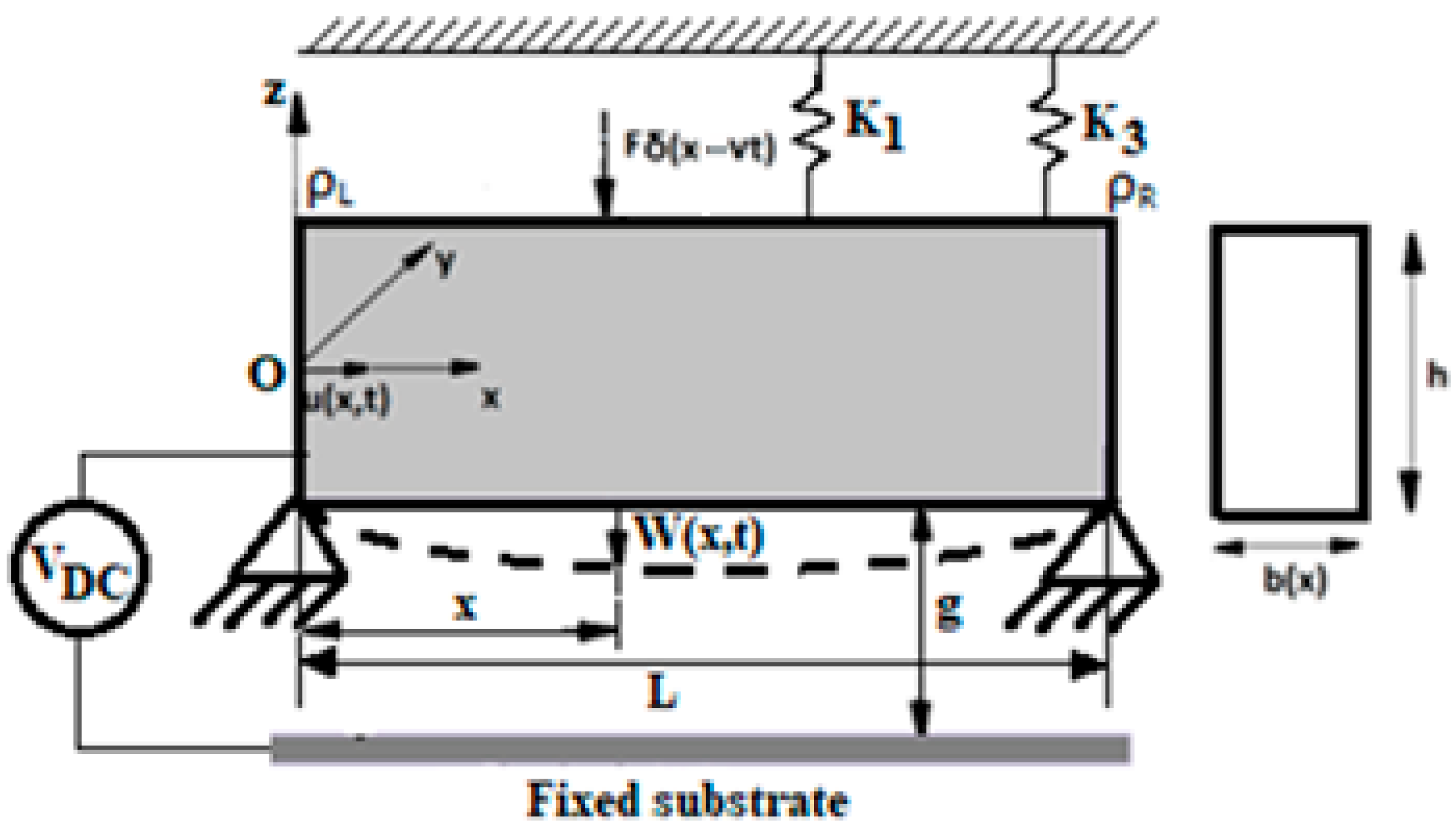
The model of an FGB resting on a nonlinear foundation is shown in Figure 1.

The beam has length L, height h, and width b, which varies along the length of the beam. The beam is subjected to a moving load with constant force F, electromagnetic actuation with bias voltage V_DC, and Casimir force. The system of coordinates has x-, y-, and z- axes, representing the length, width, and height directions, respectively.

The material properties of an Euler–Bernoulli axially FGB, such as its Young’s modulus E, Poisson’s ratio ν, shear modulus μ, and density ρ, and its geometric properties, such as its cross-sectional area A and second moment of inertia I, vary continuously throughout the length of the beam, according to a power law as follows:

$$\begin{array}{l}E(x)=E_R+{\left(1-{\displaystyle \frac{x}{L}}\right)}^n\left(E_L-E_R\right),\mathsf{\nu }(x)={\mathsf{\nu }}_R+{\left(1-{\displaystyle \frac{x}{L}}\right)}^n\left({\mathsf{\nu }}_L-{\mathsf{\nu }}_R\right),b(x)=b_{R+}{\left(1-{\displaystyle \frac{x}{L}}\right)}^n\left(b_L-b_R\right)\\ \mathsf{\mu }(x)={\displaystyle \frac{E(x)}{2[1+\mathsf{\nu }(x)]}},\mathsf{\rho }(x)={\mathsf{\rho }}_R+{\left(1-{\displaystyle \frac{x}{L}}\right)}^n\left({\mathsf{\rho }}_L-{\mathsf{\rho }}_R\right),h_R=h_L=h,A(x)={\displaystyle {\int }_{A}dA},I(x)={\displaystyle {\int }_A{z}^{2}dA}\end{array}$$

(1)

where n is the volume fraction and exponent and subscripts L and R denote the “left” and “right” ends of the FGB.

According to the Euler–Bernoulli beam theory, the components of the displacement field along the x-, y-, and z-directions can be expressed as follows [6,10,17,18]:

$$u_x(x,z,t)=u(x,t)-z{\displaystyle \frac{\partial W(x,t)}{\partial x}},u_y(x,z,t)=0,u_z(x,z,t)=W(x,t)$$

(2)

where u(x,t) and W(x,t) are the displacement components in the mid-plane along the x- and z-directions, respectively, and $\partial W/\partial x$ is the rotation angle about the y-axis.

The von Kármán-type nonlinear strain displacement relationship gives

$${\mathsf{\epsilon }}_{xx}={\displaystyle \frac{\partial u}{\partial x}}+{\displaystyle \frac{1}{2}}{\left({\displaystyle \frac{\partial W}{\partial x}}\right)}^2-z{\displaystyle \frac{{\partial }^{2}W}{\partial x^2}}$$

(3)

The elastic potential energy of a shear-deformable FGB is

$$U={\displaystyle \frac{1}{2}}{\displaystyle {\int }_0^L\left\{E(x)A(x){\left[\frac{\partial u}{\partial x}+\frac{1}{2}{\left(\frac{\partial W}{\partial x}\right)}^2\right]}^2+E(x)I(x)\left({\frac{{\partial }^{2}W}{\partial x^2}/\sqrt{1+{\left(\frac{\partial W}{\partial x}\right)}^2}}^3\right)\right\}}dx$$

(4)

The kinetic energy of a FGB shear-deformable beam can be written as

$$\mathcal{T}={\displaystyle \frac{1}{2}}{\int }_0^L\rho \left(x\right)\left[A(x){\left({\displaystyle \frac{\partial u}{\partial t}}\right)}^2+I(x){\left({\displaystyle \frac{{\partial }^{2}W}{\partial x\partial t}}\right)}^2+A(x){\left({\displaystyle \frac{\partial W}{\partial t}}\right)}^2\right]dx$$

(5)

The external work done by the impact force F, the electromagnetic actuator, Casimir force, and Winkler–Pasternak foundation is

$$V={\displaystyle {\int }_0^L\left[F\mathsf{\delta }(x-vt)W(x,t)+\frac{C_0{V}_{DC}^2}{2}\left(\frac{1}{g+W}-\frac{1}{g-W}\right)+\frac{{\mathsf{\pi }}^2\hslash cb}{720{(g-W)}^4}+\frac{1}{2}{k}_1{W}^2+\frac{1}{4}{k}_3{W}^4\right]}dx$$

(6)

where δ(x − vt) is the Dirac delta function, C₀ is the capacitance of the actuator, V_DC is the voltage, g is the gap width, $\hslash$ is the reduced Plank’s constant $\hslash =1.055·{10}^{-34}\mathrm{J}\mathrm{s}$, c is the speed of light, $c=2.998·{10}^8\mathrm{m}{\mathrm{s}}^{-1}$, and k₁ and k₃ are linear and nonlinear coefficients, respectively, on the Winkler–Pasternak foundation.

By substituting Equations (4)–(6) into the Hamiltonian principle

$$\delta {\int }_{t_1}^{t_2}[\mathcal{T}-(U+V\left)\right]dt=0$$

(7)

and then performing some simple mathematical manipulations, integrating by parts, and setting the coefficients of δU and δW to zero, one can obtain the following partial differential equations:

$$\mathsf{\rho }(x)A(x){\displaystyle \frac{{\partial }^{2}u}{\partial t^2}}-{\displaystyle \frac{\partial }{\partial x}}\left\{E(x)A(x)\left[{\displaystyle \frac{\partial u}{\partial x}}+{\displaystyle \frac{1}{2}}{\left({\displaystyle \frac{\partial W}{\partial x}}\right)}^2\right]\right\}=0$$

(8)

$$\begin{array}{l}\mathsf{\rho }(x)A(x){\displaystyle \frac{{\partial }^{2}W}{\partial t^2}}-{\displaystyle \frac{\partial }{\partial x}}\left\{E(x)A(x)\left[{\displaystyle \frac{\partial u}{\partial x}}+{\displaystyle \frac{1}{2}}{\left({\displaystyle \frac{\partial W}{\partial x}}\right)}^2\right]\right\}-{\displaystyle \frac{{\partial }^2}{\partial x^2}}\left[E(x)I(x)\left.{{\displaystyle \frac{{\partial }^{2}W}{\partial x^2}}/\sqrt{1+{\left({\displaystyle \frac{\partial W}{\partial x}}\right)}^2}}^3\right]\right.-\\ -F\mathsf{\delta }(x-vt)-{\displaystyle \frac{C_0{V}_{DC}^2}{2}}\left({\displaystyle \frac{1}{{\left(g-W\right)}^2}}-{\displaystyle \frac{1}{{\left(g+W\right)}^2}}\right)-{\displaystyle \frac{{\mathsf{\pi }}^2\hslash cb}{240{(g-W)}^4}}-k_{1}W-k_3{W}^3=0\end{array}$$

(9)

The clamped–clamped boundary conditions at both ends imply that

$$u(0,t)=u(L,t)=0,\hspace{1em}W(0,t)=W(L,t)=0,\hspace{1em}{\displaystyle \frac{\partial W(0,t)}{\partial x}}={\displaystyle \frac{\partial W(L,t)}{\partial x}}=0$$

(10)

According to the governing Equation (9), the term that defines the curvature of the beam can be written in the form:

$${{\displaystyle \frac{{\partial }^{2}W}{\partial x^2}}/\sqrt{1+{\left({\displaystyle \frac{\partial W}{\partial x}}\right)}^2}}^3\approx {\displaystyle \frac{{\partial }^{2}W}{\partial x^2}}\left[1-{\displaystyle \frac{3}{2}}{\left({\displaystyle \frac{\partial W}{\partial x}}\right)}^2\right]$$

(11)

The expression of electromagnetic actuation from Equation (9) can be simplified to the form

$${\displaystyle \frac{C_0{V}_{DC}^2}{2}}\left({\displaystyle \frac{1}{{\left(g-W\right)}^2}}-{\displaystyle \frac{1}{{\left(g+W\right)}^2}}\right)={\displaystyle \frac{C_0{V}_{DC}^2}{2g^2}}\left({\displaystyle \frac{1}{{\left(1-\frac{W}{g}\right)}^2}}-{\displaystyle \frac{1}{{\left(1+\frac{W}{g}\right)}^2}}\right)\approx {\displaystyle \frac{2C_0{V}_{DC}^2}{g^2}}\left[{\displaystyle \frac{W}{g}}+2{\left({\displaystyle \frac{W}{g}}\right)}^3+3.0925{\left({\displaystyle \frac{W}{g}}\right)}^5\right]$$

(12)

The expression of Casimir force can be approximated as

$${\displaystyle \frac{{\mathsf{\pi }}^2\hslash cb}{240{(g-W)}^4}}={\displaystyle \frac{{\mathsf{\pi }}^2\hslash cb}{240g^4}}{\displaystyle \frac{1}{{\left(1-\frac{W}{g}\right)}^4}}\approx {\displaystyle \frac{{\mathsf{\pi }}^2\hslash cb}{240g^4}}\left[1+4{\displaystyle \frac{W}{g}}+10{\left({\displaystyle \frac{W}{g}}\right)}^2+20{\left({\displaystyle \frac{W}{g}}\right)}^3+35{\left({\displaystyle \frac{W}{g}}\right)}^4+56{\left({\displaystyle \frac{W}{g}}\right)}^5\right]$$

(13)

It is remarkable that the maximum errors between the functions appearing in Equations (11)–(13), expressed as

$$\begin{gathered} F_1\left(W\right)={\displaystyle \frac{1}{{\sqrt{1+{\left(\frac{\partial W}{\partial x}\right)}^2}}^3}};F_2(W)=1-{\displaystyle \frac{3}{2}}{\left({\displaystyle \frac{\partial W}{\partial x}}\right)}^2 \\ {F}_3({\displaystyle \frac{W}{g}})={\displaystyle \frac{1}{{\left(1-\frac{W}{g}\right)}^2}}-{\displaystyle \frac{1}{{\left(1+\frac{W}{g}\right)}^2}};F_4({\displaystyle \frac{W}{g}})={\displaystyle \frac{W}{g}}+2{\left({\displaystyle \frac{W}{g}}\right)}^3+3.0925{\left({\displaystyle \frac{W}{g}}\right)}^5 \\ {F}_5({\displaystyle \frac{W}{g}})={\displaystyle \frac{1}{{\left(1-\frac{W}{g}\right)}^4}}; \\ {F}_6({\displaystyle \frac{W}{g}})=1+4{\displaystyle \frac{W}{g}}+10{\left({\displaystyle \frac{W}{g}}\right)}^2+20{\left({\displaystyle \frac{W}{g}}\right)}^3+35{\left({\displaystyle \frac{W}{g}}\right)}^4+56{\left({\displaystyle \frac{W}{g}}\right)}^5 \end{gathered}$$

(14)

are, respectively,

$$\begin{gathered} {\mathsf{\epsilon }}_1=\underset{{\displaystyle \frac{\partial W}{\partial x}}\in [0,0.15]}{\max }\left|F_1\left(W\right)-F_1\left(W\right)\right|=8.4\cdot {10}^{-5} \\ {\mathsf{\epsilon }}_2=\underset{{\displaystyle \frac{W}{g}}\in [0,0.15]}{\max }\left|F_3\left({\displaystyle \frac{W}{g}}\right)-F_4\left({\displaystyle \frac{W}{g}}\right)\right|=3.3\cdot {10}^{-6} \\ {\mathsf{\epsilon }}_3=\underset{{\displaystyle \frac{W}{g}}\in [0,0.15]}{\max }\left|F_5\left({\displaystyle \frac{W}{g}}\right)-F_6\left({\displaystyle \frac{W}{g}}\right)\right|=4.7\cdot {10}^{-6} \end{gathered}$$

(15)

Concerning the Casimir force, for an easier further handling of analytical developments, an adequate truncation is proposed, which simplifies further developments in the condition of inducing an absolute negligible ε₃ error, ensuring an excellent approximation with huge benefits for ulterior computations.

Inserting Equations (11)–(13) into Equation (9) yields

$$\begin{array}{l}\mathsf{\rho }(x)A(x){\displaystyle \frac{{\partial }^{2}W}{\partial t^2}}-{\displaystyle \frac{\partial }{\partial x}}\left\{E(x)A(x)\left[{\displaystyle \frac{\partial u}{\partial x}}+{\displaystyle \frac{1}{2}}{\left({\displaystyle \frac{\partial W}{\partial x}}\right)}^2\right]\right\}-{\displaystyle \frac{{\partial }^2}{\partial x^2}}\left[E(x)I(x)\left.{\displaystyle \frac{{\partial }^{2}W}{\partial x^2}}\left(1-{\displaystyle \frac{3}{2}}{\left({\displaystyle \frac{\partial W}{\partial x}}\right)}^2\right)\right]\right.-k_{1}W-k_3{W}^3-\\ -{\displaystyle \frac{2C_0{V}_{DC}^2}{g^2}}\left[{\displaystyle \frac{W}{g}}+2{\left({\displaystyle \frac{W}{g}}\right)}^3+3.0925{\left({\displaystyle \frac{W}{g}}\right)}^5\right]-{\displaystyle \frac{{\mathsf{\pi }}^2\hslash cb}{240g^4}}\left[1+4{\displaystyle \frac{W}{g}}+10{\left({\displaystyle \frac{W}{g}}\right)}^2+20{\left({\displaystyle \frac{W}{g}}\right)}^3+35{\left({\displaystyle \frac{W}{g}}\right)}^4+56{\left({\displaystyle \frac{W}{g}}\right)}^5\right]=F\mathsf{\delta }(x-vt)\end{array}$$

(16)

The following nondimensional quantities are introduced:

$$\begin{array}{l}\overline{W}={\displaystyle \frac{W}{d}},\hspace{1em}\overline{x}={\displaystyle \frac{x}{L}},\hspace{1em}\overline{E}={\displaystyle \frac{E(x)}{E_R}},\hspace{1em}\overline{\mathsf{\rho }}={\displaystyle \frac{\mathsf{\rho }(x)}{{\mathsf{\rho }}_R}},\hspace{1em}\overline{A}={\displaystyle \frac{A(x)}{A_0}},\hspace{1em}\overline{I}={\displaystyle \frac{I(x)}{I_R}},\hspace{1em}\overline{t}={\displaystyle \frac{t}{L^2}}\sqrt{{\displaystyle \frac{E_R{I}_R}{{\mathsf{\rho }}_R{A}_R}}},\hspace{1em}\overline{\mathsf{\alpha }}={\displaystyle \frac{2C_0{V}_{DC}^2{L}^4}{E_R{g}^3{I}_R}}\\ \overline{v}=vL\sqrt{{\displaystyle \frac{{\mathsf{\rho }}_R{A}_R}{E_R{I}_R}}},\hspace{1em}\overline{f}={\displaystyle \frac{F{L}^4}{E_R{I}_{R}g}},\hspace{1em}{\overline{\mathsf{\gamma }}}_1={\displaystyle \frac{A_R{L}^2}{I_R}},\hspace{1em}{\overline{\mathsf{\gamma }}}_2={\displaystyle \frac{{\mathsf{\pi }}^2\hslash cb{L}^3}{240g^4{E}_R{I}_R}},\hspace{1em}\mathsf{\lambda }={\displaystyle \frac{g^2}{L^2{I}_R}},\hspace{1em}{\overline{k}}_1={\displaystyle \frac{L^4{k}_1}{E_R{I}_R}},\hspace{1em}{\overline{k}}_3={\displaystyle \frac{g^2{L}^4{k}_3}{E_R{I}_R}}\end{array}$$

(17)

If these parameters are inserted into Equations (8) and (14) and the bars are dropped, for brevity, one can obtain the following nondimensional nonlinear equations:

$$\mathsf{\rho }(x)A(x){\displaystyle \frac{{\partial }^{2}u}{\partial t^2}}-{\displaystyle \frac{d}{dx}}\left\{E(x)A(x)\left[{\mathsf{\gamma }}_1{\displaystyle \frac{\partial u}{\partial x}}+{\displaystyle \frac{1}{2}}{\mathsf{\gamma }}_1\mathsf{\lambda }{\left({\displaystyle \frac{{\partial }^{2}W}{\partial x^2}}\right)}^2\right]\right\}=0$$

(18)

$$\begin{array}{l}\mathsf{\rho }(x)A(x){\displaystyle \frac{{\partial }^{2}W}{\partial t^2}}-{\displaystyle \frac{\partial }{\partial x}}\left\{E(x)A(x)\left[{\mathsf{\gamma }}_1{\displaystyle \frac{\partial u}{\partial x}}+{\displaystyle \frac{1}{2}}{\mathsf{\gamma }}_1\mathsf{\lambda }{\left({\displaystyle \frac{{\partial }^{2}W}{\partial x^2}}\right)}^2\right]{\displaystyle \frac{\partial W}{\partial x}}\right\}-{\displaystyle \frac{{\partial }^2}{\partial x^2}}\left[E(x)I(x)\left.{\displaystyle \frac{{\partial }^{2}W}{\partial x^2}}\left(1-{\displaystyle \frac{3}{2}}{\left({\displaystyle \frac{\partial W}{\partial x}}\right)}^2\right)\right]\right.-\\ -\mathsf{\alpha }\left[W+2W^3+3.0925W^5\right]-{\mathsf{\gamma }}_1\left[1+4W+10W^2+20W^3+35W^4+56W^5\right]-k_{1}W-k_{3}W=f\mathsf{\delta }(x-vt)\end{array}$$

(19)

The boundary conditions (10) for the clamped–clamped FGB are then rewritten as:

$$u(0,t)=u(1,t)=0;\hspace{1em}W(0,t)=W(1,t)=0;\hspace{1em}{\displaystyle \frac{\partial W}{\partial x}}(0,t)={\displaystyle \frac{\partial W}{\partial x}}(1,t)=0$$

(20)

The dimensionless nonlinear partial differential equations in Equations (18) and (19) can be discretized into second-order nonlinear ordinary differential equations using the Galerkin–Bubnov technique:

$$u(x,t)=X(x)\mathsf{\theta }(t),\hspace{1em}W(x,t)=Y(x)T(t)$$

(21)

where X(x) and Y(x) are the eigenfunctions for the clamped–clamped FGB and θ(t) and T(t) are the corresponding generalized coordinates. For the clamped–clamped FGB, the shape functions that satisfy the boundary conditions (20) are chosen in the form

$$X(x)=Y(x)=\sqrt{{\displaystyle \frac{2}{3}}}(1-\cos 2\mathsf{\pi }x)$$

(22)

which satisfies the orthonormality condition

$${\displaystyle {\int }_0^1{X}^2(x)dx={\displaystyle {\int }_0^1{Y}^2(x)dx=1}}$$

(23)

By substituting Equation (21) into (18), multiplying by X(x), and integrating on the domain [0, 1], one can obtain the following nonlinear differential equation for the generalized coordinate θ(t):

$${\displaystyle \frac{d^2\mathsf{\theta }}{d{t}^2}}+{\mathsf{\omega }}_1^2\mathsf{\theta }+a_1{T}^2=0$$

(24)

where

$$\begin{array}{l}{\mathsf{\omega }}_1^2=-{\displaystyle \frac{{\mathsf{\gamma }}_1}{{\displaystyle {\int }_0^1\mathsf{\rho }(x)A(x)X^2(x)dx}}}\left[{\displaystyle {\int }_0^1\left(\frac{dE(x)}{dx}A(x)+E(x)\frac{dA(x)}{dx}\right)\frac{dX(x)}{dx}X(x)}dx+{\displaystyle {\int }_0^{1}E(x)A(x)\left.\frac{d^{2}X(x)}{d{x}^2}X(x)dx\right]}\right.\\ a_1=-{\displaystyle \frac{\mathsf{\lambda }{\mathsf{\gamma }}_1}{{\displaystyle {\int }_0^1\mathsf{\rho }(x)A(x)X^2(x)dx}}}\left[{\displaystyle \frac{1}{2}}{\displaystyle {\int }_0^1\left(\frac{dE(x)}{dx}A(x)+E(x)\frac{dA(x)}{dx}\right)\frac{d^{2}Y(x)}{d{x}^2}X(x)}\right.dx+{\displaystyle {\int }_0^{1}E(x)A(x)\left.\frac{d^{2}Y(x)}{d{x}^2}\frac{d^{3}Y(x)}{d{x}^2}X(x)dx\right]}\end{array}$$

(25)

The initial conditions for the nonlinear equation in Equation (24) are:

$$\mathsf{\theta }(0)=A,\hspace{1em}{\displaystyle \frac{d\mathsf{\theta }}{dt}}=0$$

(26)

Now, by substituting Equation (21) into (19), multiplying with Y(x), and integrating on the domain [0, 1], one can obtain

$${\displaystyle \frac{d^{2}T}{d{t}^2}}-a_2\mathsf{\theta }T+{\mathsf{\omega }}_2^{2}T+b_2{T}^2+b_3{T}^3+b_4{T}^4+b_5{T}^5=b_0+f_0\cos 2\mathsf{\pi }vt$$

(27)

where

$$\begin{gathered} \begin{array}{l}{a}_2={\displaystyle \frac{{\mathsf{\lambda }}_1}{{\displaystyle {\int }_0^1\mathsf{\rho }(x)A(x)Y^2(x)dx}}}{\displaystyle {\int }_0^1\left[\frac{dE(x)}{dx}A(x)\frac{dX(x)}{dx}\frac{dY(x)}{dx}Y(x)\right.+E(x)\frac{dA(x)}{dx}\frac{dX(x)}{dx}\frac{dY(x)}{dx}Y(x)}+\\ +E(x)A(x){\displaystyle \frac{d^{2}X(x)}{d{x}^2}}{\displaystyle \frac{dY(x)}{dx}}Y(x)+E(x)A(x){\displaystyle \frac{dX(x)}{dx}}\left.{\displaystyle \frac{d^{2}Y(x)}{d{x}^2}}Y(x)\right]dx\end{array} \\ \begin{array}{l}{\mathsf{\omega }}_2^2=-{\displaystyle \frac{1}{{\displaystyle {\int }_0^1\mathsf{\rho }(x)A(x)Y^2(x)dx}}}\left\{{\displaystyle \frac{1}{2}}\mathsf{\lambda }{\mathsf{\gamma }}_1\left[{\displaystyle {\int }_0^1\left(\frac{dE(x)}{dx}A(x)\right.}\right.\right.{\left({\displaystyle \frac{d^{2}Y(x)}{d{x}^2}}\right)}^2{\displaystyle \frac{dY(x)}{dx}}Y(x)+E(x){\displaystyle \frac{dA(x)}{dx}}{\displaystyle \frac{d^{2}Y(x)}{d{x}^2}}{\displaystyle \frac{dY(x)}{dx}}Y(x)+\\ +2E(x)A(x){\displaystyle \frac{d^{2}Y(x)}{d{x}^2}}{\displaystyle \frac{d^{3}Y(x)}{d{x}^3}}\left.\left.{\displaystyle \frac{dY(x)}{dx}}Y(x)\right)dx\right]+{\displaystyle {\int }_0^1\left(\frac{d^{2}E(x)}{d{x}^2}\right.}I(x){\displaystyle \frac{d^{2}Y(x)}{d{x}^2}}Y(x)+E(x){\displaystyle \frac{d^{2}I(x)}{d{x}^2}}{\displaystyle \frac{d^{2}Y(x)}{d{x}^2}}Y(x)+\\ +E(x)I(x){\displaystyle \frac{d^{4}Y(x)}{d{x}^4}}Y(x)+2{\displaystyle \frac{dE(x)}{dx}}{\displaystyle \frac{dI(x)}{dx}}{\displaystyle \frac{d^{2}Y(x)}{d{x}^2}}Y(x)+2{\displaystyle \frac{dE(x)}{dx}}I(x){\displaystyle \frac{d^{3}Y(x)}{d{x}^3}}Y(x)+\\ +2E(x){\displaystyle \frac{dI(x)}{dx}}\left.{\displaystyle \frac{d^{3}Y(x)}{d{x}^3}}Y(x)+(k_1+4{\mathsf{\gamma }}_2+\mathsf{\alpha }){\displaystyle {\int }_0^1{Y}^2(x)dx}\right]dx\end{array} \\ {b}_2=-10{\mathsf{\gamma }}_2{\displaystyle \frac{{\displaystyle {\int }_0^1{Y}^3}(x)dx}{{\displaystyle {\int }_0^1\mathsf{\rho }(x)A(x)Y^2(x)dx}}} \\ \begin{array}{l}{b}_3={\displaystyle \frac{3{\mathsf{\lambda }}^2/2}{{\displaystyle {\int }_0^1\mathsf{\rho }(x)A(x)Y^2(x)dx}}}{\displaystyle {\int }_0^1{\displaystyle {\int }_0^1\left(\frac{d^{2}E(x)}{d{x}^2}\right.}I(x)\frac{d^{2}Y(x)}{d{x}^2}{\left(\frac{dY(x)}{dx}\right)}^{2}Y(x)}+E(x){\displaystyle \frac{d^{2}I(x)}{d{x}^2}}{\displaystyle \frac{d^{2}Y(x)}{d{x}^2}}{\left({\displaystyle \frac{dY(x)}{dx}}\right)}^{2}Y(x)+\\ +E(x)I(x){\displaystyle \frac{d^{4}Y(x)}{d{x}^4}}{\left({\displaystyle \frac{dY(x)}{dx}}\right)}^{2}Y(x)+6E(x)I(x){\displaystyle \frac{d^{3}Y(x)}{d{x}^3}}{\displaystyle \frac{d^{2}Y(x)}{d{x}^2}}{\displaystyle \frac{dY(x)}{dx}}Y(x)+2E(x)I(x){\left({\displaystyle \frac{d^{2}Y(x)}{d{x}^2}}\right)}^{3}Y(x)+\\ +2{\displaystyle \frac{dE(x)}{dx}}{\displaystyle \frac{dI(x)}{dx}}{\displaystyle \frac{d^{2}Y(x)}{d{x}^2}}{\left({\displaystyle \frac{dY(x)}{dx}}\right)}^{4}Y(x)+2\left(E(x){\displaystyle \frac{dI(x)}{dx}}+E(x){\displaystyle \frac{dE(x)}{dx}}\right)\left({\displaystyle \frac{d^{3}Y(x)}{d{x}^3}}\right.{\left({\displaystyle \frac{dY(x)}{dx}}\right)}^{2}Y(x)+\\ +2\left.\left.{\left({\displaystyle \frac{d^{2}Y(x)}{d{x}^2}}\right)}^2{\displaystyle \frac{dY(x)}{dx}}Y(x)\right)\right]dx-{\displaystyle \frac{\frac{1}{2}{\mathsf{\gamma }}_1\mathsf{\lambda }}{{\displaystyle {\int }_0^1\mathsf{\rho }(x)A(x)Y^2(x)dx}}}\left({\displaystyle {\int }_0^1\frac{dE(x)}{dx}}\right.A(x){\left({\displaystyle \frac{d^{2}Y(x)}{d{x}^2}}\right)}^2{\displaystyle \frac{dY(x)}{dx}}Y(x)+\\ +E(x){\displaystyle \frac{dA(x)}{dx}}{\left({\displaystyle \frac{d^{2}Y(x)}{d{x}^2}}\right)}^2{\displaystyle \frac{dY(x)}{dx}}Y(x)+2E(x)A(x){\displaystyle \frac{d^{3}Y(x)}{d{x}^3}}{\displaystyle \frac{d^{2}Y(x)}{d{x}^2}}{\displaystyle \frac{dY(x)}{dx}}Y(x)+\\ +E(x)A(x)\left.\left.{\left({\displaystyle \frac{d^{2}Y(x)}{d{x}^2}}\right)}^2\right]dx\right)-{\displaystyle \frac{(k_3+20{\mathsf{\gamma }}_2+2\mathsf{\alpha }){\displaystyle {\int }_0^1{Y}^4(x)}dx}{{\displaystyle {\int }_0^1\mathsf{\rho }(x)A(x)Y^2(x)dx}}}\end{array} \\ {b}_4=-{\displaystyle \frac{35{\mathsf{\gamma }}_2{\displaystyle {\int }_0^1{Y}^5(x)dx}}{{\displaystyle {\int }_0^1\mathsf{\rho }(x)A(x)Y^2(x)dx}}};b_5=-{\displaystyle \frac{(3.0925\mathsf{\alpha }+56{\mathsf{\gamma }}_2){\displaystyle {\int }_0^1{Y}^6(x)dx}}{{\displaystyle {\int }_0^1\mathsf{\rho }(x)A(x)Y^2(x)dx}}} \\ {b}_0={\mathsf{\gamma }}_2{\displaystyle \frac{{\displaystyle {\int }_0^{1}Y(x)dx}}{{\displaystyle {\int }_0^1\mathsf{\rho }(x)A(x)Y^2(x)dx}}}+f\sqrt{{\displaystyle \frac{2}{3}}};\hspace{1em}{f}_0=-\sqrt{{\displaystyle \frac{2}{3}}}f \end{gathered}$$

(28)

For the nonlinear equation in Equation (27) the initial conditions are:

$$T(0)=B,\hspace{1em}\dot{T}(0)=0$$

(29)

Equations (24) and (27) with initial conditions (26) and (29), respectively, are second-order nonlinear forced differential equations for which it is very hard to find exact solutions. Therefore, in what follows, for Equations (24), (26), (27) and (29), the OHAM is applied to obtain an approximate analytical solution of high accuracy.

3. The Optimal Homotopy Asymptotic Method

The OHAM is an original procedure proposed by Marinca and Herisanu [33,34,35,36,37]. We consider a general nonlinear differential equation of the form

$$L[Z(t)]+N[Z(t)]=0,\hspace{1em}t\in D$$

(30)

with initial/boundary conditions

$$B\left[Z(t),{\displaystyle \frac{dZ(t)}{dt}}\right]=0$$

(31)

where F is an unknown variable, L and N are linear and nonlinear operators, respectively, t denotes the independent variable, D is the domain of interest, and B is a boundary operator.

If p $\in$ [0, 1] is an embedding parameter, then by means of the OHAM, we can construct a family of equations of the form

$$(1-p)L\left[\overline{Z}(t,p,C_i)\right]=H(t,p,C_i)\left[L(\overline{Z},t,p,C_i)+N(\overline{Z},t,p,C_i)\right]$$

(32)

where $\overline{Z}$ is an unknown approximate solution, C_i, i = 1, 2, …, n are n-many unknown parameters that will be determined later, and H(t, p, C_i) is a non-zero auxiliary function for p $\ne$ 0 and H(t, 0, C_i) = 0. Let us note that the approximate solution $\overline{Z}$ is the sum of only two terms:

$$\overline{Z}(t,p,C_i)=Z_0(t)+p{Z}_1(t,C_1,C_2,\dots ,C_n)$$

(33)

Obviously, when p = 0, it holds that

$$L[Z_0(t)]=0,\hspace{1em}B\left[Z_0(t),{\displaystyle \frac{d{Z}_0(t)}{dt}}\right]=0$$

(34)

from which can be determined the initial approximation Z₀(t). The first approximation Z₁(t, C₁, C₂, …, C_n) can be determined from Equations (32) and (33) for p = 0 and H(t, p, C_i) = pH₀(t, C_i)

$$L[Z_1(t,C_1,C_2,\dots C_n)]=H_0(t,C_i)N[Z_0],\hspace{1em}B\left[Z_1(t),{\displaystyle \frac{d{Z}_1(t)}{dt}}\right]=0$$

(35)

where H₀(t, C_i) is an arbitrary auxiliary function that can be determined, such as the product H₀(t, C_i)N(T₀(t)) and N[T₀(t)] is to be of the same shape (for details see [37]). Without loss of generality, hence in Equation (35), we use only part of the nonlinear term N₀(Z₀).

The parameters C₁, C₂, … C_n, which appear in the first-order approximation Z₁(t, C_i), can be optimally determined in many ways, such as by using the least squares method, the Galerkin method, the collocation method, or the Ritz method, or by minimizing the square residual error:

$$J(C_1,C_2,\dots C_n)={\displaystyle {\int }_0^1{R}^2(t,C_i)}dt$$

(36)

The residual R is given by Equation (30):

$$R(t,C_i)=L\left[\overline{Z}(t)\right]+N\left[\overline{Z}(t)\right]$$

(37)

The unknown parameters C_i can be identified optimally from the conditions:

$${\displaystyle \frac{\partial J}{\partial C_1}}={\displaystyle \frac{\partial J}{\partial C_2}}=\dots ={\displaystyle \frac{\partial J}{\partial C_n}}=0$$

With these convergence-control parameters known, the approximate analytical solution $\overline{Z}$ is well determined. It should be emphasized that the auxiliary function H, the number of convergence-control parameters, and the nonlinear terms N₀(Z₀) are not unique.

4. Application of the OHAM to Nonlinear Forced Vibration of an Axially FGB

In this section, we apply our procedure to obtain an approximate solution to Equations (24), (26), (27), and (29), making the following transformations:

$$\mathsf{\theta }(t)=A\mathsf{\phi }(t),\hspace{1em}T(t)=B\mathsf{\psi }(t),\hspace{1em}\mathsf{\tau }={\mathsf{\Omega }}_{1}t,\hspace{1em}{\mathsf{\tau }}_2={\mathsf{\Omega }}_{2}t$$

(38)

where Ω₁ and Ω₂ are unknown frequencies of the beam corresponding to the displacements u and W, respectively.

The nonlinear differential equations in Equations (24) and (27) can be rewritten as:

$${\mathsf{\phi }}^{″}+{\displaystyle \frac{{\mathsf{\omega }}_1^2}{{\mathsf{\Omega }}_1^2}}\mathsf{\phi }+{\displaystyle \frac{a_1{B}^2}{{\mathsf{\Omega }}_1^{2}A}}{\mathsf{\psi }}^2=0$$

(39)

$${\mathsf{\psi }}^{″}+{\displaystyle \frac{{\mathsf{\omega }}_2^2}{{\mathsf{\Omega }}_2^2}}\mathsf{\psi }-{\displaystyle \frac{a_{2}A}{{\mathsf{\Omega }}_2^2}}\mathsf{\phi }\mathsf{\psi }+{\displaystyle \frac{b_{2}B}{{\mathsf{\Omega }}_2^2}}{\mathsf{\psi }}^2+{\displaystyle \frac{b_3{B}^2}{{\mathsf{\Omega }}_2^2}}{\mathsf{\psi }}^3+{\displaystyle \frac{b_4{B}^3}{{\mathsf{\Omega }}_2^2}}{\mathsf{\psi }}^4+{\displaystyle \frac{b_5{B}^4}{{\mathsf{\Omega }}_2^2}}{\mathsf{\psi }}^5-{\displaystyle \frac{b_0}{B{\mathsf{\Omega }}_2^2}}-{\displaystyle \frac{f_0}{B{\mathsf{\Omega }}_2^2}}\cos {\displaystyle \frac{2\mathsf{\pi }{\mathsf{\tau }}_2}{{\mathsf{\Omega }}_2}}=0$$

(40)

with corresponding initial conditions

$$\mathsf{\phi }(0)=1,\hspace{1em}{\mathsf{\phi }}^{\prime }(0)=0,\hspace{1em}\mathsf{\psi }(0)=1,\hspace{1em}{\mathsf{\psi }}^{\prime }(0)=0$$

(41)

where

$${\mathsf{\phi }}^{\prime }={\displaystyle \frac{d\mathsf{\phi }}{d{\mathsf{\tau }}_1}},\hspace{1em}{\mathsf{\psi }}^{\prime }={\displaystyle \frac{d\mathsf{\psi }}{d{\mathsf{\tau }}_2}}$$

(42)

The linear operators for Equations (39) and (40) are, respectively,

$$L_1(\mathsf{\phi })={\mathsf{\phi }}^{″}+\mathsf{\phi },\hspace{1em}{L}_2(\mathsf{\psi })={\mathsf{\psi }}^{″}+\mathsf{\psi }$$

(43)

The approximate solutions of Equations (39) and (40) are

$$\overline{\mathsf{\phi }}({\mathsf{\tau }}_1)={\mathsf{\phi }}_0({\mathsf{\tau }}_1)+{\mathsf{\phi }}_1({\mathsf{\tau }}_1,C_i),\hspace{1em}\overline{\mathsf{\psi }}({\mathsf{\tau }}_2)={\mathsf{\psi }}_0({\mathsf{\tau }}_2)+{\mathsf{\psi }}_1({\mathsf{\tau }}_2,C_j)$$

(44)

The initial approximation φ₀ and ψ₀ can be determined from Equations (34) and (41):

$${{\mathsf{\phi }}^{″}}_0+{\mathsf{\phi }}_0=0,\hspace{1em}{\mathsf{\phi }}_0(0)=1,\hspace{1em}{{\mathsf{\phi }}^{\prime }}_0(0)=0$$

(45)

$${{\mathsf{\psi }}^{″}}_0+{\mathsf{\psi }}_0=0,\hspace{1em}{\mathsf{\psi }}_0(0)=1,\hspace{1em}{{\mathsf{\psi }}^{\prime }}_0(0)=0$$

(46)

the solutions to which are, respectively,

$${\mathsf{\phi }}_0({\mathsf{\tau }}_1)=\cos {\mathsf{\tau }}_1$$

(47)

$${\mathsf{\psi }}_0({\mathsf{\tau }}_2)=\cos {\mathsf{\tau }}_2$$

(48)

The nonlinear operators corresponding to Equation (39) and (40) are

$$N(\mathsf{\phi })=\left({\displaystyle \frac{{\mathsf{\omega }}_1^2}{{\mathsf{\Omega }}_1^2}}-1\right)\mathsf{\phi }+{\displaystyle \frac{a_1{B}^2}{{\mathsf{\Omega }}_1^{2}A}}$$

(49)

$$N(\mathsf{\psi })=\left({\displaystyle \frac{{\mathsf{\omega }}_2^2}{{\mathsf{\Omega }}_2^2}}-1\right)\mathsf{\psi }-{\displaystyle \frac{a_{2}A}{{\mathsf{\Omega }}_2^2}}\mathsf{\phi }\mathsf{\psi }+{\displaystyle \frac{b_{2}B}{{\mathsf{\Omega }}_2^2}}{\mathsf{\psi }}^2+{\displaystyle \frac{b_3{B}^2}{{\mathsf{\Omega }}_2^2}}{\mathsf{\psi }}^3+{\displaystyle \frac{b_4{B}^3}{{\mathsf{\Omega }}_2^2}}{\mathsf{\psi }}^4+{\displaystyle \frac{b_5{B}^4}{{\mathsf{\Omega }}_2^2}}{\mathsf{\psi }}^5-{\displaystyle \frac{b_0}{B{\mathsf{\Omega }}_2^2}}-{\displaystyle \frac{f_0}{B{\mathsf{\Omega }}_2^2}}\cos {\displaystyle \frac{2\mathsf{\pi }{\mathsf{\tau }}_2}{{\mathsf{\Omega }}_2}}$$

(50)

With the substitution of solution (47) into Equation (49) and solution (48) into Equation (50), it holds that

$$N({\mathsf{\phi }}_0)=\left({\displaystyle \frac{{\mathsf{\omega }}_1^2}{{\mathsf{\Omega }}_1^2}}-1\right)\cos {\mathsf{\phi }}_1+{\displaystyle \frac{a_1{B}^2}{2{\mathsf{\Omega }}_1^{2}A}}(1+\cos 2{\mathsf{\tau }}_1)$$

(51)

$$N({\mathsf{\psi }}_0)=D_0+D_1\cos {\mathsf{\tau }}_2+D_2\cos 2{\mathsf{\tau }}_2+D_3\cos 3{\mathsf{\tau }}_2+D_4\cos 4{\mathsf{\tau }}_2+D_5\cos 5{\mathsf{\tau }}_2-{\displaystyle \frac{b_0}{B{\mathsf{\Omega }}_2^2}}-{\displaystyle \frac{f_0}{B{\mathsf{\Omega }}_2^2}}\cos {\displaystyle \frac{2\mathsf{\pi }{\mathsf{\tau }}_2}{{\mathsf{\Omega }}_2}}$$

(52)

where

$$\begin{array}{l}{D}_0=-{\displaystyle \frac{b_0}{B{\mathsf{\Omega }}_2^2}}+{\displaystyle \frac{b_2{B}^2}{2{\mathsf{\Omega }}_2^2}}+{\displaystyle \frac{3b_3{B}^3}{8{\mathsf{\Omega }}_2^2}},\hspace{1em}{D}_1={\displaystyle \frac{{\mathsf{\omega }}_2^2}{{\mathsf{\Omega }}_2^2}}-1+{\displaystyle \frac{3b_3{B}^2}{4{\mathsf{\Omega }}_2^2}}-{\displaystyle \frac{5b_5{B}^4}{16{\mathsf{\Omega }}_2^2}},\hspace{1em}{D}_2={\displaystyle \frac{b_{2}B}{2{\mathsf{\Omega }}_2^2}}+{\displaystyle \frac{b_4{B}^3}{2{\mathsf{\Omega }}_2^2}}\\ D_3={\displaystyle \frac{b_3{B}^2}{4{\mathsf{\Omega }}_2^2}}+{\displaystyle \frac{5b_5{B}^5}{16{\mathsf{\Omega }}_2^2}},\hspace{1em}{D}_4={\displaystyle \frac{b_4{B}^3}{8{\mathsf{\Omega }}_2^2}},\hspace{1em}{D}_5={\displaystyle \frac{b_5{B}^4}{16{\mathsf{\Omega }}_2^2}}\end{array}$$

(53)

The auxiliary functions for the two equations in Equation (35) corresponding to variables φ₁ and ψ₁ are obtained from Equations (47) and (51) for the variable φ₁ and from Equations (48) and (52) for the variable ψ₁:

$$H_1({\mathsf{\tau }}_1,C_1,C_2,C_3,C_4)=C_1+2C_2\cos {\mathsf{\tau }}_1+2C_3\cos 2{\mathsf{\tau }}_1+2C_{4}vos4{\mathsf{\tau }}_1$$

(54)

$$H_2({\mathsf{\tau }}_2,C_5,C_6,C_7)=C_5+2C_6\cos 2{\mathsf{\tau }}_2+2C_7\cos 3{\mathsf{\tau }}_2$$

(55)

The first approximation φ₁ and ψ₁ are obtained from Equations (25), (54) and (55):

$${{\mathsf{\phi }}^{″}}_1+{\mathsf{\phi }}_1=(C_1+2C_2\cos {\mathsf{\tau }}_1+2C_3\cos 2{\mathsf{\tau }}_1+2C_{4}vos4{\mathsf{\tau }}_1)\left[\left({\displaystyle \frac{{\mathsf{\omega }}_1^2}{{\mathsf{\Omega }}_1^2}}-1\right)\cos {\mathsf{\tau }}_1+{\displaystyle \frac{a_1{B}^2}{2A{\mathsf{\Omega }}_1^2}}\right],\hspace{1em}{\mathsf{\phi }}_1(0)={{\mathsf{\phi }}^{\prime }}_1(0)=0$$

(56)

$${{\mathsf{\psi }}^{″}}_1+{\mathsf{\psi }}_1=(C_5+2C_6\cos 2{\mathsf{\tau }}_2+2C_7\cos 3{\mathsf{\tau }}_2)(D_0+D_1\cos {\mathsf{\tau }}_2+D_3\cos 3{\mathsf{\tau }}_2),\hspace{1em}{\mathsf{\psi }}_1(0)={{\mathsf{\psi }}^{\prime }}_1(0)=0$$

(57)

No secular terms in Equations (56) and (57) requires that the coefficients of cosτ₁ in Equation (56) and cosτ₂ in Equation (57) be zero. From these conditions, one can determine the natural frequencies:

$$\begin{array}{l}{\mathsf{\Omega }}_1^2={\mathsf{\omega }}_1^2+{\displaystyle \frac{a_1{B}^2{C}_2}{A(C_1+C_3)}}\\ {\mathsf{\Omega }}_2^2={\mathsf{\omega }}_2^2+{\displaystyle \frac{3b_3{B}^2}{4}}+{\displaystyle \frac{5b_5{B}^4}{8}}+\left({\displaystyle \frac{b_3{B}^2}{4}}+{\displaystyle \frac{5b_5{B}^4}{16}}\right){\displaystyle \frac{C_6}{C_5+C_6}}\end{array}$$

(58)

After some manipulations, from Equations (56) and (57), it holds that

$$\begin{array}{l}{\mathsf{\phi }}_1({\mathsf{\tau }}_1)=\left[{\displaystyle \frac{a_1{B}^2{C}_1}{2A{\mathsf{\Omega }}_1^2}}+C_2\left({\displaystyle \frac{{\mathsf{\omega }}_1^2}{{\mathsf{\Omega }}_1^2}}-1\right)\right](1-\cos {\mathsf{\tau }}_1)+{\displaystyle \frac{1}{3}}\left[C_2\left({\displaystyle \frac{{\mathsf{\omega }}_1^2}{{\mathsf{\Omega }}_1^2}}-1\right)+{\displaystyle \frac{a_1{B}^2{C}_3}{A{\mathsf{\Omega }}_1^2}}\right](\cos {\mathsf{\tau }}_1-\cos 2{\mathsf{\tau }}_1)+\\ +{\displaystyle \frac{C_3+C_4}{8}}\left({\displaystyle \frac{{\mathsf{\omega }}_1^2}{{\mathsf{\Omega }}_1^2}}-1\right)(\cos {\mathsf{\tau }}_1-\cos 3{\mathsf{\tau }}_1)+{\displaystyle \frac{a_1{B}^2{C}_4}{15A{\mathsf{\Omega }}_1^2}}(\cos {\mathsf{\tau }}_1-\cos 4{\mathsf{\tau }}_1)+{\displaystyle \frac{C_4}{24}}\left({\displaystyle \frac{{\mathsf{\omega }}_1^2}{{\mathsf{\Omega }}_1^2}}-1\right)(\cos {\mathsf{\tau }}_1-\cos 5{\mathsf{\tau }}_1)\end{array}$$

(59)

$$\begin{array}{l}{\mathsf{\psi }}_1({\mathsf{\tau }}_2)=(D_0{C}_5+D_3{C}_7)(1-\cos {\mathsf{\tau }}_2)+{\displaystyle \frac{2D_0{C}_6+D_1{C}_7}{3}}(\cos {\mathsf{\tau }}_2-\cos 2{\mathsf{\tau }}_2)+{\displaystyle \frac{D_1{C}_6+2D_0{C}_7}{8}}(\cos {\mathsf{\tau }}_2-\cos 3{\mathsf{\tau }}_2)+\\ +{\displaystyle \frac{D_1{C}_7}{15}}(\cos {\mathsf{\tau }}_2-\cos 4{\mathsf{\tau }}_2)+{\displaystyle \frac{D_3{C}_7}{35}}(\cos {\mathsf{\tau }}_2-\cos 6{\mathsf{\tau }}_2)\end{array}$$

(60)

The approximate solutions of Equations (24), (26), (27) and (29) are obtained from Equations (38), (44), (47), (48), (59) and (60):

$$\begin{array}{l}\mathsf{\theta }(t)=A\cos {\mathsf{\Omega }}_{1}t+\left[{\displaystyle \frac{a_1{B}^2{C}_1}{2{\mathsf{\Omega }}_1^2}}+A{C}_2\left({\displaystyle \frac{{\mathsf{\omega }}_1^2}{{\mathsf{\Omega }}_1^2}}-1\right)\right](1-\cos {\mathsf{\Omega }}_{1}t)+{\displaystyle \frac{1}{3}}\left[A{C}_2\left({\displaystyle \frac{{\mathsf{\omega }}_1^2}{{\mathsf{\Omega }}_1^2}}-1\right)+{\displaystyle \frac{a_1{B}^2{C}_3}{{\mathsf{\Omega }}_1^2}}\right](\cos {\mathsf{\Omega }}_{1}t-\cos 2{\mathsf{\Omega }}_{1}t)+\\ +{\displaystyle \frac{A(C_3+C_4)}{8}}\left({\displaystyle \frac{{\mathsf{\omega }}_1^2}{{\mathsf{\Omega }}_1^2}}-1\right)(\cos {\mathsf{\Omega }}_{1}t-\cos 3{\mathsf{\Omega }}_{1}t)+{\displaystyle \frac{a_1{B}^2{C}_4}{15{\mathsf{\Omega }}_1^2}}(\cos {\mathsf{\Omega }}_{1}t-\cos 4{\mathsf{\Omega }}_{1}t)+{\displaystyle \frac{A{C}_4}{24}}\left({\displaystyle \frac{{\mathsf{\omega }}_1^2}{{\mathsf{\Omega }}_1^2}}-1\right)(\cos {\mathsf{\Omega }}_{1}t-\cos 5{\mathsf{\Omega }}_{1}t)\end{array}$$

(61)

$$\begin{array}{l}T(t)=B\cos {\mathsf{\Omega }}_{2}t+B(D_0{C}_5+D_3{C}_7)(1-\cos {\mathsf{\Omega }}_{2}t)+{\displaystyle \frac{B(2D_0{C}_6+D_1{C}_7)}{3}}(\cos {\mathsf{\Omega }}_{2}t-\cos 2{\mathsf{\Omega }}_{2}t)+\\ +{\displaystyle \frac{B(D_1{C}_6+2D_0{C}_7)}{8}}(\cos {\mathsf{\Omega }}_{2}t-\cos 3{\mathsf{\Omega }}_{2}t)+{\displaystyle \frac{B{D}_1{C}_7}{15}}(\cos {\mathsf{\Omega }}_{2}t-\cos 4{\mathsf{\Omega }}_{2}t)+{\displaystyle \frac{B{D}_3{C}_7}{35}}(\cos {\mathsf{\Omega }}_{2}t-\cos 6{\mathsf{\Omega }}_{2}t)\end{array}$$

(62)

5. Numerical Examples

To prove the effectiveness of our procedure, we consider the following particular case, for a volume fraction index n = 2, taking into account Equations (25) and (28): A = 0.1, B = 1, v = 0.4, ω₁ = 1.1, ω₂ = 1.5846, a₁ = 0.002, a₂ = 0.055, b₂ = 0.08, b₃ = 0.09, b₄ = 0.012, b₅ = 0.022, b₀ = 0.0011, f₀ = 0.001.

In this case, ${\omega }_2^2\approx 2\pi v$; hence, it follows that this is a case of primary resonance, such that the optimal values of the convergence-control parameters obtained by minimizing the residual error are:

C₁ = −1.47938, C₂ = −1.01765, C₃ = −2.51638, C₄ = 2.79951, C₅ = −0.611716, C₆ = 0.0498806, C₇ = −0.433609

(63)

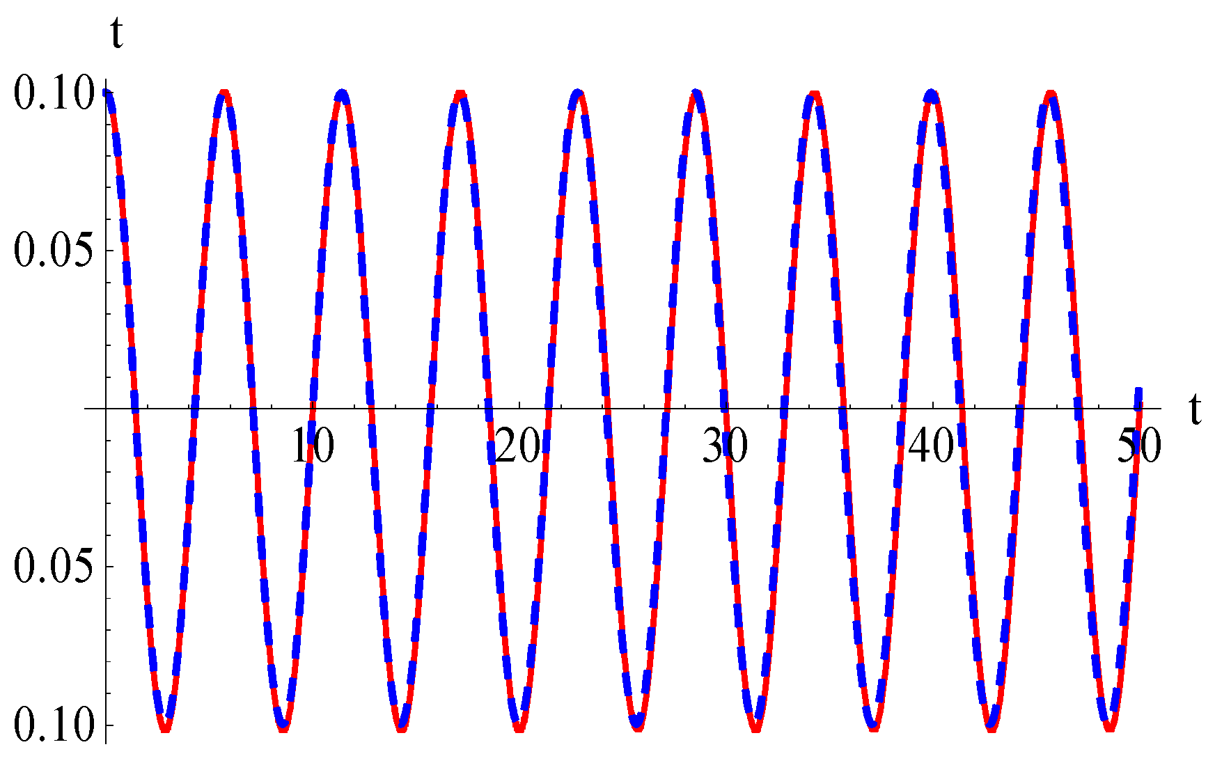
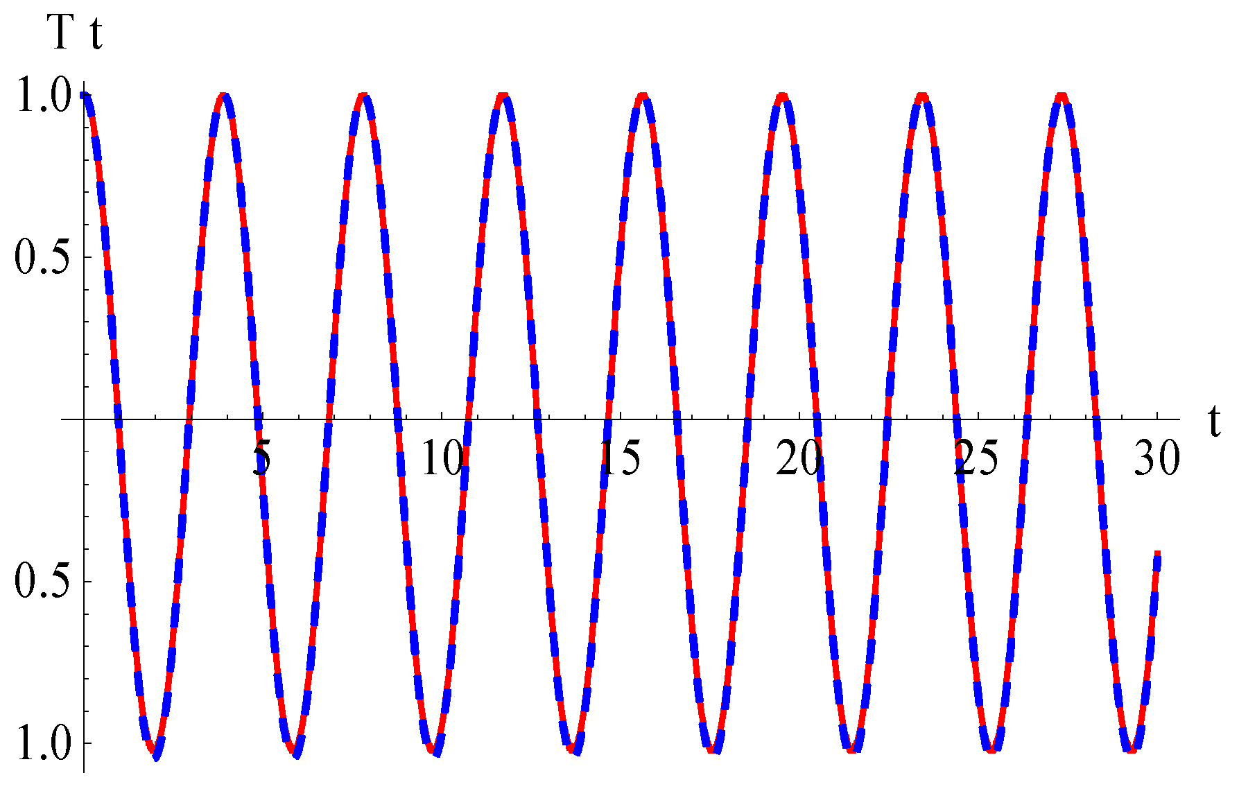
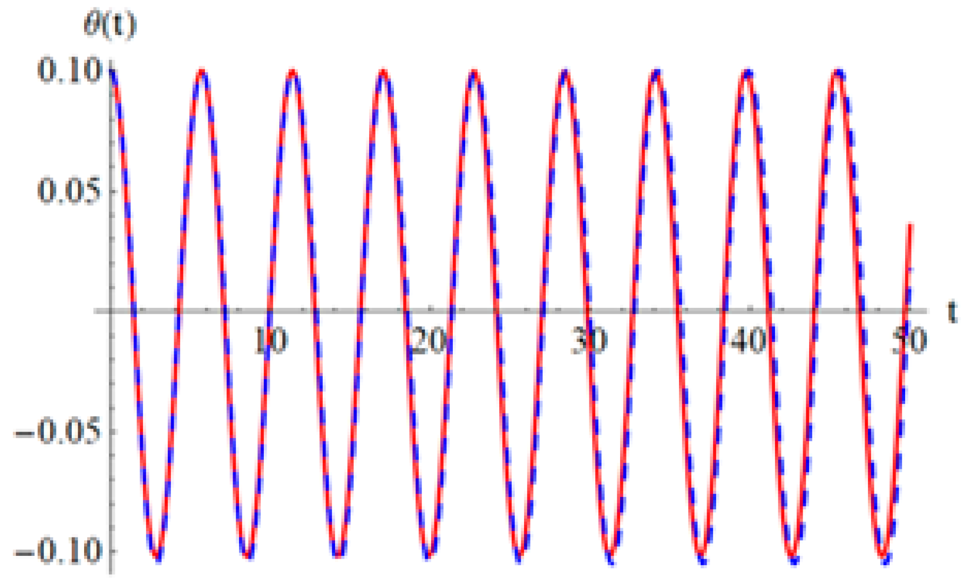
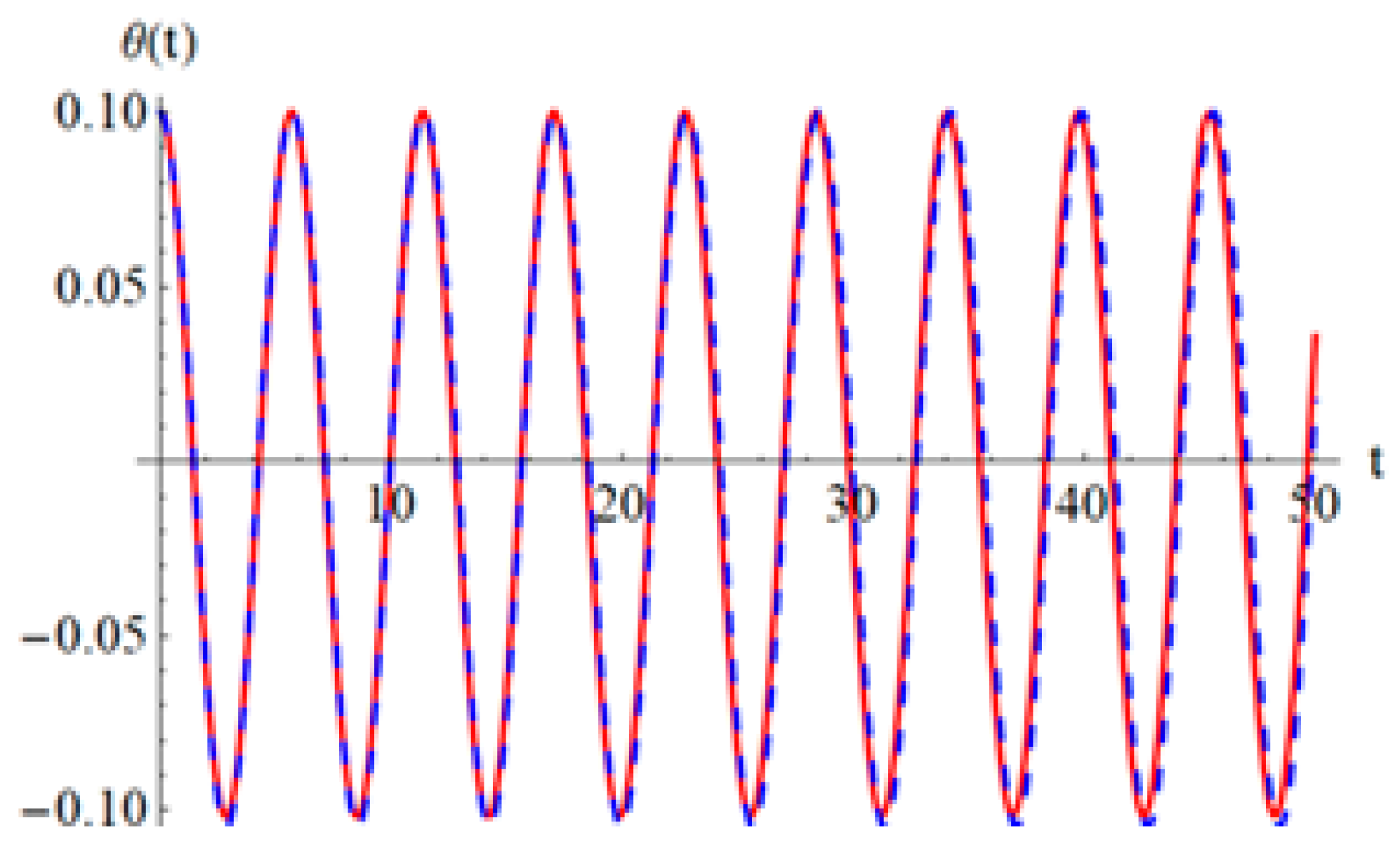
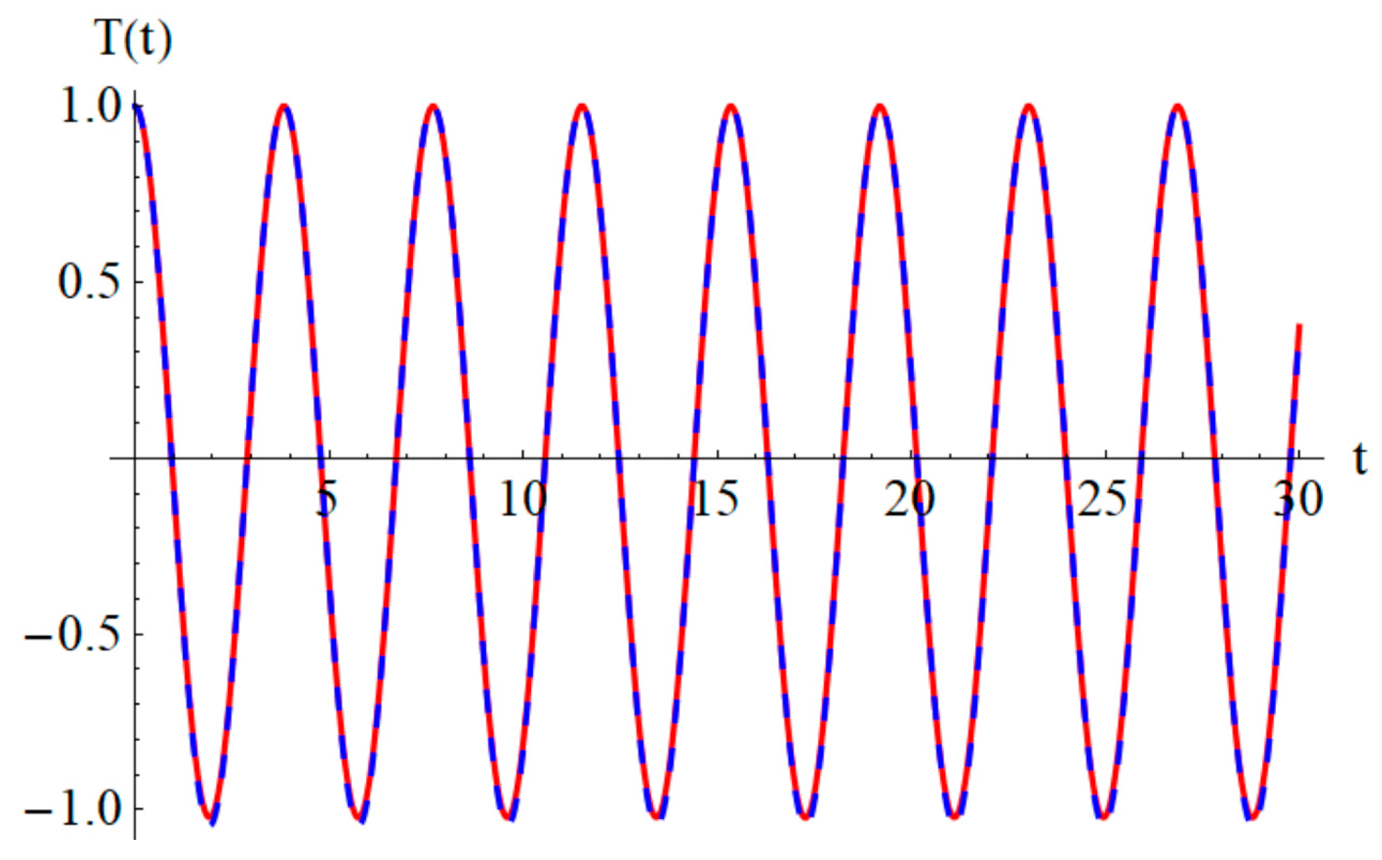
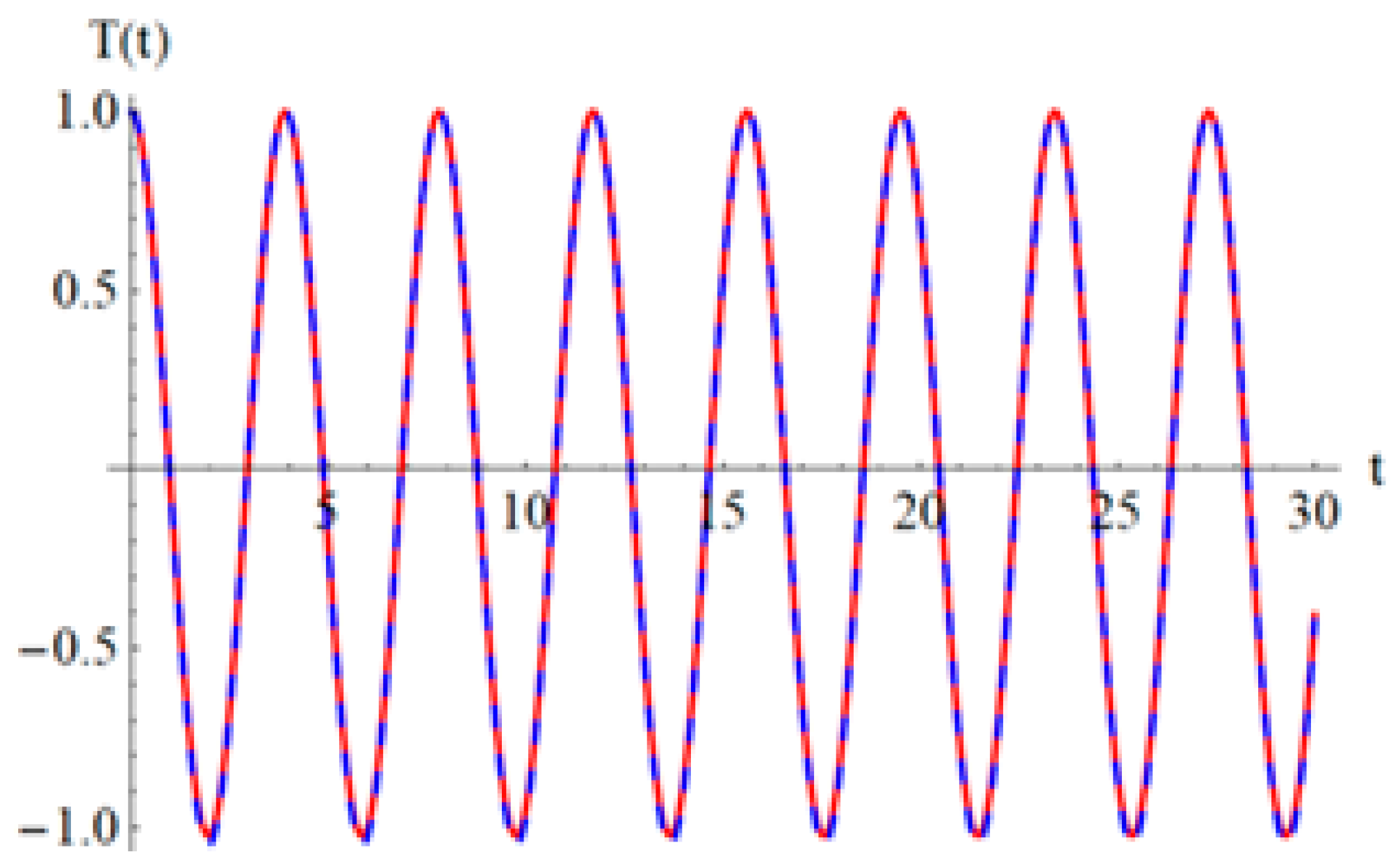
Figure 2 and Figure 3 depict the approximate solution from (61) and the approximate solution from (62), respectively, in comparison with numerical solutions obtained by the classical Fourth-Order Runge–Kutta (RK4) method with a time-step size of 0.05, in the initial conditions (26) and (29).

It can be seen that the errors between the approximate analytical solutions obtained by means of the OHAM and the numerical integration results are very good, the two solutions being in excellent agreement. This comparison validates our technique.

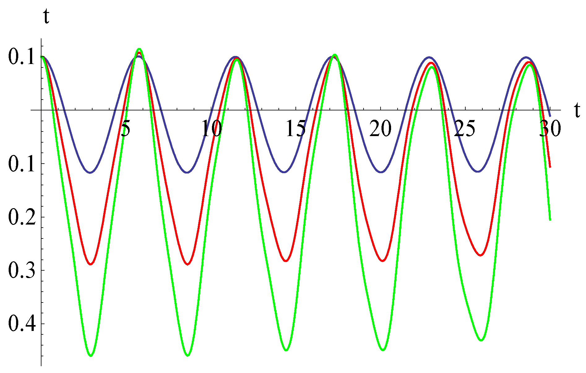
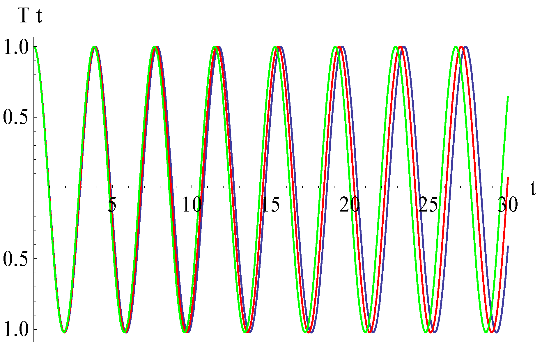
For a different volume fraction index n = 3, it is obtained ω₁ = 1.107, ω₂ = 1.5852, a₁ = 0.00207, a₂ = 0.053, b₂ = 0.081, b₃ = 0.089, b₄ = 0.013, b₅ = 0.022, b₀ = 0.0013 and the optimal values of the convergence-control parameters will be C₁ = −8.15949, C₂ = −8.54795, C₃ = −8.92887, C₄ = −5.26623, C₅ = −0.628662, C₆ = 0.0527305, C₇ = −0.440419, which lead to graphical representations from Figure 4 and Figure 5.

It is clear that a small change in the volume fraction index has a small influence, as can be seen above.

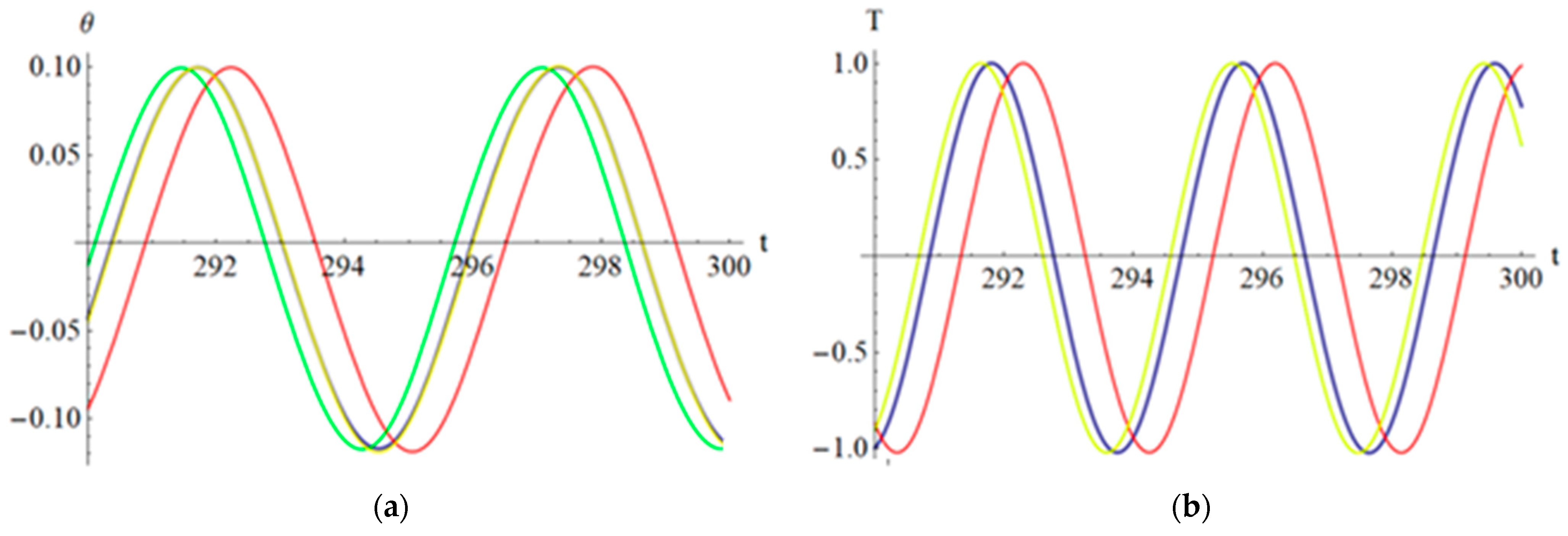
Figure 6 depicts the effect of parameter a₁ on the approximate solution given by (61). It is observed that when a₁ increases, then the period of θ increases, while the maximum amplitude varies slowly up to t = 17. After t = 17, the maximum amplitude decreases. On the other hand, the minimum amplitude decreases on the whole domain.

Figure 7 and Figure 8 present graphs of the variable T(t) for different values of parameters b₃ and b₅, respectively.

One can observe that as the parameter b₃ increases, the period increases very slowly up to t = 8, but for b > 8, the period decreases. As b₅ decreases, then the amplitude varies very slowly, but for t > 8, the amplitude increases.

To study the influence of one of the curvature, Casimir force, electromagnetic actuation, and nonlinear foundation, more precisely, when ${{\displaystyle \frac{{\partial }^{2}W}{\partial x^2}}/\sqrt{1+{\left({\displaystyle \frac{\partial W}{\partial x}}\right)}^2}}^3\approx 0$ (Subcase A); ${\displaystyle \frac{{\pi }^2\hslash cb}{240(g-W{)}^4}}\approx 0$ (Subcase B); ${\displaystyle \frac{C_0{V}_{DC}^2}{2}}\left({\displaystyle \frac{1}{{\left(g-W\right)}^2}}-{\displaystyle \frac{1}{{\left(g+W\right)}^2}}\right)\approx 0$ (Subcase C) and, respectively, ${\displaystyle \frac{1}{2}}{k}_1{W}^2+{\displaystyle \frac{1}{4}}{k}_3{W}^4\approx 0$ (Subcase D), the values of the parameters which appear into Equations (24) and (26) in each of the above defined subcases are computed in

Table 1. The values of the parameters for the considered subcases.

	ω1	ω2	a1	a2	b0	b2	b3	b4	b5	f0
Subcase A	1.12	1.58901	0.021	0.0581	0.0014	0.082	0.091	0.013	0.024	0.001
Subcase B	1.118	1.5873	0.023	0.0587	0.0013	0.079	0.089	0.012	0.021	0.001
Subcase C	1.121	1.5901	0.022	0.0584	0.0014	0.081	0.092	0.014	0.022	0.001
Subcase D	1.12	1.5904	0.023	0.0283	0.0015	0.081	0.09	0.012	0.023	0.001

.

In Figure 9 are presented the effects of the curvature, Casimir force, electromagnetic actuation, and nonlinear foundation, respectively, as described above for the four subcases.

In a particular case related to a strong electromagnetic actuation, the parameters b₃ and b₅ are changed, such as b₃ = 0.11 and b₅ = 0.031, and it follows that ω₂ = 1.6053. In this case, following the same procedure, one obtains the optimal values for the convergence-control parameters: C₁ = 8.13816, C₂ = −8.53364, C₃ = 8.92158, C₄ = −5.26244, C₅ = −0.500756, C₆ = 0.0273566, C₇ = −0.441732. In Figure 10 and Figure 11 are compared the approximate analytical solutions with numerical solutions in this particular case.

6. The Stability of Steady-State Motion in the Case of Primary Resonance

We investigate the local stability of the model by means of the Routh–Hurwitz criterion and the eigenvalues of the Jacobian matrix. Local stability depends on the signs of the eigenvalues, which leads to a study of borderline cases for primary resonance at ${\omega }_2\approx \omega$, $\omega =2\pi v$. With the homotopy perturbation method [38], for p = 0, any nonlinear differential equation reduces to a linear differential equation, and for p = 1, one obtains the original equation. Thus, the original Equations (24) and (27) are rewritten as

$$\ddot{\mathsf{\theta }}+{\mathsf{\omega }}_1^2\mathsf{\theta }+p{a}_1{T}^2=0$$

(64)

$$\ddot{T}+{\mathsf{\omega }}_2^{2}T+p\left[-a_2\mathsf{\theta }T+b_2{T}^2+b_3{T}^3+b_4{T}^4+b_5{T}^5-b_0-f_0\cos \mathsf{\omega }t\right]=0$$

(65)

where p $\in$ [0, 1] is the embedding parameter.

In the case of primary resonance, we have

$$\mathsf{\omega }={\mathsf{\omega }}_2+\mathsf{\Delta }p$$

(66)

with Δ being a detuning parameter.

The procedure applied in this study distinguishes among the three time scales by associating separate independent variables with each one:

$${\mathsf{\xi }}_1={\mathsf{\omega }}_{1}t,\hspace{1em}{\mathsf{\xi }}_2={\mathsf{\omega }}_{2}t,\hspace{1em}\mathsf{\eta }=pt$$

(67)

To substitute Equation (67) into Equations (64) and (65), we need the following expressions:

$$\dot{\mathsf{\theta }}={\displaystyle \frac{\partial \mathsf{\theta }}{\partial \mathsf{\xi }}}{\displaystyle \frac{\partial \mathsf{\xi }}{\partial t}}+{\displaystyle \frac{\partial T}{\partial \mathsf{\eta }}}{\displaystyle \frac{\partial \mathsf{\eta }}{\partial t}}={\mathsf{\omega }}_1{\displaystyle \frac{\partial \mathsf{\theta }}{\partial {\mathsf{\xi }}_1}}+p{\displaystyle \frac{\partial \mathsf{\theta }}{\partial \mathsf{\eta }}}$$

(68)

$$\ddot{\mathsf{\theta }}={\mathsf{\omega }}_1^2{\displaystyle \frac{{\partial }^2\mathsf{\theta }}{\partial {\mathsf{\xi }}_1^2}}+2{\mathsf{\omega }}_{1}p{\displaystyle \frac{{\partial }^2\mathsf{\theta }}{\partial {\mathsf{\xi }}_1\partial \mathsf{\eta }}}+p^2{\displaystyle \frac{{\partial }^2\mathsf{\theta }}{\partial {\mathsf{\eta }}^2}}$$

(69)

$$\dot{T}=\mathsf{\omega }{\displaystyle \frac{\partial T}{\partial {\mathsf{\xi }}_2}}+p{\displaystyle \frac{\partial T}{\partial \mathsf{\eta }}}$$

(70)

$$\ddot{T}={\mathsf{\omega }}^2{\displaystyle \frac{{\partial }^{2}T}{\partial {\mathsf{\xi }}_2^2}}+2\mathsf{\omega }p{\displaystyle \frac{{\partial }^{2}T}{\partial {\mathsf{\xi }}_2\partial \mathsf{\eta }}}+p^2{\displaystyle \frac{{\partial }^{2}T}{\partial {\mathsf{\eta }}^2}}$$

(71)

The variables θ and T can be written as power series of p:

$$\mathsf{\theta }={\mathsf{\theta }}_0+p{\mathsf{\theta }}_1$$

(72)

$$T=T_0+p{T}_1$$

(73)

By substituting Equations (72) and (73) into (64) and (65) and using Equation (66), we have

$${\mathsf{\omega }}_1^2\left({\displaystyle \frac{{\partial }^2{\mathsf{\theta }}_0}{\partial {\mathsf{\xi }}_1^2}}+p{\displaystyle \frac{{\partial }^2{\mathsf{\theta }}_1}{\partial {\mathsf{\xi }}_1^2}}\right)+2{\mathsf{\omega }}_{1}p\left({\displaystyle \frac{{\partial }^2{\mathsf{\theta }}_0}{\partial {\mathsf{\xi }}_1\partial \mathsf{\eta }}}+p{\displaystyle \frac{{\partial }^2{\mathsf{\theta }}_1}{\partial {\mathsf{\xi }}_1\partial \mathsf{\eta }}}\right)+p^2\left({\displaystyle \frac{{\partial }^2{\mathsf{\theta }}_0}{\partial {\mathsf{\eta }}^2}}+p{\displaystyle \frac{{\partial }^2{\mathsf{\theta }}_1}{\partial {\mathsf{\eta }}^2}}\right)+{\mathsf{\omega }}_1^2({\mathsf{\theta }}_0+p{T}_1)+p{a}_1(T_0^2+2p{T}_0{T}_1+p^2{T}_1^2)=0$$

(74)

$$\begin{array}{l}{({\mathsf{\omega }}_2+\mathsf{\Delta }p)}^2\left({\displaystyle \frac{{\partial }^2{T}_0}{\partial {\mathsf{\xi }}_2^2}}+p{\displaystyle \frac{{\partial }^2{T}_1}{\partial {\mathsf{\xi }}_2^2}}\right)+2({\mathsf{\omega }}_2+\mathsf{\Delta }p)p\left({\displaystyle \frac{{\partial }^2{T}_0}{\partial {\mathsf{\xi }}_2\partial \mathsf{\eta }}}+p{\displaystyle \frac{{\partial }^2{T}_1}{\partial {\mathsf{\xi }}_2\partial \mathsf{\eta }}}\right)+p^2\left({\displaystyle \frac{{\partial }^2{T}_0}{\partial {\mathsf{\eta }}^2}}+p{\displaystyle \frac{{\partial }^2{T}_1}{\partial {\mathsf{\eta }}^2}}\right)+\\ +{({\mathsf{\omega }}_2+\mathsf{\Delta }p)}^2(T_0+p{T}_1)+p\left[-a_2({\mathsf{\theta }}_0+p{\mathsf{\theta }}_1)(T_0+p{T}_1)+b_2(T_0^2\right.+2p{T}_0{T}_1+p^2{T}_1^2)+b_3(T_0^3+3p{T}_0^2{T}_1+\\ +3p^2{T}_0{T}_1^2+p^3{T}_1^3)+b_4(T_0^4+4p{T}_0^3{T}_1+6p^2{T}_0^2{T}_1^2+4p^3{T}_0{T}_1^3+p^4{T}_1^4)+b_5(T_0^5+5p{T}_0^4{T}_1+\\ +10p^2{T}_0^3{T}_1^2+10p^3{T}_0^2{T}_1^3+5p^4{T}_0{T}_1^4+p^5\left.T_1^5)-b_0-f_0\cos {\mathsf{\xi }}_2\right]=0\end{array}$$

(75)

From Equations (74) and (75), the homotopy equations of order p⁰ and p¹ are, respectively,

$${\mathrm{P}}^0:{\mathsf{\omega }}_1^2\left({\displaystyle \frac{{\partial }^2{\mathsf{\theta }}_0}{\partial {\mathsf{\xi }}_1^2}}+{\mathsf{\theta }}_0\right)=0$$

(76)

$${\mathsf{\omega }}_2^2\left({\displaystyle \frac{{\partial }^2{T}_0}{\partial {\mathsf{\xi }}_2^2}}+T_0\right)=0$$

(77)

$${\mathrm{P}}^1:{\mathsf{\omega }}_1^2\left({\displaystyle \frac{{\partial }^2{\mathsf{\theta }}_1}{\partial {\mathsf{\xi }}_1^2}}+{\mathsf{\theta }}_1\right)+2{\mathsf{\omega }}_1{\displaystyle \frac{{\partial }^2{\mathsf{\theta }}_0}{\partial {\mathsf{\xi }}_1\partial \mathsf{\eta }}}+a_1{T}_0^2=0$$

(78)

$${\mathsf{\omega }}_2^2\left({\displaystyle \frac{{\partial }^2{T}_1}{\partial {\mathsf{\xi }}_2^2}}+T_1\right)+2{\mathsf{\omega }}_2\mathsf{\Delta }{\displaystyle \frac{{\partial }^2{T}_0}{\partial {\mathsf{\xi }}_2^2}}-a_2{\mathsf{\theta }}_0{T}_0+b_2{T}_0^2+b_3{T}_0^3+b_4{T}_0^4+b_5{T}_0^5-b_0-f_0\cos {\mathsf{\xi }}_2=0$$

(79)

The solutions of linear Equations (76) and (77) with partial derivatives are, respectively,

$${\mathsf{\theta }}_0({\mathsf{\xi }}_1,\mathsf{\eta })=A_1(\mathsf{\eta })\cos {\mathsf{\xi }}_1+A_2(\mathsf{\eta })\sin {\mathsf{\xi }}_1$$

(80)

$$T_0({\mathsf{\xi }}_2,\mathsf{\eta })=A_3(\mathsf{\eta })\cos {\mathsf{\xi }}_2+A_4(\mathsf{\eta })\sin {\mathsf{\xi }}_2$$

(81)

where A₁, A₂, A₃, and A₄ are functions depending on the variable η.

Substituting Equations (89) and (81) into Equations (78) and (79) and avoiding secular terms yields:

$${\displaystyle \frac{d{A}_1}{d\mathsf{\eta }}}=0,\hspace{1em}{\displaystyle \frac{d{A}_2}{d\mathsf{\eta }}}=0$$

(82)

$${\displaystyle \frac{d{A}_3}{d\mathsf{\eta }}}=2\mathsf{\Delta }{A}_4+{\displaystyle \frac{3b_3}{8{\mathsf{\omega }}_2}}(A_4^3+A_3^2{A}_4)+{\displaystyle \frac{5b_5}{16{\mathsf{\omega }}_2}}{(A_3^2+A_4^2)}^2{A}_4$$

(83)

$${\displaystyle \frac{d{A}_4}{d\mathsf{\eta }}}=-2\mathsf{\Delta }{A}_3-{\displaystyle \frac{3b_3}{8{\mathsf{\omega }}_2}}(A_3^3+A_3{A}_4^2)-{\displaystyle \frac{5b_5}{16{\mathsf{\omega }}_2}}{(A_3^2+A_4^2)}^2{A}_3-f_0$$

(84)

The equilibrium points correspond to periodic motion of Equations (82)–(84). To determine them, we set

$${\displaystyle \frac{d{A}_1}{d\mathsf{\eta }}}={\displaystyle \frac{d{A}_2}{d\mathsf{\eta }}}={\displaystyle \frac{d{A}_3}{d\mathsf{\eta }}}={\displaystyle \frac{d{A}_4}{d\mathsf{\eta }}}=0$$

(85)

In this way, the equilibrium points (A_ie i = 1, 2, 3, 4) can be obtained from the following algebraic equations:

$$A_{1e}=\mathit{constant},\hspace{1em}{A}_{2e}=\mathit{constant}$$

(86)

$$A_{4e}\left[2\mathsf{\Delta }+{\displaystyle \frac{3b_3}{8{\mathsf{\omega }}_2}}(A_{3e}^2+A_{4e}^2)+{\displaystyle \frac{5b_5}{16{\mathsf{\omega }}_2}}{(A_{3e}^2+A_{4e}^2)}^2\right]=0$$

(87)

$$A_{3e}\left[2\mathsf{\Delta }+{\displaystyle \frac{3b_3}{8{\mathsf{\omega }}_2}}(A_{3e}^3+A_{4e}^2)+{\displaystyle \frac{5b_5}{16{\mathsf{\omega }}_2}}{(A_{3e}^2+A_{4e}^2)}^2-{\displaystyle \frac{f_0}{A_{3e}}}\right]=0$$

(88)

From Equations (87) and (88), it is possible only the case

$$A_{4e}=0$$

(89)

$${\displaystyle \frac{5b_5}{16{\mathsf{\omega }}_2}}{A}_{3e}^5+{\displaystyle \frac{3b_3}{8{\mathsf{\omega }}_2}}{A}_{3e}^3+2\mathsf{\Delta }{A}_{3e}+f_0=0$$

(90)

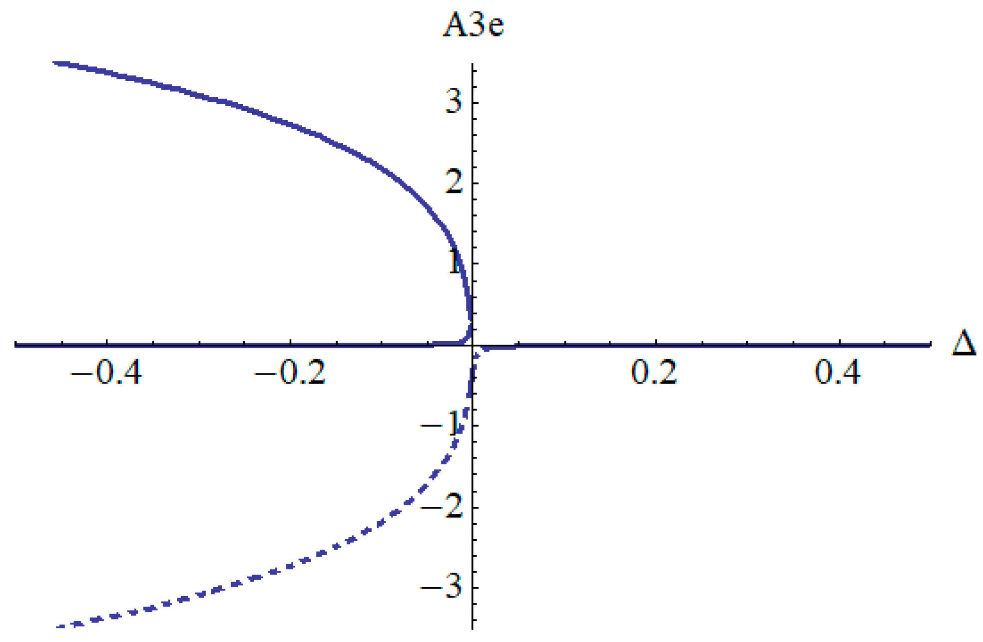
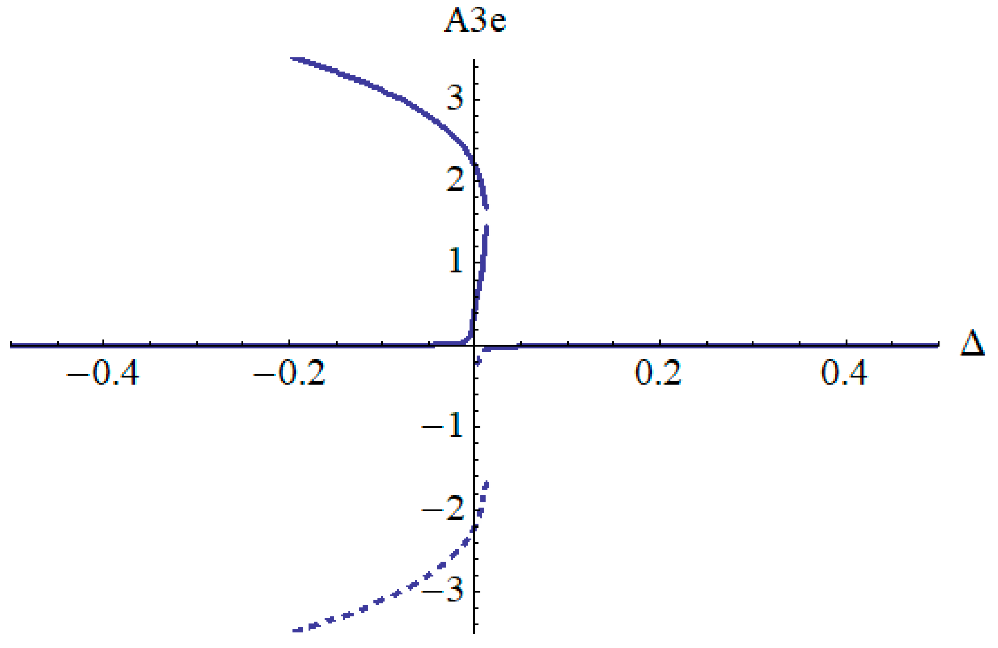
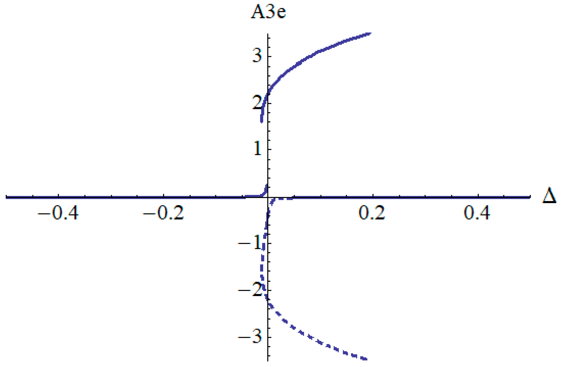
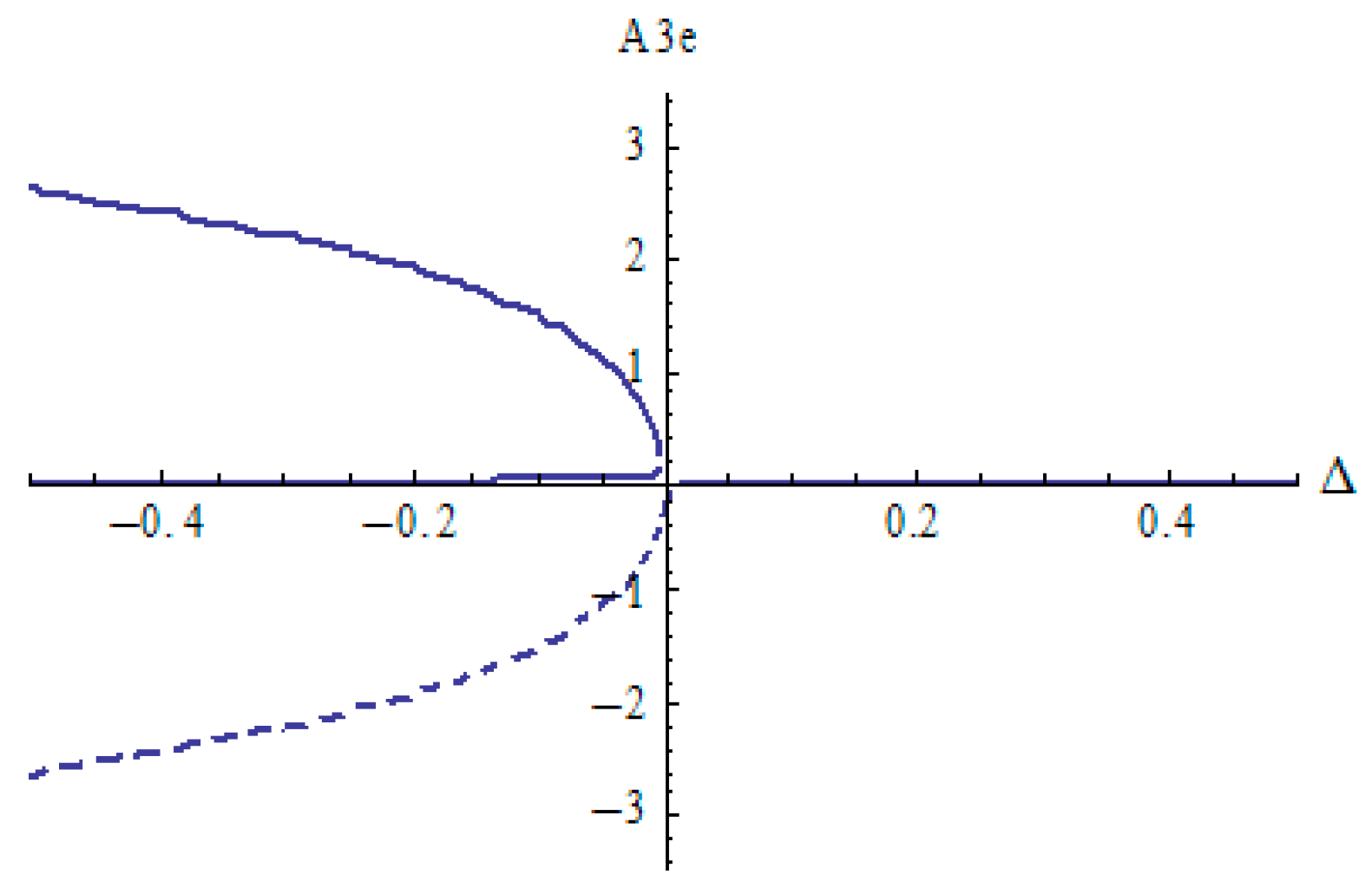
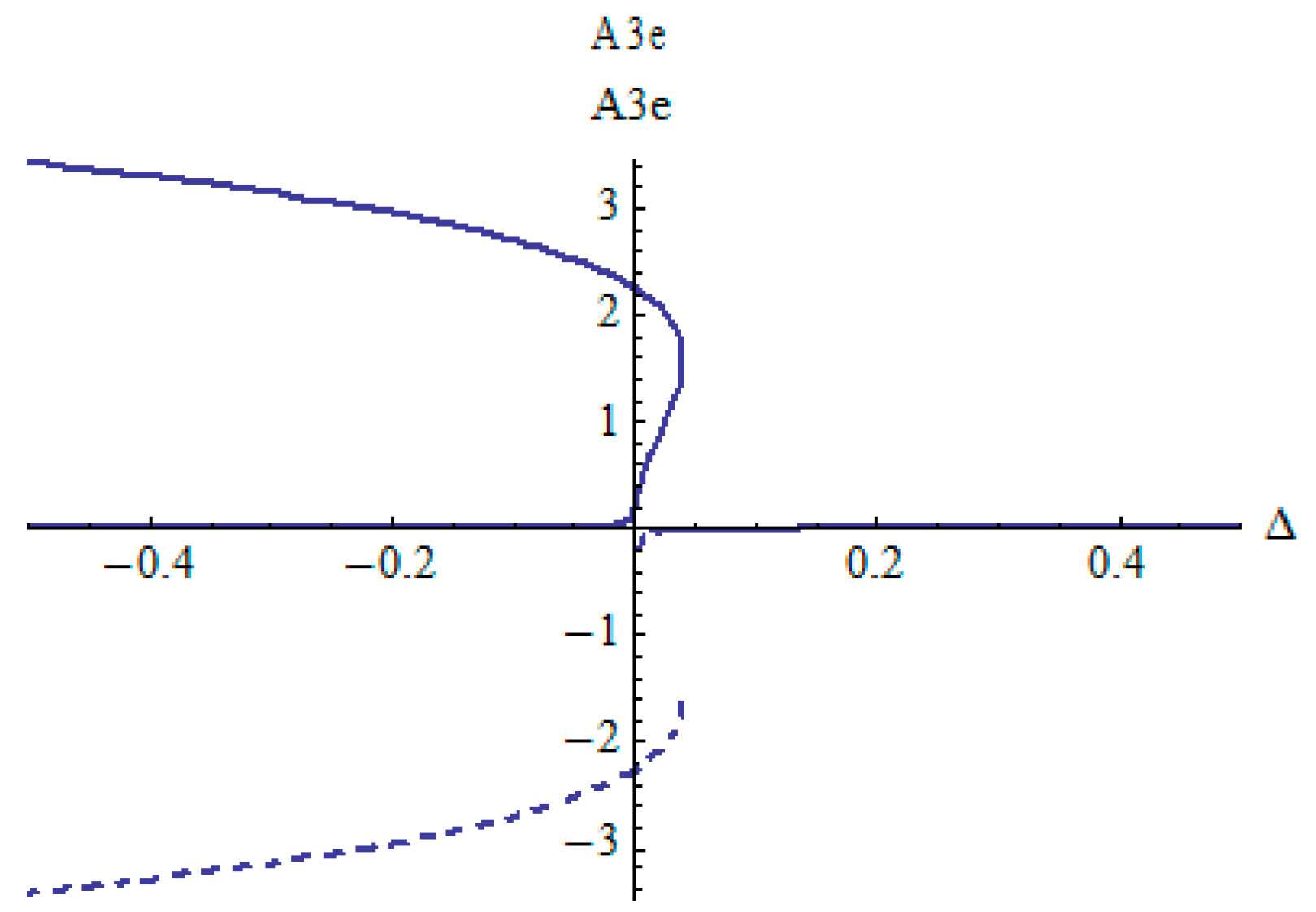
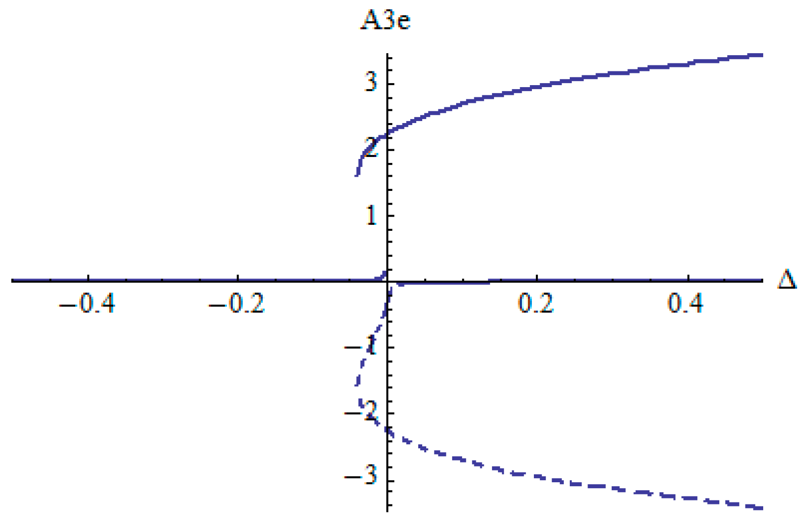
Figure 12, Figure 13 and Figure 14 depict the equilibrium points A_3e with respect to parameter Δ for ω₂ = 1.5846, f₀ = 0.001, and for different values of the parameters b₃ and b₅. For b₃ = 0.09, b₅ = 0.022, Figure 12 shows three existing equilibrium points for Δ ≤ 0 and only one equilibrium point for Δ > 0. For b₃ = −0.09 and b₅ = 0.022 (Figure 13), and for b₃ = 0.09 and b₅ = −0.022 (Figure 14), the situation is the same but with Δ = 0.01 (Figure 13) and Δ ≤ −0.01 (Figure 14).

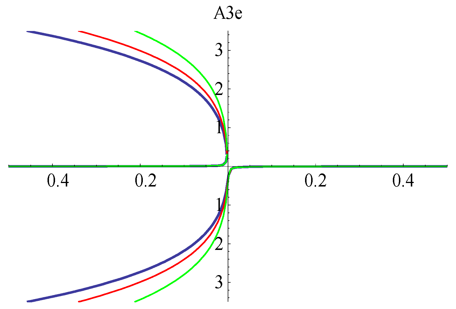
The influence of the parameter ω₂ is shown in Figure 15 for b₃ = 0.09, b₅ = 0.022, and f₀ = 0.001.

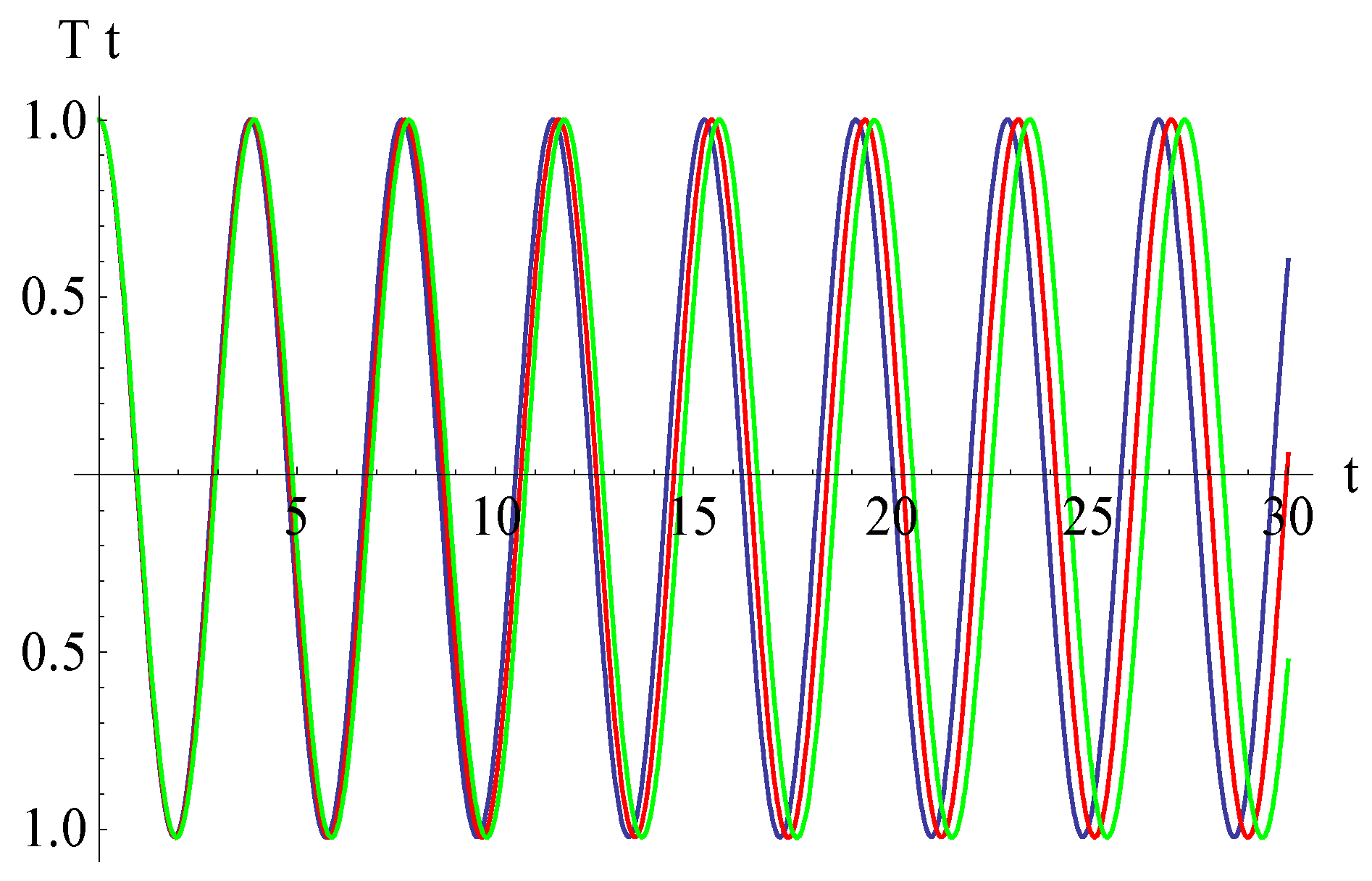
For ω₂ = 1.2846 (blue line), ω₂ = 2.1247 (red line), and ω₂ = 3.4173 (green line), there exist three equilibrium points up to Δ = 0 and only one equilibrium point for Δ > 0.

The stability of the steady-state motion is determined using the eigenvalues of the Jacobian matrix obtained from Equations (82)–(84) (the Routh–Hurwitz criterion)

$$\left[J\right]=\left[a_{ij}\right],\hspace{1em}i,j=1,2,3,4$$

(91)

where

$$a_{1j}={\left.\left({\displaystyle \frac{\partial {A^{\prime }}_1}{\partial A_j}}\right)\right|}_{A_{ie}},\hspace{1em}{a}_{2j}={\left.\left({\displaystyle \frac{\partial {A^{\prime }}_2}{\partial A_j}}\right)\right|}_{A_{ie}},\hspace{1em}{a}_{3j}={\left.\left({\displaystyle \frac{\partial {A^{\prime }}_3}{\partial A_j}}\right)\right|}_{A_{ie}},\hspace{1em}{a}_{4j}={\left.\left({\displaystyle \frac{\partial {A^{\prime }}_4}{\partial A_j}}\right)\right|}_{A_{ie}},\hspace{1em}{A^{\prime }}_i={\displaystyle \frac{\partial A_i}{\partial \mathsf{\eta }}},\hspace{1em}j=1,2,3,4$$

(92)

The non-zero coefficients of the Jacobian matrix are:

$$a_{34}={\displaystyle \frac{5b_5{A}_{3e}^4}{16{\mathsf{\omega }}_2}}+{\displaystyle \frac{3b_3{A}_{3e}^2}{8{\mathsf{\omega }}_2}}+2\mathsf{\Delta }=-{\displaystyle \frac{f_0}{A_{3e}}},\hspace{1em}{a}_{43}=-{\displaystyle \frac{25b_5{A}_{3e}^4}{16{\mathsf{\omega }}_2}}-{\displaystyle \frac{9b_3{A}_{3e}^2}{8{\mathsf{\omega }}_2}}-2\mathsf{\Delta }={\displaystyle \frac{3b_3{A}_{3e}^2}{4{\mathsf{\omega }}_2}}+8\mathsf{\Delta }+{\displaystyle \frac{5f_0}{A_{3e}}}$$

(93)

The eigenvalues of the Jacobian matrix are obtained from the characteristic equation

$$\det \left(\left[J\right]-\mathsf{\lambda }\left[I\right]\right)=0$$

(94)

where I is the unity matrix of the fourth order and λ is the eigenvalue. The characteristic equation in Equation (94) can be rewritten as

$${\mathsf{\lambda }}^2\left[{\mathsf{\lambda }}^2+{\displaystyle \frac{f_0}{A_{3e}}}\left({\displaystyle \frac{3b_3{A}_{3e}^2}{4{\mathsf{\omega }}_2}}+8\mathsf{\Delta }+{\displaystyle \frac{5f_0}{A_{3e}}}\right)\right]=0$$

(95)

where A_3e is obtained from Equation (90). The eigenvalues are:

$${\mathsf{\lambda }}_1={\mathsf{\lambda }}_2=0,\hspace{1em}{\mathsf{\lambda }}_3=-{\mathsf{\lambda }}_4=\sqrt{a},\hspace{1em}a=-{\displaystyle \frac{f_0}{A_{3e}}}\left({\displaystyle \frac{3b_3{A}_{3e}^2}{4{\mathsf{\omega }}_2}}+8\mathsf{\Delta }+{\displaystyle \frac{5f_0}{A_{3e}}}\right)$$

(96)

If a < 0 or ${\displaystyle \frac{3f_0{b}_3{A}_{3e}}{4{\mathsf{\omega }}_2}}+{\displaystyle \frac{8\mathsf{\Delta }{f}_0}{A_{3e}}}+{\displaystyle \frac{5f_0^2}{A_{3e}^2}}>0$, the two eigenvalues are equal to zero and the other two have real parts equal to zero; thus, there is no motion in the directions defined by the corresponding eigenvalues. An important example is the center, when there is a pair of eigenvalues that are purely imaginary, and the signs of their imaginary parts must be opposite. The resulting motion involves points moving around on ellipses, and there is no net motion towards or away from equilibrium.

If a > 0, then there are two zero eigenvalues and two real non-zero eigenvalues (with opposite signs), and points just move parallel to the direction defined by the eigenvector corresponding to the non-zero eigenvalues. This case corresponds to a saddle point. The borderline cases correspond to the case a = 0 or

$$A_{3e}^2+3r{A}_3+2s=0$$

(97)

where

$$r={\displaystyle \frac{32\mathsf{\Delta }{\mathsf{\omega }}_2}{9b_3}},\hspace{1em}s={\displaystyle \frac{10}{3}}{\displaystyle \frac{f_0{\mathsf{\omega }}_2}{b_3}}$$

(98)

If ${\omega }_2<-{\displaystyle \frac{3b_0{b}_3{A}_{3e}^3}{8\mathsf{\Delta }{f}_0{A}_{3e}+5f_0^2}}$, then the equilibrium point A_3e is a center because the eigenvalues are purely imaginary. If ${\omega }_2>-{\displaystyle \frac{3b_0{b}_3{A}_{3e}^3}{8\mathsf{\Delta }{f}_0{A}_{3e}+5f_0^2}}$, then the eigenvalues are real, but in opposite signs and the equilibrium point is a saddle point. 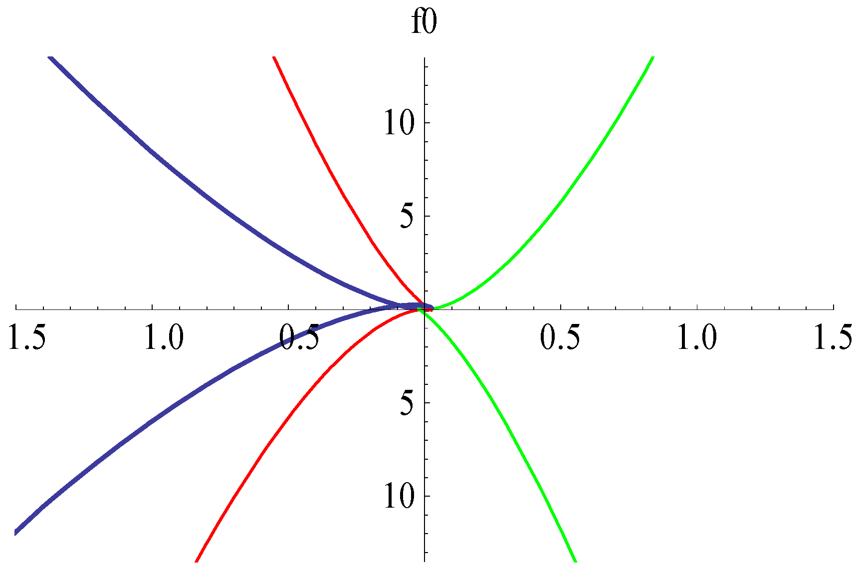If ${\omega }_2=-{\displaystyle \frac{3b_0{b}_3{A}_{3e}^3}{8\mathsf{\Delta }{f}_0{A}_{3e}+5f_0^2}}$, then in Figure 16 is presented the borderline of stability. All three graphs are symmetrical with respect to the horizontal Δ-axis. For example, for ω₂ = 1.5846, b₃ = 0.09, and b₅ = 0.022, the domain between the blue line with Δ = −1.5 and f₀ = 5, correspond to a stable equilibrium point. Also, if Δ = 0.5, and f₀ = 1, the domain of the green line corresponds to a stable equilibrium point.

To study the borderline cases, we consider

$$D=s^2+r^3$$

(99)

and the following distinct cases.

If D > 0, then Equation (97) has a unique real solution:

$${\left(A_{3e}\right)}_1=\sqrt[3]{-s+\sqrt{D}}+\sqrt[3]{-s-\sqrt{D}}$$

(100)

From Equations (90) and (100), we can obtain the condition of existence of the borderline cases.

If D < 0, then Equation (97) has the following real solutions (A_3e) given by Equation (90):

$${\left(A_{3e}\right)}_2={\displaystyle \frac{-1+i\sqrt{3}}{2}}\sqrt[3]{-s+\sqrt{D}}+{\displaystyle \frac{-1-i\sqrt{3}}{2}}\sqrt[3]{-s-\sqrt{D}}$$

(101)

$${\left(A_{3e}\right)}_4={\displaystyle \frac{-1-i\sqrt{3}}{2}}\sqrt[3]{-s+\sqrt{D}}+{\displaystyle \frac{-1+i\sqrt{3}}{2}}\sqrt[3]{-s-\sqrt{D}}$$

(102)

If D = 0, then only the situation −r³ = s² is possible, and

$${\left(A_{3e}\right)}_1=2\sqrt[3]{-s},\hspace{1em}{\left(A_{3e}\right)}_2={\left(A_{3e}\right)}_3=-\sqrt[3]{-s}$$

(103)

From Equations (90) and (97), we can present the borderline cases of stability for our problem with ω₂ = 1.5846 and f₀ = 0.001: for b₃ = 0.09 and b₅ = 0.022 (blue line); for b₃ = −0.09 and b₅ = 0.022 (red line); and for b₃ = 0.09 and b₅ = −0.022 (green line). From these three cases, it is clear that the graph of f₀ is symmetrical with respect to the Δ-axis in all cases.

To study the internal resonance [29], we consider A = 0.1, B = 1, v = 0.4, a₁ = 0.022, a₂ = 0.051, b₂ = 0.08, b₃ = 0.089, b₄ = 0.012, b₅ = 0.021, b₀ = 0.0012, f₀ = 0.001. In this case, we obtain ${\omega }_2\approx {\displaystyle \frac{1}{3}}{\omega }_3$ (internal resonance) and the following graphical results are obtained (Figure 17, Figure 18 and Figure 19).

7. Conclusions

Functionally graded materials, known as nonhomogeneous materials in which the volume fraction varies continuously as a function of spatial position, have been widely used in many fields of engineering, having impact resistance, good designability and manufacturing, and good fatigue, thermal, and acoustical protection properties adequate even for sensors or actuators and energy harvesters. The study of nonlinear motion is essential for devices leading to deformation, noise, cracks, or even failure of structures.

In the present work, we proposed analyzing the nonlinear forced vibration of an axially functionally graded beam based on the von Kármán-type strain–displacement relationship. Considering the curvature of the beam, governing differential equations of motion were established on the basis of moving load, electromagnetic actuation, Casimir force, and a nonlinear elastic foundation. The boundary conditions were considered within the framework of a clamped–clamped Euler–Bernoulli beam. Material properties were expressed according to a power law function through the thickness direction. To truncate the continuous system with an infinite degree of freedom, the Galerkin–Bubnov procedure was applied to reduce the nonlinear partial differential equation of the system to a nonlinear ordinary differential equation. To obtain an approximate analytical solution to the nonlinear dynamical system, the Optimal Homotopy Asymptotic Method was employed. An explicit, highly accurate analytical solution for a complex problem near primary resonance was proposed and applied without requiring additional hypotheses, such as the existence of small parameters into the governing equations or into the boundary/initial conditions. Our technique is based on the existence of some auxiliary functions and a moderate number of convergence-control parameters. These parameters were determined via rigorous mathematical approaches. The effects of the parameters that appear in the nonlinear differential equations were graphically analyzed. The local stability near the primary resonance was determined using the variable expansion method, the homotopy perturbation method, equilibrium points, the Jacobian matrix, and the Routh–Hurwitz criterion. The influence of different parameters on the existence of equilibrium points and borderline cases of stability was studied.