A Hierarchical Reinforcement Learning Approach with Multi-Dimensional State Feature Extraction for Energy-Aware Flexible Job Shop Scheduling

Abstract

Market competition is increasingly intense and sustainable development has attracted widespread attention. The flexible job shop scheduling problem requires the collaborative optimization of production efficiency and machine energy consumption. This scheduling problem has high solution complexity. It is difficult to balance multiple conflicting objectives and obtain stable scheduling results with traditional optimization methods. A Dual-Layer Proximal Policy Optimization algorithm (DL-PPO) based on a hierarchical decision-making mechanism is proposed to achieve the collaborative optimization of production efficiency and energy consumption in solving the Energy-Aware Flexible Job Shop Scheduling Problem (EA-FJSP). First, a hierarchical scheduling framework based on DL-PPO is designed to solve the EA-FJSP. In this framework, the high-level controller selects sub-objectives from a global optimization perspective, while the low-level controller executes feasible dispatching rules according to the selected sub-objectives. Twelve key state features extracted from four dimensions, time, energy consumption, job, and machine, are used to construct a multi-dimensional state space. These features enable a comprehensive state representation of the scheduling environment and provide accurate input for the DL-PPO. The global optimization objective is decomposed into four sub-objectives employing a goal decoupling policy. Four dedicated reward functions are designed for the sub-objectives to guide the low-level controller to make optimal decisions in terms of time and energy consumption, thereby achieving multi-objective collaborative optimization. Considering the two decisions of job selection and machine assignment in solving the EA-FJSP, twenty dual-decision-point dispatching rules are designed as the action space for the low-level controller to achieve the global optimization objective. Finally, the effectiveness, applicability, and superiority of the DL-PPO in EA-FJSP are demonstrated through comparisons with dispatching rules and other deep reinforcement learning methods.

1. Introduction

In the context of green sustainable development, the Energy-Aware Flexible Job Shop Scheduling Problem (EA-FJSP) is an extension of the Flexible Job Shop Scheduling Problem (FJSP) [1,2]. It considers not only traditional efficiency indicators during the scheduling process but is also energy-aware and achieves collaborative optimization. As a typical multi-objective optimization problem, EA-FJSP exhibits higher complexity and has attracted considerable research attention [3]. Similar to studies on traditional multi-objective optimization scheduling problems, the solutions for EA-FJSP include exact [4,5], heuristic [6,7], metaheuristic [8,9,10] and deep reinforcement learning [11,12,13] methods. Exact methods employ mathematical programming to obtain the global optimal solution. As the problem scale enlarges, the computational complexity exhibits exponential growth, rendering them unsuitable for large-scale problem solving [14]. Heuristic methods employ heuristic rules and search strategies to generate high-quality approximate solutions in a shorter period. Characterized by randomness and flexibility, heuristic methods cannot guarantee global optimal solutions owing to the lack of systematic exploration over the solution space [15]. Metaheuristic methods balance solution quality and computational efficiency by intelligently exploring the solution space. However, they require extensive iterative computations when addressing larger-scale problems and are susceptible to local optima [16].

In recent years, Deep Reinforcement Learning (DRL) [17,18] has been widely applied to various job shop scheduling problems due to its strong fitting ability, advantages in solving sequential decision-making problems and characteristics of interaction-based learning. By interacting with the scheduling environment, DRL can learn autonomously and continuously optimize scheduling policies. It addresses the limitations of traditional scheduling methods in utilizing historical scheduling data and provides efficient scheduling solutions for real-world production requirements [19]. Existing studies have shown that DRL exhibits excellent capabilities in scheduling, but it still suffers from low sample efficiency, unstable training, and limited generalization in complex scheduling scenarios. Especially for multi-objective scheduling problems, differences in reward functions and behavioral strategies make it difficult for a single DRL agent to optimize all objectives simultaneously [20]. Nowadays, Hierarchical Reinforcement Learning (HRL) has made significant progress in solving complex decision-making problems [21]. HRL integrates the advantages of hierarchical optimization and DRL. It decomposes complex tasks into easily solvable subtasks and solves them step by step, which enables the derivation of the global policy from the subtask policies. HRL usually uses a two-layer architecture: the high-level controller generates policies and sub-objectives from a global perspective at the macro time scale, while the low-level controller is responsible for achieving these sub-objectives. During the scheduling process, the high-level controller adaptively selects optimization objectives and collaborates with the low-level controller. This enables dynamic balancing among multiple objectives, improving the effectiveness of global optimization. Based on the HRL architecture, this paper proposes a Dual-Layer Proximal Policy Optimization (DL-PPO) algorithm. It simultaneously considers both efficiency and energy consumption objectives in EA-FJSP while reducing the overall solution complexity.

The main contributions are as follows:

• A hierarchical scheduling framework based on DL-PPO is designed for EA-FJSP to minimize the makespan and total energy consumption. In this framework, both the high-level and low-level controllers employ the PPO algorithm to achieve hierarchical and collaborative optimization. The high-level controller determines a temporary optimization objective in accordance with the real-time scheduling state from a global optimization perspective, and the objective is passed to the low-level controller. The low-level controller selects a feasible dispatching rule in accordance with the current state and the temporary optimization objective.
• To reduce the complexity of solving the problem, twelve key state features are extracted from four dimensions: time, energy consumption, job, and machine. These features comprehensively capture the essential characteristics of the scheduling environment while filtering out irrelevant and redundant information, improving the learning efficiency and overall performance of the algorithm.
• In response to the need for collaborative optimization of the makespan and total energy consumption in the EA-FJSP, four sub-objectives are designed for the high-level controller. Each sub-objective is associated with a dedicated reward function to guide the DL-PPO in making optimal decisions in terms of time and energy consumption. Taking into account the two key decisions of job selection and machine assignment in the scheduling process, twenty dual-decision-point dispatching rules are designed as the action space for the low-level controller. This ensures that the low-level controller can select effective scheduling policies to achieve the temporary optimization objectives.
• To evaluate the effectiveness and applicability of DL-PPO, experiments are conducted on benchmark instances. The experimental results are compared with dispatching rules and other deep reinforcement learning methods, which indicate that the proposed algorithm demonstrates significant advantages.

2. Literature Review

2.1. Research on the Energy-Aware Flexible Scheduling Problem

The Energy-Aware Flexible Scheduling Problem is a typical NP-hard problem. It is mainly solved using metaheuristic and DRL methods. Metaheuristic methods simulate the behavior of biological or physical systems to optimize the scheduling solutions. Wang et al. [8] proposed a method based on the extended non-dominated sorting genetic algorithm. The method integrates reverse learning, adjustable genetic operators and historical information strategies to solve the energy-aware hybrid flow shop scheduling problem (HFSP). Li et al. [9] proposed an improved multi-objective particle swarm optimization algorithm for the EA-FJSP. It improves local search performance and increases solution diversity by applying multiple particle updating strategies and five neighborhood structures. Wang et al. [10] designed a multi-objective dynamic artificial bee colony algorithm to optimize the HFSP by minimizing makespan and total energy consumption. In addition, other metaheuristic methods, such as the wolf pack method [22], memetic method [23], and knowledge-driven evolutionary method [24], have also been studied in energy-aware flexible scheduling. Hybrid metaheuristic methods integrate two or more different metaheuristic methods to leverage their respective strengths and improve the efficiency and quality of solving energy-aware flexible scheduling problems [25]. Peng et al. [26] proposed a hybrid discrete multi-objective imperial competition algorithm for the EA-FJSP, considering transportation time and learning effect constraints. This method combines an improved simulated annealing algorithm with the imperial competition algorithm. Li [27] developed a hybrid algorithm that integrates biogeography-based optimization with symbiotic organisms search to address multi-objective optimization problems. Hu et al. [28] designed a matheuristic-based multi-objective evolutionary algorithm to solve the flexible assembly job shop scheduling problem. This algorithm integrates mathematical encoding, knowledge-guided initialization, and learning-based local search. In summary, the metaheuristic method can find a suitable solution in an acceptable time for energy-aware flexible scheduling problems. However, as the problem scale enlarges, the solution time also increases gradually, making it challenging to adapt to large-scale problems [29].

As a key branch of machine learning, DRL provides novel approaches to solving scheduling problems [30]. Han et al. [11] developed a DRL framework for job shop scheduling that integrates convolutional neural networks with reinforcement learning based on disjunctive graphs. Yuan et al. [12] proposed a method that combines a lightweight multi-layer perceptron embedding network with the DRL method to solve the FJSP. Based on traditional disjunctive graph structures, Song et al. [13] designed a heterogeneous graph to represent the state of the FJSP. It employs a heterogeneous neural network architecture to capture complex job–machine relationships effectively. Gong et al. [31] formulated a mixed-integer programming model and employed a DRL algorithm to solve the multi-objective optimization scheduling problem. Yao et al. [32] combined a deep q-network with a multi-objective memetic algorithm (DQNMMA) to solve the multi-resource job shop scheduling problem. Liang et al. [33] addressed the non-permutation flow shop scheduling problem by constructing an energy-efficient mathematical optimization model. It combines bidirectional recurrent neural networks with temporal difference methods to improve problem-solving efficiency. Wang et al. [34] formulated the energy-aware scheduling problem as a Markov Decision Process (MDP) and employed the PPO algorithm to train the deep neural network. Tang et al. [35] proposed a scheduling method based on a low-carbon graph attention network that incorporates a multi-head attention mechanism and graph pooling techniques to enhance model generalization. Lu et al. [36] combined DRL with a multi-objective evolutionary algorithm to solve the energy-aware permutation flow shop scheduling problem. Although these studies involve energy-aware flexible scheduling, research specifically targeting the EA-FJSP remains relatively scarce.

Most current DRL-based studies employ single-agent methods. As the complexity of scheduling problems has increased, multi-agent methods [37] have gained attention due to their ability to simulate distributed cooperation and competition. Yuan et al. [38] developed a multi-agent DRL framework with job and machine agents, which aims to avoid local optima by maximizing cumulative agent rewards. Liu et al. [39] combined multi-agent systems with the DRL to learn the correlation between production information and scheduling objectives, thereby formulating real-time scheduling decisions. Wu et al. [40] proposed an improved multi-agent proximal policy optimization algorithm (MMAPPO) for dynamic HFSP with energy consumption considerations. The algorithm selects optimal actions by integrating multiple dispatching rules and enhances performance through an adaptive trust region clipping method.

Table 1. Deep reinforcement learning methods for solving the shop scheduling problem.

Literature	Workshop	Method	Optimization Objective	Hierarchical Structure	Agent
[11]	Job Shop	D3QN	Makespan	Single-Layer	Single-Agent
[12]	Flexible Job Shop	PPO	Makespan	Single-Layer	Single-Agent
[13]	Flexible Job Shop	PPO	Makespan	Single-Layer	Single-Agent
[31]	Flexible Flow Shop	D3QN	Makespan, total tardiness	Single-Layer	Single-Agent
[32]	Energy-Aware Job Shop	DQN	Makespan, total energy consumption	Single-Layer	Single-Agent
[33]	Energy-Aware Flow Shop	TD	Makespan, total energy consumption	Single-Layer	Single-Agent
[34]	Energy-Aware Flexible Job Shop	PPO	Makespan, total carbon emission	Single-Layer	Single-Agent
[36]	Energy-Aware Permutation Flow Shop	AC	Makespan, total energy consumption	Single-Layer	Single-Agent
[38]	Flexible Job Shop	DDQN	Makespan	Single-Layer	Multi-Agent
[39]	Dynamic Job Shop	DDQN	Total tardiness	Single-Layer	Multi-Agent
[40]	Hybrid Flow Shop	PPO	Makespan, total energy consumption	Single-Layer	Multi-Agent
[41]	Flexible Assembly Flow Shop	DQN	Average tardiness	Single-Layer	Single-Agent
[42]	Dynamic Flexible Job Shop	DDPG	Average tardiness	Single-Layer	Single-Agent
[43]	Flexible Job Shop	PPO	Makespan, total tardiness	Single-Layer	Single-Agent
[44]	Flexible Job Shop	PPO	Makespan	Single-Layer	Single-Agent
[45]	Flexible Job Shop	PPO	Makespan	Single-Layer	Single-Agent
[46]	Flexible Job Shop	SAC	Makespan	Single-Layer	Single-Agent
[47]	Hybrid Flow Shop	DDQN	Total tardiness	Single-Layer	Multi-Agent
[48]	Dynamic Flexible Job Shop	DDQN	Makespan, average tardiness	Single-Layer	Multi-Agent
Ours	Energy-Aware Flexible Job Shop	DL-PPO	Makespan, total energy consumption	Dual-Layer	Multi-Agent

summarizes the differences between the proposed method and other existing scheduling methods based on DRL.

2.2. Application of Hierarchical Reinforcement Learning

In recent years, HRL has been gradually applied in various fields, demonstrating significant potential and flexibility in solving complex combinatorial optimization problems. The core advantage of HRL lies in its hierarchical architecture, which decomposes complex reinforcement learning tasks into simpler sub-problems to enable progressive problem solving [49]. Wang et al. [50] designed a BERT-Based DRL framework for solving combinatorial optimization problems on graphs. The framework employs HRL for pre-training and fine-tuning to improve generalization capability and solution efficiency. Li et al. [51] proposed a hierarchical DRL method, which uses a divide-and-conquer policy to decompose large-scale urban routing problems with dynamic customer demands and real-time traffic into multiple sub-tasks. Liu et al. [52] developed a hierarchical neural framework based on a divide-and-conquer policy to solve large-scale TSPs. Si et al. [53] designed a two-level framework integrating multi-agent HRL and adaptive large neighborhood search to solve vehicle dispatching and route planning for intercity ride-sharing in urban clusters.

In the scheduling field, Wang et al. [54] proposed a fuzzy HRL method to optimize scheduling in semiconductor wafer fabrication systems. The method employs a hierarchical model that integrates reinforcement learning units based on recurrent neural networks. Luo et al. [55] designed an online scheduling framework based on a two-layer hierarchical deep q-network (THDQN) for multi-objective FJSP. It utilizes the collaborative effect between the two layers of the DQN to optimize the weighted total tardiness and the average machine utilization. Wang et al. [56] designed a multi-objective scheduling algorithm that integrates DRL. The algorithm combines two deep q-networks with a real-time processing framework, which improves FJSP scheduling efficiency. Chang et al. proposed [57] a two-layer architecture for the FJSP with random job arrivals. It employs a double deep q-network and adversarial DDQN to achieve real-time optimization. In summary, HRL has shown strong capability in addressing complex tasks and multi-objective scheduling problems. However, existing HRL-based studies rarely focus on the EA-FJSP. Most researchers concentrate on the processing time characteristics of jobs on machines or the attributes of the jobs themselves, while often neglecting energy consumption characteristics. As a result, energy consumption optimization from the perspective of energy consumption has not been adequately achieved. In this problem, production efficiency and energy consumption are usually negatively or non-linearly correlated, where improving production efficiency is often accompanied by an increase in energy consumption. Solving this problem requires seeking a dynamic balance between energy consumption and production efficiency. It demands a thorough analysis of the energy consumption characteristics of different machines and the development of a globally optimized scheduling policy. The above characteristics of the EA-FJSP make its scheduling optimization process more complex and challenging.

3. Problem Description and Mathematical Model

3.1. Problem Description

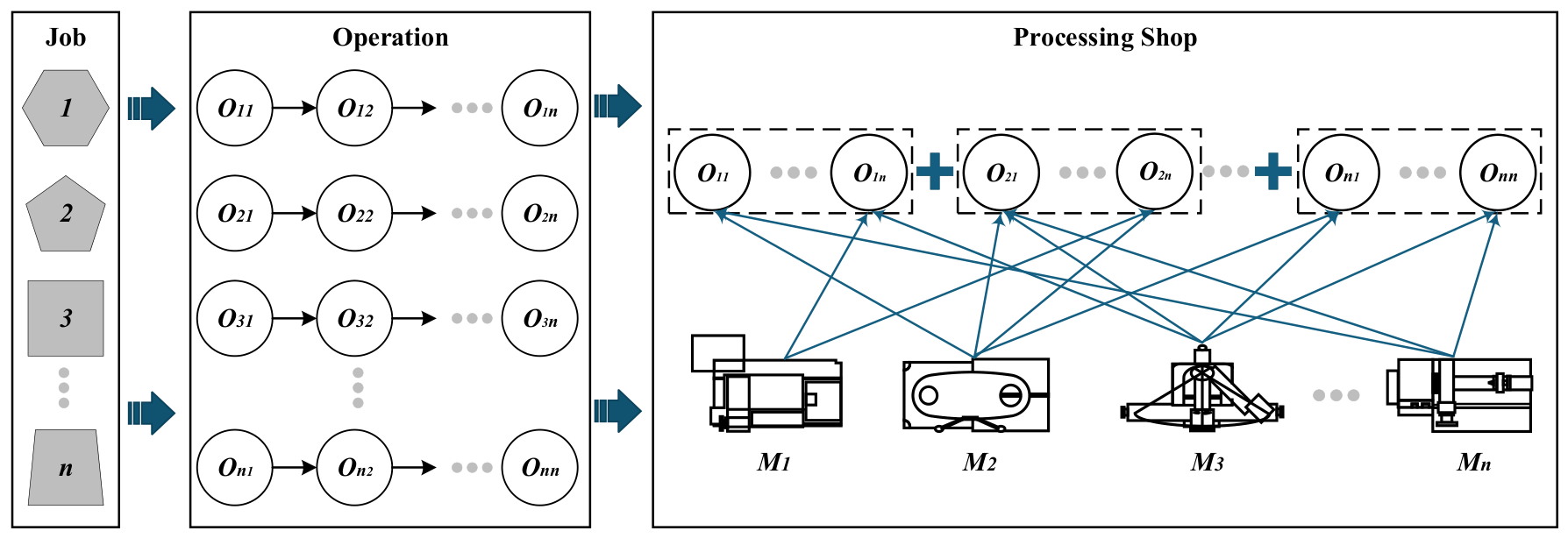
The EA-FJSP is described as follows: There are $n$ jobs that need to be processed on $m$ machines. Each job $j$ consists of $O_i$ operations, where $O_{ij}$ represents the $j$-th operation. Each operation can be processed on one or more compatible machines. The processing time, processing energy consumption, and idle energy consumption of the same operation vary across different machines. The objective of scheduling is to assign suitable machines to each operation and determine the processing sequence of operations on each machine, aiming to minimize the makespan and total energy consumption. Figure 1 intuitively illustrates the production environment of the EA-FJSP.

To facilitate problem modeling, several assumptions are made for the problem considered in this paper, as listed below.

• Each operation of a job should be processed in the sequence of the process route.
• Each machine can process only one operation at a time.
• Each operation can be assigned to only one machine at a time.
• Each operation should not be interrupted when being processed.
• The processing time of each operation depends on the selected machine.
• All jobs are available at the initial time.
• All machines are available at the initial time.

The notations used for the formulation of the EA-FJSP are listed in

Table 2. Notation and description.

Notation	Description
$n$	Number of jobs
$m$	Number of machines
$o_i$	Number of operations in $i$
$i$	Job index
$j$	Operation index
$k$	Machine index
$O_{ij}$	Operation $j$ of job $i$
$O{n}_i$	Next operation to be processed for job $i$
$p_{ijk}$	Processing time of $O_{ij}$ on machine $k$
$M_{ij}$	Available machines set for $O_{ij}$
$S_{ij}$	Start time of $O_{ij}$
$C_{ij}$	Completion time of $O_{ij}$
$C_i$	Completion time of $i$
$E_k^p$	Processing energy consumption of machine $k$ per unit time
$E_k^{idle}$	Idle energy consumption of machine $k$ per unit time
$PE$	Processing energy consumption of the machine during the entire scheduling period
$IE$	The idle energy consumption of the machine during the entire scheduling period
$TE$	Total energy consumption of the machine during the entire scheduling period
$N$	A sufficiently large positive number
$x_{ijk}$	$x_{ijk}=\left\{\begin{array}{c}1 if O_{ij} is assingned to machine k\hfill \\ 0\hspace{1em}\hspace{1em}\hspace{1em}\hspace{1em}otherwise\hfill \end{array}\right.$
$x_{ij{i}^{\prime }{j}^{\prime }k}$	$x_{ij{i}^{\prime }{j}^{\prime }k}=\left\{\begin{array}{c}1 if O_{ij} is a predecessor of O_{i^{\prime }{j}^{\prime }} on machine k\hfill \\ 0\hspace{1em}\hspace{1em}\hspace{1em}\hspace{1em}\hspace{1em}\hspace{1em}otherwise\hfill \end{array}\right.$

.

3.2. EA-FJSP Mathematical Model

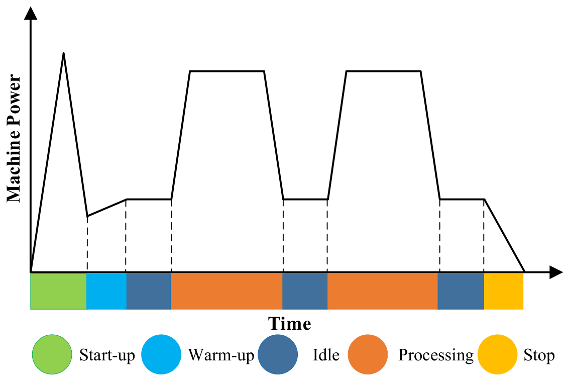
During a complete production cycle, the machine goes through five modes: start-up, warm-up, processing, idle, and stop [34]. The energy consumption in the start-up, warm-up, and stop modes is primarily determined by machine characteristics and is independent of the scheduling policy. In contrast, the processing and idle modes may frequently alternate during the production cycle. Their frequency and duration are directly affected by the scheduling policy. A reasonable scheduling policy can minimize idle time and lower idle energy consumption. It also helps optimize job routing by assigning operations to appropriate machines, thereby minimizing the total processing energy consumption. This paper focuses on machine energy consumption in processing and idle modes and formulates the corresponding EA-FJSP mathematical model. Figure 2 shows the power consumption characteristics of a machine throughout the production cycle.

Based on the description, assumptions, notations, and analysis of energy consumption characteristics, the EA-FJSP mathematical model is formulated as follows.

The objective function:

$$MinF=\min (C_{\max },TE)$$

(1)

where $C_{\max }$ is the makespan objective function.

$$C_{\max }=\max C_i , i=1,2,\dots ,n$$

(2)

$TE$ is the objective function of total energy consumption.

$$TE=PE+IE$$

(3)

where $PE$ is the energy consumption of machines during job processing.

$$PE={\displaystyle \sum _{i=1}^n{\displaystyle \sum _{k=1}^m{\displaystyle \sum _{j=1}^{o_i}{x}_{ijk}\cdot p_{ijk}\cdot E_k^p}}}$$

(4)

$IE$ is the energy consumption when the machine is in idle mode.

$$IE={\displaystyle \sum _{i=1}^n{\displaystyle \sum _{k=1}^m{\displaystyle \sum _{j=1}^{o_i}{x}_{ijk{i}^{\prime }{j}^{\prime }k}}}}\cdot (S_{i^{\prime }{j}^{\prime }k}-C_{ijk})\cdot E_k^{idle}$$

(5)

The EA-FJSP-related constraints are as follows:

$$S_{ij}\ge 0,C_{ij}\ge 0,C_i\ge 0$$

(6)

$$\begin{array}{ccc}{C}_{ij}\ge S_{ij}+p_{ijk}\cdot x_{ijk}& ,& \forall i,j,k\end{array}$$

(7)

$$\begin{array}{ccc}{S}_{ij}\ge C_{i(j-1)}& ,& \forall i,\forall j=2,\dots ,o_i\end{array}$$

(8)

$$S_{i^{\prime }{j}^{\prime }}\ge C_{ij}-N\cdot (1-x_{ij{i}^{\prime }{j}^{\prime }k}),\forall i\ne i^{\prime },j\ne j^{\prime },k\in \left\{1,2,\dots ,m\right\}$$

(9)

$$S_{ij}\ge C_{i^{\prime }{j}^{\prime }}-N\cdot x_{ij{i}^{\prime }{j}^{\prime }k}$$

(10)

$${\displaystyle \sum _{k=1}^m{x}_{ijk}=1},\forall i,j$$

(11)

Equation (6) defines the non-negativity constraints on the start and completion times of operations, as well as the completion time of each job, ensuring that all of these time-related variables take non-negative values. Equation (7) specifies the relationship between the start and completion times of each operation on the assigned machine, indicating that the completion time is determined by the start time and the corresponding processing duration on the selected machine. Equation (8) ensures that the start time of a subsequent operation must be no earlier than the completion time of the preceding operation, thereby strictly maintaining the technological processing sequence within each job. Equations (9) and (10) ensure that two operations assigned to the same machine cannot be processed simultaneously and must be executed in a predefined sequence, thereby preventing any overlap in processing time on the same machine and enforcing machine capacity limitations. Equation (11) ensures that each operation of the same job can only be processed by one machine, guaranteeing a unique machine assignment for each operation.

4. Solving the EA-FJSP Based on DL-PPO

4.1. DL-PPO Hierarchical Scheduling Framework

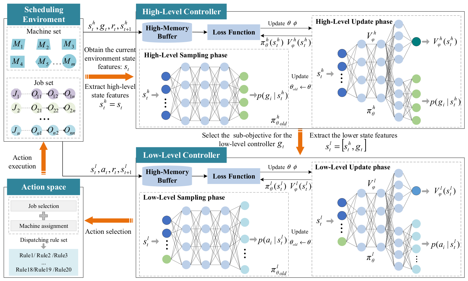
The DL-PPO hierarchical scheduling framework is shown in Figure 3. It consists of three core modules: scheduling environments and a hierarchical controller. The main components are described as follows:

The scheduling environment is the core component of the scheduling framework. It handles interactions between the hierarchical controller and the energy-aware flexible job scheduling system. Its primary functions are to accurately simulate the energy-aware flexible job scheduling process and ensure alignment between scheduling policies and actual production logic. It also provides feedback mechanisms for policy optimization. Specifically, the scheduling environment establishes the operational mechanism of the EA-FJSP to provide accurate state information to the hierarchical controller and receive and execute scheduling decisions in real time. It also provides real-time feedback on changes in job and machine state, thereby effectively responding to actual production requirements and resource constraints.

The hierarchical controller consists of a high-level controller and a low-level controller, each responsible for scheduling decisions at its respective level. The high-level controller employs the PPO algorithm. It includes the high-level sampling phase, high-level update phase, high-level memory buffer, and loss function module. The high-level memory buffer stores relevant data generated during the interactions between the high-level controller and the scheduling environment. This data includes high-level states $s_t^h,s_{t+1}^h$, sub-objectives $g_t$, and reward $r_t$ information. During the high-level update phase, it is used to compute advantage estimates, policy loss, and value function loss. These metrics are then used to optimize the parameters of both the high-level policy network ${\pi }_{\theta }^h$ and the high-level value network $V_{\phi }^h$. The high-level scheduling decision process is divided into the high-level sampling phase and the high-level update phase. During the high-level sampling phase, the high-level controller extracts high-level state features ($s_t^h=s_t$) based on the current state $s_t$. The high-level controller then selects a sub-objective $g_t$ from the set of sub-objectives $G$ through the high-level old policy network ${\pi }_{\theta old}^h$. Here, $G$ represents the set of sub-objectives derived from the decomposition of the global optimization objective. The sub-objective $g_t$ is then passed to the low-level controller to guide its further decision-making. During the high-level training phase, the high-level controller samples data from the high-level memory buffer. It then utilizes the high-level value network $V_{\phi }^h$ to estimate the state value, computes the advantage, and employs the clipping objective function of the PPO algorithm to limit the deviation between the old and new policies during the update process. Finally, the optimized high-level policy network parameters ${\theta }_h$ replace the high-level old policy network parameters ${\theta }_{hold}$, providing support for decision updates in the next round.

The low-level controller is responsible for the selection of feasible dispatching rules according to the selected sub-objectives. It also employs the PPO algorithm, which includes the low-level sampling phase, low-level update phase, low-level memory buffer, and loss function module. The low-level memory buffer stores state features $s_t^l,s_{t+1}^l$, selected dispatching rules $a_t$, and reward $r_t$ information. It provides scheduling data samples for parameter updates of the low-level policy network ${\pi }_{\theta }^l$ and the low-level value network $V_{\phi }^l$. Similar to the high-level controller, the low-level controller is divided into two phases in the scheduling decision process. During the low-level sampling phase, the low-level controller combines the sub-objective $g_t$ selected by the high-level controller with the current state $s_t$ to construct the low-level state features $(s_t^l=[s_t,g_t])$. In accordance with these features, it selects a feasible dispatching rule $a_t$ from the predefined rule set $A$. The selected rule is then applied to the scheduling environment. In the low-level training phase, the low-level controller samples data from the memory buffer to optimize the policy for dispatching rule selection. Finally, the parameters (${\theta }_l$, ${\phi }_l$) of the low-level policy network ${\pi }_{\theta }^l$ and value network $V_{\phi }^l$ are updated by computing the advantage function and employing the clipped objective function in PPO.

By leveraging hierarchical collaboration between the high-level and low-level controllers, continuous interaction with the scheduling environment, and DL-PPO-based scheduling policy optimization at different levels, the high-level controller is able to select an appropriate temporary optimization objective (sub-objective) in accordance with the current state at each decision point. The low-level controller then executes a feasible dispatching rule according to the given sub-objective. This hierarchical framework effectively decomposes the complex EA-FJSP and improves the overall scheduling performance.

In the scheduling framework, the action space consists of a set of dispatching rules that can be executed by the low-level controller. Each rule defines an independent scheduling policy that guides the low-level controller in making optimal scheduling decisions during the energy-aware flexible job shop scheduling process. These rules are tailored to specific energy-aware scheduling scenarios and optimization objectives, encompassing various scheduling policies. The goal is to improve the overall scheduling performance by considering production efficiency and energy consumption.

4.2. Multi-Dimensional State Features

In DL-PPO, state features serve as inputs to neural networks within both the high-level and low-level controllers, providing support for scheduling decisions at different levels. These features need to accurately and intuitively reflect the scheduling information at different times while uniformly characterizing the scheduling environments. This ensures that the algorithm has a high degree of adaptability and effectiveness in complex environments. Based on this goal, state features are extracted from four dimensions: job, machine, time, and energy consumption. Twelve representative state features are designed. The combination of these state features reflects scheduling information from different dimensions, providing a comprehensive representation of the scheduling environment. The definitions and calculation formulas for each state feature are as follows.

• Job Dimension:
  • The average number of remaining operations for all jobs $RN{O}_{ave}$, which is used to measure the overall progress of job processing.

    $$RN{O}_{ave}(t)={\displaystyle \frac{1}{n}}{\displaystyle \sum _{i=1}^n(o_i-{\displaystyle \sum _{j=1}^{o_i}{x}_{ijk}})}$$

    (12)
  • The average completion rate of jobs $JC{R}_{ave}$, which is used to reflect the degree of completion in job processing.

    $$JC{R}_{ave}(t)={\displaystyle \frac{1}{n}}{\displaystyle \sum _{i=1}^n\left({\displaystyle \sum _{j=1}^{o_i}{x}_{ijk}\cdot \frac{1}{o_i}}\right)}$$

    (13)
  • The standard deviation of the job completion rate $JC{R}_{ave}^{std}$, which is used to evaluate the uniformity and stability of job processing.

    $$JC{R}_{ave}^{std}(t)=\sqrt{{\displaystyle \frac{1}{n}}{\displaystyle \sum _{i=1}^n({\displaystyle \sum _{j=1}^{o_i}{x}_{ijk}}\cdot \frac{1}{o_i}-JC{R}_{ave}{(t))}^2}}$$

    (14)
• Machine Dimension:

  4.

  The standard deviation of machine load $M{L}_{ave}^{std}$, which is used to reflect the uniformity of machine resource allocation.

  $$M{L}_{ave}^{std}(t)=\sqrt{{\displaystyle \frac{1}{m}}{\displaystyle \sum _{k=1}^m{\left(\left({\displaystyle \sum _{i=1}^n{\displaystyle \sum _{j=1}^{o_i}{x}_{ijk}\cdot p_{ijk}}}\right)-\frac{1}{m}{\displaystyle \sum _{k=1}^m{\displaystyle \sum _{i=1}^n{\displaystyle \sum _{j=1}^{o_i}{x}_{ijk}\cdot p_{ijk}}}}\right)}^2}}$$

  (15)

  5.

  The average utilization rate of machines $U_{ave}$, which is used to reflect the efficiency of machine resource usage.

  $$U_{ave}(t)={\displaystyle \frac{1}{m}}{\displaystyle \sum _{k=1}^m\left({\displaystyle \sum _{i=1}^n{\displaystyle \sum _{j=1}^{o_i}{x}_{ijk}{p}_{ijk}}\cdot \frac{1}{\max C_i(t)}}\right)}$$

  (16)

  6.

  The standard deviation of machine utilization rate $U_{ave}^{std}$, which is used to measure the balance in the machine utilization distribution.

  $$U_{ave}^{std}(t)=\sqrt{{\displaystyle \frac{1}{m}}{\displaystyle \sum _{k=1}^m({\displaystyle \sum _{i=1}^n{\displaystyle \sum _{j=1}^{o_i}{x}_{ijk}\cdot p_{ijk}}}\cdot \frac{1}{\max C_i(t)}-U_{ave}{(t))}^2}}$$

  (17)

• Time Dimension

  7.

  The maximum completion time of jobs $JC{T}_{\max }$ at time $t$, which is used to reflect the current makespan in the production schedule.

  $$JC{T}_{\max }(t)=\begin{array}{cc}\max C_i(t),& i=1,2,\dots ,n\end{array}$$

  (18)

  8.

  The estimated maximum completion time of jobs $EJC{T}_{\max }$ at time $t$, which is used to measure the upper bound of the expected makespan for the entire schedule.

  $$\begin{array}{cc}EJC{T}_{\max }(t)=\max \left[{\displaystyle \sum _{i=O{n}_i}^{o_i}\left({\displaystyle \sum _{M_k\in M_{ij}}{p}_{ijk}\cdot \frac{1}{\left|M_{ij}\right|}}\right)+C_i(t)}\right]& i=1,2,\dots ,n\end{array}$$

  (19)

  9.

  The ratio between the estimated maximum completion time of the remaining jobs and that of all jobs $RJCT$ at time $t$, which is used to measure the relative progress of the remaining jobs in comparison with the overall scheduling process.

  $$\begin{array}{ccc}RJCT(t)=& {\displaystyle \frac{\max ({\displaystyle \sum _{j=O{n}_i}^{o_i}\frac{{\displaystyle \sum _{M_k\in M_{ij}}{p}_{ijk}}}{\left|M_{ij}\right|})}}{EJC{T}_{\max }(t)}},& i=1,2,\dots ,n\end{array}$$

  (20)

• Energy Consumption Dimension:

  10.

  The total energy consumption of the machines $MTEC$, which is used to reflect their current overall energy consumption level.

  $$MTEC(t)={\displaystyle \sum _{k=1}^m{\displaystyle \sum _{i=1}^n{\displaystyle \sum _{j=1}^{o_i}(x_{ijk}\cdot p_{ijk}\cdot E_k^p+x_{ijk{i}^{\prime }{j}^{\prime }k}\cdot (S_{i^{\prime }{j}^{\prime }k}-C_{ijk})\cdot E_k^{idle})}}}$$

  (21)

  11.

  The total energy consumption expected to be generated by the machines for processing the remaining operations $ROEC$, which is used to estimate the energy consumption demand of these operations.

  $$ROEC(t)={\displaystyle \sum _{i=1}^n{\displaystyle \sum _{j=O{n}_i}^{o_i}{\displaystyle \sum _{M_k\in M_{ij}}{p}_{ijk}\cdot E_k^p}}}\cdot {\displaystyle \frac{1}{\left|M_{ij}\right|}}$$

  (22)

  12.

  The ratio of the total energy consumption expected to be generated by the machines for processing the remaining operations to the total expected energy consumption of the machines $ROMT$, which is used to measure the proportion of the energy consumption demand of the remaining tasks relative to the total.

  $$ROMT(t)={\displaystyle \frac{ROEC(t)}{ROEC(t)+MTEC(t)}}$$

  (23)

To avoid shortsightedness and promote global optimality, DL-PPO adopts a hierarchical decision-making mechanism. The high-level controller captures the global production state based on state features extracted from four dimensions, i.e., job, machine, time, and energy, and uses this information to guide the long-term optimization direction while selecting a temporary optimization objective. The low-level controller takes both the current state features and the selected objective as input and determines the feasible dispatching rule accordingly. In this way, the dynamic interaction between global state information and objective selection jointly determines the final scheduling decision, enabling adaptive rule selection under different production conditions. Specifically, the input features of the high-level controller are represented as:

$$s_t^h=\left\{RN{O}_{ave}(t),JC{R}_{ave}(t),\dots ,ROMT(t)\right\}$$

The input features of the low-level controller are represented as:

$$s_t^l=\left\{RN{O}_{ave}(t),JC{R}_{ave}(t),\dots ,ROMT(t),g_t\right\}$$

4.3. Action Space

In the scheduling process, the action space of the low-level controller refers to a set of dispatching rules executable at each decision step. These rules are used to dynamically adjust the scheduling environment and advance the scheduling process. In addition, compared to the traditional job shop scheduling problem, the EA-FJSP exhibits greater flexibility. Specifically, each operation of a job can be processed by multiple machines that meet the processing requirements. Each decision step in this process involves two decision points: job selection and machine assignment. To enhance scheduling flexibility and achieve optimal scheduling policies in both time and energy consumption dimensions, twenty dual-decision-point dispatching rules are designed as the action space for the low-level controller. These rules aim to comprehensively cover the corresponding scheduling scenarios and adapt to complex optimization requirements.

Table 3. Dual-decision-point dispatching rules.

Index	Job Selection Rule	Machine Assignment Rule	Index	Job Selection Rule	Machine Assignment Rule
1	SRPT	LECM	11	FOR	SPT
2	SRPT	HECM	12	FOR	LPT
3	LRPT	LECM	13	LREC	SPT
4	LRPT	HECM	14	LREC	LPT
5	LCPT	LECM	15	HREC	SPT
6	LCPT	HECM	16	HREC	LPT
7	SCPT	LECM	17	HCEC	SPT
8	SCPT	HECM	18	HCEC	LPT
9	MOR	SPT	19	LCEC	SPT
10	MOR	LPT	20	LCEC	LPT

Note: SRPT: selecting the job with the shortest remaining processing time; LRPT: selecting the job with the longest remaining processing time; LCPT: selecting the job with the longest current processing time; SCPT: selecting the job with the shortest current processing time; MOR: selecting the job with the most operations remaining; FOR: selecting the job with the fewest operations remaining; LREC: selecting the job with the lowest remaining processing energy consumption; HREC: selecting the job with the highest remaining processing energy consumption; HCEC: selecting the job with the highest current processing energy consumption; LCEC: selecting the job with the lowest current processing energy consumption; LECM: assigning the machine with the lowest processing energy consumption; HECM: assigning the machine with the highest processing energy consumption; SPT: assigning the machine with the shortest processing time; LPT: assigning the machine with the longest processing time.

presents the twenty dual-decision-point dispatching rules and their descriptions.

4.4. Sub-Objective

The collaborative optimization of makespan and total energy consumption in EA-FJSP remains a challenging problem due to the complex interactions among flexible routing, machine states, and energy consumption characteristics. Therefore, the global optimization objective is decomposed into different dimensions to better address the diverse requirements of scheduling. Four targeted sub-objectives $g\in (1,2,3,4)$ are designed to construct the high-level decision-making system. The four sub-objectives are machine utilization $U_{ave}$, the inverse of the maximum job completion time $C_{\max }^{-1}$, the variation ratio of energy consumption $E_{pre}^{now}$, and the uniformity of energy consumption distribution $E_{\max }^{mean}$. These sub-objectives help balance scheduling policies across multiple dimensions, thereby improving the overall optimization performance. The design and meaning of the four sub-objectives are as follows.

Machine utilization $U_{ave}$: the average utilization rate of machines. Maximizing this rate reduces machine idle time and increases workload saturation. This indirectly optimizes energy consumption and enhances overall scheduling efficiency.

$$U_{ave}(t)={\displaystyle \frac{1}{m}}\cdot {\displaystyle \sum _{k=1}^m{U}_k(t)}$$

(24)

where $U_k$ is the utilization of machine $k$.

$$\begin{array}{cc}{U}_k(t)={\displaystyle \frac{{\displaystyle \sum _{i=1}^n{\displaystyle \sum _{j=1}^{o_i}{x}_{ijk}\cdot p_{ijk}}}}{\max C_i(t)}},& k=1,2,\dots ,m\end{array}$$

(25)

The inverse of the maximum job completion time $C_{\max }^{-1}$: refers to the completion time of the last completed job among all jobs at time $t$, which is expressed as its reciprocal. Optimizing this metric can shorten the makespan and improve scheduling efficiency.

$$\begin{array}{cc}{C}_{\max }^{-1}(t)={\displaystyle \frac{1}{\max C_i(t)}},& i=1,2,\dots ,n\end{array}$$

(26)

where, to avoid division by zero, the value of $C_{\max }^{-1}$ is initialized to 0 at the beginning.

The variation ratio of energy consumption $E_{pre}^{now}$: the ratio of the total energy consumption expected to be generated by machines at time $t$ to the total energy consumption expected in the unscheduled state. It evaluates the effectiveness of the current scheduling policy in optimizing energy consumption. Optimizing this ratio allows the evaluation of the effectiveness of the scheduling policy in reducing energy consumption while satisfying task constraints.

$$E_{pre}^{now}(t)={\displaystyle \frac{E_k^{all}(t)+E_i^{no}(t)}{E^{pre}}}$$

(27)

where $E_k^{all}$ is the total energy generated by all machines at time $t$.

$$E_k^{all}(t)={\displaystyle \sum _{k=1}^m{\displaystyle \sum _{i=1}^n{\displaystyle \sum _{j=1}^{o_i}(x_{ijk}\cdot p_{ijk}\cdot E_k^p+x_{ijk{i}^{\prime }{j}^{\prime }k}\cdot (S_{i^{\prime }{j}^{\prime }k}-C_{ijk})\cdot E_k^{idle})}}}$$

(28)

$E_i^{no}$ is the estimated total energy consumption required for the machines to process the remaining operations.

$$E_i^{no}(t)={\displaystyle \sum _{i=1}^n{\displaystyle \sum _{j=O{n}_i}^{o_i}\frac{{\displaystyle \sum _{M_k\in M_{ij}}{p}_{ijk}\cdot E_k^p}}{\left|M_{ij}\right|}}}$$

(29)

$E^{pre}$ is the estimated total energy consumption of the machines in the unscheduled state.

$$E^{pre}={\displaystyle \sum _{i=1}^n{\displaystyle \sum _{j=1}^{o_i}\frac{{\displaystyle \sum _{M_k\in M_{ij}}{p}_{ijk}\cdot E_k^p}}{\left|M_{ij}\right|}}}$$

(30)

The uniformity of energy consumption distribution $E_{\max }^{mean}$: the ratio between the maximum energy consumption and the average energy consumption among all machines at time $t$. It measures the disparity between the highest and the average machine energy consumption. This ratio helps evaluate the balance of energy consumption across machines, optimizes resource allocation, and improves overall energy efficiency.

$$E_{\max }^{mean}(t)={\displaystyle \frac{\frac{1}{m}{E}_k^{all}(t)}{\max E_k(t)}}$$

(31)

where $E_k$ is the current total energy consumption of each machine at time $t$.

$$E_k(t)=\begin{array}{cc}{\displaystyle {\displaystyle \sum _{i=1}^n}{\displaystyle \sum _{j=1}^{o_i}{x}_{ijk}\cdot p_{ijk}\cdot E_k^p+}}{\displaystyle {\displaystyle \sum _{i=1}^n}{\displaystyle \sum _{j=1}^{o_i}{x}_{ijk{i}^{\prime }{j}^{\prime }k}}}\cdot (S_{i^{\prime }{j}^{\prime }k}-C_{ijk})E_k^{idle},& k=1,2,\dots ,m\end{array}$$

(32)

With the four sub-objectives, the high-level controller can dynamically evaluate the scheduling environment at each decision step. By analyzing the impact of time and energy consumption on the current scheduling environment from different dimensions, it adaptively selects the most influential sub-objective as the optimization objective for the current phase. The high-level controller guides the low-level controller to select feasible dual-decision-point dispatching rules at the local optimization level, thus achieving goal-driven scheduling optimization. At the same time, this method takes into account both short-term gains and long-term scheduling stability, enhancing the adaptability and efficiency of the algorithm.

4.5. Reward Function

To ensure that the cumulative reward in the scheduling process is consistent with the optimization direction of the global objectives while alleviating the issue of sparse rewards, the reward function is designed to be closely related to the sub-objectives at each decision step. At decision time step $t$, the high-level controller dynamically selects a sub-objective according to the current system state $s_t$. Based on the selected sub-objective, a corresponding reward function is activated to guide the optimization process. Subsequently, the low-level controller executes the selected dual-decision-point dispatching rule, which drives the system to transition from state $s_t$ to state $s_{t+1}$. The reward is then determined by evaluating the variation of the selected sub-objective before and after the state transition. Specifically, the reward is calculated according to whether the selected sub-objective is improved at time step $t+1$ compared with its value at time step $t$, thereby providing immediate feedback to the learning agent.

To meet the optimization requirements of different sub-objectives, four corresponding reward functions are designed. These reward functions are evaluated from the four dimensions of $U_{ave}$, $C_{\max }^{-1}$, $E_{pre}^{now}$, and $E_{\max }^{mean}$, respectively. Each reward function is formulated to reflect the local improvement in its associated sub-objective, thereby enhancing the effectiveness and stability of the hierarchical learning process. The specific forms are as follows:

At time $t$, if the sub-objective $g_t=1$ is selected, $U_{ave}(t)$ and $U_{ave}(t+1)$ are selected as the reward indicators. The $r_t$ is calculated according to Equation (33).

$$r_t=\left\{\begin{array}{cc}1,& U_{ave}(t)<U_{ave}(t+1)\\ 0,& U_{ave}(t)=U_{ave}(t+1)\\ -1,& U_{ave}(t)>U_{ave}(t+1)\end{array}\right.$$

(33)

At time $t$, if the sub-objective $g_t=2$ is selected, $C_{\max }^{-1}(t)$ and $C_{\max }^{-1}(t+1)$ are selected as the reward indicators. The $r_t$ is calculated according to Equation (34).

$$r_t=\left\{\begin{array}{cc}1,& C_{\max }^{-1}(t)\le C_{\max }^{-1}(t+1)\\ -1,& C_{\max }^{-1}(t)>C_{\max }^{-1}(t+1)\end{array}\right.$$

(34)

At time $t$, if the sub-objective $g_t=3$ is selected, $E_{pre}^{now}(t)$ and $E_{pre}^{now}(t+1)$ are selected as the reward indicators. The $r_t$ is calculated according to Equation (35).

$$r_t=\left\{\begin{array}{cc}1,& E_{pre}^{now}(t)>E_{pre}^{now}(t+1)\\ 0,& E_{pre}^{now}(t)=E_{pre}^{now}(t+1)\\ -1,& E_{pre}^{now}(t)<E_{pre}^{now}(t+1)\end{array}\right.$$

(35)

At time $t$, if the sub-objective $g_t=4$ is selected, $E_{\max }^{mean}(t)$ and $E_{\max }^{mean}(t+1)$ are selected as the reward indicators. The $r_t$ is calculated according to Equation (36).

$$r_t=\left\{\begin{array}{cc}1,& E_{\max }^{mean}(t)<E_{\max }^{mean}(t+1)\\ 0,& E_{\max }^{mean}(t)=E_{\max }^{mean}(t+1)\\ -1,& E_{\max }^{mean}(t)>E_{\max }^{mean}(t+1)\end{array}\right.$$

(36)

The four reward functions effectively guide the scheduling optimization process toward the optimization directions of sub-objectives. They also continuously motivate the low-level controller to take favorable actions during state transitions. This enables effective coordination between local and global optimization, enhancing the adaptability and convergence efficiency of the scheduling policy.

4.6. DL-PPO Training Process

During training, the scheduling environment and the scheduling state are first initialized. Then, the system enters the scheduling decision loop. At each scheduling decision point, the high-level controller extracts high-level state features $s_t^h=s_t$ from the current state $s_t$ and selects a sub-objective $g_t$ through the high-level old policy network ${\pi }_{\theta old}^h$. This sub-objective then guides the low-level controller to make low-level scheduling decisions. The low-level controller takes the selected sub-objective $g_t$ and the current state $s_t$ as low-level state features $s_t^l=[s_t,g_t]$. It utilizes the low-level old policy network ${\pi }_{\theta old}^l$ to select a feasible dual-decision-point dispatching rule. After executing the action, the environment returns a reward $r_t$ and updates the scheduling state $s_{t+1}$. The high-level and low-level states are then updated accordingly.

In DL-PPO, the high-level and low-level memory buffers store their respective interaction data with the scheduling environment. When the memory buffer reaches the predefined threshold, the high-level and low-level discounted returns and advantage functions are calculated. The algorithm is employed to update the parameters of the policy and value networks, enabling the iterative optimization of both high-level and low-level policy networks. Finally, the optimized policy is applied to guide the energy-aware flexible job shop scheduling process. The objective is to achieve collaborative optimization of energy consumption and makespan. The complete training process of the DL-PPO is shown in Algorithm 1.

Algorithm 1. The training process of DL-PPO.
	Input: policy network ${\pi }_{\theta }^h,$ ${\pi }_{\theta }^l$ and value network $V_{\phi }^h,$ $V_{\phi }^l$ with trainable parameters ${\theta }_h$ ${\theta }_{hold},$ ${\theta }_l,$ ${\theta }_{lold},$ ${\phi }_h,$ ${\phi }_l.$ Learning rates $\alpha$, discount factor $\gamma$, memory buffer size $M^h,$ $M^l,$ update epochs $K$, PPO clipping factor $\epsilon$, training cycles $L$.
	Output: Trained policy network ${\pi }_{\theta }^h,$ ${\pi }_{\theta }^l$ and experimental results.
1:	for cycle < $L$ do
2:	Reset the energy-aware flexible job shop scheduling environment.
3:	Initialize $s_0.$
4:	while scheduling is not finished, do
5:	Extract high-level state features $s_t^h=s_t.$
6:	Use ${\pi }_{\theta old}^h$ to select sub-objective $g_t~{\pi }_{\theta old}^h(g|s_t^h).$
7:	Extract low-level state features $s_t^l=[s_t,g_t].$
8:	Use ${\pi }_{\theta old}^l$ to select action $a_t~{\pi }_{\theta old}^l(a|s_t^l).$
9:	Execute $a_t,$ receive reward $r_t$ and update scheduling state $s_{t+1}$
10:	Update high-level state features $s_{t+1}^h=s_{t+1}.$
11:	Use ${\pi }_{\theta old}^h$ to select sub-objective $g_{t+1}~{\pi }_{\theta old}^h(g|s_{t+1}^h).$
12:	Update low-level state features $s_{t+1}^l=[s_{t+1},g_{t+1}].$
13:	Store $(s_t^h,g_t,r_t,s_{t+1}^h)$ in high-level memory buffer $D_h.$
14:	Store $(s_t^l,a_t,r_t,s_{t+1}^l)$ in low-level memory buffer $D_l.$
15:	end while
16:	if $\left|D_h\right|\ge M^h$ then
17:	Compute return $R_t$ for each step using discount factor $\gamma$
18:	Compute advantage function $A_t^h.$
19:	for epoch < $K$ do
20:	Update the policy network parameters ${\theta }_h$ using gradient ascent based on PPO objective.
21:	Update the value network parameters ${\phi }_h.$
22:	end for
23:	Update ${\pi }_{\theta old}^h\leftarrow {\pi }_{\theta }^h$
24:	end if
25:	if $\left|D_l\right|\ge M^l$ then
26:	Compute return $R_t$ for each step using discount factor $\gamma$
27:	Compute advantage function $A_t^l.$
28:	for epoch < $K$ do
29:	Update the policy network parameters ${\theta }_l$ using gradient ascent based on PPO objective.
30:	Update the value network parameters ${\phi }_l$
31:	end for
32:	Update ${\pi }_{\theta old}^l\leftarrow {\pi }_{\theta }^l$
33:	end if
34:	end for

5. Numerical Experiments

5.1. Parameter Settings

The experiments are conducted on a PC with an Intel Core i9-14900HX CPU, using Python and the PyTorch framework, and the development environment is PyCharm Community Edition 2020.1.3 (x64). In DL-PPO, both the high-level and low-level controllers employ the PPO algorithm. The policy network and value network are respectively responsible for decision-making and value estimation. The policy network extracts state features through fully connected layers. It first generates unnormalized actions, which are then transformed into a probability distribution via the softmax function for sampling. The value network adopts a similar structure and outputs a single scalar representing the state value estimate. The neural networks of both the high-level and low-level controllers consist of one input layer, three hidden layers, and one output layer.

All neural network parameters are updated using the Adam optimizer to improve training efficiency and stability. The specific parameter settings are shown in

Table 4. Parameter settings of the DL-PPO.

Parameter	Value
Training cycles	3000
Policy network learning rate	0.004
Value network learning rate	0.004
Clipping parameter	0.1
Discount rate	0.9
High-level batch size	32
Low-level batch size	128
Update epochs	10

. Specifically, the selection of these parameters is based on a combination of empirical analysis, prior studies on PPO-based scheduling methods, and preliminary tuning experiments on representative scheduling instances. In particular, the parameter configuration considers the characteristics of hierarchical decision-making, the complexity of the scheduling environment, and the stability requirements of policy optimization. In DL-PPO, the high-level controller is responsible for macro-level strategy and sub-objective selection, featuring a relatively small decision space; therefore, its batch size is set to 32 to ensure stable and efficient learning. In contrast, the low-level controller handles job selection and machine assignment with a larger action space and higher decision complexity, and its batch size is set to 128 to improve state coverage and learning stability. This hierarchical configuration facilitates effective coordination between local sub-objective optimization and global scheduling performance. For the remaining parameters, both the policy and value networks adopt a learning rate of 0.004 to balance convergence speed and stability. The PPO clipping parameter is set to 0.1 to constrain policy updates and prevent instability, while the discount factor is set to 0.9 to balance short-term and long-term rewards in sequential decision-making. In addition, the number of update epochs is set to 10 to enhance sample efficiency without causing overfitting, and the total number of training cycles is set to 3000 to ensure sufficient exploration and convergence in the complex scheduling environment.

5.2. Performance Metrics

Experiments are conducted using benchmark instances provided by Benchmark [58]. Since these instances do not originally account for machine energy consumption, an energy-aware extension is introduced by incorporating both processing and idle energy components into the model. Specifically, for each machine, two types of power parameters are defined: processing power and idle power. The processing power represents the energy consumption rate when the machine is actively executing an operation, while the idle power corresponds to the energy consumed when the machine is not processing but remains operational. To simulate heterogeneous energy characteristics across machines, these parameters are randomly generated using a uniform distribution. For all MK benchmark instances, the processing power is sampled from the range [1,5], and the idle power is sampled from the range [0.1, 1]. Furthermore, the total energy consumption of each machine is calculated based on the scheduling results, including both processing energy and idle energy over the entire scheduling horizon. The processing energy is determined by the product of processing power and operation duration, while the idle energy is computed according to the machine idle time multiplied by its idle power.

This study addresses the EA-FJSP, aiming to minimize both the makespan and total energy consumption. The goal is to find a set of Pareto-optimal solutions uniformly distributed in the Pareto-optimal front. To comprehensively evaluate the quality of the obtained Pareto-optimal solutions, five performance metrics are adopted. These include Average Makespan ($C_{\max }^{ave}$), Average Total Energy Consumption of Machines ($T{E}^{ave}$), Generational Distance (GD), Inverted Generational Distance (IGD), and Spread ($\Delta$). Specifically, the $C_{\max }^{ave}$ metric evaluates the ability of scheduling algorithms to minimize the makespan, with smaller values indicating better optimization performance. The $A{E}^{ave}$ metric evaluates the ability of scheduling algorithms to minimize the total machine energy consumption, with smaller values indicating that the algorithm performs better in optimizing total energy consumption. The GD and $\Delta$ metrics evaluate the convergence and diversity of the obtained Pareto-optimal solutions, respectively, with smaller values indicating better convergence and diversity. The IGD metric provides a more comprehensive evaluation. It reflects both the convergence and diversity of the solution set, with smaller values indicating better performance. The definitions of these five metrics are listed as follows.

Efficiency metric: Average makespan.

$$C_{\max }^{ave}={\displaystyle \frac{1}{N}}{\displaystyle \sum _{i=1}^N\min C_{\max }^i}$$

(37)

where $N$ is the number of training times, $C_{\max }^i$ is the makespan in the $i$-th training.

Energy consumption metric: Average total energy consumption of machines.

$$T{E}^{ave}={\displaystyle \frac{1}{N}}{\displaystyle \sum _{i=1}^N\min T{E}^i}$$

(38)

where $A{E}^i$ is the total energy consumption of machines in the $i$-th training.

Convergence metric: Generational Distance.

$$GD(A,P)={\displaystyle \frac{1}{\left|A\right|}}\cdot \sqrt{{\displaystyle {\sum }_{i=1}^{\left|A\right|}{d}_{i,A,P}^2}}$$

(39)

where $P$ is the true Pareto-optimal front of an optimization problem and $A$ is the approximate Pareto-optimal front obtained by the algorithm to be evaluated. $d_{i,A,P}$ is the Euclidean distance between the $i$-th solution in $A$ and its closest neighbor in $P$.

Comprehensive metric: Inverse Generational Distance.

$$IGD(P,A)={\displaystyle \frac{1}{\left|P\right|}}{\displaystyle \sum _{i=1}^{\left|P\right|}{d}_{i,P,A}}$$

(40)

where $d_{i,P,A}$ is the Euclidean distance between the $i$-th solution in $P$ and its closest neighbor in $A$.

Diversity metric: Spread.

$$\Delta ={\displaystyle \frac{{\displaystyle {\displaystyle \sum _{j=1}^{N_O}}{d}_{j,A,p}^e}+{\displaystyle {\displaystyle \sum _{i=1}^{\left|A\right|}}\left|d_{i,A,A}-{\overline{d}}_{A,A}\right|}}{{\displaystyle \sum _{j=1}^{N_O}{d}_{j,A,p}^e}+\left|A\right|\cdot {\overline{d}}_{A,A}}}$$

(41)

where $d_{i,A,A}$ is the Euclidean distance of the $i$-th solution in $A$ to its closest neighbor in $A$, and ${\overline{d}}_{A,A}$ is the average value of all $d_{i,A,A}$. $d_{j,A,P}^e$ is the Euclidean distance between the extreme solution of $A$ and the boundary solution of $P$ with regard to the $j$-th objective. $N_O$ is the number of objectives.

Because the true Pareto-optimal front $P$ is unknown, all Pareto-optimal solutions obtained from multiple independent runs of DL-PPO and other comparison methods are first aggregated in the comparative experiments. Then, the non-dominated solutions are selected to construct $P$. This method improves the approximation accuracy of $P$ with respect to the true Pareto front. It also ensures the representativeness and robustness of the solution set in performance evaluation, making it a reliable benchmark for comparative analysis.

5.3. Comparisons with Dispatching Rules

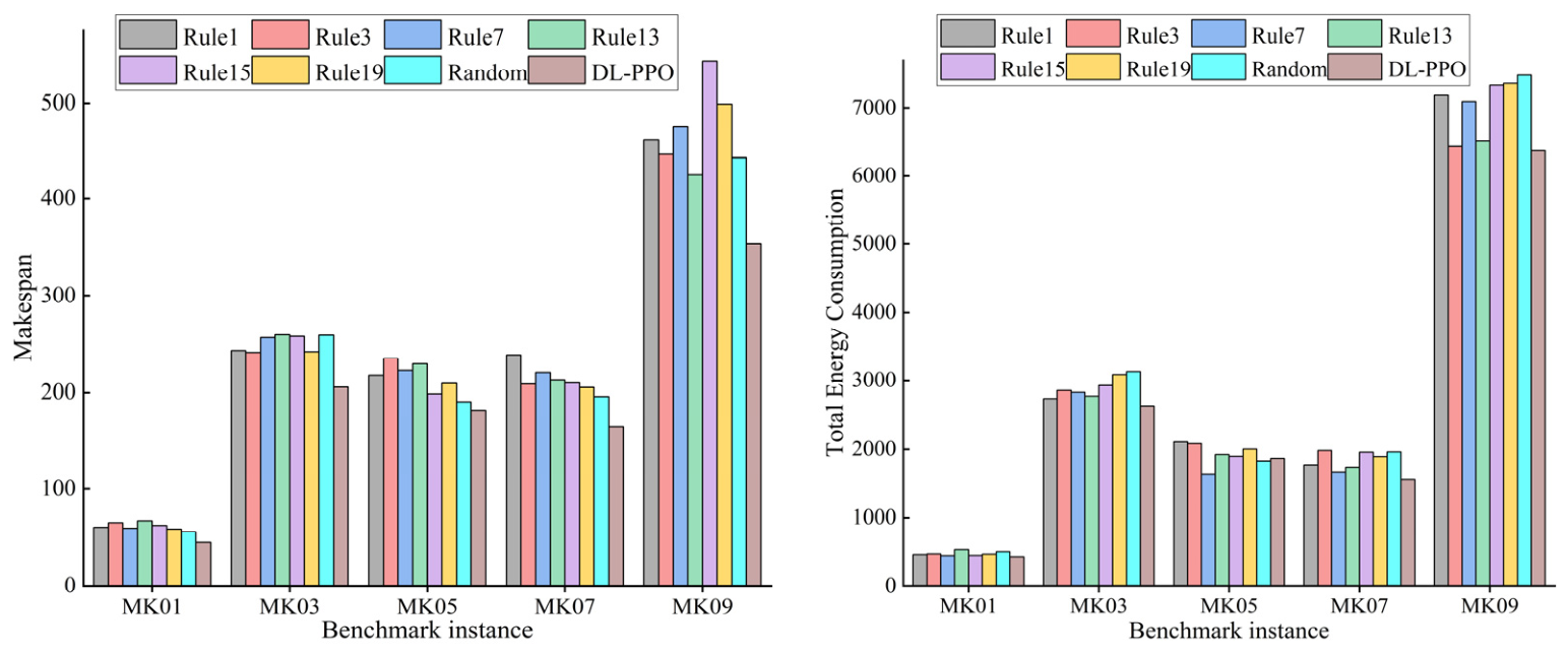
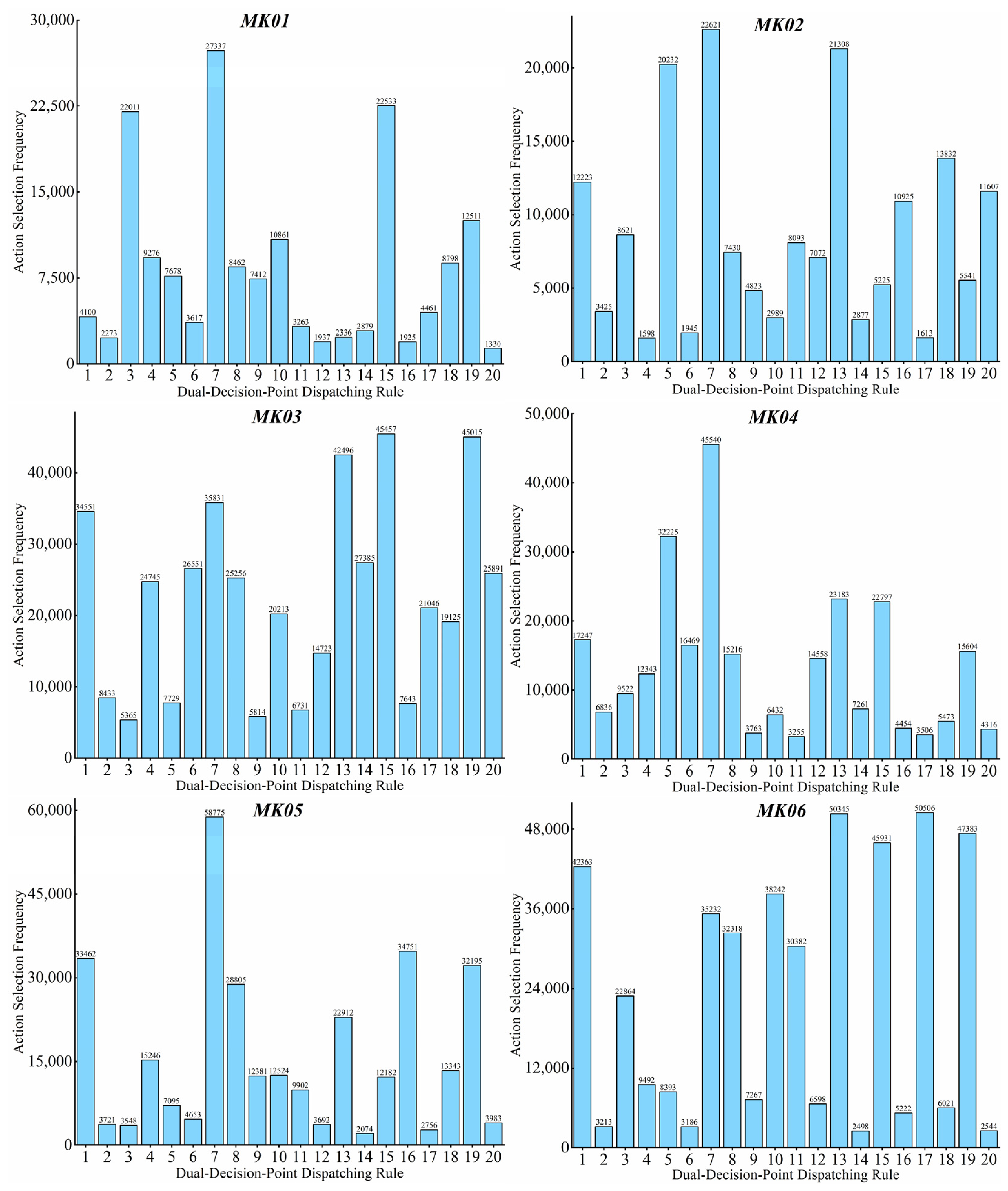
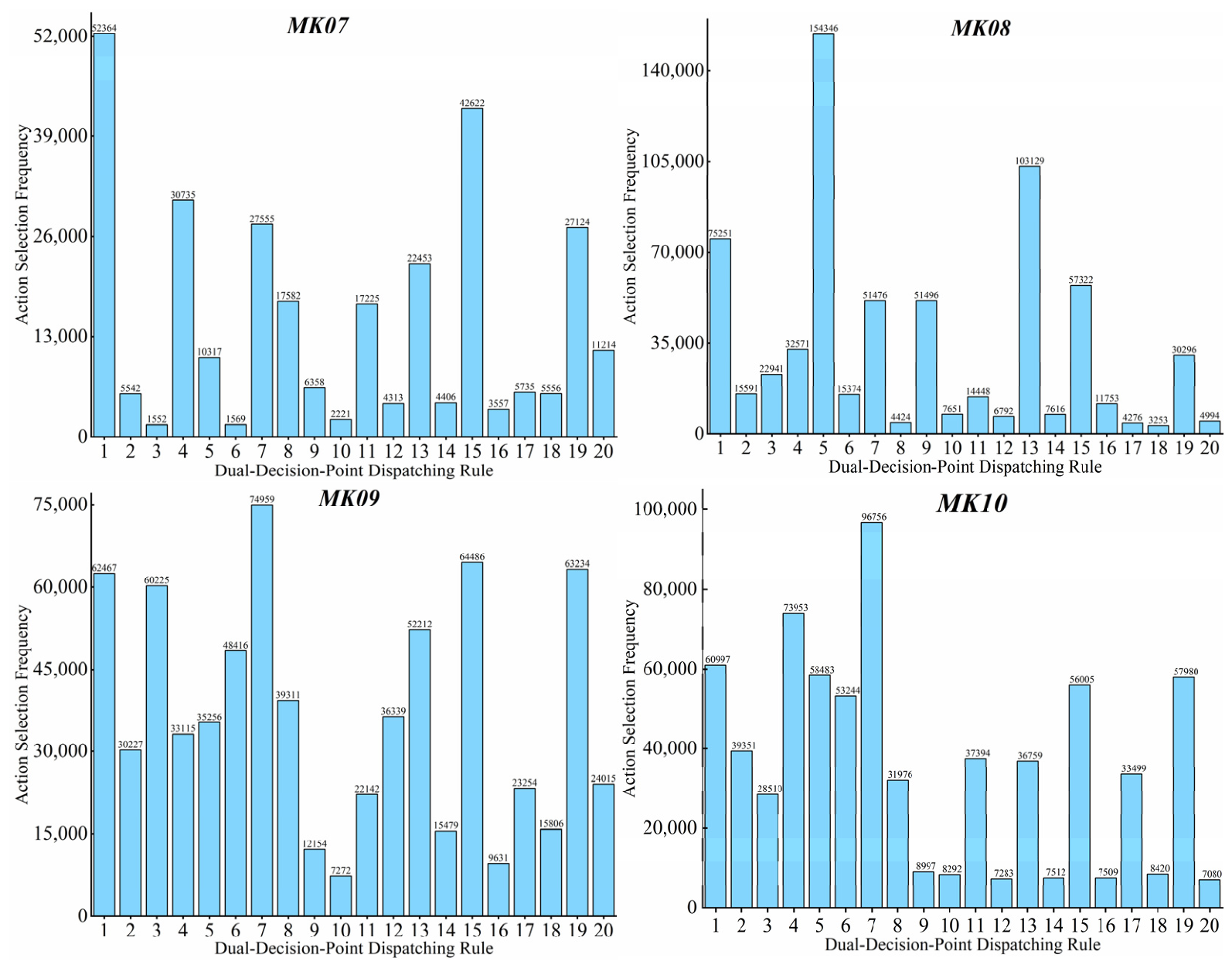
The experiments compare DL-PPO with the proposed dual-decision-point dispatching rules. Based on the training performance of the algorithm on all MK benchmark instances, six frequently used dual-decision-point dispatching rules are selected for comparison. The usage frequency of each dual-decision-point dispatching rule is statistically analyzed, as shown in Figure 4.

To further evaluate the ability of the hierarchical controller to learn and execute effective policies at different decision levels, a random policy (Random) is introduced for comparison. Specifically, at each decision point, the high-level and low-level controllers randomly select a sub-objective and a dual-decision-point dispatching rule, respectively. To ensure the reliability of the results, each method is run 10 times independently on each benchmark instance. The $C_{\max }^{ave}$, $T{E}^{ave}$, GD, IGD, and $\Delta$ obtained from different methods on each benchmark instance are calculated and compared. The comparative results are shown in

Table 5. $C_{\max }^{ave}$ obtained by DL-PPO and dual-decision-point dispatching rules.

Benchmark Instance	Scale	Best Known Solution Range	Rule1	Rule3	Rule7	Rule13	Rule15	Rule19	Random	DL-PPO
			${\mathit{C}}_{\mathbf{max}}^{\mathit{a}\mathit{v}\mathit{e}}$	${\mathit{C}}_{\mathbf{max}}^{\mathit{a}\mathit{v}\mathit{e}}$	${\mathit{C}}_{\mathbf{max}}^{\mathit{a}\mathit{v}\mathit{e}}$	${\mathit{C}}_{\mathbf{max}}^{\mathit{a}\mathit{v}\mathit{e}}$	${\mathit{C}}_{\mathbf{max}}^{\mathit{a}\mathit{v}\mathit{e}}$	${\mathit{C}}_{\mathbf{max}}^{\mathit{a}\mathit{v}\mathit{e}}$	${\mathit{C}}_{\mathbf{max}}^{\mathit{a}\mathit{v}\mathit{e}}$	${\mathit{C}}_{\mathbf{max}}^{\mathit{a}\mathit{v}\mathit{e}}$
MK01	10 $\times$ 6	(36,42)	60.3	65.2	59.3	67.4	62.3	58.5	55.8	44.7
MK02	10 $\times$ 6	(24,32)	45.2	43.7	50.1	55.9	50.3	43.2	47.6	33.5
MK03	15 $\times$ 8	(204,211)	243.2	241.1	257.3	260.2	258.5	242.0	259.7	205.5
MK04	15 $\times$ 8	(48,81)	95.2	110.0	93.5	112.4	120.7	92.6	88.7	79.5
MK05	15 $\times$ 4	(168,186)	217.3	235.2	222.5	229.6	198.7	209.3	190.2	181.5
MK06	10 $\times$ 15	(33,86)	123.6	101.8	98.5	127.6	138.7	112.1	115.7	87.2
MK07	20 $\times$ 5	(133,157)	238.5	208.7	220.1	212.3	209.7	205.2	195.8	164.3
MK08	20 $\times$ 10	(523)	569.3	580.5	567.2	587.9	588.4	555.6	542.8	523
MK09	20 $\times$ 10	(299,369)	461.5	446.9	476.2	425.8	543.6	499.2	443.1	353.2
MK10	20 $\times$ 15	(165,296)	417.8	475.5	353.7	362.0	442.8	361.2	341.3	291.2

,

Table 6. $T{E}^{ave}$ obtained by DL-PPO and dual-decision-point dispatching rules.

Benchmark Instance	Scale	Rule1	Rule3	Rule7	Rule13	Rule15	Rule19	Random	DL-PPO
		$\mathit{T}{\mathit{E}}^{\mathit{a}\mathit{v}\mathit{e}}$	$\mathit{T}{\mathit{E}}^{\mathit{a}\mathit{v}\mathit{e}}$	$\mathit{T}{\mathit{E}}^{\mathit{a}\mathit{v}\mathit{e}}$	$\mathit{T}{\mathit{E}}^{\mathit{a}\mathit{v}\mathit{e}}$	$\mathit{T}{\mathit{E}}^{\mathit{a}\mathit{v}\mathit{e}}$	$\mathit{T}{\mathit{E}}^{\mathit{a}\mathit{v}\mathit{e}}$	$\mathit{T}{\mathit{E}}^{\mathit{a}\mathit{v}\mathit{e}}$	$\mathit{T}{\mathit{E}}^{\mathit{a}\mathit{v}\mathit{e}}$
MK01	10 $\times$ 6	451.35	462.32	435.9	527.14	437.21	456.54	493.86	418.78
MK02	10 $\times$ 6	428.32	362.13	437.7	466.35	498.92	471.52	476.50	373.85
MK03	15 $\times$ 8	2721.31	2852.15	2822.82	2761.63	2927.18	3085.06	3132.45	2614.43
MK04	15 $\times$ 8	1085.13	1058.39	1032.27	1093.11	1275.36	1029.37	1243.98	974.90
MK05	15 $\times$ 4	2109.17	2087.15	1641.23	1921.48	1893.12	2003.46	1825.48	1862.90
MK06	10 $\times$ 15	1071.32	1069.73	1082.62	1197.56	1122.45	1077.91	1736.85	1065.26
MK07	20 $\times$ 5	1775.43	1982.70	1672.84	1742.57	1954.46	1888.23	1959.72	1563.62
MK08	20 $\times$ 10	7927.86	7882.75	7816.34	7021.26	8571.39	8125.78	8039.12	7949.73
MK09	20 $\times$ 10	7192.99	6438.76	7097.60	6509.31	7327.82	7355.43	7479.45	6380.76
MK10	20 $\times$ 15	5369.13	5489.50	5279.44	5558.64	5711.36	5253.41	7008.51	5103.36

,

Table 7. GD for the Pareto-optimal fronts obtained by DL-PPO and dual-decision-point dispatching rules.

Benchmark Instance	Scale	Rule1	Rule3	Rule7	Rule13	Rule15	Rule19	Random	DL-PPO
		GD	GD	GD	GD	GD	GD	GD	GD
MK01	10 $\times$ 6	0.584	1.448	0.451	1.773	0.783	0.549	0.777	0.000
MK02	10 $\times$ 6	0.851	0.279	0.988	1.516	1.923	1.492	1.081	0.000
MK03	15 $\times$ 8	0.502	0.268	0.473	0.893	0.995	1.075	1.217	0.040
MK04	15 $\times$ 8	0.612	0.791	0.774	0.921	1.325	0.686	0.717	0.000
MK05	15 $\times$ 4	2.999	2.777	0.187	2.947	1.103	1.353	0.892	0.175
MK06	10 $\times$ 15	1.838	1.550	0.479	1.901	2.777	1.538	2.038	0.000
MK07	20 $\times$ 5	2.010	2.978	0.968	2.991	2.341	3.304	3.592	0.000
MK08	20 $\times$ 10	0.601	0.603	0.916	0.112	1.478	0.928	0.364	0.142
MK09	20 $\times$ 10	1.722	1.933	2.691	2.107	3.928	2.829	2.321	0.000
MK10	20 $\times$ 15	0.396	0.741	0.234	0.481	1.006	0.188	1.656	0.000

,

Table 8. IGD for the Pareto-optimal fronts obtained by DL-PPO and dual-decision-point dispatching rules.

Benchmark Instance	Scale	Rule1	Rule3	Rule7	Rule13	Rule15	Rule19	Random	DL-PPO
		IGD	IGD	IGD	IGD	IGD	IGD	IGD	IGD
MK01	10 $\times$ 6	0.622	0.817	0.654	0.932	1.083	0.861	0.842	0.129
MK02	10 $\times$ 6	0.946	0.690	1.160	0.862	1.906	0.862	1.065	0.000
MK03	15 $\times$ 8	0.526	0.532	0.568	0.832	1.124	1.252	1.358	0.170
MK04	15 $\times$ 8	0.751	0.845	0.614	1.045	1.358	0.750	0.781	0.000
MK05	15 $\times$ 4	0.955	1.224	0.332	0.895	0.758	0.680	0.675	0.389
MK06	10 $\times$ 15	1.058	0.733	0.582	1.223	2.737	0.587	1.957	0.000
MK07	20 $\times$ 5	1.873	2.112	0.910	1.065	2.387	2.112	3.684	0.294
MK08	20 $\times$ 10	0.737	0.626	1.030	0.586	1.753	0.678	0.538	0.104
MK09	20 $\times$ 10	1.315	1.222	2.857	1.387	4.255	3.071	2.068	0.000
MK10	20 $\times$ 15	0.587	0.906	0.356	0.579	1.089	0.441	1.695	0.000

and

Table 9. $\Delta$ for the Pareto-optimal fronts obtained by DL-PPO and dual-decision-point dispatching rules.

Benchmark Instance	Scale	Rule1	Rule3	Rule7	Rule13	Rule15	Rule19	Random	DL-PPO
		$\Delta$	$\Delta$	$\Delta$	$\Delta$	$\Delta$	$\Delta$	$\Delta$	$\Delta$
MK01	10 $\times$ 6	0.647	0.656	0.641	0.614	0.844	0.713	0.775	0.579
MK02	10 $\times$ 6	0.649	0.730	0.701	0.653	0.927	0.648	0.749	0.631
MK03	15 $\times$ 8	0.630	0.628	0.828	0.693	0.854	0.776	0.909	0.824
MK04	15 $\times$ 8	0.748	0.583	0.935	0.593	0.786	0.715	0.816	0.553
MK05	15 $\times$ 4	0.590	0.638	0.195	0.533	0.700	0.679	0.853	0.826
MK06	10 $\times$ 15	0.725	0.908	0.744	0.732	0.937	0.858	0.934	0.701
MK07	20 $\times$ 5	0.838	0.980	0.778	0.928	0.905	0.897	0.934	0.754
MK08	20 $\times$ 10	0.722	0.670	0.385	0.613	0.978	0.713	0.956	0.622
MK09	20 $\times$ 10	0.823	0.685	0.782	0.783	0.965	0.872	0.782	0.371
MK10	20 $\times$ 15	0.841	0.837	0.725	0.745	0.820	0.880	0.935	0.697

.

It can be observed from Table 6, Table 7, Table 8, Table 9 and

Table 10. $C_{\max }^{ave}$ obtained by DL-PPO and other DRL methods.

Benchmark Instance	Scale	Best Known Solution Range	DQN	DDQN	PPO	DL-DDQN	DL-PPO
			${\mathit{C}}_{\mathbf{max}}^{\mathit{a}\mathit{v}\mathit{e}}$	${\mathit{C}}_{\mathbf{max}}^{\mathit{a}\mathit{v}\mathit{e}}$	${\mathit{C}}_{\mathbf{max}}^{\mathit{a}\mathit{v}\mathit{e}}$	${\mathit{C}}_{\mathbf{max}}^{\mathit{a}\mathit{v}\mathit{e}}$	${\mathit{C}}_{\mathbf{max}}^{\mathit{a}\mathit{v}\mathit{e}}$
MK01	10 $\times$ 6	(36,42)	48.0	53.2	55.6	48.1	44.7
MK02	10 $\times$ 6	(24,32)	35.8	37.0	37.2	32.3	33.5
MK03	15 $\times$ 8	(204,211)	227.3	212.8	219.4	215.0	205.5
MK04	15 $\times$ 8	(48,81)	86.7	84.2	92.0	81.9	79.5
MK05	15 $\times$ 4	(168,186)	190.3	188.1	191.5	193.7	181.5
MK06	10 $\times$ 15	(33,86)	93.6	91.4	89.2	88.7	87.2
MK07	20 $\times$ 5	(133,157)	167.4	175.9	169.2	162.5	164.3
MK08	20 $\times$ 10	(523)	530.5	538.1	527.9	523.7	523.0
MK09	20 $\times$ 10	(299,369)	383.6	391.7	369.2	363.8	353.2
MK10	20 $\times$ 15	(165,296)	305.7	302.5	304.6	297.3	291.2

that the proposed DL-PPO method consistently outperforms the dual-decision-point dispatching rules across all benchmark instances. From the perspective of solution quality, DL-PPO achieves lower average makespan and total energy consumption in most cases, showing that the proposed hierarchical decision mechanism can effectively balance production efficiency and energy optimization in the EA-FJSP environment. Its consistent improvement over the Random policy demonstrates that DL-PPO can learn stable and effective scheduling strategies rather than relying on stochastic rule selection.

In terms of convergence performance, DL-PPO generally obtains better GD and IGD values, indicating that the obtained solutions are closer to the Pareto front. The Spread results show that DL-PPO can generate well-distributed Pareto solutions, reflecting its ability to maintain solution diversity while optimizing multiple objectives. Compared with fixed dispatching rules, DL-PPO shows stronger adaptability by dynamically selecting dual-decision-point rules according to the current scheduling state, which further improves optimization performance.

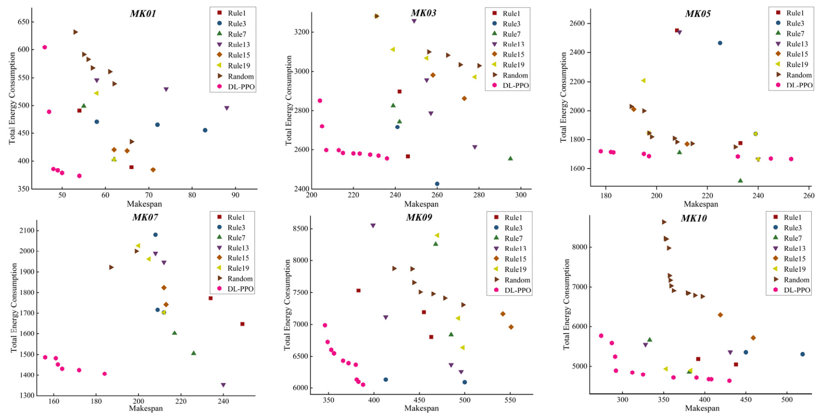
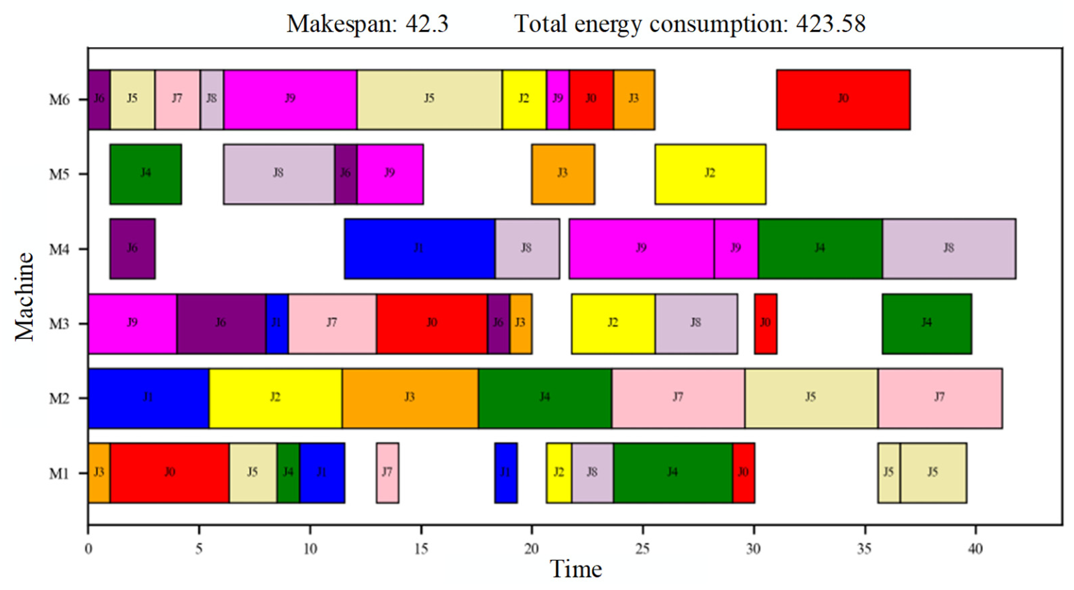
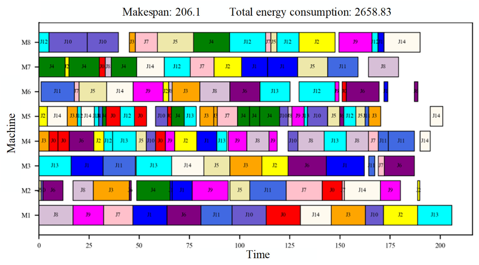
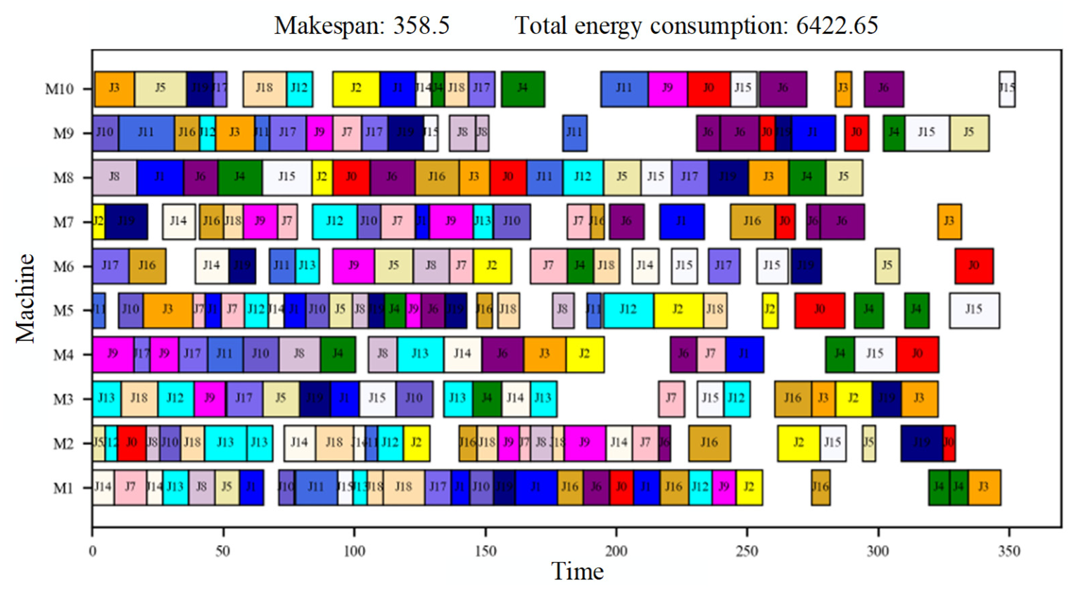
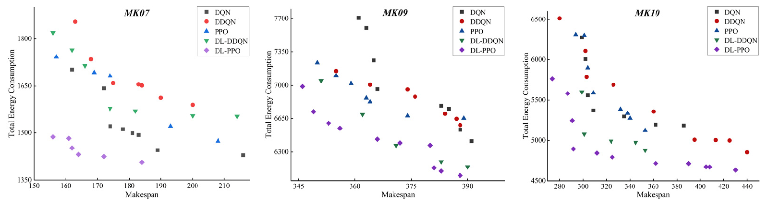
Figure 5 and Figure 6 further illustrate that DL-PPO achieves better trade-offs between makespan and energy consumption across different benchmark instances. As the problem scale increases, the superiority of DL-PPO becomes more evident, and it consistently generates more competitive and well-distributed Pareto fronts under larger-scale scheduling scenarios. Moreover, Figure 7, Figure 8 and Figure 9 present the Gantt charts of the scheduling results obtained by the proposed method under different problem scales. These figures provide a clear and intuitive visualization of operation sequences and machine assignments, further demonstrating the effectiveness and practical applicability of the proposed scheduling strategy.

5.4. Comparisons with Deep Reinforcement Learning Methods

To further verify the effectiveness of DL-PPO, it is compared with three other DRL methods, including DQN, DDQN, and PPO. In addition, to evaluate the training efficiency of the algorithm, a comparison is made with the Dual-Layer Double Deep Q-Network (DL-DDQN) algorithm under the condition that other experimental settings remain identical. Specifically, both the high-level and low-level controllers in DL-DDQN are implemented based on the DDQN algorithm. To ensure fairness, all methods employ the same dual-decision-point dispatching rules. Each method is run 10 times independently on each benchmark instance. The $C_{\max }^{ave}$, $T{E}^{ave}$, GD, IGD and $\Delta$ obtained from different methods on each benchmark instance are calculated and compared. The comparative results are shown in Table 10,

Table 11. $T{E}^{ave}$ obtained by DL-PPO and other DRL methods.

Benchmark Instance	Scale	DQN	DDQN	PPO	DL-DDQN	DL-PPO
		$\mathit{T}{\mathit{E}}^{\mathit{a}\mathit{v}\mathit{e}}$	$\mathit{T}{\mathit{E}}^{\mathit{a}\mathit{v}\mathit{e}}$	$\mathit{T}{\mathit{E}}^{\mathit{a}\mathit{v}\mathit{e}}$	$\mathit{T}{\mathit{E}}^{\mathit{a}\mathit{v}\mathit{e}}$	$\mathit{T}{\mathit{E}}^{\mathit{a}\mathit{v}\mathit{e}}$
MK01	10 $\times$ 6	420.82	422.63	425.19	419.29	418.78
MK02	10 $\times$ 6	395.19	380.37	409.42	378.55	373.85
MK03	15 $\times$ 8	2873.68	2840.71	2725.29	2675.20	2614.43
MK04	15 $\times$ 8	1051.73	1045.62	1079.24	989.37	974.90
MK05	15 $\times$ 4	2078.28	1824.34	1953.76	1580.03	1862.90
MK06	10 $\times$ 15	1145.34	1123.61	1087.35	1022.48	1065.26
MK07	20 $\times$ 5	1602.37	1702.46	1622.39	1578.71	1563.62
MK08	20 $\times$ 10	8182.87	8381.29	8375.21	8124.80	7949.73
MK09	20 $\times$ 10	6802.43	6701.22	6582.64	6433.17	6380.76
MK10	20 $\times$ 15	5298.23	5399.12	5385.90	5136.74	5103.36

,

Table 12. GD for the Pareto-optimal fronts obtained by DL-PPO and other DRL methods.

Benchmark Instance	Scale	DQN	DDQN	PPO	DL-DDQN	DL-PPO
		GD	GD	GD	GD	GD
MK01	10 $\times$ 6	0.429	0.961	1.263	0.558	0.493
MK02	10 $\times$ 6	0.523	0.143	0.698	0.429	0.101
MK03	15 $\times$ 8	1.199	0.580	0.725	0.206	0.009
MK04	15 $\times$ 8	1.453	0.321	0.933	1.171	0.163
MK05	15 $\times$ 4	0.556	0.245	0.347	0.100	0.298
MK06	10 $\times$ 15	0.335	0.140	0.281	0.103	0.039
MK07	20 $\times$ 5	1.381	2.778	2.297	2.626	0.000
MK08	20 $\times$ 10	0.811	3.131	1.734	1.686	0.550
MK09	20 $\times$ 10	0.583	0.472	0.353	0.128	0.068
MK10	20 $\times$ 15	0.333	0.360	0.349	0.156	0.000

,

Table 13. IGD for the Pareto-optimal fronts obtained by DL-PPO and other DRL methods.

Benchmark Instance	Scale	DQN	DDQN	PPO	DL-DDQN	DL-PPO
		IGD	IGD	IGD	IGD	IGD
MK01	10 $\times$ 6	0.407	0.685	0.670	0.250	0.149
MK02	10 $\times$ 6	0.372	0.378	0.534	0.185	0.070
MK03	15 $\times$ 8	1.330	0.776	0.435	0.171	0.052
MK04	15 $\times$ 8	0.397	0.548	0.931	0.378	0.072
MK05	15 $\times$ 4	0.636	0.173	0.422	0.109	0.253
MK06	10 $\times$ 15	0.325	0.124	0.332	0.190	0.039
MK07	20 $\times$ 5	0.749	2.189	1.362	1.666	0.000
MK08	20 $\times$ 10	0.673	0.503	0.956	0.234	0.261
MK09	20 $\times$ 10	0.457	0.490	0.446	0.171	0.011
MK10	20 $\times$ 15	0.400	0.375	0.414	0.279	0.000

and

Table 14. $\Delta$ values for the Pareto-optimal fronts obtained by DL-PPO and other DRL methods.

Benchmark Instance	Scale	DQN	DDQN	PPO	DL-DDQN	DL-PPO
		$\Delta$	$\Delta$	$\Delta$	$\Delta$	$\Delta$
MK01	10 $\times$ 6	0.638	0.648	0.739	0.861	0.832
MK02	10 $\times$ 6	0.674	0.700	0.786	0.812	0.664
MK03	15 $\times$ 8	0.805	0.653	0.754	0.743	0.547
MK04	15 $\times$ 8	0.910	1.034	0.858	1.051	0.751
MK05	15 $\times$ 4	0.869	0.850	0.781	0.722	0.888
MK06	10 $\times$ 15	0.813	0.848	0.654	0.687	0.693
MK07	20 $\times$ 5	0.842	0.873	0.835	0.773	0.691
MK08	20 $\times$ 10	0.784	1.138	0.794	0.919	0.780
MK09	20 $\times$ 10	0.747	0.789	0.754	0.596	0.562
MK10	20 $\times$ 15	0.756	0.794	0.868	0.870	0.749

.

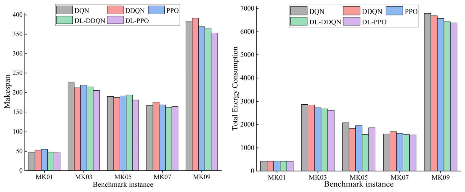
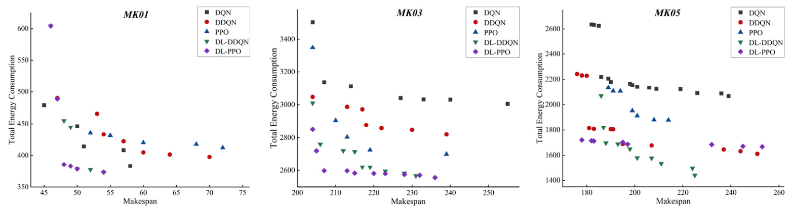
From the experimental results reported in Table 10, Table 11, Table 12, Table 13 and Table 14, it can be observed that DL-PPO achieves the best or near-best performance in most benchmark instances in terms of makespan and energy consumption. Compared with DQN, DDQN, and PPO, DL-PPO consistently reduces both objective values, indicating that the hierarchical policy learning mechanism can more effectively coordinate scheduling decisions under energy-aware constraints. Compared with DL-DDQN, DL-PPO still shows overall improvement, which demonstrates the advantage of policy-gradient-based optimization in learning more stable scheduling strategies. For convergence-related indicators, DL-PPO generally obtains the lowest GD and IGD values across most instances, indicating that the obtained solutions are closer to the true Pareto front and exhibit better convergence performance. In several cases, DL-PPO achieves the best results among all compared methods, further confirming its effectiveness in multi-objective optimization. In addition, the Spread results show that DL-PPO maintains good performance in most instances, indicating a reasonable balance between the convergence and diversity of the obtained Pareto solutions. Figure 10 compares the average values of two objectives obtained by DL-PPO and other DRL methods across benchmark instances of different scales. Figure 11 compares the Pareto frontiers obtained by DL-PPO and other DRL methods for the same instances.

To further verify the performance of the proposed algorithm, comparative experiments on training time and convergence episodes of different algorithms are conducted using benchmark instances.

Table 15. Training time and gap comparison of different algorithms on benchmark instances.

Benchmark Instance	Scale	Training Time (min)
		DQN		DDQN		PPO		DL-DDQN		DL-PPO
		Time	Gap	Time	Gap	Time	Gap	Time	Gap	Time	Gap
MK01	10 $\times$ 6	4.85	0.00%	5.10	5.15%	5.32	9.69%	5.39	11.13%	5.45	12.37%
MK02	10 $\times$ 6	5.01	1.21%	5.12	3.43%	4.95	0.00%	6.29	27.07%	6.07	22.63%
MK03	15 $\times$ 8	33.25	0.27%	34.71	4.67%	33.16	0.00%	36.93	11.37%	36.80	10.98%
MK04	15 $\times$ 8	7.97	0.00%	8.23	3.26%	8.15	2.26%	10.65	33.63%	9.46	18.70%
MK05	15 $\times$ 4	11.04	9.52%	11.19	11.01%	10.08	0.00%	15.11	49.90%	14.33	42.16%
MK06	10 $\times$ 15	45.12	2.43%	45.50	3.29%	44.05	0.00%	47.13	6.99%	46.66	5.93%
MK07	20 $\times$ 5	14.11	0.00%	15.22	7.87%	14.71	4.25%	16.35	15.88%	17.07	20.98%
MK08	20 $\times$ 10	30.15	1.79%	31.46	6.21%	29.62	0.00%	36.37	22.79%	35.44	19.65%
MK09	20 $\times$ 10	36.06	0.59%	36.33	1.34%	35.85	0.00%	41.12	14.70%	40.41	12.72%
MK10	20 $\times$ 15	32.57	3.63%	33.86	7.73%	31.43	0.00%	37.69	19.92%	36.32	15.56%

shows the overall training time of the proposed DL-PPO algorithm. DL-PPO has longer training time than DQN, DDQN, PPO and DL-DDQN, with its time gap rising slightly. This result stems from DL-PPO’s hierarchical reinforcement learning structure. Its dual decision-making framework and multi-dimensional state feature extraction raise computational consumption in model propagation and parameter optimization, increasing total training time. The gap values verify the rational time difference between DL-PPO and comparison algorithms, with no serious efficiency loss.

Table 16. Comparison of convergence episodes among different algorithms.

Benchmark Instance	Scale	DQN	DDQN	PPO	DL-DDQN	DL-PPO
		Convergence Episodes	Convergence Episodes	Convergence Episodes	Convergence Episodes	Convergence Episodes
MK01	10 $\times$ 6	1500	1600	210	1580	100
MK02	10 $\times$ 6	1620	1550	180	1300	120
MK03	15 $\times$ 8	1550	1700	240	1250	140
MK04	15 $\times$ 8	1780	1650	220	1400	110
MK05	15 $\times$ 4	1680	1820	260	1350	160
MK06	10 $\times$ 15	1900	1750	300	1600	130
MK07	20 $\times$ 5	1820	1880	280	1550	200
MK08	20 $\times$ 10	2050	1920	350	1700	200
MK09	20 $\times$ 10	2150	2050	420	1800	260
MK10	20 $\times$ 15	2250	2180	480	1950	240

presents the convergence episodes of all algorithms. DL-PPO obtains the minimum convergence episodes in all test instances and shows better convergence efficiency than other comparison methods. The hierarchical reinforcement learning structure brings extra computational cost, leading to no advantage in total training time, but effectively optimizes the policy update process, reduces model convergence iteration steps, and cuts numerous invalid iterative operations. DL-PPO sacrifices acceptable training time cost to achieve high convergence performance and stable solution ability. The proposed DL-PPO method has superior comprehensive performance in solving energy-aware flexible job shop scheduling problems.

5.5. Engineering Case Validation

The engineering case in this section comes from the welding workshop of a Tunnel Boring Machine cutterhead manufacturing enterprise. This workshop is used to complete welding and forming tasks of key cutterhead structures. Specifically, the workshop includes 17 machines. These machines cover welding, heat treatment, and machining processes. The equipment includes two gas-shielded welding machines, two submerged arc welding machines, three repair welding stations, two surfacing welding stations, and one riveting welding station. It also includes auxiliary machines. These machines include two CNC milling machines, two heating furnaces, one quenching furnace, one grinding station, and one cooling station.

Some welding operations of the TBM cutterhead can be processed by multiple alternative machines. These machines meet the same processing requirements. Therefore, machine assignment has high flexibility and uncertainty. This feature increases the complexity of scheduling decisions in the workshop. It also makes the problem suitable for modeling as a Markov decision process and solving by deep reinforcement learning. This section uses real production data from the TBM cutterhead welding workshop. It constructs an engineering case with three typical cutterhead types. These types include the center cutterhead, the assembled cutterhead, and the integral cutterhead. The process routes and related information are shown in

Table 17. Process routes and related parameters of different types of TBM cutterheads.

Cutterhead Type	Welding Operation	Processing Machine		Processing Time
Integral cutterhead	Tack welding of cutterhead	Gas-shielded welding machine	M2	3
			M3	3
	Structural welding of cutterhead	Submerged arc welding machine	M8	7
			M9	7
	Weld seam filling of cutterhead	Repair welding station	M12	5
			M13	5
			M14	5
	Annealing treatment	Heating furnace	M10	4
			M11	4
	Transition layer surfacing	Surfacing welding station	M6	5
			M7	5
	Wear-resistant layer surfacing	Surfacing welding station	M6	6
			M7	6
	CNC milling	CNC milling machine	M4	3
			M5	3
	Quenching treatment	Quenching furnace	M15	2
	Tempering treatment	Heating furnace	M10	4
			M11	4
Assembled cutterhead	Grinding and inspection	Grinding station	M1	2
	Transition layer surfacing	Surfacing welding station	M6	5
			M7	5
	CNC milling	CNC milling machine	M4	4
			M5	4
	Riveting and welding of cutterhead assembly	Riveting welding station	M16	3
	Preheating treatment	Heating furnace	M10	2
			M11	2
	Weld seam filling of cutterhead assembly	Repair welding station	M12	6
			M13	6
			M14	6
	Annealing treatment	Heating furnace	M10	3
			M11	3
	Quenching treatment	Quenching furnace	M15	1
	Tempering treatment	Heating furnace	M10	4
			M11	4
	Cooling treatment	Cooling station	M17	8
Center cutterhead	Transition layer surfacing	Surfacing welding station	M6	6
			M7	6
	Annealing treatment	Heating furnace	M10	3
			M11	3
	Riveting and welding of cutter seat and support plate	Riveting welding station	M16	4
	Weld seam filling of center cutterhead	Repair welding station	M12	7
			M13	7
			M14	7
	Annealing treatment	Heating furnace	M10	4
			M11	4
	CNC milling	CNC milling machine	M4	6
			M5	6
	Quenching treatment	Quenching furnace	M15	2
	Tempering treatment	Heating furnace	M10	4
			M11	4

. The processing time of each welding operation on different machines is obtained from actual production data.

The power parameters of all machines are defined based on actual operating data from the workshop. The setup ignores the energy consumption caused by machine start-up and preheating. Each machine has two states. These states include the processing state and the idle state. The power values for these states are specified according to real production conditions. The related parameters are listed in

Table 18. Power parameters of equipment energy consumption in the TBM cutterhead welding workshop.

Machine	Equipment Power
	Processing Power	Idle Power
Gas-shielded welding machine	1.5	0.13
Submerged arc welding machine	1.5	0.13
Repair welding station	1.8	0.25
Surfacing welding station	1.7	0.20
Riveting welding station	1.6	0.15
Grinding station	0.7	0.10
CNC milling machine	0.6	0.10
Heating furnace	2.0	0.30
Quenching furnace	1.8	0.15
Cooling station	0.5	0.10

.

This study evaluates the performance of DL-PPO under different production scales. It builds multiple practical scheduling scenarios based on real workshop conditions. The total number of cutterheads is set to 10, 15, 20, 25, 30, 35, 40, 45, and 50. These scenarios cover small-batch and large-batch production. They reflect different levels of scheduling complexity. The current scheduling in the TBM cutterhead welding workshop relies on manual experience. This study collects and simulates scheduling data under the given production scales. The results of manual scheduling are reported in

Table 19. Comparison of makespan results of different methods under different production scales.

Production Scale	Current Workshop		DQN		DDQN		PPO		DL-DDQN		DL-PPO
	${\mathit{C}}_{\mathbf{max}}^{\mathit{a}\mathit{v}\mathit{e}}$	Gap	${\mathit{C}}_{\mathbf{max}}^{\mathit{a}\mathit{v}\mathit{e}}$	Gap	${\mathit{C}}_{\mathbf{max}}^{\mathit{a}\mathit{v}\mathit{e}}$	Gap	${\mathit{C}}_{\mathbf{max}}^{\mathit{a}\mathit{v}\mathit{e}}$	Gap	${\mathit{C}}_{\mathbf{max}}^{\mathit{a}\mathit{v}\mathit{e}}$	Gap	${\mathit{C}}_{\mathbf{max}}^{\mathit{a}\mathit{v}\mathit{e}}$	Gap
10 $\times$ 17	92.04	42.43%	69.32	7.27%	70.70	9.41%	66.67	3.17%	66.44	2.82%	64.62	0.00%
15 $\times$ 17	140.30	56.55%	92.85	3.60%	89.62	0.00%	93.41	4.23%	90.86	1.38%	90.57	1.06%
20 $\times$ 17	186.57	62.48%	115.57	0.64%	116.20	1.19%	115.13	0.26%	119.10	3.72%	114.83	0.00%
25 $\times$ 17	230.84	63.38%	157.28	11.32%	143.36	1.47%	149.48	5.80%	153.94	8.95%	141.29	0.00%
30 $\times$ 17	270.41	63.09%	167.89	1.26%	167.61	1.09%	177.64	7.14%	170.08	2.58%	165.80	0.00%
35 $\times$ 17	312.85	66.32%	192.30	2.23%	189.75	0.88%	201.62	7.19%	194.88	3.60%	188.10	0.00%
40 $\times$ 17	355.40	68.72%	215.90	2.49%	212.40	0.83%	228.35	8.40%	219.70	4.30%	210.65	0.00%
45 $\times$ 17	398.60	89.22%	238.75	13.34%	235.20	11.65%	252.90	20.06%	243.15	15.43%	210.65	0.00%
50 $\times$ 17	442.30	72.64%	262.10	2.30%	258.55	0.92%	277.80	8.43%	266.90	4.18%	256.20	0.00%

and

Table 20. Comparison of total energy consumption results of different methods under different production scales.

Production Scale	Current Workshop		DQN		DDQN		PPO		DL-DDQN		DL-PPO
	$\mathit{T}{\mathit{E}}^{\mathit{a}\mathit{v}\mathit{e}}$	Gap	$\mathit{T}{\mathit{E}}^{\mathit{a}\mathit{v}\mathit{e}}$	Gap	$\mathit{T}{\mathit{E}}^{\mathit{a}\mathit{v}\mathit{e}}$	Gap	$\mathit{T}{\mathit{E}}^{\mathit{a}\mathit{v}\mathit{e}}$	Gap	$\mathit{T}{\mathit{E}}^{\mathit{a}\mathit{v}\mathit{e}}$	Gap	$\mathit{T}{\mathit{E}}^{\mathit{a}\mathit{v}\mathit{e}}$	Gap
10 $\times$ 17	514.46	6.37%	505.38	4.49%	493.03	1.94%	497.67	2.90%	495.58	2.46%	483.66	0.00%
15 $\times$ 17	756.71	6.18%	738.56	3.64%	732.73	2.82%	740.67	3.93%	712.65	0.00%	716.10	0.48%
20 $\times$ 17	1012.17	7.43%	942.50	0.03%	972.26	3.19%	942.18	0.00%	955.05	1.37%	945.03	0.30%
25 $\times$ 17	1260.92	7.93%	1230.60	5.33%	1203.88	3.04%	1215.52	4.04%	1191.73	2.00%	1168.32	0.00%
30 $\times$ 17	1490.04	7.00%	1423.97	2.26%	1428.16	2.56%	1395.63	0.22%	1403.63	0.80%	1392.55	0.00%
35 $\times$ 17	1728.60	6.81%	1658.75	2.50%	1665.20	2.89%	1628.40	0.62%	1635.10	1.04%	1618.35	0.00%
40 $\times$ 17	1965.80	7.10%	1885.90	2.74%	1892.75	3.12%	1848.60	0.71%	1856.20	1.13%	1835.55	0.00%
45 $\times$ 17	2205.40	7.02%	2115.30	2.64%	2122.10	2.97%	2078.45	0.86%	2086.70	1.26%	2060.80	0.00%
50 $\times$ 17	2448.20	17.79%	2348.60	13.00%	2355.25	13.32%	2078.45	0.00%	2316.40	11.45%	2285.75	9.97%

. These results are listed as “Current workshop”. The evaluation considers the makespan and total energy consumption. This study further evaluates DL-PPO in the same instances. It compares MAHRL-CS with DQN, DDQN, PPO, and DL-DDQN. Each method runs 10 independent trials for each production scale. Each trial records makespan and total energy consumption. The minimum value of each metric is selected in each trial. The study then computes the average of these minimum values over 10 trials. This process evaluates the overall scheduling performance of each method. The comparison results are shown in Table 20.

The results show clear improvements over manual scheduling. The manual policy is based on human experience. DRL methods achieve lower makespan and lower total energy consumption. This result indicates that DRL can learn scheduling policies in complex environments. It enables end-to-end optimization of job sequencing and machine assignment. The study also compares different DRL methods. DL-PPO achieves balanced performance across all production scales. It reduces the makespan and total energy consumption at the same time. This result improves overall scheduling performance. It confirms the feasibility of DL-PPO in the TBM cutterhead welding workshop. It also shows its practical value in real scheduling applications.

6. Conclusions and Future Work

In this paper, a Dual-Layer Proximal Policy Optimization algorithm (DL-PPO) is proposed for the Energy-Aware Flexible Job Shop Scheduling Problem (EA-FJSP), aiming at the collaborative optimization of makespan and total energy consumption. Based on the proposed DL-PPO, a hierarchical scheduling framework is designed, which includes a high-level controller and a low-level controller. At each scheduling point, the high-level controller determines the temporary optimization direction by selecting the sub-objective decomposed from the global optimization objective, while the low-level controller selects a feasible dispatching rule according to the temporary optimization direction. A multi-dimensional state representation of the scheduling environment is achieved by extracting twelve state features covering four dimensions: job, machine, time, and energy consumption. In response to the characteristics of the EA-FJSP, twenty dual-decision-point dispatching rules are designed as the action space for the low-level controller, thereby enhancing the scheduling flexibility and adaptability of the algorithm. To achieve multi-objective collaborative optimization, four targeted reward functions are designed based on sub-objectives. Each reward function aims to optimize either the makespan or the total energy consumption. In the experimental validation, five performance evaluation metrics are employed to conduct a comparative analysis of DL-PPO against dispatching rules and other DRL methods. The results demonstrate the superior capability of DL-PPO, validating its applicability and effectiveness in solving the EA-FJSP.

Although the proposed DL-PPO demonstrates strong performance in solving the EA-FJSP, several limitations still exist. First, the current model relies on manually designed state features and dispatching rules, which may limit its ability to capture more complex structural relationships in the scheduling environment. Second, the framework primarily focuses on static scheduling scenarios, and its adaptability to dynamic and uncertain environments requires further investigation. In addition, the integration of advanced learning paradigms for improving generalization ability and global optimization performance has not been fully explored. Future research work can focus on the following aspects:

• By abstracting the scheduling environment into a graph structure and integrating graph neural networks with other graph representation learning techniques, the complex relationships between jobs and machines can be captured from a graph perspective, enhancing the capability of the model to characterize the scheduling environment.
• Integrating deep reinforcement learning with emerging AI techniques such as evolutionary algorithms, self-supervised learning, and meta-learning to enhance the ability to address multi-objective trade-offs in energy-aware scheduling while improving the generalization and global optimization capabilities of scheduling policies.
• Expanding to the EA-FJSP in dynamic environments, combining event-driven mechanisms with real-time decision-making models, enhancing the adaptability of the method and its practicality in dynamic and uncertain environments.

References

1. Destouet, C.; Tlahig, H.; Bettayeb, B.; Mazari, B. Flexible job shop scheduling problem under Industry 5.0: A survey on human reintegration, environmental consideration and resilience improvement. J. Manuf. Syst. 2023, 67, 155–173. [Google Scholar] [CrossRef]
2. Dauzère-Pérès, S.; Ding, J.; Shen, L.; Tamssaouet, K. The flexible job shop scheduling problem: A review. Eur. J. Oper. Res. 2023, 314, 409–432. [Google Scholar] [CrossRef]
3. Li, M.; Wang, G.G. A review of green shop scheduling problem. Inf. Sci. 2021, 589, 478–496. [Google Scholar] [CrossRef]
4. Fekih, A.; Hajji, M.K. Optimizing logistics and production flows for sustainability in green flexible job-shops. Acta Logist. 2026, 13, 114–126. [Google Scholar] [CrossRef]
5. Jarboui, B.; Eddaly, M. A branch-and-bound approach to the no-idle flowshop scheduling problem. Discret. Appl. Math. 2024, 347, 297–310. [Google Scholar] [CrossRef]
6. Türkyılmaz, A.; Şenvar, Ö.; Ünal, I.; Bulkan, S. A research survey: Heuristic approaches for solving multi objective flexible job shop problems. J. Intell. Manuf. 2020, 31, 1949–1983. [Google Scholar] [CrossRef]
7. Zhang, W.; Luo, Z.; Zhang, S. Production-logistics cooperative scheduling in a two-stage assembly flow-shop with deteriorating robotic arm: A problem-specific heuristic. Comput. Oper. Res. 2026, 189, 107409. [Google Scholar] [CrossRef]
8. Wang, Y.-J.; Wang, G.-G.; Tian, F.-M.; Gong, D.-W.; Pedrycz, W. Solving energy-efficient fuzzy hybrid flow-shop scheduling problem at a variable machine speed using an extended NSGA-II. Eng. Appl. Artif. Intell. 2023, 121, 105977. [Google Scholar] [CrossRef]
9. Li, X.; Wu, C.; Wu, R.; Tang, H. Multi-objective fuzzy green scheduling optimization method of special vehicle body-in-white prototype shop considering equipment preventive maintenance. J. Clean. Prod. 2024, 462, 142660. [Google Scholar] [CrossRef]
10. Wang, J.; Lei, D.; Tang, H. A multi-objective dynamical artificial bee colony for energy-efficient fuzzy hybrid flow shop scheduling with batch processing machines. Expert Syst. Appl. 2025, 259, 125244. [Google Scholar] [CrossRef]
11. Han, B.A.; Yang, J.J. Research on adaptive job shop scheduling problems based on dueling double DQN. IEEE Access 2020, 8, 186474–186495. [Google Scholar] [CrossRef]
12. Yuan, E.; Wang, L.; Cheng, S.; Song, S.; Fan, W.; Li, Y. Solving flexible job shop scheduling problems via deep reinforcement learning. Expert Syst. Appl. 2024, 245, 123019. [Google Scholar] [CrossRef]
13. Song, W.; Chen, X.; Li, Q.; Cao, Z. Flexible job-shop scheduling via graph neural network and deep reinforcement learning. IEEE Trans. Ind. Inform. 2022, 19, 1600–1610. [Google Scholar] [CrossRef]
14. Pernas-Álvarez, J.; Becerra, J.A.; Crespo-Pereira, D. Comparison of exact methods and metaheuristics to solve the flexible Job-Shop assembly problem in frigate shipbuilding. Ships Offshore Struct. 2026, 1–24. [Google Scholar] [CrossRef]
15. Wu, X.; Yan, X.; Guan, D.; Wei, M. A deep reinforcement learning model for dynamic job-shop scheduling problem with uncertain processing time. Eng. Appl. Artif. Intell. 2024, 131, 107790. [Google Scholar] [CrossRef]
16. Zhang, W.; Zhao, F.; Li, Y.; Du, C.; Feng, X.; Mei, X. A novel collaborative agent reinforcement learning framework based on an attention mechanism and disjunctive graph embedding for flexible job shop scheduling problem. J. Manuf. Syst. 2024, 74, 329–345, Correction in J. Manuf. Syst. 2024, 75, 333. https://doi.org/10.1016/j.jmsy.2024.04.009. [Google Scholar] [CrossRef]
17. Le, N.; Rathour, V.S.; Yamazaki, K.; Luu, K.; Savvides, M. Deep reinforcement learning in computer vision: A comprehensive survey. Artif. Intell. Rev. 2022, 55, 2733–2819. [Google Scholar] [CrossRef]
18. Hickling, T.; Zenati, A.; Aouf, N.; Spencer, P. Explain ability in deep reinforcement learning: A review into current methods and applications. ACM Comput. Surv. 2023, 56, 1–35. [Google Scholar] [CrossRef]
19. Li, Y.; Tao, Z.; Wang, L.; Du, B.; Guo, J.; Pang, S. Digital twin-based job shop anomaly detection and dynamic scheduling. Robot. Comput.-Integr. Manuf. 2023, 79, 102443. [Google Scholar] [CrossRef]
20. Luo, S.; Zhang, L.; Fan, Y. Real-time scheduling for dynamic partial-no-wait multi objective flexible job shop by deep reinforcement learning. IEEE Trans. Autom. Sci. Eng. 2021, 19, 3020–3038. [Google Scholar] [CrossRef]
21. Hou, Z.; Fei, J.; Deng, Y.; Xu, J. Data-efficient hierarchical reinforcement learning for robotic assembly control applications. IEEE Trans. Ind. Electron. 2020, 68, 11565–11575. [Google Scholar] [CrossRef]
22. Li, J.; Li, H.; He, P.; Xu, L.; He, K.; Liu, S. Flexible job shop scheduling optimization for green manufacturing based on improved multi-objective wolf pack algorithm. Appl. Sci. 2023, 13, 8535. [Google Scholar] [CrossRef]
23. Wei, S.; Tang, H.; Li, X.; Lei, D.; Wang, X.V. An improved memetic algorithm for multi-objective resource-constrained flexible job shop inverse scheduling problem: An application for machining workshop. J. Manuf. Syst. 2024, 74, 264–290. [Google Scholar] [CrossRef]
24. Gong, G.; Tang, J.; Huang, D.; Luo, Q.; Zhu, K.; Peng, N. Energy-efficient flexible job shop scheduling problem considering discrete operation sequence flexibility. Swarm Evol. Comput. 2024, 84, 101421. [Google Scholar] [CrossRef]
25. Xu, S.; Li, Y.; Li, Q. A deep reinforcement learning method based on a transformer model for the flexible job shop scheduling problem. Electronics 2024, 13, 3696. [Google Scholar] [CrossRef]
26. Peng, Z.; Zhang, H.; Tang, H.; Feng, Y.; Yin, W. Research on flexible job-shop scheduling problem in green sustainable manufacturing based on learning effect. J. Intell. Manuf. 2022, 33, 1725–1746. [Google Scholar] [CrossRef]
27. Li, J.; Guo, X.; Yang, Y.; Zhang, Q. A hybrid algorithm for multi-objective optimization-combining a biogeography-based optimization and symbiotic organisms search. Symmetry 2023, 15, 1481. [Google Scholar] [CrossRef]
28. Hu, Y.; Zhang, L.; Wang, Q.; Zhang, Z.; Tang, Q. A matheuristic-based multi-objective evolutionary algorithm for flexible assembly jobs shop scheduling problem in cellular manufacture. Swarm Evol. Comput. 2024, 87, 101549. [Google Scholar] [CrossRef]
29. Huang, J.-P.; Gao, L.; Li, X.-Y.; Zhang, C.-J. A novel priority dispatch rule generation method based on graph neural network and reinforcement learning for distributed job-shop scheduling. J. Manuf. Syst. 2023, 69, 119–134. [Google Scholar] [CrossRef]
30. Zhang, K.; Bi, L.; Jiao, X. Research on flexible job-shop scheduling problems with integrated reinforcement learning algorithm. China Mech. Eng. 2023, 34, 201–207. [Google Scholar] [CrossRef]
31. Gong, H.; Xu, W.; Sun, W.; Xu, K. Multi-Objective Flexible Flow Shop Production Scheduling Problem Based on the Double Deep Q-Network Algorithm. Processes 2023, 11, 3321. [Google Scholar] [CrossRef]
32. Yao, Y.; Li, X.; Gao, L. A DQN-based memetic algorithm for energy-efficient job shop scheduling problem with integrated limited AGVs. Swarm Evol. Comput. 2024, 87, 101544. [Google Scholar] [CrossRef]
33. Liang, P.; Xiao, P.; Li, Z.; Luo, M.; Zhang, C. A novel deep reinforcement learning-based algorithm for multi-objective energy-efficient flow-shop scheduling. IET Collab. Intell. Manuf. 2024, 6, e12121. [Google Scholar] [CrossRef]
34. Wang, S.; Li, J.; Tang, H.; Wang, J. CEA-FJSP: Carbon emission-aware flexible job-shop scheduling based on deep reinforcement learning. Front. Environ. Sci. 2022, 10, 1059451. [Google Scholar] [CrossRef]
35. Tang, Y.; Shen, L.; Han, S. Low-Carbon Flexible Job Shop Scheduling Problem Based on Deep Reinforcement Learning. Sustainability 2024, 16, 4544. [Google Scholar] [CrossRef]
36. Lu, Y.; Yuan, Y.; Sitahong, A.; Chao, Y.; Wang, Y. An Optimization Method for Green Permutation Flow Shop Scheduling Based on Deep Reinforcement Learning and MOEA/D. Machines 2024, 12, 721. [Google Scholar] [CrossRef]
37. Gronauer, S.; Diepold, K. Multi-agent deep reinforcement learning: A survey. Artif. Intell. Rev. 2022, 55, 895–943. [Google Scholar] [CrossRef]
38. Yuan, M.; Huang, H.; Li, Z.; Zhang, C.; Pei, F.; Gu, W. A multi-agent double deep-Q-network based on state machine and event stream for flexible job shop scheduling problem. Adv. Eng. Inform. 2023, 58, 102230. [Google Scholar] [CrossRef]
39. Liu, R.; Piplani, R.; Toro, C. A deep multi-agent reinforcement learning approach to solve dynamic job shop scheduling problem. Comput. Oper. Res. 2023, 159, 106294. [Google Scholar] [CrossRef]
40. Wu, J.; Liu, Y. A modified multi-agent proximal policy optimization algorithm for multi-objective dynamic partial-re-entrant hybrid flow shop scheduling problem. Eng. Appl. Artif. Intell. 2025, 140, 109688. [Google Scholar] [CrossRef]
41. Qiu, J.; Liu, J.; Li, Z.; Lai, X. A multi-level action coupling reinforcement learning approach for online two-stage flexible assembly flow shop scheduling. J. Manuf. Syst. 2024, 76, 351–370. [Google Scholar] [CrossRef]
42. Gui, Y.; Tang, D.; Zhu, H.; Zhang, Y.; Zhang, Z. Dynamic scheduling for flexible job shop using a deep reinforcement learning approach. Comput. Ind. Eng. 2023, 180, 109255. [Google Scholar] [CrossRef]
43. Ding, L.; Guan, Z.; Rauf, M.; Yue, L. Multi-policy deep reinforcement learning for multi-objective multiplicity flexible job shop scheduling. Swarm Evol. Comput. 2023, 87, 101550. [Google Scholar] [CrossRef]
44. Wang, R.; Wang, G.; Sun, J.; Deng, F.; Chen, J. Flexible job shop scheduling via dual attention network-based reinforcement learning. IEEE Trans. Neural Netw. Learn. Syst. 2023, 35, 3091–3102. [Google Scholar] [CrossRef]
45. Lei, K.; Guo, P.; Zhao, W.; Wang, Y.; Qian, L.; Meng, X.; Tang, L. A multi-action deep reinforcement learning framework for flexible Job-shop scheduling problem. Expert Syst. Appl. 2022, 205, 117796. [Google Scholar] [CrossRef]
46. Wan, L.; Fu, L.; Li, C.; Li, K. Flexible job shop scheduling via deep reinforcement learning with meta-path-based heterogeneous graph neural network. Knowl.-Based Syst. 2024, 296, 111940. [Google Scholar] [CrossRef]
47. Wang, M.; Zhang, J.; Zhang, P.; Cui, L.; Zhang, G. Independent double DQN-based multi-agent reinforcement learning approach for online two-stage hybrid flow shop scheduling with batch machines. J. Manuf. Syst. 2022, 65, 694–708. [Google Scholar] [CrossRef]
48. Lu, S.; Wang, Y.; Kong, M.; Wang, W.; Tan, W.; Song, Y. A Double Deep Q-Network framework for a flexible job shop scheduling problem with dynamic job arrivals and urgent job insertions. Eng. Appl. Artif. Intell. 2024, 133, 108487. [Google Scholar] [CrossRef]
49. Tang, Y.; Guo, S.; Liu, J.; Wan, B.; An, L.; Liu, J.K. Hierarchical reinforcement learning from imperfect demonstrations through reachable coverage-based subgoal filtering. Knowl.-Based Syst. 2024, 294, 111736. [Google Scholar] [CrossRef]
50. Wang, Q.; Lai, K.H.; Tang, C. Solving combinatorial optimization problems over graphs with BERT-Based Deep Reinforcement Learning. Inf. Sci. 2023, 619, 930–946. [Google Scholar] [CrossRef]
51. Li, Y.; Guan, Q.; Gu, J.F.; Jiang, X.; Li, Y. A hierarchical deep reinforcement learning method for solving urban route planning problems under large-scale customers and real-time traffic conditions. Int. J. Geogr. Inf. Sci. 2025, 39, 118–141. [Google Scholar] [CrossRef]
52. Liu, J.F.; Wang, Z.H.; Zhang, W.; Zhang, C.R.; Hou, J.F.; Bai, B.; Zhang, G. HiTSP: Towards a Hierarchical Neural Framework for Large-scale Traveling Salesman Problems. J. Oper. Res. Soc. China 2023, 13, 1083–1107. [Google Scholar] [CrossRef]
53. Si, J.; He, F.; Lin, X.; Tang, X. Vehicle dispatching and routing of on-demand intercity ride-pooling services: A multi-agent hierarchical reinforcement learning approach. Transp. Res. Part E Logist. Transp. Rev. 2024, 186, 103551. [Google Scholar] [CrossRef]
54. Wang, J.; Gao, P.; Zheng, P.; Zhang, J.; Ip, W. A fuzzy hierarchical reinforcement learning based scheduling method for semiconductor wafer manufacturing systems. J. Manuf. Syst. 2021, 61, 239–248. [Google Scholar] [CrossRef]
55. Luo, S.; Zhang, L.; Fan, Y. Dynamic multi-objective scheduling for flexible job shop by deep reinforcement learning. Comput. Ind. Eng. 2021, 159, 107489. [Google Scholar] [CrossRef]
56. Wang, H.; Cheng, J.; Liu, C.; Zhang, Y.; Hu, S.; Chen, L. Multi-objective reinforcement learning framework for dynamic flexible job shop scheduling problem with uncertain events. Appl. Soft Comput. 2022, 131, 109717. [Google Scholar] [CrossRef]
57. Chang, J.; Yu, D.; Zhou, Z.; He, W.; Zhang, L. Hierarchical reinforcement learning for multi-objective real-time flexible scheduling in a smart shop floor. Machines 2022, 10, 1195. [Google Scholar] [CrossRef]
58. Brandimarte, P. Routing and scheduling in a flexible job shop by tabu search. Ann. Oper. Res. 1993, 41, 157–183. [Google Scholar] [CrossRef]
Figure 1. EA-FJSP production environment.
Mathematics 14 01914 g001
Figure 2. Power characteristics of each stage of the machine.
Mathematics 14 01914 g002
Figure 3. Scheduling framework.
Mathematics 14 01914 g003
Figure 4. Action usage frequency of dual-decision-point dispatching rules.
Mathematics 14 01914 g004aMathematics 14 01914 g004b
Figure 5. Average values of two objectives obtained by DL-PPO and dual-decision-point dispatching rules across benchmark instances of different scales.
Mathematics 14 01914 g005
Figure 6. Comparison of Pareto-optimal fronts obtained by DL-PPO and dual-decision-point dispatching rules across benchmark instances of different scales.
Mathematics 14 01914 g006
Figure 7. Gantt chart of scheduling results for MK01.
Mathematics 14 01914 g007
Figure 8. Gantt chart of scheduling results for MK03.
Mathematics 14 01914 g008
Figure 9. Gantt chart of scheduling results for MK09.
Mathematics 14 01914 g009
Figure 10. Average values of two objectives obtained by DL-PPO and other DRL methods on benchmark instances of different scales.
Mathematics 14 01914 g010
Figure 11. Comparison of Pareto-optimal fronts obtained by DL-PPO and other DRL methods across benchmark instances of different scales.
Mathematics 14 01914 g011aMathematics 14 01914 g011b