Trustworthy Machine Learning and Mathematical Modelling for Lithium-Ion Battery State-of-Health Estimation

Abstract

Accurate estimation of lithium-ion battery state of health (SOH) is essential for reliable battery management, although SOH cannot be measured directly during normal operation. This review considers machine-learning methods for SOH estimation from a mathematical and trustworthiness-oriented perspective. The literature is organised by learning the formulation, including supervised regression, sequence learning, multi-task prediction, and weakly physics-guided methods. Attention is given to data representation, evaluation methods, uncertainty estimation, calibration, robustness under distribution shifts, and physical validity of predictions. The reviewed studies indicate that the feature-based models remain effective in small-data settings, whereas deep sequence models show stronger performance when more informative temporal data and stricter evaluation settings are available. Reported results are strongly affected by split design, preprocessing, and differences between training and test conditions, and may be overstated under same-cell evaluation, leakage, or limited cross-condition testing. The reviewed evidence indicates that reliable SOH estimation requires suitable cross-cell or cross-condition evaluation, uncertainty estimates supported by calibration analysis, robustness under operating variation, clear reporting, and agreement with physical battery behaviour. On this basis, benchmark design principles, reporting recommendations, method-selection guidance, and open research problems are presented.

1. Introduction

State of health (SOH) is a compact descriptor of lithium-ion battery degradation. It is most commonly defined through retained capacity and, in some formulations, resistance growth relative to an initial or end-of-life reference [1,2]. In practical battery management systems, however, SOH is not directly measurable during normal operation. Capacity-based SOH usually requires a controlled reference charge–discharge test, while resistance-based indicators are sensitive to temperature, state of charge, and operating conditions [3,4]. Therefore, SOH must usually be inferred from indirect measurements such as voltage, current, temperature, impedance-related quantities, or features extracted from partial charge/discharge segments [5].

This estimation problem is difficult for several practical reasons. First, battery ageing is path-dependent. Two cells with similar present capacity may age differently if they have experienced different temperatures, C-rates, rest periods, or depth of discharge histories [6]. Second, reliable SOH labels are difficult to obtain because reference tests interrupt normal operation and may occur only occasionally, yielding few labelled observations per cell over its entire lifetime [7]. Third, SOH labels are not always defined the same way across studies. For example, the commonly used 80% capacity threshold is convenient for end-of-life analysis, but it is not universal across applications, chemistries, or pack-level evaluation procedures [8]. As a result, a learning algorithm is not simply fitting a clean regression target; it is learning from sparse, protocol-dependent labels derived from a drifting physical system.

Machine learning is attractive in this setting because it can learn the empirical relationships between measured signals and latent battery health without requiring a complete electrochemical description of every degradation pathway [9,10]. This flexibility complements traditional electrochemical and equivalent circuit models [11], which capture important physical structures but often require careful parameterisation across ageing stages, chemistries, and operating conditions. The electrochemical models, in particular, can be difficult to deploy in real time because of their computational and modelling demands [12]. The available machine-learning methods range from linear regression, support vector methods, and tree ensembles to recurrent networks, convolutional models, and transformer-based sequence architectures [13]. Feature-based models use engineered voltage curves, resistance, capacity, or temperature indicators extracted from partial cycles, whereas sequence models operate directly on raw voltage, current, and temperature histories and can therefore capture degradation patterns that are difficult to handcraft. Recent work has further extended this framework through transfer learning and domain adaptation when the training and target conditions differed [14,15,16] and through label-efficient learning to reduce the dependence on the costly reference tests [17]. These approaches also differ in how they represent uncertainty, whether their uncertainty estimates require post hoc calibration, and how reliably they generalise under cell-to-cell or cross-condition shift. Machine learning thus provides a flexible and scalable route to SOH estimation, but its practical value depends on whether the learned mappings generalise beyond the conditions seen during training.

Despite rapid progress, it remains difficult to compare published SOH estimation results on equal terms. Reported performance depends heavily on the dataset used, the definition of SOH, the preprocessing pipeline, the feature set, and the validation protocol [18]. Recent reviews have shown that data collection and preprocessing are major drivers of model performance [19], while dataset surveys have highlighted large differences among public battery datasets in chemistry, number of cells, operating conditions, measurement frequency, and end-of-test criteria [20]. These differences already make direct numerical comparison difficult. For example, an error reported under a random cycle split should not be interpreted in the same way as an error reported under a held-out-cell, cross-condition, or cross-dataset split [14,15,20,21]. Many evaluation settings therefore measure the interpolation within familiar conditions rather than the generalisation of unseen cells or operating regimes [22]. In an electrochemical impedance spectroscopy-based SOH estimation study across 25 °C, 35 °C, and 45 °C, Li et al. showed that transfer learning reduced the average mean absolute percentage error (MAPE) by up to 55.11% at 45 °C, compared with a standalone DNN, illustrating the effect of changing operating temperatures [23]. Manufacturing variability and operating-condition differences can induce distribution shifts across cells and datasets; therefore, a model that performs well on one group of cells or one cycling protocol may not remain reliable under another temperature, charging policy, chemistry, or dataset [24]. Recent probabilistic review work has clarified this point further by distinguishing between sampling schemes that preserve operating strata and leave out the schemes that evaluate uncertainty under unseen conditions [25]. As a result, very low reported errors, including sub-1% MAPE, may still coexist with weak cross-condition performance. Similarly, uncertainty estimates, when provided, are often reported without proper calibration analysis [26,27,28]. From a deployment perspective, a battery management system requires more than a point estimate of SOH; the estimate must also be reliable enough for maintenance, warranty, safety, or second-life decisions [8,25]. For these reasons, it is still too early to consider the SOH estimation problem solved.

Existing review papers have contributed to the field by summarising battery degradation mechanisms, SOH definitions, model categories, datasets, and application areas [25,29,30,31]. The present review focuses on the methodological conditions under which machine-learning-based SOH estimates can be interpreted as reliable. In particular, it examines how problem formulation, validation design, uncertainty calibration, robustness under distribution shift, and physical plausibility affect the credibility of reported SOH results. These issues are considered across feature-based, sequence-based, transfer/adaptation, and physics-guided approaches, rather than being treated only as separate topics.

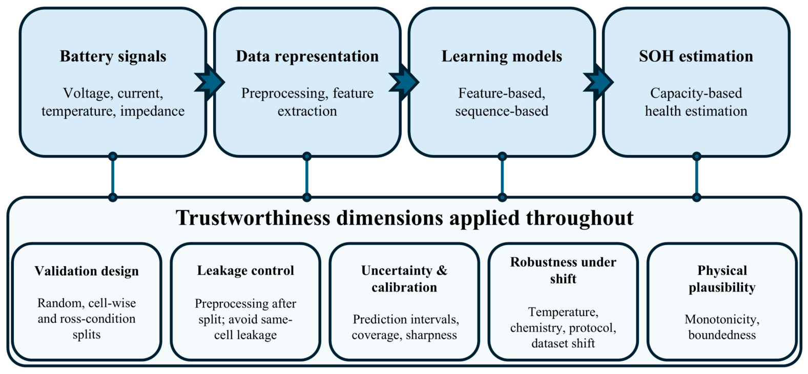
This review focuses specifically on lithium-ion batteries and, within that scope, on machine-learning-based SOH estimation using data-driven and hybrid methods built from observable electrical signals and their temporal histories. Remaining useful life (RUL) prediction is included only when it appears as an auxiliary task in multi-task SOH models. Purely electrochemical ageing models, non-learning Kalman filter and observer-based methods, battery materials synthesis, manufacturing process optimisation, and thermal runaway analysis are excluded unless they directly support machine-learning-based SOH estimation. This narrower scope allows a deeper discussion of how SOH models are formulated, how their reported performance is validated, and how their uncertainty is assessed. The literature is organised by learning formulation rather than algorithm family, so that validation rigour, leakage risk, and uncertainty calibration are treated as primary methodological criteria rather than secondary considerations [32]. Handcrafted feature and sequence-based pipelines are evaluated by their accuracy, uncertainty handling, calibration requirements, robustness across operating conditions, and efficiency under limited labelled data [33]. Figure 1 summarises the review framework adopted in this paper, in which the validation design, leakage control, uncertainty calibration, robustness under distribution shift, and physical plausibility are treated as cross-cutting criteria throughout the SOH estimation workflow.

The remainder of the review is organised as follows: Section 2 presents the mathematical formulations of battery health learning, Section 3 discusses data representations and learning models, Section 4 examines robustness, uncertainty, and trustworthiness, and Section 5 synthesises guidelines and open problems.

2. Mathematical Formulations of Battery Health Learning

Battery SOH estimation is naturally introduced as supervised regression because measured battery signals are paired with continuous reference SOH values. However, it is not an ordinary regression because the voltage, current, temperature, and impedance-related measurements are indirect observations of degradation [34], while capacity-based SOH labels are usually obtained from controlled reference measurements or periodic reference tests [7]. Thus, uncertainty arises from sensor measurements and preprocessing choices, from label definition and reference-test design [35], from path-dependent ageing history, and from shifts in cell chemistry, temperature, or duty cycle [36]. The formulations in this section clarify what is predicted, what information is available, and why regression, sequence learning, and uncertainty-aware validation are needed for trustworthy SOH estimation.

2.1. Notation, Inputs, and Targets

Let $\mathbf{x}\in {\mathbb{R}}^d$ denote a feature vector extracted from one charge–discharge cycle, a partial charging segment, or a fixed operational window of a lithium-ion cell. This vector represents observable battery behaviour under a particular sensing and preprocessing pipeline, rather than the true degradation state itself. Depending on the sensing and preprocessing pipeline, x may contain statistical summaries, voltage–capacity descriptors, resistance-related indicators, voltage relaxation parameters, thermal features, or learned embeddings from raw signals [37,38,39,40,41]. Let

$${\mathbf{X}}_{\left(1:T\right)}=\left({\mathbf{x}}_1,\dots ,{\mathbf{x}}_T\right)$$

(1)

denote a temporal sequence of such representations over $T$ cycles. This distinction is important because a single vector $\mathbf{x}$ gives a snapshot of battery behaviour, whereas ${\mathbf{X}}_{\left(1:\mathrm{T}\right)}$ retains part of the degradation history. Since the battery ageing is path-dependent, the present SOH may depend not only on the current cycle but also on the preceding usage history. For capacity-based SOH, the primary target is often a scalar $y\in [0,1]$, defined as the ratio between the current available capacity and the nominal or initial capacity [42]. Here, $y$ should be interpreted as a reference test-based label rather than a perfectly observed latent health variable. Auxiliary targets may include an internal resistance-related target $r\in {\mathbb{R}}_{+}$, RUL $\tau \in {\mathbb{Z}}_{+}$ measured in cycles to end-of-life [43], or a discrete degradation stage label $c\in \{1,\dots ,K\}$ [44]. Capacity-based SOH remains the dominant target of the current learning-based battery health studies [45], although the exact measurement protocol affects the label semantics [35]. The general task is to learn a mapping:

$$f:\mathcal{X}\to \mathcal{Y}$$

(2)

where $\mathcal{X}$ may be a Euclidean feature space, a sequence space, or a hybrid representation combining engineered and learned features. This mapping approximates battery health from incomplete, noisy, and condition-dependent observations. In the simplest point-estimation setting,

$$\widehat{y}=f(\mathbf{x})$$

(3)

whereas in a temporal setting, one writes

$${\widehat{y}}_t=f\left({\mathbf{X}}_{t-w+1:t}\right)$$

(4)

where $w$ denotes the observation window, and ${\widehat{y}}_t$ denotes the predicted SOH at cycle $t$. Thus, the point-estimation formulation uses the information contained in a single cycle, segment, or feature representation, whereas the temporal formulation uses recent degradation history to reduce ambiguity caused by path-dependent ageing.

2.2. SOH Estimation as Supervised Regression

Supervised regression is the natural starting point when each battery cycle, partial segment, or engineered feature vector can be paired with a reference SOH label. This formulation is appropriate because capacity-based SOH is usually represented as a continuous quantity, such as normalised available capacity, rather than as a discrete class [46]. Thus, the learning task is to estimate a continuous health value from measured battery behaviour. In the battery setting, however, this label is not an error-free observation of health; it is affected by reference-test design, measurement noise, and the operating conditions under which the label was obtained [47,48]. Once this signal-to-SOH pairing is defined, a labelled dataset can be written as

$$\mathcal{D}=\{({\mathbf{x}}_i,y_i){\}}_{i=1}^n$$

(5)

with samples drawn from a joint distribution $P(\mathbf{x},y)$. The objective is to find an estimator $\widehat{f}$ minimising the expected risk

$$R(f)={\mathbb{E}}_{(\mathbf{x},\mathrm{y})\sim \mathbf{P}}[\mathcal{l}(f(\mathbf{x}),y)]$$

(6)

where $\mathcal{l}$ is typically the squared error or absolute error loss. This risk formalises average prediction error, but by itself it does not describe whether an individual prediction is reliable, whether the residual error is input-dependent, or whether the model will remain valid under a new cell or operating condition. In practice, this becomes empirical risk minimisation,

$${\widehat{R}}_n(f)={\displaystyle \frac{1}{n}}{\displaystyle \sum _{i=1}^n}\mathcal{l}(f({\mathbf{x}}_i),y_i)+\lambda \mathsf{\Omega }(f)$$

(7)

where $\mathsf{\Omega }(f)$ is a regularisation term that controls model complexity. This formulation covers many methods used in battery SOH estimation, including linear models, kernel methods, tree-based methods, and neural networks [49]. Richardson et al. [50], for example, cast battery health forecasting in a related supervised-learning setting, using cycle index as input, normalised capacity as output, and a latent function model with additive noise. This makes the noise term explicit, whereas many point-estimation studies report only average error and leave predictive uncertainty implicit. However, the assumptions commonly used to analyse empirical risk minimisation do not hold cleanly for battery data [51]. Successive cycles from the same cell are temporally correlated, and observations are naturally grouped by cell [52]. Moreover, training and deployment conditions may differ in temperature, protocol, chemistry, or usage history [26]. As a result, generalisation guarantees derived under independent and identically distributed (i.i.d.) assumptions may be overly optimistic unless the validation design accounts for temporal dependence, grouped structure, and domain shift [53]. Low observed error under weak evaluation settings may therefore reflect interpolation within a narrow regime rather than genuine out-of-domain predictive ability [54]. More generally, target-domain error depends not only on source-domain error but also on the divergence between the source and target domains and on whether a predictor can perform well across both [55]. In battery SOH estimation, this issue appears directly in transfer learning settings, where the target domain data are limited and differ in distribution from the source domain data [41]. Thus, the supervised-regression formulation is useful as a baseline mathematical model, but trustworthy SOH estimation also requires explicit attention to label uncertainty, grouped temporal dependence, and source–target mismatch.

2.3. Sequence-Learning Formulations

Feature-based and sequence-based SOH estimation represent two different modelling views. A feature-based model estimates battery health from one cycle, one partial segment, or one engineered descriptor, and therefore treats the input as a snapshot of the battery state. A sequence-learning model instead uses a recent history of observations and estimates SOH from the evolution of battery behaviour over time. Because battery ageing is path-dependent, this history-based formulation is useful when a single-cycle representation is insufficient to distinguish between cells with similar present measurements but different degradation trends [6]. When the input is represented not as a fixed feature vector but as a recent history of observations, SOH estimation becomes a sequence-learning problem. Let

$${\mathbf{X}}_{t-w+1:t}=\left({\mathbf{x}}_{t-w+1},\dots ,{\mathbf{x}}_t\right)$$

(8)

denote a sliding window of length $w$. A sequence-to-scalar estimator takes the form

$$f:{\mathbb{R}}^{w\times d}\to \mathbb{R}, {\widehat{y}}_t=f\left({\mathbf{X}}_{t-w+1:t}\right)$$

(9)

where the model uses the recent observation window to estimate the current SOH. This formulation is appropriate when the aim is to infer the present health state from the recent degradation history. A prognostic estimator may instead take the form

$$g:{\mathbb{R}}^{w\times d}\to {\mathbb{R}}^h,\hspace{1em}\hspace{1em}{\widehat{\mathbf{y}}}_{t+1:t+h}=g\left({\mathbf{X}}_{t-w+1:t}\right)$$

(10)

producing future SOH or other health-related quantities over a horizon $h$. Thus, sequence learning can be used either for current SOH estimation or for forecasting the future degradation trajectory. The main mathematical distinction between feature-based and sequence-based formulations lies in where temporal information is compressed or learned. In feature-based pipelines, one first defines a projection.

$$\phi :{\mathbb{R}}^p\to {\mathbb{R}}^d,\hspace{1em}\hspace{1em}d\ll p$$

(11)

that compresses raw signal trajectories into lower-dimensional health indicators. This makes the model more data-efficient and interpretable, but it also means that the temporal information retained by the model is limited by the chosen feature design. Sequence models, by contrast, preserve richer temporal structures and rely on an architectural bias to identify the informative patterns. Shen et al. [41] provide a direct example from battery SOH estimation; their deep convolutional neural network (DCNN)-based capacity estimator learns from multi-dimensional time-series measurements collected during partial charging. Transfer learning is then used to improve estimation when labelled target domain data are limited. Mathematically, this shifts a part of the modelling burden from the hand-engineered features to the learned hierarchical representations [56]. A related extension appears in BatLiNet, which moves from single-cell sequence learning to inter-cell relational learning [57]. By comparing a target cell with a reference cell, BatLiNet illustrates how sequence-learning formulations can be extended beyond single-cell prediction under diverse ageing conditions.

2.4. Multi-Task and Weakly Physics-Guided Formulations

Several recent studies move beyond single-task SOH regression [58,59]. The motivation is that SOH is only one observable summary of a broader degradation process. Related quantities, such as RUL, degradation stage, or resistance growth, can provide additional constraints on the latent health representation. One route is multi-task learning, in which SOH is estimated jointly with related outputs such as RUL, degradation stage, or another health proxy [59]. A generic formulation is

$${\mathcal{L}}_{mt}(\theta )={\alpha }_1{\mathcal{L}}_{\mathrm{SOH}}(\theta )+{\alpha }_2{\mathcal{L}}_{\mathrm{aux}}(\theta )+\lambda {\parallel \theta \parallel }_2^2$$

(12)

In this formulation, ${\alpha }_1$ and ${\alpha }_2$ denote fixed task weights. However, fixed weighting may be suboptimal when the associated prediction tasks differ in scale, noise level, or label reliability. Following the homoscedastic uncertainty-weighting formulation of Kendall et al. [60], the fixed task weights can be replaced by the learned task-uncertainty parameters. For the two regression-type battery health objectives, an adapted form is

$$L_{mt}\left(\theta ,{\sigma }_1,{\sigma }_2 \right)={\displaystyle \frac{1}{2{\sigma }_1^2}}{L}_{SOH}\left(\theta \right)+{\displaystyle \frac{1}{2{\sigma }_2^2}} L_{aux}\left(\theta \right)+log{\sigma }_1+log{\sigma }_2+\lambda {\parallel \theta \parallel }_2^2$$

(13)

Here, ${\sigma }_1$ and ${\sigma }_2$ represent task-dependent uncertainty parameters. This formulation reduces reliance on manually selected task weights and is relevant when SOH, RUL, resistance-growth, or degradation-stage objectives differ in magnitude, label quality, or physical variability. For mixed regression and classification objectives, the same principle can be expressed through task-specific likelihood terms. The auxiliary term acts as a structural regularizer by encouraging shared latent representations to preserve information relevant to more than one degradation-related target. Ma et al. [40] provide a direct example by combining differential thermal voltammetry (DTV)-based features with recurrent neural networks for joint SOH estimation and RUL prediction. This frames battery health learning as a coupled prediction problem rather than an isolated scalar regression. A second route is weakly physics-guided learning, in which the model remains data-driven but incorporates partial physical structure [39]. This formulation is useful when the data alone are insufficient to identify a stable health mapping, but available battery knowledge can restrict the model toward physically plausible solutions. Physical knowledge may be introduced in two ways: explicitly, through equivalent-circuit-derived features extracted from the relaxation-voltage segment, and implicitly, through degradation-aware constraints in the training objective. In abstract form,

$$\mathbf{z}=\mathrm{F}\left(\mathbf{x},\mathbf{u}\right),\hspace{1em}\hspace{1em}\widehat{y}=\mathcal{G}\left(\mathbf{z}\right)$$

(14)

where $\mathbf{x}$ is the measured signal segment, and $\mathbf{u}$ is a vector of physically meaningful features. The loss is then no longer only a data-fitting term;

$${\mathcal{L}}_{data}={\displaystyle \frac{1}{n}}{\displaystyle \sum _{i=1}^n}{\left({y_i-\widehat{y}}_i\right)}^2$$

(15)

and the full loss becomes

$$\mathcal{L}={\mathcal{L}}_{data}+\beta {\mathcal{L}}_{phys}$$

(16)

where ${\mathcal{L}}_{phys}$ encodes battery-degradation structure in the embedding or output space. Lanubile et al. [38] provide a complementary example at the feature-design level. Their domain-knowledge-guided framework constructs online-computable SOH indicators from EV-like operating data, emphasising physical relevance and real-time deployability. More generally, degradation-aware physical constraints can act as regularizers that steer data-driven models toward physically consistent solutions without requiring a full electrochemical simulator [61]. In practice, such a structure may take the form of feature design, smoothness constraints, monotonicity assumptions, or degradation-aware penalties.

2.5. Sources of Statistical Difficulty

Several sources of statistical difficulty recur across battery health learning. These difficulties explain why the formulations above cannot be treated as ordinary regression models with clean inputs and labels. First, nonstationarity arises because battery degradation is a drifting process, so the joint distribution changes with age [62],

$$P_t\left(\mathbf{x},y\right)\ne P_{t^{\prime }}\left(\mathbf{x},y\right),\hspace{1em}\hspace{1em}t\ne t^{\prime }$$

(17)

Second, heteroscedastic noise occurs when measurement and process noise variances are not constant and may vary across batteries and operating conditions [63].

$$\mathrm{V}\mathrm{a}\mathrm{r}(Y\mid \mathbf{X}=\mathbf{x})={\sigma }^2(\mathbf{x})$$

(18)

Third, cell-to-cell variability means that even nominally identical cells can diverge because of subtle manufacturing or initialisation differences [64]. Fourth, covariate shift arises when the input distribution differs between training and test conditions, for example, because of changes in temperature or duty cycle [65], as expressed by

$$P_{\mathrm{train}}(\mathbf{x})\ne P_{\mathrm{test}}(\mathbf{x})$$

(19)

Fifth, label scarcity arises because collecting accurate SOH labels is time-consuming and laborious [17]. Sixth, label ambiguity remains because SOH reference values and end-of-life criteria depend on the chosen test protocol [4]. These sources of difficulty interact in practice. Attia et al. [66] show that even early-life-cycle prediction is difficult because degradation is nonlinear and variable across cells despite controlled conditions. Greenbank and Howey [67] likewise show that forecasting capacity fade, knee point, and end of life depend strongly on the selection of informative features, because many degradation drivers are only indirectly observable. Taken together, these issues make battery health learning a structured statistical problem rather than a generic regression benchmark.

2.6. Evaluation Metrics and Validation Protocols

Evaluation metrics and validation protocols determine how reported SOH prediction performance should be interpreted. Point-error metrics quantify average numerical accuracy, whereas interval metrics and validation design indicate whether predictions remain reliable under uncertainty, cell-to-cell variation, and distribution shift. For point prediction, the most common metrics are

$$\mathrm{M}\mathrm{A}\mathrm{E}={\displaystyle \frac{1}{n}}{\displaystyle \sum _{i=1}^n}\mid y_i-{\widehat{y}}_i\mid ,\hspace{1em}\hspace{1em}\mathrm{R}\mathrm{M}\mathrm{S}\mathrm{E}=\sqrt{{\displaystyle \frac{1}{n}}{\displaystyle \sum _{i=1}^n}(y_i-{\widehat{y}}_i{)}^2}$$

(20)

$$\mathrm{M}\mathrm{A}\mathrm{P}\mathrm{E}={\displaystyle \frac{100}{n}}{\displaystyle \sum _{i=1}^n}\mid {\displaystyle \frac{y_i-{\widehat{y}}_i}{y_i}}\mid ,\hspace{1em}\hspace{1em}{R}^2=1-{\displaystyle \frac{\sum _i(y_i-{\widehat{y}}_i{)}^2}{\sum _i(y_i-\overline{y}{)}^2}}$$

(21)

For uncertainty-aware models that output interval-valued predictions, coverage and normalised width are commonly used metrics. If a model outputs a prediction interval $\left[L_i,U_i\right]$, then prediction interval coverage probability (PICP) and a normalised interval-width measure can be defined as follows [68]:

$$\mathrm{P}\mathrm{I}\mathrm{C}\mathrm{P}={\displaystyle \frac{1}{n}}{\displaystyle \sum _{i=1}^n}\mathbf{1}\{y_i\in [L_i,U_i]\},$$

(22)

$$\mathrm{P}\mathrm{I}\mathrm{N}\mathrm{A}\mathrm{W}={\displaystyle \frac{1}{nR}}{\displaystyle \sum _{i=1}^n}(U_i-L_i),$$

(23)

where $R$ denotes the range of the target values. Richardson et al. [50] are a useful example in this context because they formulate SOH forecasting as a Bayesian nonparametric problem and emphasise uncertainty-aware forecasting rather than point prediction alone. Greenbank and Howey [67] further show that credible intervals may appear sharp while still failing nominal calibration targets. Accordingly, studies that model uncertainty should report point-error metrics together with calibration and interval-sharpness measures [25,69]. The evaluation protocol is equally important because it determines what a reported error actually supports [22]. The validation protocols considered in this review are summarised in

Table 1. Validation protocols for battery SOH estimation and the type of generalisation they assess.

Protocol	Description	Tests for	Rigour
Random split	Cycles from all cells are mixed and split at random	Interpolation only	Lowest
Temporal split	Train on early cycles and test on later cycles from the same cell	Within-cell extrapolation in time	Low–Medium
Leave-one-cell-out	Train on N − 1 cells and test on a held-out cell	Cell-to-cell generalisation	Medium
Cross-condition	Train and test under different temperatures or duty cycles	Covariate-shift robustness	High
Cross-dataset	Train on dataset A and test on dataset B	Dataset-shift robustness	High
Leave-one-condition-out	Train on all but one operating regime and test on the held-out regime	Distributional robustness	Highest

, ordered by increasing stringency. The reported error, therefore, has meaning only relative to the split protocol that generated it. PICP and PINAW, defined above, evaluate prediction intervals specifically; their relationship to broader probabilistic calibration measures such as ECE and negative log-likelihood is clarified in Section 4.3.

2.7. Why Reported Performance Can Be Misleading

Several recurring sources of performance inflation appear in battery health studies, including train–test leakage across cycles from the same cell, same-cell memorisation under temporal continuity, preprocessing leakage before splitting, and evaluation under overly homogeneous protocols. In these cases, the reported error reflects performance under the chosen split, not necessarily performance under deployment conditions. Let the reported test error be

$${\widehat{R}}_{\mathrm{test}}\left(\widehat{f}\right)$$

(24)

When the test set is too similar to the training set, this quantity may seriously underestimate the true deployment risk.

$$R_{\mathrm{deploy}}\left(\widehat{f}\right)$$

(25)

The practically relevant quantity is therefore

$${\Delta }_{\mathrm{deploy}}=R_{\mathrm{deploy}}\left(\widehat{f}\right)-{\widehat{R}}_{\mathrm{test}}\left(\widehat{f}\right)$$

(26)

A large value of ${\Delta }_{\mathrm{deploy}}$ means that the model appears accurate under the reported evaluation protocol but loses reliability when applied to new cells, operating regimes, or datasets. Ben-David et al. [55] make this concern precise through the source–target bound

$${ϵ}_T\left(h\right)\le {ϵ}_S\left(h\right)+{\displaystyle \frac{1}{2}}{d}_{H\Delta H}\left(D_S,D_T\right)+\lambda$$

(27)

where ${ϵ}_T(h)$ and ${ϵ}_S(h)$ denote the target- and source-domain errors of hypothesis $h$, $d_{H\Delta H}(D_S,D_T)$ measures the discrepancy between the source and target distributions, and $\lambda$ denotes the joint error of the best hypothesis on the source and target domains. This shows that strong source-domain performance is insufficient when source and target domains differ. In battery terms, a model can perform well under weak splits yet fail under new cells, altered duty cycles, or different chemistries.

Table 2. Representative studies showing how reported battery health prediction performance varies with validation protocol.

Richardson et al. (2017) [50] SOH forecasting/RUL	Protocol Type: Same-cell temporal forecasting: train on capacity data up to the current cycle and forecast the remainder; evaluated across multiple training proportions rather than a single arbitrary split.
	Reported Error: Uses two RMSE-based measures over multiple forecasting horizons: $RMS{E}_Q$ for capacity-trajectory error and $RMS{E}_{\mathrm{E}\mathrm{o}\mathrm{L}}$ for end-of-life prediction error. In the multi-output example, one two-output model gives $RMS{E}_{\mathrm{E}\mathrm{o}\mathrm{L}}=4.86,$ whereas a weaker-correlated two-output model gives $RMS{E}_{\mathrm{E}\mathrm{o}\mathrm{L}}=18.1.$
	What It Shows: Rigorous horizon-based same-cell forecasting is stronger than a single arbitrary split, but it is still not a cross-cell robustness test.
Shen et al. (2020) [41] Capacity/SOH estimation	Protocol Type: Cell-wise five-fold cross-validation: whole cells held out for testing; each fold uses 4 test cells from a 20-cell target dataset.
	Reported Error: Test RMSE = 1.503% for DCNN-ETL; comparators: RF 3.528%, GP 3.300%, DCNN 2.616%, DCNN-TL 2.095%, DCNN-EL 3.680%.
	What It Shows: Strong example of cross-cell evaluation with whole-cell separation; better than random sample splitting because full cells are held out.
Lanubile et al. (2024) [38] SOH/capacity estimation	Protocol Type: Leave-one-cell-out in Scenario 2: train on all cells except the test cell, then test on the held-out cell.
	Reported Error: With energy-based features, absolute percentage error is below 1.5% in Scenario 2; even Scenario 1 remains below 2.5% on the other four cells.
	What It Shows: Useful evidence that physically meaningful features can generalise across held-out cells, though still within a small-cell study.
Greenbank and Howey (2021) [67] Capacity trajectory/knee point/EOL	Protocol Type: Cell-wise repeated holdout with cross-validation: training and test cells fully separated, repeated 20 times.
	Reported Error: In the representative 5-feature setting: median RMSEQ = 0.83%, median EOL error = 1.3%, median knee-point error = 2.6%; 95% of profiles had RMSEQ < 3.1%.
	What It Shows: A good example of stringent cell separation: low capacity error is still possible, but harder downstream targets, such as the knee point, degrade more.
Paulson et al. (2022) [70] Early lifetime prediction	Protocol Type: Leave-one-condition-out: one cathode chemistry held out entirely as unseen during the outer loop.
	Reported Error: For 100-cycle features: MAE = 78 cycles when all cathodes are represented in training, but unseen-chemistry performance degrades strongly; for the unseen-cathode set, overall errors reach MAE = 230/191 cycles and RMSE = 297/286 cycles for ExtraTrees/NuSVR, respectively.
	What It Shows: A direct demonstration that a distributional shift to unseen chemistry can substantially degrade performance.
Zhang et al. (2025) [57] Early lifetime prediction	Protocol Type: Cross-dataset/broad multi-condition evaluation across MATR-1, MATR-2, HUST, MIX-100, and MIX-20.
	Reported Error: BatLiNet reduces the RMSE of the best baseline by 36.5%, 6.8%, 20.1%, 27.4%, and 40.1% across the five datasets; it also reduces the average MAPE by up to 40% relative to its single-cell CNN counterpart. However, MIX-100 and MIX-20 are explicitly reported as harder than narrower datasets such as MATR-1 and MATR-2.
	What It Shows: Strong evidence that broad-condition evaluation is materially harder than restricted-condition evaluation, even for a strong model.

Note: ${\mathrm{R}\mathrm{M}\mathrm{S}\mathrm{E}}_{\mathrm{Q}}$ = root mean squared error for capacity-trajectory prediction; ${\mathrm{R}\mathrm{M}\mathrm{S}\mathrm{E}}_{\mathrm{E}\mathrm{o}\mathrm{L}}$ = root mean squared error for end-of-life prediction; RF = random forest; GP = Gaussian process; DCNN = deep convolutional neural network; ETL = ensemble transfer learning; TL = transfer learning; EL = ensemble learning; NuSVR = nu-support vector regression.

summarises representative quantitative evidence from primary studies.

The evidence in Table 2 supports the central methodological point of this review, namely that the reported battery health performance is highly protocol-dependent. The same-cell temporal forecasting and cell-wise cross-validation may yield low error, but performance often deteriorates under unseen chemistries, broader ageing diversity, or cross-dataset evaluation, where the train–test distribution shift is more severe.

3. Data Representations and Learning Models

Data representation affects the reliability of an SOH model as much as the model architecture itself. The same error value can support different claims depending on how labels are defined, how diverse the cells and operating conditions are, and whether uncertainty estimates and calibration are evaluated under held-out or shifted test conditions.

3.1. Benchmark Datasets and Label Definitions

Most machine-learning studies on battery SOH estimation rely on a limited number of publicly available cycling datasets. These datasets differ in chemistry, number of cells, cycling protocol, temperature range, and measurement procedure, and such differences affect both model development and the interpretation of the reported performance [19,20]. Dataset choice therefore constrains the scope of any accuracy, uncertainty, or robustness claim. A model evaluated on a small number of cells may support the within-dataset conclusions, but it provides limited evidence about calibration or reliability under cell-to-cell, temperature, chemistry, or protocol shift. The NASA Prognostics Centre of Excellence dataset is widely used as a baseline resource for SOH estimation studies [71]. The CALCE repository is also frequently used because it includes a broader variation in chemistry and cycling protocol, although the number of cells within each condition remains limited [72]. The Oxford Battery Degradation Dataset is often used when more realistic drive-cycle-style loading profiles are of interest [73]. The MIT–Stanford fast-charging dataset is widely used for early-life prediction and cross-cell learning because it contains a comparatively large number of lithium-iron-phosphate cells tested under multiple fast-charging policies [37]. Additional public datasets, including Panasonic and recent high-power characterisation datasets, extend coverage to other chemistries and operating conditions [74,75]. SOH is most commonly defined as the ratio of present discharge capacity to nominal or initial capacity under a standardised reference test [42]. Because this label usually requires a controlled charge–discharge procedure, it is not directly available during normal operation and must be obtained from periodic reference measurements or related reconstruction procedures. The meaning of the label, therefore, depends not only on battery condition but also on the test protocol used to measure it [35,42]. This matters for uncertainty-aware evaluation because a narrow prediction interval is less informative if the reference SOH value depends on temperature, rest period, current rate, or capacity-test protocol. A further source of inconsistency is the end-of-life threshold. Although 80% of the nominal capacity is commonly adopted, the threshold may vary across applications and studies, which complicates the direct comparison of reported results and the transfer across datasets [8,35]. Thus, the benchmark results should be interpreted together with the label definition, test protocol, and operating conditions under which the reported uncertainty and error values were obtained.

3.2. Feature-Based Representations and Compatible Models

Feature engineering maps a raw charge–discharge cycle to a lower-dimensional descriptor vector, $\varphi (\mathrm{cycle})\in {\mathbb{R}}^d$. In SOH estimation, this transformation introduces a domain-informed structure by retaining degradation-relevant information while reducing measurement noise and cycle-to-cycle variation unrelated to battery health [18,70]. At the same time, feature engineering also determines what uncertainty can be represented: information removed during feature extraction cannot later be recovered by the regression model. For feature-based methods, point-error metrics are incomplete unless the associated uncertainty estimates are also tested for calibration under held-out cells, operating conditions, or datasets. Common feature categories include voltage-curve descriptors, incremental capacity (IC) and differential voltage (DV) features, resistance-related indicators, and cycle-level summary statistics [3,13,18]. Voltage-curve descriptors include charging time to a voltage threshold, constant-voltage duration, and voltage at a fixed state of charge. IC and DV features are derived from $dQ/dV$ and $dV/dQ$ curves, where peak position, peak height, and peak area are often associated with electrode degradation processes. Because IC/DV features require numerical differentiation, their stability depends strongly on the treatment of measurement noise, voltage quantisation, and irregular sampling. A mathematically explicit stabilisation step is to smooth the capacity–voltage relation before differentiation. If $Q(V)$ denotes the measured capacity–voltage curve, a Gaussian-smoothed curve can be written as $\tilde{Q}(V)=(G_{\sigma }\ast Q)(V)$, where $G_{\sigma }(s)=(1/\sqrt{2\pi }\sigma )\mathrm{e}\mathrm{x}\mathrm{p}[-s^2/(2{\sigma }^2)]$ is a Gaussian kernel and $\ast$ denotes convolution. The corresponding stabilised IC representation is $d\tilde{Q}/dV$, while second-derivative quantities such as $d^2\tilde{Q}/d{V}^2$ may be used when curvature, peak broadening, or inflexion behaviour is informative. Analogously, DV features can be stabilised by smoothing $V(Q)$ before computing $d\tilde{V}/dQ$. The kernel width $\sigma$ controls the bias–variance trade-off. Insufficient smoothing amplifies derivative noise, whereas excessive smoothing can attenuate degradation-related peaks. Resistance-related indicators can be obtained from voltage transients during current steps or from impedance-based measurements, while cycle-level statistics may include temperature summaries, energy throughput, and relaxation-voltage drift.

Model choice depends strongly on the structure of the resulting feature vector. Linear models such as ridge regression, least absolute shrinkage and selection operator (LASSO), and elastic net remain useful when the feature space is moderate in dimension, and the number of labelled cells is limited. In battery SOH studies, these models are valued for their interpretability and for their role as transparent baselines against which more complex estimators can be compared [49,76]. LASSO is additionally useful when feature sparsity is desirable because its ${\mathcal{l}}_1$ regularisation can suppress redundant predictors. However, standard linear models are primarily point estimators unless an explicit probabilistic error model, Bayesian formulation, or post hoc interval method is added. Their apparent transparency should therefore not be confused with calibrated uncertainty. Under cross-cell or cross-condition testing, residual variance may change with the operating regime, so intervals estimated from one condition may be too narrow or too wide in another.

Kernel methods such as support vector regression (SVR) and Gaussian process regression (GPR) are commonly used when nonlinear relations between engineered features and SOH are expected. These methods can represent a nonlinear structure without explicitly constructing high-dimensional basis expansions. SVR is usually used as a point estimator in SOH studies, so prediction intervals require additional assumptions or post hoc calibration. In battery applications, GPR is especially important because it provides predictive mean and variance within a single probabilistic model [9,77,78]. This is a stronger uncertainty mechanism than simply attaching intervals after training, but it is not automatically sufficient. GPR uncertainty depends on the kernel, noise model, and training-domain coverage; predictive variance may be poorly calibrated when the test cell, temperature, chemistry, or cycling protocol differs from the training data. Kernel choice is particularly important because it encodes prior assumptions about the smoothness of the SOH–feature relation. The radial basis function (RBF) kernel, $k_{\mathrm{R}\mathrm{B}\mathrm{F}}(x,x^{\prime })={\sigma }_f^2\mathrm{e}\mathrm{x}\mathrm{p}[-\parallel x-x^{\prime }{\parallel }^2/(2{\mathcal{l}}^2)]$, assumes an infinitely differentiable latent function and therefore favours very smooth degradation trajectories. In contrast, the Matérn kernel, $k_{\nu }\left(x,x^{\prime }\right)={\sigma }_f^2{\displaystyle \frac{2^{1-\nu }}{\mathsf{\Gamma }(\nu )}}{\left(\sqrt{2\nu }\parallel x−x^{\prime }\parallel /\mathcal{l}\right)}^{\nu }{K}_{\nu }\left(\sqrt{2\nu }\parallel x−x^{\prime }\parallel /\mathcal{l}\right)$, introduces a smoothness parameter $\nu$. Smaller values of $\nu$ allow rougher functions and may better represent abrupt slope changes, knee-like behaviour, or regime transitions in battery ageing. Thus, kernel selection affects not only point prediction but also posterior variance, extrapolation behaviour, and interval calibration. Therefore, GPR-based SOH studies should report not only root mean squared error (RMSE) or mean absolute error (MAE), but also empirical coverage and interval width under cross-cell or cross-condition splits. The main limitation of kernel methods is computational cost, which increases rapidly with the number of training observations and can restrict direct application to larger datasets.

Tree-based ensembles, including random forests and boosting methods, partition the feature space through recursive splits and are well-suited to structured, feature-engineered inputs. In battery SOH studies, they are attractive because they can model nonlinear interactions, tolerate irrelevant variables better than many parametric models, and usually require less feature scaling than kernel or neural methods [49,79]. Their effectiveness on tabular data is also consistent with broader findings in machine learning that tree ensembles remain competitive, and often superior, on structured datasets [80]. For uncertainty, however, standard tree ensembles require caution. Variation across trees or boosted learners can be used as a heuristic uncertainty signal, but it does not by itself guarantee calibrated predictive intervals. When interval estimates are needed, additional methods such as ensemble-based intervals, quantile regression, or conformal calibration must be introduced and then evaluated through coverage and sharpness.

Overall, feature-based models are often data-efficient and easier to audit than high-capacity sequence models, but their uncertainty claims depend strongly on the evaluation protocol. A feature-based model that performs well under a random or same-cell split may still produce unreliable intervals under held-out cells, changed temperatures, or cross-dataset transfer. For this reason, feature-based SOH studies should report point accuracy together with uncertainty coverage, interval width, and calibration behaviour under the same validation protocol used to claim robustness.

3.3. Sequence Representations and Compatible Models

Sequence-based approaches use voltage, current, temperature, or related multichannel signals directly as the model input rather than compressing each cycle into a handcrafted feature vector. This changes the representation from a fixed-dimensional descriptor to a time-indexed sequence or matrix, thereby preserving local waveform structure and temporal ordering [33]. This has direct implications for uncertainty: most sequence models used in SOH estimation are deterministic point predictors unless uncertainty is introduced through additional mechanisms such as Monte Carlo dropout, deep ensembles, Bayesian variants, quantile losses, or conformal calibration. Therefore, low point error from a sequence model should not be interpreted as evidence of calibrated uncertainty unless coverage and interval width are explicitly evaluated.

One-dimensional convolutional neural networks (1D CNNs) apply learned filters along the time axis and are therefore suited for extracting local patterns from charge or discharge segments. In battery SOH estimation, they are commonly used to learn voltage- or current-segment representations without an explicit manual feature construction [41,56,81]. Their receptive field is local, unless enlarged through deeper stacking or dilation. Mathematically, the receptive field determines the number of input samples that can influence a given output representation [82]. For a stack of $L$ one-dimensional convolutional layers with kernel size $k_{\mathcal{l}}$ and stride $s_{\mathcal{l}}$, the effective receptive field can be expressed as

$$R_L=1+{\displaystyle \sum _{\mathcal{l}=1}^L}\left(k_{\mathcal{l}}-1\right){\displaystyle \prod _{j=1}^{\mathcal{l}-1}}{s}_j$$

(28)

In dilated convolutions, the kernel size can be replaced by the effective kernel size $k_l^{\mathrm{e}\mathrm{f}\mathrm{f}}=1+(k_l-1)d_l$, where $d_l$ is the dilation factor. In the common stride-one case with dilation, this gives $R_L=1+{\sum }_{l=1}^L(k_l-1)d_l$. If the signal is sampled with an interval $\Delta t$, the temporal span covered by the convolutional representation is approximately $R_L\Delta t$. This span should be chosen in relation to the temporal correlation length of the voltage, current, or temperature signal. If $R_L\Delta t$ is shorter than the degradation-relevant temporal pattern, the model may miss long-range dependencies. If it is much longer than the informative correlation scale, the model may introduce unnecessary parameters and become more sensitive to overfitting. Temporal convolutional networks extend this idea by increasing receptive field length while maintaining efficient parallel computation, which makes convolution-based sequence models attractive when local degradation signatures are informative. Convolutional sequence models do not natively provide predictive distributions. Intervals derived from dropout sampling or ensembles can be useful, but they require calibration checks because local waveform patterns may shift with temperature, SOC window, current profile, or sensor preprocessing.

Recurrent networks, especially long short-term memory (LSTM) and gated recurrent unit (GRU) models, represent sequential dependence through hidden-state updates governed by the gating mechanisms. In battery applications, these models are widely used when the order of observations within a cycle or across cycles is expected to carry degradation information [2,40,83]. Their main advantage is the direct modelling of sequential dependence without requiring fixed handcrafted descriptors. Their limitations include higher training costs than simple convolutional models and weaker efficiency on very long sequences. Recurrent models may also become overconfident when the test trajectory differs from the training trajectories. Their hidden states can encode protocol-specific temporal patterns, so cross-cell and cross-condition validation is necessary before interpreting their predictions or intervals as robust.

Transformers use self-attention to model pairwise dependence across sequence positions and therefore do not rely on recurrent state propagation. In battery studies, they have been applied to both intra-cycle signals and longer degradation histories [84,85]. Their main strength is flexible long-range dependency modelling, but this comes with a higher computational cost and, in practice, greater sensitivity to data availability. For this reason, their advantages are more evident when training data are comparatively rich or when transfer learning is available [33]. Attention weights should also not be treated as uncertainty estimates. Transformer-based SOH models generally require the same uncertainty additions as other deep sequence models, and their calibration may deteriorate under chemistry, temperature, protocol, or dataset shift if such shifts are not represented during training.

Across these representation–model pairs, the main design issue is the balance between model flexibility and data efficiency. Handcrafted feature representations reduce the input dimension and can stabilise the estimation when the number of labelled cells is limited, but they restrict the model to patterns selected during feature design. Sequence models retain more of the original signal structure and can learn task-specific representations directly from data, but this flexibility increases the risk of overfitting in small-sample settings [33,45]. Sequence-based SOH studies should report point accuracy together with uncertainty coverage, interval sharpness, calibration behaviour, and performance under held-out cells or operating conditions. Without these checks, improved accuracy from CNN, recurrent, or transformer models may reflect stronger interpolation within familiar trajectories rather than reliable degradation assessment under the deployment shift.

3.4. Transfer, Adaptation, and Physics-Guided Approaches

Battery datasets are often too limited in size or operating-condition coverage to support reliable training of high-capacity models from scratch. One response is transfer learning, in which a model is first trained on source cells or source conditions and then adapted to a target setting with limited labelled data. In battery SOH estimation, this approach is motivated by the assumption that some degradation-related representations remain useful across cells, protocols, or operating regimes even when the final input–output relation changes [21]. Battery-specific applications include recurrent and related transfer-learning formulations for SOH prediction under limited target-domain supervision [86]. Transfer from laboratory conditions to field operation has also been studied explicitly [65]. Transfer learning mainly addresses robustness under limited target data, but it does not automatically provide calibrated uncertainty. If the target domain is sparsely labelled, the transferred model may reduce average error while still producing overconfident predictions or intervals that are too narrow for the new operating regime.

A related strategy is domain adaptation, which is used when source labels are available but target labels are limited or unavailable. The central idea is to reduce the discrepancy between source and target representations so that a predictor trained on the source domain remains useful on the target domain. In battery SOH studies, this has been implemented through adversarial transfer learning [15], domain adaptation across electrochemistry and working conditions [24], unsupervised domain adaptation [87], and feature alignment under shallow-cycle conditions [88]. Label-free multi-domain adaptation has also been reported [89]. These methods are effective only when a transferable representation exists. When source and target domains differ too strongly in chemistry, degradation mechanism, or sensing regime, the assumption of useful alignment becomes weaker. Therefore, domain adaptation should be evaluated not only by target-domain point error but also by whether uncertainty coverage and interval width remain acceptable on held-out cells, temperatures, chemistries, or cycling protocols. Representation alignment can reduce distributional mismatch, but it does not by itself guarantee calibrated predictive uncertainty.

Self-supervised pretraining addresses label scarcity from a different direction. Instead of relying first on labelled source data, the model is trained to learn signal representations from unlabeled battery sequences and only later fine-tuned for SOH prediction. In battery studies, this idea has been explored to reduce the dependence on expensive ground-truth labels [17]. The broader methodological basis for this strategy is well established in machine learning [90]. Its practical value in battery applications depends on whether the pretraining objective captures the structures relevant to degradation. Self-supervised representations may improve data efficiency, but the resulting SOH predictor is still usually a point model unless a probabilistic output layer, ensemble, quantile objective, or conformal calibration step is added. Thus, label efficiency and calibrated uncertainty should be treated as separate properties.

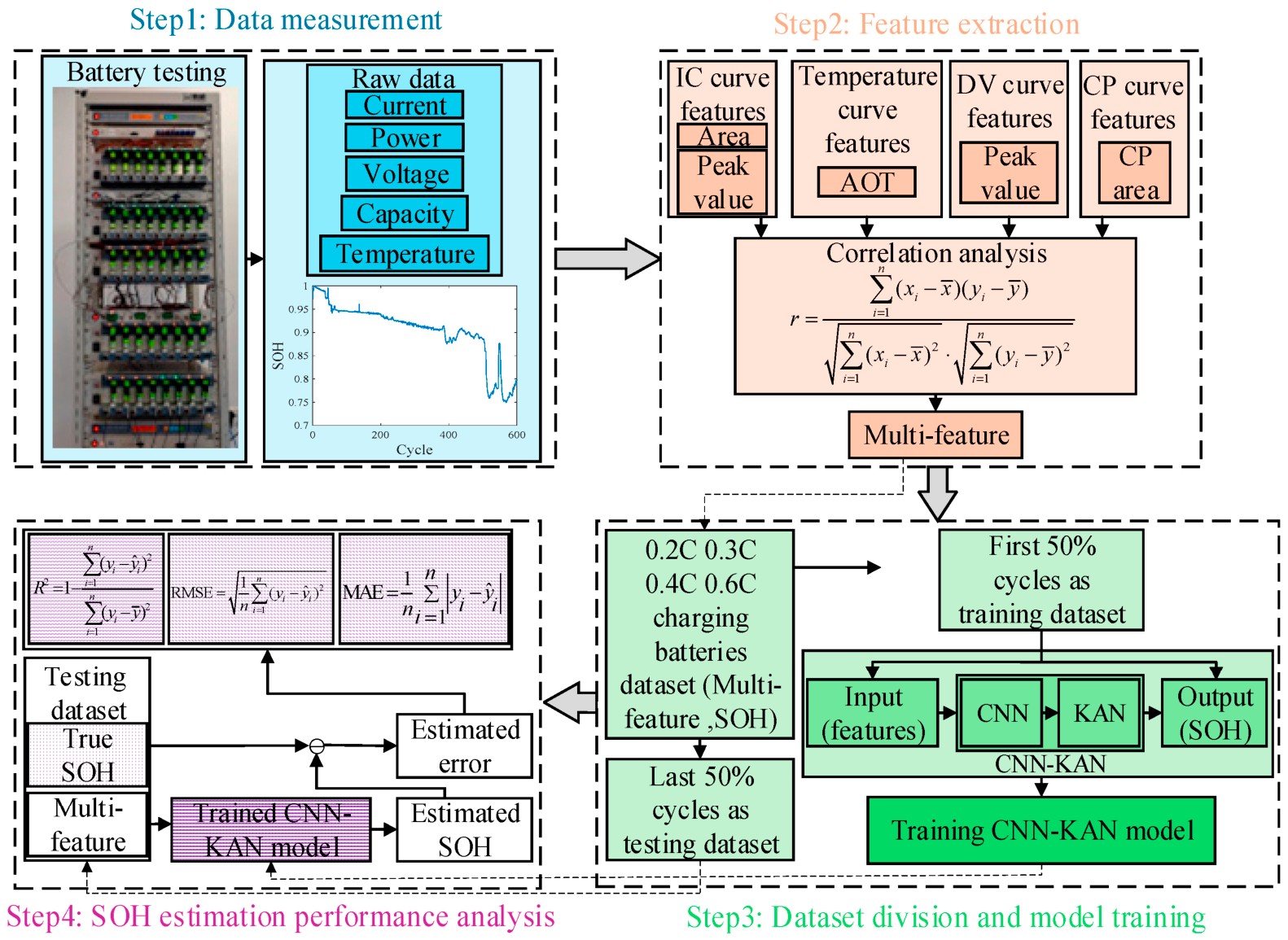
A further line of work incorporates physical knowledge into statistical learning without requiring full electrochemical modelling. In this review, such methods are treated as weakly physics-guided approaches because the model remains data-driven, but its representation, loss function, or output behaviour is constrained by physical considerations. Domain knowledge-guided feature construction has been used to improve SOH estimation from operational data [38]. Partial-segment modelling with physical guidance has also been reported [39]. Related formulations include physics-informed architectures designed specifically for SOH estimation [91] and generic physics-informed frameworks for lithium-ion battery SOH modelling [92]. These approaches are particularly relevant when labelled data are limited and purely data-driven models are prone to overfitting. Physical constraints can improve plausibility, for example, by discouraging unrealistic degradation trajectories or outputs outside physically meaningful ranges. However, physical plausibility is not the same as calibrated uncertainty. If the imposed physical prior is incomplete or condition-dependent, the model may appear more stable while still being miscalibrated under unseen operating regimes. Physics-guided SOH studies should therefore report physical consistency together with empirical coverage, interval sharpness, and robustness under cross-cell or cross-condition validation. Figure 2 [93] is included as a representative example of a conventional hybrid SOH estimation workflow, including battery measurement, curve-based feature extraction, dataset division, convolutional neural network Kolmogorov–Arnold network (CNN-KAN) model training, and point-error evaluation. It should not be interpreted as the complete trustworthiness framework proposed in this review. Rather, it illustrates the modelling pipeline commonly used in current SOH studies, while the evaluation stage should be supplemented by the cross-cutting trustworthiness checks shown in Figure 1 and operationalised across model families in

Table 3. Qualitative comparison of model families for SOH estimation with emphasis on uncertainty handling, calibration requirements, and robustness under distribution shift.

Model Family	Usual SOH Use	Uncertainty Mechanism	Calibration and Interval Issue	Robustness Under Shift	Recommended Reporting
Linear/Ridge/Elastic Net [76,94]	Feature-based point regression with transparent coefficients	Usually point prediction; uncertainty requires an explicit residual model, Bayesian variant, or post hoc interval method	Interpretability does not imply calibrated uncertainty; residual variance and interval coverage should be checked when intervals are reported	Depends strongly on whether engineered features remain stable across cells and operating conditions	MAE/RMSE, residual analysis, interval coverage and width if uncertainty is claimed
SVR/GPR [77,78]	Nonlinear regression on engineered features	GPR provides predictive mean and variance natively; SVR usually requires additional interval construction	GPR variance depends on kernel, noise model, and training-domain coverage; empirical coverage and interval sharpness are still required	Kernel assumptions may become unreliable under new cells, temperatures, chemistries, or cycling protocols	Point error, empirical coverage, interval width, and cross-cell or cross-condition results
Tree Ensemble [79]	Nonlinear regression on structured feature vectors	Tree or ensemble disagreement can be used as a heuristic uncertainty signal; quantile, ensemble, or conformal methods may be added	Ensemble spread alone does not guarantee calibrated prediction intervals	May perform well on structured data but can still overfit dataset-specific feature distributions	Point error, coverage, sharpness, and validation under held-out cells or conditions
CNN (1D) [81,95]	Learned local temporal patterns from voltage, current, or temperature segments	Usually deterministic; uncertainty is commonly added through MC dropout, ensembles, quantile loss, or conformal calibration	Added intervals require explicit calibration checks; low point error does not imply reliable uncertainty	Sensitive to waveform changes caused by SOC window, temperature, current profile, or preprocessing	Point error, uncertainty coverage, interval width, calibration, and shifted-condition testing
LSTM/GRU [83]	Sequential degradation modelling within or across cycles	Usually deterministic; uncertainty requires MC dropout, ensembles, Bayesian variants, quantile objectives, or conformal methods	Hidden-state models may be overconfident if test trajectories differ from training trajectories	May encode protocol-specific temporal patterns and fail under changed ageing histories	Point error, calibration, coverage, sharpness, and held-out-cell/condition validation
Transformer [84]	Long-range sequence modelling using attention	Usually deterministic; attention weights are not uncertainty estimates	Predictive intervals require additional uncertainty methods and empirical calibration	Data requirements and shift sensitivity can be high when chemistries, protocols, or datasets change	Point error, uncertainty method, calibration results, and cross-dataset or cross-condition testing
Transfer Learning/DA [21,26,96]	Adaptation from source cells or conditions to limited target data	Uncertainty is inherited from the base model unless explicitly added	Representation alignment does not guarantee calibrated target-domain uncertainty	Can reduce source–target mismatch, but may fail when chemistry, sensing, or degradation mechanisms differ strongly	Source–target split details, target error, uncertainty coverage, interval width, and target-domain calibration
Physics-informed [91,92]	Data-driven prediction constrained by physical features, losses, or priors	Task-dependent; physical constraints improve plausibility but do not necessarily provide predictive distributions	Physical consistency is not equivalent to calibrated uncertainty	Robustness depends on whether the physical prior remains valid under the target operating condition	Point error, physical consistency checks, calibration, coverage, sharpness, and cross-condition validation

Note: The table summarises methodological properties and recommended checks. It does not imply that every cited study reported all listed uncertainty, calibration, or robustness metrics.

, including leakage control, cross-cell or cross-condition validation, uncertainty calibration, interval coverage and sharpness, robustness under distribution shift, and physical plausibility.

Table 3 provides a qualitative methodological comparison of the model families discussed in this section, with emphasis on uncertainty handling, calibration requirements, and robustness under shifted evaluation. The purpose is not to identify a universally best model but to clarify which methods provide uncertainty natively, which require post hoc uncertainty estimation, and which claims require additional calibration or cross-condition validation.

4. Robustness, Uncertainty, and Trustworthiness

Trustworthy SOH estimation requires that robustness, uncertainty, calibration, interpretability, and physical plausibility be assessed together rather than as isolated properties. These dimensions are examined below with emphasis on their implications for deployment under shifted operating conditions.

4.1. Domain Shift and Out-of-Distribution Generalisation

A central difficulty in battery SOH estimation is the mismatch between the training and deployment distributions. This mismatch may take several forms. Under covariate shift, changes in temperature, current profile, SOC window, or charging protocol alter $P(x)$ while leaving $P(y\mid x)$ approximately stable. Under prior shift, the marginal distribution of health states changes, for example, when one dataset contains mostly early-life cells, and another contains many late-life or fast-aged cells. Under concept shift, the conditional relation $P(y\mid x)$ itself changes, as may happen across chemistries, manufacturers, sensing regimes, or battery formats. In domain-adaptation terms, low source-domain error alone is insufficient because target performance also depends on domain divergence and joint cross-domain learnability [55]. The same issue also affects uncertainty: an interval or predictive variance calibrated on the source domain may become miscalibrated when the test cell, temperature, chemistry, or duty cycle changes.

The battery literature contains several explicit responses to this problem. Liu et al. [24] use adversarial domain adaptation across electrochemistry and operating conditions and report average SOH estimation error within 4.77%, with more than 30% of the improvement attributed to domain adaptation itself. Qiu et al. [87] propose unsupervised domain adaptation based on encoded subspace distance for differences in chemistry, profile, and ambient temperature. Chen et al. [88] use multi-kernel mean maximum discrepancy (MMD) in the self-attention knowledge domain adaptation network (SKDAN) framework to transfer knowledge from labelled full cycles to unlabeled shallow cycles, reporting RMSE below 2% across several SOC ranges and operating conditions. Zhao et al. [89] combine adversarial multi-domain adaptation with relaxation-voltage features and report strong error reduction across temperature-transfer and material-transfer scenarios. Together, these studies show that the domain shift is already a practical barrier to a robust SOH transfer.

Methodologically, current battery studies concentrate on two main remedy families. The first is domain-adversarial learning, which seeks representations that predict SOH while making source and target domains difficult to distinguish. The second is distribution alignment, most commonly through MMD or related discrepancy penalties, with correlation alignment (CORAL) sometimes used as a benchmark. However, battery-specific evaluation remains uneven because many studies still evaluate only on a fixed source–target pair known during training rather than on genuinely unseen deployment conditions. Moreover, improved target-domain point error is not equivalent to reliable target-domain uncertainty; coverage, interval width, and calibration should also be evaluated after adaptation. By contrast, explicit test-time adaptation and distributionally robust optimisation remain scarce in the battery SOH literature reviewed here. Thus, despite growing recognition of domain shift, relatively few studies test robustness under conditions resembling true out-of-distribution deployment, and even fewer assess whether uncertainty estimates remain calibrated under such shifts.

4.2. Uncertainty Quantification

Robust SOH estimation requires not only a point estimate $\widehat{y}(x)$, but also a predictive distribution. In Bayesian formulations, one places a posterior over parameters,

$$p(\theta \mid \mathcal{D})\propto p(\mathcal{D}\mid \theta )p(\theta )$$

(29)

and then computes the predictive distribution

$$p(y^{\ast }\mid {\mathbf{x}}^{\ast },\mathcal{D})=\int p(y^{\ast }\mid {\mathbf{x}}^{\ast },\theta ) p(\theta \mid \mathcal{D}) d\theta$$

(30)

Here, $\mathcal{D}$ denotes the training data, $\theta$ denotes the model parameters, and $\left(x^{\ast },y^{\ast }\right)$ denotes a test input and its corresponding SOH target. This separates predictive uncertainty into epistemic uncertainty, arising from limited knowledge of the model and reducible with more data, and aleatoric uncertainty, arising from irreducible noise. In battery health prediction, probabilistic machine-learning approaches remain a developing direction, and recent reviews emphasise the importance of explicitly characterising predictive uncertainty [25]. The practical issue is not only whether an interval is produced, but whether the interval is calibrated, sufficiently sharp, and reliable under the validation protocol used to support the SOH claim.

A common approximation in battery SOH uncertainty modelling is Monte Carlo dropout, which uses dropout-based sampling to approximate predictive uncertainty [97]. Its appeal lies in simple implementation and moderate computational cost, although the resulting intervals are not always evaluated rigorously. A related practical strategy is repeated stochastic retraining [98], where the confidence intervals are obtained from multiple random-seed runs of the same architecture. Such intervals may be operationally useful, but they should not automatically be interpreted as calibrated Bayesian uncertainty. Another important family is deep ensembles, where multiple independently initialised models are trained, and their predictive disagreement is used as an uncertainty signal. Lakshminarayanan et al. [99] show that deep ensembles can provide high-quality predictive uncertainty and can express higher uncertainty on out-of-distribution inputs than standard point-prediction networks. This makes them especially relevant for battery SOH under chemistry, temperature, and protocol shift, although explicit battery-specific deep-ensemble studies remain limited. For these sampling- or ensemble-based methods, uncertainty quality must still be checked through empirical coverage, interval width, and calibration under held-out cells or shifted operating conditions.

Among battery-specific methods, Gaussian-process-based approaches remain among the clearest uncertainty models because they provide predictive mean and variance natively. Richardson et al. [50] formulate SOH forecasting probabilistically, while Zhang et al. [100] combine a temporal convolutional network-based feature extraction with the GPR and obtain

$$P(C^{\ast }\mid V,C,{\mathbf{v}}^{\ast })\sim \mathcal{N}({\mu }^{\ast },{\Sigma }^{\ast })$$

(31)

Here, $C^{\ast }$ denotes the predicted capacity or SOH-related target, $v^{\ast }$ denotes the test input feature vector, and ${\mu }^{\ast }$ and ${\Sigma }^{\ast }$ are the predictive mean and variance, respectively. Thus, a 95% interval is given by ${\mu }^{\ast }\pm 1.96\sqrt{{\Sigma }^{\ast }}$. This is a strong battery example because uncertainty is tied to an explicit probabilistic model rather than only to the repeated heuristic sampling. Even in this case, however, predictive variance should not be assumed to be calibrated under cross-condition or cross-dataset deployment without empirical verification. Quantile regression and conformal prediction provide alternative routes for constructing prediction intervals. Quantile regression estimates conditional quantiles $Q_{\alpha }(y\mid \mathbf{x})$ directly through the pinball loss and avoids explicit distributional assumptions. Conformal prediction constructs intervals $C_{\alpha }(\mathbf{x})$ satisfying

$$P\{y\in C_{\alpha }(\mathbf{x})\}\ge 1-\alpha$$

(32)

Here, $C_{\alpha }(\mathbf{x})$ denotes the prediction set or interval at miscoverage level $\alpha$. Under exchangeability, conformal prediction is mathematically attractive because its coverage guarantee does not require the predictive model to be correctly specified [101]. However, for battery SOH estimation, exchangeability may fail under cross-condition and cross-chemistry deployment. Conformal methods are therefore promising, but their assumptions must be discussed explicitly in shift-dominated settings.

4.3. Calibration, Sharpness, and Decision Usefulness

For SOH regression, calibration means that the stated predictive uncertainty agrees with observed error frequencies. For an interval forecast with nominal coverage $1-\alpha$, calibration can be assessed empirically as

$${\widehat{c}}_{\alpha }={\displaystyle \frac{1}{n}}{\displaystyle \sum _{i=1}^n}1\left\{y_i\in \left[L_i^{\alpha },U_i^{\alpha }\right]\right\}\approx 1-\alpha$$

(33)

Here, $[L_i^{\alpha },U_i^{\alpha }]$ denotes the prediction interval for sample $i$, and ${\widehat{c}}_{\alpha }$ is the empirical coverage. Equivalently, for a nominal 1 − α prediction interval, calibration means that the long-run proportion of true values falling inside that interval equals 1 − α. To harmonise the terminology used across this review, uncertainty metrics can be grouped according to the type of predictive output. For interval forecasts, empirical coverage denotes the observed proportion of true SOH values that fall inside the reported prediction intervals. PICP is the corresponding interval-forecast coverage metric, while interval width and PINAW describe how wide or informative those intervals are; PINAW is the normalised form of interval width, and sharpness is the general term for this property. Therefore, interval-valued SOH studies should at least report the nominal interval level, PICP or empirical coverage, and interval width or PINAW. Coverage and sharpness must always be reported together, since wide intervals can trivially achieve high coverage. For full probabilistic forecasts, where a model outputs a predictive distribution rather than only an interval, reliability diagrams, ECE-style summaries, and negative log-likelihood are more appropriate. Reliability diagrams and ECE assess whether predicted confidence levels agree with observed frequencies, whereas negative log-likelihood evaluates the probability assigned to the observed SOH value. Guo et al. [102] apply the calibration criterion in Equation (33) to motivate reliability diagrams and scalar calibration summaries such as expected calibration error (ECE). In practice, calibration is assessed empirically rather than exactly, with reliability diagrams comparing empirical frequencies with predicted confidence levels, and ECE summarising the deviation between them. Negative log-likelihood provides a related proper scoring rule that penalises overconfident errors.

Calibration alone, however, is not sufficient. For battery management, a 95% interval spanning 5 percentage points of SOH may be statistically acceptable yet operationally unhelpful, whereas an interval spanning 1 percentage point of SOH may be much more useful for maintenance and safety decisions. This motivates sharpness, that is, interval width, as a second criterion. A model that achieves nominal coverage only by producing wide intervals offers limited decision value. Therefore, uncertainty mechanisms such as GPR variance, Monte Carlo dropout, ensembles, quantile regression, or conformal intervals should be compared using the same coverage-and-sharpness criteria.

The battery-specific uncertainty literature illustrates this trade-off clearly. Zhang et al. [100] report narrow confidence intervals together with strong coverage behaviour, whereas Geng et al. [98] provide visually plausible intervals without a formal calibration audit. Thelen et al. [25] similarly note that uncertainty should be judged not only by whether intervals are reported, but also by whether they are statistically reliable and sufficiently informative. Accordingly, trustworthy SOH uncertainty requires coverage together with sharpness. This joint requirement remains under-assessed in much of the battery literature, where interval plots are often presented without reliability diagrams, ECE-style summaries, or explicit nominal-versus-empirical coverage comparisons.

4.4. Interpretability and Physical Plausibility

Interpretability in battery SOH estimation may be approached through feature importance, SHAP values, gradient-based saliency, and attention visualisation. Geng et al. [98] provide a useful recent example: they apply Deep SHAP to an attention–LSTM model and show both local and global feature attributions, identifying physically meaningful charging-curve features as dominant contributors to SOH prediction. This is valuable because it links model decisions to observable degradation-related variables rather than leaving the predictor as a purely opaque black box. However, attribution-based explanations should not be interpreted as uncertainty estimates or calibration evidence. A model may highlight physically meaningful inputs while still producing overconfident predictions, poorly calibrated intervals, or unstable behaviour under shifted operating conditions.

Interpretability alone is not sufficient and should be paired with physical plausibility checks. At a minimum, a deployable SOH model should satisfy four conditions. First, predicted SOH should decrease or remain approximately flat over ageing cycles, apart from noise-level fluctuations, and should not exhibit spurious recovery. Second, predictions should remain within the physically meaningful range, typically [0, 1] or its equivalent percentage representation. Third, predictions should be stable under physically irrelevant perturbations, such as harmless timestamp shifts, superficial protocol-label differences, or equivalent reparameterizations of the same signal. Fourth, when queried beyond the support of the training data, the model should fail gracefully rather than collapse into implausible outputs. These checks complement, rather than replace, uncertainty calibration and cross-condition validation. These checks are rarely reported systematically in the battery SOH literature. Lanubile et al. [38] move in this direction by introducing physically meaningful SOH indicators grounded in battery behaviour, whereas Wang et al. [17] improve SOH estimation through feature-enhanced self-supervised learning with weak labels; however, a standardised plausibility audit remains largely absent. That gap matters because interpretability alone does not guarantee physical plausibility, and physical plausibility alone does not guarantee calibrated uncertainty or robustness under deployment shift.

4.5. Failure Modes in Battery Machine Learning

Several recurring failure modes in battery machine learning can be stated more precisely in statistical terms. Extrapolation failure occurs when a model is queried in a region where the training density is effectively negligible, that is, $p_{\mathrm{train}}(\mathbf{x})\approx 0$. In such regions, the learned function is only weakly constrained by data, so late-life predictions based on early-life training may be unstable or arbitrarily biassed. This is especially relevant when rapid degradation phases or knee-point behaviour are absent from training. Uncertainty estimates should ideally widen in such regions; if they remain narrow, the model is not only inaccurate but also miscalibrated. Shortcut learning arises because empirical risk minimisation tends to exploit any correlation that reduces training error, including non-causal or non-transferable ones. In the language of invariance, the model may rely on spurious features that are predictive in one environment but unstable across environments, rather than on invariant degradation-related structure. Arjovsky et al. [103] make this point sharply by minimising training error alone, which encourages learning all available correlations, not only the stable ones. In battery settings, cycle index, protocol-specific artefacts, or benchmark-specific preprocessing cues may all serve as shortcuts when the training distribution is narrow. Dataset bias is a related failure mode in which a predictor overfits to the data-generating protocol of a benchmark rather than to a transferable battery health structure. In that case, the model becomes adapted to one empirical distribution and exhibits high variance under domain shift [55]. Such models may still produce low error and apparently sharp intervals under random or same-cell splits while becoming unreliable under held-out cells or operating conditions. Catastrophic forgetting appears in continual or sequential adaptation, where updating a model on a new target domain degrades performance on previously learned domains [104]. Its mathematical cause is interference in shared parameters: gradient updates that reduce loss on the new domain may increase loss on older ones. For uncertainty-aware SOH estimation, continual adaptation also requires recalibration; an uncertainty model fitted to an earlier domain may no longer provide valid coverage after the predictor is updated. Hyperparameter sensitivity reflects the high variance of model selection under small validation sets, where a claimed performance gain may depend strongly on one favourable split or one tuning path. This is particularly important in battery ML, where datasets are often small and repeated-seed reporting remains inconsistent. Taken together, these failure modes reflect statistical instability under limited, structured, and shifted data rather than isolated engineering inconveniences.

4.6. Defining Trustworthy SOH Estimation

The literature reviewed here suggests that trustworthy SOH estimation should be judged by verifiable methodological criteria rather than low average error alone [25,38,39,50,70]. On this basis, trustworthy SOH estimation can be defined through five requirements. First, results should be reported under at least a cross-cell or cross-condition split that tests genuine generalisation. Second, predictive intervals should be provided whenever uncertainty is claimed, and those intervals should be checked for empirical calibration and useful sharpness. Third, performance should be demonstrated under at least one concrete form of distribution shift, such as temperature, chemistry, SOC window, or dataset transfer. Fourth, preprocessing, hyperparameters, and training procedures must be specified well enough for replication, and code and data should ideally be made public. Fifth, predictions should remain bounded, degradation-consistent, and insensitive to physically irrelevant perturbations. This definition is intentionally stricter than a ranking based on point-error metrics alone. A model that performs well on one benchmark under a weak split, produces visually appealing but uncalibrated intervals, and offers no evidence under distribution shift should not be called trustworthy, even if its RMSE is low. Conversely, a model with slightly worse average error but clearer uncertainty behaviour, stronger shift evaluation, and basic physical sanity checks is more credible for deployment.

5. Synthesis, Guidelines, and Open Problems

5.1. Cross-Study Comparison

Across the reviewed literature, the most common pipeline remains supervised regression with a capacity-based SOH target, using either handcrafted charge/discharge features or short sequence representations as inputs. At the representation level, the field remains divided between feature-based pipelines, which stay competitive in low-data settings, and deep sequence models such as CNN–LSTM and Transformer-like encoders. A clearer pattern, however, concerns generalisation rather than architecture alone. Current evidence suggests that some of the strongest reported cross-condition robustness comes from models that combine domain adaptation or physics-guided structure with mechanistically informed feature extraction [33]. A related gap is that uncertainty is not reported consistently across model families: some studies provide only point-error metrics, some provide prediction intervals without calibration analysis, and relatively few report coverage, sharpness, and calibration under shifted validation protocols. Thus, methods are now distinguished less by architecture alone than by evaluation under genuinely shifted deployment conditions and by the credibility of their uncertainty estimates. A second synthesis point is methodological rather than architectural. Papers evaluated under in-dataset or same-cell settings often report very low errors, whereas broader-condition or cross-domain studies typically report larger but more realistic errors. This reflects the shift from interpolation to distributionally shifted generalisation. The same distinction applies to uncertainty: intervals that appear reliable under the same-cell evaluation may not retain nominal coverage under cross-condition or cross-dataset testing.

Table 4. Reported prediction error ranges stratified by validation protocol across selected reviewed studies.

Validation Protocol	No. Studies	Reported MAE Range	Reported RMSE Range
Random split	1	0.52–0.53%	0.58–0.68%
Temporal split	1	0.75–2.90%	1.02–4.80%
Leave-one-cell-out	3	Not consistently reported	0.83–1.50%
Cross-condition	4	1.39–3.20%	1.47–3.57%
Cross-dataset	2	1.66–2.98%	1.85–3.37%

summarises the subset of reviewed studies for which the split protocol and standard error metrics were sufficiently clear to allow protocol-stratified comparison.

The main result is the trend itself: performance generally looks best under weaker in-dataset or temporal protocols and worsens under cross-condition or cross-dataset transfer. Error values, therefore, must be interpreted relative to the generalisation claim implied by the split. Because calibration and interval metrics are not reported consistently across these studies, the table should not be read as a complete comparison of trustworthiness. Rather, it shows why point-error ranges alone are insufficient and why future comparisons should pair MAE/RMSE with uncertainty coverage, interval width, and calibration under the same validation protocol.

5.2. Recommended Benchmark Design

A future benchmark for battery SOH estimation should be designed around the deployment question rather than around what is easiest to evaluate. At a minimum, such a benchmark should require cross-cell evaluation, since a model that has never been tested on held-out cells has not demonstrated cell-to-cell generalisation. It should also include at least one cross-condition experiment, in which training and test data differ in temperature, load profile, charging window, C-rate, or another operating factor known to affect the input distribution. This is the minimum needed to test robustness under a plausible field shift. For uncertainty-aware models, these same splits should also be used to evaluate empirical coverage, interval width, and calibration; uncertainty assessed only under random or same-cell splits does not establish deployment reliability. Benchmarks should also include a transparent baseline model, such as ridge regression or GPR on a standardised feature set, so that improvements from more complex architectures can be interpreted against a meaningful anchor rather than only against other deep models. Where uncertainty is claimed, the baseline should include an uncertainty-capable comparator, such as GPR or a calibrated interval method, so that interval quality is compared as well as point accuracy. Every benchmark study should include ablation experiments that isolate the contribution of preprocessing, feature extraction, architecture, loss design, and adaptation strategy. Without ablations, it is difficult to determine whether gains arise from methodological novelty or changed data handling. For probabilistic or interval-valued methods, ablations should also clarify whether improved performance comes from the predictor itself, the uncertainty-estimation method, or a post hoc calibration step. Statistical comparison should be based on repeated resampling or repeated training runs, followed by appropriate significance testing [105]. For two-model comparisons, the Wilcoxon signed-rank test is a reasonable default, whereas Friedman-style tests with post hoc analysis are more appropriate across multiple models and datasets [106]. A final benchmark-design principle concerns openness. The benchmark should specify not only the data partitions but also the exact preprocessing order, especially whether normalisation, smoothing, and window construction are performed before or after splitting. This is a major leakage pathway in battery studies and should be controlled by design rather than corrected retrospectively. The same transparency is needed for uncertainty evaluation. Studies should report how prediction intervals were constructed, whether calibration was performed on a separate calibration set, and whether the calibration set is independent of the final test cells or conditions.

5.3. Reporting Checklist for Future Papers

To improve comparability, we propose the following minimum reporting standard for future battery SOH studies. First, the dataset should be described explicitly, including chemistry, number of cells, cycling protocol, voltage window, and temperature range. Second, the target definition should be stated precisely, including the SOH formula, end-of-life threshold, and the reference test procedure used to obtain labels. Third, the preprocessing pipeline should be fully disclosed, including normalisation, smoothing, resampling, alignment, windowing, and whether each operation was carried out before or after train–test splitting. Fourth, the split protocol should be stated concretely, including which cells or conditions appear in each partition. Fifth, the model specification should include architecture, hyperparameters, optimiser, stopping criterion, and tuning procedure. Sixth, the evaluation protocol should report at minimum MAE and RMSE, and for probabilistic methods, also PICP, PINAW, empirical coverage, interval sharpness, the uncertainty-estimation method, and evidence of calibration under the stated validation protocol. If calibration or conformal prediction is used, the calibration data should be identified separately from the final test cells or conditions. Seventh, the computational footprint should include training time, inference time, hardware, and approximate model size. Eighth, a reproducibility statement should declare whether code, data, and scripts are available. When robustness is claimed, the reporting should also specify the shift being tested, such as held-out cells, temperature change, chemistry transfer, SOC-window change, or cross-dataset evaluation. This checklist is intentionally modest because it does not require a specific algorithmic philosophy, only a minimum level of transparency. Even this standard would substantially improve the reproducibility and interpretability of the current literature.

5.4. Method Selection Under Realistic Constraints

Method choice should depend on the deployment regime rather than on benchmark popularity. With small labelled datasets, feature-based models such as GPR, gradient-boosted trees, or carefully regularised transfer-learning pipelines remain strong choices because they impose stronger inductive structure and tend to have lower estimation variance than large sequence models in the small-sample regime. When uncertainty estimates are required in such settings, GPR or calibrated interval methods provide a more defensible starting point than deterministic models that only report point error. Fully deep sequence models may still perform well, but they are more vulnerable to overfitting unless source-domain transfer, strong priors, or careful feature compression are available. Their use should therefore be accompanied by uncertainty checks, such as empirical coverage, interval width, and calibration under held-out cells or operating conditions. When labels are noisy or protocol-dependent, squared-error loss can be overly sensitive to outliers because its penalty grows quadratically with error magnitude. In that regime, robust losses such as Huber or quantile losses are preferable, and small numerical gains under fragile label definitions should not be over-interpreted. Quantile losses are especially relevant when interval prediction is desired, but the resulting intervals still require calibration assessment. In online BMS deployment with limited compute, lightweight models remain attractive because latency, memory, and recalibration cost become binding constraints. A slightly less accurate model with stable millisecond-scale inference may be more useful than a heavier model with prohibitive deployment cost. For deployment, computational efficiency should therefore be considered together with calibration maintenance, since uncertainty estimates may need periodic recalibration as the operating distribution changes. For cross-condition deployment, domain adaptation, transfer learning, or weakly physics-guided regularisation are currently among the most defensible strategies because they directly address train–test mismatch rather than assuming it away. However, such methods should be evaluated on held-out conditions rather than on held-out cells from the same operating regime. Improved target-domain accuracy should also be accompanied by evidence that uncertainty coverage and interval sharpness remain acceptable after adaptation. For pack-level estimation, the problem becomes qualitatively harder because aggregation introduces additional variance from cell imbalance and heterogeneity; mathematically, the target is no longer a simple cell-level latent variable but a function of interacting cell states. Since pack-level evidence remains much thinner than cell-level evidence, claims of general deployment readiness should be made cautiously.

5.5. Open Problems and Future Directions

A first open problem is the development of formal transfer-learning guarantees that are genuinely useful for battery data. Domain-adaptation theory already provides source–target risk bounds, but these have not yet been translated into practical criteria for deciding when a source domain is similar enough to help and when transfer is likely to become negative. The obstacle is that divergence terms such as $H\Delta H$-type discrepancies or representation-level distribution gaps are difficult to estimate tightly from finite samples in high-dimensional battery feature spaces. As a result, the resulting bounds are often too loose to guide deployment decisions. Battery studies such as Qiu et al. [87] already show that larger domain discrepancy makes transfer harder and can constrain the upper bound of adaptation benefit; the remaining challenge is to turn that insight into a practically useful criterion. A related need is to connect transferability criteria with uncertainty calibration, because a source domain may improve point accuracy while still producing miscalibrated uncertainty in the target domain.

A second open direction is self-supervised and label-efficient learning. Recent weak-label and self-supervised battery studies show that useful transfer is possible even when only a small amount of target-labelled data is available [17]. Active learning is closely related. When reference tests are expensive, cells should not be labelled uniformly. Instead, the most informative cells should be selected. Active learning can improve annotation efficiency by selecting samples through uncertainty or diversity rather than passive sampling [107]. For SOH estimation, an important open question is whether these strategies improve not only point accuracy but also calibrated uncertainty under held-out cells, operating conditions, and datasets.

A third problem is continual learning and deployment monitoring. Real systems age, conditions drift, and a deployed model should ideally adapt without erasing previously useful knowledge. Catastrophic forgetting is therefore not an abstract machine-learning problem, but a direct deployment issue for battery models updated online or across fleets. Kirkpatrick et al. [104] show one influential route, namely protecting parameters that are important to earlier tasks, yet battery-specific continual-learning formulations remain sparse. This should be coupled with online recalibration of uncertainty and out-of-distribution detection. In practical BMS deployment, recalibration should be treated as an ongoing process rather than a one-time validation step, because both the input distribution and the degradation mechanism may change over time.

A fourth promising direction is weak physics integration. Monotonicity constraints, degradation-rate regularisation, symmetry-aware augmentation, and physically meaningful health indicators offer a practical middle ground between unconstrained black-box learning and full electrochemical simulation. The key question is not whether prior knowledge helps, but how strongly it should be enforced when the available physics is approximate or condition-dependent. Future physics-guided models should therefore report physical consistency together with uncertainty coverage, interval sharpness, and cross-condition robustness, rather than treating physical plausibility as a substitute for calibration. In that sense, future progress is likely to come less from isolated architectural novelty than from better evaluation, stronger robustness testing, and principled integration of structured prior knowledge.

6. Conclusions

Machine-learning-based state-of-health estimation for lithium-ion batteries has developed substantially, but the literature still shows important limitations in validation rigour, comparability, uncertainty reporting, and deployment relevance. This review examined the field in terms of mathematical formulation, data representation, model selection, evaluation protocol, uncertainty quantification, robustness, and trustworthiness, with emphasis on the conditions under which reported performance can be interpreted meaningfully. Several main findings emerge from the reviewed studies. First, classical feature-based methods and deep sequence models serve different but complementary purposes. Feature-based methods remain competitive in small-data settings because they are data efficient, easier to audit, and often more stable under limited labels, whereas deep sequence models become more attractive when richer temporal data, adequate training diversity, and stronger evaluation settings are available. Second, reported performance is strongly affected by validation design, preprocessing strategy, and train–test mismatch. Weak split protocols, preprocessing leakage, and limited cross-condition evaluation can produce errors that are not representative of performance under broader operating variation. Third, uncertainty quantification is necessary for deployment-oriented SOH estimation, but prediction intervals are useful only when accompanied by empirical calibration, coverage, and sharpness analysis. Fourth, weak physics-guided structure offers a practical way to improve plausibility and generalisation while retaining the flexibility of data-driven learning, but physical plausibility should not be treated as a substitute for calibrated uncertainty. Taken together, the reviewed evidence indicates that progress in battery SOH estimation should not be assessed by lower prediction error alone. A trustworthy SOH model should demonstrate generalisation across cells and operating conditions, calibrated uncertainty under the relevant validation protocol, transparent preprocessing and reporting, and consistency with physical battery behaviour. This shift from accuracy-centred comparison to reliability-centred evaluation is essential if machine-learning-based SOH estimation is to move from benchmark performance toward credible battery-management deployment.

References

1. Hu, X.; Xu, L.; Lin, X.; Pecht, M. Battery Lifetime Prognostics. Joule 2020, 4, 310–346. [Google Scholar] [CrossRef]
2. Liu, K.; Kang, L.; Xie, D. Online State of Health Estimation of Lithium-Ion Batteries Based on Charging Process and Long Short-Term Memory Recurrent Neural Network. Batteries 2023, 9, 94. [Google Scholar] [CrossRef]
3. Zhou, W.; Lu, Q.; Zheng, Y. Review on the Selection of Health Indicator for Lithium Ion Batteries. Machines 2022, 10, 512. [Google Scholar] [CrossRef]
4. Song, H.; Shin, D. Method for Evaluating the Accuracy of State-of-charge (SOC)/State-of-health (SOH) Estimation of BMSs. Energy Sci. Eng. 2023, 11, 4273–4286. [Google Scholar] [CrossRef]
5. Ling, L.; Wei, Y. State-of-Charge and State-of-Health Estimation for Lithium-Ion Batteries Based on Dual Fractional-Order Extended Kalman Filter and Online Parameter Identification. IEEE Access 2021, 9, 47588–47602. [Google Scholar] [CrossRef]
6. Rogge, M.; Jossen, A. Path-dependent Ageing of Lithium-ion Batteries and Implications on the Ageing Assessment of Accelerated Ageing Tests. Batter. Supercaps 2024, 7, e202300313. [Google Scholar] [CrossRef]
7. Kim, J.; Chun, H.; Kim, M.; Yu, J.; Kim, K.; Kim, T.; Han, S. Data-Driven State of Health Estimation of Li-Ion Batteries with RPT-Reduced Experimental Data. IEEE Access 2019, 7, 106987–106997. [Google Scholar] [CrossRef]
8. Zhu, J.; Mathews, I.; Ren, D.; Li, W.; Cogswell, D.; Xing, B.; Sedlatschek, T.; Kantareddy, S.N.R.; Yi, M.; Gao, T. End-of-Life or Second-Life Options for Retired Electric Vehicle Batteries. Cell Rep. Phys. Sci. 2021, 2, 100537. [Google Scholar] [CrossRef]
9. Wang, J.; Deng, Z.; Yu, T.; Yoshida, A.; Xu, L.; Guan, G.; Abudula, A. State of Health Estimation Based on Modified Gaussian Process Regression for Lithium-Ion Batteries. J. Energy Storage 2022, 51, 104512. [Google Scholar] [CrossRef]
10. Rahimian, S.K.; Tang, Y. A Practical Data-Driven Battery State-of-Health Estimation for Electric Vehicles. IEEE Trans. Ind. Electron. 2022, 70, 1973–1982. [Google Scholar] [CrossRef]
11. Vermeer, W.; Mouli, G.R.C.; Bauer, P. A Comprehensive Review on the Characteristics and Modeling of Lithium-Ion Battery Aging. IEEE Trans. Transp. Electrif. 2021, 8, 2205–2232. [Google Scholar] [CrossRef]
12. Fotouhi, A.; Auger, D.J.; Propp, K.; Longo, S. Accuracy versus Simplicity in Online Battery Model Identification. IEEE Trans. Syst. Man Cybern. Syst. 2016, 48, 195–206. [Google Scholar] [CrossRef]
13. Tang, K.; Luo, B.; Chen, D.; Wang, C.; Chen, L.; Li, F.; Cao, Y.; Wang, C. The State of Health Estimation of Lithium-Ion Batteries: A Review of Health Indicators, Estimation Methods, Development Trends and Challenges. World Electr. Veh. J. 2025, 16, 429. [Google Scholar] [CrossRef]
14. Mondal, A.; Routray, A.; Puravankara, S. State-of-Health Estimation of Li-Ion Batteries Using Semiparametric Adaptive Transfer Learning. IEEE Trans. Transp. Electrif. 2023, 10, 1080–1088. [Google Scholar] [CrossRef]
15. Ye, Z.; Yu, J. State-of-Health Estimation for Lithium-Ion Batteries Using Domain Adversarial Transfer Learning. IEEE Trans. Power Electron. 2021, 37, 3528–3543. [Google Scholar] [CrossRef]
16. Deng, Z.; Xu, L.; Liu, H.; Hu, X.; Wang, B.; Zhou, J. Rapid Health Estimation of In-Service Battery Packs Based on Limited Labels and Domain Adaptation. J. Energy Chem. 2024, 89, 345–354. [Google Scholar] [CrossRef]
17. Wang, T.; Ma, Z.; Zou, S.; Chen, Z.; Wang, P. Lithium-Ion Battery State-of-Health Estimation: A Self-Supervised Framework Incorporating Weak Labels. Appl. Energy 2024, 355, 122332. [Google Scholar] [CrossRef]
18. Lyu, Z.; Li, X.; Jin, Z.; Wang, H.; Chen, Y.; Wu, L. Data-Driven State of Health for Lithium-Ion Batteries: Feature Engineering, Estimation Approaches, and Future Directions. Batter. Supercaps 2026, 9, e202500620. [Google Scholar] [CrossRef]
19. Hassini, M.; Redondo-Iglesias, E.; Venet, P. Lithium–Ion Battery Data: From Production to Prediction. Batteries 2023, 9, 385. [Google Scholar] [CrossRef]
20. Dos Reis, G.; Strange, C.; Yadav, M.; Li, S. Lithium-Ion Battery Data and Where to Find It. Energy AI 2021, 5, 100081. [Google Scholar] [CrossRef]
21. Shen, L.; Li, J.; Meng, L.; Zhu, L.; Shen, H.T. Transfer Learning-Based State of Charge and State of Health Estimation for Li-Ion Batteries: A Review. IEEE Trans. Transp. Electrif. 2023, 10, 1465–1481. [Google Scholar] [CrossRef]
22. Pandit, R.; Ahlawat, N. A Standardized Comparative Framework for Machine Learning Techniques in Lithium-Ion Battery State of Health Estimation. Future Batter. 2025, 7, 100099. [Google Scholar] [CrossRef]
23. Li, Y.; Maleki, M.; Banitaan, S. State of Health Estimation of Lithium-Ion Batteries Using EIS Measurement and Transfer Learning. J. Energy Storage 2023, 73, 109185. [Google Scholar] [CrossRef]
24. Liu, C.; Deng, Z.; Zhang, X.; Bao, H.; Cheng, D. Battery State of Health Estimation across Electrochemistry and Working Conditions Based on Domain Adaptation. Energy 2024, 297, 131294. [Google Scholar] [CrossRef]
25. Thelen, A.; Huan, X.; Paulson, N.; Onori, S.; Hu, Z.; Hu, C. Probabilistic Machine Learning for Battery Health Diagnostics and Prognostics—Review and Perspectives. npj Mater. Sustain. 2024, 2, 14. [Google Scholar] [CrossRef]
26. Özarslan, E.B.; Kursun, S. Transfer Learning for Battery Health Estimation: A Comprehensive Meta-Analysis of Models, Strategies, and Domain Transfer Scenarios. Ionics 2026, 32, 3865–3921. [Google Scholar] [CrossRef]
27. Rasul, M.J.; Abbas, A.; Baek, J.; Kim, J. A Hybrid Ensemble Learning Framework with Uncertainty Quantification for State-of-Health Estimation in Lithium-Ion Batteries. Measurement 2026, 266, 120528. [Google Scholar] [CrossRef]
28. Hu, H.; Liang, C.; Huang, X.; Mo, H.; Zou, C.; Tao, S. ONET: Operator Network for Randomized and Robust Battery Health Estimation Using Operation Condition and Cycling Data Matching. J. Power Sources 2026, 672, 239592. [Google Scholar] [CrossRef]
29. Xiong, R.; Li, L.; Tian, J. Towards a Smarter Battery Management System: A Critical Review on Battery State of Health Monitoring Methods. J. Power Sources 2018, 405, 18–29. [Google Scholar] [CrossRef]
30. Su, L.; Xu, Y.; Dong, Z. State-of-health Estimation of Lithium-ion Batteries: A Comprehensive Literature Review from Cell to Pack Levels. Energy Convers. Econ. 2024, 5, 224–242. [Google Scholar] [CrossRef]
31. Wang, Y.; Guo, S.; Cui, Y.; Deng, L.; Zhao, L.; Li, J.; Wang, Z. A Comprehensive Review of Machine Learning-Based State of Health Estimation for Lithium-Ion Batteries: Data, Features, Algorithms, and Future Challenges. Renew. Sustain. Energy Rev. 2025, 224, 116125. [Google Scholar] [CrossRef]
32. Sylvestrin, G.R.; Maciel, J.N.; Amorim, M.L.M.; Carmo, J.P.; Afonso, J.A.; Lopes, S.F.; Ando Junior, O.H. State of the Art in Electric Batteries’ State-of-Health (Soh) Estimation with Machine Learning: A Review. Energies 2025, 18, 746. [Google Scholar] [CrossRef]
33. Le, T.D.; Park, J.-H.; Lee, M.-Y. Neural Architectures and Learning Strategies for State-of-Health Estimation of Lithium-Ion Batteries: A Critical Review. Batteries 2026, 12, 76. [Google Scholar] [CrossRef]
34. Guo, F.; Huang, G.; Zhang, W.; Liu, G.; Li, T.; Ouyang, N.; Zhu, S. State of Health Estimation Method for Lithium Batteries Based on Electrochemical Impedance Spectroscopy and Pseudo-Image Feature Extraction. Measurement 2023, 220, 113412. [Google Scholar] [CrossRef]
35. Bilfinger, P.; Schreiber, M.; Rosner, P.; Abo Gamra, K.; Schöberl, J.; Grosu, C.; Lienkamp, M. Why We Need a Standardized State of Health Measurement Procedure for Electric Vehicle Battery Packs—A Proposal for Energy-and Capacity-Based Metrics. npj Clean Energy 2025, 1, 10. [Google Scholar] [CrossRef]
36. Zeng, Y.; Meng, J.; Peng, J.; Feng, F.; Yang, F. State of Health Estimation of Lithium-Ion Battery Considering Sensor Uncertainty. J. Energy Storage 2023, 72, 108667. [Google Scholar] [CrossRef]
37. Severson, K.A.; Attia, P.M.; Jin, N.; Perkins, N.; Jiang, B.; Yang, Z.; Chen, M.H.; Aykol, M.; Herring, P.K.; Fraggedakis, D. Data-Driven Prediction of Battery Cycle Life before Capacity Degradation. Nat. Energy 2019, 4, 383–391. [Google Scholar] [CrossRef]
38. Lanubile, A.; Bosoni, P.; Pozzato, G.; Allam, A.; Acquarone, M.; Onori, S. Domain Knowledge-Guided Machine Learning Framework for State of Health Estimation in Lithium-Ion Batteries. Commun. Eng. 2024, 3, 168. [Google Scholar] [CrossRef]
39. Wang, F.; Wu, Z.; Zhao, Z.; Zhai, Z.; Wang, C.; Chen, X. Physical Knowledge Guided State of Health Estimation of Lithium-Ion Battery with Limited Segment Data. Reliab. Eng. Syst. Saf. 2024, 251, 110325. [Google Scholar] [CrossRef]
40. Ma, B.; Yang, S.; Zhang, L.; Wang, W.; Chen, S.; Yang, X.; Xie, H.; Yu, H.; Wang, H.; Liu, X. Remaining Useful Life and State of Health Prediction for Lithium Batteries Based on Differential Thermal Voltammetry and a Deep-Learning Model. J. Power Sources 2022, 548, 232030. [Google Scholar] [CrossRef]
41. Shen, S.; Sadoughi, M.; Li, M.; Wang, Z.; Hu, C. Deep Convolutional Neural Networks with Ensemble Learning and Transfer Learning for Capacity Estimation of Lithium-Ion Batteries. Appl. Energy 2020, 260, 114296. [Google Scholar] [CrossRef]
42. Dubarry, M.; Baure, G.; Anseán, D. Perspective on State-of-Health Determination in Lithium-Ion Batteries. J. Electrochem. Energy Convers. Storage 2020, 17, 044701. [Google Scholar] [CrossRef]
43. Huang, Y.; Zhang, P.; Lu, J.; Xiong, R.; Cai, Z. A Transferable Long-Term Lithium-Ion Battery Aging Trajectory Prediction Model Considering Internal Resistance and Capacity Regeneration Phenomenon. Appl. Energy 2024, 360, 122825. [Google Scholar] [CrossRef]
44. Zhao, M.; Zhang, Y.; Wang, H. Battery Degradation Stage Detection and Life Prediction without Accessing Historical Operating Data. Energy Storage Mater. 2024, 69, 103441. [Google Scholar] [CrossRef]
45. Roman, D.; Saxena, S.; Robu, V.; Pecht, M.; Flynn, D. Machine Learning Pipeline for Battery State-of-Health Estimation. Nat. Mach. Intell. 2021, 3, 447–456. [Google Scholar] [CrossRef]
46. Li, R.; Hong, J.; Zhang, H.; Chen, X. Data-Driven Battery State of Health Estimation Based on Interval Capacity for Real-World Electric Vehicles. Energy 2022, 257, 124771. [Google Scholar] [CrossRef]
47. Fan, G.; Li, J.; Sun, Z.; Liu, Y.; Zhang, X. Battery Capacity Estimation Based on a Co-Learning Framework with Few-Labeled and Noisy Data. J. Power Sources 2024, 600, 234263. [Google Scholar] [CrossRef]
48. Jiang, S.; Tao, S.; Lee, J.; Moura, S. Defining an Accuracy Limit in Battery State Estimation. Joule 2026, 10, 102342. [Google Scholar] [CrossRef]
49. Eleftheriadis, P.; Gangi, M.; Leva, S.; Rey, A.V.; Groppo, E.; Grande, L. Comparative Study of Machine Learning Techniques for the State of Health Estimation of Li-Ion Batteries. Electr. Power Syst. Res. 2024, 235, 110889. [Google Scholar] [CrossRef]
50. Richardson, R.R.; Osborne, M.A.; Howey, D.A. Gaussian Process Regression for Forecasting Battery State of Health. J. Power Sources 2017, 357, 209–219. [Google Scholar] [CrossRef]
51. Dang, S.; Sun, B.; Zhang, W.; Tao, Y.; Li, J. State of Health Prediction for Lithium-Ion Batteries in Energy Storage Systems Based on Domain Adaptation and Graph Attention Networks. J. Energy Storage 2026, 144, 119815. [Google Scholar] [CrossRef]
52. Xu, X.; Li, Z.; Chen, N. A Hierarchical Model for Lithium-Ion Battery Degradation Prediction. IEEE Trans. Reliab. 2015, 65, 310–325. [Google Scholar] [CrossRef]
53. Tan, R.; Lu, X.; Cheng, M.; Li, J.; Huang, J.; Zhang, T.-Y. Forecasting Battery Degradation Trajectory under Domain Shift with Domain Generalization. Energy Storage Mater. 2024, 72, 103725. [Google Scholar] [CrossRef]
54. Liu, J.; Wang, Y.; Ciucci, F. Data-Driven Pathways to a Self-Improving Battery Health Ecosystem: A Perspective on State of Health and Remaining Useful Life Prediction. ACS Appl. Energy Mater. 2026, 9, 4599–4609. [Google Scholar] [CrossRef]
55. Ben-David, S.; Blitzer, J.; Crammer, K.; Kulesza, A.; Pereira, F.; Vaughan, J.W. A Theory of Learning from Different Domains. Mach. Learn. 2010, 79, 151–175. [Google Scholar] [CrossRef]
56. Xue, Q.; Li, J.; Xiao, Y.; Chai, Z.; Liu, Z.; Chen, J. A Flexible Deep Convolutional Neural Network Coupled with Progressive Training Framework for Online Capacity Estimation of Lithium-Ion Batteries. J. Clean. Prod. 2023, 397, 136575. [Google Scholar] [CrossRef]
57. Zhang, H.; Li, Y.; Zheng, S.; Lu, Z.; Gui, X.; Xu, W.; Bian, J. Battery Lifetime Prediction across Diverse Ageing Conditions with Inter-Cell Deep Learning. Nat. Mach. Intell. 2025, 7, 270–277. [Google Scholar] [CrossRef]
58. Yang, L.; He, M.; Ren, Y.; Gao, B.; Qi, H. Physics-Informed Neural Network for Co-Estimation of State of Health, Remaining Useful Life, and Short-Term Degradation Path in Lithium-Ion Batteries. Appl. Energy 2025, 398, 126427. [Google Scholar] [CrossRef]
59. Wang, C.; Bao, Z.; Lin, H.; Nie, J.; Zhu, C. A Multi-Task Targeted Learning Framework for Lithium-Ion Battery State-of-Health and Remaining Useful Life. IEEE Trans. Transp. Electrif. 2025, 12, 32–44. [Google Scholar] [CrossRef]
60. Kendall, A.; Gal, Y.; Cipolla, R. Multi-Task Learning Using Uncertainty to Weigh Losses for Scene Geometry and Semantics. In Proceedings of the IEEE Conference on Computer Vision and Pattern Recognition (CVPR), Salt Lake City, UT, USA, 18–22 June 2018; pp. 7482–7491. [Google Scholar]
61. Wang, T.; Zhu, J.; Li, W.; Xu, Y.; Dong, Z.Y. Physics-Guided Deep Learning for Battery Future Capacity and Remaining Useful Life Predictions. IEEE Trans. Transp. Electrif. 2026; Early Access.
62. Yang, J.; Zhao, C. Dual-Scale Nonstationary Representation for Degradation Tracking and Aging-Informed Monitoring of Lithium-Ion Battery System. IEEE Trans. Ind. Electron. 2026, 73, 9459–9471. [Google Scholar] [CrossRef]
63. Wang, D.; Yang, F.; Zhao, Y.; Tsui, K.-L. Prognostics of Lithium-Ion Batteries Based on State Space Modeling with Heterogeneous Noise Variances. Microelectron. Reliab. 2017, 75, 1–8. [Google Scholar] [CrossRef]
64. Galatro, D.; Romero, D.A.; Freitez, J.A.; Da Silva, C.; Trescases, O.; Amon, C.H. Modeling Degradation of Lithium-Ion Batteries Considering Cell-to-Cell Variations. J. Energy Storage 2021, 44, 103478. [Google Scholar] [CrossRef]
65. Vilsen, S.B.; Stroe, D.-I. Transfer Learning for Adapting Battery State-of-Health Estimation from Laboratory to Field Operation. IEEE Access 2022, 10, 26514–26528. [Google Scholar] [CrossRef]
66. Attia, P.M.; Grover, A.; Jin, N.; Severson, K.A.; Markov, T.M.; Liao, Y.-H.; Chen, M.H.; Cheong, B.; Perkins, N.; Yang, Z. Closed-Loop Optimization of Fast-Charging Protocols for Batteries with Machine Learning. Nature 2020, 578, 397–402. [Google Scholar] [CrossRef]
67. Greenbank, S.; Howey, D. Automated Feature Extraction and Selection for Data-Driven Models of Rapid Battery Capacity Fade and End of Life. IEEE Trans. Ind. Inform. 2021, 18, 2965–2973. [Google Scholar] [CrossRef]
68. Chen, C.; Tao, G.; Shi, J.; Shen, M.; Zhu, Z.H. A Lithium-Ion Battery Degradation Prediction Model with Uncertainty Quantification for Its Predictive Maintenance. IEEE Trans. Ind. Electron. 2023, 71, 3650–3659. [Google Scholar] [CrossRef]
69. Gneiting, T.; Balabdaoui, F.; Raftery, A.E. Probabilistic Forecasts, Calibration and Sharpness. J. R. Stat. Soc. Ser. B Stat. Methodol. 2007, 69, 243–268. [Google Scholar] [CrossRef]
70. Paulson, N.H.; Kubal, J.; Ward, L.; Saxena, S.; Lu, W.; Babinec, S.J. Feature Engineering for Machine Learning Enabled Early Prediction of Battery Lifetime. J. Power Sources 2022, 527, 231127. [Google Scholar] [CrossRef]
71. Saha, B.; Goebel, K. Battery Data Set. In NASA AMES Prognostics Data Repository; NASA Ames Research Center: Moffett Field, CA, USA, 2007. [Google Scholar]
72. CALCE Battery Group1 Data. Available online: https://web.calce.umd.edu/batteries/data/ (accessed on 23 April 2026).
73. Howey, D.; Birkl, C. Oxford Battery Degradation Dataset 1; University of Oxford: Oxford, UK, 2017. [Google Scholar]
74. Kollmeyer, P. Panasonic 18650PF Li-Ion Battery Data; University of Wisconsin-Madison: Madison, WI, USA, 2018. [Google Scholar]
75. Khan, M.A.; Thatipamula, S.; Tresca, L.; Xu, L.; Trewartha, A.; Onori, S. High-Power Lithium-Ion Battery Characterization Dataset for Stochastic Battery Modeling. Sci. Data 2025, 12, 1506. [Google Scholar] [CrossRef]
76. Wu, M.; Yue, C.; Zhang, F.; Sun, R.; Tang, J.; Hu, S.; Zhao, N.; Wang, J. State of Health Estimation and Remaining Useful Life Prediction of Lithium-Ion Batteries by Charging Feature Extraction and Ridge Regression. Appl. Sci. 2024, 14, 3153. [Google Scholar] [CrossRef]
77. Xia, X.; Chen, Y.; Shen, J.; Liu, Y.; Zhang, Y.; Chen, Z.; Wei, F. State of Health Estimation for Lithium-Ion Batteries Based on Impedance Feature Selection and Improved Support Vector Regression. Energy 2025, 326, 136135. [Google Scholar] [CrossRef]
78. Mei, Z.; Zhang, J. Joint Prediction of SOH and RUL for Lithium Batteries Using CPO-BP-AdaBoost and GPR Models. J. Electrochem. Soc. 2025, 172, 070538. [Google Scholar] [CrossRef]
79. Zeng, C.; Xu, C.; Li, H.; Wang, K. A Novel Ensemble Learning Model for State of Health Estimation of Lithium-Ion Batteries. J. Power Sources 2025, 638, 236608. [Google Scholar] [CrossRef]
80. Shwartz-Ziv, R.; Armon, A. Tabular Data: Deep Learning Is Not All You Need. Inf. Fusion 2022, 81, 84–90. [Google Scholar] [CrossRef]
81. Zhu, J.; Chen, C.; Li, D.; Han, J.; Zhang, Z.; Wang, C. State-of-Health Estimation for New Energy Batteries Based on 1D-CNN, LSTM, and Multi-Head Attention Mechanism. In Proceedings of the 2025 4th International Conference on Clean Energy Storage and Power Engineering (CESPE), Xiamen, China, 21–23 November 2025; pp. 332–337. [Google Scholar]
82. Araujo, A.; Norris, W.; Sim, J. Computing Receptive Fields of Convolutional Neural Networks. Distill 2019, 4, e21. [Google Scholar] [CrossRef]
83. Wu, X.; Lv, W.; Lin, Z.; Huang, J. Application of the LSTM-GRU Compressed Model for Battery State of Health Estimation on Smart Mobile Devices. J. Energy Storage 2025, 123, 116641. [Google Scholar] [CrossRef]
84. Shu, X.; Yang, H.; Liu, X.; Feng, R.; Shen, J.; Hu, Y.; Chen, Z.; Tang, A. State of Health Estimation for Lithium-Ion Batteries Based on Voltage Segment and Transformer. J. Energy Storage 2025, 108, 115200. [Google Scholar] [CrossRef]
85. Sadler, J.; Mohammed, R.; Uddin, K. Interpretable Deep Learning Using Temporal Transformers for Battery Degradation Prediction. Batteries 2025, 11, 241. [Google Scholar] [CrossRef]
86. Tan, Y.; Zhao, G. Transfer Learning with Long Short-Term Memory Network for State-of-Health Prediction of Lithium-Ion Batteries. IEEE Trans. Ind. Electron. 2019, 67, 8723–8731. [Google Scholar] [CrossRef]
87. Qiu, X.; Bai, Y.; Wang, S. A Novel Unsupervised Domain Adaptation-Based Method for Lithium-Ion Batteries State of Health Prognostic. J. Energy Storage 2024, 75, 109358. [Google Scholar] [CrossRef]
88. Chen, X.; Qin, Y.; Zhao, W.; Yang, Q.; Cai, N.; Wu, K. A Self-Attention Knowledge Domain Adaptation Network for Commercial Lithium-Ion Batteries State-of-Health Estimation under Shallow Cycles. J. Energy Storage 2024, 86, 111197. [Google Scholar] [CrossRef]
89. Zhao, X.; Wang, Z.; Miao, H.; Yang, W.; Gu, F.; Ball, A.D. A Label-Free Battery State of Health Estimation Method Based on Adversarial Multi-Domain Adaptation Network and Relaxation Voltage. Energy 2024, 308, 132881. [Google Scholar] [CrossRef]
90. Ericsson, L.; Gouk, H.; Loy, C.C.; Hospedales, T.M. Self-Supervised Representation Learning: Introduction, Advances, and Challenges. IEEE Signal Process. Mag. 2022, 39, 42–62. [Google Scholar] [CrossRef]
91. Wang, S.; Zhou, R.; Ren, Y.; Liu, H.; Lin, Y.; Lian, C. A Generalizable Physics-Informed Neural Network for Lithium-Ion Battery SOH Estimation Utilizing Partial Charging Segments. J. Energy Chem. 2025, 112, 977–986. [Google Scholar] [CrossRef]
92. Tian, A.; He, L.; Ding, T.; Dong, K.; Wang, Y.; Jiang, J. A Generic Physics-Informed Neural Network Framework for Lithium-Ion Batteries State of Health Estimation. Energy 2025, 332, 137215. [Google Scholar] [CrossRef]
93. Cheng, K.; Zhang, C.; Shao, K.; Tong, J.; Wang, A.; Zhou, Y.; Zhang, Z.; Zhang, Y. A SOH Estimation Method for Lithium-Ion Batteries Based on CPA and CNN-KAN. Batteries 2025, 11, 238. [Google Scholar] [CrossRef]
94. Choudhary, V.S.; Bikundia, S.; Tiwari, R. Data-Driven Machine Learning Models for State of Health Estimation of Lithium-Ion Batteries. In Proceedings of the 2025 Cybernetics & Informatics (K&I), Mikulov, Czech Republic, 2–5 February 2025; pp. 1–6. [Google Scholar]
95. Alharbi, T.; Umair, M.; Alharbi, A. Lithium-Ion Battery State of Health Degradation Prediction Using Deep Learning Approaches. IEEE Access 2025, 13, 13464–13481. [Google Scholar] [CrossRef]
96. Sheng, H.; Ray, B.; Kayamboo, S.; Xu, X.; Wang, S. Battery Health Estimation Based on Multidomain Transfer Learning. IEEE Trans. Power Electron. 2023, 39, 4758–4770. [Google Scholar] [CrossRef]
97. Ke, Y.; Long, M.; Yang, F.; Peng, W. A Bayesian Deep Learning Pipeline for Lithium-ion Battery Soh Estimation with Uncertainty Quantification. Qual. Reliab. Eng. Int. 2024, 40, 406–427. [Google Scholar] [CrossRef]
98. Geng, M.; Su, Y.; Liu, C.; Chen, L.; Huang, X. Interpretable Deep Learning with Uncertainty Quantification for Lithium-Ion Battery SOH Estimation. Energy 2025, 335, 138027. [Google Scholar] [CrossRef]
99. Lakshminarayanan, B.; Pritzel, A.; Blundell, C. Simple and Scalable Predictive Uncertainty Estimation Using Deep Ensembles. In Advances in Neural Information Processing Systems, Proceedings of the 31st Conference on Neural Information Processing Systems (NIPS), Long Beach, CA, USA, 4–9 December 2017; Neural Information Processing Systems Foundation, Inc. (NeurIPS): La Jolla, CA, USA, 2017; Volume 30, pp. 6402–6413. [Google Scholar]
100. Zhang, R.; Ji, C.; Zhou, X.; Liu, T.; Jin, G.; Pan, Z.; Liu, Y. Capacity Estimation of Lithium-Ion Batteries with Uncertainty Quantification Based on Temporal Convolutional Network and Gaussian Process Regression. Energy 2024, 297, 131154. [Google Scholar] [CrossRef]
101. Shafer, G.; Vovk, V. A Tutorial on Conformal Prediction. J. Mach. Learn. Res. 2008, 9, 371–421. [Google Scholar]
102. Guo, C.; Pleiss, G.; Sun, Y.; Weinberger, K.Q. On Calibration of Modern Neural Networks. In Proceedings of the 34th International Conference on Machine Learning (PMLR), Sydney, NSW, Australia, 6–11 August 2017; pp. 1321–1330. [Google Scholar]
103. Arjovsky, M.; Bottou, L.; Gulrajani, I.; Lopez-Paz, D. Invariant Risk Minimization. arXiv 2019, arXiv:1907.02893. [Google Scholar]
104. Kirkpatrick, J.; Pascanu, R.; Rabinowitz, N.; Veness, J.; Desjardins, G.; Rusu, A.A.; Milan, K.; Quan, J.; Ramalho, T.; Grabska-Barwinska, A. Overcoming Catastrophic Forgetting in Neural Networks. Proc. Natl. Acad. Sci. USA 2017, 114, 3521–3526. [Google Scholar] [CrossRef] [PubMed]
105. Rainio, O.; Teuho, J.; Klén, R. Evaluation Metrics and Statistical Tests for Machine Learning. Sci. Rep. 2024, 14, 6086. [Google Scholar] [CrossRef]
106. Demšar, J. Statistical Comparisons of Classifiers over Multiple Data Sets. J. Mach. Learn. Res. 2006, 7, 1–30. [Google Scholar]
107. Tharwat, A.; Schenck, W. A Survey on Active Learning: State-of-the-Art, Practical Challenges and Research Directions. Mathematics 2023, 11, 820. [Google Scholar] [CrossRef]
Figure 1. Review framework for trustworthy machine-learning-based lithium-ion battery SOH estimation, showing validation design, leakage control, uncertainty calibration, robustness, and physical plausibility as cross-cutting criteria.
Mathematics 14 01879 g001
Figure 2. Representative conventional hybrid battery SOH estimation pipeline, including battery measurement, curve-based feature extraction, dataset division, CNN-KAN model training, and point-error evaluation. In the trustworthiness-oriented framework of this review, such point-error evaluation should be supplemented by leakage control, cross-cell or cross-condition validation, uncertainty calibration, interval coverage and sharpness, robustness testing, and physical plausibility checks [93].
Mathematics 14 01879 g002