Global Dynamics and Continuum of Equilibria in a Two-Strain SAIR Epidemic Model with Asymptomatic Transmission

Abstract

In this paper, we develop a two-strain SAIR epidemic model with asymptomatic transmission to investigate the mechanisms governing strain competition and coexistence. The basic reproduction numbers are derived, and threshold conditions for disease extinction and persistence are established. When the reproduction numbers differ, the strain with the larger value dominates, leading to competitive exclusion. In contrast, when the two strains have identical transmission potential, the model admits a continuum of endemic equilibria, representing a regime of neutral competition. The global dynamics of the system are rigorously characterized using Lyapunov functions and center manifold theory, including the stability of the disease-free equilibrium, boundary equilibria, and the coexistence equilibrium set. Numerical simulations are performed to support the analytical results and to illustrate the effects of key parameters on the system dynamics. These findings reveal how asymptomatic transmission and parameter balance shape multi-strain interactions, providing new insights into the persistence and coexistence of competing pathogens.

1. Introduction

The spread of infectious diseases is often characterized by the coexistence and interaction of multiple pathogen strains, which may differ in transmissibility, pathogenicity, or resistance to treatment [1,2,3,4]. Understanding the mechanisms governing strain competition, exclusion, and coexistence has become a central topic in mathematical epidemiology [5,6]. In particular, multi-strain epidemic systems provide a rich framework for investigating nonlinear dynamical phenomena, including threshold effects, bifurcations, and complex equilibrium structures [7,8,9,10].

Early studies have revealed key biological and epidemiological mechanisms underlying multi-strain interactions. For instance, Blower and Chou introduced the concept of “hot zones” to describe the localized amplification of resistant strains induced by treatment insufficiency and transmission heterogeneity [11]. In addition, Gagneux et al. demonstrated that antibiotic resistance is typically associated with a fitness cost, which plays a decisive role in determining competitive outcomes between sensitive and resistant strains [12]. These findings provide fundamental biological insights into the mechanisms governing strain competition and persistence.

Subsequently, some researchers further explored the dynamics of multi-strain epidemic models [13,14,15,16,17]. For example, Meskaf et al. developed a two-strain model with non-monotone incidence rates and established global stability results using Lyapunov methods, showing that behavioral responses and saturation effects can significantly modify transmission thresholds and dynamical structures [13]. Poonia et al. investigated the impact of drug adherence in HIV transmission and demonstrated that treatment compliance critically influences strain competition through its effect on effective transmission rates [15]. Moreover, Gavish revisited the classical competitive exclusion principle and showed that coexistence may arise even under strong competitive asymmetry [16], whereas Wang rigorously proved that, under standard assumptions, the strain with the larger basic reproduction number dominates, thereby confirming competitive exclusion [17].

In recent years, multi-strain epidemic models have increasingly incorporated more realistic biological mechanisms to capture the complex processes of strain competition and evolution [18,19,20,21,22,23,24]. For instance, Basaiti et al. systematically analyzed the combined effects of cross-immunity, waning immunity, and non-pharmaceutical interventions on strain competition dynamics [18]. Pell et al. introduced cross-immunity time delays and validated their model using wastewater surveillance data, thereby revealing the critical role of immune delay in strain replacement and coexistence dynamics [19]. Meanwhile, data-driven and evolutionary approaches have become an important complement to multi-strain modeling. Recent studies infer viral fitness and antigenic relationships from genomic surveillance data via strain frequency dynamics, thereby linking evolutionary processes with population-level transmission [20]. These developments provide a more comprehensive and realistic framework for understanding multi-strain epidemic dynamics.

At the same time, epidemic modeling generally involves two complementary research directions: data-driven parameter inference and qualitative dynamical analysis. While parameter estimation is essential for practical prediction and epidemic surveillance, theoretical analysis remains important for identifying threshold mechanisms, global stability properties, and qualitative dynamical structures that are independent of particular datasets. In particular, rigorous analytical results can reveal general mechanisms governing strain competition and persistence that may not be directly observable from numerical simulations alone. The present work mainly focuses on the latter perspective and aims to provide a dynamical systems analysis of strain competition in the presence of asymptomatic transmission.

Another important feature influencing epidemic dynamics is the presence of asymptomatic infections. Asymptomatic individuals may contribute substantially to disease transmission due to their hidden nature and large population size [25,26,27]. Related studies have shown that asymptomatic classes can sustain transmission even when symptomatic infections are limited, thereby altering threshold conditions and facilitating endemic persistence [28,29,30]. These findings highlight the necessity of explicitly incorporating asymptomatic transmission into epidemic models, particularly in multi-strain settings.

Despite these advances, relatively few studies have systematically investigated the combined effects of multi-strain competition and asymptomatic transmission from a nonlinear dynamical systems perspective. In particular, the emergence of non-isolated equilibria and degenerate structures remains insufficiently understood. From the viewpoint of dynamical systems theory, such features are closely related to non-hyperbolicity and may lead to qualitatively different long-term behaviors compared with classical epidemic models.

Motivated by these observations, we propose and analyze a two-strain SAIR epidemic model incorporating asymptomatic transmission. The population is divided into susceptible, asymptomatic infectious, symptomatic infectious, and recovered compartments, with two competing strains co-circulating. The two-strain framework is adopted as the minimal nontrivial setting capable of capturing competitive exclusion, coexistence, and parameter degeneracy while remaining analytically tractable. Our aim is to characterize the global dynamical behavior of the system and to elucidate the mechanisms underlying strain competition and coexistence.

The main contributions of this work are summarized as follows. First, we derive the basic reproduction numbers for each strain and establish threshold conditions for disease invasion and persistence. Second, we show that, under certain parameter regimes, the system admits a continuum of endemic equilibria, revealing a degenerate structure associated with neutral competition. Third, by combining Lyapunov function techniques with center manifold theory, we rigorously analyze the local and global stability properties of the equilibrium set. Finally, numerical simulations and sensitivity analysis are conducted to illustrate the theoretical results and to assess the influence of key parameters on long-term dynamics.

The remainder of this paper is organized as follows. Section 2 presents the model formulation and basic properties. Section 3 analyzes the equilibria and their stability. Section 4 is devoted to sensitivity analysis. Section 5 provides numerical simulations to support the theoretical findings. Finally, Section 6 concludes the paper with a discussion and future research directions.

2. Model Description and Theoretical Analysis

2.1. Model Formulation

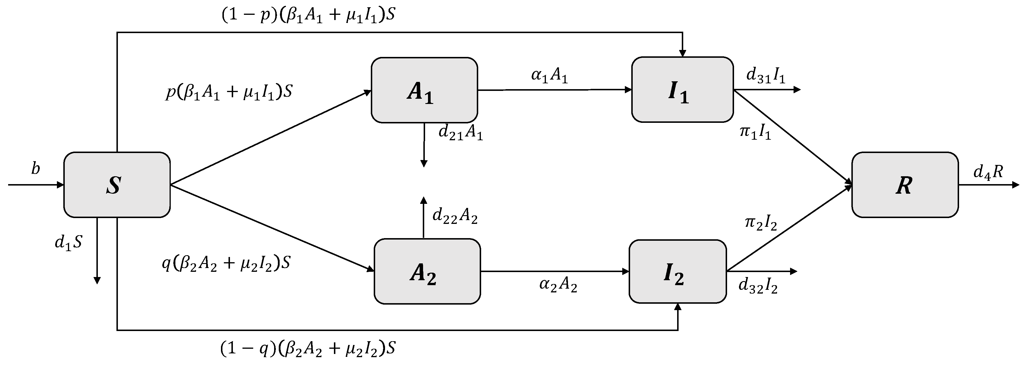
We consider a compartmental epidemic model describing the transmission dynamics of two competing pathogen strains in a homogeneous population. Let $N\left(t\right)$ denote the total population at time t. The population is divided into susceptible (S), asymptomatic infectious ($A_i$), symptomatic infectious ($I_i$), and recovered (R) compartments ($i=1,2$). Susceptible individuals become infected through effective contact with either asymptomatic or symptomatic infectious individuals carrying strain i. Upon infection, a proportion enters the asymptomatic class $A_i$, while the remainder progresses directly to the symptomatic class $I_i$. Individuals in the asymptomatic class may either develop symptoms or recover, whereas symptomatic individuals recover at strain-dependent rates. A schematic diagram of the model is shown in Figure 1.

Based on the above assumptions, the model is governed by the following system, where all parameters and their biological interpretations are summarized in

Table 1. Model parameters, descriptions, baseline values, and sources.

Parameter	Description	Value	Source
b	Recruitment rate of susceptible individuals	140	Assumed
${\beta }_1$	Transmission rate from asymptomatic individuals (strain 1)	$6.5\times {10}^{-5}$	Assumed
${\beta }_2$	Transmission rate from asymptomatic individuals (strain 2)	$6\times {10}^{-5}$	Assumed
${\mu }_1$	Transmission rate from symptomatic individuals (strain 1)	$4.3\times {10}^{-5}$	[31]
${\mu }_2$	Transmission rate from symptomatic individuals (strain 2)	$4\times {10}^{-5}$	[31]
p	Proportion entering asymptomatic class (strain 1)	$0.3$	[31]
q	Proportion entering asymptomatic class (strain 2)	$0.3$	[31]
${\alpha }_1$	Progression rate from $A_1$ to $I_1$	$0.2$	Assumed
${\alpha }_2$	Progression rate from $A_2$ to $I_2$	$0.2$	Assumed
${\pi }_1$	Recovery rate of symptomatic individuals (strain 1)	$0.75$	[31]
${\pi }_2$	Recovery rate of symptomatic individuals (strain 2)	$0.7$	Assumed
$d_1$	Natural death rate of susceptible individuals	$0.007$	Assumed
$d_{21}$	Natural death rate of asymptomatic individuals (strain 1)	$0.007$	Assumed
$d_{22}$	Natural death rate of asymptomatic individuals (strain 2)	$0.007$	Assumed
$d_{31}$	Natural death rate of symptomatic individuals (strain 1)	$0.007+7.79\times {10}^{-5}$	[32]
$d_{32}$	Natural death rate of symptomatic individuals (strain 2)	$0.007+7.79\times {10}^{-5}$	[32]
$d_4$	Natural death rate of recovered individuals	$0.007$	Assumed

.

$$\left\{\begin{array}{c}\begin{array}{c}{\displaystyle \frac{\mathrm{d}S}{\mathrm{d}t}}=b-({\beta }_1{A}_1+{\mu }_1{I}_1)S-({\beta }_2{A}_2+{\mu }_2{I}_2)S-d_{1}S,\hfill \\ {\displaystyle \frac{\mathrm{d}{A}_1}{\mathrm{d}t}}=p({\beta }_1{A}_1+{\mu }_1{I}_1)S-(d_{21}+{\alpha }_1)A_1,\hfill \\ {\displaystyle \frac{\mathrm{d}{I}_1}{\mathrm{d}t}}=(1-p)({\beta }_1{A}_1+{\mu }_1{I}_1)S+{\alpha }_1{A}_1-(d_{31}+{\pi }_1)I_1,\hfill \\ {\displaystyle \frac{\mathrm{d}{A}_2}{\mathrm{d}t}}=q({\beta }_2{A}_2+{\mu }_2{I}_2)S-(d_{22}+{\alpha }_2)A_2,\hfill \\ {\displaystyle \frac{\mathrm{d}{I}_2}{\mathrm{d}t}}=(1-q)({\beta }_2{A}_2+{\mu }_2{I}_2)S+{\alpha }_2{A}_2-(d_{32}+{\pi }_2)I_2,\hfill \\ {\displaystyle \frac{\mathrm{d}R}{\mathrm{d}t}}={\pi }_1{I}_1+{\pi }_2{I}_2-d_{4}R.\hfill \end{array}\hfill \end{array}\right.$$

(1)

Here, b denotes the recruitment rate of susceptible individuals. The parameters ${\beta }_i$ and ${\mu }_i$ represent the transmission rates associated with asymptomatic and symptomatic infectious individuals of strain i, respectively. The parameter ${\alpha }_i$ denotes the progression rate from $A_i$ to $I_i$, while ${\pi }_i$ is the recovery rate of symptomatic individuals. The parameters p and q denote the proportions of newly infected individuals who enter the asymptomatic class for strains 1 and 2, respectively. Natural death rates are denoted by $d_1$ for susceptibles, $d_{2i}$ for asymptomatic individuals, $d_{3i}$ for symptomatic individuals, and $d_4$ for recovered individuals.

2.2. Positivity of Solutions

We first show that all state variables of system (1) remain nonnegative.

Theorem 1.

For any nonnegative initial conditions

$$S\left(0\right),A_1\left(0\right),I_1\left(0\right),A_2\left(0\right),I_2\left(0\right),R\left(0\right)\ge 0,$$

the solution of system (1) satisfies

$$S\left(t\right),A_1\left(t\right),I_1\left(t\right),A_2\left(t\right),I_2\left(t\right),R\left(t\right)\ge 0,\forall t\ge 0.$$

Proof of Theorem 1. 

From the first equation of (1), we have ${\displaystyle \frac{\mathrm{d}S}{\mathrm{d}t}}=b-\Phi \left(t\right)S,$ where

$$\Phi \left(t\right)=({\beta }_1{A}_1+{\mu }_1{I}_1)+({\beta }_2{A}_2+{\mu }_2{I}_2)+d_1\ge 0.$$

By the comparison principle, it follows that $S\left(t\right)\ge 0$ for all $t\ge 0$.

Similarly, each of the remaining equations can be written in the form ${\displaystyle \frac{\mathrm{d}x}{\mathrm{d}t}}\ge -cx,$ for some $c>0$, which implies $x\left(t\right)\ge 0$ whenever $x\left(0\right)\ge 0$. Hence, all state variables remain nonnegative for all $t\ge 0$.    □

2.3. Invariant Region

Let $N\left(t\right)=S\left(t\right)+A_1\left(t\right)+A_2\left(t\right)+I_1\left(t\right)+I_2\left(t\right)+R\left(t\right)$ denote the total population. Summing all equations in (1), we obtain

$${\displaystyle \frac{\mathrm{d}N}{\mathrm{d}t}}=b-d_{1}S-d_{21}{A}_1-d_{31}{I}_1-d_{22}{A}_2-d_{32}{I}_2-d_{4}R\le b-\overline{d}N,$$

where $\overline{d}=min\{d_1,d_{21},d_{31},d_{22},d_{32},d_4\}.$ It follows that ${lim\; sup}_{t\to \infty }N\left(t\right)\le b/\overline{d}.$

Moreover, from the first equation of (1),

$${\displaystyle \frac{\mathrm{d}S}{\mathrm{d}t}}\le b-d_{1}S,$$

which yields

$$\underset{t\to \infty }{lim\; sup}S\left(t\right)\le {\displaystyle \frac{b}{d_1}}.$$

Since the recovered class R does not affect the first five equations, the dynamics can be reduced to the following subsystem:

$$\left\{\begin{array}{c}\begin{array}{cc}\hfill {\displaystyle \frac{\mathrm{d}S}{\mathrm{d}t}}& =b-({\beta }_1{A}_1+{\mu }_1{I}_1)S-({\beta }_2{A}_2+{\mu }_2{I}_2)S-d_{1}S,\hfill \\ \hfill {\displaystyle \frac{\mathrm{d}{A}_1}{\mathrm{d}t}}& =p({\beta }_1{A}_1+{\mu }_1{I}_1)S-(d_{21}+{\alpha }_1)A_1,\hfill \\ \hfill {\displaystyle \frac{\mathrm{d}{I}_1}{\mathrm{d}t}}& =(1-p)({\beta }_1{A}_1+{\mu }_1{I}_1)S+{\alpha }_1{A}_1-(d_{31}+{\pi }_1)I_1,\hfill \\ \hfill {\displaystyle \frac{\mathrm{d}{A}_2}{\mathrm{d}t}}& =q({\beta }_2{A}_2+{\mu }_2{I}_2)S-(d_{22}+{\alpha }_2)A_2,\hfill \\ \hfill {\displaystyle \frac{\mathrm{d}{I}_2}{\mathrm{d}t}}& =(1-q)({\beta }_2{A}_2+{\mu }_2{I}_2)S+{\alpha }_2{A}_2-(d_{32}+{\pi }_2)I_2.\hfill \end{array}\hfill \end{array}\right.$$

(2)

Therefore, the feasible region is defined as

$$\Gamma =\left\{(S,A_1,I_1,A_2,I_2)\in {\mathbb{R}}_{+}^5|S\le {\displaystyle \frac{b}{d_1}},N\le {\displaystyle \frac{b}{\overline{d}}}\right\}.$$

It is straightforward to verify that $\Gamma$ is positively invariant for system (2).

2.4. Equilibria and the Basic Reproduction Number

2.4.1. Disease-Free Equilibrium

System (2) always admits a unique disease-free equilibrium (DFE), denoted by $P_0$, located on the boundary of the feasible region $\Gamma$. It is given by

$$P_0=(S_0,0,0,0,0),\mathrm{with}{S}_0={\displaystyle \frac{b}{d_1}}.$$

2.4.2. Basic Reproduction Number

Following the next-generation matrix approach [33], we consider the infected state vector $X={(A_1,I_1,A_2,I_2)}^T.$ Let F and V denote the matrices of new infection terms and transition terms, respectively. Then, the basic reproduction number is given by ${\mathcal{R}}_0=\rho \left(F{V}^{-1}\right),$ where $\rho (·)$ denotes the spectral radius. Due to the block structure of the system, ${\mathcal{R}}_0$ can be decomposed as ${\mathcal{R}}_0=max\{{\mathcal{R}}_{01},{\mathcal{R}}_{02}\},$ where

$$\begin{array}{cc}\hfill {\mathcal{R}}_{01}& =\left[{\displaystyle \frac{p{\beta }_1}{d_{21}+{\alpha }_1}}+{\displaystyle \frac{p{\mu }_1{\alpha }_1}{(d_{31}+{\pi }_1)(d_{21}+{\alpha }_1)}}+{\displaystyle \frac{(1-p){\mu }_1}{d_{31}+{\pi }_1}}\right]{\displaystyle \frac{b}{d_1}},\hfill \\ \hfill {\mathcal{R}}_{02}& =\left[{\displaystyle \frac{q{\beta }_2}{d_{22}+{\alpha }_2}}+{\displaystyle \frac{q{\mu }_2{\alpha }_2}{(d_{32}+{\pi }_2)(d_{22}+{\alpha }_2)}}+{\displaystyle \frac{(1-q){\mu }_2}{d_{32}+{\pi }_2}}\right]{\displaystyle \frac{b}{d_1}}.\hfill \end{array}$$

Here, ${\mathcal{R}}_{01}$ and ${\mathcal{R}}_{02}$ correspond to the reproduction numbers of strain 1 (drug-sensitive) and strain 2 (drug-resistant), respectively.

2.4.3. Endemic Equilibria

Theorem 2.

The existence of endemic equilibria of system (2) is characterized as follows:

(i) 

If ${\mathcal{R}}_{01}>max\{1,{\mathcal{R}}_{02}\}$, then there exists a unique strain-1 endemic equilibrium

$$P_1^{*}=(S_1^{*},A_{11}^{*},I_{11}^{*},0,0).$$

(ii) 

If${\mathcal{R}}_{02}>max\{1,{\mathcal{R}}_{01}\}$, then there exists a unique strain-2 endemic equilibrium

$$P_2^{*}=(S_2^{*},0,0,A_{22}^{*},I_{22}^{*}).$$

(iii) 

If${\mathcal{R}}_{01}={\mathcal{R}}_{02}={\mathcal{R}}_0>1$, then system (2) admits a continuum of coexistence equilibria

$${\mathcal{E}}_{*}=\left\{P_3^{*}(S_3^{*},A_{13}^{*},I_{13}^{*},A_{23}^{*},I_{23}^{*}):\begin{array}{cc}& S_3^{*}={\displaystyle \frac{b}{d_1{\mathcal{R}}_0}},\hfill \\ & I_{13}^{*}={\displaystyle \frac{(1-p)(d_{21}+{\alpha }_1)+p{\alpha }_1}{p(d_{31}+{\pi }_1)}}{A}_{13}^{*},\hfill \\ & I_{23}^{*}={\displaystyle \frac{(1-q)(d_{22}+{\alpha }_2)+q{\alpha }_2}{q(d_{32}+{\pi }_2)}}{A}_{23}^{*},\hfill \\ & C_1{A}_{13}^{*}+C_2{A}_{23}^{*}=d_1({\mathcal{R}}_0-1),\hfill \\ & A_{13}^{*},A_{23}^{*}\ge 0\hfill \end{array}\right\}.$$

where

$$C_1={\beta }_1+{\mu }_1{\displaystyle \frac{(1-p)(d_{21}+{\alpha }_1)+p{\alpha }_1}{p(d_{31}+{\pi }_1)}},$$

and

$$C_2={\beta }_2+{\mu }_2{\displaystyle \frac{(1-q)(d_{22}+{\alpha }_2)+q{\alpha }_2}{q(d_{32}+{\pi }_2)}}.$$

Consequently, ${\mathcal{E}}_{*}$ forms a one-dimensional smooth manifold in the feasible region.

Proof of Theorem 2. 

(i) At the equilibrium $P_1^{*}$, all variables associated with strain 2 vanish. Solving the reduced subsystem yields

$$S_1^{*}={\displaystyle \frac{b}{d_1{\mathcal{R}}_{01}}},A_{11}^{*}={\displaystyle \frac{pb}{d_{21}+{\alpha }_1}}\left(1-{\displaystyle \frac{1}{{\mathcal{R}}_{01}}}\right),$$

$$I_{11}^{*}={\displaystyle \frac{\left((1-p)(d_{21}+{\alpha }_1)+p{\alpha }_1\right)b}{(d_{31}+{\pi }_1)(d_{21}+{\alpha }_1)}}\left(1-{\displaystyle \frac{1}{{\mathcal{R}}_{01}}}\right).$$

These quantities are positive if and only if ${\mathcal{R}}_{01}>1$. Moreover, the invasion reproduction number of strain 2 satisfies ${\mathcal{R}}_{02}<1$, which ensures that strain 2 cannot persist. Hence, the condition ${\mathcal{R}}_{01}>max\{1,{\mathcal{R}}_{02}\}$ guarantees the existence of $P_1^{*}$.

(ii) The existence of $P_2^{*}$ follows analogously by symmetry.

(iii) For coexistence equilibria, assume that both strains persist, namely $A_{13}^{*}>0,$$I_{13}^{*}>0,A_{23}^{*}>0,I_{23}^{*}>0.$ At equilibrium, from system (2), we obtain $S_3^{*}={\displaystyle \frac{b}{d_1{\mathcal{R}}_0}},$ where ${\mathcal{R}}_{01}={\mathcal{R}}_{02}={\mathcal{R}}_0>1.$ Moreover, the equilibrium relations imply

$$I_{13}^{*}={\displaystyle \frac{(1-p)(d_{21}+{\alpha }_1)+p{\alpha }_1}{p(d_{31}+{\pi }_1)}}{A}_{13}^{*},$$

and

$$I_{23}^{*}={\displaystyle \frac{(1-q)(d_{22}+{\alpha }_2)+q{\alpha }_2}{q(d_{32}+{\pi }_2)}}{A}_{23}^{*}.$$

Setting the right-hand sides of system (2) to zero leads to a linear system in $A_{13}^{*}$ and $A_{23}^{*}$:

$$\left\{\begin{array}{c}{d}_1({\mathcal{R}}_0-1)=C_1{A}_{13}^{*}+C_2{A}_{23}^{*},\hfill \\ b\left(1-{\displaystyle \frac{1}{{\mathcal{R}}_0}}\right)=D_1{A}_{13}^{*}+D_2{A}_{23}^{*},\hfill \end{array}\right.$$

where

$$C_1={\beta }_1+{\mu }_1{\displaystyle \frac{(1-p)(d_{21}+{\alpha }_1)+p{\alpha }_1}{p(d_{31}+{\pi }_1)}},C_2={\beta }_2+{\mu }_2{\displaystyle \frac{(1-q)(d_{22}+{\alpha }_2)+q{\alpha }_2}{q(d_{32}+{\pi }_2)}},$$

$$D_1={\displaystyle \frac{d_{21}+{\alpha }_1}{p}},D_2={\displaystyle \frac{d_{22}+{\alpha }_2}{q}}.$$

When ${\mathcal{R}}_{01}={\mathcal{R}}_{02}={\mathcal{R}}_0>1$, the coefficient matrix becomes singular with rank one. Therefore, the system admits infinitely many solutions, forming a one-dimensional continuum of equilibria.    □

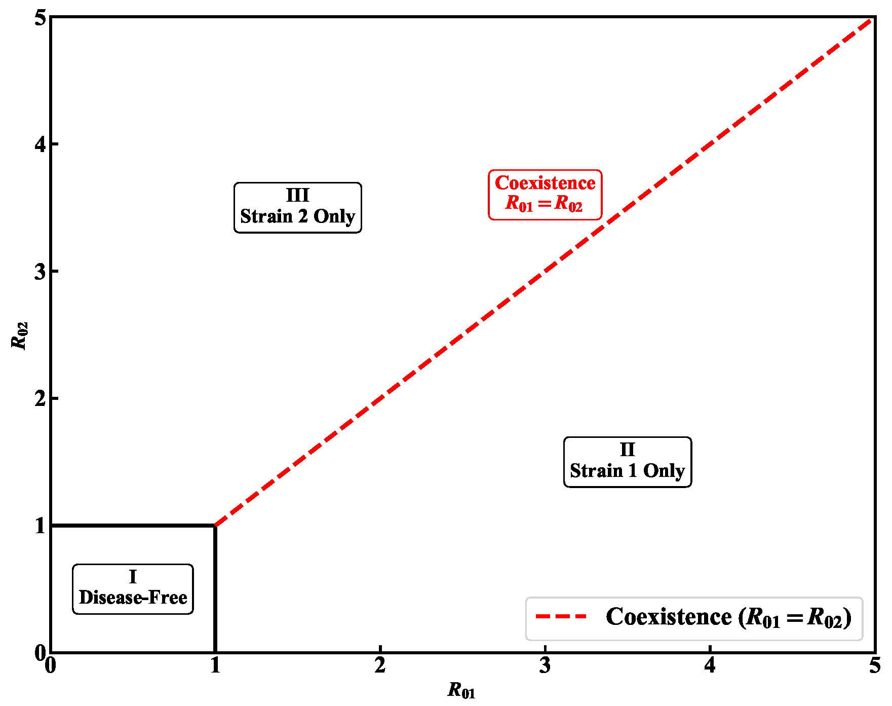
The qualitative dynamical structure in the $(R_{01},R_{02})$ parameter space is illustrated in Figure 2. In particular, competitive exclusion occurs when $R_{01}\ne R_{02}$, while the degenerate case $R_{01}=R_{02}=R_0>1$ gives rise to the continuum of equilibria.

3. Global Dynamical Analysis

3.1. Stability of the Disease-Free Equilibrium

We first investigate the stability of the disease-free equilibrium $P_0$.

Theorem 3.

If ${\mathcal{R}}_0<1$, then the disease-free equilibrium $P_0$ of system (2) is locally asymptotically stable in Γ. If ${\mathcal{R}}_0>1$, it is unstable.

Proof of Theorem 3. 

The Jacobian matrix of system (2) at $P_0$ is given by

$$J\left(P_0\right)=\left(\begin{array}{ccccc}-d_1& -{\beta }_1{S}_0& -{\mu }_1{S}_0& -{\beta }_2{S}_0& -{\mu }_2{S}_0\\ 0& p{\beta }_1{S}_0-{\widehat{d}}_1& p{\mu }_1{S}_0& 0& 0\\ 0& (1-p){\beta }_1{S}_0+{\alpha }_1& (1-p){\mu }_1{S}_0-{\widehat{d}}_2& 0& 0\\ 0& 0& 0& q{\beta }_2{S}_0-{\widehat{d}}_3& q{\mu }_2{S}_0\\ 0& 0& 0& (1-q){\beta }_2{S}_0+{\alpha }_2& (1-q){\mu }_2{S}_0-{\widehat{d}}_4\end{array}\right),$$

where ${\widehat{d}}_1=d_{21}+{\alpha }_1,{\widehat{d}}_2=d_{31}+{\pi }_1,{\widehat{d}}_3=d_{22}+{\alpha }_2,{\widehat{d}}_4=d_{32}+{\pi }_2.$ It is clear that one eigenvalue is ${\lambda }_1=-d_1<0$. The remaining eigenvalues are determined by two decoupled $2\times 2$ blocks corresponding to the two strains:

$$C=\left(\begin{array}{cc}p{\beta }_1{S}_0-{\widehat{d}}_1& p{\mu }_1{S}_0\\ (1-p){\beta }_1{S}_0+{\alpha }_1& (1-p){\mu }_1{S}_0-{\widehat{d}}_2\end{array}\right),D=\left(\begin{array}{cc}q{\beta }_2{S}_0-{\widehat{d}}_3& q{\mu }_2{S}_0\\ (1-q){\beta }_2{S}_0+{\alpha }_2& (1-q){\mu }_2{S}_0-{\widehat{d}}_4\end{array}\right).$$

   For matrix C, direct computation yields $det\left(C\right)={\widehat{d}}_1{\widehat{d}}_2(1-{\mathcal{R}}_{01}),tr\left(C\right)<0\mathrm{if}{\mathcal{R}}_{01}<1.$ Similarly, $det\left(D\right)={\widehat{d}}_3{\widehat{d}}_4(1-{\mathcal{R}}_{02}),tr\left(D\right)<0\mathrm{if}{\mathcal{R}}_{02}<1.$ Thus, all eigenvalues have negative real parts if and only if ${\mathcal{R}}_0=max\{{\mathcal{R}}_{01},{\mathcal{R}}_{02}\}<1.$ The result follows from the Hurwitz criterion.    □

Theorem 4.

If ${\mathcal{R}}_0<1$, then the disease-free equilibrium $P_0$ is globally asymptotically stable in Γ.

Proof of Theorem 4. 

Consider the Lyapunov function

$$L_0=a_1{A}_1+a_2{I}_1+a_3{A}_2+a_4{I}_2,$$

where

$$a_1={\displaystyle \frac{{\beta }_1}{d_{21}+{\alpha }_1}}+{\displaystyle \frac{{\mu }_1{\alpha }_1}{(d_{21}+{\alpha }_1)(d_{31}+{\pi }_1)}},a_2={\displaystyle \frac{{\mu }_1}{d_{31}+{\pi }_1}},$$

$$a_3={\displaystyle \frac{{\beta }_2}{d_{22}+{\alpha }_2}}+{\displaystyle \frac{{\mu }_2{\alpha }_2}{(d_{22}+{\alpha }_2)(d_{32}+{\pi }_2)}},a_4={\displaystyle \frac{{\mu }_2}{d_{32}+{\pi }_2}}.$$

   Differentiating $L_0$ along solutions gives

$${\displaystyle \frac{\mathrm{d}{L}_0}{\mathrm{d}t}}=({\beta }_1{A}_1+{\mu }_1{I}_1)\left({\displaystyle \frac{{\mathcal{R}}_{01}{d}_{1}S}{b}}-1\right)+({\beta }_2{A}_2+{\mu }_2{I}_2)\left({\displaystyle \frac{{\mathcal{R}}_{02}{d}_{1}S}{b}}-1\right).$$

Since $S\le {\displaystyle \frac{b}{d_1}}$ in $\Gamma$, it follows that ${\displaystyle \frac{\mathrm{d}{L}_0}{\mathrm{d}t}}\le 0$ whenever ${\mathcal{R}}_0<1$. Moreover, ${\displaystyle \frac{\mathrm{d}{L}_0}{\mathrm{d}t}}=0$ if and only if $A_1=I_1=A_2=I_2=0$. By LaSalle’s invariance principle, the solution converges to $P_0$. Hence, $P_0$ is globally asymptotically stable.    □

3.2. Stability of the Boundary Endemic Equilibrium

Theorem 5.

If ${\mathcal{R}}_{01}>max\{1,{\mathcal{R}}_{02}\}$, then the strain-1 endemic equilibrium $P_1^{*}$ is globally asymptotically stable in Γ.

Proof of Theorem 5. 

Consider the Lyapunov function

$$L_1=x_1\left(S-S_1^{*}ln{\displaystyle \frac{S}{S_1^{*}}}\right)+x_2\left(A_1-A_{11}^{*}ln{\displaystyle \frac{A_1}{A_{11}^{*}}}\right)+x_3\left(I_1-I_{11}^{*}ln{\displaystyle \frac{I_1}{I_{11}^{*}}}\right)+x_4{A}_2+x_5{I}_2,$$

where $x_i>0$$(i=1,\dots ,5)$. Differentiating $L_1$ along solutions of system (2), we obtain

$${\displaystyle \frac{\mathrm{d}{L}_1}{\mathrm{d}t}}=V_{11}+V_{12}+V_{13},$$

where

$$\begin{array}{cc}\hfill V_{11}& =d_1{S}_1^{*}\left(2-{\displaystyle \frac{S_1^{*}}{S}}-{\displaystyle \frac{S}{S_1^{*}}}\right)\le 0,\hfill \\ \hfill V_{12}& =-{\displaystyle \frac{S_1^{*2}}{S}}({\beta }_1{A}_{11}^{*}+{\mu }_1{I}_{11}^{*})-x_2{\displaystyle \frac{S}{A_1}}p{A}_{11}^{*}({\beta }_1{A}_1+{\mu }_1{I}_1)\hfill \\ \hfill & -x_3\left[{\displaystyle \frac{S}{I_1}}(1-p)I_{11}^{*}({\beta }_1{A}_1+{\mu }_1{I}_1)-{\displaystyle \frac{A_1}{I_1}}{I}_{11}^{*}{\alpha }_1\right],\hfill \\ \hfill V_{13}& =({\beta }_1{A}_{11}^{*}+{\mu }_1{I}_{11}^{*})S_1^{*}+x_2{A}_{11}^{*}(d_{21}+{\alpha }_1)+x_3(d_{31}+{\pi }_1)I_{11}^{*}.\hfill \end{array}$$

The coefficients $x_i$ are chosen such that

$$\left\{\begin{array}{c}-x_1+p{x}_2+(1-p)x_3=0,\hfill \\ -x_1+q{x}_4+(1-q)x_5=0,\hfill \\ x_1{\beta }_1{S}_1^{*}-x_2(d_{21}+{\alpha }_1)+x_3{\alpha }_1=0,\hfill \\ x_1{\mu }_1{S}_1^{*}-x_3(d_{31}+{\pi }_1)=0,\hfill \\ x_1{\beta }_2{S}_1^{*}-x_4(d_{22}+{\alpha }_2)+x_5{\alpha }_2=0,\hfill \\ x_1{\mu }_2{S}_1^{*}-x_5(d_{32}+{\pi }_2)=0.\hfill \end{array}\right.$$

(3)

A direct computation yields the positive solution

$$x_1=1,x_2={\displaystyle \frac{(d_{31}+{\pi }_1){\beta }_1{S}_1^{*}+{\mu }_1{\alpha }_1{S}_1^{*}}{(d_{31}+{\pi }_1)(d_{21}+{\alpha }_1)}},x_3={\displaystyle \frac{{\mu }_1{S}_1^{*}}{d_{31}+{\pi }_1}},$$

$$x_4={\displaystyle \frac{(d_{32}+{\pi }_2){\beta }_2{S}_1^{*}+{\mu }_2{\alpha }_2{S}_1^{*}}{(d_{32}+{\pi }_2)(d_{22}+{\alpha }_2)}},x_5={\displaystyle \frac{{\mu }_2{S}_1^{*}}{d_{32}+{\pi }_2}}.$$

Using the relation $-x_1+p{x}_2+(1-p)x_3=0$, the term $V_{12}$ can be rearranged as

$$\begin{array}{cc}\hfill V_{12}& =\left[-p{x}_2{\displaystyle \frac{S_1^{*2}}{S}}{\beta }_1{A}_{11}^{*}-x_{2}Sp{\beta }_1{A}_{11}^{*}\right]\hfill \\ & +\left[-(1-p)x_3{\displaystyle \frac{S_1^{*2}}{S}}{\mu }_1{I}_{11}^{*}-x_{3}S(1-p){\mu }_1{I}_{11}^{*}\right]\hfill \\ & +\left[-up{x}_2{\displaystyle \frac{S_1^{*2}}{S}}{\mu }_1{I}_{11}^{*}-u{x}_2{\displaystyle \frac{S{I}_1}{A_1}}p{\mu }_1{A}_{11}^{*}-x_3{\displaystyle \frac{A_1}{I_1}}{I}_{11}^{*}{\alpha }_1\right]\hfill \\ & +\left[-(1-p)x_3{\displaystyle \frac{S_1^{*2}}{S}}{\beta }_1{A}_{11}^{*}-x_3{\displaystyle \frac{S{A}_1}{I_1}}(1-p)I_{11}^{*}{\beta }_1\right]\hfill \\ & +\left[-(1-u)x_2{\displaystyle \frac{S{I}_1}{A_1}}p{\mu }_1{A}_{11}^{*}-(1-u)p{x}_2{\displaystyle \frac{S_1^{*2}}{S}}{\mu }_1{I}_{11}^{*}\right]\hfill \\ & \le -2x_{2}Sp{\beta }_1{A}_{11}^{*}-2x_{3}S(1-p){\mu }_1{I}_{11}^{*}-3{\left(u^2{p}^2{x}_2^2{x}_3{\mu }_1^2{I}_{11}^{*2}{A}_{11}^{*}{\alpha }_1{S}_1^{*2}\right)}^{1/3}\hfill \\ & -4{\left[{(1-u)}^2{p}^2{(1-p)}^2{x}_2^2{x}_3^2{\mu }_1^2{\beta }_1^2{I}_{11}^{*2}{A}_{11}^{*2}{S}_1^{*2}\right]}^{1/4},\hfill \end{array}$$

where

$$u={\displaystyle \frac{{\alpha }_1}{[(1-p)d_{21}+{\alpha }_1]x_2}},1-u={\displaystyle \frac{(1-p){\beta }_1{S}_1^{*}}{[(1-p)d_{21}+{\alpha }_1]x_2}}.$$

Similarly, we further obtain

$$V_{13}=2p{x}_2{\beta }_1{A}_{11}^{*}{S}_1^{*}+2(1-p)x_3{\mu }_1{I}_{11}^{*}{S}_1^{*}+3x_3{\alpha }_1{A}_{11}^{*}+4(1-p)x_3{\beta }_1{A}_{11}^{*}{S}_1^{*},$$

By the arithmetic mean–geometric mean inequality,

$$a_1+a_2+\dots +a_n\ge n{(a_1{a}_2\dots a_n)}^{1/n},a_i>0,$$

we obtain $V_{12}+V_{13}\le 0$. Therefore, ${\displaystyle \frac{\mathrm{d}{L}_1}{\mathrm{d}t}}\le 0\mathrm{in}\Gamma ,$ and equality holds if and only if $(S,A_1,I_1,A_2,I_2)=(S_1^{*},A_{11}^{*},I_{11}^{*},0,0).$ Hence, the largest invariant set contained in $\left\{x\in \Gamma :{\displaystyle \frac{\mathrm{d}{L}_1}{\mathrm{d}t}}=0\right\}$ is the singleton $\left\{P_1^{*}\right\}$. By LaSalle’s invariance principle, $P_1^{*}$ is globally asymptotically stable.    □

Theorem 6.

If ${\mathcal{R}}_{02}>max\{1,{\mathcal{R}}_{01}\}$, then the drug-resistant strain endemic equilibrium $P_2^{*}=(S_2^{*},0,0,A_{22}^{*},I_{22}^{*})$ is globally asymptotically stable in the feasible region Γ.

Proof of Theorem 6. 

Consider the Lyapunov function

$$L_2=x_1\left(S-S_2^{*}ln{\displaystyle \frac{S}{S_2^{*}}}\right)+x_6{A}_1+x_7{I}_1+x_8\left(A_2-A_{22}^{*}ln{\displaystyle \frac{A_2}{A_{22}^{*}}}\right)+x_9\left(I_2-I_{22}^{*}ln{\displaystyle \frac{I_2}{I_{22}^{*}}}\right),$$

where $x_i>0$. Differentiating $L_2$ along the solutions of system (2), we obtain

$${\displaystyle \frac{\mathrm{d}{L}_2}{\mathrm{d}t}}=V_{21}+V_{22}+V_{23},$$

where

$$\begin{array}{cc}\hfill V_{21}& =d_1{S}_2^{*}\left(2-{\displaystyle \frac{S_2^{*}}{S}}-{\displaystyle \frac{S}{S_2^{*}}}\right)\le 0,\hfill \\ \hfill V_{22}& =-{\displaystyle \frac{S_2^{*2}}{S}}({\beta }_2{A}_{22}^{*}+{\mu }_2{I}_{22}^{*})-x_8{\displaystyle \frac{S}{A_2}}q{A}_{22}^{*}({\beta }_2{A}_2+{\mu }_2{I}_2)\hfill \\ \hfill & -x_9\left[{\displaystyle \frac{S}{I_2}}(1-q)I_{22}^{*}({\beta }_2{A}_2+{\mu }_2{I}_2)-{\displaystyle \frac{A_2}{I_2}}{I}_{22}^{*}{\alpha }_2\right],\hfill \\ \hfill V_{23}& =({\beta }_2{A}_{22}^{*}+{\mu }_2{I}_{22}^{*})S_2^{*}+x_8{A}_{22}^{*}(d_{22}+{\alpha }_2)+x_9(d_{32}+{\pi }_2)I_{22}^{*}.\hfill \end{array}$$

The coefficients are chosen such that

$$\left\{\begin{array}{c}-x_1+p{x}_6+(1-p)x_7=0,\hfill \\ -x_1+q{x}_8+(1-q)x_9=0,\hfill \\ x_1{\beta }_1{S}_2^{*}-x_6(d_{21}+{\alpha }_1)+x_7{\alpha }_1=0,\hfill \\ x_1{\mu }_1{S}_2^{*}-x_7(d_{31}+{\pi }_1)=0,\hfill \\ x_1{\beta }_2{S}_2^{*}-x_8(d_{22}+{\alpha }_2)+x_9{\alpha }_2=0,\hfill \\ x_1{\mu }_2{S}_2^{*}-x_9(d_{32}+{\pi }_2)=0.\hfill \end{array}\right.$$

(4)

A direct computation gives

$$x_6={\displaystyle \frac{(d_{31}+{\pi }_1){\beta }_1{S}_2^{*}+{\mu }_1{\alpha }_1{S}_2^{*}}{(d_{31}+{\pi }_1)(d_{21}+{\alpha }_1)}},x_7={\displaystyle \frac{{\mu }_1{S}_2^{*}}{d_{31}+{\pi }_1}},$$

$$x_8={\displaystyle \frac{(d_{32}+{\pi }_2){\beta }_2{S}_2^{*}+{\mu }_2{\alpha }_2{S}_2^{*}}{(d_{32}+{\pi }_2)(d_{22}+{\alpha }_2)}},x_9={\displaystyle \frac{{\mu }_2{S}_2^{*}}{d_{32}+{\pi }_2}}.$$

Using the relation $q{x}_8+(1-q)x_9=x_1$, the term $V_{22}$ can be rewritten as

$$\begin{array}{cc}\hfill V_{22}& =\left[-q{x}_8{\displaystyle \frac{S_2^{*2}}{S}}{\beta }_2{A}_{22}^{*}-x_{8}Sq{\beta }_2{A}_{22}^{*}\right]+\left[-(1-q)x_9{\displaystyle \frac{S_2^{*2}}{S}}{\mu }_2{I}_{22}^{*}-x_{9}S(1-q){\mu }_2{I}_{22}^{*}\right]\hfill \\ \hfill & +\left[-u^{*}q{x}_8{\displaystyle \frac{S_2^{*2}}{S}}{\mu }_2{I}_{22}^{*}-u^{*}{x}_8{\displaystyle \frac{S{I}_2}{A_2}}q{\mu }_2{A}_{22}^{*}-x_9{\displaystyle \frac{A_2}{I_2}}{I}_{22}^{*}{\alpha }_2\right]\hfill \\ \hfill & +\left[-(1-q)x_9{\displaystyle \frac{S_2^{*2}}{S}}{\beta }_2{A}_{22}^{*}-x_9{\displaystyle \frac{S{A}_2}{I_2}}(1-q)I_{22}^{*}{\beta }_2\right]\hfill \\ \hfill & +\left[-(1-u^{*})x_8{\displaystyle \frac{S{I}_2}{A_2}}p{\mu }_2{A}_{22}^{*}-(1-u^{*})q{x}_8{\displaystyle \frac{S_2^{*2}}{S}}{\mu }_2{I}_{22}^{*}\right]\hfill \\ \hfill & \le -2x_{8}Sq{\beta }_2{A}_{22}^{*}-2x_{9}S(1-q){\mu }_2{I}_{22}^{*}-3{\left(u^{*2}{q}^2{x}_8^2{x}_9{\mu }_2^2{I}_{22}^{*2}{A}_{22}^{*}{\alpha }_2{S}_2^{*2}\right)}^{1/3}\hfill \\ \hfill & -4{\left[{(1-u^{*})}^2{q}^2{(1-q)}^2{x}_6^2{x}_9^2{\mu }_2^3{\beta }_2^2{I}_{22}^{*2}{A}_{22}^{*2}{S}_2^{*2}\right]}^{1/4},\hfill \end{array}$$

where

$$u^{*}={\displaystyle \frac{{\alpha }_2}{\left[(1-q)d_{22}+{\alpha }_2\right]x_8}},1-u^{*}={\displaystyle \frac{(1-q){\beta }_2{S}_2^{*}}{\left[(1-q)d_{22}+{\alpha }_2\right]x_8}}.$$

Similarly, using the balance relations (4), $V_{23}$ can be further simplified as

$$V_{23}=2q{x}_8{\beta }_2{A}_{22}^{*}{S}_2^{*}+2(1-q)x_9{\mu }_2{I}_{22}^{*}{S}_2^{*}+3x_9{\alpha }_2{A}_{22}^{*}+4(1-q)x_9{\beta }_2{A}_{22}^{*}{S}_2^{*}.$$

Consequently, we obtain $V_{22}+V_{23}\le 0,$ which implies ${\displaystyle \frac{\mathrm{d}{L}_2}{\mathrm{d}t}}\le 0\mathrm{in}\Gamma .$ Moreover, ${\displaystyle \frac{\mathrm{d}{L}_2}{\mathrm{d}t}}=0$ if and only if $(S,A_1,I_1,A_2,I_2)=(S_2^{*},0,0,A_{22}^{*},I_{22}^{*}).$ Therefore, the largest invariant set contained in $\left\{x\in \Gamma :{\displaystyle \frac{\mathrm{d}{L}_2}{\mathrm{d}t}}=0\right\}$ is the singleton $\left\{P_2^{*}\right\}$. By LaSalle’s invariance principle, $P_2^{*}$ is globally asymptotically stable.    □

3.3. Stability of the Coexistence Equilibrium Set

In this subsection, we analyze the local stability of the coexistence endemic equilibrium set of system (2). The analysis relies on center manifold theory due to the presence of a zero eigenvalue.

3.3.1. Preliminary Lemmas

We first recall several classical results from invariant manifold theory.

Lemma 1

([34]). Consider the dynamical system

$${\displaystyle \frac{\mathrm{d}x}{\mathrm{d}t}}=f\left(x\right),x\in {\mathbb{R}}^n,$$

where f is sufficiently smooth and $f\left(0\right)=0$. Let ${\lambda }_1,\dots ,{\lambda }_n$ be the eigenvalues of the Jacobian matrix $J=Df\left(0\right)$. Define

$${\sigma }_s=\{{\lambda }_i:Re\left({\lambda }_i\right)<0\},{\sigma }_u=\{{\lambda }_i:Re\left({\lambda }_i\right)>0\},{\sigma }_c=\{{\lambda }_i:Re\left({\lambda }_i\right)=0\}.$$

Then there exist locally invariant manifolds tangent to the corresponding eigenspaces, namely the stable manifold $W^s$, unstable manifold $W^u$, and center manifold $W^c$.

Lemma 2

([35]). Consider the system

$$\left\{\begin{array}{c}{\displaystyle \frac{\mathrm{d}x}{\mathrm{d}t}}=Ax+f(x,y),x\in T^c,\hfill \\ {\displaystyle \frac{\mathrm{d}y}{\mathrm{d}t}}=By+g(x,y),y\in T^s,\hfill \end{array}\right.$$

where $f(0,0)=0$, $g(0,0)=0$, and $Df(0,0)=Dg(0,0)=0$. Then there exists a locally invariant center manifold $W^c$ tangent to $T^c$ at the origin, which can be expressed as

$$W^c=\{(x,y)\in T^c\times T^s:y=h\left(x\right)\},$$

where $h\left(0\right)=0$ and $Dh\left(0\right)=0$. Moreover, the dynamics restricted to the center manifold are governed by the reduced system

$${\displaystyle \frac{\mathrm{d}u}{\mathrm{d}t}}=Au+f(u,h\left(u\right)),u\in T^c.$$

Lemma 3

([34]). Let $T^{su}$ denote the $(n-1)$-dimensional eigenspace associated with all nonzero eigenvalues of J. Then $y\in T^{su}$ if and only if

$$\langle l,y\rangle =0,$$

where l is the left eigenvector corresponding to the zero eigenvalue of J.

3.3.2. Jacobian Matrix and Spectral Structure

Let $P_3^{*}$ be a coexistence equilibrium with ${\mathcal{R}}_{01}={\mathcal{R}}_{02}={\mathcal{R}}_0>1$. Denote

$$t_3={\beta }_1{A}_{13}^{*}+{\mu }_1{I}_{13}^{*},t_4={\beta }_2{A}_{23}^{*}+{\mu }_2{I}_{23}^{*}.$$

The Jacobian matrix $J\left(P_3^{*}\right)$ is given by

$$J\left(P_3^{*}\right)=\left(\begin{array}{ccccc}-d_1{\mathcal{R}}_0& -{\beta }_1{S}^{*}& -{\mu }_1{S}^{*}& -{\beta }_2{S}^{*}& -{\mu }_2{S}^{*}\\ p{t}_3& p{\beta }_1{S}^{*}-{\widehat{d}}_1& p{\mu }_{1}S*& 0& 0\\ (1-p)t_3& (1-p)1S*+{\alpha }_1& (1-p){\mu }_{1}S*-{\widehat{d}}_2& 0& 0\\ q{t}_4& 0& 0& q{\beta }_{2}S*-{\widehat{d}}_3& q{\mu }_{2}S*\\ (1-q)t_4& 0& 0& J_{54}^{*}& J_{55}^{*}\end{array}\right).$$

where

$$J_{54}^{*}=(1-q){\beta }_{2}S*+{\alpha }_2, J_{55}^{*}=(1-q){\mu }_{2}S*-{\widehat{d}}_4.$$

A direct computation shows that the characteristic polynomial can be factorized as

$$\det (\lambda I-J(P_3^{*}\left)\right)=\lambda P_2\left(\lambda \right) Q_2\left(\lambda \right),$$

where

$$P_2\left(\lambda \right)={\lambda }^2+a_1\lambda +a_2, Q_2\left(\lambda \right)={\lambda }^2+b_1\lambda +b_2,$$

with coefficients

$$\begin{array}{cc}& a_1={\widehat{d}}_1+{\widehat{d}}_2-S^{*}\left(p{\beta }_1+(1-p){\mu }_1\right),\hfill \\ & a_2={\widehat{d}}_1{\widehat{d}}_2-S^{*}\left({\widehat{d}}_{2}p{\beta }_1+{\widehat{d}}_1(1-p){\mu }_1\right),\hfill \\ & b_1={\widehat{d}}_3+{\widehat{d}}_4-S^{*}\left(q{\beta }_2+(1-q){\mu }_2\right),\hfill \\ & b_2={\widehat{d}}_3{\widehat{d}}_4-S^{*}\left({\widehat{d}}_{4}q{\beta }_2+{\widehat{d}}_3(1-q){\mu }_2\right).\hfill \end{array}$$

It follows immediately that $\lambda =0$ is an eigenvalue of $J\left(P_3^{*}\right)$. Moreover, under the condition ${\mathcal{R}}_{01}={\mathcal{R}}_{02}={\mathcal{R}}_0>1$, the coexistence equilibrium satisfies $S^{*}={\displaystyle \frac{b}{d_1{\mathcal{R}}_0}}$. Using the definition of ${\mathcal{R}}_{01}$ we obtain

$$1=S^{*}\left[{\displaystyle \frac{p{\beta }_1}{{\widehat{d}}_1}}+{\displaystyle \frac{p{\mu }_1{\alpha }_1}{{\widehat{d}}_1{\widehat{d}}_2}}+{\displaystyle \frac{(1-p){\mu }_1}{{\widehat{d}}_2}}\right].$$

Multiplying both sides by ${\widehat{d}}_1{\widehat{d}}_2$ gives

$${\widehat{d}}_1{\widehat{d}}_2=S^{*}\left({\widehat{d}}_{2}p{\beta }_1+p{\mu }_1{\alpha }_1+{\widehat{d}}_1(1-p){\mu }_1\right).$$

Hence, $a_2={\widehat{d}}_1{\widehat{d}}_2-S^{*}\left({\widehat{d}}_{2}p{\beta }_1+{\widehat{d}}_1(1-p){\mu }_1\right)=S^{*}p{\mu }_1{\alpha }_1>0$.

Next, we verify the positivity of $a_1$. Since

$${\widehat{d}}_1{\widehat{d}}_2=S^{*}\left({\widehat{d}}_{2}p{\beta }_1+p{\mu }_1{\alpha }_1+{\widehat{d}}_1(1-p){\mu }_1\right)>S^{*}\left({\widehat{d}}_{2}p{\beta }_1+{\widehat{d}}_1(1-p){\mu }_1\right).$$

Dividing both sides by ${\hat{d}}_1$>0 yields

$$1>S^{*}\left({\displaystyle \frac{p{\beta }_1}{{\widehat{d}}_1}}+{\displaystyle \frac{(1-p){\mu }_1}{{\widehat{d}}_2}}\right).$$

Since

$${\displaystyle \frac{1}{{\widehat{d}}_1}}>{\displaystyle \frac{1}{{\widehat{d}}_1+{\widehat{d}}_2}},{\displaystyle \frac{1}{{\widehat{d}}_2}}>{\displaystyle \frac{1}{{\widehat{d}}_1+{\widehat{d}}_2}},$$

we further obtain

$$1>S^{*}{\displaystyle \frac{p{\beta }_1+(1-p){\mu }_1}{{\widehat{d}}_1+{\widehat{d}}_2}},$$

which implies $S*(p{\beta }_1+(1-p\left){\mu }_1\right)<{\widehat{d}}_1+{\widehat{d}}_2$.

Similarly, one can prove that $b_1>0,b_2>0.$ Therefore, by the Routh–Hurwitz criterion, all roots of $P_2\left(\lambda \right)=0$ and $Q_2\left(\lambda \right)=0$ have strictly negative real parts. Consequently, the Jacobian matrix $J\left(P_3^{*}\right)$ admits a simple zero eigenvalue, while all remaining eigenvalues lie in the open left half-plane.

Hence, the coexistence equilibrium $P_3^{*}$ is non-hyperbolic with a one-dimensional center subspace and a four-dimensional stable subspace.

3.3.3. Main Result

Theorem 7.

If $R_{01}=R_{02}=R_0>1$, then the coexistence endemic equilibrium $P_3^{*}$ of System (2) is locally stable in the feasible region Γ.

Proof of Theorem 7. 

Step 1.

Center manifold reduction

Let $x={(S,A_1,I_1,A_2,I_2)}^T$ and denote by $x^{*}$ the coexistence equilibrium. Let $J\left(x^{*}\right)$ be the Jacobian matrix at $x^{*}$. Under the condition $R_{01}=R_{02}=R_0>1$, it follows from Lemmas 1 and 2 that $J\left(x^{*}\right)$ admits a simple zero eigenvalue, while all other eigenvalues have strictly negative real parts. Hence, there exists a one-dimensional center manifold $W^c$ in a neighborhood of $x^{*}$,which can be expressed as

$$W^c\left(x^{*}\right)=\left\{(x,y)\in T^c\times T^s:y=\omega \left(x\right),|x-x^{*}|<\delta ,\omega \left(x^{*}\right)=x^{*},D\omega \left(x^{*}\right)=0\right\},$$

Let r and l be the right and left eigenvectors associated with the zero eigenvalue of $J\left(x^{*}\right)$, respectively.

The right eigenvector r is obtained from $J\left(x^{*}\right)r=0$. Choosing $r_1=0$ and normalizing by $r_2=1$, we obtain

$$r={\left(0,1,{\displaystyle \frac{(1-p)d_{21}+{\alpha }_1}{p({\pi }_1+d_{31})}},-{\displaystyle \frac{q(d_{21}+{\alpha }_1)}{p(d_{22}+{\alpha }_2)}},-{\displaystyle \frac{(d_{21}+{\alpha }_1)}{p(d_{22}+{\alpha }_2)}}·{\displaystyle \frac{(1-q)d_{22}+{\alpha }_2}{{\pi }_2+d_{32}}}\right)}^T.$$

The left eigenvector l is determined by $l^{T}J\left(x^{*}\right)=0$. Choosing $l_1=0$ and $l_2=1$, we obtain $l={(0,1,l_3,l_4,l_5)}^T,$ where

$$l_3={\displaystyle \frac{p{\beta }_1{S}_3^{*}-{\widehat{d}}_1}{(1-p){\beta }_1{S}_3^{*}+{\alpha }_1}},l_4=-{\displaystyle \frac{\left[p+(1-p)l_3\right]t_3}{\left[q+(1-q){\displaystyle \frac{q{\beta }_2{S}_3^{*}-{\widehat{d}}_3}{(1-q){\beta }_2{S}_3^{*}+{\alpha }_2}}\right]t_4}},l_5=l_3·l_4.$$

Then, let $c=l^{T}r\ne 0$. According to Lemma 3, the deviation of the state variable from the equilibrium can be decomposed as

$$x=x^{*}+{\displaystyle \frac{1}{c}}ur+\omega \left(u\right).$$

Here, $u=l^T(x-x^{*})$ represents the projection of $(x-x^{*})$ onto the critical direction, while $ur\in T^c$, $\omega \left(u\right)\in T^s$, and the function $\omega \left(u\right)$ satisfies $\omega \left(0\right)=0$, $D\omega \left(0\right)=0$. Thus, the pair $(u,\omega (u\left)\right)$ defines a local coordinate system in a neighborhood of $x^{*}$.

Since $\omega \left(u\right)$ can be expanded around $u=0$ as $\omega \left(u\right)=h_2{u}^2+h_3{u}^3+O\left(u^4\right)$, by Lemma 2, the dynamics of System (2) restricted to the center manifold are governed by the reduced scalar equation

$${\displaystyle \frac{\mathrm{d}u}{\mathrm{d}t}}=l^T{\displaystyle \frac{\mathrm{d}x}{\mathrm{d}t}}.$$

Step 2.

Derivation of the reduced equation

We now determine the dynamics of the reduced system. To this end, we expand the vector field $f\left(x\right)$ in a neighborhood of $x^{*}$:

$${\displaystyle \frac{\mathrm{d}x}{\mathrm{d}t}}=f\left(x\right)=f\left(x^{*}\right)+J\left(x^{*}\right)(x-x^{*})+G\left(x\right)=J\left(x^{*}\right)(x-x^{*})+G\left(x\right),$$

where $G\left(x\right)$ collects all higher-order nonlinear terms and satisfies

$$G\left(x\right)={\left({\displaystyle \frac{\mathrm{d}S}{\mathrm{d}t}},{\displaystyle \frac{\mathrm{d}{A}_1}{\mathrm{d}t}},{\displaystyle \frac{\mathrm{d}{I}_1}{\mathrm{d}t}},{\displaystyle \frac{\mathrm{d}{A}_2}{\mathrm{d}t}},{\displaystyle \frac{\mathrm{d}{I}_2}{\mathrm{d}t}}\right)}^T-J\left(x^{*}\right){\left(S-S^{*},A_1-A_{13}^{*},I_1-I_{13}^{*},A_2-A_{23}^{*},I_2-I_{23}^{*}\right)}^T,$$

By Taylor expansion, we have

$$G\left(x\right)=G\left(x^{*}\right)+DG\left(x^{*}\right)(x-x^{*})+{\displaystyle \frac{1}{2}}{(x-x^{*})}^{T}H(x-x^{*}).$$

Since $G\left(x^{*}\right)=DG\left(x^{*}\right)=0$, it follows that $G\left(x\right)={\displaystyle \frac{1}{2}}{(x-x^{*})}^{T}H(x-x^{*}).$ Here $H={(H_1,H_2,H_3,H_4,H_5)}^T$, where

$$H_1=\left(\begin{array}{ccccc}0& -{\beta }_1& -{\mu }_1& -{\beta }_2& -{\mu }_2\\ -{\beta }_1& 0& 0& 0& 0\\ -{\mu }_1& 0& 0& 0& 0\\ -{\beta }_2& 0& 0& 0& 0\\ -{\mu }_2& 0& 0& 0& 0\end{array}\right),H_2=\left(\begin{array}{ccccc}0& p{\beta }_1& p{\mu }_1& 0& 0\\ p{\beta }_1& 0& 0& 0& 0\\ p{\mu }_1& 0& 0& 0& 0\\ 0& 0& 0& 0& 0\\ 0& 0& 0& 0& 0\end{array}\right),$$

$$H_3=\left(\begin{array}{ccccc}0& (1-p){\beta }_1& (1-p){\mu }_1& 0& 0\\ (1-p){\beta }_1& 0& 0& 0& 0\\ (1-p){\mu }_1& 0& 0& 0& 0\\ 0& 0& 0& 0& 0\\ 0& 0& 0& 0& 0\end{array}\right),H_4=\left(\begin{array}{ccccc}0& 0& 0& q{\beta }_2& q{\mu }_2\\ 0& 0& 0& 0& 0\\ 0& 0& 0& 0& 0\\ q{\beta }_2& 0& 0& 0& 0\\ q{\mu }_2& 0& 0& 0& 0\end{array}\right),$$

$$H_5=\left(\begin{array}{ccccc}0& 0& 0& (1-q){\beta }_2& (1-q){\mu }_2\\ 0& 0& 0& 0& 0\\ 0& 0& 0& 0& 0\\ (1-q){\beta }_2& 0& 0& 0& 0\\ (1-q){\mu }_2& 0& 0& 0& 0\end{array}\right).$$

Define $B:{\mathbb{R}}^5\times {\mathbb{R}}^5\to {\mathbb{R}}^5$. Given two vectors $a,b\in {\mathbb{R}}^5$, the output is a vector $B(a,b)\in {\mathbb{R}}^5$. Its i-th component is given by $B{(a,b)}_i={\sum }_{j=1}^5{\sum }_{k=1}^5{H}_{ijk}{a}_j{b}_k$, where $H_{ijk}$ are the components of the Hessian tensor. Substituting $x=x^{*}+ur+\omega \left(u\right)$ into the above equation yields

$$G\left(x^{*}+{\displaystyle \frac{1}{c}}ur+\omega \left(u\right)\right)={\displaystyle \frac{1}{c}}{u}^{3}B(r,h_2)+u^4\left[{\displaystyle \frac{1}{c}}B(r,h_3)+{\displaystyle \frac{1}{2}}B(h_2,h_2)\right]+O\left(u^4\right),$$

Thus, the reduced system becomes

$$\begin{array}{cc}\hfill {\displaystyle \frac{\mathrm{d}u}{\mathrm{d}t}}& =l^T\left[J\left(x^{*}\right)\left({\displaystyle \frac{1}{c}}ur+\omega \left(u\right)\right)+G\left(x^{*}+{\displaystyle \frac{1}{c}}ur+\omega \left(u\right)\right)\right]\hfill \\ \hfill & =l^T\left[{\displaystyle \frac{1}{c}}{u}^{3}B(r,h_2)+u^4\left({\displaystyle \frac{1}{c}}B(r,h_3)+{\displaystyle \frac{1}{2}}B(h_2,h_2)\right)+O\left(u^4\right)\right].\hfill \end{array}$$

Step 3.

Stability analysis

From $x=x^{*}+{\displaystyle \frac{1}{c}}ur+\omega \left(u\right)$, $u=l^T(x-x^{*})$, we obtain

$${\displaystyle \frac{\mathrm{d}x}{\mathrm{d}t}}=f\left(x\right)={\displaystyle \frac{1}{c}}{\displaystyle \frac{\mathrm{d}u}{\mathrm{d}t}}r+{\displaystyle \frac{\mathrm{d}\omega }{\mathrm{d}t}}={\displaystyle \frac{1}{c}}{l}^T{\displaystyle \frac{\mathrm{d}x}{\mathrm{d}t}}r+{\displaystyle \frac{\mathrm{d}\omega }{\mathrm{d}t}}={\displaystyle \frac{1}{c}}{l}^{T}f\left(x\right)r+{\displaystyle \frac{\mathrm{d}\omega }{\mathrm{d}t}},$$

which further yields

$$\begin{array}{cc}\hfill {\displaystyle \frac{\mathrm{d}\omega }{\mathrm{d}t}}& =\left(I-{\displaystyle \frac{r{l}^T}{c}}\right)f\left(x\right)\hfill \\ \hfill & =\left(I-{\displaystyle \frac{r{l}^T}{c}}\right)\left[J\left(x^{*}\right)\left({\displaystyle \frac{1}{c}}ur+\omega \left(u\right)\right)+G\left(x^{*}+{\displaystyle \frac{1}{c}}ur+\omega \left(u\right)\right)\right]\hfill \\ \hfill & =J\left(x^{*}\right)\omega \left(u\right)+\left(I-{\displaystyle \frac{r{l}^T}{c}}\right)\left[{\displaystyle \frac{1}{c}}{u}^3(r,h_2)+u^4\left({\displaystyle \frac{1}{c}}B(r,h_3)+{\displaystyle \frac{1}{2}}B(h_2,h_2)\right)+O\left(u^4\right)\right],\hfill \end{array}$$

Since $\omega \left(u\right)=h_2{u}^2+h_3{u}^3+O\left(u^4\right)$, we have

$$\begin{array}{cc}\hfill {\displaystyle \frac{\mathrm{d}\omega }{\mathrm{d}t}}& ={\displaystyle \frac{\mathrm{d}\omega }{\mathrm{d}u}}{\displaystyle \frac{\mathrm{d}u}{\mathrm{d}t}}\hfill \\ \hfill & =(2h_{2}u+3h_3{u}^2+O\left(u^3\right))l^T\left[{\displaystyle \frac{1}{c}}{u}^{3}B(r,h_2)+u^4\left({\displaystyle \frac{1}{c}}B(r,h_3)+{\displaystyle \frac{1}{2}}B(h_2,h_2)\right)+O\left(u^4\right)\right].\hfill \end{array}$$

Then, we obtain $h_2=0$. By recursively applying the same procedure to higher-order terms, we further obtain $h_3=0,h_4=0$ and so on. Consequently, all higher-order coefficients vanish, leading to ${\displaystyle \frac{\mathrm{d}u}{\mathrm{d}t}}=0$ on the center manifold. Hence, every point on the center manifold is an equilibrium, the center direction is neutrally stable, and the stability of the original system is determined solely by the stable eigenvalues, which are all negative. Therefore, the coexistence endemic equilibrium is locally stable.    □

Theorem 8.

If $R_{01}=R_{02}=R_0>1$, then the coexistence endemic equilibrium is globally attractive in Γ.

Proof of Theorem 8. 

We construct the following Volterra-type Lyapunov function

$$\begin{array}{cc}\hfill L& =x_1\left(S-S_3^{*}ln{\displaystyle \frac{S}{S_3^{*}}}\right)+\widehat{x_2}\left(A_1-A_{13}^{*}ln{\displaystyle \frac{A_1}{A_{13}^{*}}}\right)+\widehat{x_3}\left(I_1-I_{13}^{*}ln{\displaystyle \frac{I_1}{I_{13}^{*}}}\right)\hfill \\ \hfill & +\widehat{x_8}\left(A_2-A_{23}^{*}ln{\displaystyle \frac{A_2}{A_{23}^{*}}}\right)+\widehat{x_9}\left(I_2-I_{23}^{*}ln{\displaystyle \frac{I_2}{I_{23}^{*}}}\right),\hfill \end{array}$$

where $x_1,{\widehat{x}}_2,{\widehat{x}}_3,{\widehat{x}}_8,{\widehat{x}}_9>0$ are constants to be determined. Differentiating $L\left(t\right)$ along the trajectories of system (2) yields

$$\begin{array}{cc}\hfill {\displaystyle \frac{\mathrm{d}L}{\mathrm{d}t}}& =x_1\left[d_1{S}_3^{*}\left(2-{\displaystyle \frac{S_3^{*}}{S}}-{\displaystyle \frac{S}{S_3^{*}}}\right)+({\beta }_1{A}_{13}^{*}+{\mu }_1{I}_{13}^{*})\left(S_3^{*}-{\displaystyle \frac{S_3^{*2}}{S}}\right)+({\beta }_2{A}_{23}^{*}+{\mu }_2{I}_{23}^{*})\left(S_3^{*}-{\displaystyle \frac{S_3^{*2}}{S}}\right)\right]\hfill \\ \hfill & +\widehat{x_2}\left[A_{13}^{*}(d_{21}+{\alpha }_1)-{\displaystyle \frac{S}{A_1}}p{A}_{13}^{*}({\beta }_1{A}_1+{\mu }_1{I}_1)\right]\hfill \\ \hfill & +\widehat{x_3}\left[(d_{31}+{\pi }_1)I_{13}^{*}-{\displaystyle \frac{S}{I_1}}(1-p)I_{13}^{*}({\beta }_1{A}_1+{\mu }_1{I}_1)-{\displaystyle \frac{A_1}{I_1}}{I}_{13}^{*}{\alpha }_1\right]\hfill \\ \hfill & +\widehat{x_8}\left[A_{23}^{*}(d_{22}+{\alpha }_2)-{\displaystyle \frac{S}{A_2}}q{A}_{23}^{*}({\beta }_2{A}_2+{\mu }_2{I}_2)\right]\hfill \\ \hfill & +\widehat{x_9}\left[(d_{32}+{\pi }_2)I_{23}^{*}-{\displaystyle \frac{S}{I_2}}(1-q)I_{23}^{*}({\beta }_2{A}_2+{\mu }_2{I}_2)-{\displaystyle \frac{A_2}{I_2}}{I}_{23}^{*}{\alpha }_2\right],\hfill \end{array}$$

where the above equality holds under the condition

$$\left\{\begin{array}{c}-x_1+p\widehat{x_2}+(1-p)\widehat{x_3}=0,\hfill \\ -x_1+q\widehat{x_8}+(1-q)\widehat{x_9}=0,\hfill \\ x_1{\beta }_1{S}_3^{*}-\widehat{x_2}(d_{21}+{\alpha }_1)+\widehat{x_3}{\alpha }_1=0,\hfill \\ x_1{\mu }_1{S}_3^{*}-\widehat{x_3}(d_{31}+{\pi }_1)=0,\hfill \\ x_1{\beta }_2{S}_3^{*}-\widehat{x_8}(d_{23}+{\alpha }_2)+\widehat{x_9}{\alpha }_2=0,\hfill \\ x_1{\mu }_2{S}_3^{*}-\widehat{x_9}({\pi }_2+d_{32})=0.\hfill \end{array}\right.$$

(5)

We choose the positive constants $\widehat{x_2},\widehat{x_3},\widehat{x_8},\widehat{x_9}$ as

$$\widehat{x_2}={\displaystyle \frac{(d_{31}+{\pi }_1){\beta }_1{S}_3^{*}+{\mu }_1{\alpha }_1{S}_3^{*}}{(d_{31}+{\pi }_1)(d_{21}+{\alpha }_1)}},\widehat{x_3}={\displaystyle \frac{{\mu }_1{S}_3^{*}}{(d_{31}+{\pi }_1)}},$$

$$\widehat{x_8}={\displaystyle \frac{(d_{32}+{\pi }_2){\beta }_2{S}_3^{*}+{\mu }_2{\alpha }_2{S}_3^{*}}{(d_{32}+{\pi }_2)(d_{22}+{\alpha }_2)}},\widehat{x_9}={\displaystyle \frac{{\mu }_2{S}_3^{*}}{(d_{32}+{\pi }_2)}}.$$

Therefore, ${\displaystyle \frac{\mathrm{d}L}{\mathrm{d}t}}$ can be rewritten as ${\displaystyle \frac{\mathrm{d}L}{\mathrm{d}t}}=V_1+V_2+V_3+V_4+V_5$, where

$$\begin{array}{cc}\hfill V_1& =d_1{S}_3^{*}\left(2-{\displaystyle \frac{S_3^{*}}{S}}-{\displaystyle \frac{S}{S_3^{*}}}\right)\le 0,\hfill \\ \hfill V_2& =-{\displaystyle \frac{S_3^{*2}}{S}}({\beta }_1{A}_{13}^{*}+{\mu }_1{I}_{13}^{*})-\widehat{x_2}{\displaystyle \frac{S}{A_1}}p{A}_{13}^{*}({\beta }_1{A}_1+{\mu }_1{I}_1)\hfill \\ \hfill & -\widehat{x_3}\left[{\displaystyle \frac{S}{I_1}}(1-p)I_{13}^{*}({\beta }_1{A}_1+{\mu }_1{I}_1)-{\displaystyle \frac{A_1}{I_1}}{I}_{13}^{*}{\alpha }_1\right],\hfill \\ \hfill V_3& =({\beta }_1{A}_{13}^{*}+{\mu }_1{I}_{13}^{*})S_3^{*}+\widehat{x_2}{A}_{13}^{*}(d_{21}+{\alpha }_1)+\widehat{x_3}(d_{31}+{\pi }_1)I_{13}^{*},\hfill \\ \hfill V_4& =-{\displaystyle \frac{S_3^{*2}}{S}}({\beta }_2{A}_{23}^{*}+{\mu }_2{I}_{23}^{*})-\widehat{x_8}{\displaystyle \frac{S}{A_2}}q{A}_{23}^{*}({\beta }_2{A}_2+{\mu }_2{I}_2)\hfill \\ \hfill & -\widehat{x_9}\left[{\displaystyle \frac{S}{I_2}}(1-q)I_{23}^{*}({\beta }_2{A}_2+{\mu }_2{I}_2)-{\displaystyle \frac{A_2}{I_2}}{I}_{23}^{*}{\alpha }_2\right],\hfill \\ \hfill V_5& =({\beta }_2{A}_{23}^{*}+{\mu }_2{I}_{23}^{*})S_3^{*}+\widehat{x_8}{A}_{23}^{*}(d_{22}+{\alpha }_2)+\widehat{x_9}(d_{32}+{\pi }_2)I_{23}^{*}.\hfill \end{array}$$

For $V_2$, using $p\widehat{x_2}+(1-p)\widehat{x_3}=x_1$, we can rewrite it as

$$\begin{array}{cc}\hfill V_2& =\left[-p\widehat{x_2}{\displaystyle \frac{S_3^{*2}}{S}}{\beta }_1{A}_{13}^{*}-\widehat{x_2}Sp{\beta }_1{A}_{13}^{*}\right]+\left[-(1-p)\widehat{x_3}{\displaystyle \frac{S_3^{*2}}{S}}{\mu }_1{I}_{13}^{*}-\widehat{x_2}S(1-p){\mu }_1{I}_{13}^{*}\right]\hfill \\ \hfill & +\left[-u_{1}p\widehat{x_2}{\displaystyle \frac{S_3^{*2}}{S}}{\mu }_1{I}_{13}^{*}-u_1\widehat{x_2}{\displaystyle \frac{S{I}_1}{A_1}}p{\mu }_1{A}_{13}^{*}-\widehat{x_3}{\displaystyle \frac{A_1}{I_1}}{I}_{13}^{*}{\alpha }_1\right]\hfill \\ \hfill & +\left[-(1-p)\widehat{x_3}{\displaystyle \frac{S_3^{*2}}{S}}{\beta }_1{A}_{13}^{*}-\widehat{x_3}{\displaystyle \frac{S{A}_1}{I_1}}(1-p)I_{13}^{*}{\beta }_1\right]\hfill \\ \hfill & +\left[-(1-u_1)\widehat{x_2}{\displaystyle \frac{S{I}_1}{A_1}}p{\mu }_1{A}_{13}^{*}-(1-u_1)p\widehat{x_2}{\displaystyle \frac{S_3^{*2}}{S}}{\mu }_1{I}_{13}^{*}\right]\hfill \\ \hfill & \le -2\widehat{x_2}Sp{\beta }_1{A}_{13}^{*}-2\widehat{x_3}S(1-p){\mu }_1{I}_{13}^{*}-3{\left(u_1^2{p}^2{\widehat{x_2}}^2\widehat{x_3}{\mu }_1^2{I}_{13}^{*2}{A}_{13}^{*}{\alpha }_1{S}_3^{*2}\right)}^{1/3}\hfill \\ \hfill & -4{\left[{(1-u_1)}^2{p}^2{(1-p)}^2{\widehat{x_2}}^2{\widehat{x_3}}^2{\mu }_1^2{\beta }_1^2{I}_{13}^{*2}{A}_{13}^{*2}{S}_3^{*2}\right]}^{1/4},\hfill \end{array}$$

where

$$u_1={\displaystyle \frac{{\alpha }_1}{[(1-p)d_{21}+{\alpha }_1]\widehat{x_2}}},1-u_1={\displaystyle \frac{(1-p){\beta }_1{S}_3^{*}}{[(1-p)d_{21}+{\alpha }_1]\widehat{x_2}}}.$$

For $V_4$, using $q\widehat{x_8}+(1-q)\widehat{x_9}=x_1$, we obtain

$$\begin{array}{cc}\hfill V_4& =\left[-q\widehat{x_8}{\displaystyle \frac{S_3^{*2}}{S}}{\beta }_2{A}_{23}^{*}-\widehat{x_8}Sq{\beta }_2{A}_{23}^{*}\right]+\left[-(1-q)\widehat{x_9}{\displaystyle \frac{S_3^{*2}}{S}}{\mu }_2{I}_{23}^{*}-\widehat{x_8}S(1-q){\mu }_2{I}_{23}^{*}\right]\hfill \\ \hfill & +\left[-u_{2}q\widehat{x_8}{\displaystyle \frac{S_3^{*2}}{S}}{\mu }_2{I}_{23}^{*}-u_2\widehat{x_8}{\displaystyle \frac{S{I}_2}{A_2}}q{\mu }_2{A}_{23}^{*}-\widehat{x_9}{\displaystyle \frac{A_2}{I_2}}{I}_{23}^{*}{\alpha }_2\right]\hfill \\ \hfill & +\left[-(1-q)\widehat{x_9}{\displaystyle \frac{S_3^{*2}}{S}}{\beta }_2{A}_{23}^{*}-\widehat{x_9}{\displaystyle \frac{S{A}_2}{I_2}}(1-q)I_{23}^{*}{\beta }_2\right]\hfill \\ \hfill & +\left[-(1-u_2)\widehat{x_8}{\displaystyle \frac{S{I}_2}{A_2}}p{\mu }_2{A}_{23}^{*}-(1-u_2)q\widehat{x_8}{\displaystyle \frac{S_3^{*2}}{S}}{\mu }_2{I}_{23}^{*}\right]\hfill \\ \hfill & \le -2\widehat{x_8}Sq{\beta }_2{A}_{23}^{*}-2\widehat{x_9}S(1-q){\mu }_2{I}_{23}^{*}-3{\left(u_2^2{q}^2{\widehat{x_8}}^2\widehat{x_9}{\mu }_2^2{I}_{23}^{*2}{A}_{23}^{*}{\alpha }_2{S}_3^{*2}\right)}^{1/3}\hfill \\ \hfill & -4{\left[{(1-u_2)}^2{q}^2{(1-q)}^2{\widehat{x_8}}^2{\widehat{x_9}}^2{\mu }_2^2{\beta }_2^2{I}_{23}^{*2}{A}_{23}^{*2}{S}_3^{*2}\right]}^{1/4},\hfill \end{array}$$

where

$$u_2={\displaystyle \frac{{\alpha }_2}{[(1-p)d_{22}+{\alpha }_2]\widehat{x_8}}},1-u_2={\displaystyle \frac{(1-q){\beta }_2{S}_3^{*}}{[(1-p)d_{22}+{\alpha }_2]\widehat{x_8}}}.$$

Using relations (5), $V_3$ can be further expressed as

$$V_3=2p\widehat{x_2}{\beta }_1{A}_{13}^{*}{S}_3^{*}+2(1-p)\widehat{x_3}{\mu }_1{I}_{13}^{*}{S}_3^{*}+3\widehat{x_3}{\alpha }_1{A}_{13}^{*}+4(1-p)\widehat{x_3}{\beta }_1{A}_{13}^{*}{S}_3^{*},$$

Similarly, we can rewrite $V_5$ as

$$V_5=2q\widehat{x_8}{\beta }_2{A}_{23}^{*}{S}_3^{*}+2(1-q)\widehat{x_9}{\mu }_2{I}_{23}^{*}{S}_3^{*}+3\widehat{x_9}{\alpha }_2{A}_{23}^{*}+4(1-q)\widehat{x_9}{\beta }_2{A}_{23}^{*}{S}_3^{*},$$

by the arithmetic mean–geometric mean inequality, we derive $V_2+V_4\le 0$, $V_3+V_5\le 0$.

Combining the above results, we obtain ${\displaystyle \frac{\mathrm{d}L}{\mathrm{d}t}}\le 0$, and equality holds if and only if $(S_3^{*},A_{13}^{*},I_{13}^{*},A_{23}^{*},I_{23}^{*})$ belongs to the set of coexistence endemic equilibria in the feasible domain $\Gamma$. Therefore, by the Lyapunov function method, we conclude that all solutions of system (2) converge to the set of coexistence endemic equilibria, i.e., the system is globally stable in $\Gamma$.    □

4. Sensitivity Analysis

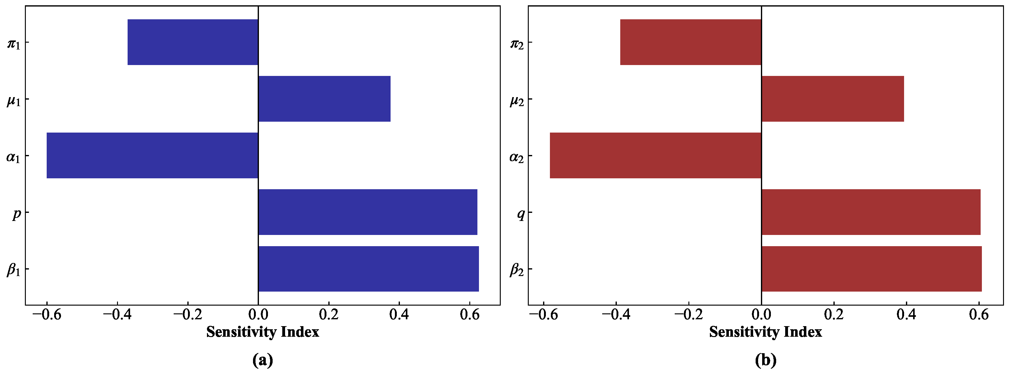
In this section, a global sensitivity analysis is performed using the Partial Rank Correlation Coefficient (PRCC) method combined with Latin Hypercube Sampling (LHS), with $R_{01}$ and $R_{02}$ as outputs. As illustrated in Figure 3, the parameters ${\mu }_1$, ${\beta }_1$, and p exhibit a strong positive correlation with $R_{01}$, while ${\pi }_1$ and ${\alpha }_1$ are negatively correlated with $R_{01}$. Similarly, ${\mu }_2$, ${\beta }_2$, and q show significant positive correlations with $R_{02}$, whereas ${\pi }_2$ and ${\alpha }_2$ are negatively correlated with $R_{02}$. These results provide important insights for disease control. In particular, reducing transmission rates or increasing recovery rates can effectively suppress disease spread by shortening the infectious period and lowering the overall transmission potential. The consistency of these effects across both strains highlights the robustness of the proposed control strategies.

5. Numerical Simulations

In this section, numerical simulations are performed to illustrate and complement the theoretical results obtained in the previous sections. In particular, the simulations are used to demonstrate the global dynamical behavior of System (2) under different threshold conditions, including convergence toward the disease-free equilibrium, single-strain endemic equilibria, and the coexistence equilibrium manifold arising in the degenerate case. All simulations in this section are carried out numerically using Python (3.14). The system of ordinary differential equations is solved with the solve_ivp function from the scipy.integrate package.

The parameter values used in the simulations are listed in Table 1. Some parameters are adopted from the existing literature whenever available, while the remaining ones are chosen for illustrative purposes in the absence of reliable epidemiological data. It should be emphasized that the main theoretical results of this paper, including the existence of equilibria, stability properties, and the continuum of coexistence equilibria, are established analytically and do not depend on any specific parameter choice. Different parameter values may affect the quantitative behavior of the solutions, but the qualitative dynamical properties remain valid provided the corresponding threshold conditions are satisfied.

Moreover, the numerical examples are intended to visualize the distinct asymptotic behaviors predicted by the analysis and to highlight the role of parameter degeneracy in generating a continuum of coexistence equilibria, which cannot be observed in classical epidemic models with isolated endemic states.

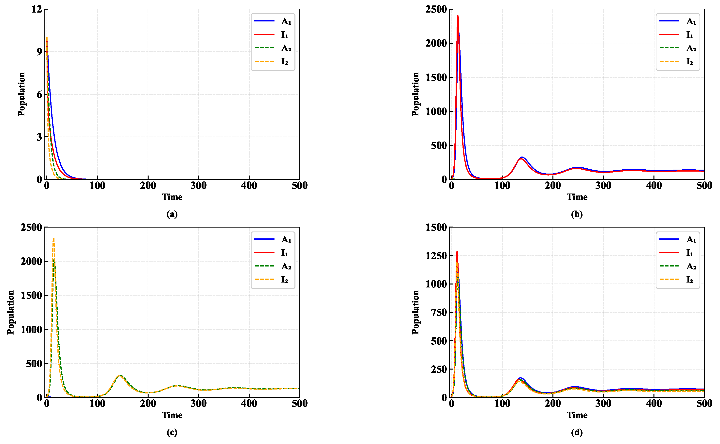
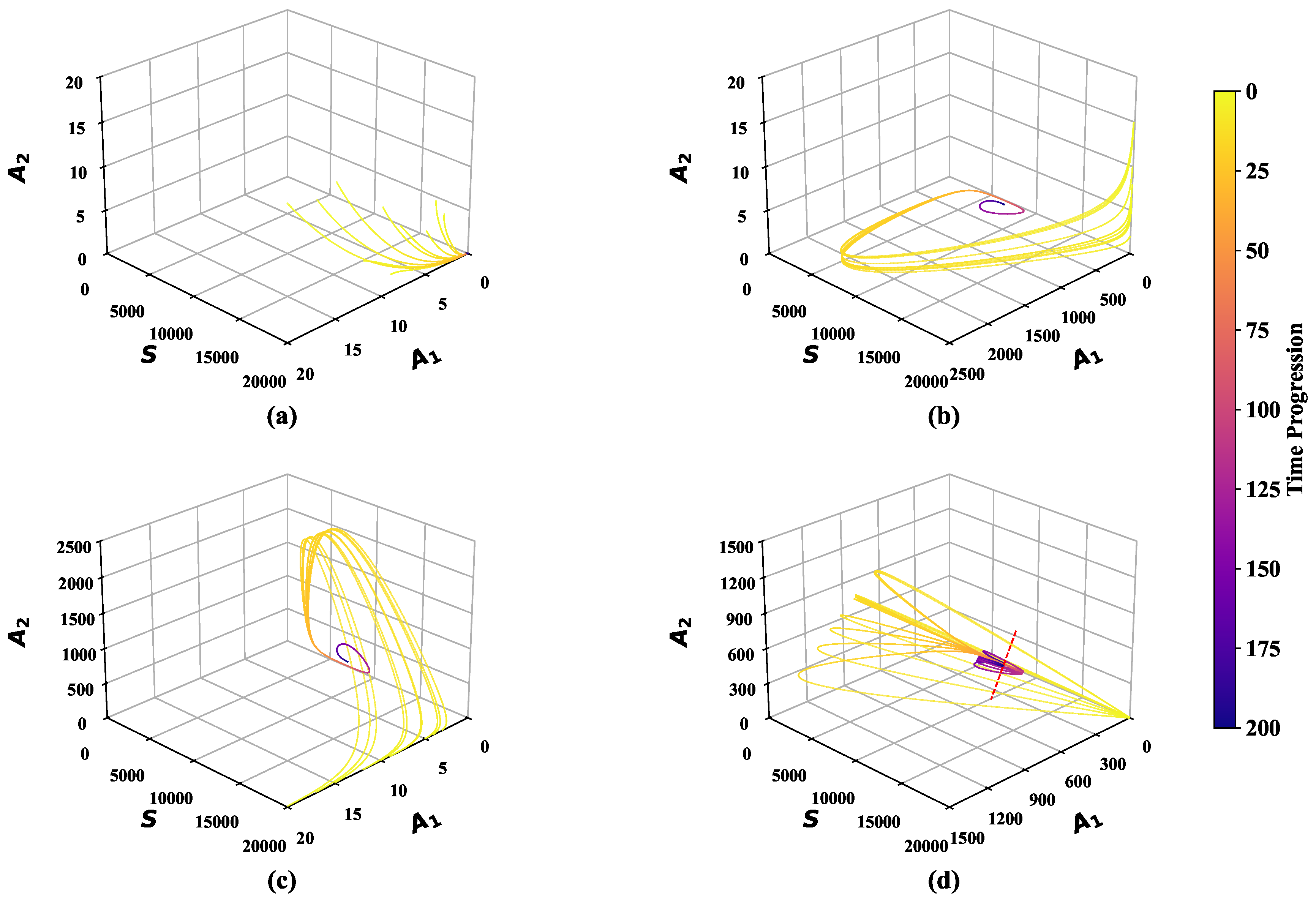
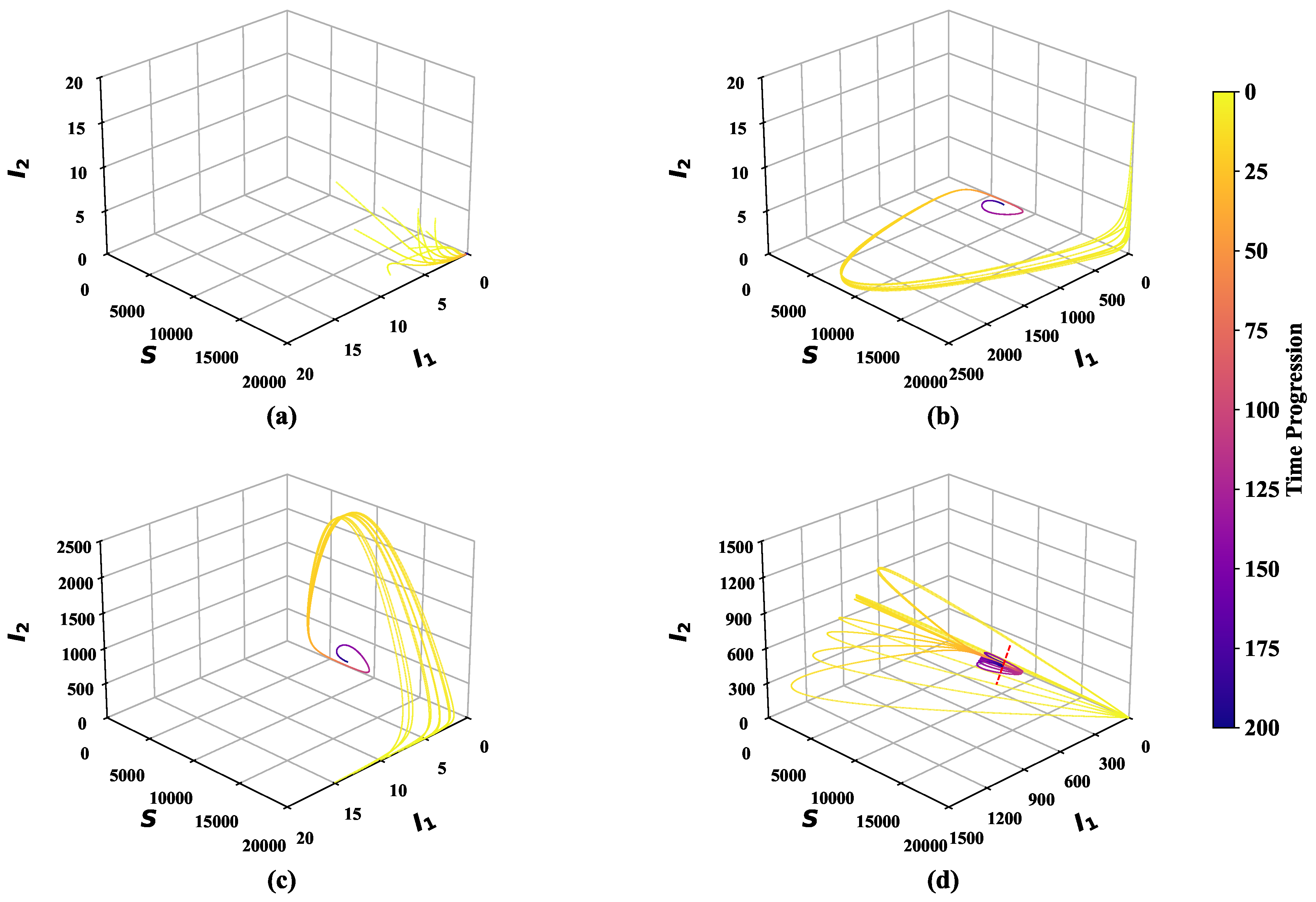
Figure 4 illustrates the global dynamics under different parameter regimes. The system converges to the disease-free equilibrium when $R_{01}<1$ and $R_{02}<1$, to a boundary equilibrium when one strain dominates, and to a coexistence equilibrium when $R_{01}=R_{02}>1$. To further illustrate the global dynamics, three-dimensional phase portraits are constructed in the $(A_1,A_2,S)$ and $(I_1,I_2,S)$ spaces (see Figure 5 and Figure 6). The numerical results are consistent with the theoretical analysis: solutions converge to the disease-free equilibrium when $R_0<1$, and to a unique boundary endemic equilibrium when one strain dominates the other. In particular, when $R_{01}=R_{02}>1$, trajectories converge to different equilibrium points lying on a one-dimensional manifold, providing numerical evidence for the existence of a continuum of endemic equilibria.

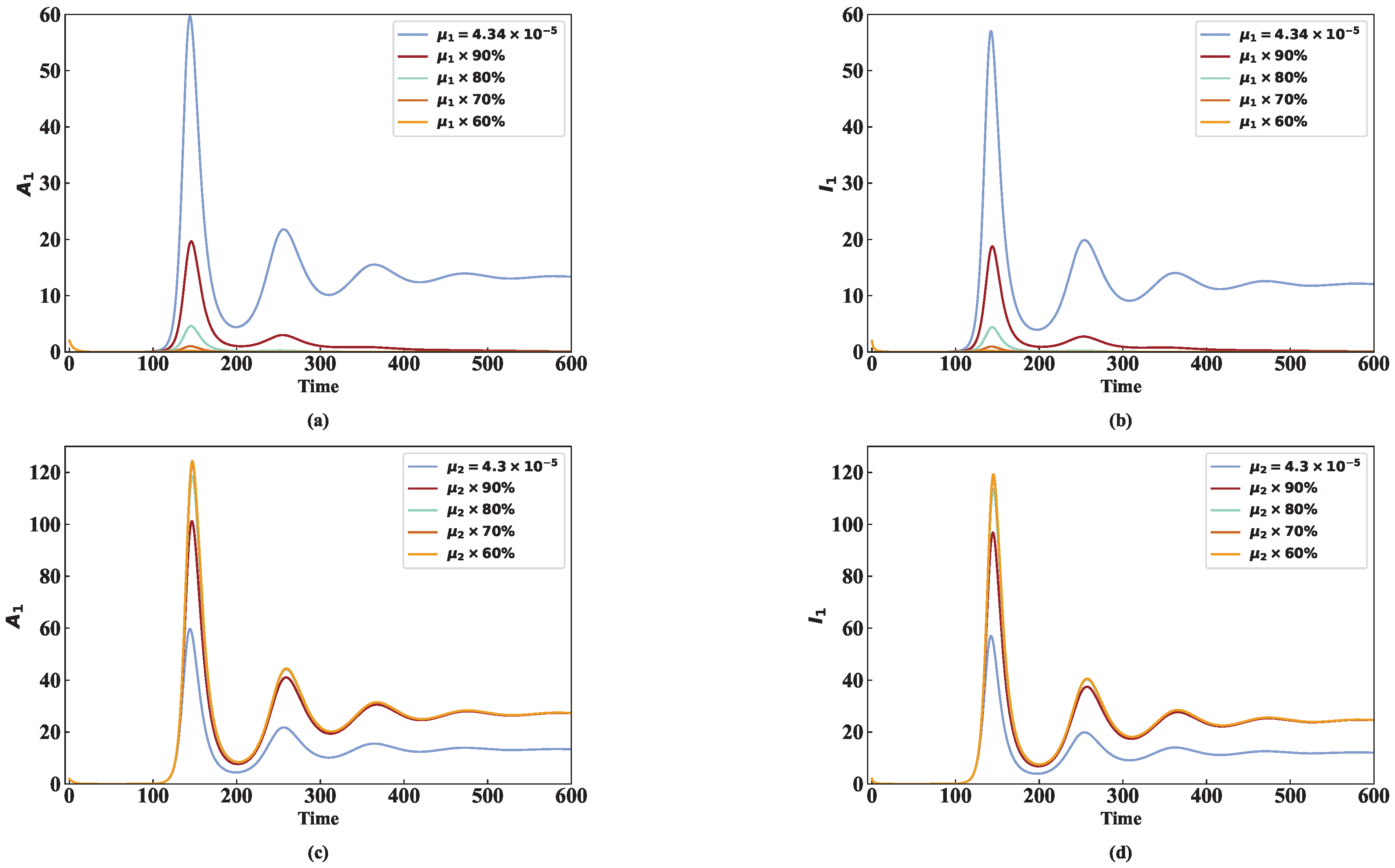
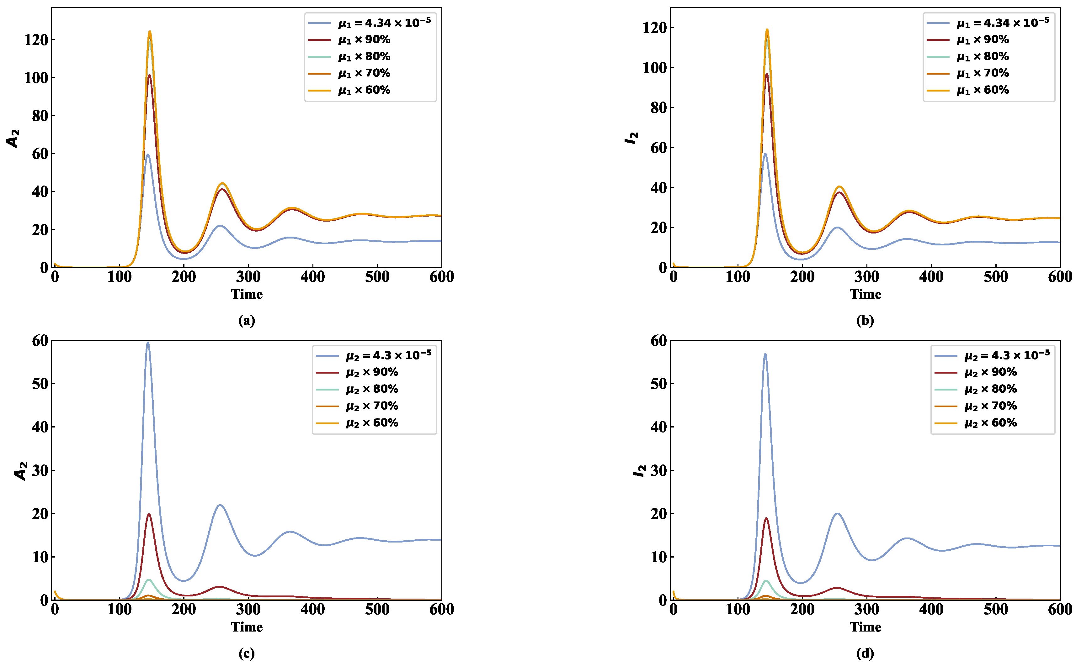
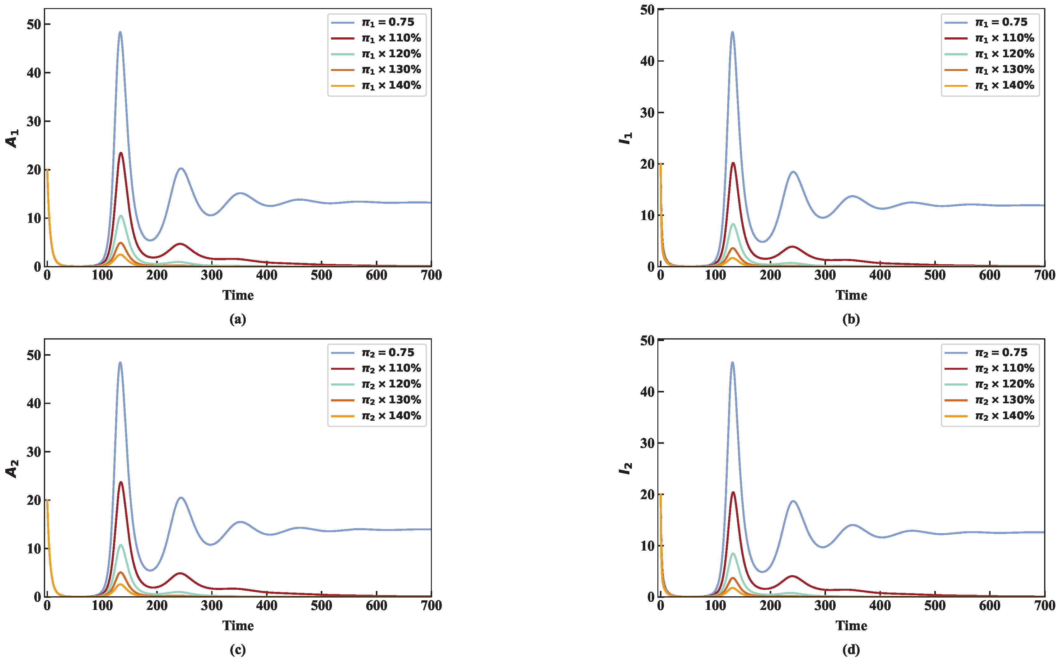
To examine the influence of key parameters, simulations are conducted for transmission, recovery, and transition rates (Figure 7, Figure 8, Figure 9 and Figure 10). As shown in Figure 7, decreasing ${\mu }_1$ leads to a substantial reduction in both asymptomatic and symptomatic populations of the drug-sensitive strain, accompanied by a delayed outbreak and a lower endemic level. In contrast, decreasing ${\mu }_2$ weakens the competitive pressure imposed by the drug-resistant strain, resulting in an increase in the prevalence of the sensitive strain. Similarly, a reduction in ${\mu }_2$ significantly suppresses the infection levels of the resistant strain, while decreasing ${\mu }_1$ promotes its persistence due to reduced competition from the sensitive strain. These results highlight that the relative transmission advantages between strains play a decisive role in determining competitive outcomes.

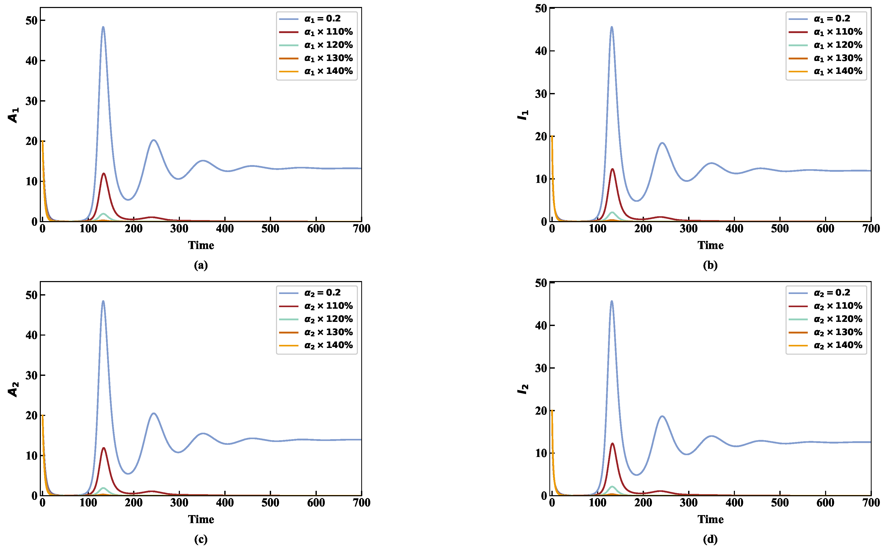
Figure 9 shows that increasing the recovery rates ${\pi }_1$ and ${\pi }_2$ reduces infection levels and lowers endemic equilibria, thereby shortening the infectious period. However, asymmetry in recovery rates may shift the competitive balance between strains. Figure 10 illustrates the effects of transition (screening) rates ${\alpha }_1$ and ${\alpha }_2$. Higher transition rates reduce the asymptomatic population and influence the distribution between asymptomatic and symptomatic classes, thereby affecting overall transmission dynamics. This suggests that enhanced screening and early detection are crucial for controlling diseases with significant asymptomatic transmission.

Overall, the numerical simulations reveal that transmission rates primarily determine strain dominance, recovery rates regulate infection persistence, and transition rates control hidden transmission pathways. These findings provide important insights into the design of effective intervention strategies for multi-strain infectious diseases.

6. Discussion

This study develops and analyzes a two-strain SAIR epidemic model with asymptomatic transmission and reveals a degenerate dynamical structure characterized by a continuum of endemic equilibria. This feature departs from the classical framework of isolated equilibria in multi-strain epidemic models.

The results show that the basic reproduction numbers ${\mathcal{R}}_{01}$ and ${\mathcal{R}}_{02}$ determine the global dynamics. When ${\mathcal{R}}_{01}\ne {\mathcal{R}}_{02}$, the system exhibits competitive exclusion, with the strain of larger reproduction number dominating. When ${\mathcal{R}}_{01}={\mathcal{R}}_{02}>1$, the system admits a continuum of coexistence equilibria forming a one-dimensional manifold. These equilibria are non-hyperbolic and possess neutral stability along a center direction. By combining Lyapunov methods with center manifold analysis, the equilibrium set is shown to be globally attractive.

From an epidemiological perspective, this degenerate structure corresponds to a regime of neutral competition, where competing strains have identical transmission potential. In this case, the long-term distribution of strains depends on initial conditions rather than parameter differences. This mechanism provides a possible explanation for the coexistence of pathogen variants, particularly in the presence of asymptomatic transmission.

The analysis also highlights the critical role of transmission-related parameters and asymptomatic infection in influencing epidemic outcomes. Variations in transmission rates and recovery processes determine whether exclusion or coexistence occurs, while asymptomatic transmission can sustain hidden infection pathways and promote persistence. These findings suggest that effective control strategies should simultaneously reduce transmission and enhance the detection and management of asymptomatic infections.

Although the present study is primarily theoretical, the analytical results provide general threshold criteria and qualitative mechanisms that may help interpret long-term epidemic behaviors in multi-strain systems. In particular, the existence of a continuum of coexistence equilibria suggests that small parameter perturbations or estimation uncertainties may substantially influence the asymptotic distribution of competing strains. Therefore, the present analysis complements data-driven epidemic studies by clarifying the underlying dynamical structures governing strain competition and persistence.

Despite these contributions, several limitations should be noted. The model assumes homogeneous mixing and constant parameters, which may not fully reflect realistic contact structures or time-varying interventions. In addition, mutation and evolutionary dynamics between strains are not explicitly incorporated, which could influence the stability and structure of the coexistence regime.

Furthermore, the present study focuses on a two-strain framework as a fundamental and analytically tractable setting for investigating strain competition and coexistence mechanisms. Although epidemic systems with multiple strains are also important, the two-strain model already captures the essential dynamical features associated with competitive exclusion, coexistence, and parameter degeneracy. Moreover, the mathematical analysis of the continuum of equilibria already requires delicate treatment based on Lyapunov methods and center manifold theory. Extending the present framework to a general n-strain system is therefore not a straightforward addition of variables, since the equilibrium structure, invariant manifolds, and degeneracy conditions become substantially more complicated in higher-dimensional settings. Such extensions will be considered in future work.

Future work may extend this framework by incorporating heterogeneous contact patterns, time-dependent parameters, and stochastic perturbations to assess the robustness of the equilibrium manifold. It would also be of interest to include evolutionary dynamics or mutation mechanisms, as well as intervention strategies such as vaccination or treatment, to investigate how these factors may break the degeneracy and alter long-term epidemic outcomes.

7. Conclusions

In conclusion, this work reveals how asymptomatic transmission and parameter symmetry can generate a continuum of endemic equilibria and induce neutral competition in multi-strain epidemic systems. The study demonstrates that even within a two-strain framework, rich non-hyperbolic dynamical structures may arise, leading to qualitative behaviors that differ fundamentally from classical epidemic models with isolated equilibria. These findings enrich the theoretical understanding of epidemic dynamics and provide useful insights for the control of competing infectious diseases.

References

1. Tonkin-Hill, G.; Ruis, C.; Bentley, S.D.; Lythgoe, K.A.; Bryant, J.M. Within-host bacterial evolution and the emergence of pathogenicity. Nat. Microbiol. 2025, 10, 1829–1840. [Google Scholar] [CrossRef]
2. Makau, D.N.; Lycett, S.; Michalska-Smith, M.; Paploski, I.A.; Cheeran, M.C.J.; Craft, M.E.; Kao, R.R.; Schroeder, D.C.; Doeschl-Wilson, A.; VanderWaal, K. Ecological and evolutionary dynamics of multi-strain RNA viruses. Nat. Ecol. Evol. 2022, 6, 1414–1422. [Google Scholar] [CrossRef] [PubMed]
3. Singh, P.; Sheen, J.; Saad-Roy, C.M.; Levy, M.Z.; Metcalf, C.J.E. Coevolution of host resistance and pathogen exploitation in a propagule-mediated infection model. PLoS Comput. Biol. 2026, 22, e1013999. [Google Scholar] [CrossRef]
4. Kumar, V.; Das, B.K.; Roy, S.; Bhowal, P.; Roy, A.; Bruce, T.J.; Galindo-Villegas, J. Exploring the host-pathogen interaction and genome analysis of multidrug-resistant bacterial pathogen Proteus penneri isolated from Labeo rohita. Front. Immunol. 2026, 17, 1733414. [Google Scholar] [CrossRef]
5. Freire, T.F.A.; Hu, Z.; Wood, K.B.; Gjini, E. Modeling spatial evolution of multi-drug resistance under drug environmental gradients. PLoS Comput. Biol. 2024, 20, e1012098. [Google Scholar] [CrossRef]
6. Chang, C.Y.; Bajić, D.; Vila, J.C.; Estrela, S.; Sanchez, A. Emergent coexistence in multispecies microbial communities. Science 2023, 381, 343–348. [Google Scholar] [CrossRef] [PubMed]
7. Lee, H.W.; Li, V.C.S. Phase boundaries and critical transitions in coupled epidemic–behavioral systems. Bull. Math. Biol. 2025, 87, 179. [Google Scholar] [CrossRef]
8. Steindorf, V.; Srivastav, A.K.; Stollenwerk, N.; Kooi, B.W.; Aguiar, M. Beyond the biting-limited impact of explicit mosquito dynamics in dengue models. BMC Infect. Dis. 2024, 24, 1090. [Google Scholar] [CrossRef] [PubMed]
9. Aguiar, M.; Steindorf, V.; Srivastav, A.K.; Stollenwerk, N.; Kooi, B.W. Bifurcation analysis of a two infection SIR-SIR epidemic model with temporary immunity and disease enhancement. Nonlinear Dyn. 2024, 112, 13621–13639. [Google Scholar] [CrossRef]
10. Srivastav, A.K.; Steindorf, V.; Guerrero, B.V.; Stollenwerk, N.; Kooi, B.W.; Aguiar, M. Bifurcation analysis of a two-infection transmission model with explicit vector dynamics. J. Math. Biol. 2026, 92, 26. [Google Scholar] [CrossRef]
11. Blower, S.M.; Chou, T. Modeling the emergence of the “hot zones”: Tuberculosis and the amplification dynamics of drug resistance. Nat. Med. 2004, 10, 1111–1116. [Google Scholar] [CrossRef] [PubMed]
12. Gagneux, S.; Long, C.D.; Small, P.M.; Van, T.; Schoolnik, G.K.; Bohannan, B.J. The competitive cost of antibiotic resistance in Mycobacterium tuberculosis. Science 2006, 312, 1944–1946. [Google Scholar] [CrossRef] [PubMed]
13. Meskaf, A.; Khyar, O.; Danane, J.; Allali, K. Global stability analysis of a two-strain epidemic model with non-monotone incidence rates. Chaos Solitons Fractals 2020, 133, 109647. [Google Scholar] [CrossRef]
14. Kuddus, M.A.; McBryde, E.S.; Adekunle, A.I.; White, L.J.; Meehan, M.T. Mathematical analysis of a two-strain disease model with amplification. Chaos Solitons Fractals 2021, 143, 110594. [Google Scholar] [CrossRef]
15. Poonia, A.; Chakrabarty, S.P. Two strains and drug adherence: An HIV model in the paradigm of community transmission. Nonlinear Dyn. 2022, 108, 2767–2792. [Google Scholar] [CrossRef]
16. Gavish, N. Revisiting the exclusion principle in epidemiology at the limit of a large competitive advantage. J. Theor. Biol. 2025, 600, 112045. [Google Scholar] [CrossRef]
17. Wang, W. Competitive exclusion of two viral strains of COVID-19. Infect. Dis. Model. 2022, 7, 637–644. [Google Scholar] [CrossRef]
18. Basaiti, K.; Vashishth, A.K.; Zhang, T. Modeling the effects of cross immunity and control measures on competitive dynamics of SARS-CoV-2 variants in the USA, UK, and Brazil. Math. Biosci. 2025, 385, 109450. [Google Scholar] [CrossRef]
19. Pell, B.; Brozak, S.; Phan, T.; Wu, F.; Kuang, Y. The emergence of a virus variant: Dynamics of a competition model with cross-immunity time-delay validated by wastewater surveillance data for COVID-19. J. Math. Biol. 2023, 86, 63. [Google Scholar] [CrossRef]
20. Figgins, M.D.; Bedford, T. Frequency dynamics predict viral fitness, antigenic relationships and epidemic growth. medRxiv 2025. [Google Scholar] [CrossRef]
21. Diaz Caballero, J.; Wheatley, R.M.; Kapel, N.; López-Causapé, C.; Van der Schalk, T.; Quinn, A.; Shaw, L.P.; Ogunlana, L.; Recanatini, C.; MacLean, R.C.; et al. Mixed strain pathogen populations accelerate the evolution of antibiotic resistance in patients. Nat. Commun. 2023, 14, 4083. [Google Scholar] [CrossRef]
22. Lou, Y.; Salako, R.B. Control strategies for a multi-strain epidemic model. Bull. Math. Biol. 2022, 84, 10. [Google Scholar] [CrossRef] [PubMed]
23. Khyar, O.; Allali, K. Global dynamics of a multi-strain SEIR epidemic model with general incidence rates: Application to COVID-19 pandemic. Nonlinear Dyn. 2020, 102, 489–509. [Google Scholar] [CrossRef] [PubMed]
24. Yaagoub, Z.; Allali, K. Global stability of multi-strain SEIR epidemic model with vaccination strategy. Math. Comput. Appl. 2023, 28, 9. [Google Scholar] [CrossRef]
25. Rock, K.S.; Chapman, L.A.C.; Dobson, A.P.; Adams, E.R.; Hollingsworth, T.D. The hidden hand of asymptomatic infection hinders control of neglected tropical diseases: A modeling analysis. Clin. Infect. Dis. 2024, 78, S175–S182. [Google Scholar] [CrossRef]
26. Haringo, A.T.; Obsu, L.L.; Bushu, F.K. Impact of asymptomatic infections on malaria transmission dynamics. Infect. Dis. Model. 2025, 10, 1456–1478. [Google Scholar] [CrossRef]
27. Lu, X.; Luo, M.; Wang, M.; Zhou, Z.; Xu, J.; Li, Z.; Peng, Y.; Zhang, Y.; Ding, F.; Kan, B.; et al. High carriage and possible hidden spread of multidrug-resistant Salmonella among asymptomatic workers in Yulin, China. Nat. Commun. 2024, 15, 10238. [Google Scholar] [CrossRef]
28. Montgomery, M.P.; Morris, S.E.; Rolfes, M.A.; Kittikraisak, W.; Samuels, A.M.; Biggerstaff, M.; Davis, W.W.; Reed, C.; Olsen, S.J. The role of asymptomatic infections in influenza transmission: What do we really know. Lancet Infect. Dis. 2024, 24, e394–e404. [Google Scholar] [CrossRef]
29. Qiu, X.; Nergiz, A.I.; Maraolo, A.E.; Bogoch, I.I.; Low, N.; Cevik, M. The role of asymptomatic and pre-symptomatic infection in SARS-CoV-2 transmission—A living systematic review. Clin. Microbiol. Infect. 2021, 27, 511–519. [Google Scholar] [CrossRef]
30. Aliee, M.; Keeling, M.J.; Rock, K.S. Modelling to explore the potential impact of asymptomatic human infections on transmission and dynamics of African sleeping sickness. PLoS Comput. Biol. 2021, 17, e1009367. [Google Scholar] [CrossRef] [PubMed]
31. Kalajdzievska, D.; Li, M.Y. Modeling the effects of carriers on transmission dynamics of infectious diseases. Math. Biosci. Eng. 2011, 8, 711–722. [Google Scholar] [CrossRef] [PubMed]
32. Institute for Health Metrics and Evaluation. Global Burden of Disease Study 2023 Results. IHME, 2024. Available online: https://vizhub.healthdata.org/gbd-results/ (accessed on 26 February 2026).
33. van den Driessche, P.; Watmough, J. Reproduction numbers and sub-threshold endemic equilibria for compartmental models of disease transmission. Math. Biosci. 2002, 180, 29–48. [Google Scholar] [CrossRef]
34. Kuznetsov, Y.A. Elements of Applied Bifurcation Theory, 3rd ed.; Springer: New York, NY, USA, 2004. [Google Scholar]
35. Carr, J. Applications of Centre Manifold Theory; Springer: New York, NY, USA, 1981. [Google Scholar]
Figure 1. Schematic diagram of the two-strain SAIR epidemic model.
Mathematics 14 01877 g001
Figure 2. Qualitative dynamical regimes of the system in the ( R 01 , R 02 ) plane. Competitive exclusion occurs when R 01 R 02 , while the degenerate case R 01 = R 02 = R 0 > 1 leads to coexistence and a continuum of equilibria.
Mathematics 14 01877 g002
Figure 3. Partial rank correlation coefficients (PRCCs) of the basic reproduction numbers with respect to key model parameters. (a) PRCC values of R 01 with respect to the key parameters. (b) PRCC values of R 02 with respect to the key parameters.
Mathematics 14 01877 g003
Figure 4. Dynamic behaviors of system (2) under different parameter regimes, with baseline values given in Table 1. (a) When R 01 < 1 and R 02 < 1 (e.g., β 1 = 1.5 × 10 5 , β 2 = 2 × 10 6 , μ 1 = μ 2 = 1 × 10 5 , π 1 = 0.95 , π 2 = 0.9 ), the system converges to the disease-free equilibrium ( R 01 = 0.64 , R 02 = 0.28 ). (b) When R 01 > max { 1 , R 02 } (e.g., β 2 = 2 × 10 6 , μ 2 = 1 × 10 5 , π 2 = 0.9 ), the sensitive strain dominates ( R 01 = 3.01 , R 02 = 0.28 ). (c) When R 02 > max { 1 , R 01 } (e.g., β 1 = 1.5 × 10 5 , μ 1 = 1 × 10 5 , π 1 = 0.95 ), the drug-resistant strain dominates ( R 01 = 0.64 , R 02 = 2.86 ). (d) When R 01 = R 02 > 1 (e.g., β 2 = 6.67 × 10 5 , μ 1 = 4.5 × 10 5 , μ 2 = 4.3 × 10 5 , π 2 = 0.75 ), both strains coexist at an endemic equilibrium ( R 01 = R 02 = 3.06 ).
Mathematics 14 01877 g004
Figure 5. Phase portraits of system (2) in the ( A 1 , A 2 , S ) space under the same parameter regimes as in Figure 4. (a) When R 01 < 1 and R 02 < 1 , the system converges to the disease-free equilibrium. (b) When R 01 > max { 1 , R 02 } , the sensitive strain dominates. (c) When R 02 > max { 1 , R 01 } , the drug-resistant strain dominates. (d) When R 01 = R 02 > 1 , both strains coexist at an endemic equilibrium.
Mathematics 14 01877 g005
Figure 6. Phase portraits of system (2) in the ( I 1 , I 2 , S ) space under the same parameter regimes as in Figure 5. (a) When R 01 < 1 and R 02 < 1 , the system converges to the disease-free equilibrium. (b) When R 01 > max { 1 , R 02 } , the sensitive strain dominates. (c) When R 02 > max { 1 , R 01 } , the drug-resistant strain dominates. (d) When R 01 = R 02 > 1 , both strains coexist at an endemic equilibrium.
Mathematics 14 01877 g006
Figure 7. Effects of transmission rates on the dynamics of the drug-sensitive strain, with parameter values partly taken from Table 1 and partly specified for simulation purposes (e.g., μ 1 = 4.34 × 10 5 , μ 2 = 4.3 × 10 5 , β 2 = 6.54 × 10 5 , π 2 = 0.75 ). (a) Effects of varying μ 1 on the asymptomatic population of the sensitive strain. (b) Effects of varying μ 1 on the symptomatic population of the sensitive strain. (c) Cross effects of μ 2 on the asymptomatic population of the sensitive strain. (d) Cross effects of μ 2 on the symptomatic population of the sensitive strain.
Mathematics 14 01877 g007
Figure 8. Effects of transmission rates on the dynamics of the drug-resistant strain. (a) Effects of varying μ 1 on the asymptomatic population of the drug-resistant strain. (b) Effects of varying μ 1 on the symptomatic population of the drug-resistant strain. (c) Cross effects of μ 2 on the asymptomatic population of the drug-resistant strain. (d) Cross effects of μ 2 on the symptomatic population of the drug-resistant strain. Parameter values are the same as in Figure 7.
Mathematics 14 01877 g008
Figure 9. Effects of recovery rates on the infection dynamics of the two strains. (a,b) Effects of varying π 1 on the asymptomatic and symptomatic populations of the sensitive strain. (c,d) Effects of varying π 2 on the drug-resistant strain. Parameter values are the same as in Figure 7.
Mathematics 14 01877 g009
Figure 10. Effects of transition (screening) rates on the infection dynamics. (a,b) Effects of varying α 1 on the asymptomatic and symptomatic populations of the sensitive strain. (c,d) Effects of varying α 2 on the drug-resistant strain. Parameter values are the same as in Figure 7.
Mathematics 14 01877 g010