1. Introduction
In recent years, acoustic cameras have become increasingly popular in various fields such as air pump experiments [
1], aircraft noise control [
2], and port noise monitoring [
3]. The acoustic cameras capture sounds with microphone arrays and map the sound intensity on the natural images obtained by the optical camera for sound source localization. As acoustic cameras are typically desired in the real-time applications, it is vital that the sound source localization algorithm is simple and fast with low computation burden. For example, if an acoustic camera aims to achieve approximately 30 frames per second, the acoustic imaging must be done within 0.04 s. The conventional delay-and-sum (DAS) beamforming [
4,
5,
6] is widely used for acoustic imaging due to its advantages of simplicity. However, DAS is data-independent, resulting high sidelobes and narrow dynamic range. To explore the signal’s characteristics, various data-dependent beamforming techniques are utilized: the orthogonal beamforming performs eigenvalue decomposition on the cross-spectral matrix [
7,
8]; the functional beamforming leverages the incoherence of source signals and matrix functions to suppress sidelobes, and improves the spatial resolution [
9,
10]; and optimized beamforming, such as the minimum variance distortionless response (MVDR) beamformer [
11] and the linearly constrained minimum variance (LCMV) [
12] beamformer, calculates the best weight vector based on the statistics of the array signals.
The spatial resolutions of the above beamforming methods are limited by their beampatterns. To achieve higher spatial resolution, the deconvolution sound source localization approaches require close attention. Ref. [
13] develops the CLEAN algorithm for sound source localization, and [
14] extends CLEAN to CLEAN-SC for coherent sources localization. Ref. [
15] directly solves the deconvolution problem by covariance matrix fitting with sparsity constraints, and [
16] extends the method to tackle the coherent sources. Ref. [
17] introduces the orthogonal matching pursuit (OMP) method to solve the problem, based on which [
18] develops the non-negative matrix factorization and the hierarchical clustering to ensure the algorithm speed. However, the OMP-based methods are prone to local optimum convergence.
Ref. [
19] proposes the deconvolution approach for the mapping of acoustic sources (DAMAS). It removes the effects of the point spread functions, thereby significantly improving the spatial resolution. Based on DAMAS, ref. [
20] proposes the DAMAS-C algorithm for coherent sources. The DAMAS-based methods are considered as a major breakthrough in sound source localization and acoustic imaging [
21]. Since DAMAS iteratively solves the linear equation systems, the major drawback is the substantial computational burden [
22,
23]. The high demand of computation resources prevents DAMAS from being effective in real-time acoustic imaging.
To reduce the algorithm complexity, two major strategies are proposed. One strategy is based on the assumption of shift-invariant point spread function. Ref. [
24] proposes DAMAS2 and DAMAS3. Refs. [
25,
26] develop the non-negative least squares (NNLS) algorithm. Ref. [
26] proposes the FFT-NNLS algorithm. Ref. [
27] proposes the FFT-OMP-DAMAS algorithm. Ref. [
28] proposes the DAMAS2-v and FFT-NNLS-v algorithms. Although the aforementioned methods optimize DAMAS, they do not reduce the scale of the linear equations, which is the key factor aggravating the computation load of deconvolution approaches.
In recent years, data-driven methods have been incorporated into acoustic imaging algorithms. Ref. [
29] proposes an autoencoder structure model, and the trained network can achieve source localization with significant faster speed than DAMAS. Ref. [
30] proposes the DAMAS-FISTA-Net, which applies the model learned from the simulated data to real-world data. Ref. [
31] proposes a grid-based acoustic source localization method via the deconvolution through mean-reverting stochastic differential equations with a score-based generative model. To extract more comprehensive features, ref. [
32] proposes a dual-encoder U-net deep learning model, converting beamforming maps into high-resolution maps of sources’ strength distribution. And ref. [
33] proposes a diffusion-based framework for acoustic source mapping. The above data-driven methods greatly enhance the deconvolution approach performance in terms of accuracy with lower computation loads. However, these approaches heavily rely on the large amount of data for the model training process, and thus the performance naturally depends on the specific datasets and environments.
To overcome the above drawback, the other strategy based on the selection of grid points to reduce the scale of linear equations for deconvolution, a.k.a the grid compression, is developed. Ref. [
34] proposes DAMAS-CG1 to reduce the grid points based on the wavelet compression. To mitigate the spatial aliasing, ref. [
35] proposes DAMAS-CG2, which updates the DAS beamformer outputs by applying diagonal removal on the spatial covariance matrix. Ref. [
36] proposes DAMAS-CG3 to accommodate the functional beamforming [
9] and further improves algorithm efficiency.
The above grid compression methods are performed based on the physical principle of acoustic imaging. In adverse scenarios, such as complicated channels, low signal-to-noise ratio (SNR), and spatially close sources, these methods may perform conservatively. That is, their improvements of computation efficiency may be limited compared to the original DAMAS. In this work, an entirely different grid compression philosophy is proposed. Instead of signal processing with the principle of acoustic imaging, the proposed method simply and brutally takes the acoustic images as natural images and applies the morphological operations to implement the grid compression. The proposed method implicitly neglects the physics behind the acoustic imaging but relies on the general visual features of acoustic images, e.g., the peaks are likely to be round or oval due to the beamforming. Thus, a heavy grid compression (hence the low computation load) can be guaranteed regardless of the complicated acoustic environments, which alternatively ensures the robustness of the proposed algorithm.
2. Problem Formulation
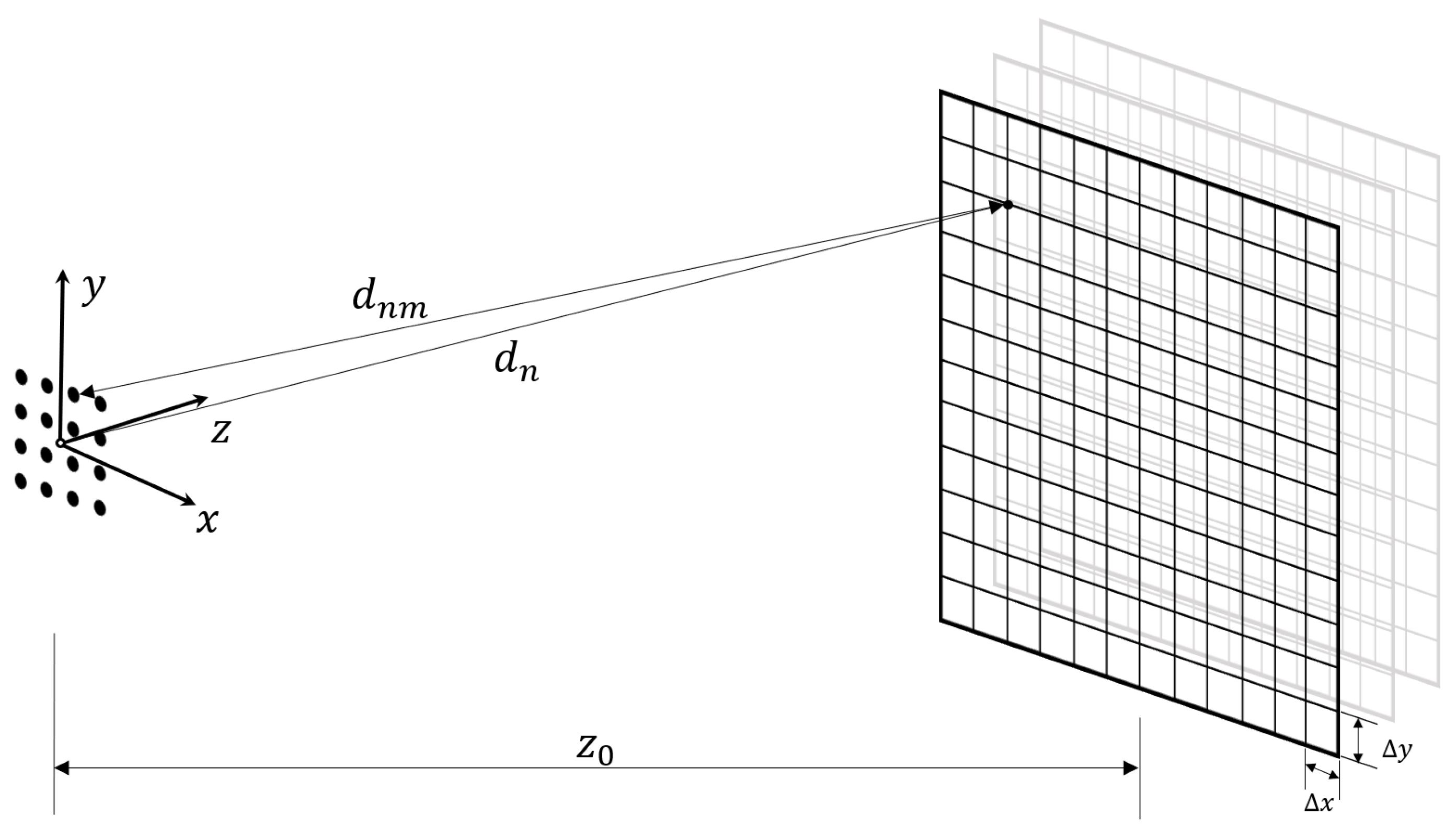
As shown in
Figure 1, a microphone array consists of
M microphones geometrically located at
. Suppose an unknown number of static point sources emitting wide-sense stationary sound signals in the three dimensional space. Suppose that an imaginary grid in the three-dimensional space has
N grid points locating at
,
.
Without a loss of generality, take the geometric center of the microphone array as the Cartesian coordinates’ origin, i.e., . Thus, the distance from each grid point to can be defined as , where denotes the Euclidean norm. The time difference of arrival (TDOA) between the received signals at and equals , where c denotes the speed of sound.
The microphone array’s steering vector to
can be written as
where
f and
denote the signal’s frequency and corresponding wavelength, respectively.
The array signal in the frequency domain can be expressed as
where
stand for the frequency spectral vector of
N uncorrelated sound signals at
;
,
denotes the
M-by-
N array manifold matrix; and
denotes the additive noise on the microphones that is uncorrelated with
, and has the spatially identical power spectral
.
With
in Equation (
2), the cross-spectral matrix (CSM) of the array signal equals
where
,
are the CSM’s of the source signals and the noise, respectively.
stands for the signal power at the
n-th grid point.
denotes the diagonal matrix, and
represents the
M-order identity matrix.
Since the theoretical
in Equation (
2) can be hardly obtained, it is generally estimated by a certain number of consecutive snapshots (a frame) in the time domain.
denotes the array signal spectrum estimated from the
k-th frame, for
. Thus, the CSM of the array signal can be estimated by
where
and
are unknown.
The output of the DAS beamformer steering towards the
n-th grid point equals
where
is known as the
point spread function, and
is the DAS beamformer weight vector constrained by
.
With
in Equation (
5), stacking the beamfomrer outputs towards all of
gives
where
and
. Note that
is a constant vector determined by the locations of all grid points
and the locations of all microphones
.
When the noise power
is sufficiently low, Equation (
7) implies that
Generally in acoustic imaging and sound source localization, the number of grid points is much larger than the number of sources, i.e.,
. The sounds sources are presumed sparsely distributed on the grid. Thus, the vector
in Equation (
7) is generally sparse. The general problem is to determine
from the DAS beamformer outputs
.
4. Numerical Simulations
In the numerical simulations, a circular microphone array of 1 m radius with microphones is used. A square grid ( grid points) spanning a 4 m × 4 m plane parallel to the circular array at a distance of 2 m is set. The proposed algorithm adopts a disk-shaped structuring element of the radius equal to 2 grid points. The simulations are conducted on a laptop with an AMD Ryzen 7 5800H 3.20 GHz processor.
For the
i-th iteration in Equation (
26), the per-grid-point standard deviation of source mapping error is defined as [
26]
Define the total sound power on all grid points before applying the proposed algorithm as
Define the total sound power on all grid points after applying the proposed algorithm as
Define the total sound power on the grid points within a circle
centered at a specific
as
With the above definitions in Equations (
28) and (
30), respectively, define the overall level error, the specific level error, and the inverse level error as [
23]
which evaluates the performance of the proposed algorithm to pinpoint all sources, to pinpoint the major sources, and to separate the major sources.
To evaluate the performance of the proposed algorithm, DAMAS, DAMAS-CG2, DAMAS-CG3 and DAMAS2-v are simulated for comparison. Note that DAMAS-CG2, DAMAS-CG3 and the proposed algorithm set for the non-selected grid points, which inherently improves performance in terms of , and .
Gauss–Seidel iterations in Equation (
26) and
in Equation (
27) are applied to ensure the algorithm convergence. Define an algorithm’s running time relative to that of DAMAS as
T. That is,
for DAMAS.
4.1. Scenario 1: Single Source
In this scenario, only a single sound source with
is presumed. In each of the 1000 Monte Carlo realizations, the sound source locates at the grid point
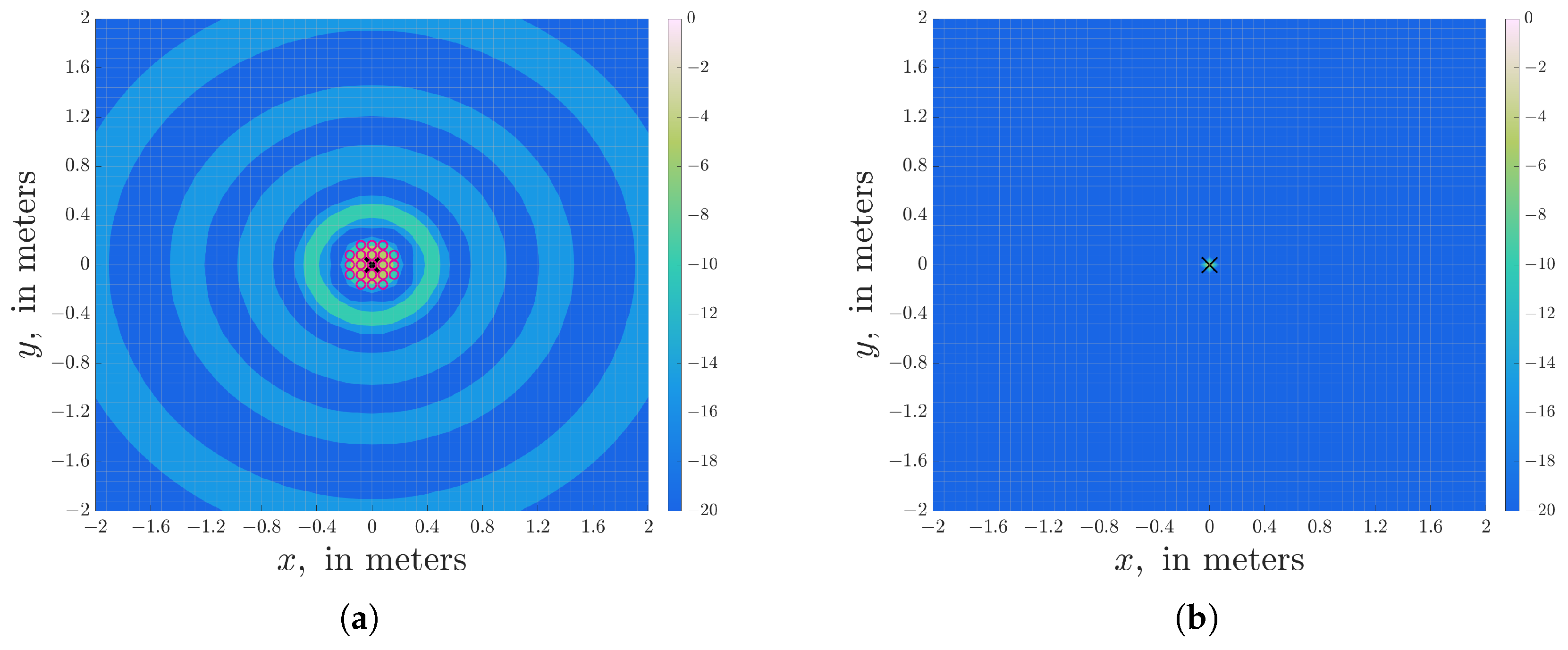
. The constructed acoustic images by the DAS beamforming in
Figure 2a, and the proposed algorithm in
Figure 2b are shown. The
selected grid points by the morphological reconstruction of a proposed algorithm are shown as blue circles in
Figure 2a.
The performance metrics are summarized in
Table 1. Taking the algorithm time of DAMAS as the reference (100%), DAMAS-CG2 has over 40% algorithm time, DAMAS-CG3 has 11.44% algorithm time, and DAMAS2-v has 15.55% algorithm time (and the proposed algorithm reduces this number to 8.06%). Apparently, the proposed algorithm generates the acoustic image with the localization accuracy comparable to the other algorithms, but with the algorithm time lower than the others.
4.2. Scenario 2: Triple Sources with Unequal Power
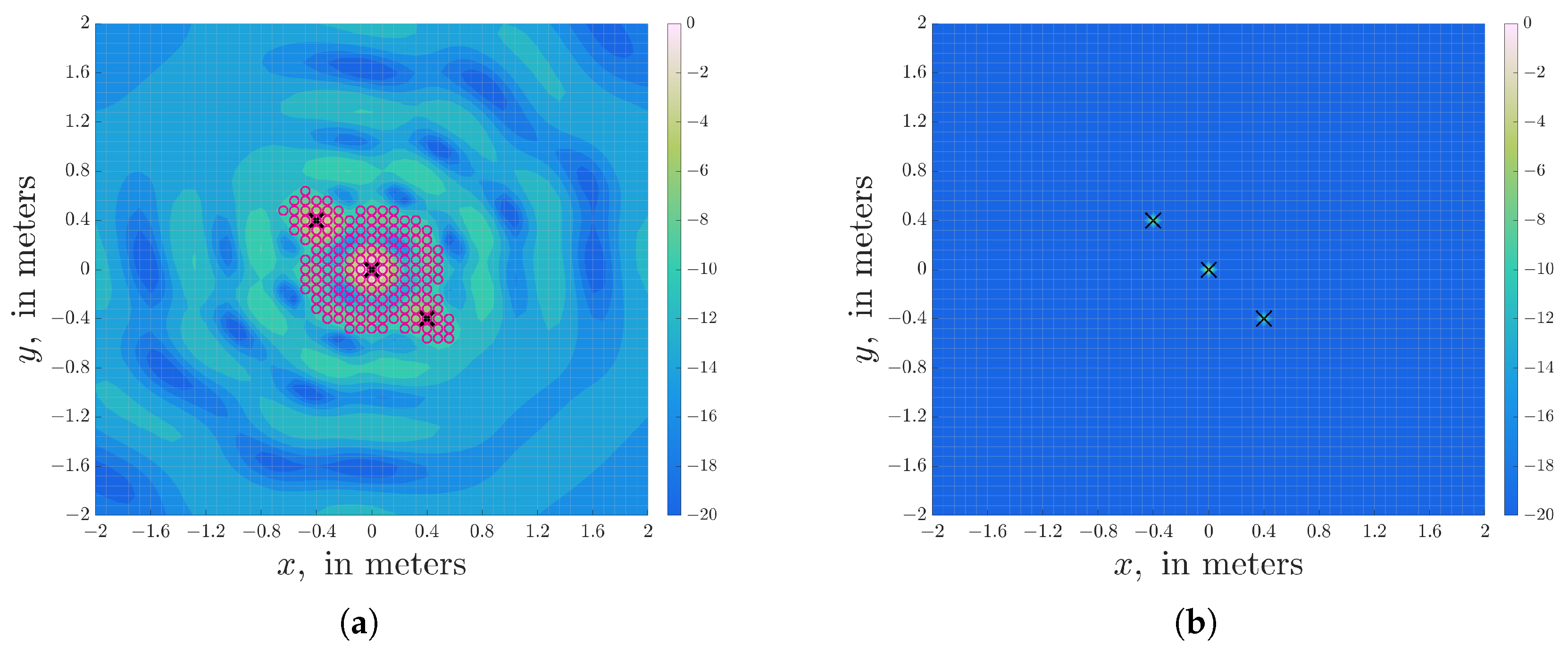
In this scenario, three sources are set. In each of the 1000 Monte Carlo realizations, the sound sources are fixed at the grid points , and with intensity level , and , respectively.
The algorithm performance is shown in
Figure 3 and
Table 2, similarly to that in
Section 4.1. This simulation confirms that the proposed algorithm outputs an accurate acoustic image by not neglecting the weaker sources.
4.3. Scenario 3: Many Sources
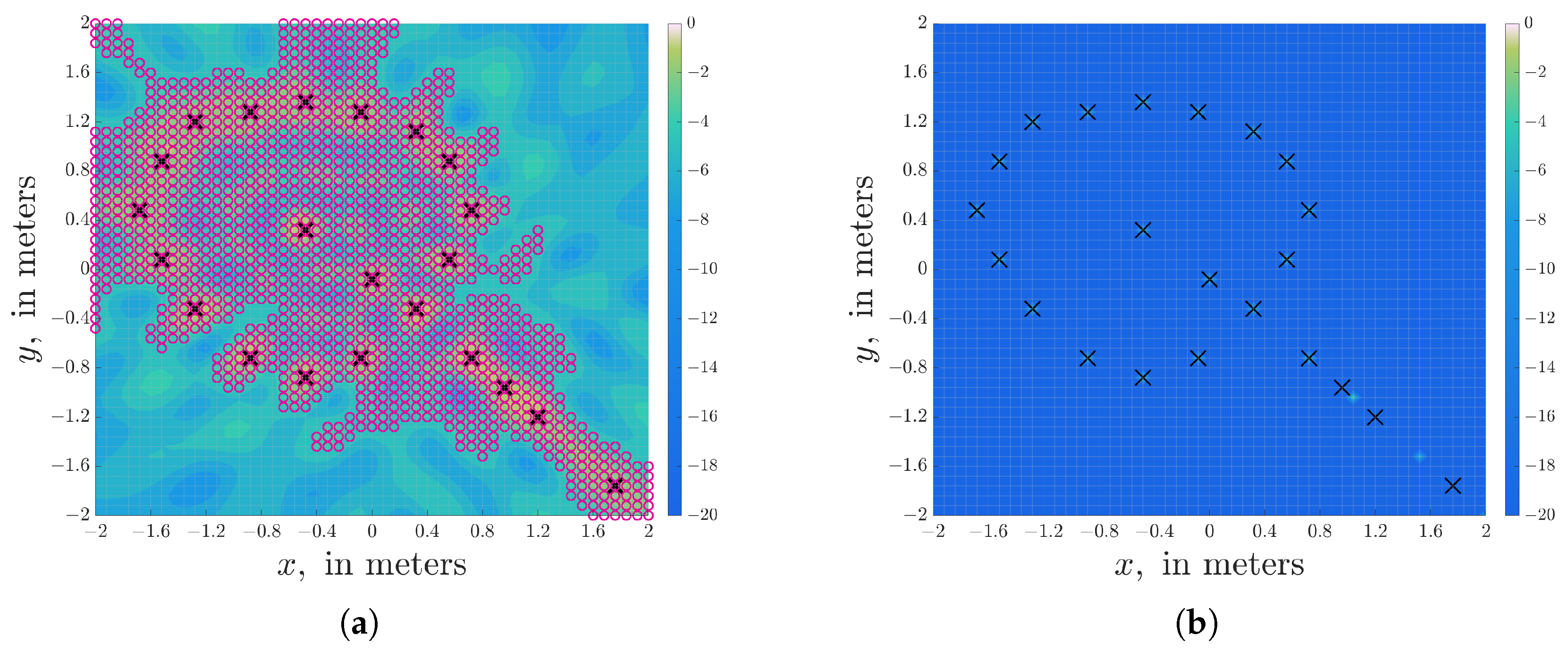
In this scenario, 22 spatially distributed sources with center frequency of 2 kHz and identical power
are employed, as indicated by the black ’x’ icons in
Figure 4. The algorithm performance is shown in
Figure 4 and
Table 3, similarly to that in
Section 4.1. In this very adverse scenario with many sources, the proposed algorithm has a comparable accuracy in acoustic imaging to DAMAS-CG3, but with only about 38% of computation load of DAMAS-CG3. Although DAMAS2-v reduces the algorithm time to 7.85%, which is lower than that of the proposed method, its localization performance drops substantially in this scenario.
4.4. Ablation Experiments
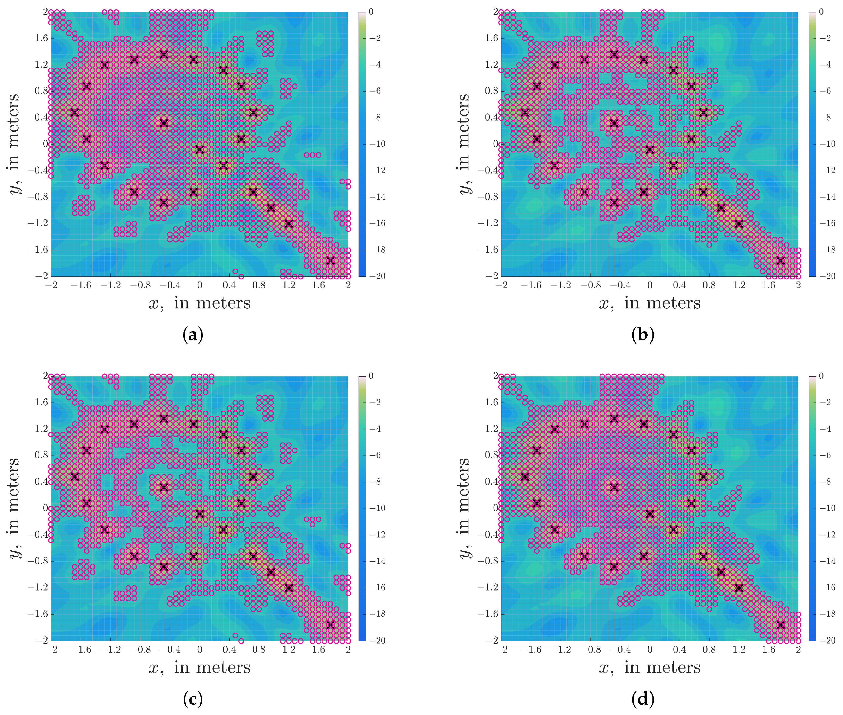
The proposed method comprises three modules: opening by reconstruction, closing by reconstruction, and Otsu’s method. In scenario 3, ablation experiments are performed in three configurations: without opening by reconstruction, without closing by reconstruction, and without both of the two reconstruction operations.
The performance of the algorithm under different configurations is shown in
Table 4. All schemes achieve comparable localization performance and exhibit only slight difference in computational time.
The method without opening by reconstruction has no obvious change in running time, yet it results in incomplete removal of non-sound-source regions, as displayed in
Figure 5a. The method without closing by reconstruction requires less running time than the proposed method, but it causes hollow cavities to emerge inside sound-source regions, as displayed in
Figure 5b. When both reconstruction morphological operations are discarded and only Otsu’s method is applied, the running time decreases. Nevertheless, this approach simultaneously induces hollow cavities inside sound-source areas and fails to fully eliminate non-sound-source regions, as displayed in
Figure 5c.
Consequently, the combination of all three steps guarantees that the extracted sound-source regions are the most complete and accurate, as displayed in
Figure 5d.
5. Empirical Experiments
Practical experiments are conducted in both the indoor and the outdoor scenarios. A
square microphone array is used for real-data acquisition, with a inter-microphone distance of 0.1 m.
Gauss–Seidel iterations in Equation (
26) and
in Equation (
27) are applied to ensure the algorithm convergence. Four NI-9234 data acquisition cards together with an NI-9184 CompactDAQ build the A/D conversion system with the 16-channel simultaneous sampling rate of 51.2 kHz.
In the real environment experiments, the sound source power can be hardly determined due to the background noise, the noticeable reverberation, and the nonideal measurements. Consequently, the metrics
,
,
, and
in
Section 4 cannot be obtained. Instead, the average source localization error
is used to assess the accuracy of acoustic imaging, where
represents the source position,
J denotes the source number, and
signifies the grid point position as the estimate of
. To assess the grid compression performance, the proposed algorithm is compared with DAMAS-CG2 and DAMAS-CG3 using the empirical data. DAMAS with no grid compression is taken as the reference.
5.1. Scenario 4: Indoor Experiment
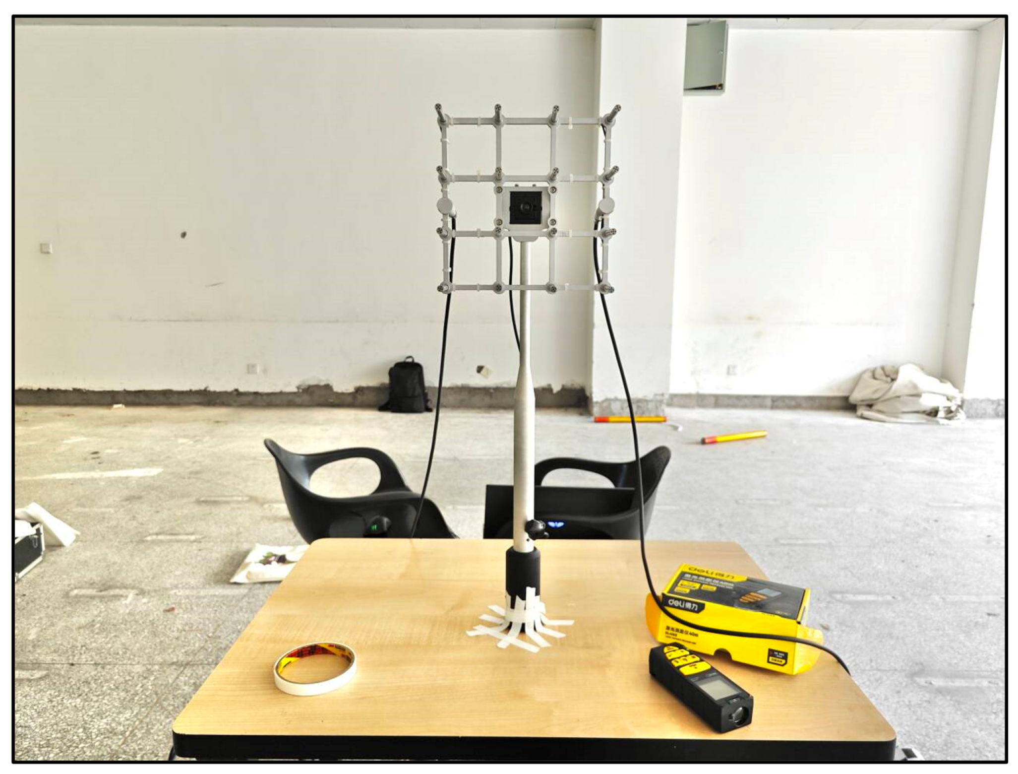
The indoor experiment is carried out in a shoebox-shape classroom at the Wangjiang Campus of Sichuan University, with
m in length,
m in width, and
m in height, as shown in
Figure 6. A handheld smartphone playing a 2 kHz pure tone signal simulates a single source. The microphone array faces the wall at 1 m distance. The primary background noise comes from the central air conditioning system and the bird calls outside the windows. The sound level meter shows the average environmental noise level is around 45 dB. The virtual grid of
points is on the wall plane spanning an area of
m in length and
m in width.
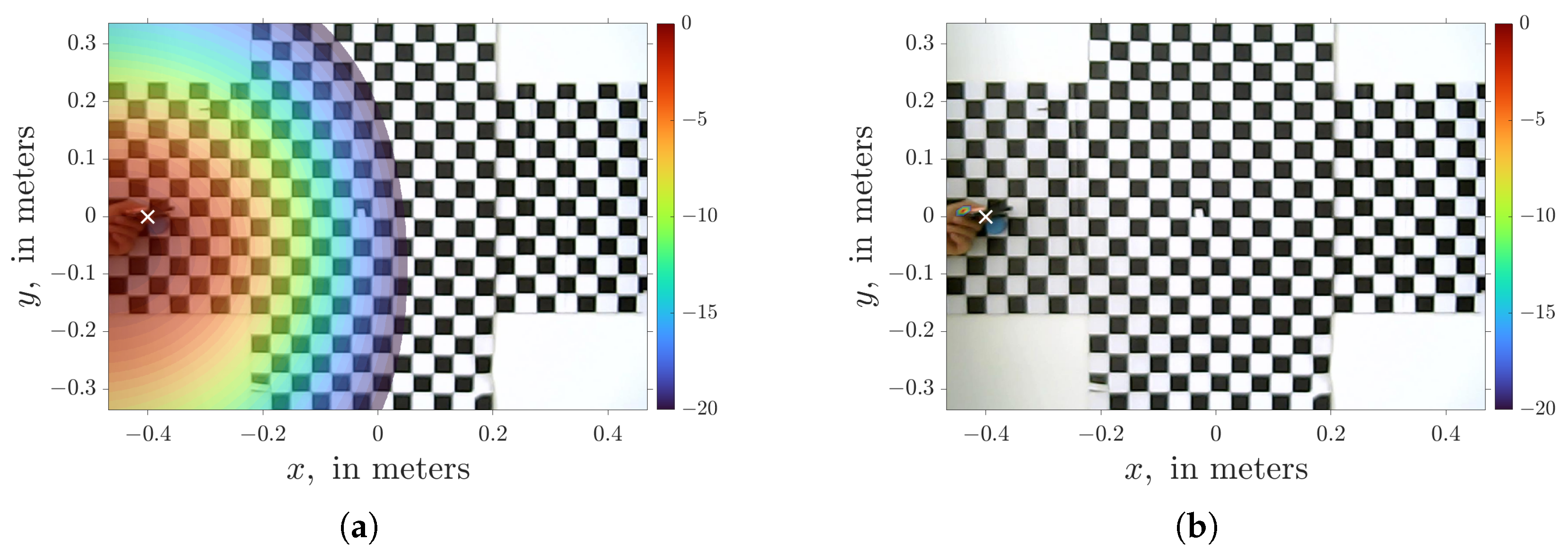
The acoustic image by the DAS beamformer and the proposed algorithm are shown in
Figure 7a,b. The source localization error and algorithm time of the competing algorithms are shown in
Table 5. It can be seen that the localization errors of various algorithms are at the same level, while the proposed algorithm has the lowest relative algorithm time of
, which is only about
of DAMAS-CG3, and
of DAMAS and DAMAS-CG2. Apparently, the significantly lower
is one major reason for this reduction.
5.2. Scenario 5: Outdoor Experiment
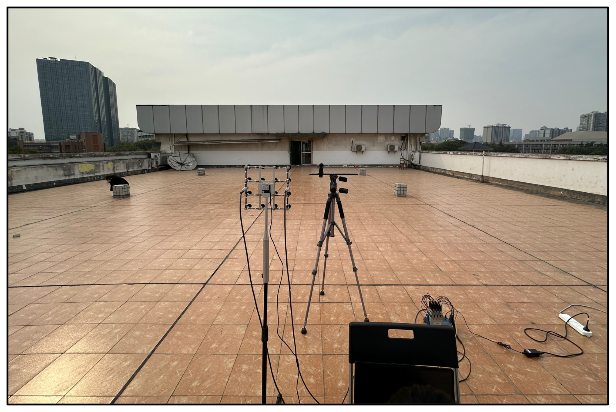
The outdoor experiment with the same microphone array in
Section 5.1 is conducted on the rooftop of a teaching building, as shown in
Figure 8. The outdoor environment has a 55 dB background noise, primarily due to the wind weather. A wireless loudspeaker controlled by a smartphone via the Bluetooth connection plays a 2 kHz pure tone signal. Meanwhile, another handheld smartphone playing the same pure tone signal acts as another sound source. The same grid as in
Section 5.1 is set on a rectangular plane of
m
2 at 1 m distance from the microphone array.
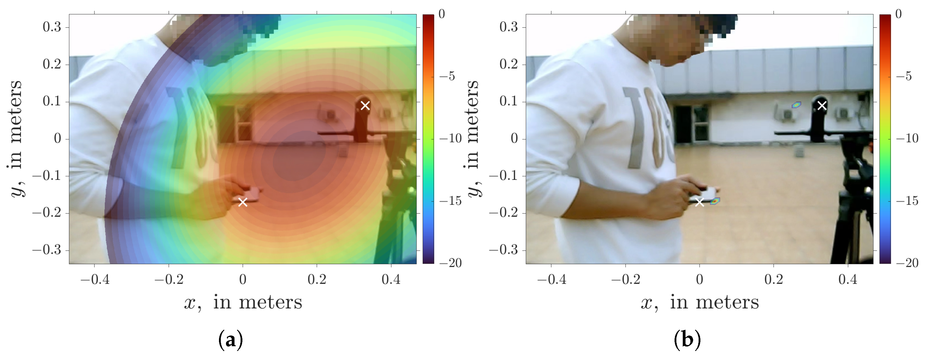
The acoustic image by the DAS beamformer and the proposed algorithm are shown in
Figure 9a,b. Apparently, the DAS beamformer cannot separate and locate the two sources in
Figure 9a due to the single broad peak of
. On the other hand, the proposed algorithm successfully separates the two sound sources with a high spatial resolution. The average localization error and relative algorithm time of the competing algorithms are summarized in
Table 6. Surprisingly, the proposed algorithm achieves the lowest localization error with only
to
algorithm time of the other deconvolution approaches.