1. Introduction
Gene regulatory networks (GRNs) are understood as a set of interacting regulators existing in any cell of any living organism and responsible for any important functions, including morphogenesis, adaptation to changing in the environment, etc. The study of GRNs is a laborious process, which consists of gathering the experimental data, processing them, and making conclusions. Based on this analysis the mathematical model can be inferred that is to be used for a mathematical analysis and making conclusions that can help to understand the processes in a real GRN. Many papers have been prepared that provide the application of mathematical tools for the study of GRNs. They can be found in the review articles, which are numerous, including [
1,
2,
3,
4]. The mechanism of constructing a mathematical model from biological data is focused on in [
3,
5].
A convenient mathematical apparatus based on ordinary differential equations was proposed by Wilson and Cowan in [
6]. This system was designed to describe various interactions between two populations of neurons. Later, its
n-dimensional version was used in multiple contexts, and for the description of gene networks of arbitrary size also. This system is (
1) in the next section. It consists of a linear part and a nonlinear bounded one, so that all solutions are extendable to infinity. Due to its structure, it has an invariant set in the phase space, and trajectories are trapped by this set. Therefore it can have attractors, which play an important role in the mathematical modeling of a network. The evolution of a modeled network depends on the location, number and general properties of attractors. These attractors play an important role in the interpretation of the behavior of the solutions of a system.
The role of the study of genetic regulatory networks (GRNs) in the study of biomedical problems cannot be underestimated. In several articles, the reaction of a subnetwork of a GRN to the development of some diseases was considered, notably works [
7,
8,
9,
10], and others.
In [
11], the genetic regulatory network ruling the expression of the genes involved in the angioedema disease is illustrated by the scheme of connections. Additional analysis reveals that there are several attractors in the form of 11 fixed points and no periodic attractors. The pathologic attractor corresponding to the hereditary form of the disease has a relative size equal to about 5 of the possible states of the network. A particular attractor in the form of a fixed point has a basin of attraction that comprises 93.43 percent of the possible states of the network.
In [
9], the authors constructed an aging gene regulatory network consisting of the core cell cycle regulatory genes (including p53). They obtained a conceptual model for capturing three distinct stable steady states (or attractors) corresponding to homeostasis, cell cycle arrest, and senescence or apoptosis. In addition, they applied a computational method to quantify the potential landscape, which displays: (I) one homeostasis attractor for low accumulation of DNA damage; (II) two attractors for cell cycle arrest and senescence (or apoptosis) in response to high accumulation of DNA damage. The process of aging can be characterized by state transitions from landscape I to II. By in silico perturbations, the potential landscape of a perturbed network (inactivation of p53) was identified, and thereby the emergence of a cancer attractor was demonstrated. “The simulated dynamics of the perturbed network display a landscape with four basins of attraction: homeostasis, cell cycle arrest, senescence (or apoptosis) and cancer. Our analysis also showed that for the same perturbed network with low DNA damage the landscape displays only the homeostasis attractor”. The authors expressed the hope that “the mechanistic model offers theoretical insights that can facilitate discovery of potential strategies for network medicine of aging-related diseases such as cancer”.
In [
7,
8], the three-dimensional Wilson–Cowan type system was considered. The authors were interested in dynamical networks with coexisting attractors. They assumed that the system was static—that is, that it did not change the relations between the elements of a network—the basins of attraction were unchangeable. Given an initial condition, the system approached one of the attractors. This attractor had specific biological–medical significance, and it could be considered as “normal” (“physiological”) versus “undesired” (“pathological”).
The role of inhibitory and activatory cycles was emphasized. The general scheme of considering this topic was as follows. The current state of the networks was described by a trajectory emanating from a prescribed location. Future states were to a great extent associated with the location and number of attractors. One of the main questions to be answered was about the robustness of attractors concerning small perturbations. Another question was about how attractors change given gradual changes in the parameters. A realistic biological network was considered, “T-cells in large granular lymphocyte leukemia associated with the blood cancer”. A T-cell signaling survival network has 60 nodes and many edges. The nodes in the network represent proteins and transcripts, and the edges correspond to either activation or inhibitory regulations. The researchers found three attractors in the physiological network and three corresponding attractors in their model. Two of the physiological attractors were cancerous, and one was normal. In the model, they found multiple ways to drive the system to the normal state by changing the values of properly selected parameters.
In this note, we wish to consider a similar situation, considering a three dimensional Wilson–Cowan-type system that may have several coexisting attractors. We show how to drive the system from any selected attractor to any other. Thus, we demonstrate that in complex networks with multiple attractors and many elements this might be a usual process.
In the next section, we provide the necessary mathematical apparatus. Then we consider several examples and construct means for managing a system in a desired direction. Our conclusions and discussion follow. The examples are appropriately illustrated, and projections of attractors are visible.
2. System
The system we are studying is (
1):
where
are unknowns,
and
are parameters, and
are the entries of the so-called regulatory matrix
which is used to describe the interrelations between elements (nodes) of a network. The functions
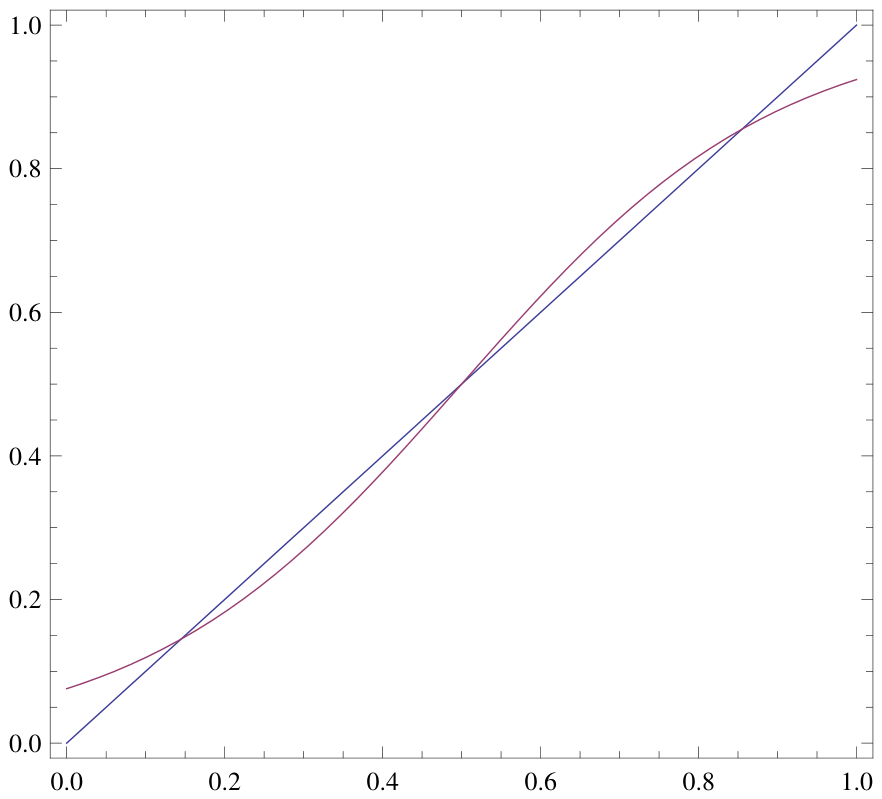
may be any sigmoidal functions: that is, monotonically increasing from zero to unity with exactly one inflection point. One such function is
There are
parameters in this system, which define the main properties.
Often system (
1) is used in the following form:
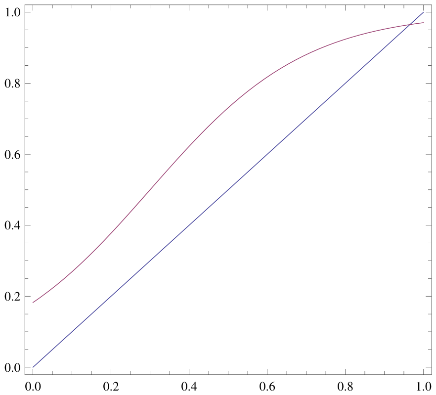
The parameters say how rapidly functions go to unity. Values create nonlinearities strong enough for diverse behaviors, such as switching, bistability, and oscillations. The parameters dictate locations of the graphs of with respect to horizontal direction. The coefficients define the natural exponential degradation rates of solutions, if f are identically zeros. The parameters shift the sigmoid horizontally. Changing moves the switching hyperplane, which affects: the number of equilibria, their stability, the locations of attractors, and transitions between regimes. Thresholds are crucial for control over the network.
Biologically, control how sharply gene i responds to its regulators; is the strength and sign of regulation of gene i by gene j (for instance, means activation, means repression); is the degradation rate of gene product i; is the activation threshold for gene i. Biologically, thresholds encode sensitivity.
System (
1) is quasi-linear, therefore all solutions are extendable to infinity. It possesses an invariant set
, which traps solutions. Mathematically this is the main reason for the existence of attractors in
The main properties of the system are dependent on the matrix
Various relations between
are dependent on the structure of
This matrix in realistic examples is sparse, so most of its elements are zero.
3. Materials and Methods
For the analysis of dynamical systems and the description of phase space, a geometric approach was used, based on the construction and analysis of nullclines. Attractors were identified and constructed during numerical experiments carried out using the Wolfram Mathematica program. The tools of the same program were used to create the images. The data for repeating the calculations and visualizing the results are provided in the text and in the figure captions.
Suppose that
are sigmoidal functions that monotonically increase from 0 to 1. Assume that generally nonlinear functions
are for the description of the relations between elements of a network. These elements have the characteristic
, which is dependent on the argument
t, interpreted as time. Solutions of system (
1) are meant as smooth functions
, satisfying the equations in (
1). The specific structure of system (
1) can be explained in the following way. It is assumed that elements of a network interrelate generally in a nonlinear way and that the
-th element is affected by the total effect of the remaining elements. To be realistic, this total effect is bounded. The second linear term
means the degradation of the
i-th gene expression product;
—the connection weight or strength of control of gene
j on gene
i. Positive values of
signify activating influences, whereas negative values denote repressing influences;
—the impact of external stimuli on gene
i is reflected in its ability to modulate the gene’s responsiveness to activating or repressing factors.
Definition 1. An invariant region in the phase space is the region that cannot be left by a trajectory of the system (1). Proposition 1. The set is an invariant set.
Consider the system of equations
Proposition 2. System (4) has a solution in the invariant set Sketch of the Proof. On the border of the invariant set vector field is directed inward. Therefore, the continuous map maps the topological ball onto itself. So the map has a fixed point in □
Definition 2. A set of points defined by the relation is called an i-th nullcline of the system (1). Definition 3. The cross points of all nullclines are called the critical points of system (1). Corollary of Proposition 2. System (1) has a critical point in an invariant set . Proposition 3. All critical points of system (1) are in the invariant set Proof. Any critical point belongs to all nullclines. Any nullcline lies in the strip for some These strips intersect by the set □
Remark 1. System (1) has at least one critical point but can have multiple critical points. Critical points are subject to analysis. The standard analysis of a critical point involves the following procedure.
Standard analysis. The goal is to obtain a vector that consists of characteristic numbers. The characteristic numbers, with some degenerate cases, provide information on the type of a critical point.
This can be done effectively for system (
3). Consider this system (for brevity) in a three-dimensional setting (
are set to 1)
Critical points are solutions of the system
Linearization at a critical point
gives
where
It follows from (
6) that
Then
for
and the coefficient matrix
A of the linear system (
7) can be written in the form
The characteristic equation
where
E is the unity matrix, is then a cubic equation with coefficients expressed explicitly in terms of the critical point.
4. Results
The phase space of the system (
1) contains possible states of a network. The current state of a network is described by the vector
, which depends on time. The attractors of the system are geometrical formations of various shapes, which can be revealed by tracing trajectories with the appropriate initial conditions. The phase space is decomposed to several basins of attraction of these trajectories. The problem of reconfiguring the phase space (in fact, only the invariant set
) is the most important. Given the current state
at the moment
, one might face the problem of sending the trajectory to a selected region of
(to an attractor, which is normal in the context of the studied problem). The three examples in the Introduction are of this kind. Geometrically, this problem is one of intercepting the current trajectory, which goes to a “wrong” attractor, and redirecting it to a “normal” attractor. For this, any adjustable (in the context of a problem) parameters can be used.
4.1. Intercepting Trajectories: The Case of Fixed Point Attractors
Let a network be modeled by a system
The nullclines are obtained from the relations
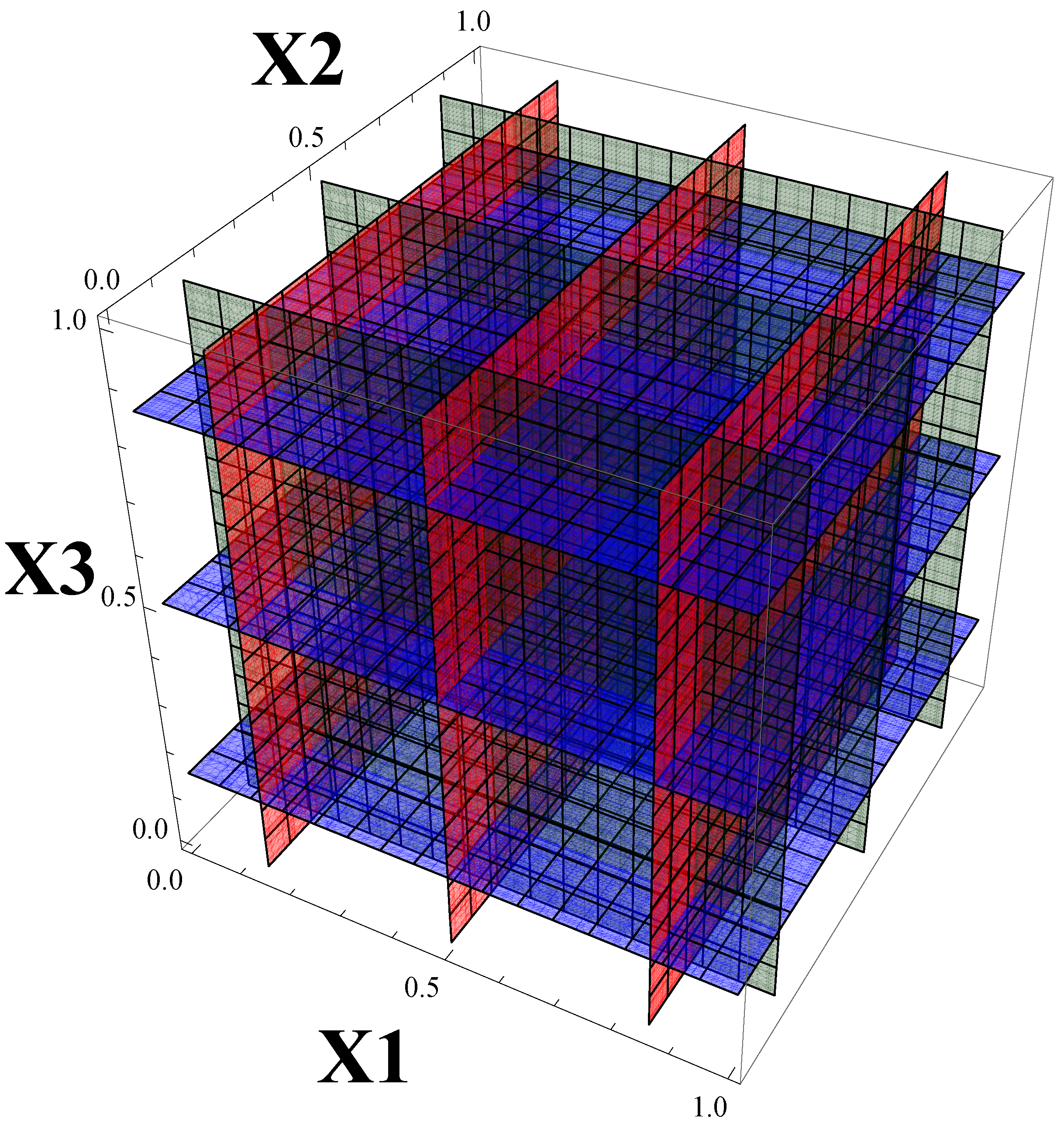
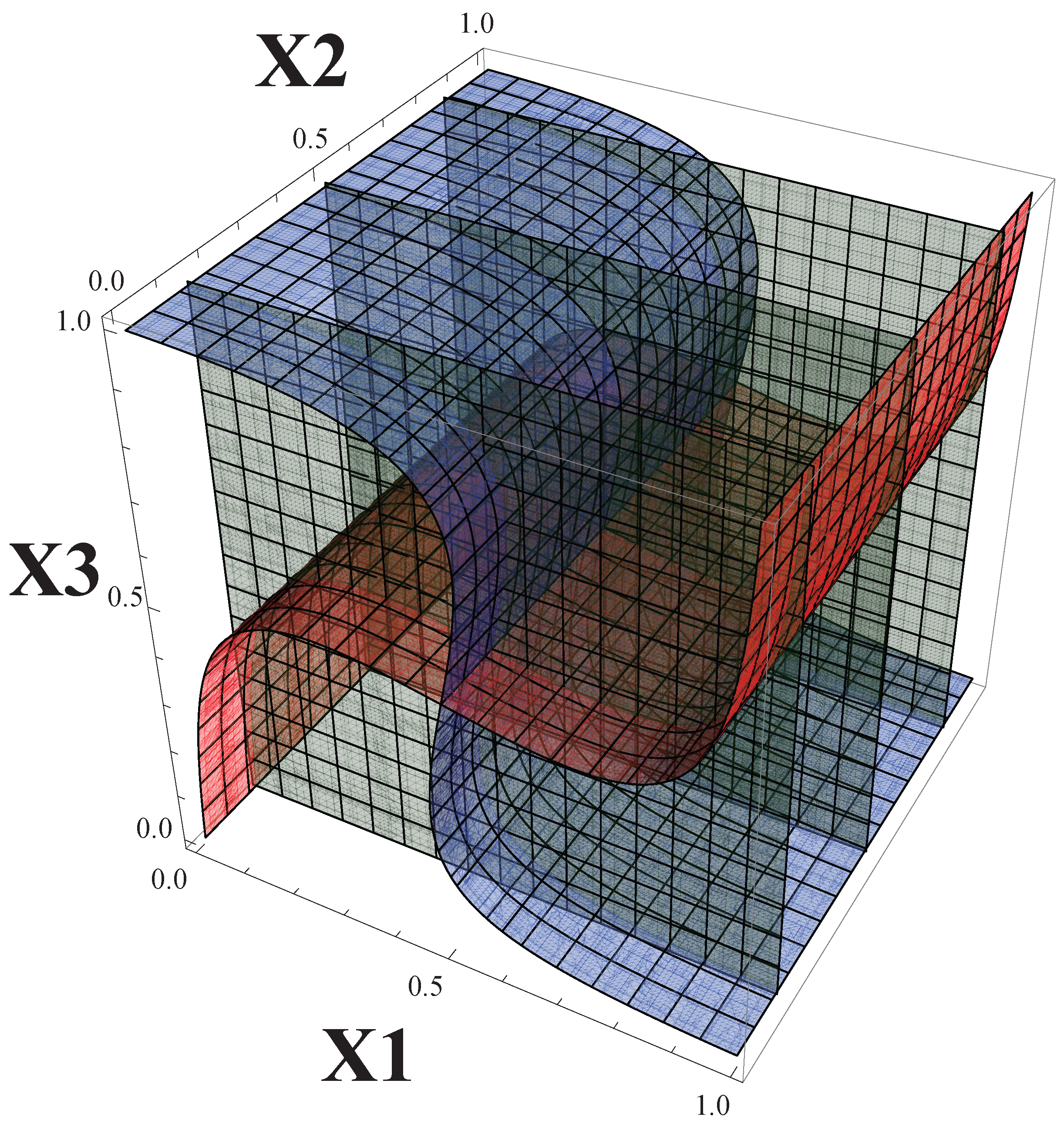
Geometrically these nullclines are three mutually orthogonal sets by three parallel planes, as is ilustrated by
Figure 1 together with
Figure 2.
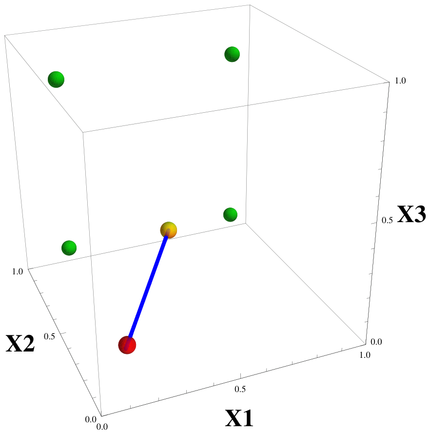
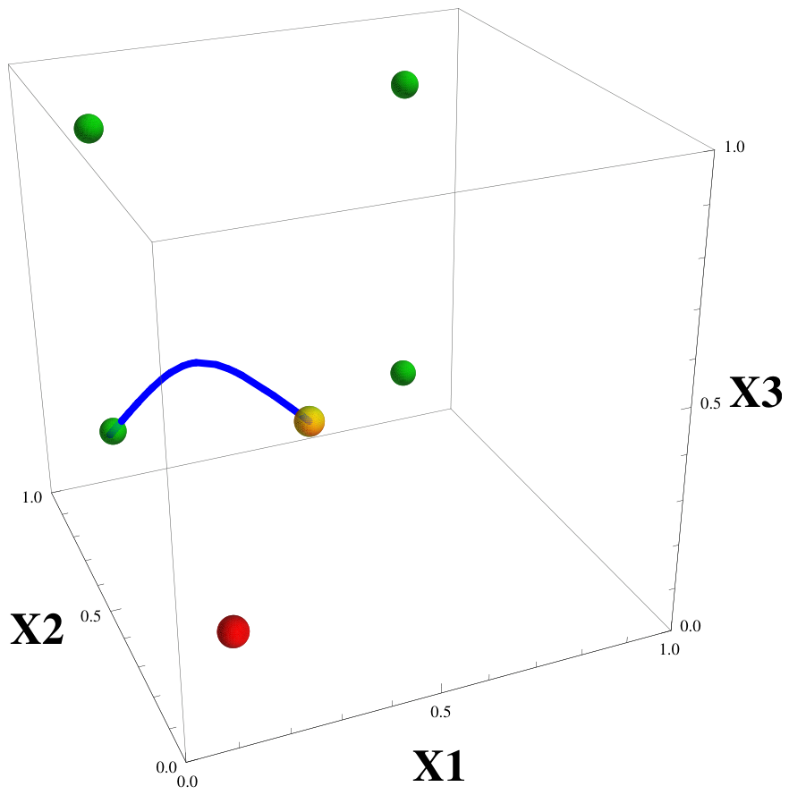
There are several conditionally “normal” attractors (green) and one “pathogenic” (red). The current state of a network is marked in
Figure 3 by the yellow point at
The trajectory goes to the red point (“pathogenic”). The problem is to re-send the trajectory from its current location to one of the normal attractors. How to solve it? If the geometry of nullclines is known, this is possible. Notice that all the marked points are at the intersection of all the nullclines. If one of the components of the
-nullcline is eliminated, the “pathogenic” attractor will be eliminated too.
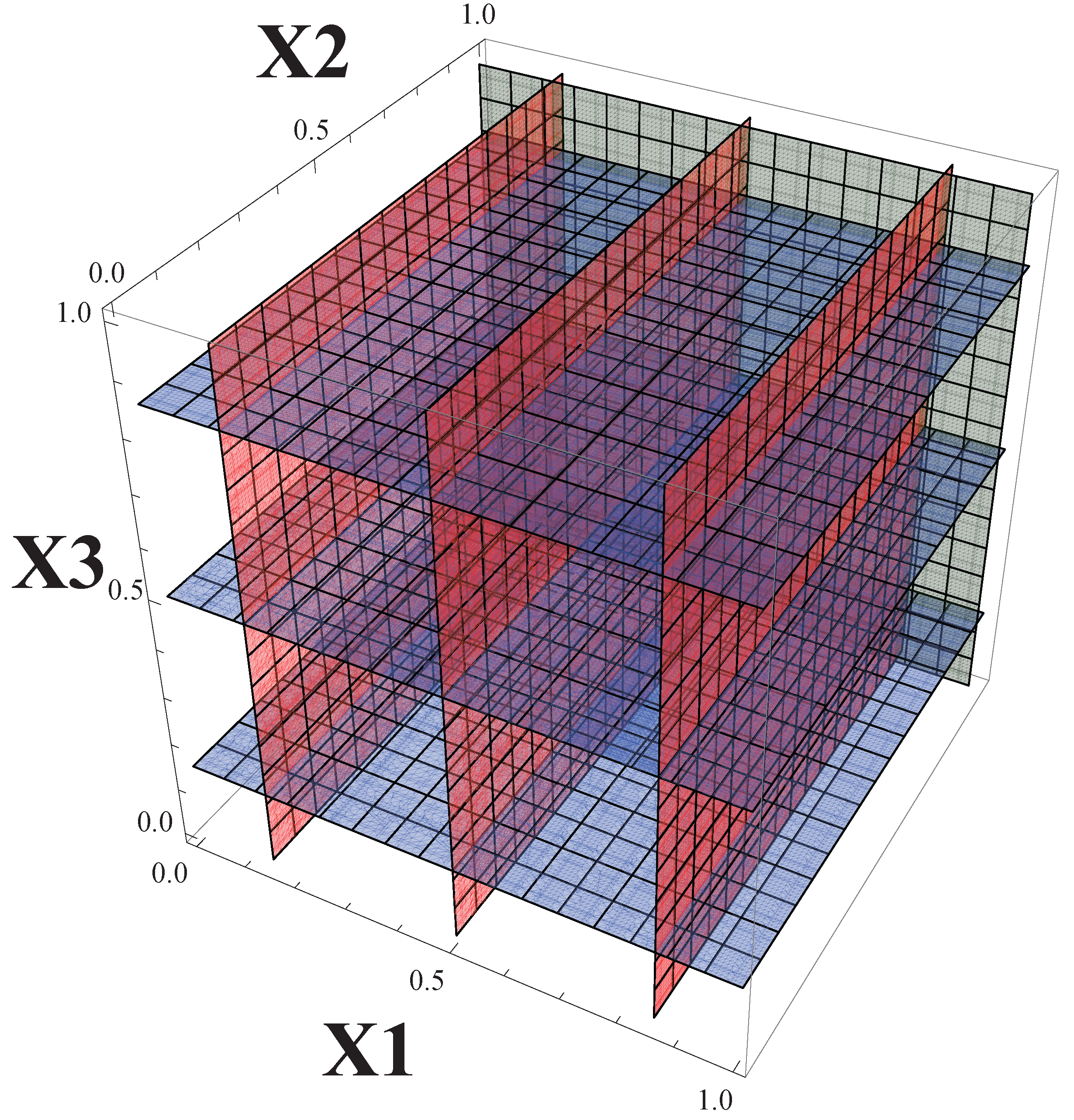
By changing the parameter
to the value 0.3 the
-nullcline is reduced to only one plane that is defined by
The “normal” attractors (green) are slightly shifted, but all four exist. The trajectory in the absence of the “pathogenic” attractor tends to the nearest “normal” one. This process is illustrated by
Figure 1,
Figure 2,
Figure 3,
Figure 4,
Figure 5 and
Figure 6.
Remark 2. In the preceding example, the locations of the “normal” attractors are changed compared with the initial configuration. This can be corrected. Once it is detected that the trajectory is close enough to a “normal” attractor, all parameters that were changed are to be restored. The trajectory is now in a basin of attraction of a “normal” attractor and the problem is resolved. This attractor is at (0.145, 0.885, 0.145). It is a stable node also with a triple λ = −0.380856.
4.2. Intercepting Trajectories: Periodic Attractors
Consider the system
The nullclines are defined as
The second nullcline is a set of three planes parallel to the
-plane. The nullclines are depicted in
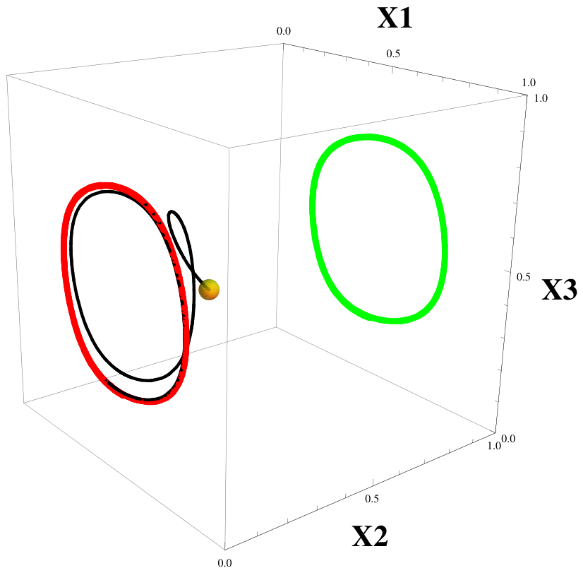
Figure 7. The attractors are two closed trajectories that are seen in
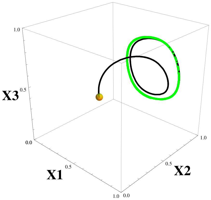
Figure 8 together with the trajectory emanating from the point
This trajectory is attracted by an attractor depicted in red. It is assumed to be “pathogenic”. The problem is to redirect this trajectory to a green attractor, which is also a closed trajectory. It is considered as “normal”.
The parameter
is changed to the value
The result is seen in
Figure 9.