An Age-Structured Model for COVID-19 Hospitalization Rate

Abstract

In this study, an age-structured framework is developed to model post-pandemic COVID-19 hospitalization rates. A partial differential equation (PDE) incorporating age-specific information is first formulated and analyzed. Based on this PDE, a physics-informed neural network (PINN) is constructed and calibrated using real-world data. Through this integration, mathematical rigor is combined with the adaptability of machine learning (ML), resulting in an interpretable approach that leverages physical principles while reducing the opacity typically associated with ML-based models.

1. Introduction

COVID-19 has been a prominent issue for the past five years, disrupting society and having a significant economic impact [1]. Since the pandemic, all countries have invested significant resources to monitor the spread of the virus, and different monitoring systems have been developed, see for example [2,3,4]. These systems provide valuable data for experts to understand the progression of the pandemic and help the government make public health policies.

One way to assist stakeholders is to provide an accurate prediction of the pandemic trend. Therefore, predictive models are in high demand, and many scholars have investigated this problem and made significant progress in the field. For example, a popular modeling methodology for COVID-19 is the compartmental model, which divides the population into multiple compartments, such as Susceptible (S), Infected (I), and Recovered (R), and models the rate of change of each compartment using ordinary differential equations (ODEs). The reader is referred to [5,6,7,8,9,10,11,12,13,14,15,16,17] and the references therein for recent advancements in this area, as well as for compartment epidemic models in general.

In May 2022, the World Health Organization (WHO) declared an end to COVID-19 as a public health emergency [18]. Humanity has gradually resumed normal life and adapted to coexisting with the virus. However, developing new models to understand post-pandemic transmission trends remains crucial. As shown in Figure 1, hospitalization rates vary significantly across different age groups. To capture age-specific differences within the compartments, age-structured models have been developed by many researchers. These models either use ODEs to model the compartments of different age groups, see for example [5,11], or use partial differential equations (PDEs) to model the age-density distribution of individuals within a compartment, see for example [15,17]. These compartment models have made significant contributions to understanding how the disease evolves. However, a major limitation remains: some compartments cannot be directly observed—for example, the Recovered (R) compartment. Some studies simply assume an initial value of zero, but the validity of this assumption remains debatable.

Motivated by this concern, we plan to incorporate age-specific information into our models and ensure that model components are observable, allowing better alignment with real-world data. It is well known that model calibration is essentially an inverse problem and typically requires significant computational resources. To address this challenge, we will adopt optimization techniques developed in the field of machine learning (ML).

Mathematical models are typically derived through rigorous analysis, where each component has a well-defined role. However, traditional models often assume that all components are either constants or functions with “nice” properties (e.g., differentiable). These simplifications facilitate qualitative analysis but may not fully capture real-world complexity. The adoption of ML allows us to approximate complicated functions that reflect this complexity. Despite their superior performance, ML models also have limitations. For example, most neural networks (NNs) have highly complex architectures, making it difficult to interpret their mechanisms; they are often regarded as “black boxes”. Reducing model opacity is therefore another goal of our work.

In this paper, we aim to leverage the strengths of both ML and mathematical modeling to address these limitations. Specifically, we will first develop an age-structured PDE model, following a rigorous mathematical modeling procedure, to describe post-pandemic COVID-19 hospitalization rates. Then, we will design an ML model based on the PDE framework and train it using real-world data. These models, known as physics-informed neural networks (PINNs), integrate physical laws into neural networks, enhancing both interpretability and predictive accuracy. The reader is referred to [19,20,21] for more details on PINNs. It is noteworthy that we will concentrate on hospitalization rates rather than case counts, as many people now choose not to report COVID cases. Consequently, surveillance reports on case numbers are less accurate than hospitalization data.

The remainder of the paper is organized as follows: in Section 2, we develop the age-structured PDE model and conduct a mathematical analysis on the model. The PINN model is developed in Section 3. A simulation is also given in that section. Finally, Section 4 contains the conclusions and discussions.

2. Age-Structured PDE Model for COVID-19 Hospitalization Rate

In this section, we develop the mathematical model. Throughout this paper, we denote the total population in a region by N, the maximum possible age by $a^{+}$, the age-specific death rate by $\mu \left(a\right)$, and the density function of the age distribution by $A\left(a\right)$, where $a\in [0,a^{+}]$. All these data can be readily obtained from online public datasets.

Let $H:[0,\infty )\times [0,a^{+}]\to \mathbb{R}$ be the COVID-19 hospitalization rate. To address the aforementioned challenge on data availability, we only consider two compartments: the hospitalized population due to COVID-19 and others. With our assumptions, a cohort of hospitalized patients of ages in the interval $[a,a+\Delta a]$ at time t due to COVID-19 can be expressed by

$$\begin{array}{c}\hfill h(t,a,\Delta a)={\int }_a^{a+\Delta a}NA\left(\tau \right)H(t,\tau )d\tau .\end{array}$$

(1)

Then the cohort of other individuals of ages in the interval $[a,a+\Delta a]$ at time t is denoted by

$$\begin{array}{c}\hfill u(t,a,\Delta a)={\int }_a^{a+\Delta a}NA\left(\tau \right)(1-H(t,\tau ))d\tau .\end{array}$$

(2)

Clearly, the cohort of the individuals of ages in the interval $[a,a+\Delta a]$ at time t, denoted by $n(t,a,\Delta a)$ satisfies

$$\begin{array}{c}\hfill n(t,a,\Delta a)={\int }_a^{a+\Delta a}NA\left(\tau \right)d\tau =u(t,a,\Delta a)+h(t,a,\Delta a).\end{array}$$

We assume that the COVID-19-related hospitalized patients are discharged by a rate that is proportional to the hospitalized patients $h(t,a,\Delta a)$, with an age-specific removal coefficient $\gamma \left(a\right)$, in addition to the natural death rate $\mu \left(a\right)$. We further assume that the COVID-19-related patients are hospitalized at a rate that is proportional to the unhospitalized population with an age-specific coefficient $\alpha \left(a\right)$. Then the change of the cohort $h(t,a,\Delta a)$ satisfies

$$\begin{array}{c}\hfill {\displaystyle \frac{h(t+\Delta t,a+\Delta t,\Delta a)-h(t,a,\Delta a)}{\Delta t}}=\alpha \left(a\right)u(t,a,\Delta a)-(\mu \left(a\right)+\gamma \left(a\right))h(t,a,\Delta a).\end{array}$$

When $\Delta t\to 0$, we have

$$\begin{array}{c}\hfill {\displaystyle \frac{\partial h(t,a,\Delta a)}{\partial t}}+{\displaystyle \frac{\partial h(t,a,\Delta a)}{\partial a}}=\alpha \left(a\right)u(t,a,\Delta a)-(\mu \left(a\right)+\gamma \left(a\right))h(t,a,\Delta a).\end{array}$$

Then by (1) and (2),

$$\begin{array}{c}\hfill {\int }_a^{a+\Delta a}NA\left(\tau \right){\displaystyle \frac{\partial H(t,\tau )}{\partial t}}d\tau +{\int }_a^{a+\Delta a}N{\displaystyle \frac{\partial \left[A\right(\tau \left)H\right(t,\tau \left)\right]}{\partial \tau }}d\tau \\ \hfill =\alpha \left(a\right){\int }_a^{a+\Delta a}NA\left(\tau \right)(1-H(t,\tau ))d\tau -(\mu \left(a\right)+\gamma \left(a\right)){\int }_a^{a+\Delta a}NA\left(\tau \right)H(t,\tau )d\tau .\end{array}$$

Multiply both sides by ${\displaystyle \frac{1}{\Delta a}}$ then let $\Delta a\to 0$, by the fundamental theorem of calculus, we have

$$\begin{array}{cc}\hfill NA\left(a\right){\displaystyle \frac{\partial H(t,a)}{\partial t}}+& N{\displaystyle \frac{\partial \left[A\right(a\left)H\right(t,a\left)\right]}{\partial a}}\hfill \\ \hfill & =\alpha \left(a\right)NA\left(a\right)(1-H(t,a\left)\right)-\left(\mu \right(a)+\gamma (a\left)\right)NA\left(a\right)H(t,a).\hfill \end{array}$$

To simplify the notation, when the context is clear, we will denote

$$H=H(t,a),{\displaystyle \frac{\partial H}{\partial t}}={\displaystyle \frac{\partial H(t,a)}{\partial t}},{\displaystyle \frac{\partial H}{\partial a}}={\displaystyle \frac{\partial H(t,a)}{\partial a}},\mathrm{and}{H}^{\prime }={\displaystyle \frac{dH\left(a\right)}{da}}.$$

We further assume $A\in C^1[0,a^{+}]$ and $A\left(a\right)>0$ on $[0,a^{+}]$. Then

$$\begin{array}{c}\hfill {\displaystyle \frac{\partial H}{\partial t}}+{\displaystyle \frac{\partial H}{\partial a}}+{\displaystyle \frac{A^{\prime }\left(a\right)}{A\left(a\right)}}H=\alpha \left(a\right)(1-H)-(\mu \left(a\right)+\gamma \left(a\right))H.\end{array}$$

(3)

Finally, we generalize $\alpha \left(a\right)$ in (3) by $\alpha (t,a)$ defined by

$$\begin{array}{c}\hfill \alpha (t,a)={\int }_0^{a^{+}}\beta (a,\nu )H(t,\nu )d\nu \end{array}$$

(4)

so that $\alpha$ can capture the impacts of COVID-19 patients across all age groups. This leads to the following age-structured model

$$\begin{array}{cc}\hfill & {\displaystyle \frac{\partial H}{\partial t}}+{\displaystyle \frac{\partial H}{\partial a}}=(1-H){\int }_0^{a^{+}}\beta (a,\nu )H(t,\nu )d\nu -\eta \left(a\right)H,0<a<a^{+},t>0,\hfill \end{array}$$

(5)

$$\begin{array}{cc}\hfill & H(0,a)=H_0\left(a\right),0\le a\le a^{+},\mathrm{and}H(t,0)=0,t\ge 0,\hfill \end{array}$$

(6)

where

$$\begin{array}{c}\hfill \eta \left(a\right)=\mu \left(a\right)+\gamma \left(a\right)+{\displaystyle \frac{A^{\prime }\left(a\right)}{A\left(a\right)}},\end{array}$$

and $H_0$ is the COVID-19 hospitalization rate at $t=0$ with $H_0\left(0\right)=0$.

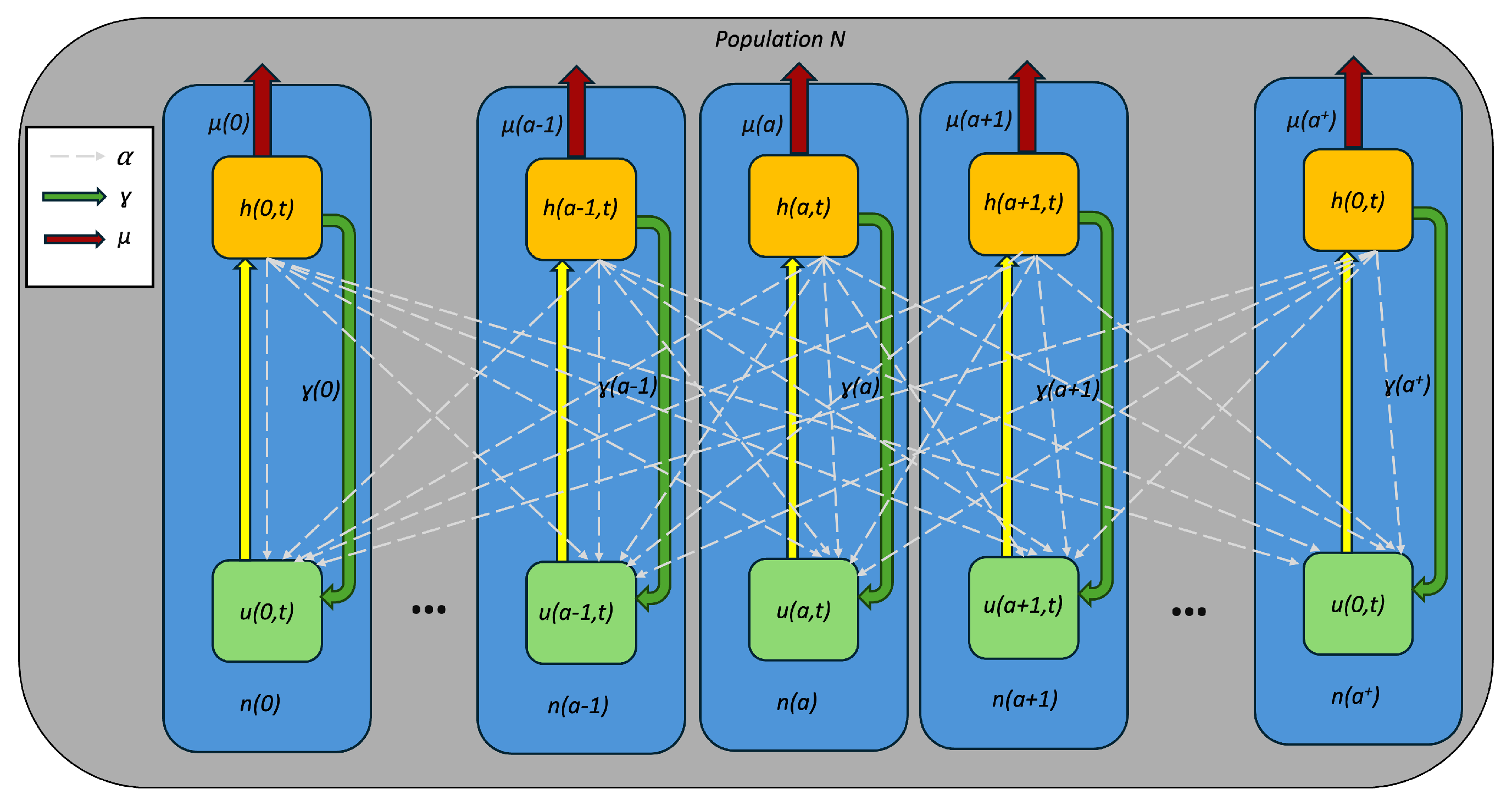
The relationship among all the cohorts is described by Figure 2. A summary of the notations used in the model is given in

Table 1. List of notations.

Notations	Meaning
N	Total population (constant)
$h(t,a,\Delta a)$	Cohort of hospitalized patients of ages in the interval $[a,a+\Delta a]$ at time t due to COVID-19
$u(t,a,\Delta a)$	Cohort of other individuals of ages in the interval $[a,a+\Delta a]$ at time t
$H(t,a)$	Hospitalization rate of age a at time t due to COVID-19
$A\left(a\right)$	Density function of the age distribution of N
$\mu \left(a\right)$	Per capita census death rate of age a of N
$\alpha \left(a\right)$	Entering coefficient of hospitalized patients of age a due to COVID-19
$\beta (a,\nu )$	Kernel to represent the impact to the patient cohort of age a from patient cohorts of age $\nu$
$\gamma \left(a\right)$	Removal coefficient of hospitalized patients of age a due to COVID-19

. All the notations are assumed to be nonnegative throughout this paper.

Remark 1.

The $\beta (a,\nu )$ in (4) is designed to capture the impacts of COVID-19 patients across all age groups. The hospitalization rate H is used in the integral instead of the number of individuals in each cohort because H serves as a reliable indicator of COVID-19 severity in a region while preserving mathematical simplicity.

Model (5), (6) will be the underlying mathematical model for the PINN model proposed in the next section. We next consider the existence and uniqueness of solutions of Model (5), (6). In the sequel of the paper, we assume that

(A1)

$\mu \in C[0,a^{+}]$ with $\mu \left(a\right)\ge 0$, $0\le a\le a^{+}$;

(A2)

$\gamma \in C[0,a^{+}]$ with $\gamma \left(a\right)\ge 0$, $0\le a\le a^{+}$;

(A3)

$A\in C^1[0,a^{+}]$ with $A\left(a\right)>0$, $0\le a\le a^{+}$; and

(A4)

$\beta \in C([0,a^{+}]\times [0,a^{+}])$ with $\beta (a,\nu )\ge 0$, $(a,\nu )\in [0,a^{+}]\times [0,a^{+}]$.

Then we have the following result.

Theorem 1.

Assume (A1)–(A4) hold. When $\eta \left(a\right)\ge 0$ on $[0,a^{+}]$, for any initial condition $H_0\in C[0,a^{+}]$ with $H_0\left(0\right)=0$ and $0\le H_0\left(a\right)\le 1$ on $[0,a^{+}]$, Model (5), (6) has a unique global classic solution H defined on ${\mathbb{R}}^{+}\times [0,a^{+}]$ with $0\le H(t,a)\le 1$ on ${\mathbb{R}}^{+}\times [0,a^{+}]$.

Proof. 

Let $X=L^1(0,a^{+})$ with the norm $\parallel \varphi \parallel ={\int }_0^{a^{+}}\left|\varphi \left(a\right)\right|da$, $\varphi \in X$. Define a linear operator $A:D\left(A\right)\subset X\to X$ and a nonlinear operator $F:X\to X$ by

$$\begin{array}{c}\hfill A\left(\varphi \right)\left(a\right)=-{\varphi }^{\prime }\left(a\right)\mathrm{and}F\left(\varphi \right)\left(a\right)=(1-\varphi \left(a\right)){\int }_0^{a^{+}}\beta (a,\nu )\varphi \left(\nu \right)d\nu -\eta \left(a\right)\varphi \left(a\right),\end{array}$$

where $a\in (0,a^{+})$ and $D\left(A\right)=\{\varphi \in W^{1,1}(0,a^{+})with\varphi \left(0\right)=0\}$ is the domain of A. By a similar argument to [17] (Lemmas 3.1–3.4 and Theorem 1), we can prove that

(i)

A is the infinitesimal generator of a $C_0$-semigroup $T{\left(t\right)}_{t\ge 0}$;

(ii)

F is Lipschitz continuous in X; and

(iii)

the abstract equation ${\displaystyle \frac{dH}{dt}}=AH+FH$ a unique classic solution on a maximal interval $[0,t_0)$, which satisfies

$$H(t,H_0)=T\left(t\right)H_0+{\int }_0^{t}T(t-s)F\left(H(s,H_0)\right)ds,$$

where either $t_0=\infty$ or ${lim}_{t\to t_0^{-}}\parallel H(t,H_0)\parallel =\infty$.

Next, we show that $0\le H(t,a)\le 1$ on $[0,t_0)\times [0,a^{+}]$, which implies $t_0=\infty$.

For any $a_0\le a^{+}$ and $\omega \ge 0$, let $\widehat{H}\left(\omega \right)=H(\omega ,a_0+\omega )$, then along characteristics $t=\omega$ and $a\left(\omega \right)=a_0+\omega$, the PDE (5) reduces to

$$\begin{array}{c}\hfill {\displaystyle \frac{d\widehat{H}}{d\omega }}=(1-\widehat{H}){\int }_0^{a^{+}}\beta (a_0+\omega ,\nu )H(\omega ,\nu )d\nu -\eta (a_0+\omega )\widehat{H}\end{array}$$

(7)

with an associated initial condition determined by (6). Assume there exist $0<t^{*}<t_0$ and $0<a^{*}\le a^{+}$ such that $H(t^{*},a^{*})<0$. Then by the regularity of H, there exist $0\le {\omega }_1<t^{*}$ and $a_1<a^{+}$ such that $\widehat{H}\left({\omega }_1\right)=0$, ${\displaystyle \frac{d\widehat{H}}{d\omega }}\left({\omega }_1\right)<0$, and $H({\omega }_1,\nu )\ge 0$ on $[0,a^{+}]$. On the other hand, by (7), we have

$$\begin{array}{c}\hfill {\displaystyle \frac{d\widehat{H}}{d\omega }}\left({\omega }_1\right)={\int }_0^{a^{+}}\beta (a_1+{\omega }_1,\nu )H({\omega }_1,\nu )d\nu \ge 0,\end{array}$$

which is a contradiction. Therefore, $H(t,a)\ge 0$ on $[0,t_0)\times [0,a^{+}]$.

Similarly, assume there exist $0<\overline{t}<t_0$ and $0<\overline{a}\le a^{+}$ such that $H(\overline{t},\overline{a})>1$. Then there exist $0\le {\omega }_2<\overline{t}$ and $a_2<a^{+}$ such that $\widehat{H}\left({\omega }_2\right)=1$ and ${\displaystyle \frac{d\widehat{H}}{d\omega }}\left({\omega }_2\right)>0$. On the other hand, by (7),

$$\begin{array}{c}\hfill {\displaystyle \frac{d\widehat{H}}{d\omega }}\left({\omega }_2\right)=-\eta (a_2+{\omega }_2)\widehat{H}\left({\omega }_2\right)\le 0,\end{array}$$

which is a contradiction. Therefore, $H(t,a)\le 1$ on $[0,t_0)\times [0,a^{+}]$.

Consequently, we have $0\le H(t,a)\le 1$ on $[0,t_0)\times [0,a^{+}]$, which implies $t_0=\infty$. This completes the proof.    □

It is clear that Model (5), (6) always has a trivial solution, which is the disease-free equilibrium of Model (5), (6). The next theorem is about the stability of the disease-free equilibrium of Model (5), (6).

Theorem 2.

Assume (A1)–(A4) hold. Let $\underline{\eta }:={min}_{a\in [0,a^{+}]}\eta \left(a\right)$ and

$$\begin{array}{c}\hfill {\beta }^{*}:=min\left(\underset{\nu \in [0,a^{+}]}{max}{\int }_0^{a^{+}}\beta (a,\nu )da,\underset{(a,\nu )\in [0,a^{+}]\times [0,a^{+}]}{max}\beta (a,\nu )\right).\end{array}$$

When $\underline{\eta }>{\beta }^{*}>0$, the disease-free equilibrium of Model (5), (6) is locally stable.

Proof. 

Consider the linearized system

$$\begin{array}{cc}\hfill & {\displaystyle \frac{\partial H}{\partial t}}+{\displaystyle \frac{\partial H}{\partial a}}={\int }_0^{a^{+}}\beta (a,\nu )H(t,\nu )d\nu -\eta \left(a\right)H\hfill \end{array}$$

(8)

and the initial-boundary condition (6). Let $X=L^1(0,a^{+})$ with the $L^1$ norm $\parallel \varphi \parallel ={\int }_0^{a^{+}}\left|\varphi \left(a\right)\right|da$, $\varphi \in X$, and  $E=\{\varphi \in X|\varphi \left(0\right)=0\}$. Clearly E is a Banach space with the $L^1$ norm. Define two linear operators $A:E\to E$ and $K:E\to E$ by

$$\begin{array}{c}\hfill \left(A\varphi \right)\left(a\right)=-{\displaystyle \frac{d\varphi }{da}}-\eta \left(a\right)\varphi ,\varphi \in D\left(A\right)\subset E,0\le a\le a^{+},\end{array}$$

(9)

and

$$\begin{array}{c}\hfill \left(K\varphi \right)\left(a\right)={\int }_0^{a^{+}}\beta (a,\nu )\varphi \left(\nu \right)d\nu ,\varphi \in E,0\le a\le a^{+}.\end{array}$$

(10)

Next, we will show that $A+K$ is the infinitesimal generator of a semigroup.

By (9), it is easy to see that for any $\lambda \in \mathbb{R}$, the operator $\lambda I-A$ has an inverse $R\left(\lambda \right)={(\lambda I-A)}^{-1}$ defined by

$$\begin{array}{c}\hfill \left(R\left(\lambda \right)\psi \right)\left(a\right)={\int }_0^a{e}^{-{\int }_s^a[\eta \left(\tau \right)+\lambda ]d\tau }\psi \left(s\right)ds,0\le a\le a^{+},\psi \in E.\end{array}$$

Then we have

$$\begin{array}{cc}\hfill \parallel R\left(\lambda \right)\psi \parallel =& {\int }_0^{a^{+}}\left|{\int }_0^a{e}^{-{\int }_s^a[\eta \left(\tau \right)+\lambda ]d\tau }\psi \left(s\right)ds\right|da\hfill \\ \hfill \le & {\int }_0^{a^{+}}{\int }_0^a{e}^{-{\int }_s^a[\eta \left(\tau \right)+\lambda ]d\tau }\left|\psi \left(s\right)\right|dsda\hfill \\ \hfill =& {\int }_0^{a^{+}}{\int }_s^{a^{+}}{e}^{-{\int }_s^a[\eta \left(\tau \right)+\lambda ]d\tau }\left|\psi \left(s\right)\right|dads\hfill \\ \hfill \le & {\int }_0^{a^{+}}{\int }_s^{a^{+}}{e}^{-(\underline{\eta }+\lambda )(a-s)}\left|\psi \left(s\right)\right|dads\hfill \\ \hfill =& {\int }_0^{a^{+}}\left|\psi \left(s\right)\right|{\displaystyle \frac{1-e^{-(\underline{\eta }+\lambda )(a^{+}-s)}}{\underline{\eta }+\lambda }}ds\le {\displaystyle \frac{1}{\underline{\eta }+\lambda }}\parallel \psi \parallel .\hfill \end{array}$$

For any $\lambda >-\underline{\eta }$, we have

$$\begin{array}{c}\hfill \parallel R^m{\left(\lambda \right)\parallel \le \parallel R\left(\lambda \right)\parallel }^m\le {\left({\displaystyle \frac{1}{\lambda +\underline{\eta }}}\right)}^m\le {\displaystyle \frac{1}{{\left(\lambda -(-\underline{\eta })\right)}^m}},m=1,2,\dots .\end{array}$$

By the Hille-Yosida Theorem [22] (Page 185, Theorem 1.4), A is the infinitesimal generator of a semigroup.

By (10), for any $\varphi \in D\left(A\right)\subset E$, we have

$$\begin{array}{cc}\hfill \parallel K\varphi \parallel =& {\int }_0^{a^{+}}\left|{\int }_0^{a^{+}}\beta (a,\nu )\varphi \left(\nu \right)d\nu \right|da\le {\int }_0^{a^{+}}{\int }_0^{a^{+}}\beta (a,\nu )\left|\varphi \left(\nu \right)\right|d\nu da\hfill \\ \hfill =& {\int }_0^{a^{+}}{\int }_0^{a^{+}}\beta (a,\nu )\left|\varphi \left(\nu \right)\right|dad\nu ={\int }_0^{a^{+}}\left|\varphi \left(\nu \right)\right|{\int }_0^{a^{+}}\beta (a,\nu )dad\nu \hfill \\ \hfill \le & {\beta }^{*}\parallel \varphi \parallel .\hfill \end{array}$$

Hence K is a bounded linear operator on E with $\parallel K\parallel \le {\beta }^{*}$. Then by the Phillips’ Theorem [22] (Page 188, Theorem 1.5), $A+K$ is the infinitesimal generator of a semigroup $S\left(t\right)$. Moreover, by [22] (Page 190, Remark), we have

$$\begin{array}{c}\hfill \parallel S\left(t\right)\parallel \le e^{(-\underline{\eta }+\parallel K\parallel )t},t\ge 0.\end{array}$$

Hence $\parallel S\left(t\right)\parallel \to 0$ as $t\to \infty$.

By (9) and (10), $S\left(t\right)H_0$ is the solution of Model (8), (6). Hence the theorem follows as $\parallel S\left(t\right)H_0\parallel \to 0$ when $t\to \infty$.    □

Using the ${\beta }^{*}$ and $\underline{\eta }$ defined in Theorem 2, we can define a pseudo basic reproduction number $R_0$ by

$$\begin{array}{c}\hfill R_0=e^{{\beta }^{*}-\underline{\eta }}.\end{array}$$

(11)

Then we immediately have

Corollary 1.

Assume (A1)–(A4) hold. When $R_0<1$, the disease-free equilibrium of Model (5), (6) is locally stable.

3. PINN Model Development and Simulation

In this section, we propose a PINN model to implement Model (5), (6) and train the model with real-world data.

3.1. Data Processing

The main dataset is obtained from the CDC COVID Data Tracker [2], which recorded the age-specific weekly hospitalization rates due to COVID-19 in the U.S. since 2020. Additionally, the age-specific population data is taken from the U.S. Census Bureau [23], and the age-specific death rate data is taken from [24]. All the datasets are provided for discrete groups. Since our underlying Model (5), (6) is continuous, some data processing is conducted to obtain the required continuous functions.

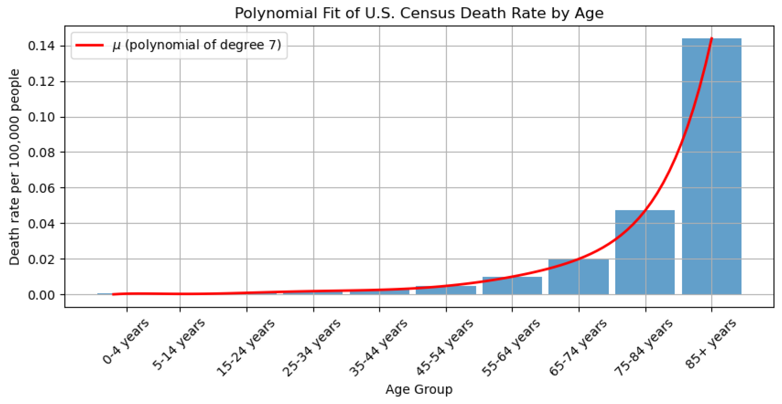
The death rate function $\mu$ is obtained by fitting the data with a polynomial of degree 7. The real death rate data and the graph of the polynomial are plotted in Figure 3.

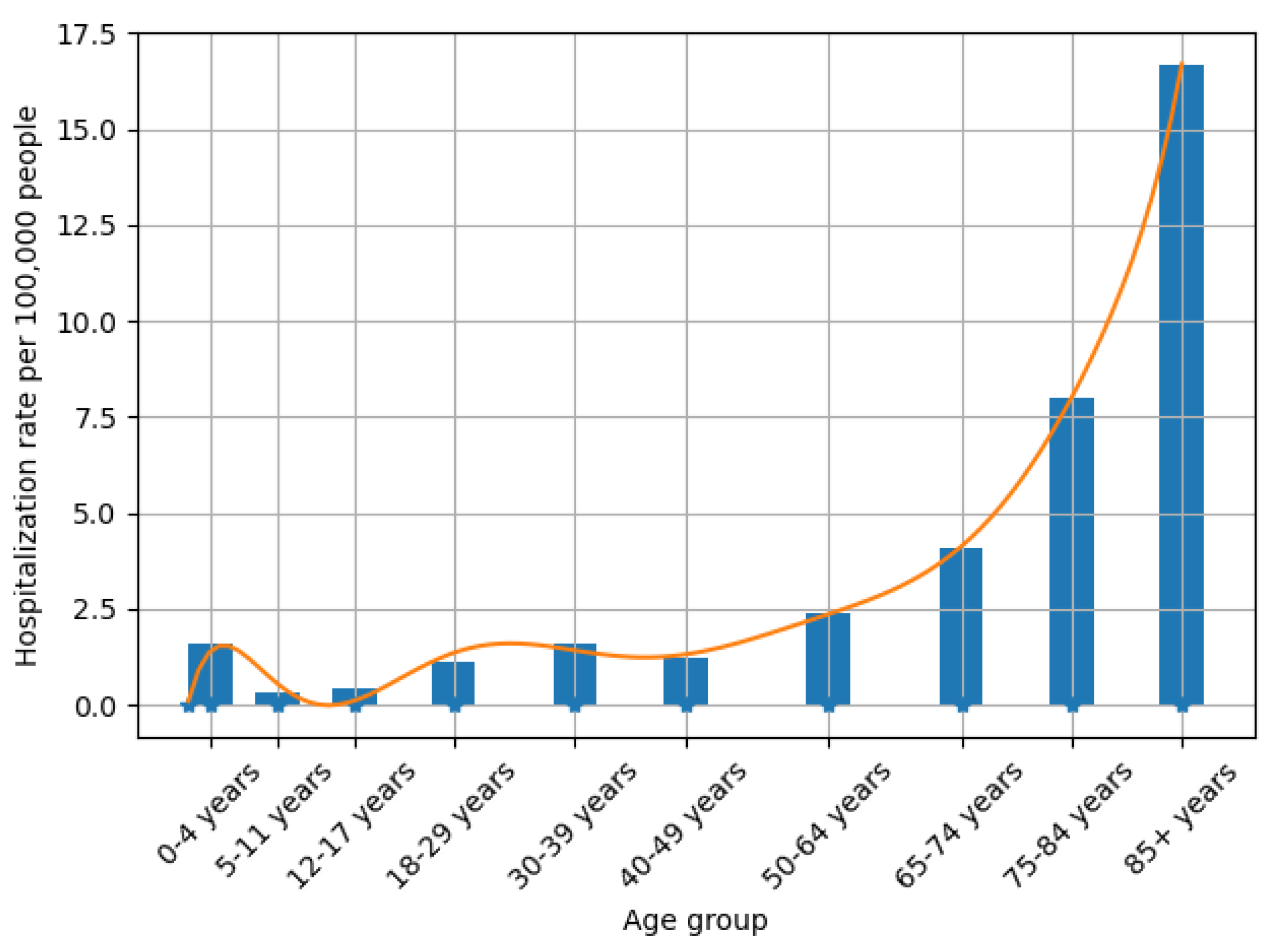
Similarly, the weekly hospitalization rate function $H_0$ is obtained by fitting a polynomial of degree 9 with the real data. Figure 4 shows the graph of $H_0$ and the data from the week of 2 April 2022. It is notable that the bars therein are not equidistant, as the age groups in the real data are not equidistant.

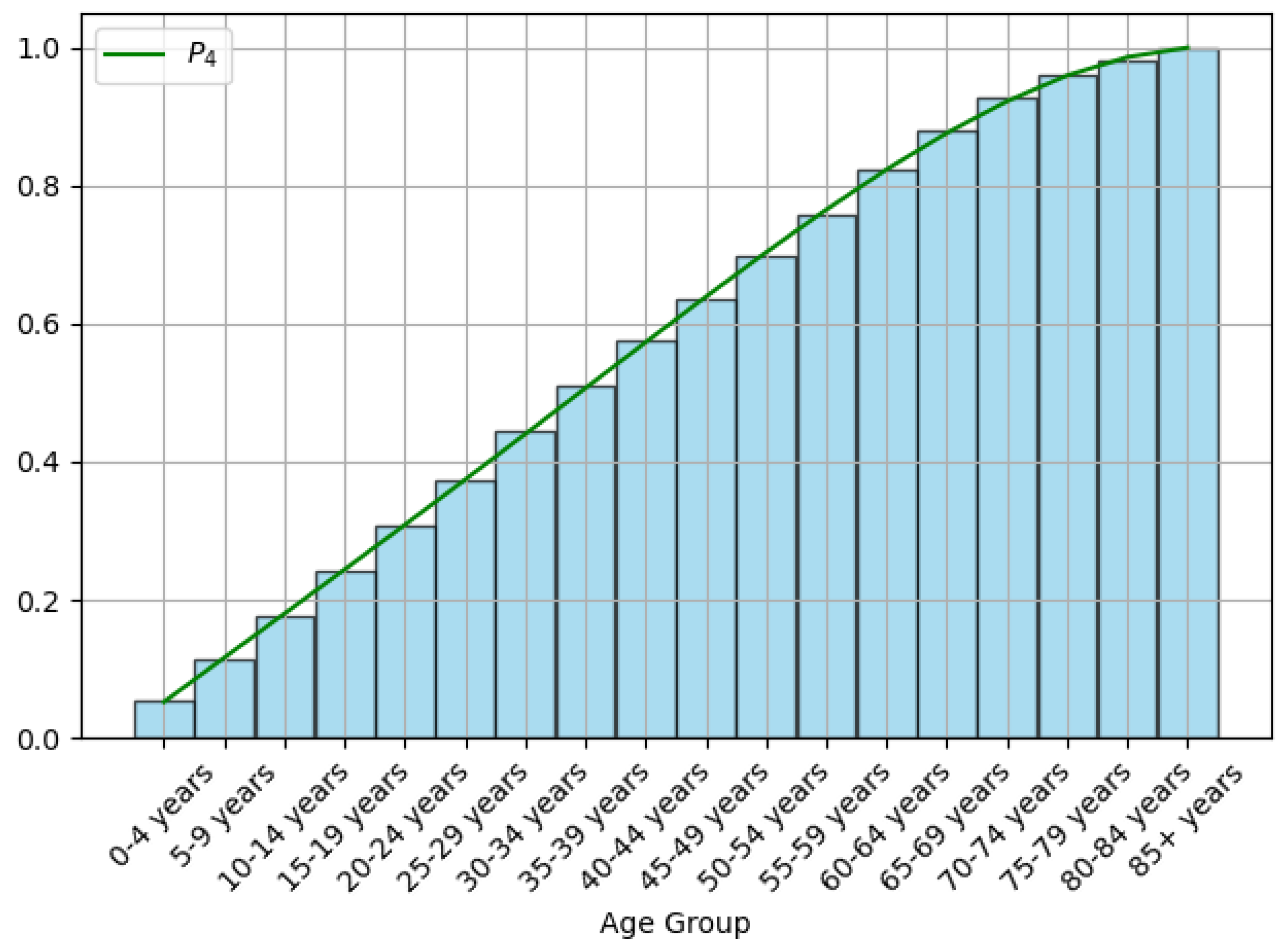
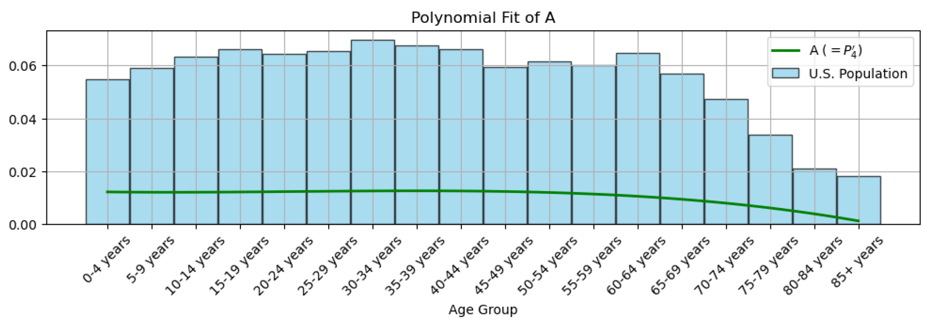
To approximate the density function, A, of the age distribution of the U.S. population, we first use a polynomial of degree 4, $P_4\left(a\right)$, to fit the cumulative age distribution. Then we have $A\left(a\right)=P_4^{\prime }\left(a\right)$ and $A^{\prime }\left(a\right)=P_4^{″}\left(a\right)$. The real data and the graph of $P_4$ are plotted in Figure 5. Figure 6 shows the age distribution of U.S. population and the graph of A.

Remark 2.

In the three interpolation tasks above, the polynomial degrees were not chosen arbitrarily. For each task, we tested interpolation polynomials of various degrees and selected the degree that provided the best overall fit to the underlying data trends while also satisfying the value constraint, e.g., ensuring that the age cumulative distribution remains between 0 and 1.

3.2. PINN Model Architecture

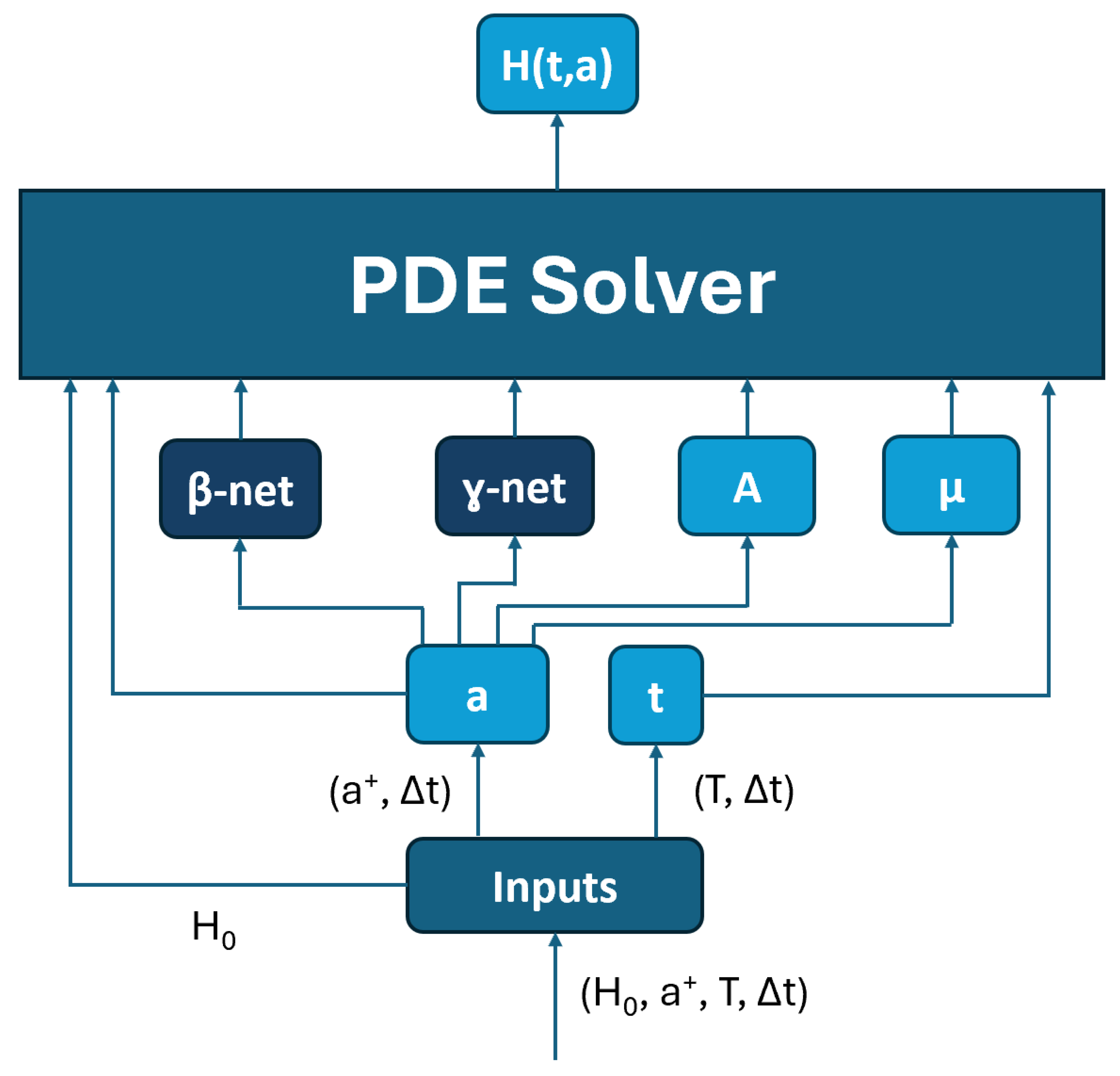
The PINN model uses $(H_0,a^{+},T,\Delta t)$ as the input, and outputs the predicted hospitalization rate $H(t,a)$, $0\le a\le a^{+}$, $0<t\le T$. Two sub-NNs, namely $\beta$-net and $\gamma$-net, are developed to approximate the functions $\beta$ and $\gamma$ in model (5), respectively. Then, a PDE-Solver layer is used to solve Model (5), (6) and output H. The PINN architecture is shown in Figure 7.

The roles of the blocks shown in Figure 7 are summarized below:

• The t block generates a discrete time interval ${[0,T]}_{\mathbb{Z}}:=\{0,\Delta t,2\Delta t,\dots ,T\}$ needed for other blocks based on the step size $\Delta t$ to discretize the time interval $[0,T]$.
• The a block discretizes the age interval $[0,a^{+}]$ as a discrete interval ${[0,a^{+}]}_{\mathbb{Z}}:=\{0,\Delta t,2\Delta t,\dots ,a^{+}\}$ needed for other blocks based on $\Delta t$.
• The A block and $\mu$ block calculate the needed values $A\left(a\right)$, $A^{\prime }\left(a\right)$, and $\mu \left(a\right)$ for $a\in {[0,a^{+}]}_{\mathbb{Z}}$, respectively.
• The $\beta$-net and $\gamma$-net approximate $\beta (a,\nu )$ and $\gamma \left(a\right)$, respectively. Both the $\beta$-net and $\gamma$-net utilize the residual network architecture, as illustrated in Figure 8.
• The PDE-Solver block numerically solves Model (5), (6) on the grid ${[0,T]}_{\mathbb{Z}}\times {[0,a^{+}]}_{\mathbb{Z}}$ using the method of characteristics, implemented with the Runge–Kutta method due to its high accuracy and stability for approximating ODE solutions. The reader is referred to [25] for the details of both methods.

It is notable that ${[0,T]}_{\mathbb{Z}}$ and ${[0,a^{+}]}_{\mathbb{Z}}$ share the same step size $\Delta t$, reflecting the fact that time t and age a progress at the same rate. This choice is also well-suited for applying the method of characteristics.

3.3. Forward Propagation Process

The forward propagation process of the PINN is to calculate $H(t,a)$, $0\le a\le a^{+}$, $0<t\le T$, by solving Model (5), (6) based on the input. The algorithm is summarized as Algorithm 1 below.

Algorithm 1 Forward propagation

1:  Initialize the PINN model with the model parameters $a^{+}$, T, the time step $\Delta t$, the census death rate function $\mu$, and the density function A for the age distribution of the U.S. population. Also, initialize the $\beta$-net and $\gamma$-net, and generate the grid $(t,a)\in {[0,T]}_{\mathbb{Z}}\times {[0,a^{+}]}_{\mathbb{Z}}$. 2:  Input the initial hospitalization rate $H_0$. 3:  For $t=\Delta t,2\Delta t,3\Delta t,\dots ,T$:    Set $H(t,0)=0$ and calculate $H(t,a)$, $a\in {[\Delta t,a^{+}]}_{\mathbb{Z}}$, based on $H(t-\Delta t,a)$, $a\in {[0,a^{+}-\Delta t]}_{\mathbb{Z}}$, along the characteristic lines. 4:  Output $H(t,a)$, $(t,a)\in {[0,T]}_{\mathbb{Z}}\times {[0,a^{+}]}_{\mathbb{Z}}$.

3.4. Training Process

Once the output H is calculated, the PINN is trained by minimizing the SE using the historical hospitalization data.

Let ${\tilde{H}}_i$ be the observed hospitalization rate at $(t_i,a_i)\in {[\Delta t,T]}_{\mathbb{Z}}\times {[\Delta t,a^{+}]}_{\mathbb{Z}}$, $i=1,2,\dots ,n$, and $\theta$ be the parameter vector that consists of all the NN parameters in $\beta$-net and $\gamma$-net. Then, the loss function L is defined by

$$\begin{array}{c}\hfill L\left(\theta \right)={\displaystyle \frac{1}{n}}\sum _{i=1}^n{e}^{min(t_i,a_i)/T}ln\left({(H(t_i,a_i;\theta )-{\tilde{H}}_i)}^2+1\right),\theta \in \mathrm{\Theta },\end{array}$$

(12)

where $\mathrm{\Theta }$ denotes the set of all possible $\theta$ values, and $e^{min(t_i,a_i)/T}$ represents a weight that emphasizes the errors of terms with longer evolution times. The goal of the training process is to find ${\theta }^{*}\in \mathrm{\Theta }$ such that

$$L\left({\theta }^{*}\right)=\underset{\theta \in \mathrm{\Theta }}{min}L\left(\theta \right).$$

Remark 3.

We would like to make the following remarks:

(1) 

Our model is primarily a classic finite-difference PDE solver for Model (5), (6), with two sub-NNs approximating β and γ. This choice ensures model interpretability and confines opacity to the sub-NNs. Numerical accuracy can also be guaranteed by classical numerical analysis.

(2) 

The optimization problem during the training process is solved using the Particle Swarm Optimization (PSO) algorithm [26] instead of traditional gradient-based ML training algorithms, as calculating gradients would be highly memory-intensive. The PSO algorithm enables us to train the model on a MacBook Pro laptop with 16 GB of memory.

(3) 

The PDE-Solver block can be implemented using alternative algorithms to enhance computational efficiency, including traditional numerical schemes or modern ML-based approaches. When ML-based methods are employed for solving PDEs, an additional physics-informed term must be incorporated into the loss function defined by (12) to compensate for the inherent opacity of NNs. In contrast, such a term is unnecessary for classical numerical solvers, as their error behavior is governed by the underlying numerical scheme.

(4) 

The sub-NNs, β-net and γ-net, can be implemented using other NN architectures instead of those shown in Figure 8, and can be trained using different algorithms given sufficient computational resources.

The training set contains 720 hospitalization rate records, randomly sampled from all age groups between 2 April 2022 and 24 August 2024, while the test set contains 180 observations, randomly sampled from the same period. The parameters of the PSO algorithm are given in

Table 2. Parameters for PSO Algorithm.

Swarm Size	20	Dimension of the Search Space	97
Maximum Number of Iterations	50	Search Space Bounds	${[-{\displaystyle \frac{\pi }{2}},{\displaystyle \frac{\pi }{2}}]}^{97}$
Cognitive Coefficient	2	Social Coefficient	1
Inertia Weight	0.5

.

3.5. Experiment Results

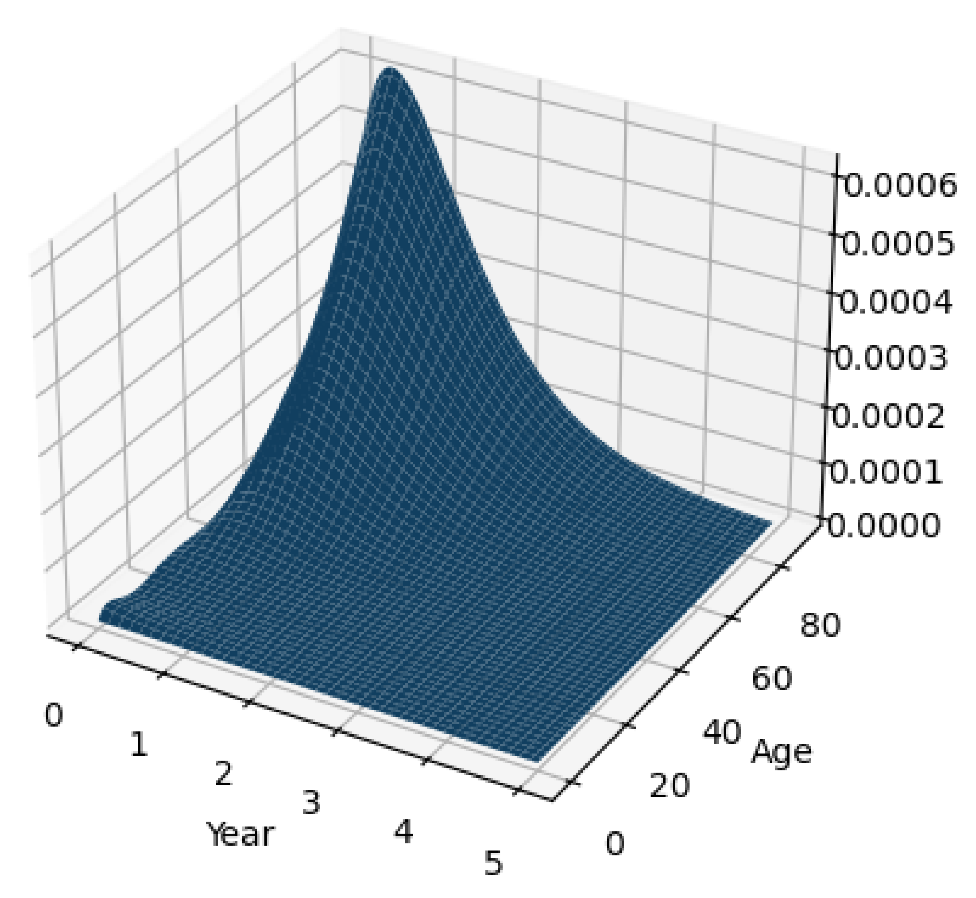
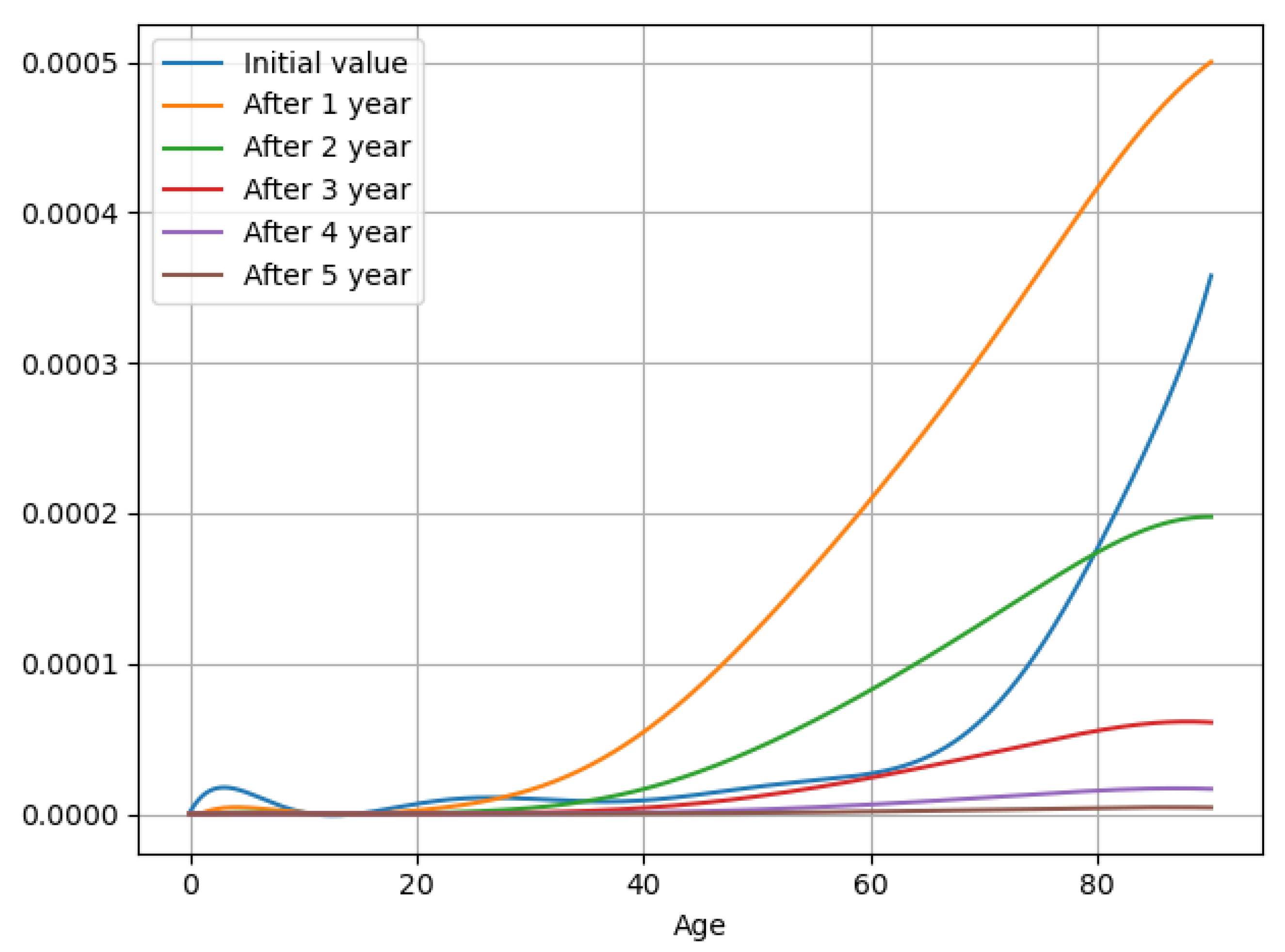
After training, the losses defined by (12) for the training set and the test set are $2.3445\times {10}^{-8}$ and $1.5006\times {10}^{-8}$, respectively. The trained model is then used to predict the hospitalization rate in the next 5 years using the data in the week of 24 August 2024. The experiment results are shown in Figure 9, Figure 10 and Figure 11.

The simulated results show a consistent trend for all age groups over time, and for any fixed time, the hospitalization rate increases with respect to age. This is consistent with observation during the outbreak of the pandemic—seniors are at higher risk compared to younger people with healthier immune systems.

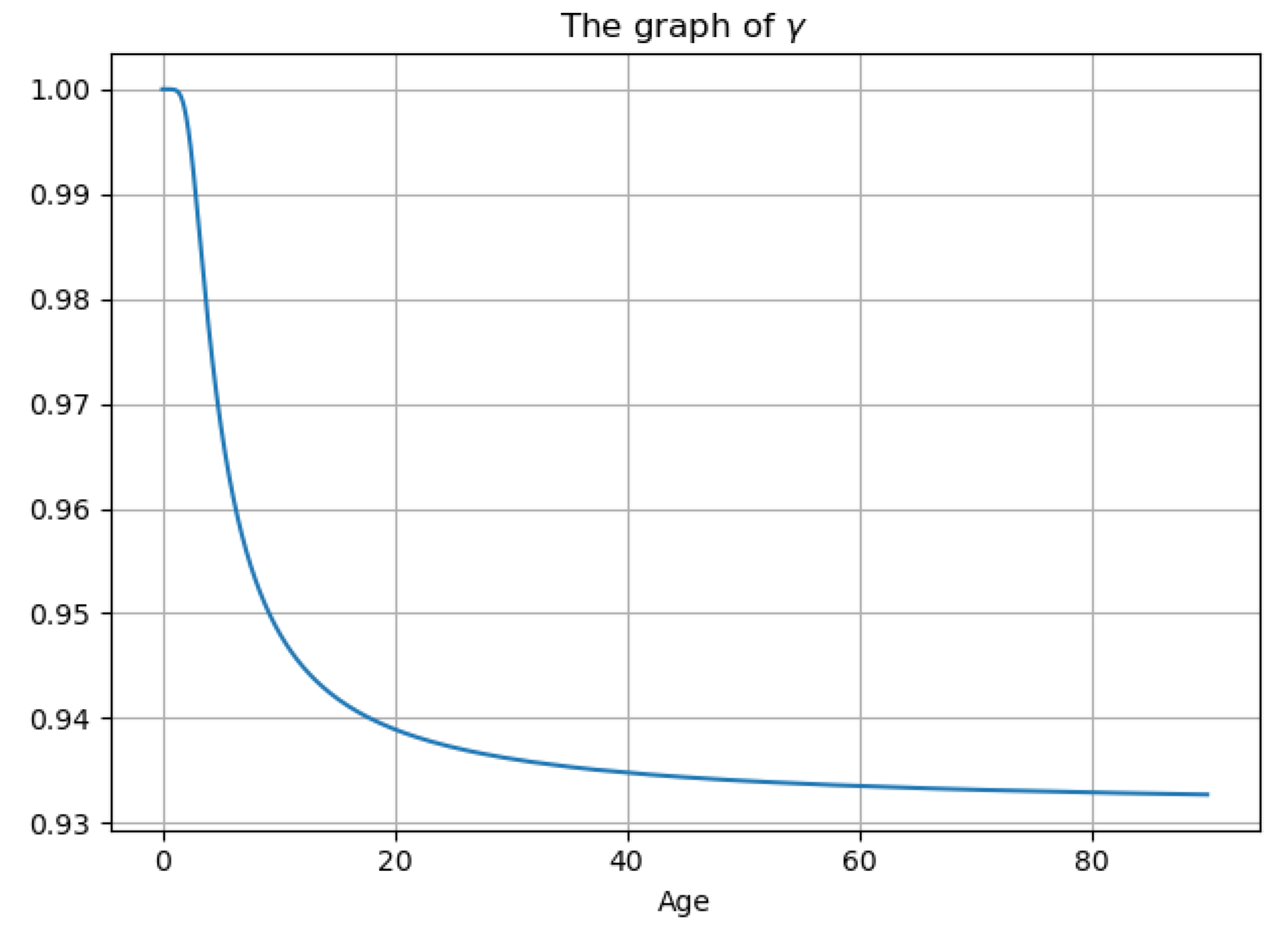
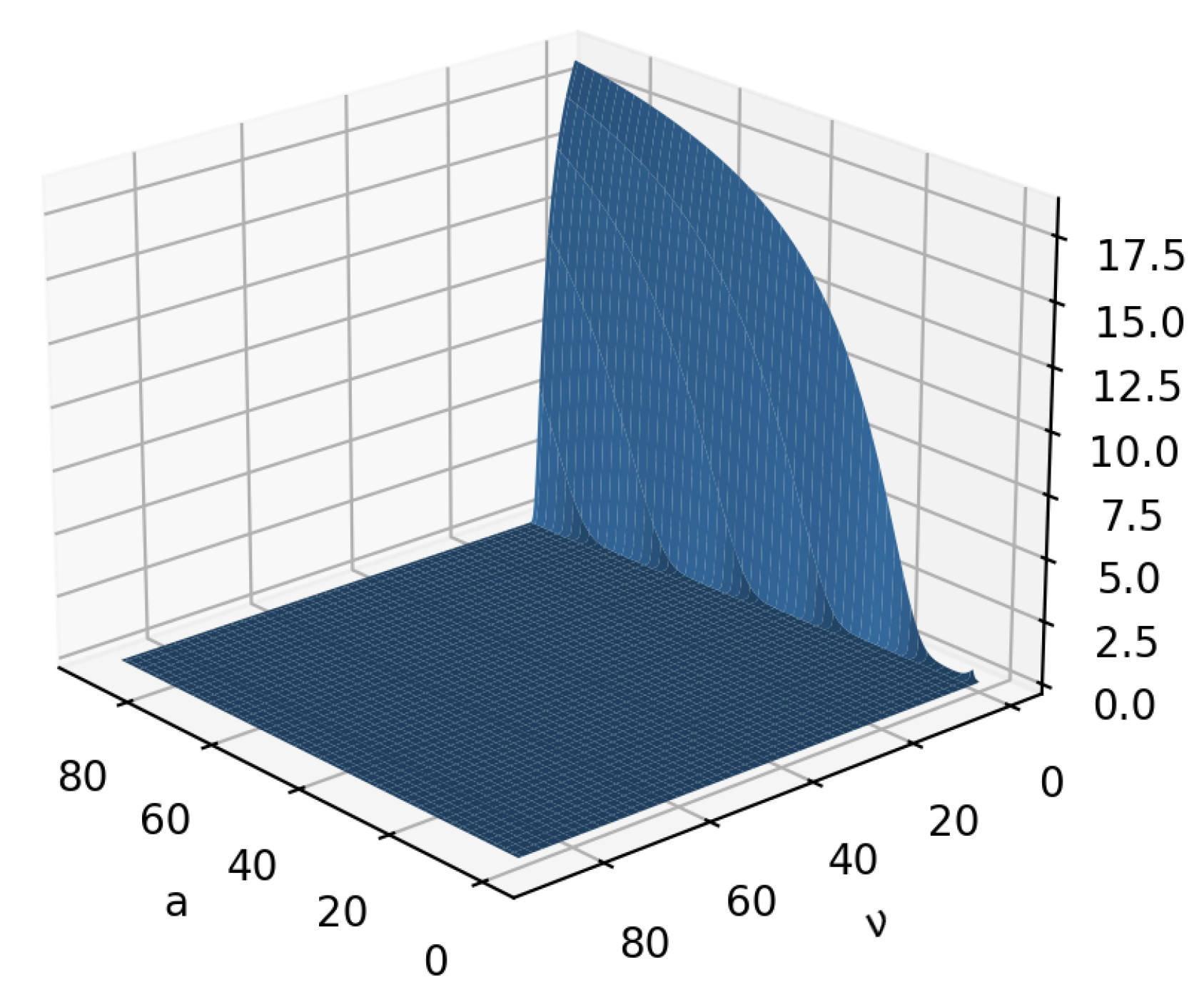
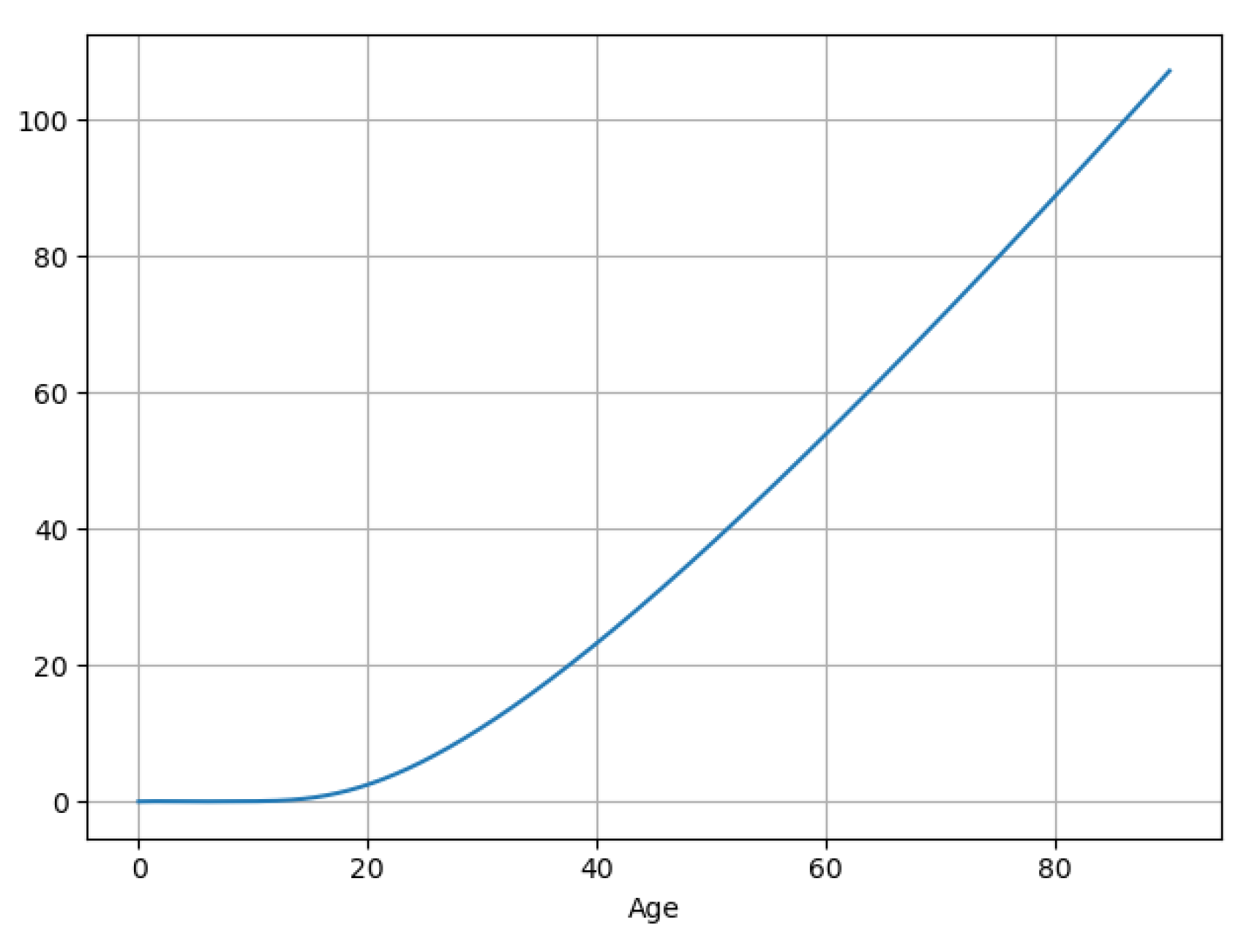
Since the $\beta$-net and $\gamma$-net in the PINN model are black boxes that are automatically determined during the training process, we also checked if the behavior of the trained networks was in agreement with our knowledge. The graphs of the fitted $\beta$ and $\gamma$ are also plotted in Figure 12, Figure 13 and Figure 14. In particular, Figure 12 shows that as age increases, the recovery rate of hospitalized patients decreases. While Figure 13 is less intuitive to interpret, Figure 14 plots the graph of ${\int }_0^{a^{+}}\beta (a,\nu )d\nu$, which represents the total impact of all age groups’ hospitalized populations on the population of age a, and this impact increases as a increases. These behaviors support our intuitive understanding that older people are more affected by the virus.

We further calculated

$$\underline{\eta }\simeq 0.6242607112791982\mathrm{and}{\beta }^{*}\simeq 18.550291$$

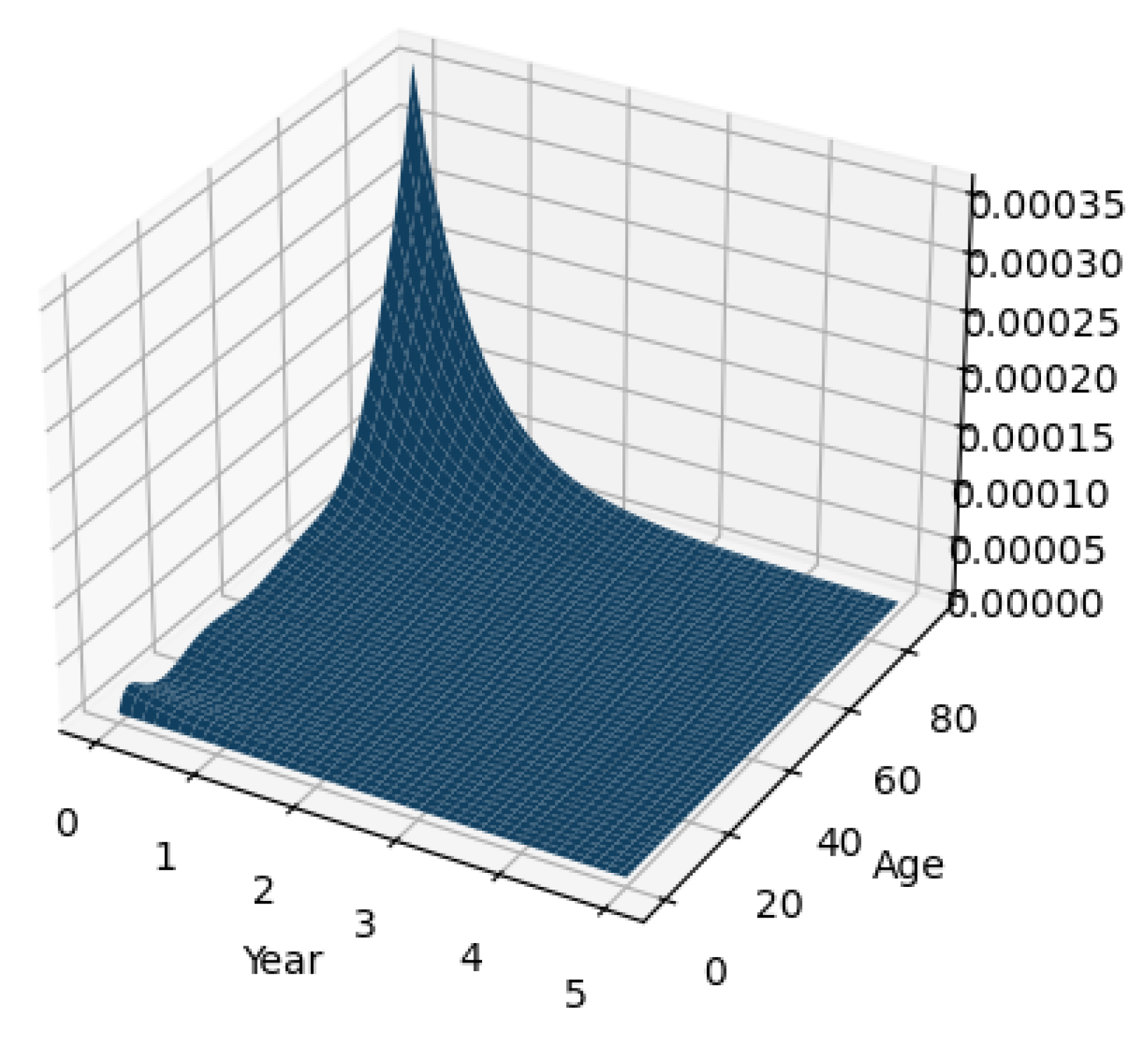
from the fitted $\beta$ and $\gamma$. By (11), we have $R_0>1$. We then manually decreased the values of $\beta$ by dividing $\beta$ by 100 so that the condition of Corollary 1 is satisfied, and carried out another round of experiments. The simulated result is plotted in Figure 15, which shows that the solutions are locally stable.

4. Conclusions and Discussion

In this paper, we developed an age-structured PDE model (5), (6), following a rigorous mathematical modeling procedure, to describe the post-pandemic COVID-19 hospitalization rate. Qualitative analysis was conducted to understand the properties of the mathematical model. Then a PINN model was designed based on (5). The PINN model was trained with real-world data, and the experiment results demonstrated superior performance.

This work used rigorous mathematical reasoning to guide the design of an ML model, and employed ML technologies to resolve computational challenges in traditional mathematical modeling. Therefore, it demonstrated the feasibility of combining the strengths of mathematical modeling with emerging ML technologies. This work also reveals some challenges. For example, the model assumptions were simplified so that the mathematical analysis could be conducted and the numerical experiment could be carried out with limited computing resources. In the future, we plan to develop new mathematical analysis techniques and ML solutions so that we can improve our model assumptions, to make the mathematical models better reflect reality.

References

1. Naseer, S.; Khalid, S.; Parveen, S.; Abbass, K.; Song, H.; Achim, M.V. COVID-19 outbreak: Impact on global economy. Front. Public Health 2023, 10, 1009393. [Google Scholar] [CrossRef] [PubMed]
2. Centers for Disease Control and Prevention. COVID Data Tracker; U.S. Department of Health and Human Services, CDC: Atlanta, GA, USA, 2024. Available online: https://covid.cdc.gov/covid-data-tracker (accessed on 29 October 2025).
3. National Flu and COVID-19 Surveillance Reports. UK Health Security Agency. Available online: https://www.gov.uk/government/statistics/national-flu-and-covid-19-surveillance-reports-2024-to-2025-season (accessed on 29 October 2025).
4. Surveillance and Updates on COVID-19. European Centre for Disease Prevention and Control. Available online: https://www.ecdc.europa.eu/en/covid-19/situation-updates (accessed on 29 October 2025).
5. Abernethy, G.M.; Glass, D.H. Optimal COVID-19 lockdown strategies in an age-structured SEIR model of Northern Ireland. J. R. Soc. Interface 2022, 19, 20210896. [Google Scholar] [CrossRef] [PubMed]
6. Ambalarajan, V.; Mallela, A.R.; Sivakumar, V.; Dhandapani, P.B.; Leiva, V.; Martin-Barreiro, C.; Castro, C. A six-compartment model for COVID-19 with transmission dynamics and public health strategies. Sci. Rep. 2024, 14, 22226. [Google Scholar] [CrossRef] [PubMed]
7. Brauer, F. Mathematical epidemiology: Past, present, and future. Infect. Dis. Model. 2017, 2, 113–127. [Google Scholar] [CrossRef] [PubMed]
8. Chen, S.; Shi, J.; Shuai, Z.; Wu, Y. Evolution of Dispersal in Advective Patchy Environments. J. Nonlinear Sci. 2023, 33, 40. [Google Scholar] [CrossRef]
9. ACiupeanu; Varughese, M.; Roda, W.C.; Han, D.; Cheng, Q.; Li, M.Y. Mathematical modeling of the dynamics of COVID-19 variants of concern: Asymptotic and finite-time perspectives. Infect. Dis. Model. 2022, 7, 581–596. [Google Scholar] [CrossRef] [PubMed]
10. Gao, D.; Yuan, X. A hybrid Lagrangian–Eulerian model for vector-borne diseases. J. Math. Biol. 2024, 89, 16. [Google Scholar] [CrossRef]
11. Iyaniwura, S.A.; Falcão, R.C.; Ringa, N.; Adu, P.A.; Spencer, M.; Taylor, M.; Colijn, C.; Coombs, D.; Janjua, N.Z.; Irvine, M.A.; et al. Mathematical modeling of COVID-19 in British Columbia: An age-structured model with time-dependent contact rates. Epidemics 2022, 39, 100559. [Google Scholar] [CrossRef] [PubMed]
12. Kiseleva, O.; Yakovlev, S.; Chumachenko, D.; Kuzenkov, O. Exploring Bifurcation in the Compartmental Mathematical Model of COVID-19 Transmission. Computation 2024, 12, 186. [Google Scholar] [CrossRef]
13. Ma, B.; Li, C.; Warner, J. Structured mathematical models to investigate the interactions between Plasmodium falciparum malaria parasites and host immune response. Math. Biosci. 2019, 310, 65–75. [Google Scholar] [CrossRef] [PubMed]
14. Ndaïrou, F.; Area, I.; Nieto, J.J.; Torres, D.F.M. Mathematical modeling of COVID-19 transmission dynamics with a case study of Wuhan. Chaos Solitons Fractals 2020, 135, 109846. [Google Scholar] [CrossRef] [PubMed]
15. Webb, G.; Zhao, X.E. An Epidemic Model with Infection Age and Vaccination Age Structure. Infect. Dis. Rep. 2024, 16, 35–64. [Google Scholar] [CrossRef] [PubMed]
16. Xiao, N.; Xu, H.; Morani, A.H.; Shokri, A.; Mukalazi, H. Exploring local and global stability of COVID-19 through numerical schemes. Sci. Rep. 2024, 14, 7960. [Google Scholar] [CrossRef] [PubMed]
17. Yu, Y.; Tan, Y.; Tang, S. Stability analysis of the COVID-19 model with age structure under media effect. Comp. Appl. Math. 2023, 42, 204. [Google Scholar] [CrossRef]
18. WHO Chief Declares End to COVID-19 as a Global Health Emergency. Available online: https://news.un.org/en/story/2023/05/1136367 (accessed on 29 October 2025).
19. Cuomo, S.; Cola, V.S.D.; Giampaolo, F.; Rozza, G.; Raissi, M.; Piccialli, F. Scientific Machine Learning Through Physics–Informed Neural Networks: Where we are and What’s Next. J. Sci. Comput. 2022, 92, 88. [Google Scholar] [CrossRef]
20. Hao, Z.; Liu, S.; Zhang, Y.; Ying, C.; Feng, Y.; Su, H.; Zhu, J. Physics-Informed Machine Learning: A Survey on Problems, Methods and Applications. arXiv 2023, arXiv:2211.08064. [Google Scholar] [CrossRef]
21. Kong, L.; Shi, R.Z.; Wang, M. A physics-informed neural network model for social media user growth. Appl. Comput. Intell. 2024, 4, 195–208. [Google Scholar] [CrossRef]
22. Zabczyk, J. Mathematical Control Theory: An Introduction; Birkhäuser: Cham, Switzerland, 1992. [Google Scholar]
23. The U.S. Census Bureau. Available online: https://data.census.gov/table/ACSST1Y2023.S0101?q=us%20age%20distribution (accessed on 29 October 2025).
24. Kochanek, K.D.; Murphy, S.L.; Xu, J.; Arias, E. Mortality in the United States, 2022. NCHS Data Brief No. 492. 2024. Available online: https://www.cdc.gov/nchs/products/databriefs/db492.htm (accessed on 29 October 2025).
25. Kincaid, D.; Cheney, W. Numerical Analysis: Mathematics of Scientific Computing, 3rd ed.; American Mathematical Society: Providence, RI, USA, 2002. [Google Scholar]
26. Zhang, Y.; Wang, S.; Ji, G. A Comprehensive Survey on Particle Swarm Optimization Algorithm and Its Applications. Math. Probl. Eng. 2015, 2015, 931256. [Google Scholar] [CrossRef]
Figure 1. Age-specific hospitalization rate over time.
Mathematics 14 00058 g001
Figure 2. Interactions among the cohorts.
Mathematics 14 00058 g002
Figure 3. Age-specific death rate function μ .
Mathematics 14 00058 g003
Figure 4. Age-specific hospitalization rate and H 0 .
Mathematics 14 00058 g004
Figure 5. Cumulative age distribution and P 4 .
Mathematics 14 00058 g005
Figure 6. Age distribution and A.
Mathematics 14 00058 g006
Figure 7. The PINN architecture.
Mathematics 14 00058 g007
Figure 8. (a) Architecture of β -net, x R 2 . (b) Architecture of γ -net, x R .
Mathematics 14 00058 g008
Figure 9. The simulated COVID-19 hospitalization rate in 5 years.
Mathematics 14 00058 g009
Figure 10. The simulated COVID-19 hospitalization rates at various time points.
Mathematics 14 00058 g010
Figure 11. The simulated COVID-19 hospitalization rates for various age groups.
Mathematics 14 00058 g011
Figure 12. The graph of γ .
Mathematics 14 00058 g012
Figure 13. The graph of β .
Mathematics 14 00058 g013
Figure 14. The graph of 0 a + β ( a , ν ) d ν .
Mathematics 14 00058 g014
Figure 15. The simulated result when the conditions of Corollary 1 are satisfied.
Mathematics 14 00058 g015