Article

Efficient Multiple Path Coverage in Mutation Testing with Fuzzy Clustering-Integrated MF_CNNpro_PSO

1
School of Information Engineering, Yancheng Institute of Technology, Yancheng 224051, China
2
School of Information Engineering (School of Big Data), Xuzhou University of Technology, Xuzhou 221018, China
*
Author to whom correspondence should be addressed.
Mathematics 2026, 14(1), 47; https://doi.org/10.3390/math14010047
Submission received: 20 October 2025 / Revised: 12 December 2025 / Accepted: 18 December 2025 / Published: 23 December 2025

Abstract

Fault concealment in complex software programs and the difficulty of generating test cases to detect such faults present significant challenges in software testing. To resolve these challenges, this paper suggests a novel method that integrates mutation testing, fuzzy clustering, convolutional neural networks (CNN), and particle swarm optimization (PSO) to efficiently generate test cases that cover multiple paths with numerous faults (mutant branches). Initially, mutation-based paths are classified using fuzzy clustering based on their coverage difficulty and similarity. A multi-feature CNN model (MF_CNNpro) is then constructed and trained on the paths of each cluster. Finally, the predicted particles from the MF_CNNpro model are used as the initial population for PSO, which evolves to generate the test cases. The proposed method is evaluated on six test programs, and the results demonstrate that it significantly improves clustering separation and reduces clustering compactness. By selecting only the cluster center paths to construct the MF_CNNpro model, training and prediction costs are effectively reduced. Moreover, the use of MF_CNNpro and PSO to select representative individuals as the initial population greatly enhances the evolutionary efficiency of PSO. The proposed method outperforms traditional approaches in clustering, prediction, and test data generation. Specifically, the SC clustering method improves cluster separation (SP) by 0.021, reduces compactness (CP) by 0.054, and decreases clustering rate (CR) by 4.97%, thereby enhancing clustering precision. The MF_CNNpro model improves the IA metric by 38.2% and reduces the U-Statistic and MSE by 83.0% and 97.9%, respectively, optimizing prediction performance. The MF_CNNpro+PPSOpro method increases the path coverage success rate from 47.9% to 97.4% (a 103.3% improvement), reduces the number of iterations by 84.1%, and decreases execution time by 95.6%, significantly improving generation efficiency.

1. Introduction

Software testing aims to verify that the software meets specified requirements, identify faults to reduce their impact, and evaluate software quality [1]. Mutation testing is a fault-oriented technique within software testing. It involves injecting artificial faults (mutants) and assessing whether existing test cases can detect these faults, thereby evaluating the adequacy of the test case design [2]. The primary goal of mutation testing is to make test cases more effective. Many stubborn faults are difficult to detect using traditional testing methods, and designing test cases to detect them is also important [3]. Therefore, this paper aims to generate test cases targeting hard-to-detect faults based on mutation testing, using convolutional neural networks (CNN) [4] and the particle swarm optimization algorithm (PSO) [5]. By using these “enhanced test cases” in software testing, real faults can be discovered more efficiently, with one study showing a 51.6% relative improvement in the rate of fault detection [6].
In general, mutation testing is categorized into two types: “weak mutation testing” and “strong mutation testing”  [7,8]. Weak mutation testing sacrifices the strict requirement of strong mutation on output differences but achieves lower computational costs, simpler execution processes, and faster feedback. In practical applications, weak mutation testing is more suitable as a preliminary evaluation tool for test cases, especially in large software systems or complex code modules, where it can quickly detect difficult-to-cover faults at a relatively low cost [9]. Therefore, this paper primarily focuses on weak mutation testing techniques.
Papadakis et al. [10]. proposed the concept of the “mutant branch.” A mutant branch essentially transforms the “necessary conditions” of weak mutation into an efficiently executable code structure. Mutant branches help reduce the overhead of strong mutation testing. Additionally, Zhang et al. [11]. employed branch coverage testing inside the context of well-established  structural coverage, transforming the weak mutation problem toward a branch coverage issue. But their method resulted in redundant test data due to the correlation between mutant branches. Notably, the use of a large number of mutant branches in a program can lead to issues such as code bloat and reduced execution efficiency. Therefore, this paper focuses on addressing these problems caused by mutant branches.
As in our previous reach [12], mutant branches can be transformed into mutation-based paths using the correlation between mutant branches and applied to MPI (Message-Passing Interface) parallel programs. Tao et al. [13] proposed a method based on bidirectional traversal of correlation graphs, grouping mutant branches by path. These mutation paths only contain mutant branches. By covering a mutation path with a test case, multiple mutant branches along the path are also covered, which helps reduce the size of the generated test set. However, due to the significant code bloat caused by mutant branches, the number of generated mutation paths remains large. To address this, this paper applies a fuzzy clustering method to group mutation paths, treating multiple similar paths within the same cluster as a single task for processing.
In recent years, evolutionary algorithms such as Genetic Algorithm (GA), Particle Swarm Optimization (PSO), and Ant Colony Optimization (ACO) have been widely applied in the field of test case generation, achieving significant results [14,15]. PSO, in particular, has gained considerable attention due to its advantages of simple implementation, fast convergence, and strong versatility [16]. In the field of software testing, the “strong versatility” of PSO refers to its ability to be independent of specific testing scenarios, program types, or optimization objectives [17]. It can be flexibly adapted to various software testing tasks and complex scenarios without requiring extensive customization for specific test subjects. This aligns with the practical application scenarios in software testing, such as test case generation, path coverage, fault localization, and others. Allawi introduced a novel hybrid algorithm combining greedy methods and PSO (GPSO), ensuring the effectiveness of generating the minimum number of test cases while delivering results close to the optimal [18]. Ojdanić proposed a multi-path test case generation method based on metamorphic relations (MRs), significantly improving efficiency in terms of fitness evaluation and time consumption [15]. Boukhlif developed an adaptive PSO-based optimization algorithm for software testing that dynamically adjusts the inertia weight based on iteration progress and average relative speed, effectively addressing issues such as population diversity loss and low local search accuracy, thus enhancing PSO performance [14].
Evolutionary algorithms generate high-quality test cases by simulating the process of biological evolution. However, one of the core bottlenecks causing algorithm inefficiency is that “evolutionary individuals frequently execute the program under test to calculate their fitness” [19,20]. This becomes especially problematic when the program under test is complex or time-consuming or when the population size is large, potentially leading to a “computational explosion”. Machine learning, with its ability to learn patterns from data and model complex relationships, provide targeted solutions to address this bottleneck in evolutionary algorithms [21,22].
A surrogate model based on machine learning can learn the approximate behavior of a target function (fitness function) based on existing sample data [13]. In evolutionary algorithms, surrogate models can be used to estimate the fitness values by replacing the actual target function. Commonly used surrogate models are the Backpropagation Neural Network (BP), radial basis function networks (RBFN), and convolutional neural networks (CNNs) [23,24,25].
Yao et al. [26] were among the first to propose using BP Neural Networks as surrogate models to optimize evolutionary algorithms in test case generation. Their approach begins by randomly generating initial data (evolutionary individuals), executing the program under test, and calculating the true fitness values of these individuals. This initial data, along with the corresponding fitness values, is then used to construct a sample set for training the neural network. The neural network model is subsequently employed to estimate the fitness values of the individuals. Finally, individuals with high estimated fitness values are selected to execute the program under test, where their true objective function values are computed, thereby reducing the execution cost of the evolutionary algorithm.
Building on this method, Tao Lei et al. [13] proposed an enhanced convolutional neural network (CNNpro) model to optimize evolutionary algorithms. Both CNN and CNNpro are fully capable of serving as surrogate models for path coverage. CNN, through the local receptive field and parameter-sharing mechanism of convolutional kernels, automatically extracts hierarchical structural features of paths (such as branch dependencies and coverage pattern differences). This enables the precise capture of the intrinsic relationship between path structure and coverage effectiveness, making it highly efficient in meeting the surrogate model requirements for path coverage and facilitating the accurate prediction of adaptive values.
However, traditional CNNs and CNNpro construct surrogate models for a single path and can only generate a single output feature. This limitation results in significant computational resource consumption when separate models need to be built and trained for multiple paths, leading to poor model reusability. To address this issue, this paper draws on the CNNpro model [13] and proposes the Multi-dimensional Feature Convolutional Neural Network (MF_CNNpro) model. By incorporating multi-dimensional output features, the MF_CNNpro model is able to simultaneously capture three complementary test adequacy features. Furthermore, the proposed method directs the output features based on the positional differences between paths, allowing multiple paths to share a single model. This overcomes the limitation of single-path models (CNN), reduces the cost of redundant model construction, and maintains the model’s effectiveness in predicting different paths by capturing “differential features,” thereby enhancing its generalizability.
In light of the aforementioned analysis, to increase the effectiveness of generating test cases for a large number of mutation paths and enhance the error detection capability of the test cases, this paper utilizes fuzzy clustering methods to group numerous mutation paths. For each cluster, a multi-dimensional feature-enhanced convolutional neural network (MF_CNNpro) is constructed and trained based on the similarities and differences among the paths. Subsequently, MF_CNNpro estimates the high-fitness particles for the initial population. Finally, an improved algorithm of the hypercube boundary value particle swarm optimization (improved PSO) is employed to generate test data, thereby enhancing the global search capability. The proposed method makes significant contributions in three main aspects:
  • Fuzzy Clustering for Path Grouping: This method groups mutation-based paths into the same cluster based on their similarity while allowing a single path to belong to multiple clusters. The fuzzy clustering approach more accurately reflects the real-world relationships between paths, where the boundaries of path similarity are often ambiguous and categories may overlap.
  • Enhanced MF_CNNpro Model Construction with Multi-Feature Integration for Improved Prediction Accuracy: A MF_CNNpro model is constructed for each cluster, rather than for each path within the cluster, significantly reducing the cost of constructing and training surrogate models. In the model, the input features are the program’s inputs, while the traversal path serves as an auxiliary feature, enriching the model with additional diversity information. The output consists of three features. In addition to fitness as a feature (as in traditional models), two extra features are introduced, highlighting the differences between other paths and the center path. This design enables the model to generate differentiated predictions even when different paths share the same fitness value, addressing the “single-value confusion” problem common in traditional models. As a result, the model enhances both the discriminability and practical value of the prediction results.
  • Efficient Test Case Generation via MF_CNNpro Reuse and PSO for Cross-Path Collaboration: A single MF_CNNpro model for each cluster can estimate high-fitness particles for multiple paths as initial particles in the particle swarm. The “one-time modeling, multiple reuse” mechanism significantly improves the model’s efficiency. If a generated particle fails to provide optimization value for a current target path, it can be evaluated to determine whether it is useful for other paths within the cluster. This strategy reduces the number of redundant predictions. By efficiently reusing the MF_CNNpro model and facilitating cross-path collaboration during the particle swarm iteration, this approach ensures prediction accuracy while significantly improving the efficiency of test case generation. Additionally, improved PSO utilizes a hypercube to define the search space and guides the particle search by handling boundary values, thereby preventing particles from getting trapped in local optima.
The three techniques (Fuzzy Clustering, MF_CNNpro, and PSO) work in a progressive and synergistic manner, addressing the complexity of the path coverage problem hierarchically and enhancing efficient mutation test case generation.

2. Background

2.1. Mutation-Based Path

“Mutation-based path” is defined as a path formed exclusively by mutant branches. “Mutant branch” is constructed by the original and mutated statement according to the essential conditions for mutation testing [1]. The rationale for constructing mutant branches is as follows: strong mutations are transformed into weak mutations to identify all possible mutations of the tested statement (based on mutation operators such as operator replacement, variable substitution, etc.). These mutated logic conditions are inserted into the original program as conditional branches, with a mutation flag controlling which version of the mutation to execute. A single run can cover the logic of all mutated versions, and by analyzing the intermediate state differences under different branches, it enables the simultaneous validation of multiple mutants.
Considering the large number of mutant branches within the program being tested, Tao et al. [13] proposed a two-way traversal method using graph theory to produce a set of mutation-based paths. The mutation-based path clustering problems discussed in this paper are based on the paths obtained using the method proposed by Tao et al. [13].
The main steps of their method are as follows: First, a mutant branch correlation graph is constructed based on the relationships between the mutant branches. Then, from the mutant branch set M = { M 1 , M 2 , , M m } , the mutant branch with the highest coverage difficulty, M i , is selected as the benchmark node for path construction, and  M i is placed in the mutant branch correlation graph. Using this benchmark node as the starting point, the first direction of traversal is along the successor direction. The most highly correlated successor node is added to the path. The current node is updated, and the next node with the highest correlation is selected. If there is no conflict with any node in the path, it is included; otherwise, it is skipped, and the next one is considered. The second direction is the predecessor direction for traversal. It efficiently generates a set of paths that cover the mutant branches while minimizing the test set size, improving the efficiency of mutation testing.

2.2. Test Data Generation Using Evolutionary Algorithms

In software testing, the process of generating coverage path test data using evolutionary algorithms involves simulating the biological evolution mechanisms of “selection, crossover, and mutation.” This approach efficiently searches within the input data space to identify test cases that trigger specific program paths, such as branch or path coverage.
The construction of the mathematical model essentially transforms path coverage into a numerical optimization problem. This is followed by an iterative framework of “population initialization, fitness evaluation, evolutionary operator, update termination condition check.” The core challenge lies in the rationality of the fitness function (whether it can accurately reflect the degree of proximity to the target path) and the tuning of operator parameters (whether it can balance exploration and exploitation). Therefore, a flexible design, tailored to the path characteristics of the specific program, is required.
In software testing, generating test case using evolutionary algorithms involves simulating the biological evolution mechanisms of “selection, crossover, and mutation.” This approach efficiently explores the input data domain to identify test cases that activate specific program paths, such as branch or path coverage.
The mathematical model is constructed by transforming path coverage into a numerical optimization problem. This is followed by an iterative framework consisting of “population initialization, fitness evaluation, evolutionary operator, update termination condition check.” The core challenge lies in the rationality of the fitness function (i.e., whether it can accurately reflect the proximity to the target path).
After executing the initial data X through the program, the combination of nodes covered by X from the program’s start to the end forms a traversal path g ( X ) . The similarity between the traversal path g ( X ) and the target path S i is then defined as the objective function f i ( X ) for coverage path test data. The traversal path g ( X ) is more comparable to the target path S i when f i ( X ) is higher. X covers S i when f i ( X ) = 1 , which means that S i is the same as g ( X ) .
For the target path S i , we can transform the test data generation for the path coverage problem into a maximization problem, i.e.,  max   f i ( X ) . The mathematical model for the test data generation for covering path S i can be expressed as
max f i ( X ) s . t . X D
where D is the domain of input variables. Thus, based on the objective function for S i , the fitness function is defined as
F i t n e s s i ( X ) = f i ( X )

2.3. Convolutional Neural Networks (CNNs)

Convolutional Neural Networks (CNNs) are a commonly used type of deep learning network. In the fields of software engineering and software testing, CNNs are primarily applied due to their powerful feature extraction and pattern recognition capabilities. They are used in code defect detection and vulnerability identification by converting code into matrix representations to learn defect patterns.
In the path coverage testing experiments, Tao et al. [13] compared CNN with other neural network models such as DNN (Deep Neural Network), LSTM (Long Short-Term Memory), and RNN (Recurrent Neural Network). The comparison was based on four classical metrics: IA (Information Accuracy), U-Statistic, MSE (Mean Squared Error), and memory consumption (MiB). These metrics provide a comprehensive evaluation of the models from multiple perspectives, including accuracy, generalization ability, resource usage, and computational efficiency. Experimental validation shows that CNN not only increased the accuracy of the predictive model but also improved the efficiency of test data generation.
Pan et al. [27] applied Convolutional Neural Networks (CNNs) to regression testing with the aim of reducing costs. A more recent study by Chen et al. [28] demonstrated the ability of CNNs to analyze program structures and predict testing adequacy. The approaches proposed by Pan et al. and Chen et al. often overlook the execution context, such as traversal paths, which limits their ability to model the relationship between program inputs and path coverage. To address this limitation, Tao et al. introduced the CNNpro model. This modification enhances the model’s ability to capture program behavior patterns, thereby improving prediction accuracy. Furthermore, they employed sequential incremental learning techniques (SI_CNNpro) to dynamically update the model in real time, which helps refine the sample set.
However, the CNNpro model is limited by being designed for a single path and generating only a single output feature, which results in poor model reusability. This paper improves upon the CNNpro technique by capturing three output features and developing a multi-path model that can be applied to a broader range of paths.

3. The Proposed Method

Figure 1 illustrates the three-stage execution framework of the proposed method, which efficiently generates test cases through a “clustering-modeling-generation” workflow based on mutation paths:
Stage 1: Mutation Path Clustering via Fuzzy Clustering
The first stage involves clustering mutation paths using fuzzy clustering. This step reduces the large volume of mutation paths by leveraging “path difficulty” and “inter-path similarity” as key features. The input is the original set of mutation paths, which includes numerous fault-associated paths. The fuzzy clustering technique groups paths into clusters based on feature similarity (instead of hard partitioning), thus addressing the issue of excessive path count while maintaining the fuzzy nature of path similarity. The output is a set of path clusters, labeled “Cluster 1, …, Cluster n” in the figure.
Stage 2: Model Construction using MF_CNNpro
The second stage constructs the MF_CNNpro model based on the center paths of each cluster identified in the previous stage. For each cluster, a dedicated MF_CNNpro model is trained using the paths within the cluster. The model is constructed by analyzing the similarities and differences among paths, combining multi-dimensional path features, and using the center path as a reference to define the model’s input/output structure and training parameters. The output is an MF_CNNpro model corresponding to each cluster.
Stage 3: Test Case Generation using MF_CNNpro and PSO
The final stage generates test cases using the MF_CNNpro model and Particle Swarm Optimization (PSO). This combination enables cross-path collaborative test case generation. The process involves selecting initial particle swarms with high coverage potential from the MF_CNNpro model of the corresponding cluster and using PSO’s global search capability to avoid local optima. This collaborative approach allows for test case generation that spans multiple paths within a cluster. The output is a high-quality test case set for the corresponding cluster.
This layered framework, which first streamlines paths via clustering, then models each cluster, and finally generates test cases collaboratively, addresses the challenge of excessive mutation paths. It also enhances the efficiency and coverage of test case generation by integrating cluster-specific models and PSO.

3.1. Mutation-Based Path Clustering Using Fuzzy Clustering

A mutation-based path is defined as one that is formed exclusively by mutant branches.
Let P be the program under test with inserting some mutant branches. A set of mutant branches M = { M 1 , M 2 , , M m } , where m represents the number of branches.
The set of mutation-based paths is obtained based on the literature.
The complexity of the mutant branches determines the difficulty of mutation-based path coverage. The operators used within the mutant branches, such as arithmetic, logical, and bitwise operators, along with the number of operands, serve as indicators for assessing the difficulty of these branches [29]. An increase in the number of operators and operands may result in greater computational complexity and heightened difficulty in understanding the mutant branches.
Thus, the difficulty of a mutation-based path is determined based on the following four principles:
  • The number of mutant branches included in the path.
  • The number of operators and operands involved in the path.
  • The density of operators within the path, where the presence of multiple operators in the same expression increases complexity.
  • The number of special operators, such as ternary operators, lambda functions, and regular expression metacharacters, which increase the complexity of the path.
Next, the paths are ranked according to the four principles mentioned above. After sorting, an ordered set of paths is obtained, S = { S 1 , S 2 , , S n } , where n represents the total number of paths. The first path S 1 corresponds to the most difficult path to cover.
Let two different paths be S i and S j , where i , j = 1 , 2 , , n , and  i j . | S i | and | S j | denote the lengths of the two paths, corresponding to the number of mutant branches contained in each path. The similarity between S i and S j is denoted as i , j , where
i , j = | S i S j | max | S i | , | S j |
In Equation (3), i , j [ 0 , 1 ) , where | S i S j | represents the number of common mutant branch nodes between S i and S j , and  max | S i | , | S j | represents the maximum path length.
Note that the path similarity method in this paper differs from that in the study by Tao et al. [13]. In Equation (3), we set the numerator as the total number of identical nodes between the two paths, rather than the “number of consecutive identical nodes starting from the initial position of the two paths” used by Tao et al. [13]. The reason for this adjustment is that mutation-based paths only include mutant branches, so a higher similarity can still be indicated even if the initial nodes differ, as long as there is a greater overlap in the latter half of the paths.
Furthermore, choosing max ( | S i | , | S j | ) over the minimum or average is reasonable and significant for clustering overlap.
1. Rationale for Selecting max ( | S i | , | S j | )
In mutation testing, the primary objective of path similarity measurement is to reflect the overlap of mutation branches covered by paths, as branch coverage directly correlates with fault detection capability. Selecting max ( | S i | , | S j | ) as the denominator in the similarity metric i , j = | S i S j | max ( | S i | , | S j | ) is both theoretically and practically motivated by its alignment with the coverage-oriented goals of mutation testing, ensuring semantic rationality, robustness, and interpretability.
Below, we provide a detailed comparison with the use of the minimum or average of path lengths:
(1) Alignment with Coverage-Centric Semantics in Mutation Testing
Path similarity in mutation testing aims to quantify the degree to which two paths share mutant branches, and thus, their fault-detection patterns. By using max ( | S i | , | S j | ) , the number of shared branches is normalized by the length of the longer path (the more comprehensive path), which inherently measures the proportion of the longer path’s mutant branches covered by the shorter path. A similarity value of 1 is achieved only if the shorter path is a complete subset of the longer path, and all branches of the shorter path are contained within the longer one—this aligns directly with the semantic requirement of similar coverage capability.
Example: Let S i = M 1 , M 2 , M 3 (length 3, covering 3 mutant branches) and S j = M 1 , M 2 (length 2, covering 2 mutant branches), with  | S i S j | = 2 . Using max ( | S i | , | S j | ) = 3 , the similarity is 2 3 0.67 , which accurately reflects that “ S j covers only 67% of S i ’s mutation branches,” avoiding overestimation of their fault-detection consistency. In contrast, using min ( | S i | , | S j | ) = 2 results in a similarity of 1, falsely implying identical coverage capabilities. This misalignment is critical in mutation testing, where path length is often indicative of fault-detection scope.
(2) Avoiding Misleading Similarity Inflation for Asymmetric Path Lengths (vs. Minimum)
When paths have significantly different lengths, using the minimum length as the denominator artificially inflates the similarity, leading to erroneous clustering of paths with disparate fault-detection capabilities.
Example: Let | S i | = 10 (a long path covering 10 critical mutation branches) and | S j | = 3 (a short path covering 3 branches, all of which are subsets of S i ). Using min ( | S i | , | S j | ) = 3 results in a similarity of 1, misleadingly suggesting identical fault detection potential. However, S j only covers 30% of S i ’s mutation branches, and its fault-detection range is substantially narrower. In contrast, using max ( | S i | , | S j | ) = 10 yields a similarity of 3 10 = 0.3 , which accurately reflects the “partial coverage” nature of S j . This prevents the misclassification of “the shorter path being a subset of the longer path” as “path similarity,” ensuring that clustering groups paths with proportionally high branch overlap.
(3) Ensuring Interpretability and Stability (vs. Average)
The average of path lengths, i.e.,  | S i | + | S j | 2 , lacks clear semantic meaning and produces ambiguous results, which undermines the academic rigor of the metric.
Example: Continuing with S i (length 3) and S j (length 2), the average length is 2.5, resulting in a similarity of 2 2.5 = 0.8 . This value lies between the minimum-based (1.0) and maximum-based (0.67) results but cannot be interpreted as a “coverage ratio.” It does not represent the proportion of the shorter path covered by the longer one, nor vice versa. In contrast, max ( | S i | , | S j | ) provides a directly interpretable metric: “the proportion of shared mutation branches relative to the more complex path.” This clarity is crucial for validating clustering results and justifying the subsequent use of shared models.
(4) Adaptability to High Variability in Path Lengths
Mutation testing often generates paths with highly variable lengths (e.g., basic paths covering 2–3 branches versus complex nested paths covering 10+ branches). max ( | S i | , | S j | ) effectively filters noise from weak overlaps between short and long paths:
A short path is considered similar to a long path only if it covers a large fraction of the longer path’s branches (e.g., | S i | = 10 , | S j | = 8 , | S i S j | = 7 ; similarity = 7 10 = 0.7 ), preventing short paths from being incorrectly grouped with long paths due to “accidental partial overlap.”
Long paths with minimal shared branches (e.g., | S i | = 10 , | S j | = 9 , | S i S j | = 2 ; similarity = 2 10 = 0.2 ) are correctly classified as dissimilar, avoiding the forced grouping of heterogeneous complex paths.
2. Impact of Clustering Overlap
Clustering overlap refers to the extent of ambiguous membership between clusters, such as when paths are assigned to multiple clusters or when cluster boundaries are poorly defined. The choice of the similarity metric, specifically max ( | S i | , | S j | ) , plays a crucial role in optimizing clustering overlap, with three primary impacts:
(1) Reducing Unwanted Overlap and Enhancing Cluster Separation
The max-based similarity metric ensures that only paths with substantial overlap are grouped into the same cluster, thereby minimizing ambiguous assignments:
  • Short paths with weak overlaps across multiple long paths (e.g., a short path covering 30% of two distinct long paths) exhibit low similarity to both long paths. This prevents them from being ambiguously assigned to multiple clusters.
  • Long paths with low branch overlap (e.g., 20% shared branches) are distinctly separated into different clusters, avoiding blurry cluster boundaries. As a result, clusters become purer, with defined path characteristics and significantly reduced overlap.
(2) Ensuring Cluster Homogeneity to Support Cross-Cluster Model Sharing (Aligned with the Proposed Framework)
A central objective of fuzzy clustering in our framework is to enable shared MF_CNNpro model training across clusters, thereby reducing training costs and enhancing prediction accuracy. Achieving cluster homogeneity—where paths within a cluster exhibit similar mutant branch coverage patterns—is essential for this goal:
  • Paths grouped based on the max-based similarity metric share a high proportion of mutation branches relative to the longer path, ensuring that their fault detection characteristics (e.g., critical branch coverage, branch dependency relationships) are highly consistent.
  • Shared models trained on homogeneous clusters are more likely to generalize effectively to unseen paths within the same cluster, thus avoiding overfitting to heterogeneous paths. This reduces the “prediction bias-induced ambiguous membership” and indirectly mitigates the negative effects of clustering overlap.
(3) Balancing Cluster Separation and Coverage Completeness
In comparison to the minimum-based metric (which tends to form large, heterogeneous clusters with substantial overlap) and the average-based metric (which results in fragmented clusters with incomplete coverage), the max-based metric achieves a critical balance:
  • Separation: Paths in different clusters exhibit distinct coverage patterns, preventing redundant model training. For instance, there is no need to train separate models for clusters that exhibit significant overlap.
  • Completeness: All paths with similar coverage patterns, regardless of their length, are grouped into the same cluster. For example, a short path covering 80% of a long path’s branches will be clustered with the long path, ensuring that critical coverage patterns are captured without introducing overlap due to weak correlations.
Based on Equation (3), the similarity between all paths can be calculated. A similarity matrix among the paths is denoted as Λ .
Based on the matrix, the arithmetic mean of the similarity of all paths is computed as U ( 0 , 1 ) , defined as the clustering threshold.
Algorithm 1 describes the clustering path method using fuzzy clustering. The main idea is to cluster a set of mutation-based paths based on a path similarity matrix. First, the first path from the ordered path set is selected as the center of the first cluster. The similarity matrix is then used to identify paths that have a similarity exceeding a predefined threshold with the center. These paths are added to the cluster and removed from the path set. A new center is selected from the updated path set at each step, and clustering continues until the path set is empty. Finally, the generated clusters are returned.
Unlike hard clustering, the proposed fuzzy clustering algorithm allows a single path to belong to multiple clusters, in addition to the central cluster. The fuzzy clustering method proposed in this paper differs from traditional methods, such as Fuzzy C-Means (FCM) or ISODATA clustering, in that it does not involve complex clustering calculations or iterative processes. Fuzzy C-Means (FCM) is a fuzzy clustering algorithm that describes the degree of membership of samples to various categories, with optimization of an objective function at its core. Fuzzy ISODATA clustering, on the other hand, is an extension of FCM, which adds a dynamic category adjustment mechanism (including merging, splitting, and deletion) based on iterative optimization, making it better suited for scenarios with an uncertain number of categories [30,31].
Algorithm 1 is based on fuzzy set theory, where the key feature is that paths can belong to multiple clusters with a “membership degree” (a value between 0 and 1), rather than being assigned to just one cluster. This approach better reflects the “boundary fuzziness” between similar paths, which is a common characteristic of real-world data. The “membership degree” in the proposed method is defined as the similarity between paths, calculated using Equation (3).
Algorithm 1 Fuzzy Clustering of Paths
Input:  S = { S 1 , S 2 , , S n } (Ordered path set); Λ (Similarity matrix of paths); U (Threshold value);
Output: T = { T 1 , T 2 , , T ħ } (Cluster set)
  1:
Set variable γ = 1
  2:
while  S  do
  3:
      Set T γ =
  4:
      Select the first path S 1 from S as the central path H 1 γ of T γ
  5:
       T γ = T γ { H 1 γ } , where H 1 γ S , H 1 γ = S 1
  6:
       S = S { S 1 }
  7:
      while each path S i S  do
  8:
         Obtain the similarity 1 , i between the path H 1 γ and S i from Λ
  9:
            if  1 , i U  then
10:
               T γ = T γ { S i }
11:
               S = S { S i }
12:
            end if
13:
      end while
14:
       γ = γ + 1
15:
      Return Cluster set T
16:
end while
In Algorithm 1, the clustering threshold U is set as the average value of the similarities among all paths, with the core goal of balancing the “clustering efficiency” and “intra-cluster homogeneity” of clustering while adapting to the global distribution characteristics of path similarities. This setting can adapt to the global distribution of path similarities, avoiding the subjectivity of manual parameter tuning and flexibly matching the overall similarity level of the current dataset: if the overall path similarity is high (i.e., the average similarity is large), the threshold U will increase synchronously to prevent over-clustering; if the overall path similarity is low (i.e., the average similarity is small), the threshold U will decrease synchronously to avoid incorporating paths with excessive differences into the same cluster. Meanwhile, it meets the core requirement of clustering—streamlining the number of paths while ensuring the feature homogeneity of paths within the same cluster (to support the subsequent training effect of the MF_CNNpro model): if the threshold U is much larger than the average value, an excessive number of paths with significant differences will be assigned to the same cluster, leading to reduced intra-cluster homogeneity and decreased model training accuracy; if the threshold U is much smaller than the average value, paths will be divided into an excessive number of small clusters, resulting in insufficient clustering efficiency and failure to address the problem of “a large number of paths”. Using the average value of all path similarities as the threshold is equivalent to adopting the “moderate similarity level” among paths as the division criterion: paths with similarity higher than U are assigned to the same cluster (ensuring basic homogeneity of paths within the cluster), and paths with similarity lower than U are divided into different clusters (avoiding the mixing of paths with excessive differences). This criterion not only achieves reasonable path streamlining but also maintains the feature consistency of paths within the cluster, representing a trade-off balance between the two core goals.
Complexity Analysis of Algorithm 1: Algorithm 1 employs dynamic similarity calculation by computing the similarity between the central path and other paths on demand, rather than precomputing the full n × n -dimensional matrix Λ . This approach is common in large-scale data settings, as it avoids unnecessary overhead. In mutation testing, testing is typically conducted at the unit level (function/class), meaning the size n of the mutation-based path set S is generally manageable, ranging from hundreds to thousands of paths. Additionally, the number of clusters k is much smaller than n.
Let d represent the time complexity of calculating the path similarity i , j , which depends on the number of branch nodes in the paths. Let l ¯ denote the average path length. Since l ¯ is bounded for individual functions or classes, we treat d = O ( l ¯ ) as a constant.
The core operations of the algorithm are the outer cluster iteration and the inner similarity matching. The time complexity breakdown is as follows: Line 1 (initialization), Lines 3–6 (central path selection), and Line 12 (update γ ) each take O ( 1 ) ; the outer loop runs k times, while the inner loop executes m γ times per outer iteration ( m γ is the remaining number of paths). The core similarity calculation in Line 8 has a time complexity of O ( d ) , while the conditional operations in Lines 9–11 are O ( 1 ) .
The total time complexity is dominated by the inner and outer loops, as well as the similarity calculations. Since γ = 1 k m γ = n (each path is processed once), the total time complexity becomes:
O γ = 1 k m γ × d = O ( d n )
This linear time complexity ensures high efficiency for practical values of n and constant d, making it suitable for handling path sets from large-scale programs.
Regarding space complexity, it is O ( n ) . The space required for storing the path set S and the cluster set T is O ( n ) . Since the algorithm uses dynamic similarity calculation, it avoids the O ( n 2 ) space overhead associated with precomputing similarity matrices, requiring only minimal additional space for temporary data (such as the central path and intermediate calculations).
The strengths of Algorithm 1 align well with the needs of mutation testing: its linear time complexity guarantees scalability, handling up to tens of thousands of paths efficiently; the O ( n ) space complexity minimizes hardware requirements; and the fast execution time makes it suitable as a preprocessing step for MF_CNNpro. Additionally, clustering paths into homogeneous sets allows for cross-cluster model sharing, thereby reducing subsequent training costs—making it particularly effective for large-scale programs with controllable path sets.
The inputs to Algorithm 1 are as follows: an ordered set of paths S = { S 1 , S 2 , , S n } , a path similarity matrix Λ , and a threshold U. The output is the set of clusters obtained after the clustering process, T = { T 1 , T 2 , , T ħ } , where denotes the number of clusters.
First, set γ = 1 and initialize the cluster T γ . Then, from S, select the first mutant branch S 1 as the cluster center for T γ , denoted as H 1 γ . Update the cluster as T γ = T γ { H 1 γ } , where H 1 γ S , H 1 γ = S 1 ; and then S = S { S 1 } . The above steps are shown in lines 3 to 6.
Next, if any path, S i , in matrix Λ has a similarity greater than threshold U with H 1 γ , add these paths to cluster T γ . Then, remove the paths included in T γ from S ( S = S { S i } ), and update S. If  S , increment γ = γ + 1 , and select a new cluster center from S and repeat the steps from lines 4 to 11. The above steps are shown in lines 7 to 17.
Finally, continue this process until S = . At this point, the clustering process is complete, and cluster set T is returned.
In the example program, six mutation-based paths are obtained based on Tao Lei [13]. Then, based on four key principles, the coverage difficulty of the paths is determined, resulting in a sorted set of paths, S = { S 1 , S 2 , , S 6 } .
S 1 = M 5 , M 6 , M 7 , M 8 , M 12 , M 13 , M 15 , M 17 , M 19 , M 21 , M 23 , M 24 , M 25 , M 26 S 2 = M 1 , M 4 , M 6 , M 7 , M 8 , M 10 , M 14 , M 15 , M 18 , M 20 , M 21 , M 23 , M 25 , M 26 S 3 = M 1 , M 4 , M 6 , M 7 , M 8 , M 12 , M 13 , M 15 , M 19 , M 21 , M 22 , M 23 , M 25 S 4 = M 1 , M 2 , M 3 , M 11 , M 13 , M 15 , M 19 , M 21 , M 22 , M 23 , M 25 , M 26 S 5 = M 5 , M 6 , M 7 , M 8 , M 9 , M 10 , M 14 , M 15 , M 17 , M 19 , M 21 , S 6 = M 1 , M 2 , M 3 , M 7 , M 11 , M 13 , M 16 , M 18 , M 20
Next, the similarity between the paths is calculated. There are 8 common nodes in paths S 1 and S 2 . According to Equation (1), the similarity between S 1 and S 2 is given by
1 , 2 = | S 1 S 2 | max | S 1 | , | S 2 | = 8 14 0.57
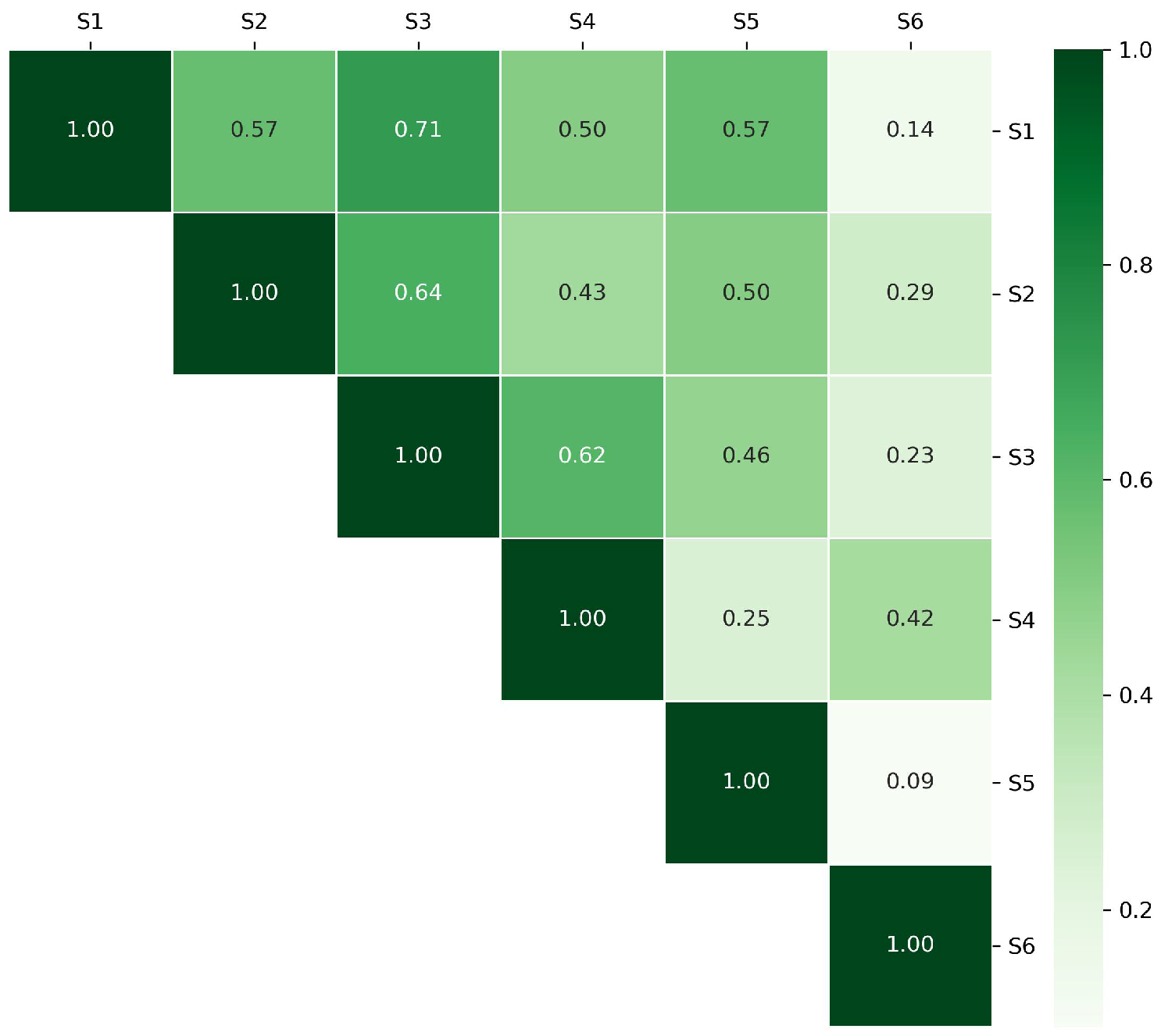
The heat map of the path similarity matrix is shown in Figure 2. Note that the path similarity matrix is symmetric with respect to the angle bisectors. To optimize storage efficiency, only the upper triangular portion of the matrix is retained.
The average similarity value of all paths is calculated to be U = 0.42 .
The following steps perform fuzzy clustering on six paths. Given the set S = { S 1 , S 2 , S 3 , S 4 , S 5 , S 6 } , the first path S 1 is selected as the center path for cluster T 1 . Paths S 2 , S 3 , S 4 , and S 5 are selected because their similarity with S 1 exceeds the threshold U = 0.42 , based on the similarity matrix Λ . These paths are then added to cluster T 1 , forming the first cluster as T 1 = { S 1 , S 2 , S 3 , S 4 , S 5 } .
Next, remove the paths S 1 , S 2 , S 3 , S 4 , S 5 from the set S, leaving the updated set S = { S 6 } .
Then, select S 6 from S as the center path for the next cluster T 2 . Repeat the above steps until S = . Finally, the two resulting path clusters are:
T 1 = { S 1 , S 2 , S 3 , S 4 , S 5 } T 2 = { S 6 , S 4 }
It can be observed that, through our fuzzy clustering, path S 4 simultaneously belongs to both clusters T 1 and T 2 . This approach helps increase the likelihood of finding test cases that cover path S 4 .

3.2. Constructing MF_CNNpro Model for Cluster Based on the Center Path

Generally, there are multiple paths within the same cluster. Constructing a separate surrogate model for each path would incur significant costs. Moreover, each model would only be applicable to a single path, which is inefficient. Thus, considering the high similarity among the paths within the same cluster, it is more practical and cost-effective to construct a single surrogate model for the entire cluster. This model can be based on the center path, which represents the common characteristics of all paths in the cluster.
This section introduces the surrogate model based on the Multi-Feature professional Convolutional Neural Network, MF_CNNpro (as shown in Figure 3), which is constructed using the center H 1 γ and serves the multiple paths within the same cluster. The MF_CNNpro model can reduce model training time and improve its utilization efficiency.
Algorithm 2 describes the construction and training of the MF_CNNpro model.
Algorithm 2 Establish and train MF_CNNpro Model
Input: Sample data X = { x 1 , x 2 , , x N } ; cluster center path H 1 γ ; training/test set partition ratio
Output: Trained MF_CNNpro model; model performance evaluation results on the test set
  1:
Initialize sample set V =
  2:
for each input x μ X  do
  3:
      Execute x μ to obtain the traversal path g ( x μ ) ; g ( x μ ) as auxiliary features
  4:
      Add the tuple ( x μ , auxiliary   features , y μ ) to the sample set V
  5:
      Compute the fitness f i t ( x μ ) using Equations (2) and (3)
  6:
     Find the first matching node position p o s f and the last matching node position p o s e between g ( x μ ) and H 1 γ ; Sate Normalize the positions using Equation (4):
  7:
      Construct the output feature y μ = f i t ( x μ ) , f i r s t ( x μ ) , e n d ( x μ )
  8:
end for
  9:
Split the sample set V into training set V t r a and test set V t e s t based on the given partition ratio
10:
Initialize the MF_CNNpro model with the following components:
   - Input layer: Matches the dimension of program input features (i.e., dimension of x μ )
   - Auxiliary input layer: Matches the dimension of the encoded traversal path (i.e., dimension of auxiliary features)
   - Output layer: 3-dimensional output (corresponding to f i t ( x μ ) , f i r s t ( x μ ) , e n d ( x μ ) )
11:
Train the MF_CNNpro model using the training set V t r a , with a multi-task loss function (to jointly optimize the three output features)
12:
Evaluate the trained model’s performance on the test set V t e s t (e.g., using MAE for regression tasks)
13:
Return the trained MF_CNNpro model and the corresponding test set evaluation results
(1)
The input feature vector and auxiliary feature
Let the input of the program be X = { x 1 , x 2 , , x N } , which represents the sample set, where N represents the number of inputs. Initialize sample set V = . In lines 2–3 of Algorithm 2, the program is executed on X, producing the set of covered mutant branches, which forms the traversal path
G ( X ) = { g ( x 1 ) , g ( x 2 ) , , g ( x N ) } .
The nodes included in the path referenced in this paper only record the mutant branches.
For our MF_CNNpro model, the input feature vector is the program input vector. Additionally, the traversal path set G ( X ) is used as an auxiliary feature when training the surrogate model, following the CNNpro model [13] (as shown in Figure 4) in line 4.
(2)
The three-dimensional out features
In the CNNpro model [13], only the fitness value (Equation (3)) is used as the output feature. Within a cluster, all paths share the same CNNpro model. However, if two different paths within the cluster have the same similarity to the center path, the CNNpro model is unable to distinguish which path the predicted data is better suited for. This limitation arises because, despite having the same similarity to the center path, these paths may contain distinct mutant branches.
In contrast, the output features of our MF_CNNpro model are three-dimensional, consisting of the fitness value and two position labels derived from a comparison with the center path. This enhancement allows the surrogate model to incorporate more comprehensive feature information from the paths within the same cluster, thereby improving its performance.
The model in Figure 4 includes one input feature, one auxiliary feature, and one output feature. In contrast, our model in Figure 3 [13] includes only one input feature, one auxiliary feature, and three output features.
Note that the surrogate model is constructed for multiple paths within the same cluster because we take the similarity of the paths into consideration. The model’s output features are three-dimensional, as we consider the differences between the paths within the same cluster.
The following describes the method for obtaining the fitness value and two position label output features derived from a comparison with the center path.
Let x u represent a sample input datum, and its traversal path is g ( x ) .
The fitness value f i t ( x μ ) is obtained based on the similarity between traversal path g ( x ) and center path H 1 γ According to Equations (2) and (3) in Line 5 of the algorithm.
In Line 6, p o s f ( x μ ) represents the position of the first node in traversal path g ( x μ ) that matches the center path H 1 γ , starting from index 0. Similarly, p o s e ( x μ ) refers to the position of the last node in g ( x μ ) that matches H 1 γ . These position values are normalized as follows:
f i r s t ( x μ ) = p o s f ( x μ ) | H 1 γ | 1 e n d ( x μ ) = p o s e ( x μ ) | H 1 γ | 1
where | H 1 γ | denotes the number of nodes in path H 1 γ .
In the MF_CNNpro, the output feature value corresponding to x μ is expressed as
y μ = ( f i t ( x μ ) , f i r s t ( x μ ) , e n d ( x μ ) )
Thus, for the input feature X, the corresponding output feature is
Y = ( F i t n e s s ( X ) , F i r s t ( X ) , E n d ( X ) )
The sample set is represented as
V = { ( X , Y ) } = { ( x 1 , y 1 ) , ( x 2 , y 2 ) , , ( x N , y N ) }
This sample set V is divided into a training set V t r a and a test set V t e s t , shown in Line 9.
Continuing with the example from the set of mutation-based paths S.
S 1 = M 5 , M 6 , M 7 , M 8 , M 12 , M 13 , M 15 , M 17 , M 19 , M 21 , M 23 , M 24 , M 25 , M 26
is the center path in cluster T 1 = { S 1 , S 2 , S 3 , S 4 , S 5 } .
Assuming x = ( 42 , 73 , 125 ) is an input in the sample set, its traversal path is
g ( x ) = M 5 , M 6 , M 7 , M 11 , M 13 , M 16 , M 18 , M 20 .
According to Equation (1), the fitness value is calculated as
f i t ( x ) = | S 1 g ( x ) | max ( | S 1 | , | g ( x ) | ) = 4 14 0.29 .
Using Equation (4), we compute
f i r s t ( x ) = p o s f ( x ) | S 1 | 1 = 0 14 1 = 0 e n d ( x ) = p o s e ( x ) | S 1 | 1 = 5 14 1 0.39 .
Thus, the output y = ( f i t ( x ) , f i r s t ( x ) , e n d ( x ) ) , i.e.,  y = ( 0.29 , 0 , 0.39 ) , corresponds to the sample input x = ( 42 , 73 , 125 ) in the MF_CNNpro model.
Following this method, a sample set V = { ( X , Y ) } is obtained.

3.3. Test Case Generation Using MF_CNNpro Model and PSO

Algorithm 2 describes test case generation using MF_CNNpro and PSO. The input of the algorithm is the clustering set T = { T 1 , T 2 , , T ħ } and the MF_CNNpro model. The output is the set of test case set generated for covering each path.

3.3.1. Selecting Excellent Initial Particles via MF_CNNpro Model

In lines 2 to 30, the main loop begins by checking if the cluster T r , r = 1 , 2 , , ħ is empty. If it is not, the algorithm proceeds.
In Line 3 of Algorithm 2, the MF_CNNpro model constructed from the center path is used to select the excellent particles corresponding to other paths within the cluster. This process is a key technique of the proposed method.
Note that the similarity among multiple paths within the same cluster is extremely high. To reduce the cost of constructing the surrogate model for each path within the cluster, each path can reuse the MF_CNNpro model, which is constructed based on the central path of the cluster. This model enables the other paths within the cluster to predict their own optimal initial particles.
The MF_CNNpro model, constructed using the center path, can be applied to all paths within the same cluster. While these paths are highly similar, each path has its own distinct characteristics. Therefore, the excellent particles predicted by the MF_CNNpro model for each path are expected to vary. To account for the diversity between a path and the center path, we introduce the concept of a similar objective function, which not only measures the similarity to the center path but also retains the unique characteristics of each individual path.
Let cluster T r = { H 1 γ , H 2 γ , , H | H | γ } contain | H γ | paths.
Define the similar objective function between path H i γ and center path H 1 γ based on MF_CNNpro model as
Y γ = ( F i t n e s s i γ ( X ) , F i r s t i γ ( X ) , E n d i γ ( X ) )
where F i t n e s s i γ ( X ) is the fitness function corresponding to their similarity.
The predicted value of input X, denoted as
Y ^ = ( F i t n e s s ( X ) , F i r s t ( X ) , E n d ( X ) )
is obtained from the MF_CNNpro model of the center path H 1 γ .
The absolute error between the predicted output and the similar objective vector is then used to determine whether a particle is considered excellent for a given path within the cluster.
Let the absolute error between the predicted value Y ^ and the similar objective value Y γ be denoted as E ( X ) :
E ( X ) = Y ^ Y γ = F i t n e s s ( X ) F i t n e s s i γ ( X ) + F i r s t ( X ) F i r s t i γ ( X ) + E n d ( X ) E n d i γ ( X )
Using the absolute error, we can evaluate whether the input X corresponds to an excellent particle of H 1 γ .
Example: Continuing with the set of mutation-based paths S, S 1 = M 5 , M 6 , M 7 , M 8 , M 12 , M 13 , M 15 , M 17 , M 19 , M 21 , M 23 , M 24 , M 25 , M 26 is the central path of cluster T 1 = { S 1 , S 2 , S 3 , S 4 , S 5 } . We then describe how the optimal particle swarm for path S 1 is selected using the MF_CNNpro model, which serves as the initial population for the PSO algorithm to generate the test case covering S 1 .
From Equation (4), the fitness corresponding to the similarity of S 1 in T 1 with itself is calculated as
F i t n e s s 1 1 ( X ) = 1
Using Equations (5) and (6), the following values can be calculated for S 1 with respect to itself:
F i r s t 1 1 ( X ) = 0 14 1 = 0 E n d 1 1 ( X ) = 13 14 1 = 1
Therefore, the similarity objective function between the center path S 1 and itself, as output by the MF_CNNpro model, is
Y 1 = ( F i t n e s s 1 ( X ) , F i r s t 1 ( X ) , E n d 1 ( X ) ) = ( 1 , 0 , 1 )
For S 1 , suppose its sample input test case set is X = { x 1 , x 2 , x 3 , x 4 , x 5 } , where
x 1 = ( 5 , 5 , 5 ) , x 2 = ( 65 , 15 , 35 ) , x 3 = ( 20 , 35 , 46 ) , x 4 = ( 15 , 23 , 34 ) , x 5 = ( 11 , 22 , 35 )
The output values predicted by MF_CNNpro model are as follows:
Y ^ 1 = ( 0.81 , 0.05 , 0.99 ) , Y ^ 2 = ( 0.08 , 0.1 , 0.22 ) , Y ^ 3 = ( 0.54 , 0 , 0.98 ) , Y ^ 4 = ( 0.46 , 0 , 0.93 ) , Y ^ 5 = ( 0.15 , 0 , 0.33 )
Next, the absolute error is calculated using Equation (7), using x 1 as an example:
E ( x 1 ) = | Y ^ 1 Y 1 | = 0.81 1 + 0.05 0 + 0.99 1 = 0.25
Using the same method,
E ( x 2 ) = 1.8 , E ( x 3 ) = 0.48 , E ( x 4 ) = 0.61 , E ( x 5 ) = 1.5
Assume that two excellent particles are needed. Among five particles, x 1 and x 3 are selected as the initial population of PSO because their absolute error values ( E ( x 3 ) = 0.26 and E ( x 3 ) = 0.5 ) are the smallest. Therefore, x 1 = ( 5 , 5 , 5 ) and x 3 = ( 20 , 35 , 46 ) with the smallest errors are used as the initial population of PSO corresponding to S 1 .
Based on the above method, MF_CNNpro model of S 1 can predict the excellent particles for the other paths in cluster T 1 .
Paths S 2 and S 5 exhibit the same similarity to center path S 1 , both with a similarity score of 0.57. Therefore, by considering S 2 and S 5 as examples, we demonstrate that, despite their identical similarity to the center path, our method is still capable of selecting diverse, high-quality particles for each of them.
For the path S 2 = M 1 , M 4 , M 6 , M 7 , M 8 , M 10 , M 14 , M 15 , M 18 , M 20 , M 21 , M 23 , M 25 , M 26 , the fitness corresponding to the similarity between S 2 and S 1 can be calculated using Equation (1) as
F i t n e s s 2 1 ( X ) = | S 1 S 2 | max | S 1 | , | S 2 | = 8 14 0.57
Using Equations (5) and (6),
F i r s t 2 1 ( X ) = p o s f X | S 1 | 1 = 1 14 1 0.08 E n d 2 1 ( X ) = p o s e ( X ) | S 1 | 1 = 13 14 1 = 1
Thus, the similarity objective output between paths S 2 and S 1 is
Y 2 = ( 0.57 , 0.08 , 1 )
For the input x 6 = ( 3 , 5 , 4 ) , using MF_CNNpro model of S 1 , the predicted value is
Y ^ 6 = ( 0.71 , 0.02 , 0.94 )
The absolute error value is
E ( x 6 ) = | Y ^ 6 Y 2 | = | 0.71 0.57 | + | 0.02 0.08 | + | 0.94 1 | = 0.26
Using MF_CNNpro model of S 1 , the absolute error values corresponding to path S 2 are shown in Table 1.
In Table 1, since E ( x 6 ) = 0.26 and E ( x 10 ) = 0.11 are the smallest values in the absolute error, x 6 = ( 3 , 5 , 4 ) and x 10 = ( 36 , 71 , 80 ) are selected as the excellent particles for path S 2 .
Similarly, the similarity objective output between paths S 5 and S 1 is Y 5 = ( 0.57 , 0 , 0.69 ) .
Using MF_CNNpro model of S 1 , the absolute error values corresponding to path S 5 are obtained and shown in Table 2:
In Table 2, since E ( x 10 ) = 0.32 and E ( x 12 ) = 0.35 are the smallest absolute errors, the particles x 10 and x 12 are selected as the excellent particles for path S 5 .
Note that from Table 1 and Table 2, we can see that x 6 and x 10 are the same inputs of the MF_CNNpro model for paths S 2 and S 5 . However, despite the similarity between S 2 and S 5 with S 1 being the same, the different node compositions in S 2 and S 5 lead to distinct absolute errors when predicted by MF_CNNpro model of S 1 . The MF_CNNpro models in previous literature were unable to distinguish the optimal particles between S 2 and S 5 . Specifically, using our model, x 10 can be selected as a particle for both S 2 and S 5 , while x 6 can only be selected as a particle for S 2 , but not for S 5 . This study demonstrates that the MF_CNNpro model we constructed considers both particle differences and path diversity during training and prediction.

3.3.2. Test Case Generation for Paths Using PSO

Algorithm 3 is designed to generate test cases for each cluster using the MF_CNNpro model in conjunction with the Particle Swarm Optimization (PSO) algorithm. The core process can be divided into three stages: initialization, iterative search, and result collection. The specific steps and key points are as follows:
Initialization Stage:
The particle swarm and algorithm parameters are initialized. An empty particle swarm X ¯ = { x ¯ 1 , x ¯ 2 , , x ¯ w } is created, and the core PSO parameters (such as inertia weight linearly decreasing from 0.9 to 0.4, acceleration coefficients c 1 = c 2 = 1.5 , and particle count w = 30 ) are configured. The cluster index i is initialized to 1, indicating the first cluster to be processed. The outer loop is then activated, with the condition that the current cluster T i is non-empty to initiate.
Initial Particle Swarm Generation: A batch of initial test cases is randomly generated as the candidate set for the particle swarm. The MF_CNNpro model, based on the central path H 1 γ , is used to predict the fitness of the candidate test cases (the higher the fitness, the greater the potential for the test case to cover the target path).
Subsequently, the initial particle swarm is constructed by selecting the top w test cases from the candidate set with the highest fitness. This forms the initial particle swarm X ¯ for the current path H i γ .
PSO Iterative Optimization: The iterative parameters are initialized by setting the iteration counter θ = 0 with maximum iterations g = 10,000. Simultaneously, the velocity, personal best (pbest, which records the individual particle’s historical optimal position), and global best (gbest, which records the global optimal position of the entire particle swarm) are initialized for each particle in the swarm.
The inner loop is then activated, with the dual conditions of “no test case covering H i γ has been found” and “iteration count θ has not reached the maximum value g” to perform the PSO optimization process. The loop terminates when either of these conditions is satisfied. Next, the fitness of each particle (test case) in the current particle swarm is calculated using the MF_CNNpro model, which is then used to update the optimal solutions and generate a new particle swarm X ¯ . Subsequently, the iteration count is updated by incrementing the counter θ after each evolution.
Algorithm 3 Test Case Generation using MF_CNNpro and PSO
Input: Cluster set T = { T 1 , T 2 , , T ħ } ; MF_CNNpro model; maximum number of iterations g for particle swarm update.
Output: Generated test case set for each cluster.
  1:
Initialize particle swarm X ¯ = { x ¯ 1 , x ¯ 2 , , x ¯ w } = , PSO parameters (inertia weight, acceleration coefficients, etc.); set i = 1 .
  2:
while  T i  do
  3:
      Randomly generate candidate test cases; predict their fitness values using the MF_CNNpro model of the center path H 1 γ .
  4:
      Select top-w candidate test cases with highest fitness as the initial particle swarm X ¯ = { x ¯ 1 , x ¯ 2 , , x ¯ w } for path H i γ .
  5:
      Set iteration counter θ = 0 ; initialize particle velocities, personal best ( p b e s t ), and global best ( g b e s t ) of X ¯ .
  6:
      while No test case covering H i γ is found and  θ < g  do
  7:
         Predict fitness of each particle in X ¯ using MF_CNNpro.
  8:
         Update p b e s t for each particle (if current fitness >  p b e s t fitness).
  9:
         Update g b e s t of the swarm (if best p b e s t fitness >  g b e s t fitness).
10:
         Perform PSO evolution operations: update particle velocities and positions (using standard PSO velocity update formula).
11:
         Generate new particle swarm X ¯ from updated positions.
12:
          θ = θ + 1
13:
      end while
14:
      if  θ g  then
15:
         Record the test case corresponding to g b e s t as the covering test case for H i γ .
16:
      else
17:
         Record “No covering test case found for H i γ ”.
18:
      end if
19:
       i = i + 1
20:
end while
21:
Return the collected test case set for all non-empty clusters.
Result Recording and Cluster Iteration: The results for the current path are recorded.
If the inner loop terminates due to “a test case covering H i γ being found” ( θ g ), the test case corresponding to the global best (gbest) is recorded as the valid covering test case for H i γ . If the loop terminates due to “the iteration count exceeding the maximum limit” ( θ > g ), it is marked as “no covering test case for H i γ found.”
The cluster processing then proceeds by incrementing the cluster index i, and the outer loop continues to process the next cluster until all non-empty clusters have been processed.
Finally, the results are output: the test case set for all clusters is returned, including both valid test cases and those marked as “no test case found.”
In PSO, the Hypercube Boundary is a boundary constraint approach for high-dimensional optimization problems (extending a three-dimensional cube to D dimensions, where D is the dimension of the optimization problem). The improved version of PSO is referred to as PSOpro.
By defining independent upper and lower bounds [ x min , d , x max , d ] for each dimension ( d = 1 , 2 , , D ), and combining these with targeted boundary handling strategies and improvements to the standard PSO equations, PSOpro addresses the issue of local optima in high-dimensional spaces. The key advantage is the ability to break the “attraction trap” associated with local optima in three-dimensional spaces by constraining the search space, guiding particle exploration, and balancing global and local search. The core logic of PSOpro is to prevent particle divergence through rigid constraints in high-dimensional spaces, while employing boundary interaction mechanisms to compel particles to escape from local optimal regions.
To construct a hypercube coordinate system, the program input is set as X = ( x 1 , x 2 , , x d ) , where d represents the dimension of the variables, and x i [ a i , b i ] (with a i and b i being the minimum and maximum values of the boundary for variable x i ).
According to the input dimension d, the search space is divided into d-dimensional hypercubes, resulting in 2 d vertices. Each hypercube can be seen as a region containing several particles.
The hypercube boundary value method is used to update w particles. For each dimensional variable x i [ a i , b i ] , two types of boundary particles are selected: one at the minimum boundary a i and one at the maximum boundary b i . These particles form the vertices of the d-dimensional hypercube: ( a 1 , a 2 , , a d ) , ( b 1 , a 2 , , a d ) , , ( b 1 , b 2 , , b d ) . Then, w particles are randomly selected from these 2 d vertex particles to supplement the particle swarm.

4. Example Analysis

4.1. Research Questions

This section describes three verification problems, which are based on the three main parts of our method.
  • RQ1: Does fuzzy clustering help bolstering the effectiveness of mutation testing?
    It is not surprising that one path may resemble paths from different clusters. Consequently, it is natural to consider fuzzy clustering when dividing the path set into distinct groups. In this study, we investigate whether and to what extent the overlap among different clusters, an expected outcome of fuzzy clustering, impacts the effectiveness of mutation testing.
  • RQ2: What is the performance of the improved models (CNNpro)?
    To solve the problem that evolutionary algorithms face in achieving path coverage, predictive models are built. Then, to test if the basic CNN we chose is reasonable and works well, we compare it with four other basic prediction models. Also, to check how well our improved model (CNNpro) performs, we use four different measures. These measures help us look at different parts, like accuracy, ability to generalize, use of resources, and how fast it runs.
  • RQ3:How does the CNNpro_PSO method improve the speed of creating test data?
    The improved model and the PSO method are joined together (CNNpro_PSO). This combination aims to speed up test data generation. To test its performance, we use three other methods and four metrics for comparison: success rate, iteration count, time spent, and mutation score. Finally, we run hypothesis tests on the results to show our method’s importance.

4.2. Experiment Settings

The experiment was conducted on a desktop computer equipped with an Intel Core i5-13600KF processor and 32 GB of RAM, using the Python programming language (Python 3.11.3).
Table 3 above presents basic information about the six subject programs. These programs exhibit significant differences in terms of code size, data structures, and functional scope. P1 to P3 are benchmark programs widely used in software testing research [32,33,34]. P4 is a system designed to analyze energy consumption across industrial facilities. P5 is a real-time system resource monitoring module for comprehensively tracking various performance metrics of computer systems. P6 is a complete supply chain management solution that covers the entire material flow process from suppliers to customers.
Testing on diverse software domains demonstrates the strong applicability of the proposed method, confirming its effectiveness for various practical applications.

4.2.1. Procedure for RQ1

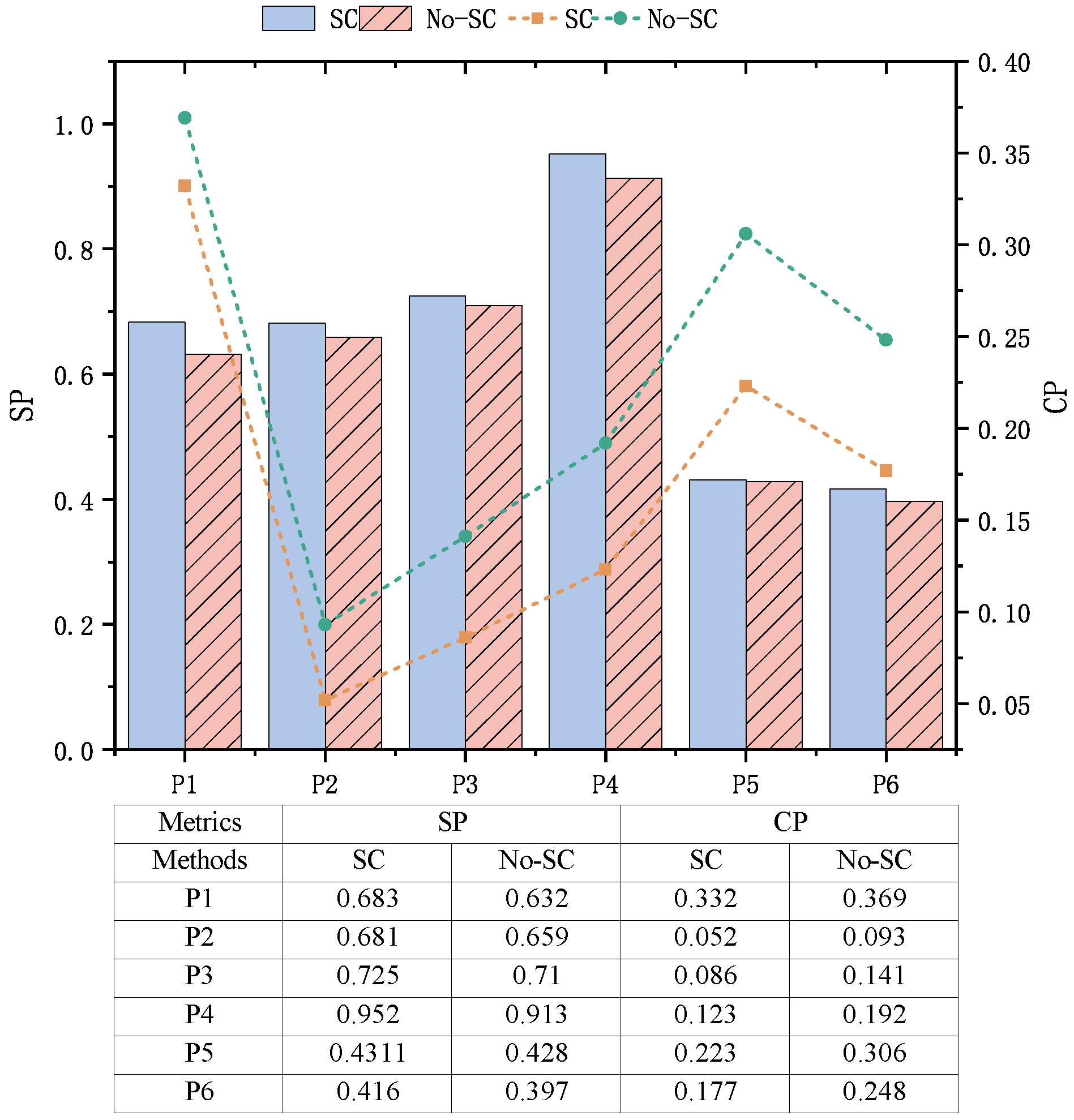
In this experiment, two methods (SC, No-SC) are compared, and their performance is evaluated using two metrics: cluster separation (SP) and cluster compactness (CP) [35].
SC: This method first sorts the paths in descending order of coverage difficulty and then selects the most difficult-to-cover paths as the cluster centers. This makes it easier to obtain a higher SP value (better inter-cluster separation) and a lower CP value (better intra-cluster compactness) in calculations.
No-SC: This method randomly selects paths as cluster centers. This often results in a lower SP value and a higher CP value in calculations.
SeParation degree (SP) metric is used to measure the separation degree between different clusters. It is calculated as the ratio of the average inter-cluster distance to the average distance of all samples (pathes).
S P = d inter ¯ d all ¯
d inter ¯ (Average Inter-cluster Distance): First, calculate the distance between the centers of every two different clusters, then take the arithmetic mean of all inter-cluster center distances. Cluster center paths: H 1 1 , H 1 2 , , H 1 ħ .
d inter ¯ = 2 ħ ( ħ 1 ) γ = 1 ħ 1 j = γ + 1 ħ distance ( H 1 γ , H 1 j )
distance ( H 1 γ , H 1 j ) = 1 ( H 1 γ , H 1 j ) is computed based on the similarity between center paths H 1 γ and H 1 j .
d all ¯ (Average Distance of All Paths): The arithmetic mean of distances between any two different samples in the dataset. For a path set with n samples, ( S i , S j ) represent any two distinct samples).
d all ¯ = 2 n ( n 1 ) i = 1 n 1 j = i + 1 n 1 ( S i , S j )
A larger SP value indicates more significant separation between clusters, corresponding to better clustering discrimination.
ComPactness degree (CP) metric is used to measure the aggregation degree of samples within a single cluster, and it is calculated as the ratio of the mean of average intra-cluster distances to the average distance of all samples to the global center.
C P = 1 ħ i = 1 ħ d intra , i ¯ d center ¯
d intra , i ¯ (Average Intra-cluster Distance of the i-th Cluster): The arithmetic mean of distances from all samples in the i-th cluster to its center T i . For the i-th cluster with n i samples.
d intra , γ ¯ = 1 T γ s j cluster i distance ( S j , H 1 γ )
distance ( S j , H 1 γ ) = 1 ( S j , H 1 γ ) is computed based on the similarity between the center paths S j and H 1 γ .
d center ¯ is the average distance of all samples to the global center.
A smaller CP value indicates that samples within the cluster are more densely distributed around the cluster center, corresponding to better clustering compactness.
The Clustering Rate (CR) is calculated by dividing the number of clusters by the total number of paths.
CR = Number   of   Clusters Total   Number   of   Paths
The key evaluation criterion is that a smaller CR value is better. This metric directly reflects the effectiveness of path redundancy reduction. A lower CR value indicates that a higher efficiency of similar path merging has been achieved with fewer clusters, leading to more effective elimination of redundant paths.

4.2.2. Procedure for RQ2

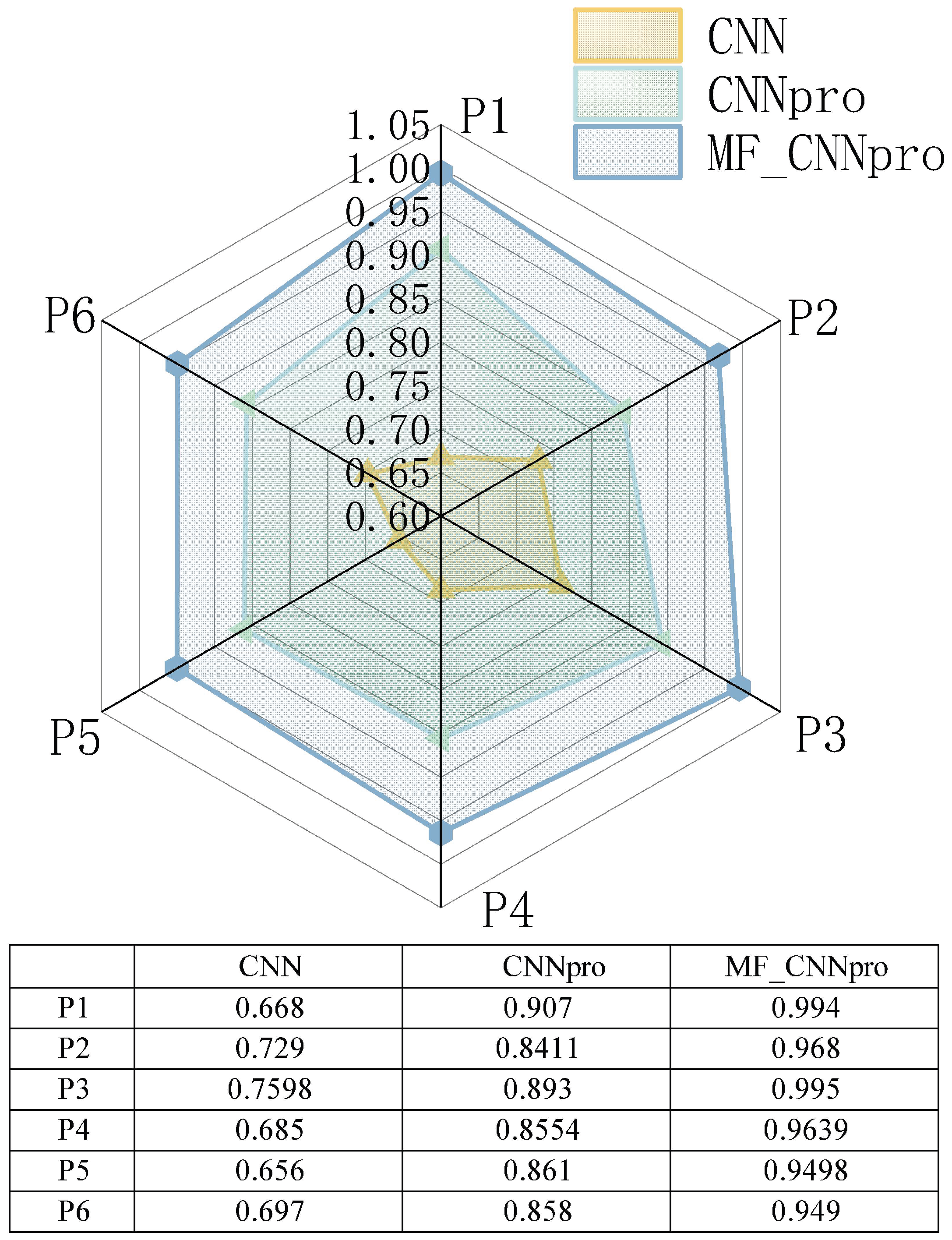
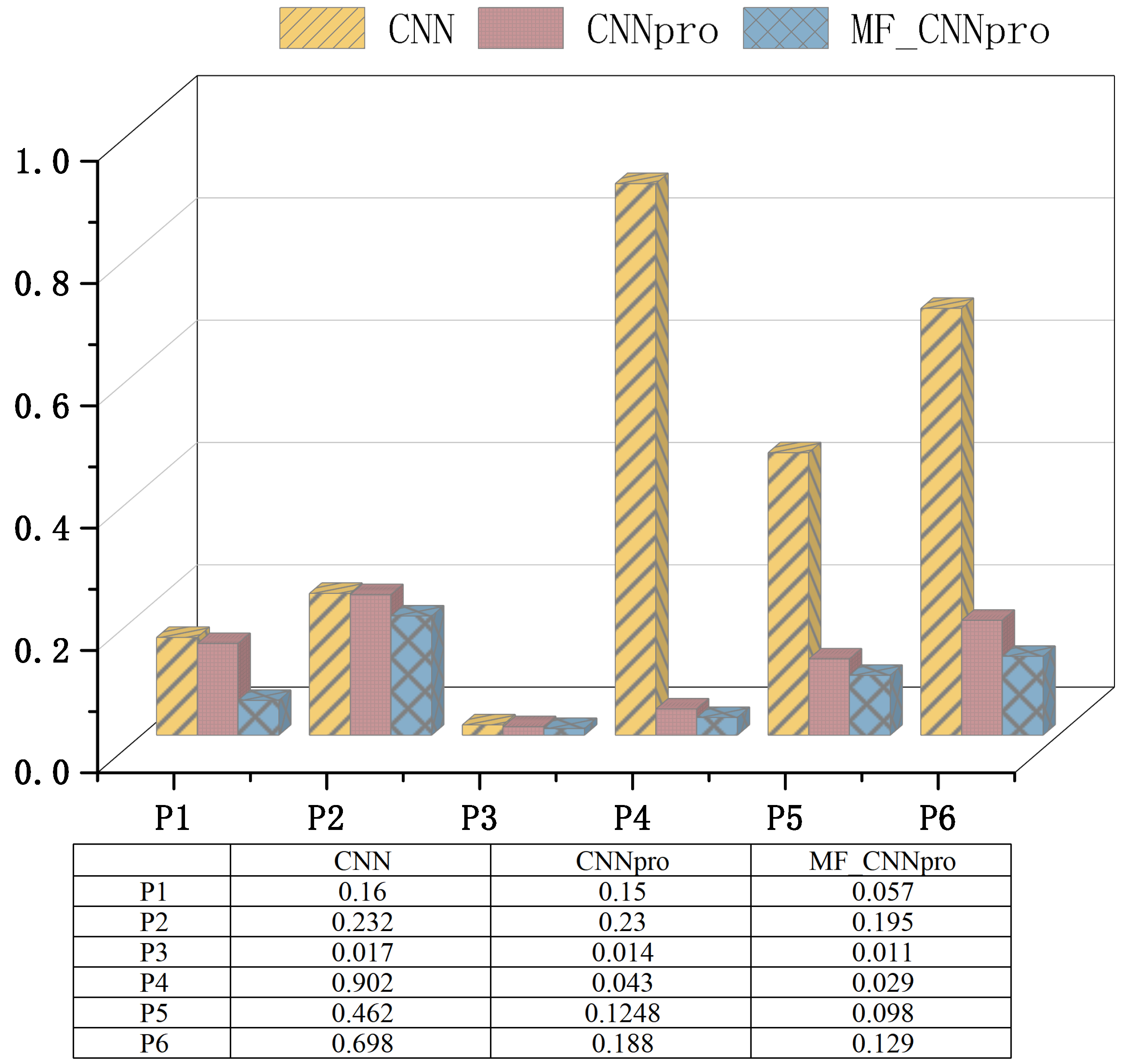
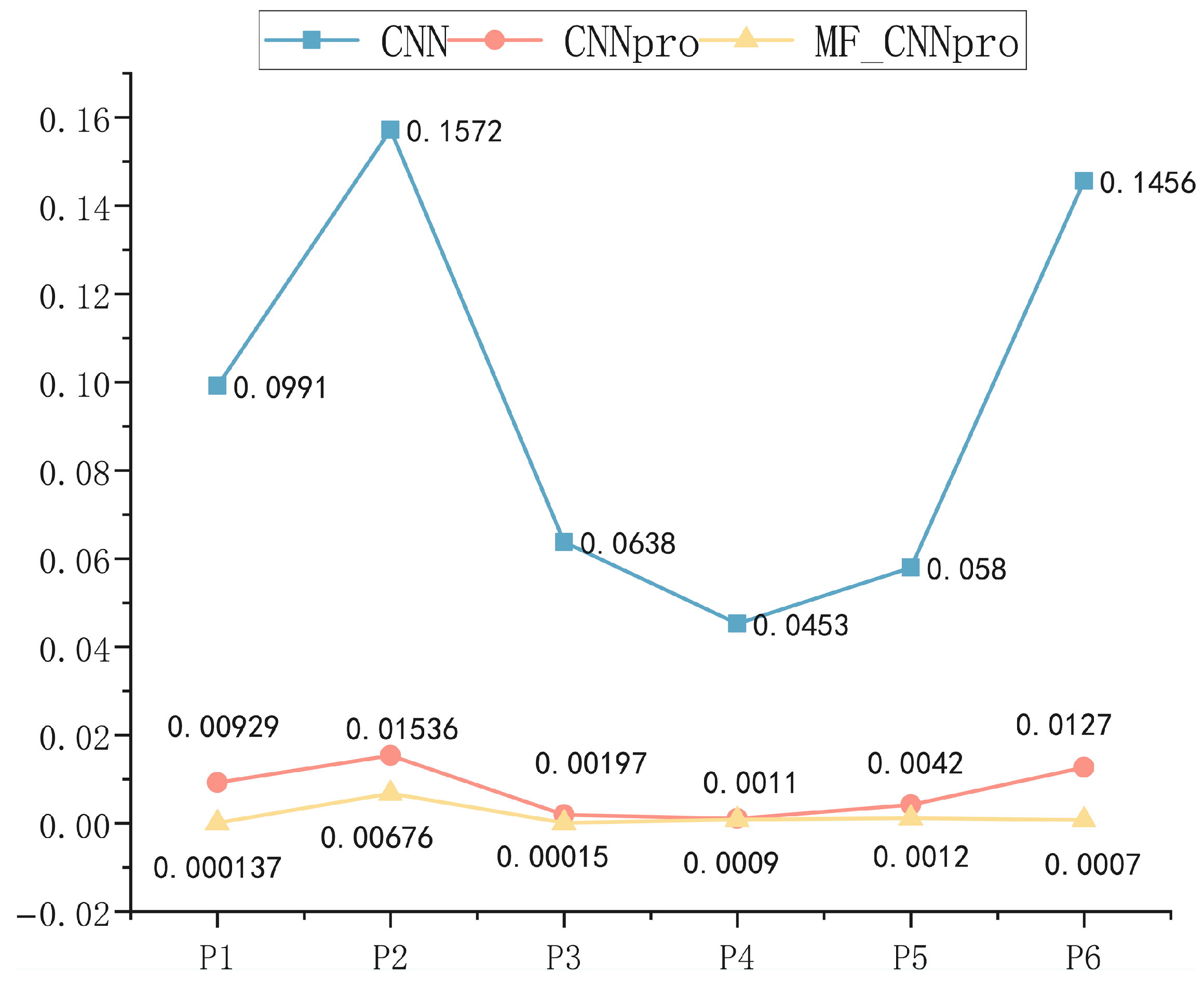
In this experiment, six prediction models (traditional CNN [4], CNNpro [13], and PSO [5]) are selected for comparison. Four metrics [13] are used to verify the effectiveness of the MF_CNNpro model.
These metrics encompass key model characteristics, including accuracy, generalization ability, resource usage, and computational efficiency.
  • Index Agreement ( I A ): It is used to measure the consistency between the predicted values and the true values.
  • U-statistic: This metric tests for model bias by focus on measuring error in prediction between the predicted and true values, which helps find systematic errors and ensures the model is fair. A U-statistic closer to 0 indicates higher accuracy.
  • Mean Squared Error ( M S E ): It evaluates the average magnitude of errors in the model’s predictions by calculating the squared differences between predicted and actual values.
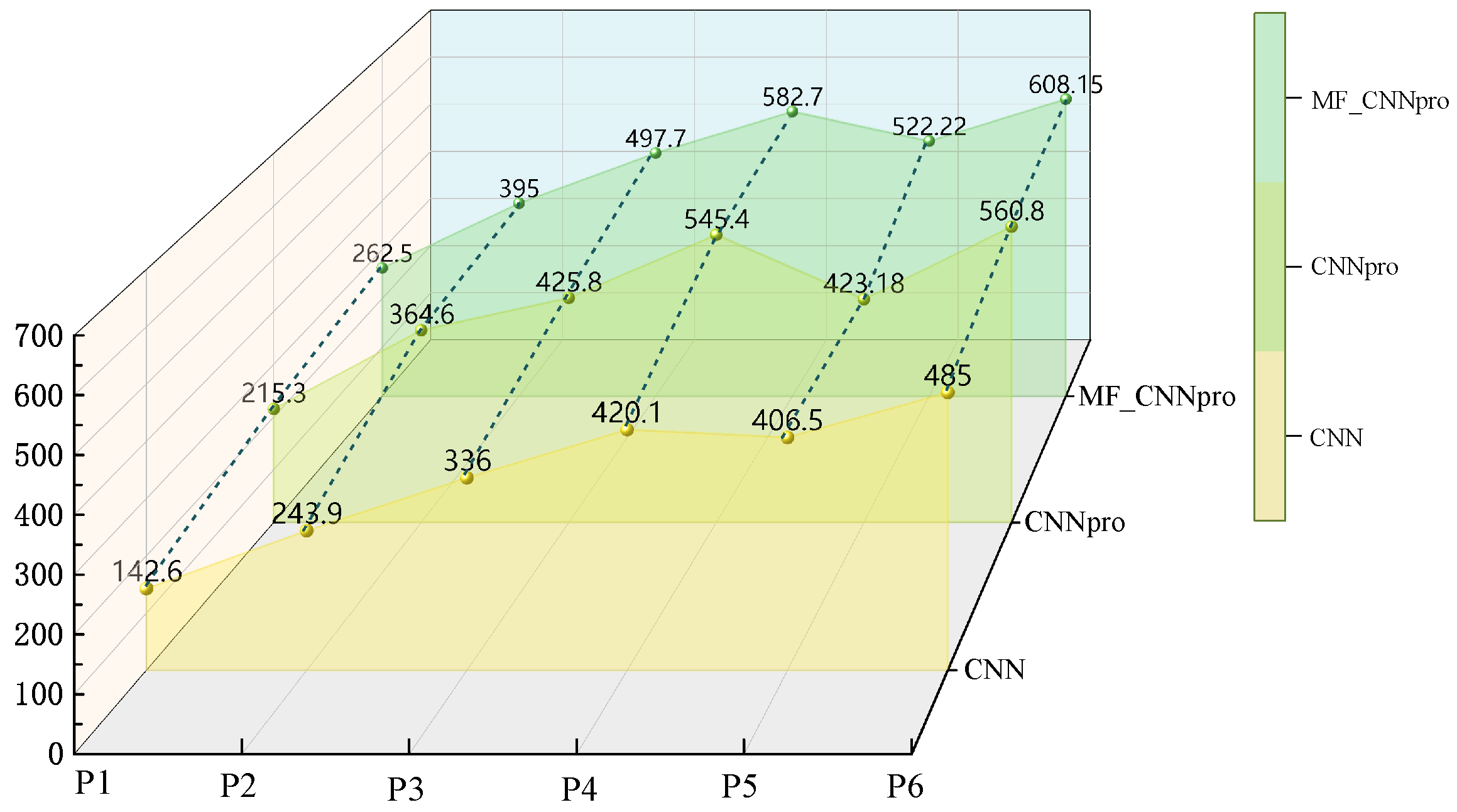
  • The Memory Consumption ( M i B ): It measures the memory used by the prediction model when it runs. Memory use is important because it shows how complex the model is and how much computing power it needs. A lower MiB value means the model uses less memory, so it is more lightweight and efficient. This is very important when working with large datasets.
During the construction of the predictive model, several factors are considered in the dataset configuration, including sensitivity adjustment, feature selection, outcome metrics, sample distribution rationality, and scientific data partitioning.
Regarding sensitivity adaptation, redundant information irrelevant to the prediction target is removed, leaving core input features that represent the program’s input traversal paths and output values (adaptation values/path start and end positions). Additionally, heterogeneous traversal path samples triggered by different inputs, as well as fluctuation samples of adaptation values triggered by the same input across multiple paths, are included to strengthen the coverage of the inherent “input-path-outcome” relationships.
Next, a multi-objective outcome metric system is constructed, with the program’s adaptation value as the primary target and the start and end positions of the traversal path as secondary metrics. This framework combines primary and secondary objectives to achieve precise prediction of key nodes within the path.
Furthermore, the sample size is set at 3000, balancing training costs and prediction accuracy. This sample size avoids the resource consumption and long training cycles associated with datasets exceeding ten thousand samples, while also addressing overfitting and insufficient generalization in datasets smaller than a thousand samples. The sample distribution is optimized to ensure that program input features are uniformly distributed within the valid value range, covering boundary intervals, middle intervals, and critical threshold intervals. The adaptation values are uniformly distributed within the 0–1 range, and the path position samples cover start and end nodes for various path types. This ensures that the model can learn input-output relationships in a balanced manner.
Finally, a scientific data partitioning strategy is applied. Stratified sampling is used to divide the 3000 samples into training and testing sets with a 70:30 ratio. Stratification is based on adaptation value intervals (0–0.2, 0.2–0.4, 0.4–0.6, 0.6–0.8, 0.8–1.0), ensuring coverage of all variance branches (defects). This ensures that the sample distribution in each dataset aligns with the overall dataset, avoiding distribution biases caused by random sampling.

4.2.3. Procedure for RQ3

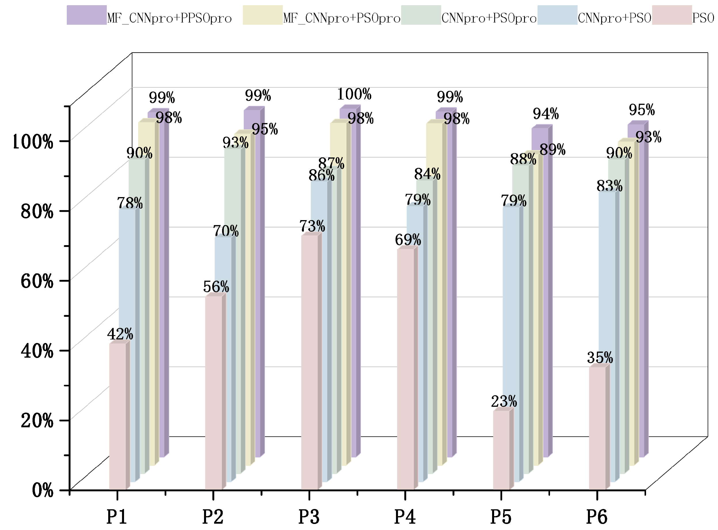
Algorithm 3 utilizes the MF_CNNpro model integrated with the Particle Swarm Optimization (PSO) algorithm (denoted as MF_CNNpro+PSO) to generate test cases for each cluster. Given the presence of multiple clusters, parallel computing is employed to implement Algorithm 3 (denoted as MF_CNNpro+PPSO), aiming to enhance computational efficiency.
The CNNpro and the proposed MF_CNNpro models, compared to the traditional CNN model, have not introduced many changes in terms of network structure, convolution kernel size, padding method, stride, or pooling operations. These model parameters are determined through repeated experimentation to obtain empirical values. Specifically, the model uses three convolutional layers to progressively extract features, with all convolutional layers using a kernel size of 2 and ’same’ padding to maximize information preservation under the limited 3D input features. A default stride of 1 is used to ensure high-resolution feature extraction. Given the relatively small input dimensions, the paper deliberately avoids pooling operations to prevent information loss, instead employing a combination of strategies such as BatchNormalization, Dropout, and L2 regularization to control overfitting.
To validate the performance of the proposed method, three benchmark approaches are selected for comparison: the traditional PSO algorithm, CNNpro combined with PSO (denoted as CNNpro+PSO), and CNNpro combined with parallel PSO (denoted as CNNpro+PSOpro).
Three key evaluation metrics are employed for a comprehensive performance assessment: success rate (to measure the effectiveness of test case generation), number of iterations (to assess convergence efficiency), and time consumption (to evaluate computational efficiency) [5,11,12,13].
The success rate is defined as the ratio of the number of successful test data detections to the total number of algorithm executions. A higher success rate indicates better performance of the corresponding algorithm.
The time used and the number of iterations for each successful search show how efficient the algorithm is. In general, less time and fewer iterations mean the search is more efficient.

4.3. Experimental Process

4.3.1. Answer to RQ1

As shown in Figure 5, this experiment investigates the clustering performance of six measurement programs ( P 1 to P 6 ) using both SC and No-SC methods. Two metrics are employed: clustering separation (SP, where a higher value indicates better performance) and clustering compactness (CP, where a lower value indicates better performance).
Analysis of the cluster separation (SP) metric shows that, among the six measured program paths, SC outperforms No-SC in five of the six samples: P 1 , P 2 , P 4 , P 5 , and P 6 . The advantage is most significant in the P 4 sample, where the SP value of SC is 0.039 higher than that of No-SC. The smallest advantage is observed in the P 5 sample, with a difference of only 0.003. The only exception is the P 3 sample, where No-SC’s SP value (0.725) is slightly higher than SC’s (0.710), with a small difference of 0.015. However, this difference is minimal and does not affect the overall performance of SC.
Regarding the cluster compactness (CP) metric, the CP value of SC is consistently lower than that of No-SC across all six samples, fully aligning with the evaluation criterion that “smaller CP values indicate better performance.” The largest difference is observed in the P 2 sample, where the CP value of SC is reduced by 0.041 compared to No-SC. The smallest difference occurs in the P 1 sample, where the reduction is 0.037, still maintaining a stable advantage for SC.
In conclusion, the SC method (the proposed method) outperforms the No-SC method overall. SC improves cluster separation in the majority of samples and reduces cluster compactness in all samples, thereby better achieving the ideal clustering goal of large between-cluster differences and small within-cluster differences.
In terms of the Clustering Rate (CR) in Table 4, among all the tested programs, the SC method consistently outperforms the NO-SC method, with a significant average difference between their clustering rates. Specifically, the average clustering rate of the SC method is calculated as
22.00 + 55.56 + 50.00 + 19.41 + 16.78 + 15.38 6 % 29.86 % ,
while the average clustering rate of the NO-SC method is 34.52%.
This shows that the SC method’s average clustering rate is approximately 4.66 percentage points lower than that of the NO-SC method, demonstrating the SC method’s significant advantage in merging similar paths and reducing the number of redundant clusters. As a result, the SC method exhibits a higher overall efficiency in path redundancy reduction.
The most notable difference is observed in program P5, where the SC method achieves a clustering rate of 16.78%, while the NO-SC method achieves 27.78%, resulting in a gap of 11 percentage points. This indicates that in scenarios with higher path similarity, the SC method is more effective at identifying and merging similar paths. It effectively avoids the redundant clustering caused by the random center selection in the NO-SC method.
The superior clustering performance of the SC method can be attributed to the collaborative design logic it employs. Unlike the NO-SC method, which randomly selects centers, the SC method chooses the most difficult-to-cover paths as cluster centers. This approach fundamentally avoids the potential issues of center overlap or insufficient center representativeness that may arise in the NO-SC method.
This revised approach ensures that the SC method is more efficient in identifying and merging similar paths, thus providing a more refined clustering process with better path redundancy reduction.

4.3.2. Answer to RQ2

Figure 6 shows the Index of Agreement (IA) values for CNN, CNNpro, and the proposed MF_CNNpro models across six program paths. Higher IA values indicate better consistency between predicted and true values, with an IA value closer to 1 representing superior accuracy.
The CNN model performs the worst, with an average IA of 0.6991 and no path exceeding 0.76, indicating weak consistency and low accuracy. Its standard deviation is 0.034, showing moderate fluctuation across paths. CNNpro significantly improves with an average IA of 0.8693, falling into the “good” category. It has the smallest standard deviation (0.025), indicating strong adaptability and stability. The MF_CNNpro model outperforms the others with an average IA of 0.9668, close to the ideal value of 1, and a minimal standard deviation of 0.018, showing excellent consistency and stability across paths. In conclusion, MF_CNNpro offers the best accuracy and stability in predicting program paths.
Figure 7 presents the U-Statistic values of the CNN, CNNpro, and MF_CNNpro models across six program paths. A U-Statistic closer to 0 indicates lower model bias and higher prediction accuracy.
With respect to the overall control of bias, the CNN model performs the worst, with a mean U-Statistic of 0.4118, indicating substantial global systematic error. Its standard deviation reaches 0.346, the largest among the three models, reflecting pronounced bias fluctuations across different program paths and highly unreliable global bias control. The CNNpro model achieves a moderately superior performance, with a mean U-Statistic reduced to 0.1248 (approximately 30% of that of CNN), demonstrating a significant reduction in overall error, accompanied by a relatively low standard deviation of 0.077.
The MF_CNNpro model exhibits the best overall performance due to multi-feature optimization, achieving the lowest mean U-Statistic of 0.0865 among the three models, indicating minimal systematic error. Its standard deviation is 0.066, showing limited fluctuation. This demonstrates that MF_CNNpro outperforms both CNN and CNNpro in terms of overall bias control and stability across program paths.
In conclusion, from a practical application standpoint, MF_CNNpro is the optimal choice, as it not only achieves the lowest overall bias but also maintains reliable performance paths such as P4.
Figure 8 shows the MSE values of CNN, CNNpro, and the proposed MF_CNNpro model across six program paths. Lower MSE values indicate better prediction accuracy.
The error control capabilities of the models are clearly ranked: CNN has the highest error, with a mean MSE of 0.0915 and path values ranging from 0.0453 to 0.1572. Paths P2 and P6 have the largest errors, failing to meet high-precision requirements. CNNpro reduces the error significantly, with a mean MSE of 0.0074 (a 91.9% reduction compared to CNN) and values ranging from 0.0011 to 0.01536, indicating stable low errors. The MF_CNNpro model shows the best performance, with a mean MSE of 0.0015 (a 79.7% reduction compared to CNNpro and 98.3% compared to CNN). Except for P2 (0.00676), all other paths have values below 0.0013, showing near-zero error.
In the high-difficulty P2 path, all models show higher errors, but MF_CNNpro (0.00676) still performs better than CNNpro (0.01536) and CNN (0.1572). In P5, both MF_CNNpro (0.0012) and CNNpro (0.0042) perform well, while CNN (0.058) shows a higher error.
In conclusion, MF_CNNpro is the optimal choice due to its near-zero error and strong adaptability across different paths.
Figure 9 presents the MiB values of CNN, CNNpro, and the proposed MF_CNNpro model across six program paths. MiB is commonly used to measure the model’s storage or resource consumption, with higher values indicating greater demand for storage or hardware resources.
In terms of overall resource usage, the three models exhibit a clear increasing trend: CNN has the lowest resource demand, with a mean MiB value of approximately 339.0, and path values ranging from 142.6 to 485. Path P6 (485) exhibits the highest resource consumption, while P1 (142.6) consumes the least. CNNpro shows a significant increase in resource demand compared to CNN, with a mean MiB of 452.5, representing a 33.5% increase. Path values range from 215.3 to 560.8, with P6 (560.8) having the highest usage. MF_CNNpro exhibits the highest resource consumption, with a mean MiB of 496.4, representing a 9.7% increase over CNNpro and a 46.4% increase over CNN. The path values range from 262.5 to 608.15, with P6 (608.15) having the highest usage, and P1 (262.5) having the lowest.
From the training curves in Figure 10, both the training loss, MAE, and MSE decreased steadily as the number of epochs increased, while the corresponding metrics on the validation set also showed a decline in the early stages, indicating good model convergence. Meanwhile, the learning rate continued to decay according to the scheduled plan, ensuring stable optimization in the later stages.
In comparison to traditional CNN models, both the CNNpro and the proposed MF_CNNpro models maintain consistent configurations in terms of network structure, kernel size, padding method, stride, and pooling operations. The parameters of these models were determined through iterative experimentation, leading to empirical values. Specifically, the models utilize three convolutional layers to progressively extract features, with each layer employing a kernel size of 2 and ‘same’ padding, aiming to retain as much information as possible given the limited 3D input features. The default stride is set to 1 to ensure high-resolution feature extraction. Given the relatively small input dimensions, the proposed approach deliberately avoids using pooling operations to prevent potential information loss. Instead, strategies such as batch normalization, dropout, and L2 regularization are incorporated to mitigate overfitting.
In conclusion, although MF_CNNpro demands the most resources, its superior prediction accuracy makes it most suitable for high-precision tasks in resource-abundant environments.
In summary, the MF_CNNpro model outperforms CNN and CNNpro across all four key indicators, except for a moderate increase in resource consumption. It not only solves the problems of low accuracy and large bias in the CNN model but also surpasses the CNNpro model in precision and bias control, making it the most competitive choice for high-precision, low-bias program path prediction scenarios with sufficient hardware resources.

4.3.3. Answer to RQ3

Figure 11 shows the success rates of five test case generation methods across six program paths (P1–P6). The success rate directly reflects the efficiency of generating valid test cases, with higher values indicating better capability to meet testing requirements.
The proposed MF_CNNpro+PPSOpro method achieves the highest overall success rate, with an average of approximately 97.7% across all paths. Its success rate exceeds 94% on all paths, reaching the highest value of 99.8% on the P3 path, while still performing well on the P5 path (94.2%, the lowest among the six paths). The MF_CNNpro+PSOpro method follows closely with an average success rate of around 95.2%, performing exceptionally on P1 (98.3%) and P3 (98.1%), but slightly lower than MF_CNNpro+PPSOpro, particularly on P2 (95% vs. 99.4%) and P5 (89.1% vs. 94.2%).
The CNNpro+PSOpro method demonstrates stable performance, with an average success rate of about 88.7%, significantly outperforming CNNpro+PSO (average of approximately 79.1%). The traditional PSO method performs the worst, with an average success rate of only around 49.6%. It fails to achieve a 50% success rate on half of the paths due to the difficulty of covering highly variable paths, where the traditional PSO algorithm tends to get stuck in local optima. The PSOpro approach used in this paper (as seen in Algorithm 3) improves upon the traditional PSO by updating the particle swarm in a timely manner, significantly boosting performance.
In conclusion, combining the MF_CNNpro model with parallel PSO (MF_CNNpro+ PPSOpro) greatly enhances the success rate of test case generation.
Figure 12 illustrates the average number of iterations for five test case generation methods across six program paths (P1–P6). Fewer iterations indicate faster convergence, reflecting higher efficiency in test case generation.
The traditional PSO method has the slowest convergence speed, with an average of approximately 5156 iterations per path. Even on the path with the fewest iterations, P3 (1470 iterations), the value remains significantly higher than that of the other four methods. This is primarily due to the lack of a predictive model in the simple PSO approach, which leads to a blind search process and a tendency to get trapped in local optima, thereby extending the convergence process.
The CNNpro+PSO method shows limited improvement in convergence efficiency compared to the traditional PSO, with an average of approximately 1835 iterations per path. The convergence stability across different paths is relatively poor. The CNNpro+PSOpro method further optimizes iteration efficiency, reducing the average number of iterations to about 1316, significantly lower than CNNpro+PSO. However, the method still faces challenges in rapid convergence on paths P5 (2942 iterations) and P2 (1392 iterations).
The two MF_CNNpro-based methods exhibit superior convergence stability. Specifically, the MF_CNNpro+PSOpro method achieves an average of approximately 1216 iterations per path, with exceptionally fast convergence on path P3 (only 75 iterations). However, the iteration count for P5 (2892 iterations) remains relatively high. The proposed MF_CNNpro+PPSOpro method achieves the most balanced and efficient convergence, with an average of approximately 821 iterations, which is a 46.5% reduction compared to MF_CNNpro+PSOpro. This advantage arises from the parallel computing mechanism in PPSOpro, which accelerates particle swarm updates and prevents the algorithm from searching too long in local optimal regions.
In conclusion, combining the MF_CNNpro model with parallel PSO (MF_CNNpro+ PPSOpro) effectively enhances the algorithm convergence efficiency.
Figure 13 illustrates the average execution time (in seconds) of the evolutionary algorithms for the five test case generation methods across six program paths (P1–P6). Shorter execution times indicate higher time efficiency in generating test cases, which better aligns with the time efficiency requirements of real-world testing scenarios.
The traditional PSO method has the worst time efficiency, with an average execution time of approximately 71.73 s per path, the highest among all methods. This is due to a redundant search process and a tendency to get trapped in local optima, leading to excessive iterations and ultimately prolonging the execution time.
The CNNpro+PSO and CNNpro+PSOpro methods improve time efficiency compared to the traditional PSO, but there is still room for optimization. Specifically, CNNpro+PSO has an average execution time of approximately 43.73 s, with the P4 path (187.3 s) showing high time consumption. CNNpro+PSOpro, by optimizing the PSO, reduces the average execution time to 27.78 s. However, the time efficiency of the P4 path (140.3 s) still remains a bottleneck, reflecting that relying solely on the CNNpro model optimization cannot fully address the time consumption issue for high-difficulty paths.
The two MF_CNNpro-based methods show significant advantages in time efficiency, particularly the proposed MF_CNNpro+PPSOpro method. The MF_CNNpro+PSOpro method achieves an average execution time of approximately 9.59 s, a 65.5% reduction compared to CNNpro+PSOpro. Its time consumption on paths P1 (0.33 s), P3 (2.81 s), and P5 (6.69 s) is already relatively low. The MF_CNNpro+PPSOpro method, by introducing a parallel computing mechanism, further breaks through the time efficiency barrier, with an average execution time of only 3.18 s, a 66.8% reduction compared to MF_CNNpro+PSOpro. This method maintains extremely low time consumption across all paths: P1 (0.12 s), the smallest value across all methods and paths, P4 (6.22 s), which is 84.7% lower than MF_CNNpro+PSOpro, and even the relatively high time-consuming P3 path (2.91 s), which is still far lower than the performance of other methods on the same path. This advantage is attributed to the parallel mechanism, which accelerates particle swarm updates and significantly reduces waiting time during the iteration process, especially in high-difficulty paths.
Table 5 presents the significance test results, obtained via the Mann-Whitney U test, for execution time and iterations across multiple paths during test data generation. First, compared to PSO, MF_CNNpro+PSOpro achieved average improvement rates of 86.75% in iterations and 91.65% in execution time, indicating its significant effect on enhancing efficiency. Second, MF_CNNpro+PPSOpro showed even higher average improvements over PSO, 89.03% in iterations and 95.56% in execution time—further demonstrating the effectiveness of its optimization strategy. Overall, MF_CNNpro+PPSOpro consistently delivered better efficiency and stability across all paths, with particularly evident gains in execution time, confirming its comprehensive advantage in improving test data generation efficiency.
In summary, the proposed method (MF_CNNpro+PPSOpro) achieves efficient test case generation across different program paths by leveraging the dual advantages of predictive model optimization and parallel computing acceleration.
In conclusion, given the three core metrics of success rate, execution time, and iteration count, the proposed MF_CNNpro+PPSOpro method demonstrates the best overall performance, achieving a balance of high success rate, low time consumption, and fewer iterations. The MF_CNNpro+PSOpro method follows, with a success rate close to that of MF_CNNpro+PPSOpro, but slightly higher execution time and iteration count due to the lack of a parallel mechanism. The CNNpro+PSOpro method performs at a moderate level, with noticeable gaps in success rate and time efficiency compared to the two MF_CNNpro-based methods. The CNNpro+PSO method has the weakest performance, exhibiting considerable fluctuations across different paths. The traditional PSO method shows the worst overall performance; due to the lack of a predictive model to guide the search, it is prone to getting trapped in local optima, resulting in significant underperformance across all three metrics compared to the other methods.

5. Complexity and Limitations

5.1. Complexity

Fuzzy Clustering of Mutation Paths

Assume that there are n mutation paths, each represented by d-dimensional features (such as path difficulty and similarity):
Time Complexity: The time complexity of fuzzy clustering (e.g., FCM) is O ( c n d   ite ) , where
  • c is the number of clusters (determined by the threshold U, which is far smaller than the total number of paths n);
  • ite is the number of iterations.
The core computational costs of this stage are the “feature computation” ( O ( n d ) ) and “cluster assignment” ( O ( c n d ) ). Since c and ite are both small, the final complexity can be simplified to O ( n d ) (suitable for large-scale path scenarios).
Space Complexity: The space required to store the d-dimensional features of n paths is O ( n d ) , as well as the fuzzy membership matrix for paths and clusters, which is O ( c n ) . For typical scenarios ( n 10 4 , d 20 ), the space overhead is fully controllable.

5.2. MF_CNNpro Model Construction Stage

For each cluster C j (with n j paths in the cluster, satisfying n j = n ):
Time Complexity: The model construction for a single cluster involves “feature preprocessing” ( O ( n j d ) ) and “model training” ( O ( k · n j · s ) ), where
  • k is the number of training epochs (usually set between 10–30, a small constant);
  • s is the parameter size of the MF_CNNpro model (the CNN architecture is fixed, so s is a constant).
The total time complexity for all clusters is O ( n d + k s n ) = O ( n ( d + k s ) ) . Since d, k, and s are constants, the overall complexity scales linearly with the number of paths n.
Space Complexity: The space required to store the exclusive MF_CNNpro model parameters for each cluster is O ( c · s ) , along with the feature data for the paths within the cluster, which requires O ( n d ) . The space overhead grows linearly with n, without additional redundancy.

5.3. Test Case Generation Stage (MF_CNNpro + PSO)

For a single cluster: Time Complexity: This includes “high-potential initial particle selection” ( O ( m · s ) , where m is the number of particles) and “PSO iterative search” ( O ( t · m · l ) , where t is the number of iterations and l is the particle dimension). Since m (typically set between 50–100), t (30–50 iterations), and l (matching the path feature dimension) are all constants, the complexity of generating for a single cluster is O ( 1 ) . The total complexity for all clusters is O ( c ) ( c n ), which can be ignored.
Space Complexity: The space required to store the particle swarm and test case data is O ( m · l ) , which is constant-level overhead.
Thus, the total time complexity of the proposed method is O ( n ( d + k s ) ) (linearly related to the number of paths n), and the total space complexity is O ( n d + c s ) (growing linearly with n). This linear complexity characteristic enables it to adapt to large-scale mutation path scenarios (e.g., n = 10 4 ), while avoiding the performance bottlenecks caused by exponential complexity, thus balancing the needs for “path reduction” and “scalable efficiency.”

5.4. Limitations

5.4.1. Dependency on Clustering Threshold in Specific Scenarios

The threshold U in the method, based on the “average path similarity,” does not perform well in scenarios with highly unbalanced or bimodal similarity distributions. Future work could address this by integrating an adaptive threshold strategy based on distribution-aware statistical modeling. For instance, using a bimodal or Gaussian Mixture Model (GMM) to automatically detect natural boundaries in path similarity distributions (e.g., distinguishing between “easily covered” and “hard-to-cover” path clusters through likelihood estimation).

5.4.2. Sensitivity to Cluster Size in Model Construction

The “one model per cluster” design is prone to overfitting in small clusters and faces difficulties in resource allocation when cluster sizes are imbalanced. Future research could focus on implementing cluster size-aware model adaptation and resource optimization strategies. For example, designing a dynamic model scaling strategy: adjusting the MF_CNNpro architecture (e.g., number of convolutional layers, filter size) or training resources (e.g., epochs, batch size) proportionally according to the cluster size—smaller clusters would use simplified models, while larger clusters would employ deeper models. Alternatively, a cluster merging mechanism could be introduced, where adjacent small clusters are merged based on inter-cluster similarity to form sufficiently large training sets, while preserving intra-cluster homogeneity through similarity thresholds.

5.4.3. Lack of Cross-Cluster Collaboration

The current framework only supports intra-cluster collaboration, leading to redundant testing resources for paths with cross-cluster associations. Future work could establish a cross-cluster knowledge transfer and test case reuse mechanism. This would involve training a meta-model shared across clusters for common features (e.g., learning universal code branches and path structural patterns) and incorporating this meta-knowledge into cluster-specific MF_CNNpro models to enable knowledge transfer between related clusters. Furthermore, a cross-cluster test case adaptation module could be designed to modify high-quality test cases from one cluster (e.g., adjusting input parameters) to cover paths in other clusters with overlapping code segments, thus reducing redundant generation.

6. Related Work

6.1. Mutation Testing

Mutation testing, originally introduced by Hamlet [36] and Demillo [37], is a fault-based testing technique designed to evaluate the quality and effectiveness of test suites. Recent studies have shown that mutation testing can significantly improve fault detection [38].
A mutation refers to a syntactic modification of a specific statement, and the modified statement is known as a mutation statement, with the syntax change rule denoted as the mutation operator. Substituting the statements of the program with mutation statements to create a new program is called generating a mutant.
Various mutation testing technologies created by researchers have been applied in software testing [33]. These tools are employed across multiple programming languages, including C, C#, and Ruby [39,40], and are applicable at various stages of software testing, such as unit testing and integration testing [41].
Mutation testing is classified into strong and weak mutation testing. Weak mutation testing only requires full reachability and necessity conditions, while strong mutation testing also requires sufficiency conditions in addition to reachability and necessity [42]. Howden [9] later devised the weak mutation testing approach. In weak mutation testing, a test case kills the mutants based on the weak mutation testing rule if it results in a different state after executing the original program and its mutants [43].
Mutation testing evaluates the fault detection efficacy of a test case suite using the mutation score, which indicates the percentage of killed mutants to non-equivalent mutants within the test case suite [44]. Weak mutation testing uses mutation scores to facilitate the creation of higher-quality test cases [45].

6.2. Test Case Generation Based on Evolutionary Algorithms

In recent years, search-based test case generation approaches have gained significant attention in software testing research.
As an efficient technique for test case generation, evolutionary algorithms enhance test cases by emulating natural selection to target specific code segments or identify probable faults. Examples of bio-inspired evolutionary optimization algorithms include genetic algorithms (GA), particle swarm optimization (PSO), hill-climbing algorithm, and differential evolution algorithms [46,47]. Ahsan et al. (2023) analyzed the application of evolutionary algorithm fitness functions in vulnerability faults and code coverage via a systematic review of search-based software [48].
Structural coverage-based test case generation is an efficient software testing methodology, with structural coverage testing fulfilling criteria such as conditional coverage, branch coverage, statement coverage, or path coverage [49].
The integration of structural coverage testing with evolutionary algorithms in software testing has garnered significant attention from numerous researchers [50]. Yao et al. (2020) developed a novel test adequacy criterion, as well as a mathematical model based on it, for creating test cases for stochastic software testing challenges [51]. Rani et al. (2023) proposed a bootstrapped intelligent hyper-heuristic algorithm for testing critical software applications that meet multiple coverage criteria [52].
However, these evolutionary algorithms require multiple program runs to calculate fitness values, which increases execution costs and reduces efficiency. Sun et al. (2022) proposed an evolutionary algorithm that generates test inputs to create a training set, which is used to train an integrated agent model (ESM) to assess fitness. The program is then re-executed only for individuals with high estimated fitness, improving testing effectiveness [53]. To overcome the limitations of traditional evolutionary algorithms, this study enhances their performance using an improved prediction model.

6.3. Surrogate Model-Based Software Testing

Machine learning is increasingly applied in software testing [54]. Key machine learning techniques include supervised learning, unsupervised learning, reinforcement learning [55], and deep learning.
These studies highlight the rapid growth of machine learning in software testing. However, prediction models for test case generation remain underexplored. This paper aims to enhance mutation testing efficiency by using evolutionary algorithms and predictive models to improve performance while reducing execution costs.

7. Conclusions

The proposed method achieves efficient test case generation for complex programs by cooperatively integrating fuzzy clustering, the MF_CNNpro model, and an improved Particle Swarm Optimization (PSO) algorithm, targeting key bottlenecks in the testing process. Fuzzy clustering organizes mutation paths based on coverage difficulty and structural similarity, thereby reducing redundancy and enabling targeted optimization for different clusters. The MF_CNNpro model, incorporating multi-feature fusion and attention mechanisms, leverages the homogeneity of clustered paths to accurately predict high-coverage-potential particles, which then serve as a high-quality initial population for PSO. The improved PSO, guided by the MF_CNNpro predictions and enhanced with hypercube boundary constraints, effectively avoids local optima and accelerates convergence. This integrated approach forms a closed-loop process of “redundancy reduction, accurate prediction, and efficient generation,” which not only balances coverage comprehensiveness and generation efficiency but also significantly reduces the time and resource costs associated with multi-path coverage testing.
Compared to the six tested projects, the proposed method significantly outperforms traditional approaches in terms of clustering performance, prediction accuracy, and test data generation efficiency. In the clustering domain, the Sorting + Clustering (SC) method, as compared to the random center selection method without sorting, shows an average improvement of approximately 0.021 in cluster separation (SP), a reduction of approximately 0.054 in cluster compactness (CP), and a 4.97% decrease in clustering rate (CR). This results in better clustering separation and intra-cluster homogeneity, while also reducing redundant clusters and improving clustering precision. In terms of prediction, the MF_CNNpro model outperforms the traditional CNN model, with the evaluation index IA increasing by an average of 38.2%, and the U-statistic and MSE decreasing by an average of 83.0% and 97.9%, respectively. These improvements lead to significant optimization in prediction accuracy, stability, and error control. In the domain of test data generation, the MF_CNNpro+PPSOpro method, compared to the traditional simple PSO method, increases the path coverage test data generation success rate from 47.9% to 97.4% (a relative improvement of 103.3%). The average number of iterations decreases by 84.1%, and the execution time of the evolutionary algorithm is reduced by 95.6% (with a maximum reduction of 97.3% for a single program), demonstrating superior performance in generation efficiency, iteration efficiency, and time cost control.
In the future, the proposed method will include integrating adaptive fuzzy C-means clustering to dynamically adjust for path features, incorporating spatial/channel attention in MF_CNNpro for better defect prediction, and combining PSO with genetic or differential evolution algorithms to enhance global search and test case diversity.

Author Contributions

Conceptualization, Q.Q. and X.D.; Methodology, Q.Q.; Software, Q.Q.; Validation, Q.Q.; Formal analysis, Q.Q.; Investigation, Q.Q. and H.X.; Resources, Q.Q. and L.T.; Data curation, Q.Q. and H.X.; Writing—original draft, Q.Q.; Writing—review & editing, Q.Q. and X.D.; Visualization, Q.Q. and L.T.; Supervision, X.D.; Project administration, Q.Q. All authors have read and agreed to the published version of the manuscript.

Funding

This research received no external funding.

Data Availability Statement

The data presented in this study are available upon request from the corresponding author due to laboratory confidentiality regulations.

Conflicts of Interest

The authors declare no conflicts of interest.

References

  1. Papadakis, M.; Kintis, M.; Zhang, J.; Jia, Y.; Le Traon, Y.; Harman, M. Mutation testing advances: An analysis and survey. Adv. Comput. 2019, 112, 275–378. [Google Scholar]
  2. Kintis, M.; Papadakis, M.; Papadopoulos, A. How effective are mutation testing tools?—An empirical analysis of Java mutation testing tools with manual analysis and real faults. In Empirical Software Engineering; Springer: Berlin/Heidelberg, Germany, 2017; pp. 1–38. [Google Scholar]
  3. Tufano, M.; Watson, C.; Bavota, G.; Penta, M.D.; White, M.; Poshyvanyk, D. Learning how to mutate source code from bug-fixes. In Proceedings of the 2019 IEEE International Conference on Software Maintenance and Evolution (ICSME), Cleveland, OH, USA, 29 September–4 October 2019; IEEE: Piscataway, NJ, USA, 2019; pp. 1–12. [Google Scholar]
  4. Petrovic, A.; Jovanovic, L.; Bacanin, N.; Antonijevic, M.; Savanovic, N.; Zivkovic, M.; Milovanovic, M.; Gajic, V. Exploring metaheuristic optimized machine learning for software defect detection on natural language and classical datasets. Mathematics 2024, 12, 2918. [Google Scholar] [CrossRef]
  5. Lv, X.-W.; Zhang, M.; Li, Y.; Li, K.-Q. Test case generation for multiple paths based on PSO algorithm with metamorphic relations. IET Softw. 2018, 12, 306–317. [Google Scholar] [CrossRef]
  6. Rothermel, G.; Untch, R.H.; Chu, C.; Harrold, M.J. Prioritizing test cases for regression testing. IEEE Trans. Softw. Eng. 2001, 27, 929–948. [Google Scholar] [CrossRef]
  7. Li, N.; West, M.; Escalona, A.; Liu, X. Mutation testing in practice using ruby. In Proceedings of the 2015 IEEE Eighth International Conference on Software Testing, Verification and Validation Workshops (ICSTW), Graz, Austria, 13–17 April 2015; IEEE: Piscataway, NJ, USA, 2015; pp. 1–6. [Google Scholar]
  8. Horgan, J.R.; Mathur, A.P. Weak mutation is probably strong mutation. In Purdue University, West Lafayette, Indiana, Technical Report SERC-TR-83-P; Purdue University: West Lafayette, IN, USA, 1990. [Google Scholar]
  9. Howden, W.E. Weak mutation testing and completeness of test sets. IEEE Trans. Softw. Eng. 1982, 8, 371–379. [Google Scholar] [CrossRef]
  10. Papadakis, M.; Malevris, N. Automatically performing weak mutation with the aid of symbolic execution, concolic testing and search-based testing. Softw. Qual. J. 2011, 19, 691–723. [Google Scholar] [CrossRef]
  11. Zhang, G.-J.; Gong, D.-W.; Yao, X.-J. Mutation testing based on statistical dominance analysis. Ruan Jian Xue Bao/Journal Softw. 2015, 26, 2504–2520. (In Chinese) [Google Scholar]
  12. Dang, X.-Y.; Li, J.-J.; Nie, C.-H.; Xu, B.-W. Test data generation for covering mutation-based path using MGA for MPI program. J. Syst. Softw. 2024, 210, 111962. [Google Scholar] [CrossRef]
  13. Tao, L.; Dang, X.-Y.; Nie, C.-H.; Xu, B.-W. Optimizing test data generation using SI_CNNpro-enhanced MGA for mutation testing. J. Syst. Softw. 2025, 230, 112517. [Google Scholar] [CrossRef]
  14. Boukhlif, M.; Hanine, M.; Kharmoum, N. A decade of intelligent software testing research: A bibliometric analysis. Electronics 2023, 12, 2109. [Google Scholar] [CrossRef]
  15. Ojdanić, M.; Ma, W.; Laurent, T.; Papadakis, M. On the use of commit-relevant mutants. Empir. Softw. Eng. 2022, 27, 114. [Google Scholar] [CrossRef]
  16. Poli, R.; Kennedy, J.; Blackwell, T. Particle swarm optimization: An overview. Swarm Intell. 2007, 1, 33–57. [Google Scholar] [CrossRef]
  17. Hla, K.H.S.; Choi, Y.; Park, J.S. Applying particle swarm optimization to prioritizing test cases for embedded real time software retesting. In Proceedings of the 2008 IEEE 8th International Conference on Computer and Information Technology Workshops, Sydney, NSW, Australia, 8–11 July 2008. [Google Scholar]
  18. Allawi, H.M. A greedy particle swarm optimization (GPSO) algorithm for testing real-world smart card applications. Int. J. Softw. Tools Technol. Transf. 2020, 22, 183–194. [Google Scholar] [CrossRef]
  19. Guo, H.-Q.; Wang, W.-W.; Shang, Y.; Zhao, R.-L. Weak mutation test case set generation based on dynamic set evolutionary algorithm. J. Comput. Appl. 2017, 37, 2659–2664. [Google Scholar]
  20. Harman, M. Search based software testing for Android. In Proceedings of the IEEE/ACM 10th International Workshop on Search-Based Software Testing (SBST), Buenos Aires, Argentina, 22–23 May 2017; IEEE/ACM: New York, NY, USA, 2017; pp. 1–2. [Google Scholar]
  21. López-Martín, C. Machine learning techniques for software testing effort prediction. Softw. Qual. J. 2022, 30, 65–100. [Google Scholar] [CrossRef]
  22. Parry, O.; Gunes, B.; Chen, T.-Y.; Khatiri, S. Empirically evaluating flaky test detection techniques combining test case rerunning and machine learning models. Empir. Softw. Eng. 2023, 28, 72. [Google Scholar] [CrossRef]
  23. Pinheiro, S. Optimal harvesting for a logistic growth model with predation and a constant elasticity of variance. Ann. Oper. Res. 2018, 260, 461–480. [Google Scholar] [CrossRef]
  24. Gong, D.-W.; Sun, B.; Yao, X.-J.; Tian, T. Test Data Generation for Path Coverage of MPI Programs Using SAEO. ACM Trans. Softw. Eng. Methodol. 2021, 30, 1–37. [Google Scholar] [CrossRef]
  25. Chen, Z.; Yang, Z.; Wang, T.; Chen, X.; Wong, T.T. Testing Deep Learning Models: A First Comparative Study of Multiple Testing Techniques. arXiv 2022, arXiv:2202.12139. [Google Scholar] [CrossRef]
  26. Yao, X.-J.; Gong, D.-W.; Li, B. Evolutional test data generation for path coverage by integrating neural network. Ruan Jian Xue Bao/Journal Softw. 2016, 27, 828–838. (In Chinese) [Google Scholar]
  27. Pan, C.; Lu, M.; Xu, B.; Gao, H. An Improved CNN Model for Within-Project Software Defect Prediction. Appl. Sci. 2019, 9, 2138. [Google Scholar] [CrossRef]
  28. Chen, H.; Wang, X.; Liu, Y.; Zhou, Y.; Guan, C.; Zhu, W. Module-Aware Optimization for Auxiliary Learning. In Advances in Neural Information Processing Systems 35 (NeurIPS 2022); Curran Associates, Inc.: Red Hook, NY, USA, 2022. [Google Scholar]
  29. Offutt, A.J.; Lee, A.; Rothermel, G. An experimental determination of sufficient mutant operators. ACM Trans. Softw. Eng. Methodol. 1996, 5, 99–118. [Google Scholar] [CrossRef]
  30. Pugazhenthi, A.; Kumar, L.S. Selection of optimal number of clusters and centroids for k-means and fuzzy c-means clustering: A review. In Proceedings of the 2020 5th International Conference on Computing, Communication and Security (ICCCS), Patna, India, 14–16 October 2020. [Google Scholar]
  31. Oskouei, A.G.; Samadi, N.; Khezri, S.; Moghaddam, A.N.; Babaei, H.; Hamini, K.; Nojavan, S.F.; Bouyer, A.; Arasteh, B. Feature-weighted fuzzy clustering methods: An experimental review. Neurocomputing 2025, 619, 129176. [Google Scholar] [CrossRef]
  32. Ma, Y.-S.; Kim, S.-W. Mutation testing cost reduction by clustering overlapped mutants. J. Syst. Softw. 2016, 115, 18–30. [Google Scholar] [CrossRef]
  33. Sánchez, A.B.; Parejo, J.A.; Segura, S.; Durán, A.; Papadakis, M. Mutation Testing in Practice: Insights From Open-Source Software Developers. IEEE Trans. Softw. Eng. 2024, 50, 1130–1143. [Google Scholar] [CrossRef]
  34. Souza, S.R.S.; Brito, M.A.S.; Silva, R.A.; Souza, P.S.L.; Zaluska, E. Research in concurrent software testing. In Proceedings of the Workshop on Parallel and Distributed Systems Testing, Analysis, and Debugging (PADTAD ’11), Toronto, ON, Canada, 17–21 July 2011; ACM: New York, NY, USA, 2011. [Google Scholar]
  35. Dang, X.; Gong, D.; Yao, X.; Tian, T.; Liu, H. Enhancement of mutation testing via fuzzy clustering and multi-population genetic algorithm. IEEE Trans. Softw. Eng. 2021, 48, 2141–2156. [Google Scholar] [CrossRef]
  36. Hamlet, R.G. Testing programs with the aid of a compiler. IEEE Trans. Softw. Eng. 1977, 3, 279–290. [Google Scholar] [CrossRef]
  37. DeMillo, R.A.; Lipton, R.J.; Sayward, F.G. Hints on test data selection: Help for the practicing programmer. Computer 1978, 11, 34–41. [Google Scholar] [CrossRef]
  38. Mao, R.; Zhang, L.; Zhang, X. Mutation-based data augmentation for software defect prediction. J. Softw. Evol. Process 2024, 36, e2634. [Google Scholar] [CrossRef]
  39. Chekam, T.T.; Papadakis, M.; Le Traon, Y.; Harman, M. An empirical study on mutation, statement and branch coverage fault revelation that avoids the unreliable clean program assumption. In Proceedings of the 2017 IEEE/ACM 39th International Conference on Software Engineering (ICSE), Buenos Aires, Argentina, 20–28 May 2017; IEEE: Piscataway, NJ, USA, 2017; pp. 597–608. [Google Scholar]
  40. Derezinska, A.; Kowalski, K. Object-oriented mutation applied in common intermediate language programs originated from C. In Proceedings of the 2011 IEEE Fourth International Conference on Software Testing, Verification and Validation Workshops, Berlin, Germany, 21–25 March 2011; IEEE: Piscataway, NJ, USA, 2011; pp. 342–350. [Google Scholar]
  41. Jia, Y.; Harman, M. An analysis and survey of the development of mutation testing. IEEE Trans. Softw. Eng. 2010, 37, 649–678. [Google Scholar] [CrossRef]
  42. Dave, M.; Agrawal, R. Mutation Testing and Test Data Generation Approaches: A Review. In Proceedings of the International Conference on Smart Trends for Information Technology and Computer Communications, Singapore, 6–7 August 2016; pp. 373–382. [Google Scholar]
  43. Yao, X.-J.; Gong, D.-W.; Zhang, Y.; Han, L. Orderly generation of test data via sorting mutant branches based on their dominance degrees for weak mutation testing. IEEE Trans. Softw. Eng. 2020, 48, 1169–1184. [Google Scholar] [CrossRef]
  44. Chen, X.; Gu, Q. Mutation testing: Principal, optimization and application. J. Front. Comput. Sci. Technol. 2012, 6, 1057–1075. [Google Scholar]
  45. Offutt, A.J.; Lee, S.D. How strong is weak mutation? In Proceedings of the Symposium on Testing, Analysis, and Verification; ACM: New York, NY, USA, 1991; pp. 200–213. [Google Scholar]
  46. Hosseini, S.M.J.; Arasteh, B.; Isazadeh, A.; Mohabbati, B. An error-propagation aware method to reduce the software mutation cost using genetic algorithm. Data Technol. Appl. 2021, 55, 118–148. [Google Scholar]
  47. Vinod Chandra, S.S.; Anand, H.S. Nature inspired meta heuristic algorithms for optimization problems. Computing 2022, 104, 251–269. [Google Scholar]
  48. Ahsan, F.; Anwer, F. A systematic literature review on software security testing using metaheuristics. Autom. Softw. Eng. 2024, 31, 1–73. [Google Scholar] [CrossRef]
  49. Mishra, D.B.; Acharya, A.A.; Mishra, R. Evolutionary algorithms for path coverage test data generation and optimization: A review. Indones. J. Electr. Eng. Comput. Sci. 2019, 15, 504–510. [Google Scholar] [CrossRef]
  50. Sheikh, R.; Babar, M.I.; Butt, R.; Khan, S. An optimized test case minimization technique using genetic algorithm for regression testing. Comput. Mater. Contin. 2023, 74, 6789–6806. [Google Scholar] [CrossRef]
  51. Yao, X.-J.; Gong, D.-W.; Li, B.; Tian, T. Testing method for software with randomness using genetic algorithm. IEEE Access 2020, 8, 61999–62010. [Google Scholar] [CrossRef]
  52. Rani, S.A.; Akila, C.; Raja, S.P. Guided Intelligent Hyper-Heuristic Algorithm for Critical Software Application Testing Satisfying Multiple Coverage Criteria. J. Circuits Syst. Comput. 2024, 33, 2450029. [Google Scholar] [CrossRef]
  53. Sun, B.; Gong, D.-W.; Tian, T.; Yao, X.-J. Integrating an ensemble surrogate model’s estimation into test data generation. IEEE Trans. Softw. Eng. 2020, 48, 1336–1350. [Google Scholar] [CrossRef]
  54. Amalfitano, D.; Fasolino, A.R.; Tramontana, P. Artificial intelligence applied to software testing: A tertiary study. ACM Comput. Surv. 2023, 56, 1–38. [Google Scholar] [CrossRef]
  55. Abo-Eleneen, A.; Palliyali, A.; Catal, C. The role of Reinforcement Learning in software testing. Inf. Softw. Technol. 2023, 164, 107325. [Google Scholar] [CrossRef]
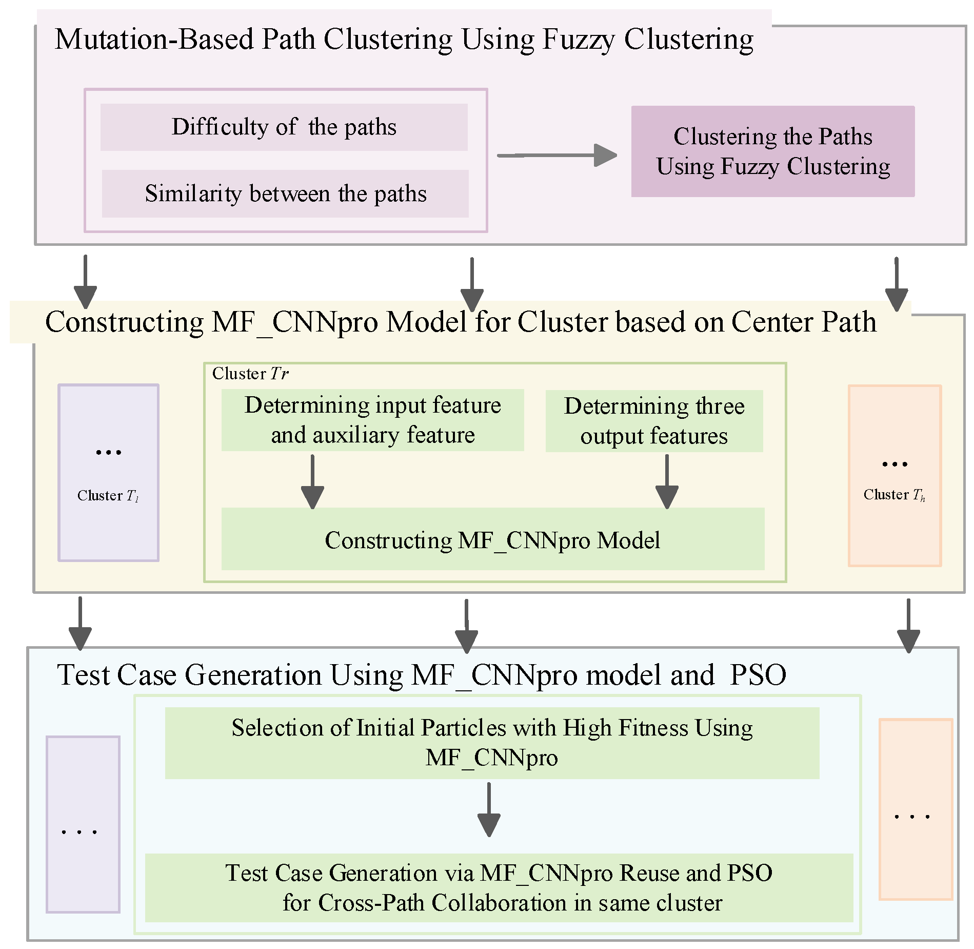
Figure 1. The framework of the proposed method.
Mathematics 14 00047 g001
Figure 2. The heatmap of the path similarity matrix.
Mathematics 14 00047 g002
Figure 3. CNNpro model [13].
Mathematics 14 00047 g003
Figure 4. our MF_CNNpro model.
Mathematics 14 00047 g004
Figure 5. The value of CP and SP.
Mathematics 14 00047 g005
Figure 6. The value of IA.
Mathematics 14 00047 g006
Figure 7. The value of U-Statistic.
Mathematics 14 00047 g007
Figure 8. The value of MSE.
Mathematics 14 00047 g008
Figure 9. The value of U.
Mathematics 14 00047 g009
Figure 10. Training Curves.
Mathematics 14 00047 g010
Figure 11. The success rates of test case generation methods.
Mathematics 14 00047 g011
Figure 12. The average number of iterations.
Mathematics 14 00047 g012
Figure 13. The average execution time.
Mathematics 14 00047 g013
Table 1. The absolute error value corresponding to path S 2 .
Input XPredicted Value Y ^ E ( X )
x 6 = ( 3 , 5 , 4 ) ( 0.71 , 0.02 , 0.94 ) 0.26
x 7 = ( 56 , 33 , 14 ) ( 0.06 , 0.2 , 0.2 ) 1.43
x 8 = ( 7 , 1 , 1 ) ( 0.38 , 0.06 , 0.54 ) 0.67
x 9 = ( 2 , 6 , 10 ) ( 0.2 , 0.01 , 0.36 ) 1.1
x 10 = ( 36 , 71 , 80 ) ( 0.59 , 0 , 0.99 ) 0.11
Table 2. The absolute error value corresponding to path S 5 .
Input XPredicted Value Y ^ E ( X )
x 6 = ( 3 , 5 , 4 ) ( 0.71 , 0.02 , 0.94 ) 0.42
x 10 = ( 36 , 71 , 80 ) ( 0.59 , 0 , 0.99 ) 0.32
x 11 = ( 31 , 60 , 59 ) ( 0.64 , 0 , 0.99 ) 0.37
x 12 = ( 52 , 71 , 45 ) ( 0.62 , 0 , 0.99 ) 0.35
x 13 = ( 17 , 22 , 9 ) ( 0.48 , 0 , 0.97 ) 0.37
Table 3. Detailed information of the program under test.
IDProgramLinesStatement Under TestFunctionNon-Equivalent MutantPaths
P1Triangle2617Triangle Classification349
P2Cal6822Date Calc449
P3Number27672Data Analysis14224
P4Energy2312112Energy Analysis33034
P5Supply9533206Material Flow1030113
P6monitor11,935320System Monitoring1640136
Table 4. Clustering Rate (CR) Comparison.
IDSC (%)NO-SC (%)Clustering Rate Difference (pp)
P122.0024.32−2.32
P255.5658.00−2.44
P350.0054.10−4.10
P419.4122.90−3.49
P516.7827.78−11.00
P615.3820.00−4.62
Avg29.8634.52−4.66
Table 5. U Test Significance Rate for Execution Time and Iterations.
IterationsExecution Time
MF_CNNpro+PSOpro
vs.
PSO(%)
MF_CNNpro+PPSOpro
vs.
PSO(%)
MF_CNNpro+PSOpro
vs.
PSO(%)
MF_CNNpro+PPSOpro
vs.
PSO(%)
p191.4093.73100.00100.00
p286.2087.7091.3293.28
p373.5376.4782.3594.12
p498.6095.8196.1097.60
p583.5089.3289.5093.71
p687.3091.1590.6094.68
Ave.86.7589.0391.6595.56
Disclaimer/Publisher’s Note: The statements, opinions and data contained in all publications are solely those of the individual author(s) and contributor(s) and not of MDPI and/or the editor(s). MDPI and/or the editor(s) disclaim responsibility for any injury to people or property resulting from any ideas, methods, instructions or products referred to in the content.