Article

Decoding Mouse Visual Tasks via Hierarchical Neural-Information Gradients

National Engineering Research Center for Multimedia Software, School of Computer Science, Wuhan University, Wuhan 430072, China
*
Authors to whom correspondence should be addressed.
Mathematics 2026, 14(1), 31; https://doi.org/10.3390/math14010031 (registering DOI)
Submission received: 18 November 2025 / Revised: 17 December 2025 / Accepted: 18 December 2025 / Published: 22 December 2025
(This article belongs to the Special Issue Machine Learning and Mathematical Methods in Computer Vision)

Abstract

Understanding how the brain encodes and decodes dynamic neural responses to visual stimuli is crucial for revealing visual information representation. Currently, most methods (including deep neural networks, DNNs) often overlook the dynamic generation process of neural data, such as hierarchical visual data, within the brain’s structure. In this work, we introduce two decoding paradigms: fine-grained decoding tests (single brain regions) and coarse-grained decoding tests (multiple regions). Using the Allen Institute’s Visual Coding Neuropixel dataset, we propose the Adaptive Topological Vision Transformer (AT-ViT), which exploits a biologically calibrated cumulative hierarchy derived from single-area decoding performance to adaptively decode topological relationships across brain regions. Extensive experiments confirm the ‘Information-Gradient Hypothesis’: single-area decoding accuracy should recovers the anatomical visual hierarchy, and AT-ViT achieves maximal performance when this data-driven gradient is respected. AT-ViT outperforms non-hierarchical baselines (ada-PCA/SVM) by 1.08–1.93% in natural scenes and 2.46–3.34% in static gratings across sessions, peaking at hierarchy 3 (visual cortex + thalamus/midbrain) with up to 96.21%, but declining 1–2% when including hippocampus data, highlighting its random, performance-hindering nature. This work demonstrates hierarchical networks’ superiority for brain visual tasks and opens avenues for studying hippocampal roles beyond visual decoding.

1. Introduction

The encoding and decoding mechanisms of dynamic neural responses to different visual stimuli can promote the generation of intelligent behaviors similar to human beings in machines. In the field of neuroscience, the visual system is mainly used to receive a large amount of sensory input from the external world. After the complex organization of these inputs in different regions of the brain, it can participate in more high-level cognitive functions [1]. The transmission process of visual stimuli in the brain is roughly from the retina to the thalamus, then to the primary visual cortex [2], and finally through two pathways to the anterior prefrontal nucleus (APN) [3,4] and the hippocampus [5]. Therefore, clarifying how visual information is encoded and decoded by a hierarchical structure has an important impact on understanding the computational principles of the visual system.
Visual stimuli are mainly transmitted in the brain in the form of neural impulses or electrical signals. These signals are processed through a dual-scale hierarchical framework that integrates well-established micro-architectures within individual areas into the broader, inter-areal visual hierarchy. At the micro-scale, within V1 and extrastriate cortices, laminar-specific computations generate specialized feature representations, such as pathway-dependent spatial frequency tuning across layers [6], layer-specific orientation suppression networks [7], and segregated coding of luminance increments in superficial layers versus decrements in deep layers [8]. At the macro-scale, the outputs of these intra-areal microcircuits are progressively pooled and transformed along the established ventral and dorsal streams. These well-documented laminar micro-architectures therefore do not function in isolation; rather, they supply the fine-grained, feature-selective streams that are hierarchically integrated at successive inter-areal processing stages, instead of treating entire cortical areas as functionally uniform entities. In encoding, the neural responses of the brain to external stimulus, such as natural scenes and videos [1,9], etc., are mainly studied from a neurobiological perspective. In decoding, models are established through technical means to solve object classification tasks [10] and pixel-level image reconstruction tasks [11], etc. In existing visual decoding schemes, there are mainly studies on decoding neural data collected from a single brain region, such as the primary visual cortex [12], which is rich in important visual information, and other multiple brain regions [1], as well as overall studies on neural data collected across brain regions [13]. However, this mode-separated research paradigm is still a limited explored field for understanding how neurons distributed in different brain regions represent natural scenes and the hierarchical structure and topological relationships of the brain itself. Given the complexity of visual processing at both within local microcircuits (intra-areal) and across the visual cortical hierarchy (inter-areal), we adopt the central hypothesis of this work, termed the Information-Gradient Hypothesis: the information content of neural activity in the visual system regarding external stimuli can be effectively quantified by the accuracy of algorithmic decoding; that is, the algorithmic decoding accuracy from individual brain regions quantitatively reflects their position in the visual processing hierarchy. We test and confirm this hypothesis using the Allen Neuropixels dataset. By analyzing the relationships among neural populations across different visual areas, as well as their relationship to external sensory inputs, we can gain deeper computational insights into the structure and representational properties of neural population codes. This constitutes the primary motivation for our decoding-based investigation of the visual system.
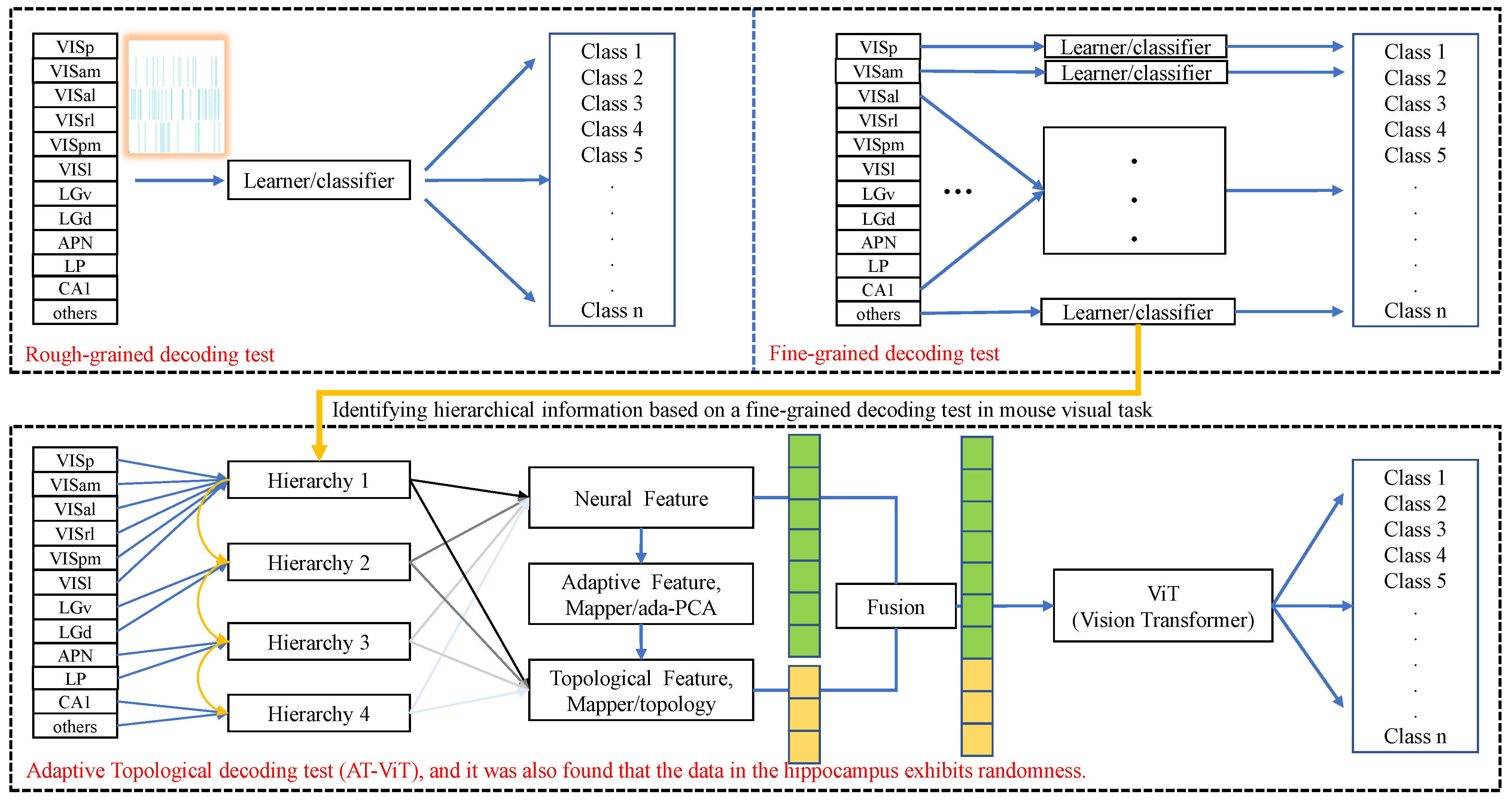
In this study, we utilized the Neuropixel dataset from the Allen Institute for Brain Science [14], which contains the spike responses of hundreds of neurons from the mouse visual cortex and some subcortical brain regions. The main visual tasks were to decode the corresponding external visual stimuli, such as natural scenes and static gratings, from the neural data. Decoding neural data from a single brain region was defined as fine-grained decoding tests, while decoding neural data across brain regions was defined as coarse-grained decoding tests. In Figure 1, we proposed an adaptive topological decoding method that uses deep network technology to explore the topological relationships of hierarchical visual data. The main contributions are as follows: (1) We perform fine-grained decoding of neural population activity from individual brain regions and quantified the task-relevant visual information content in each region by its single-area decoding, i.e., classification accuracy. (2) We propose a hybrid quantitative-anatomical pipeline that combines data-driven ranking from single-area decoding with anatomical calibration to construct biologically interpretable hierarchies. Subsequently, we propose an adaptive topological method (AT-ViT) that contains the hierarchical structure for decoding this cross-regional neural data. (3) We also find that the neural data collected from the hippocampus may even negatively impact performance enhancement. This finding is different from other studies that fuse data from various brain regions, and the specific role of hippocampal data with random decoding performance still holds significant scientific value.
Finally, we validated the effectiveness of the proposed method through comprehensive experiments. Furthermore, this study introduces a new avenue for discussion regarding the utilization of hierarchical deep networks as a tool to elucidate the computational principle of the mouse visual system. We also hope that this work can provide a new perspective for the field of biological vision to simultaneously apply hierarchical model structures and hierarchical data structures, such as brain’s visual structures and brain’s visual data.

2. Related Work

2.1. Hierarchical Processing in/for the Mouse Visual System

Generally, brain visual data is initially encoded in retinal ganglion cells and further processed through encoding and decoding in the lateral geniculate nucleus (LGN) and primary visual cortex (V1). These representations are then further processed in higher visual areas to extract increasingly abstract and meaningful information that supports learning and memory [1,11]. Consistent with the hierarchical organization of the visual system, temporal response latencies increase along the hierarchy, with higher-level regions exhibiting slower dynamics [15,16]. These observations suggest that the amount of visual information encoded or captured in brain structures follows a hierarchical organization principle. In recent years, deep neural networks (DNNs) have become invaluable tools in neuroscience for decoding visual representations from mouse brain recordings [17,18], bridging hierarchical processing principles with computational models. Benchmarks such as the SENSORIUM 2023 competition have established standardized evaluations of dynamic DNNs for predicting large-scale responses in mouse primary visual cortex (VISp) to natural videos [19]. These advancements extend to recurrent and dynamic encoding models, which capture the hierarchical temporal integration observed along the mouse visual pathway [20] and enable accurate reconstruction of dynamic visual scenes from V1 activity [21]. However, although these works clearly reveal empirical hierarchical processing, they typically do not exploit this information gradient, reflected in single-area decoding performance, as an explicit structural prior in multi-region models.

2.2. Fine-Coarse-Grained and Graph-Based Methods for Brain Network Decoding

In the neuroscience research paradigm, brain topology studies for neural decoding mainly focus on static graph construction [22,23] and dynamic graph construction [24,25]. Among them, static graph construction using anatomical connectivity matrices does not explicitly model the dynamic inter-dependencies between different regions of interest (ROIs) and is difficult to generalize in an end-to-end manner to different downstream tasks [13]. However, dynamic construction holds significant value for studying brain functions with time-varying characteristics. Then, the Allen Brain Observatory Datasets, with rich visual tasks and high spatiotemporal resolution from Neuropixels probes, can be used to study single brain regions with rich visual information in fine- and coarse-grained decoding paradigms, such as the VISp [12], as well as the visual hierarchy across multiple brain regions (from thalamus, visual cortex to hippocampus) [1]. In addition, graph neural networks (GNNs) have been widely applied to brain network analysis and cross-region prediction, as demonstrated by benchmarks like BrainGB [26]. Recent work has explored multimodal graph learning in neural systems, e.g., deep graph learning for multimodal brain networks with clinical signatures [27], although explicit multi-scale graph frameworks remain less explored. However, these studies focus mainly on information processing in single brain regions and topological processing in multiple brain regions, seemingly neglecting collaborative processing between single- and multi-region scales.

2.3. Hippocampal Roles and Our Presented Work in Visual Decoding and Beyond

In addition, in the field of neural decoding, multiple studies confirmed that mouse visual cortex regions may represent semantic features of learned visual categories [14,28]. Beyond visual coding, the hippocampus of rodents is believed to play a role in learning and memory similar to that of primates [29]. Regarding the function of the hippocampus, DNN-based analyses suggest hippocampal neurons contain less pixel-level information than thalamic or cortical ones [1], encoding abstract concepts instead [30]. In our study, we also found that neural data collected from the hippocampus under identical conditions impairs category decoding of visual tasks, consistent with the random baseline. To our knowledge, the present study is among the earliest to transform the observed relationship “single-area decoding accuracy ≈ position in visual hierarchy” into an explicit, end-to-end learnable topological prior for multi-region visual decoding in the mouse brain, leveraging the proposed fine-coarse-grained joint paradigm and Adaptive Topological Vision Transformer (AT-ViT).

3. Method

3.1. Pre-Knowledge

3.1.1. Mapper Algorithm

The Mapper algorithm [31,32] is a core tool in topological data analysis (TDA), mainly serving as an integrated approach for dimensionality reduction and clustering of data. Its advantage lies in preserving the topological features of the data and being capable of constructing and visualizing the topological structure of high-dimensional data.
The basic steps behind Mapper are as follows [31]: (1) Map to a lower-dimensional space using a filter function F, such as uniform manifold approximation and projection (UMAP) [33], in a given brain’s visual data D. (2) Construct a cover ( U i ) i I . i is the ith interval in the total interval I. (3) For each interval U i , cluster the points in the preimage F 1 ( U i ) into sets C i , 1 , , C i , k i . k i is the kth cluster set in the ith interval. (4) Construct the graph whose vertices are the cluster sets and an edge exists between two vertices if two clusters share some points in common, which represents the topological structure of the data. The Mapper construction is formally defined as the standard four-step topological summarization: Let X R N × T be the ada-PCA-reduced population activity in a given hierarchy tier. Filter function: F = U M A P : X R 2 . Cover: the filter space R 2 is covered by the pullback of a regular 10 × 10 grid of axis-aligned rectangles, each with 10% overlap in both directions, producing exactly 100 overlapping intervals U i . Local clustering: single-linkage clustering in each F 1 ( U i ) using OPTICS algorithm. Graph: 1-skeleton where n o d e s = c l u s t e r s , edges exist between two nodes if their clusters share at least one neuron-time point. It should also be noted that the Mapper graph is formally interpreted as the 1-skeleton of a simplicial complex: nodes represent 0-simplices (clusters), and edges represent 1-simplices between clusters that share at least one point. Higher-dimensional simplices are not constructed in our analysis because the 1-dimensional simplicial complex (graph) produced by the Mapper algorithm is sufficient to describe our current data. This is consistent with standard Mapper applications, where high-dimensional neural activity patterns are reduced to a 1-dimensional graph representation capturing their coarse topological structure.

3.1.2. Maximum Likelihood Estimate for PCA (ada-PCA)

Principal Component Analysis (PCA) is a commonly used data dimensionality reduction technique. Its advantages lie in the fact that by retaining the main components, it can filter out noise in the data for data preprocessing. To overcome the drawback of traditional PCA that requires manual specification of the number of principal components, an automatic method for selecting the dimension of PCA has been proposed [34]. This method, through Bayesian model selection [35,36], can automatically select the most appropriate number of principal components or the optimal parameters based on the consideration of model complexity and the amount of data.
We adopted the method proposed in [34], which we refer to as ada-PCA here. Through Bayesian model selection techniques, the n-dimensional sample set D = ( s 1 , s 2 , , s n ) is automatically reduced to an m-dimensional sample set D = ( s 1 , s 2 , , s m ) . s k refers to the neural data collected by the kth moment in the brain’s visual data.

3.1.3. Random Baseline in Mouse Visual Classification

A defined random baseline (Rb), or random accuracy, is mainly used to evaluate whether the model is above the correct prediction in a classification. Here, each class-label is assumed to be independent. The formula is as follows:
R b = 1 n
where R b is an abbreviation for random baseline and n refers to the number of classification labels in the classification task.

3.2. Adaptive Topology Vision Transformer (AT-ViT)

3.2.1. Coarse-Grained Decoding Tests

The coarse-grained decoding described in Figure 2 refers to the process where the neural data collected from each brain region are sent together to the constructed model for processing. This approach is often used when it is necessary to explore the hierarchical relationships or topological structures among brain’s visual system, as each brain region contains different amounts of information, resulting in a hierarchical relationship. As shown in the figure, the neural data collected from the visual cortex (VISp, VISam, VISal, VISrl, VISpm, VISl), thalamus/midbrain (LGv, LGd, APN, LP), and hippocampus (CA1, CA3, DG, SUB) are the firing data of the brain under visual stimulation, which have a one-to-one correspondence with the visual stimuli. Therefore, if all the neural data are sent to the model together, the trained model will be able to extract more visual information from the data to decode the visual stimuli. However, this method may overlook the generation process and firing mechanism of the visual system.

3.2.2. Fine-Grained Decoding Tests

The fine-grained decoding described in Figure 2 refers to the fact that the neural data collected from each brain region will be sent to the constructed model for processing, respectively. This method is often used to explore the amount of information contained in each brain region. Generally speaking, in visual decoding tasks, the brain region VISp in the visual cortex is the neural data we commonly use because it is the primary cortex of the visual system, and almost all the information transmitted to the visual cortex passes through the primary cortex. Due to the hierarchical organization of the brain’s visual system, that is, each brain region may only extract or process part of the information from the visual stimuli. Therefore, in addition to the VISp, the study of neural data from other brain regions is of great value.
Figure 2. Three methods are presented, namely coarse-grained decoding tests, fine-grained decoding tests, and Adaptive Topological decoding. In coarse-grained decoding tests, the focus is mainly on the topological analysis of brain’s visual data. In fine-grained decoding tests, the emphasis is on the detailed information mining of each brain region. Adaptive Topological decoding essentially incorporates the ideas of the first two modes. Since the hierarchical brain’s visual structure generates hierarchical brain’s visual data, the important information extracted in fine-grained decoding tests can usually reveal this hierarchical structure. Based on this, the Adaptive Topological decoding model is proposed to handle hierarchical visual data in the brain’s visual tasks.
Mathematics 14 00031 g002
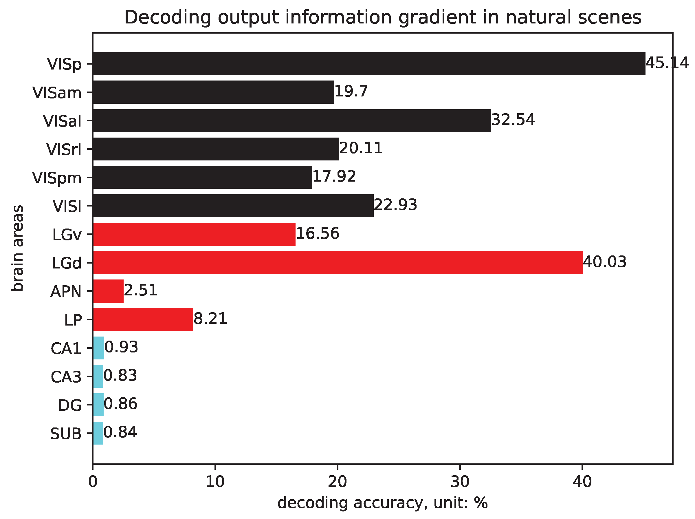
To better assess the amount of visual information contained in each brain region, we decoded the neural data collected from each brain region independently using the same SVM. These single-area decoding accuracies serve as a quantitative proxy for stimulus-related information content. We posit the following testable hypothesis (termed the Information-Gradient Hypothesis): In a hierarchically organized sensory system such as the mouse visual pathway, the amount of task-relevant visual information carried by different brain areas forms a graded continuum that mirrors the known anatomical and functional hierarchy. Consequently, when identical decoding algorithms are applied to individual areas, their standalone classification performance should recover this biological hierarchy in a monotonic fashion: retina → primary thalamus → visual cortex → secondary thalamus/midbrain → hippocampus. This hypothesis makes two strong, falsifiable predictions: (1) single-area decoding accuracy ranks the areas in the same order as the established visual processing hierarchy; (2) systematically incorporating areas from higher to lower tiers progressively improves multi-region decoding until the inclusion of near-random areas (e.g., hippocampus) degrades performance. As shown in the experiment of Figures 5 and 6, both predictions are strongly confirmed in the present dataset across all seven sessions and both visual tasks. This data-driven gradient calibrated to anatomical pathway is then directly used to construct the adaptive topological input for AT-ViT.

3.2.3. Adaptive Topological Decoding

The hierarchical input structure for AT-ViT is constructed using a hybrid quantitative-anatomical cumulative procedure (detailed in Section 3.2.4) that primarily ranks brain areas by session-averaged single-area decoding accuracy but calibrates thresholds to respect the known four-stage anatomical progression of the mouse visual pathway. This cumulative gradient enables adaptive topological fusion.
In Figure 2, the adaptive topological decoding test (AT-ViT) describes that the neural data collected from each brain region will be assigned to a hierarchical structure and then sent to the constructed model for processing. Here, this assigned hierarchical structure is mainly based on the amount of visual information observed in fine-grained decoding tests. Each hierarchy contains the neural data of several brain regions. It can be seen from the figure or the experimental results that hierarchy 1 mainly includes the brain regions of the visual cortex, hierarchy 2 includes the visual cortex and thalamus/midbrain (LGv, LGd), hierarchy 3 mainly includes the visual cortex and thalamus/midbrain, and hierarchy 4 includes the visual cortex, thalamus/midbrain, and hippocampus. In each hierarchy, the neural data will be adaptively dimensionally reduced and then the topological features will be extracted through the Mapper algorithm. These topological features and neural data are fused and sent to the Vision Transformer (ViT) model, attempting to absorb these hierarchical neural data through a hierarchical deep network. Here, the fusion mechanism (neural features and topological features) is defined as follows: for hierarchy tier n, let F n R N n × T be the neural activity and G n the Mapper graph (adjacency matrix A n { 0 , 1 } m n × m n , where m n is the number of clusters in tier n). The topological feature vector is the flattened upper triangle of A n (length m n 2 ). Neural and topological features are concatenated channel-wise, projected to dimension 64, and fed as patches to the V i T : z 0 = [ L i n e a r 64 ( F n v e c ( A n ) ) C L S ] + E p o s (where v e c is the vectorization operator, C L S is the class token, E p o s is the positional embedding). Finally, ViT embedding is formally described as standard ViT patch embedding with added C L S token and learnable positional encoding (hidden size 64, 6 layers, 32 heads).
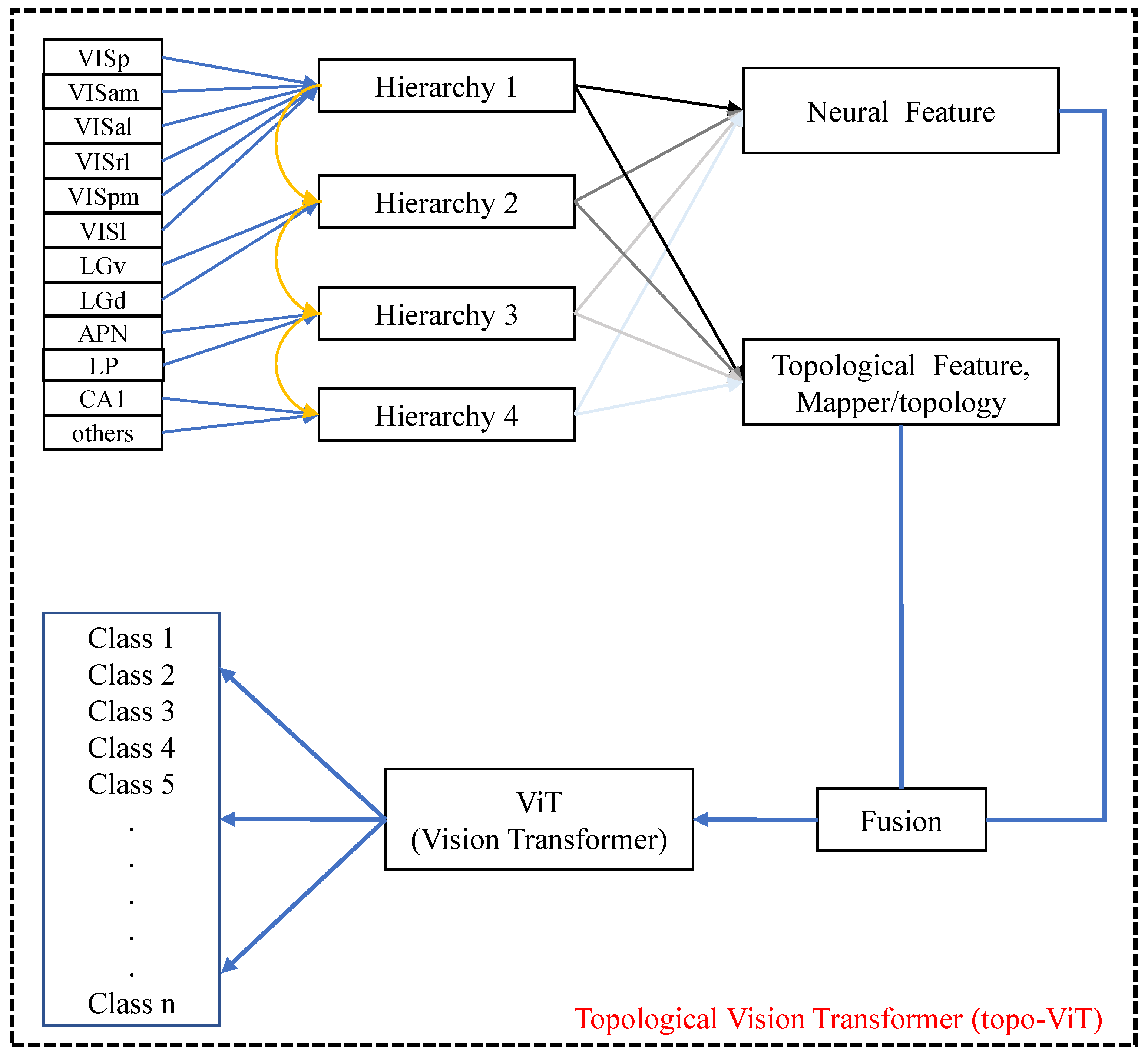
In Figure 3, the topological vision transformer (topo-ViT) describes that the neural data collected from each brain region will be assigned to a hierarchical structure and then sent to the constructed model for processing. Here, there is no adaptive dimensionality reduction processing. We attempt to directly extract topological features from the neural data and observe the decoding effect of this hierarchical deep network.

3.2.4. Quantitative Construction of the Information Hierarchy

The hierarchical input to AT-ViT is built in a cumulative manner using a hybrid approach that combines data-driven ranking from single-area decoding performance with anatomical calibration as follows.
  • For each session s and each brain area r, train an SVM and compute classification accuracy A c c r , s .
  • For each area r, compute its cross-session average accuracy
    A c c ¯ r = 1 S s = 1 S A c c r , s
    where S is the number of sessions.
  • Compute the normalized information score
    I n f o r = A c c ¯ r R b A c c ¯ VISp R b
    where R b is the random baseline, and VISp consistently shows the highest A c c ¯ r .
  • Sort all recorded areas by I n f o r in descending order.
  • Group them into n cumulative hierarchies using n 1 fixed relative thresholds T H n 1 . Hierarchy 1 contains areas with I n f o r T H 1 . Each higher hierarchy n ( n = 2 , 3 , 4 , ) cumulatively includes all areas from lower hierarchies plus the new areas falling into the corresponding I n f o r interval.
Specifically for this work, the selection of four hierarchical levels employs a hybrid quantitative-anatomical approach, where normalized information scores I n f o r , derived from session-averaged single-area decoding accuracies, serve as the primary data-driven basis for ranking and grouping brain areas, while thresholds are calibrated to align with the established four-stage anatomical progression in the mouse visual pathway (primary thalamus such as LGv/LGd → visual cortex → secondary thalamus/midbrain such as APN/LP → hippocampus). This calibration splits the thalamus into primary and secondary tiers based on I n f o r values (e.g., LGv/LGd sometimes exceeding or being close to lower visual cortex areas but grouped anatomically for biological plausibility, detailed in Section 4.4), ensuring the cumulative hierarchies respect both empirical performance gradients and known neuroanatomical structures. The resulting close alignment with the anatomical hierarchy strongly validates the information-gradient hypothesis, with the grouping ultimately driven solely by decoding accuracies. It is worth emphasizing that the hierarchy is data-dependent, as it emerges from the empirical decoding accuracies on the Allen Neuropixels dataset. However, it is model-independent, as similar information gradients (visual cortex > thalamus/midbrain > hippocampus) can be observed using different decoders, supporting the general validity of the Information-Gradient Hypothesis beyond our SVM proxy. Additionally, the resulting hierarchies are reported in this study in Table 1 and Table 2, Figure 4 and  Figure 5. They are directly used as the adaptive topological input to AT-ViT (see Algorithm 1).
Algorithm 1 AT-ViT Algorithm.
Input: brain’s visual data D = ( s 1 , s 2 , , s n )
Parameter: H i e r a r c h y = n , T r a n s f o r m e r l a y e r s = 6 , h e a d s = 32 , h i d d e n s i z e = 64 , l e a r n i n g r a t e = 1 × 10⁻³, f e e d f o r w a r d l a y e r s = 4 , e p o c h s = 30 , n = 1 , 2 , , j .
Output: AT-ViT model M
  1:
Initialize θ model parameters , optimizer. t 0 .
  2:
D n SVM ( D ) in fine-grained decoding tests
  3:
D t o p o {Mapper: ada-PCA, topology}( ( D n )
  4:
D f u s i o n Function F f u s i o n ( D n , D t o p o )
  5:
while  t e p o c h s   do
  6:
   while  Traversal on D f u s i o n is not completed  do
  7:
     Sample batch ( s 1 , s 2 , , s b ) D .
  8:
      E PatchEmbed ( s 1 , s 2 , , s b ) + PosEmbed .
  9:
     for  l = 1 T r a n s f o r m e r l a y e r s  do
10:
         E MultiHeadAttention ( E , h e a d s ) .
11:
         E FeedForward ( E , f e e d f o r w a r d l a y e r ) .
12:
     end for
13:
      L ^ Predict ( E ) .
14:
      L CrossEntropy ( L ^ , L true ) .
15:
      θ Update ( θ , θ L , l e a r n i n g r a t e ) .
16:
   end while
17:
    t t + 1 .
18:
end while
19:
return  M ( θ ) .

3.3. Algorithms and Listings

Before applying the AT-ViT, a hierarchical data structure needs to be extracted. In this work, the collected neural data can be observed to have a hierarchical structure in fine-grained decoding tests based on the amount of visual information, that is, there exists a hierarchical structure in the brain’s visual system. First, the neural data is processed through adaptive dimensionality reduction, and then the topological structure contained in the neural data is extracted through the Mapper algorithm. Finally, the neural data and topological feature are fused and fed into the hierarchical deep network. This hierarchical deep network is used to extract the hierarchical structure of the neural data.

4. Experiment

4.1. Dataset and Metric

The electrophysiological dataset we used is from Allen Brain Visual Coding [14], and its dataset and preprocessing code are in “https://allensdk.readthedocs.io/en/latest/visual_coding_neuropixels.html, (accessed on 10 December 2025)”. This dataset consists of 32 experimental sessions, each containing three hours of total experimental data, and the same protocol was used across different mice. These datasets include functional traces of individual spikes at the single-neuron level, which were recorded during multiple repeated trials of various natural (bears, trees, cheetahs, etc.) and artificial (drifting gratings, oriented bars, etc.) visual stimuli presented to the mice. In this work, we focus on two visual classification tasks: natural scenes and static gratings. For fine-grained decoding tests, seven sessions were used, such as (session_id) 761418226, 763673393, 773418906, 791319847, 797828357, 798911424, 799864342. Then, for the training, testing, and comparison with other methods of AT-ViT, two new sessions were used, such as (session_id) 760345702, 762602078. In this work, all evaluation metrics adopt a unified classification accuracy, that is,
A C C = 1 F c o u n t _ n o n z e r o ( Y p r e d i c t i o n Y l a b e l ) l e n ( Y p r e d i c t i o n ) ,
where F c o u n t _ n o n z e r o is a function for counting the non-zero elements in a vector, Y p r e d i c t i o n is the predicted value of sample Y, Y l a b e l is the true value of sample Y, and l e n ( Y p r e d i c t i o n ) is the total length of sample Y. Finally, 10-fold cross validation was used on the dataset to evaluate the model and verify the hypothesis. Given the highly balanced class distribution in both tasks (each category presented in ≈50 trials per session), accuracy is used as the primary metric. Our decoding-centric approach focuses on quantifying task-relevant visual information content across brain regions using algorithmic performance as a proxy; alternative classification metrics or deeper single-neuron analyses are valuable but lie beyond the current scope.

4.2. ada-PCA/SVM Decoding in Visual Tasks

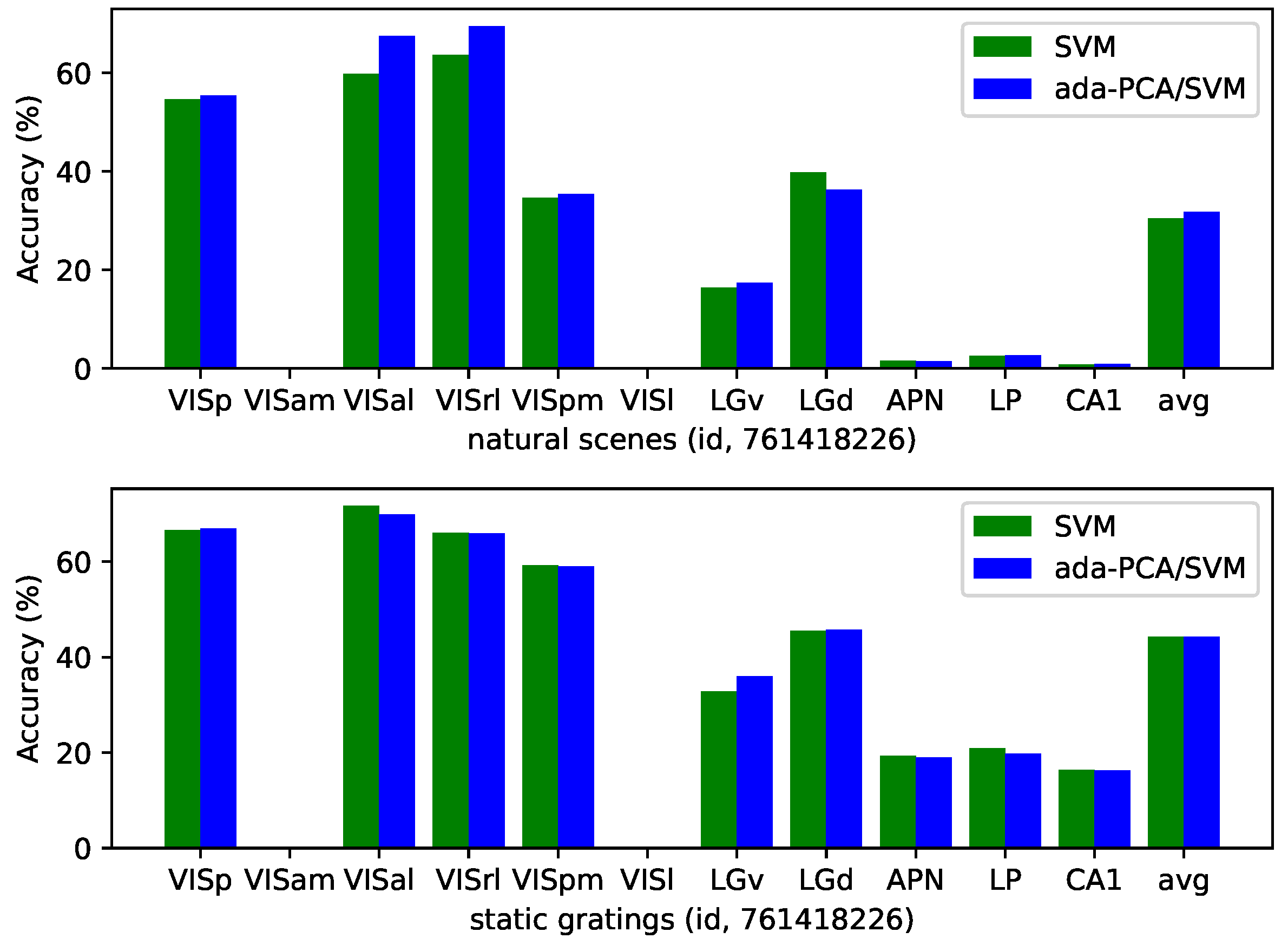
Figure 4 shows the decoding of brain’s visual data using the adaptive dimensionality reduction and Support Vector Machine (SVM). In natural scenes, the histogram indicates that the decoding performance of ada-PCA/SVM, which has the ability of adaptive dimensionality reduction, is significantly higher than that of SVM alone. Additionally, the decoding performance among different brain regions also reveals that the amount of information contained in their data varies. Specifically, the decoding performance of the visual cortex is significantly higher than that of the thalamus/midbrain, and the thalamus/midbrain’s performance is higher than that of the hippocampus. In static gratings, the decoding performance of ada-PCA/SVM is almost the same as that of SVM alone. In addition, the amount of information contained in each brain region shows a similar trend as in natural scenes.

4.3. Fine-Grained Decoding Tests in Visual Tasks

Table 1 is based on Figure 4, presenting a simple SVM algorithm’s performance in seven sessions and two visual tasks (i.e., natural scenes and static gratings), testing the amount of information contained in each brain region. The bold font indicates the highest decoding accuracy in each session and brain region. Moreover, to better evaluate the decoding performance and the amount of visual information in each brain region, a random decoding accuracy is used as a benchmark, i.e., the random baseline. If the decoding accuracy is close to the random baseline, the decoding of that brain region is equivalent to random guessing; if it is higher than the random baseline, the brain region contains more information. In natural scenes, it can be seen from the figure that the decoding accuracy of the visual cortex and thalamus/midbrain is significantly higher than the random baseline, while in the hippocampus, such as CA1, it is equivalent to the random baseline. This phenomenon is also reflected in the experimental results of static gratings. Similarly, in both natural scenes and static gratings, a hierarchical relationship regarding the amount of visual information can be observed based on the decoding performance, that is, the visual information in the visual cortex is higher than that in the thalamus/midbrain, and the visual information in the thalamus/midbrain is higher than that in the hippocampus.
To rigorously address whether hippocampal population activity contains task-relevant visual information, a one-sided Wilcoxon signed-rank test was performed against the random baseline in both tasks. For natural scenes (128 classes, R b = 0.78 ), the hippocampal accuracies across the seven sessions were 0.81, 0.79, 0.76, 0.97, 0.74, 1.71, and 0.76. For static gratings (6 classes, R b = 16.67 ), the accuracies were 16.36, 14.83, 16.21, 16.82, 16.85, 20.29, and 17.30. The test fails to reject the null hypothesis that the median accuracy is no better than random baseline (natural scenes: W = 18 , p = 0.289 ; static gratings: W = 15 , p = 0.469 ). Combined with the performance degradation observed in Figure 5 and Figure 6 when hippocampus is forcibly included in Hierarchy 4, these results provide strong statistical evidence that, under the present passive-viewing conditions, hippocampal population activity contains no decodable task-relevant visual information and behaves statistically indistinguishable from random noise with respect to stimulus category decoding.
Insight and discussion. Based on the above analysis of the visual information contained in each brain region, the decoding performance of brain’s visual data can reflect the hierarchical organization of the visual system. Based on this relationship, in fine-grained decoding tests, we can stratify brain’s visual data based on the amount of visual information. Additionally, the random decoding accuracy observed in the hippocampus indicates that the visual information in this brain region is very scarce. However, if there is still visual firing data in this brain region, can we assume that the neural data in this brain region might be a random guess?

4.4. Brain Hierarchy Setting and Experiment

Table 2 is derived from Table 1. In addition to single-area decoding performance, the hierarchical assignment also follows a cumulative scheme grounded in feedforward anatomical connectivity (retina → LGN → visual cortex → higher-order thalamus/midbrain → hippocampus). As follows in Figure 5, hierarchy 1: visual cortex (VISp, VISam, VISal, VISrl, VISpm, VISl); hierarchy 2: visual cortex + thalamus/midbrain 1 (LGv, LGd); hierarchy 3: visual cortex + thalamus/midbrain 2 (LGv, LGd, APN, LP); hierarchy 4: visual cortex + thalamus/midbrain + hippocampus (CA1, CA3, DG, SUB). Here, some brain regions in the thalamus/midbrain are, respectively, classified into hierarchy 2 and hierarchy 3, because the visual information contained in the brain regions LGv and LGd sometimes aligns with that of the visual cortex, but the visual information in APN, and LP is significantly less than that in the visual cortex. Generally, four cumulative hierarchy are formed by progressively adding brain areas according to a hybrid quantitative-anatomical criterion: brain areas are primarily ordered by decreasing single-area decoding accuracy (visual cortex first, followed by primary thalamic relays, then secondary thalamic/midbrain regions, and finally hippocampus), but thresholds are calibrated to respect the established four-stage anatomical progression of the mouse visual pathway. This ensures both empirical robustness and biological interpretability.
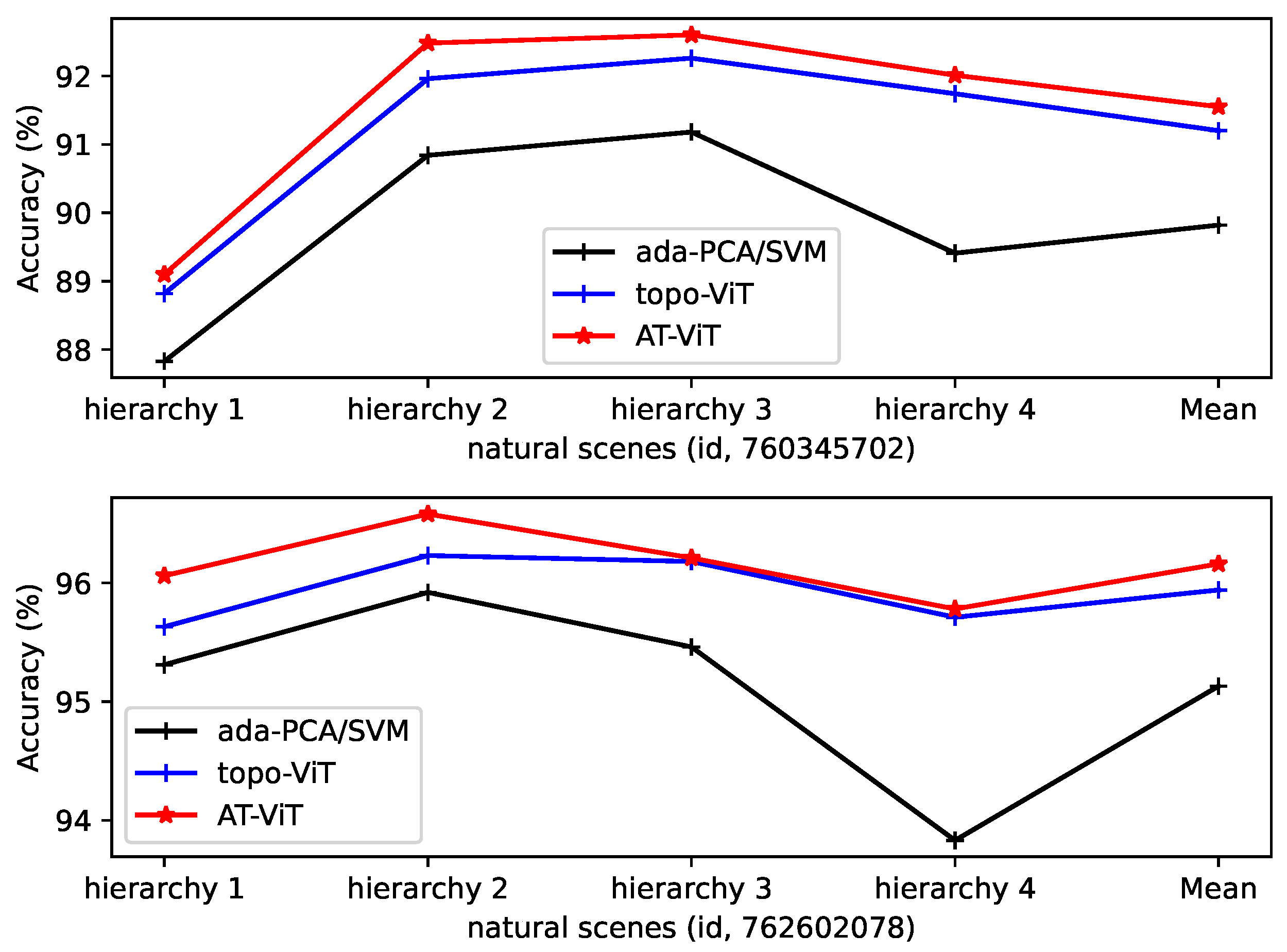
Table 3 is based on the division of the hierarchy according to visual information based on Table 2. The proposed method was trained, tested, compared and analyzed in two sessions. From the experimental results, the decoding performance of topo-ViT is higher than that of ada-PCA/SVM, with improvements of 1.54%, 2.47%, 0.85%, and 3.27% in natural scenes and static gratings, respectively. Additionally, the decoding performance of the proposed hierarchical networks (such as AT-ViT) is significantly higher than that of non-hierarchical methods (such as ada-PCA/SVM), with improvements of 1.93%, 2.46%, 1.08%, and 3.34% in natural scenes and static gratings, respectively. Overall, the performance of the proposed AT-ViT is also higher than that of topo-ViT. Finally, the decoding performance in hierarchy 1 and hierarchy 2 increases significantly, while in hierarchy 3, there is a slowdown trend, but in hierarchy 4, the performance significantly decreases. These results indicate that the hippocampus-related brain regions hurt the performance.

4.5. Decoding and Analyzing in Hierarchical Information Gradients

Figure 6 shows the classification accuracy curves of visual tasks in the decoding of visual hierarchical data. Hierarchical networks significantly outperform non-hierarchical networks. In session (760345702), as the hierarchy increases, the decoding performance gradually improves, but it drops in hierarchy 4. This indicates that the neural data from the hippocampus (with performance close to the random baseline) hurts the decoding performance. In session (762602078), as the hierarchy increases, the decoding performance decreases in both hierarchies 2, 3, and 4. The reasons can be analyzed in Table 1 and Table 2. The performance in brain region LP is generally higher than that in APN, and even the performance in APN approaches the random baseline, such as 0.82% and 16.66%. It can be seen from Table 2 that session (762602078) collected neural data from APN and LP, and session (760345702) only record the neural data from LP. These experimental results reveal that the visual information contained in the visual data of different visual regions is highly complementary and holds significant reference value for joint research on multiple brain regions. Based on these, the best decoding performance can be achieved when the hierarchical hyperparameter is set to n = 3 in this work. That is to say, the neural data collected in the hippocampus during visual tasks is similar to noise, which affects the decoding performance of visual classification. In addition, we believe that the exploration and verification of other functions of the hippocampus can be further studied using other relevant datasets.
Table 3. In the four hierarchical structures that have been divided, the proposed model and other models are subjected to relevant experiments and comparative analysis in the two selected sessions. Here, the symbol ↑ indicates that a higher decoding accuracy value is better.
Session_id (ada-PCA/SVM)Hierarchy 1Hierarchy 2Hierarchy 3Hierarchy 4Mean
(nat_Scenes/Static_Gra) ↑
76034570287.83/83.1990.84/84.7791.18/84.6589.41/82.2489.82 (0%)/83.71 (0%)
76260207895.31/85.2195.92/85.4295.46/84.1193.83/82.0695.13 (0%)/84.20 (0%)
session_id (topo-ViT)
76034570288.82/84.2391.96/86.4992.26/87.0791.74/85.3291.20 (1.54%)/85.78 (2.47%)
76260207895.63/87.4396.23/86.8496.18/86.9895.71/86.5395.94 (0.85%)/86.95 (3.27%)
session_id (AT-ViT)
76034570289.10/84.5192.48/86.0492.60/86.5792.01/85.9791.55 (1.93%)/85.77 (2.46%)
76260207896.06/87.2096.58/87.4496.21/87.1295.78/86.2696.16 (1.08%)/87.01 (3.34%)
Figure 6. The decoding accuracy maps for two sessions under natural scene conditions are presented. As the hierarchical level of selected visual regions increases, the decoding performance of various algorithms (e.g., ada-PCA/SVM, topo-ViT, and AT-ViT) consistently exhibits an initial rise followed by a decline. Overall, decoding performance peaks at hierarchy 3 (which includes visual cortex + thalamus/midbrain). After incorporating the hippocampus in hierarchy 4, performance drops substantially. Finally, the “Mean” metric represents the average decoding accuracy across hierarchy 1 to 4.
Mathematics 14 00031 g006

5. Discussion

5.1. The Proposed Model and Its Theoretical Discussion

This work mainly explores brain’s visual data from fine-grained decoding tests in a single brain region and coarse-grained decoding tests across brain regions. The adaptive topological method (AT-ViT) is a preliminary attempt, and there is still much room for improvement in its model. For example, more advanced algorithms can be adopted for hierarchical data and combined with the hierarchical functions of the visual system. Currently, graph networks have certain advantages [13], but these networks do not well consider the characteristics of brain’s visual system, that is, the generation process of hierarchical data. In the future, research on visual function can be conducted from the information attributes of visual data and the structural attributes of the visual system.
While this work is primarily empirical, we provide a brief theoretical motivation for AT-ViT’s hierarchical design using information theory. The Information-Gradient Hypothesis posits that single-area decoding accuracy A c c r proxies the mutual information M I ( s t i m u l u s ; a c t i v i t y r ) between visual stimulus and neural activity in area r. By sorting areas via I n f o r and cumulatively fusing tiers, AT-ViT maximizes the total M I ( s t i m u l u s ; d e c o d e d o u t p u t ) through progressive integration: lower tiers (high I n f o r ) capture core features, while higher tiers add complementary (but diminishing) information without redundancy. Formally, for a flat model, the entropy H ( o u t p u t ) may increase due to noise from low- I n f o r areas; in contrast, our cumulative scheme ensures Δ I n f o 0 per tier until random baseline, where including tier 4 (hippocampus) satisfies H ( o u t p u t s t i m u l u s ) H ( r a n d o m ) , degrading performance. In Equation (2), Δ A c c Δ H ( o u t p u t s t i m u l u s ) for random tiers, bounded by the channel capacity of the visual pathway. Rigorous bounds for hybrid AT-ViT models remain open and are suggested for future theoretical extensions.

5.2. Reinterpreting the Role of Hippocampal Signals in Visual Decoding

In the paper [1], it was also found that the collected data from the hippocampus (including CA1, CA3, DG, and SUB) for the decoding of complex pixel-level details in the stimuli is unreliable. They believe that this difference can be partially attributed to their position at the end of the visual pathway. In our study, we defined a random baseline as a reference, and found that the collected data from the hippocampus may have a negative impact on performance, that is, random guessing. This hypothesis has scientific value for future research on the function of the hippocampus. For example, the recent finding that visual working memory content is represented in primate V1 suggests that top-down signals from higher-order regions can substantially influence early visual activity [37]. Therefore, the seemingly random hippocampal signal in this work could reflect such task-irrelevant top-down modulation.

5.3. Generalizability and Broader Implications

The heuristic for hierarchical grouping, based on fixed thresholds applied to normalized decoding accuracies, is not limited to the mouse visual system. It can be directly applied to any layered system that generates hierarchical data with graded information content, including other sensory modalities (e.g., auditory or somatosensory pathways), motor hierarchies, decision-making cascades, or even artificial hierarchical networks. By using task-specific decoding performance as an empirical proxy for information gradients, researchers can systematically probe relationships between system structure and layered data representations without prior anatomical knowledge, thereby extending our Information-Gradient Hypothesis beyond vision in hierarchical biological or artificial systems.

6. Conclusions

This work provides direct empirical support for the Information-Gradient Hypothesis by showing that stimulus decoding performance from single brain areas reliably recapitulates the known hierarchical organization of the mouse visual system; it achieves this through a multi-scale analysis of neural data, ranging from fine-grained decoding tests within regions to coarse-grained decoding tests across regions, leading to a hierarchical classification based on visual information (or decoding outcomes). The proposed adaptive topological Vision Transformer (AT-ViT) initially addresses this hierarchical data and demonstrates the superiority of hierarchical networks in brain’s visual data, mainly through adaptive dimensionality reduction and extraction of topological features to process visual data. Since brain’s visual data originates from the hierarchical organization of the visual system, the amount of information contained in each brain region may vary, which has been proven in the experiment. In addition, this study found that the neural data collected in the hippocampus may have a random baseline for decoding, which has a negative impact on decoding performance across brain regions. However, the specific function and firing mechanism of this hippocampal data with a random baseline still needs further research.
In addition to the advances presented, this study also has several limitations. Most of the models developed in this work were primarily designed to validate the hypothesis and to perform decoding analyses on visual neural data, whereas relatively few fine-grained models were developed to explicitly represent and compare the generative mechanisms underlying visual processing. These limitations highlight the need for future improvements in model’s interpretability.

Author Contributions

Conceptualization, J.F.; Methodology, J.F.; Software, J.F. and X.F.; Validation, Y.L. and J.L.; Formal analysis, J.F. and X.F.; Resources, Y.L. and J.L.; Writing—original draft, J.F.; Writing—review and editing, X.F. and Y.L.; Visualization, J.F. and X.F.; Supervision, Y.L. and J.L.; Funding acquisition, Y.L. and J.L. All authors have read and agreed to the published version of the manuscript.

Funding

This research was funded by National Natural Science Foundation of China (62372335); National Natural Science Foundation of China (U23A20318); National Natural Science Foundation of China (62276195); Science and Technology Major Project of Hubei Province (2024BAB046); and Innovative Research Group Project of Hubei Province (2024AFA017).

Data Availability Statement

The original contributions presented in this study are included in the article. Further inquiries can be directed to the corresponding authors.

Conflicts of Interest

The authors declare no conflicts of interest.

References

  1. Chen, Y.; Beech, P.; Yin, Z.; Jia, S.; Zhang, J.; Yu, Z.; Liu, J.K. Decoding dynamic visual scenes across the brain hierarchy. PLoS Comput. Biol. 2024, 20, e1012297. [Google Scholar] [CrossRef]
  2. Hubel, D.; Wiesel, T. Receptive fields, binocular interaction and functional architecture in the cat’s visual cortex. J. Physiol. 1962, 160, 106–154. [Google Scholar] [CrossRef]
  3. Lui, F.; Gregory, K.M.; Blanks, R.H.I.; Giolli, R.A. Projections from visual areas of the cerebral cortex to pretectal nuclear complex, terminal accessory optic nuclei, and superior colliculus in macaque monkey. J. Comp. Neurol. 1995, 363, 439–460. [Google Scholar] [CrossRef] [PubMed]
  4. Giber, K.; Slézia, A.; Bokor, H.; Bodor, Á.L.; Ludányi, A.; Katona, I.; Acsády, L. Heterogeneous output pathways link the anterior pretectal nucleus with the zona incerta and the thalamus in rat. J. Comp. Neurol. 2007, 506, 122–140. [Google Scholar] [CrossRef]
  5. Turk-Browne, N.B. The Hippocampus as a Visual Area Organized by Space and Time: A Spatiotemporal Similarity Hypothesis. Vis. Res. 2019, 165, 123–130. [Google Scholar] [CrossRef]
  6. Wang, T.; Dai, W.; Wu, Y.; Li, Y.; Yang, Y.; Zhang, Y.; Zhou, T.; Sun, X.; Wang, G.; Li, L.; et al. Nonuniform and pathway-specific laminar processing of spatial frequencies in the primary visual cortex of primates. Nat. Commun. 2024, 15, 4005. [Google Scholar] [CrossRef] [PubMed]
  7. Wang, T.; Li, Y.; Yang, G.; Dai, W.; Yang, Y.; Han, C.; Wang, X.; Zhang, Y.; Xing, D. Laminar Subnetworks of Response Suppression in Macaque Primary Visual Cortex. J. Neurosci. 2020, 40, 7436–7450. [Google Scholar] [CrossRef]
  8. Yang, Y.; Wang, T.; Li, Y.; Dai, W.; Yang, G.; Han, C.; Wu, Y.; Xing, D. Coding strategy for surface luminance switches in the primary visual cortex of the awake monkey. Nat. Commun. 2022, 13, 286. [Google Scholar] [CrossRef] [PubMed]
  9. Karamanlis, D.; Schreyer, H.M.; Gollisch, T. Retinal Encoding of Natural Scenes. Annu. Rev. Vis. Sci. 2022, 8, 171–193. [Google Scholar] [CrossRef]
  10. Wen, H.; Shi, J.; Zhang, Y.; Lu, K.H.; Cao, J.; Liu, Z. Neural Encoding and Decoding with Deep Learning for Dynamic Natural Vision. Cereb. Cortex 2018, 28, 4136–4160. [Google Scholar] [CrossRef]
  11. Zhang, Y.; Jia, S.; Zheng, Y.; Yu, Z.; Tian, Y.; Ma, S.; Huang, T.; Liu, J.K. Reconstruction of natural visual scenes from neural spikes with deep neural networks. Neural Netw. 2020, 125, 19–30. [Google Scholar] [CrossRef]
  12. Iqbal, A.; Dong, P.; Kim, C.M.; Jang, H. Decoding Neural Responses in Mouse Visual Cortex through a Deep Neural Network. In Proceedings of the 2019 International Joint Conference on Neural Networks (IJCNN), Budapest, Hungary, 14–19 July 2019; pp. 1–7. [Google Scholar] [CrossRef]
  13. Li, Z.; Li, Q.; Zhu, Z.; Hu, Z.; Wu, X. Multi-Scale Spatio-Temporal Fusion With Adaptive Brain Topology Learning for fMRI Based Neural Decoding. IEEE J. Biomed. Health Inform. 2024, 28, 262–272. [Google Scholar] [CrossRef]
  14. Siegle, J.; Jia, X.; Durand, S.; Gale, S.; Bennett, C.; Graddis, N.; Heller, G.; Ramirez, T.; Choi, H.; Luviano, J.; et al. Survey of spiking in the mouse visual system reveals functional hierarchy. Nature 2021, 592, 86–92. [Google Scholar] [CrossRef]
  15. Harris, J.A.; Mihalas, S.; Hirokawa, K.E.; Whitesell, J.D.; Choi, H.; Bernard, A.; Bohn, P.; Caldejon, S.; Casal, L.; Cho, A.; et al. Hierarchical organization of cortical and thalamic connectivity. Nature 2019, 575, 195–202. [Google Scholar] [CrossRef]
  16. D’Souza, R.D.; Wang, Q.; Ji, W.; Meier, A.M.; Kennedy, H.; Knoblauch, K.; Burkhalter, A. Hierarchical and nonhierarchical features of the mouse visual cortical network. Nat. Commun. 2022, 13, 106–154. [Google Scholar] [CrossRef]
  17. Cadena, S.A.; Sinz, F.H.; Muhammad, T.; Froudarakis, E.; Cobos, E.; Walker, E.Y.; Reimer, J.; Bethge, M.; Tolias, A.; Ecker, A.S. How Well Do Deep Neural Networks Trained on Object Recognition Characterize the Mouse Visual System? In Proceedings of the 33rd Conference on Neural Information Processing Systems (NeurIPS 2019), Vancouver, BC, Canada, 8–14 December 2019. [Google Scholar]
  18. Steinmetz, N.A.; Zatka-Haas, P.; Carandini, M.; Harris, K.D. Distributed coding of choice, action and engagement across the mouse brain. Nature 2019, 576, 266–273. [Google Scholar] [CrossRef] [PubMed]
  19. Turishcheva, P.; Fahey, P.G.; Vystrčilová, M.; Hansel, L.; Froebe, R.; Ponder, K.; Qiu, Y.; Willeke, K.F.; Bashiri, M.; Baikulov, R.; et al. Retrospective for the Dynamic Sensorium Competition for predicting large-scale mouse primary visual cortex activity from videos. In Proceedings of the Advances in Neural Information Processing Systems; Globerson, A., Mackey, L., Belgrave, D., Fan, A., Paquet, U., Tomczak, J., Zhang, C., Eds.; Curran Associates, Inc.: Red Hook, NY, USA, 2024; Volume 37, pp. 118907–118929. [Google Scholar] [CrossRef]
  20. Rudelt, L.; Marx, D.G.; Spitzner, F.P.; Cramer, B.; Zierenberg, J.; Priesemann, V. Signatures of hierarchical temporal processing in the mouse visual system. PLoS Comput. Biol. 2024, 20, e1012355. [Google Scholar] [CrossRef] [PubMed]
  21. Bauer, J.; Margrie, T.W.; Clopath, C. Movie reconstruction from mouse visual cortex activity. eLife 2025. [Google Scholar] [CrossRef]
  22. Zhang, H.; Song, R.; Wang, L.; Zhang, L.; Wang, D.; Wang, C.; Zhang, W. A dynamic graph convolutional neural network framework reveals new insights into connectome dysfunctions in ADHD. NeuroImage 2022, 246, 118774. [Google Scholar] [CrossRef]
  23. Zhang, H.; Song, R.; Wang, L.; Zhang, L.; Wang, D.; Wang, C.; Zhang, W. Classification of Brain Disorders in rs-fMRI via Local-to-Global Graph Neural Networks. IEEE Trans. Med Imaging 2023, 42, 444–455. [Google Scholar] [CrossRef] [PubMed]
  24. Kim, B.H.; Ye, J.C.; Kim, J.J. Learning Dynamic Graph Representation of Brain Connectome with Spatio-Temporal Attention. In Proceedings of the 34rd Conference on Neural Information Processing Systems (NeurIPS 2021), Virtual, 6–14 December 2021; Curran Associates, Inc.: Red Hook, NY, USA, 2021; pp. 4314–4327. [Google Scholar]
  25. El-Gazzar, A.; Thomas, R.M.; van Wingen, G. Dynamic adaptive spatio-temporal graph convolution for fMRI modelling. In Proceedings of the Machine Learning in Clinical Neuroimaging: 4th International Workshop, Strasbourg, France, 27 September 2021; pp. 125–134. [Google Scholar] [CrossRef]
  26. Cui, H.; Dai, W.; Zhu, Y.; Kan, X.; Gu, A.A.; Lukemire, J.; Zhan, L.; He, L.; Guo, Y.; Yang, C. BrainGB: A Benchmark for Brain Network Analysis with Graph Neural Networks. IEEE Trans. Med. Imaging 2023, 42, 493–506. [Google Scholar] [CrossRef] [PubMed]
  27. Jiao, Y.; Zhao, K.; Wei, X.; Carlisle, N.B.; Keller, C.J.; Oathes, D.J.; Fonzo, G.A.; Zhang, Y. Deep graph learning of multimodal brain networks defines treatment-predictive signatures in major depression. Mol. Psychiatry 2025, 30, 3963–3974. [Google Scholar] [CrossRef]
  28. Livezey, J.A.; Glaser, J.I. Deep learning approaches for neural decoding across architectures and recording modalities. Briefings Bioinform. 2021, 22, 1577–1591. [Google Scholar] [CrossRef]
  29. Zemla, R.; Basu, J. Hippocampal function in rodents. Curr. Opin. Neurobiol. 2017, 43, 187–197. [Google Scholar] [CrossRef]
  30. Rodrigo, Q.Q. Plugging in to Human Memory: Advantages, Challenges, and Insights from Human Single-Neuron Recordings. Cell 2019, 179, 1015–1032. [Google Scholar] [CrossRef]
  31. Singh, G.; Mémoli, F.; Carlsson, G.E. Topological methods for the analysis of high dimensional data sets and 3d object recognition. Eurograph. Symp. Point-Based Graph. 2007, 2, 90. [Google Scholar]
  32. van Veen, H.J.; Saul, N.; Eargle, D.; Mangham, S.W. Kepler Mapper: A flexible Python implementation of the Mapper algorithm. J. Open Source Softw. 2019, 4, 1315. [Google Scholar] [CrossRef]
  33. McInnes, L.; Healy, J.; Melville, J. UMAP: Uniform Manifold Approximation and Projection for Dimension Reduction. arXiv 2020, arXiv:1802.03426v3. [Google Scholar] [CrossRef]
  34. Minka, T.P. Automatic Choice of Dimensionality for PCA. In Proceedings of the Advances in Neural Information Processing Systems 13, Denver, CO, USA, 1–2 December 2000; pp. 577–583. [Google Scholar]
  35. Kass, R.E.; Raftery, A.E. Bayes factors. J. Am. Stat. Assoc. 1995, 90, 773–795. [Google Scholar] [CrossRef]
  36. MacKay, D. Probable networks and plausible predictions-a review of practical Bayesian methods for supervised neural networks. Netw. Comput. Neural Syst. 1995, 6, 469. [Google Scholar] [CrossRef]
  37. Huang, J.; Wang, T.; Dai, W.; Li, Y.; Yang, Y.; Zhang, Y.; Wu, Y.; Zhou, T.; Xing, D. Neuronal representation of visual working memory content in the primate primary visual cortex. Sci. Adv. 2024, 10, eadk3953. [Google Scholar] [CrossRef] [PubMed]
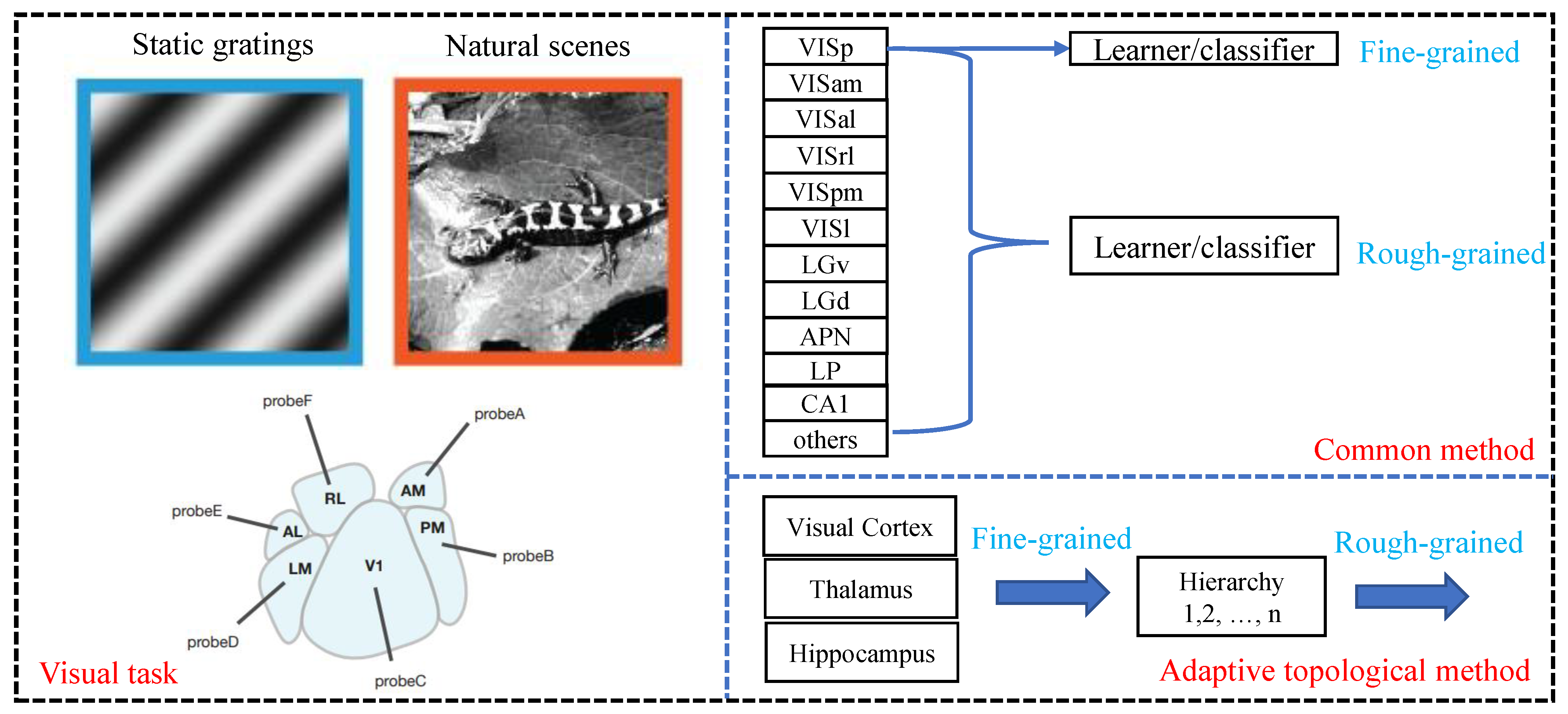
Figure 1. To understand theneural processing of visual stimuli, various visual stimuli, including natural and artificial images/videos, can be presented to animals, and the respective neural responses from primary, secondary, and higher-order visual areas can be recorded.
Mathematics 14 00031 g001
Figure 3. Compared withAT-ViT, topo-ViT can be used for ablation experiments; it can be also used to verify whether there are factors such as noise in the neural data that can be eliminated to better extract topological features. Here, the ViT consists of 6 transformer layers, each with 32 attention heads and a hidden size of 64. In the feedforward network of the Transformer, the hidden layer is set to 4.
Mathematics 14 00031 g003
Figure 4. We employed a simple SVM algorithm and applied an adaptive dimensionality reduction algorithm (ada-PCA/SVM). The bar chart shows that the adaptive dimensionality reduction has certain advantages in brain’s visual data.
Mathematics 14 00031 g004
Figure 5. The decoding output information gradient in natural scenes is presented. Among them, black represents the decoding accuracy of the visual cortex data, red represents the decoding accuracy of the thalamus/midbrain data, and cyan represents the decoding accuracy of the hippocampal data.
Mathematics 14 00031 g005
Table 1. The visual (neural) data of mice are decoded by SVM in each brain area, and the reference random accuracy (%) for natural scenes/static gratings is 0.78/16.67. Here, the random accuracy is used to evaluate the possibility of random prediction of the model, which has a significant reference value. For example, in natural scenes, the possibility of random prediction for 128 scene class-labels is R b = 1 / 128 = 0.78 % (ref); in static gratings, the possibility of random prediction for 6 direction class-labels is R b = 1 / 6 = 16.67 % (ref). Here, the bold font indicates the highest decoding accuracy in a single brain region, the gray font indicates the lowest decoding accuracy in a single brain region, and the “–” symbol indicates that there is no collected data for that single brain region in a id_session.
id (nat)VISpVISamVISalVISrlVISpmVISlLGvLGdAPNLPCA1
76141822654.6959.8563.7134.6216.4439.781.602.520.81
76367339346.6732.0316.1712.180.6266.295.112.440.79
77341890630.9410.1743.269.193.180.76
79131984751.7019.7520.9617.5012.6416.8711.732.982.070.97
79782835732.177.123.725.606.5014.673.388.070.74
79891142449.5321.6542.7716.5539.5637.450.8219.531.71
79986434250.2927.4824.6612.0831.3651.080.9414.620.76
avg45.1419.7032.5420.1117.9222.9316.5640.032.518.210.93
std8.888.8118.2218.2512.0710.6613.3623.371.536.740.32
avg-ref44.3618.9231.7619.3317.1422.1515.7839.251.737.430.15
I n f o r 1.000.430.720.440.390.500.360.880.040.170.003
76141822666.6071.7266.0059.1932.8045.5119.2920.9616.36
76367339360.8852.0243.6031.4914.8060.6725.9919.7114.83
77341890654.6936.8963.2732.7220.3116.21
79131984765.1551.9942.2359.2938.4441.7631.7218.4920.7216.82
79782835748.9836.8723.3531.1725.5931.9922.9521.5016.85
79891142465.8360.1668.7443.6158.4047.1716.6634.3320.29
79986434269.8048.0860.1656.4858.8653.5216.8337.7117.30
avg61.7047.6754.9147.5541.0744.5031.6244.5520.3425.8216.95
std6.878.4316.9712.4113.8412.1111.4715.973.317.301.54
avg-ref45.0331.0038.2430.8824.4027.8314.9527.883.679.150.28
I n f o r 1.000.690.850.690.540.620.330.620.080.200.006
Table 2. Based on the decoding results obtained in the brain’s visual system, the amount of visual information contained in each brain area is evaluated and then divided into four hierarchical structures. Here, the ✓ indicates that these single brain regions have been selected at this hierarchy, and the “–” symbol indicates that these single brain regions have not been selected at this hierarchy.
Hierarchy n, IdVISpVISamVISalVISrlVISpmVISlLGvLGdAPNLPCA1Others
n = 1
n = 2
n = 3
n = 4
760345702
762602078
Disclaimer/Publisher’s Note: The statements, opinions and data contained in all publications are solely those of the individual author(s) and contributor(s) and not of MDPI and/or the editor(s). MDPI and/or the editor(s) disclaim responsibility for any injury to people or property resulting from any ideas, methods, instructions or products referred to in the content.