Article

Vehicle Sideslip Angle Redundant Estimation Based on Multi-Source Sensor Information Fusion

by
Danhua Chen
1,2,3,
Jie Hu
1,2,*,
Guoqing Sun
1,2,
Feiyue Rong
4,
Pei Zhang
1,2,
Yuanyi Huang
3 and
Ze Cao
1,2
1
State Key Laboratory of Light Superalloys, Wuhan University of Technology, Wuhan 430070, China
2
Hubei Key Laboratory of Advanced Technology for Automotive Components, Wuhan University of Technology, Wuhan 430070, China
3
SAIC GM-Wuling Automobile Co., Ltd., Liuzhou 545007, China
4
CATARC Component Technology Co., Ltd., Tianjin 300300, China
*
Author to whom correspondence should be addressed.
Mathematics 2026, 14(1), 183; https://doi.org/10.3390/math14010183
Submission received: 2 December 2025 / Revised: 22 December 2025 / Accepted: 31 December 2025 / Published: 3 January 2026

Abstract

The sideslip angle is a key state for evaluating the lateral stability of a vehicle. Its accurate estimation is crucial for active safety and intelligent driving assistance systems. To improve the estimation accuracy and robustness of the sideslip angle for distributed drive electric vehicles (DDEV) under extreme maneuvering conditions, this paper proposes a redundant estimation scheme based on multi-source sensor information fusion. Firstly, a dynamic model of the DDEV is established, including the vehicle body dynamics model, wheel rotation dynamics model, tire model, and hub motor model. Subsequently, robust unscented particle filtering (RUPF) and backpropagation (BP) neural network algorithms are developed to estimate the sideslip angle from both the vehicle dynamics and data-driven perspectives. Based on this, a redundant estimation scheme for the sideslip angle is developed. Finally, the effectiveness of the redundant estimation scheme is validated through the Matlab/Simulink-CarSim co-simulation platform using MATLAB R2022b and CarSim 2020.0.

1. Introduction

With rapid technological advancements, the global automotive industry is accelerating its transformation towards electrification, intelligence, connectivity, and sharing. The development of smart, connected, and new energy vehicles is essential to achieving low-carbon goals and promoting sustainable development in the transportation industry. As a core technology in this transition, the automotive steer-by-wire chassis plays a critical role [1].
Distributed drive electric vehicles (DDEV) offer advantages such as precise power response and modular design flexibility, making it an ideal platform for implementing advanced driver-assistance systems in intelligent vehicles [2]. However, their inherent over-actuated nature poses a significant challenge to vehicle stability control. The sideslip angle, a crucial state for evaluating vehicle stability, can currently only be measured directly using costly sensors or estimated indirectly through algorithms. The high cost of these sensors makes them impractical for mass production, while existing estimation algorithms often lack sufficient accuracy under extreme driving conditions.
Consequently, to develop more accurate and robust control technologies for intelligent vehicles, it is necessary to fully consider the statistical uncertainties of sensor noise and the strong nonlinear dynamics of the vehicle under extreme conditions.
In the existing research on sideslip angle estimation, the estimation methods can be mainly divided into three categories: kinematic model-based methods, dynamic model-based methods, and data-driven methods [3,4,5].
Kinematic model-based methods primarily rely on the direct integration of sensor signals, typically combining data from the Global Positioning System (GPS) and Inertial Navigation System (INS). For instance, Li et al. [6] conducted an experimental comparison between the direct integration approach and other estimation techniques. Bevly et al. [7] developed a classic two-degree-of-freedom vehicle model and integrated it with GPS/INS measurements to obtain highly accurate sideslip angle estimation results. These methods are robust but are highly dependent on sensor accuracy in real-world applications. Additionally, direct integration can also lead to the accumulation of errors over time.
Dynamic model-based techniques, through the establishment of state observers, can decrease sensor reliance and are currently the predominant approach for estimating the sideslip angle. Chen et al. [8] proposed a Sliding Mode Observer (SMO) for sideslip angle estimation using the UniTire tire model, which reduced computational load and achieved accurate estimation results. Chen et al. [9] introduced a Robust Observer (RO), which achieved more accurate estimation results compared to the Leuenberger Observer (LO). Cheli et al. [10] developed a hybrid combined kinematic and dynamic observer integrated with fuzzy logic control to improve estimation accuracy.
Among dynamic model-based methods, the Kalman Filter (KF) is widely used due to its robustness against model errors, environmental noise, and real-time computation. However, since vehicles exhibit strong nonlinear behavior during motion and KF is only suitable for linear systems, several KF variants have been developed. The Unscented Kalman Filter (UKF) employs the Unscented Transformation (UT) to model the probability distribution of nonlinear functions, achieving accuracy equivalent to the second-order Taylor expansion. Wang et al. [11] proposed a UKF algorithm for sideslip angle estimation and validated its performance through joint simulations, demonstrating that UKF provides high estimation accuracy under various operating conditions. The Cubature Kalman Filter (CKF) uses a third-order spherical volume criterion for high-dimensional nonlinear estimation problem. Xin et al. [12] introduced a CKF algorithm that achieved high precision for sideslip angle estimation. However, KF-based methods and variants are only applicable when noise follows a Gaussian distribution. In practical applications, the uncertain characteristics of noise during vehicle operation can degrade the accuracy of real-time sideslip angle estimation, particularly when the noise is non-Gaussian.
Data-driven estimation methods belong to model-free methods that can alleviate the limitations of kinematic or dynamic models on estimation precision. Chindamo et al. [13] adopted a 5-10-1 three-layer Artificial Neural Network (ANN) architecture for estimating the sideslip angle of vehicles, aiming to improve the performance of active safety systems. Gao et al. [14] designed an estimation algorithm based on Hybrid Neural Networks (HNN), utilizing the vehicle dynamic characteristics to achieve accurate state estimation without relying on dynamic models. Gräber et al. [15] combined Recurrent Neural Networks (RNN) with kinematic models and proposed a supervised machine learning method for estimating the sideslip angle. Zha et al. [16] combined model-driven approaches with Radial Basis Function (RBF) neural network methods and applied weighted fusion to the estimation results. Ghosh et al. [17] introduced a deep learning (DL) method for estimating the sideslip angle in all-wheel-drive vehicles, demonstrating excellent estimation results.
Although data-driven methods effectively solve the state-estimation problem in complex nonlinear systems, the performance of such methods depends heavily on the completeness of the training data. Since training data rarely include all driving scenarios and high-quality data are hard to collect, the estimation performance will deteriorate under non-typical conditions.
To overcome these limitations, researchers have started to explore strategies that integrate data-driven methods with model-based approaches. Novi et al. [18] proposed a method that combines an ANN with a UKF, in which the ANN predicts the vehicle sideslip angle and provides it to the UKF as a pseudo-measurement. However, the ultimate accuracy of this method is still limited by the predictive performance of the ANN. Based on this, Kim et al. [19] introduced a Deep Ensemble Long Short-Term Memory (DE-LSTM) network coupled with a UKF, where the neural network outputs the predicted sideslip angle together with its uncertainty and then uses this uncertainty to adaptively tune the UKF measurement noise covariance matrix, leading to more accurate estimation results. Li et al. [20] proposed a Hybrid Physics–Data-Driven (HPDD) observer that embeds the vehicle dynamic models directly into a neural network via ridge regression and combines it with a Dual-Stage attention LSTM (DA-LSTM) to enhance spatiotemporal feature extraction, thereby achieving high-accuracy vehicle sideslip angle estimation under data-scarce conditions. Gong et al. [21] proposed a physics-guided Gated Recurrent Unit (GRU)–self-attention neural network that embeds the vehicle’s kinematic and dynamic models into the GRU to form sub-estimators and employs the Soft Actor-Critic (SAC) reinforcement learning algorithm to adaptively adjust their weights, thereby ensuring high estimation accuracy under different operating conditions.
Although existing hybrid model–data-driven methods have made progress in estimating the vehicle sideslip angle, most studies assume that all sensors always operate normally. This leads to a lack of redundancy and fault-tolerant designs for essential sensors, such as wheel speed sensors. Additionally, when developing neural network-based models, a large number of measurable signals are often used directly as inputs without systematically analyzing variable correlations and redundancies. This leads to high input dimensionality and significant information overlap, making it difficult to maintain reliable performance in cases of sensor faults or signal loss.
To address the aforementioned issues, this paper proposes a redundant estimation scheme for the vehicle sideslip angle, which employs the Robust Unscented Particle Filter (RUPF) as the main estimator and a Back Propagation Neural Network (BPNN) as the redundant estimator. Under normal sensor operation, the main estimation is provided by the RUPF based on the vehicle dynamics model. When a failure in the wheel speed sensor is detected, the system switches to the BPNN for estimation. To reduce dependence on multiple sensors and minimize input redundancy, this paper utilizes Pearson Correlation Coefficient (PCC) analysis and Random Forest (RF) feature importance assessment to filter candidate input variables, thereby constructing a BPNN redundant estimator based on a limited number of key signals.
The rest of this paper is organized as follows. Section 2 establishes a 7 Degree of Freedom (DOF) vehicle dynamics model. Section 3 presents the design of the RUPF-BPNN-based redundant estimation scheme for the vehicle sideslip angle. Section 4 validates the proposed method through simulations. Finally, Section 5 concludes the study.

2. Vehicle Dynamics Model

2.1. Vehicle Body Dynamics Model

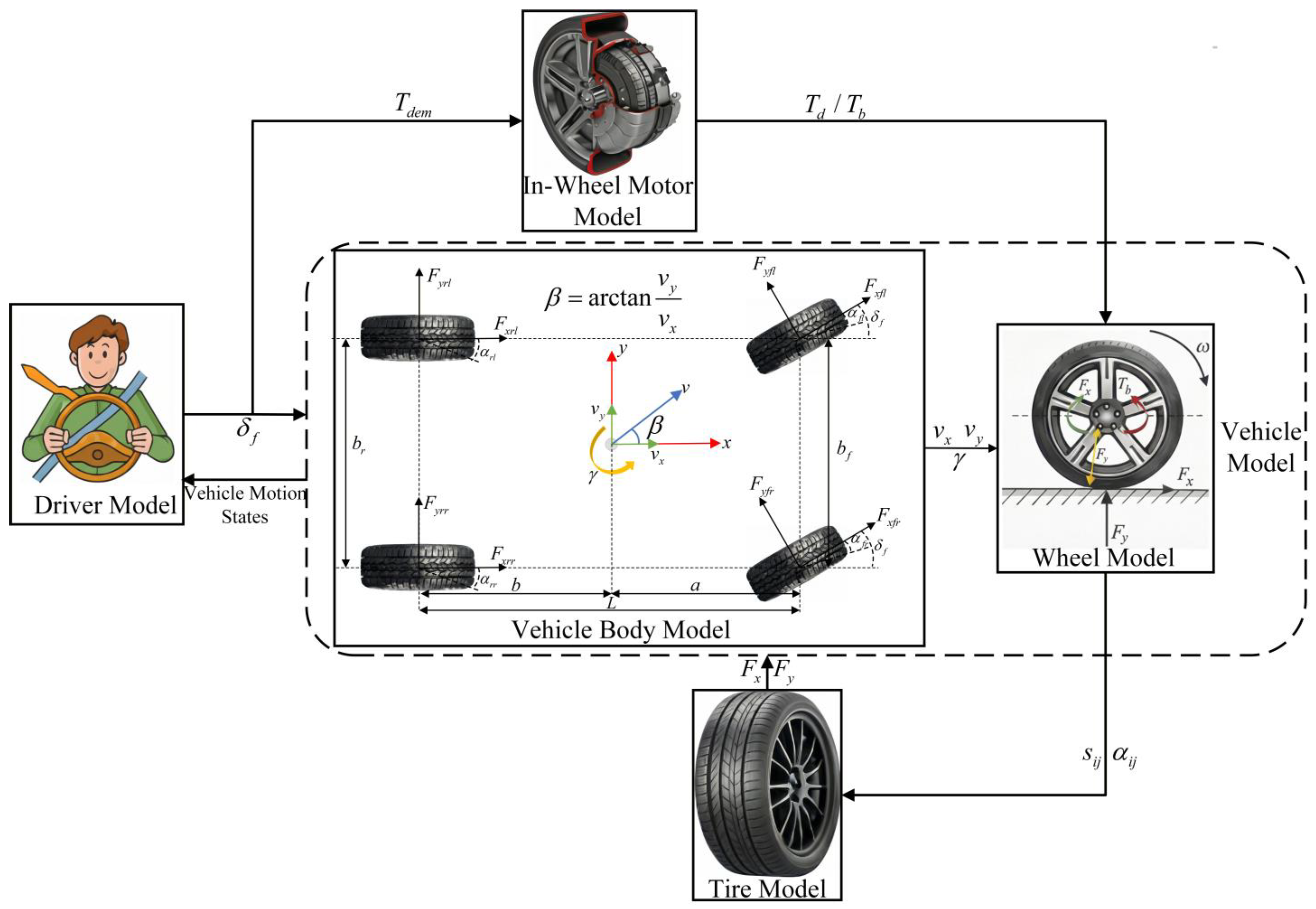
The vehicle body has 6 DOF in its coordinate system: longitudinal, lateral, vertical, roll, pitch, and yaw. Focusing on vehicle state estimation, only motion in the XY plane (longitudinal, lateral, yaw) is considered. Moreover, because the DDEV enables independent and precise control of each wheel’s speed and torque, four-wheel rotational degrees of freedom are included. This leads to the development of a 7DOF vehicle dynamics model, which includes longitudinal motion, lateral motion, yaw rotation, and the individual rotation of all four wheels, as depicted in Figure 1. This model is based on the following assumptions:
(1)
Road slope and unevenness are neglected; the road surface is assumed to be perfectly flat and horizontal, eliminating motion along the z-axis.
(2)
The effects of suspension system are ignored; vertical, roll, and pitch motions, as well as their coupling effects on other motions, are neglected.
(3)
Steering system delay is ignored, and only the front wheels steer with the same angle for both the left and right wheels.
(4)
Air resistance and tire torque effects are neglected, and all four wheels are assumed to be identical in their mechanical properties and tire dynamics.
The equations for the nonlinear 3-DOF vehicle body dynamics model are given as follows:
F x f l + F x f r cos δ f F y f l + F y f r sin δ f + F x r l + F x r r = m a x
F x f l + F x f r sin δ f + F y f l + F y f r cos δ f + F y r l + F y r r = m a y
F x f r F x f l cos δ f + F y f l F y f r sin δ f b f 2 + F x r r F x r l b r 2 + F x f l + F x f r sin δ f + F y f l + F y f r cos δ f a F y r l + F y r r b = I z γ ˙
When the vehicle steers, the tires are subjected to lateral forces, resulting in a slip angle that causes the tires to deviate from their plane of motion. This further leads to a yaw angle β between the vehicle’s actual direction of motion and the x-axis of its coordinate system. The value of β can be defined as the arctangent of the lateral velocity divided by the longitudinal velocity. Given that β remains small under typical driving conditions (|β| ≤ 5°), the arctangent function can be approximated as:
β = arctan v y v x v y v x
The longitudinal and lateral accelerations of the vehicle can be expressed as:
a x = v ˙ x v y γ a y = v ˙ y + v x γ
where a and b are the distances from the center of gravity (COG) to the front and rear axles; m is the vehicle mass; L is wheelbase; Iz is yaw inertia moment; bf and br are track width of axles; δf is on behalf of front wheel steering angle; γ is yaw rate; vx and vy are longitudinal and lateral speeds; ax and ay are longitudinal and lateral accelerations; α is slip angle of wheel; Fxij and Fyij are longitudinal force and lateral force exerted on wheels; and ij = fl, fr, rl, rr, which stands for left front, right front, left rear, and right rear wheels, respectively.

2.2. Wheel Rotational Dynamics Model

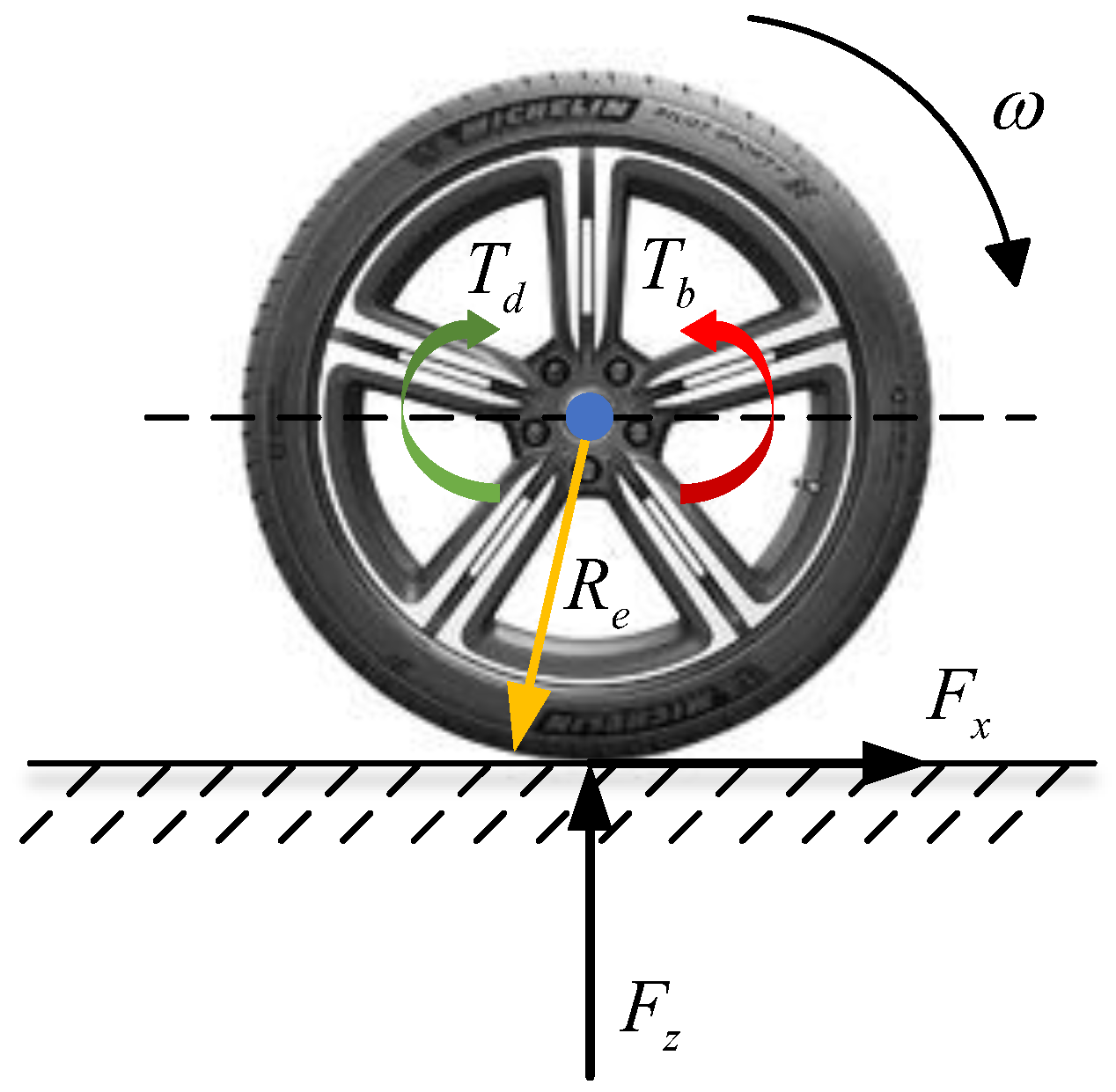
The wheel rotational dynamics model is illustrated in Figure 2. The wheel drive/braking torque is provided directly by the hub motor.
The relationship between the wheel drive/braking torque, angular acceleration, and tire rolling resistance during driving is expressed as:
J ω ˙ i j = T d T b F x i j + F f R e
Throughout the vehicle’s operation, the vertical load on each wheel varies due to steering and braking, which can be computed as follows:
F z f l = m g b 2 L m a x h g 2 L m a y b h g L b f F z f r = m g b 2 L m a x h g 2 L + m a y b h g L b f F z r l = m g a 2 L + m a x h g 2 L m a y a h g L b r F z r r = m g a 2 L + m a x h g 2 L + m a y a h g L b r
In Equation (7), the positive (+) and negative (−) signs represent the direction of dynamic load transfer caused by vehicle inertia. Specifically, the signs associated with ax indicate the longitudinal load transfer from the front to the rear axle during acceleration, while the signs associated with ay denote the lateral load transfer from the inner to the outer wheels during cornering.
The longitudinal tire slip ratios of wheels are denoted as:
s x i j = ω i j R e v x i j ω i j R e , ω i j R e v x i j ( D r i v i n g ) v x i j ω i j R e v x i j , ω i j R e < v x i j ( B r a k i n g )
where J is wheel moment of inertia; hg is the vehicle center of gravity height; Re is the effective tire radius; ωij is rotational angular velocity of wheels; Td is the driving torque; Tb is the braking torque; Ff is the rolling resistance, with Ff = f·Fz, where f is the rolling resistance coefficient; Fz is the vertical load; sx is the longitudinal slip ratio.

2.3. Tire Model

The magic formula (MF) tire model uses a combination of trigonometric functions to uniformly express the tire forces and moments. To simplify the model and reduce the computational load of controller, the Magic Formula is simplified to maintain accuracy and the coupling of longitudinal and lateral forces while lowering the computational demand. The model calculates the longitudinal and lateral tire forces in a unified form under different conditions as follows:
y M F x = D sin C arctan B X E B X arctan B X Y M F x = y M F x + S v X = x M F + S h
where YMF is the output of MF, either the longitudinal force Fx or lateral force Fy; xMF represents the tire longitudinal slip angle α or slip ratio sx; B, C, D, E denotes the curve correction factors of the MF model, which are the stiffness factor, curve shape factor, peak factor and curvature factor, respectively. Sv is the vertical offset, assumed to be 0; Sh is the horizontal offset, also assumed to be 0.
To further reflect the effect of the road adhesion on the tire forces, the longitudinal and lateral tire forces are modified based on the work of Bakker et al. [22]. The specific corrections are as follows:
F x 0 s x = μ μ 0 F x μ 0 μ s x F y 0 α = μ μ 0 F y μ 0 μ α
During vehicle operation, longitudinal and lateral slip always occur simultaneously, resulting in coupled tire forces. Therefore, to correct the lateral/longitudinal forces under pure sideslip/longitudinal slip conditions, tire forces can be solved under the equivalent combined slip ratio. The formula for calculating the forces in these combined conditions is as follows:
F x = σ x σ F x 0 s x , F y = σ y σ F y 0 α σ x = s x 1 + s x , σ y = tan α 1 + s x , σ = σ x 2 + σ y 2
where Fx and Fy denote the longitudinal and lateral tire forces under combined slip conditions. Fx0(sx) is the longitudinal tire force under pure longitudinal slip, expressed as a function of the longitudinal slip ratio sx. Fy0(α) is the lateral tire force under pure sideslip, expressed as a function of the tire sideslip angle α. σx and σy are the normalized longitudinal and lateral slip components in combined-slip conditions, and σ is the magnitude of the equivalent combined slip.

2.4. Hub Motor Model

The in-wheel motor utilized in this study is an outer-rotor permanent magnet synchronous motor from Protean Electric company. It incorporates integrated power and electronic control systems, with a peak efficiency exceeding 93%. The motor is equipped with built-in sensors for measuring speed and torque. Its internal electronic control unit enables rapid response to external torque commands. The performance specifications are listed in Table 1.
Due to the physical characteristics of the sensor, CAN communication delays, and other factors, there is a certain delay between the command signal and the actual execution by the motor, and the torque may exhibit slight oscillations. To most effectively reflect the actual response characteristics of the motor while reducing model complexity, its response characteristics are replaced with a first-order inertia element. The relationship between the actual response torque of motor and the required torque can be written as follows:
T r = 1 τ d s + 1 min T max , T d e m
where Tr is actual response torque; Tdem is the required torque; Tmax is the maximum output torque; τd is the time constant, calibrated by experiments, with a value of 0.0025 used in this study.

2.5. Driver Model

In order to track the target vehicle speed, a driver model is developed. The driver model is a longitudinal speed tracking controller in essence. Proportional-integral derivative (PID) control is adopted to make the speed error between the desired vehicle speed and actual vehicle speed close to zero, as well as to obtain the longitudinal torque required by the vehicle.
By combining the driver model with the vehicle dynamics and tire models, the comprehensive system framework is constructed. Figure 3 illustrates the 7-DOF full vehicle model architecture, depicting the signal flow among the respective subsystems.

3. The Design of the Estimator for Sideslip Angle Estimation

3.1. RUPF-Based Sideslip Angle Estimation

For the estimation of the sideslip angle, the Kalman Filter (KF) and its variants assume that noise signals follow a Gaussian distribution. This assumption significantly deviates from practical conditions, rendering it unsuitable for applications that require accurate sideslip angle estimation. Particle Filter (PF) can effectively address nonlinear non-Gaussian estimation problems. However, it still faces challenges in finding a suitable importance density function and dealing with particle degradation [23]. As the number of iterations increases, the particles with low weights decrease or vanish, leading to a drop in particle diversity. Particle degradation wastes computational resources on irrelevant particles and reduces result accuracy. To address particle degradation phenomenon, common techniques include increasing the number of particles, using resampling methods, and developing more effective importance density functions [24,25]. The key idea behind increasing the number of particles is to enhance particle diversity; however, this increases the burden on the controller, making it unsuitable for real-time vehicle control systems. Resampling methods, such as polynomial resampling and system resampling, have lower computational complexity and can effectively improve PF performance. Finally, choosing an appropriate importance density function is crucial for ensuring the effectiveness and accuracy of PF. Traditional PF algorithms use the state transition probability as the importance density function, which results in particle weight updates being only related to the previous state, failing to fully utilize the latest measurement information and thus reducing estimation accuracy.
To solve the problems mentioned above, an RUPF algorithm is proposed, which uses Particle Filter (PF) as the main framework. The algorithm uses the Unscented Kalman Filter (UKF) to predict the importance density function and adjusts it using real-time observations. Additionally, resampling techniques are applied to reduce particle degradation, thereby improving both the accuracy and robustness of the estimation results. It should also be noted that comparisons between the RUPF method and EKF, UKF, and standard PF have been conducted in previous work by the authors [26]. The results demonstrate that the RUPF method achieves superior estimation performance under non-Gaussian noise conditions compared to conventional filtering approaches. Thus, the RUPF method is applied directly in this work.
The discretized form of the nonlinear system is expressed as below:
x k + 1 = f x k , u k + w k z k = h x k , u k + v k
where f (·) and h (·) are the system prediction and measurement functions; x is the state variable; z is the measurement variable; u is the input variable; w and v represent the process noise and measurement noise, which are non-Gaussian. The subscripts k and k + 1 indicate discrete time steps.
The procedure for the RUPF algorithm involves the following steps:
(1)
Initialization: sample N particles { x 0 i } i = 1 N with same weights 1/N generated by the prior PDF p(x0):
x ^ 0 i = E x 0 i , P 0 i = E x 0 i x ^ 0 i x 0 i x ^ 0 i T
(2)
Calculate the importance density using UKF:
Construct Sigma points based on symmetric sampling strategy:
χ ( 0 ) i = x ^ 0 i , l = 0 χ ( l ) i = x ^ 0 i + n + λ P 0 i l , l = 1 , 2 , , n χ ( l ) i = x ^ 0 i n + λ P 0 i l , l = n + 1 , , 2 n
Calculate the sigma point weights:
ω ( 0 ) i m = λ n + λ , l = 0 ω ( 0 ) i c = λ n + λ + 1 α U 2 + β U , l = 0 ω ( l ) i m = ω ( l ) i c = 1 2 n + λ , l = 1 , 2 , , 2 n
where x ^ 0 i and P 0 i are the initial state and error covariance matrix, respectively; m denotes the weight of the states, and the superscript c represents the weight of P 0 i ; λ is the scaling factor, defined as λ = α u 2 n + κ n ; α u controls the range of Sigma point distribution, typically between 10−4 and 1, and is set to 0.001 in this study; κ is the second-order scaling parameter, κ = 0 when n > 3, κ = 3 − n when n ≤ 3; β u is the weight factor, with a value of 2 being optimal for Gaussian distribution.
The UT is utilized to generate the sigma points set:
χ k 1 i = x ^ k 1 i x ^ k 1 i + n + λ P k 1 i x ^ k 1 i n + λ P k 1 i
Compute the one-step prediction of the sigma points and error covariance matrix:
χ k i = f χ k 1 i , u k 1 x ^ k i = j = 0 2 n ω i m χ k i P k i = j = 0 2 n ω i c χ k i x ^ k i χ k i x ^ k i T + Q
Based on the one-step prediction, a new series of points is generated by the UT:
χ k i = x ^ k i x ^ k i + n + λ P k i x ^ k i n + λ P k i
Calculate the predicted observation values of the Sigma point set, and compute the observation mean and error covariance:
Z k i = h χ k i , u k 1 z ^ k i = j = 0 2 n ω i m Z k i P z z = j = 0 2 n ω i c Z k i z ^ k i Z k i z ^ k i T + R
Calculate the Kalman gain, and update the state and error covariance:
P x z = j = 0 2 n ω i c χ k i x ^ k i Z k i z ^ k i T K k = P x z P z z 1 x ^ k i = x ^ k i + K k z k z ^ k i P k i = P k i K k P z z K k T
(3)
Importance sampling, sampling particles:
x ˜ k i ~ q x k i x k 1 i , z k = N x ^ k i , P k i
where N(·) is a Gaussian function.
(4)
Update particle weights and normalize:
ω k i ω k 1 i p z k x ˜ k i p x ˜ k i x k 1 i q x ˜ k i x k 1 i , z k
ω ˜ k i = ω k i / i = 0 N ω k i
(5)
Systematic random resampling:
Initialization of the cumulative distribution function (CDF): c0 = 0;
Assign the CDF;
c i = c i 1 + ω ˜ k i
For N particles, generate random numbers separately:
a ~ U 0 , 1
Find the integer j that satisfies the following equation, where j = 1, 2, …, N:
c j 1 < a < c j
Copy the j-th particle once and assign it to the new particle; the particle weights are reset to 1/N, and a total of N new particles are generated after the resampling;
(6)
State the estimation output at the moment k.
x ^ k = i = 0 N ω ˜ k i x ˜ k i
Using the 7-DOF vehicle model, the RUPF algorithm is applied to estimate the vehicle sideslip angle. The state variables are defined as follows:
x β = v x , v y , γ , w f l , w f r , w r l , w r r T = x 1 , x 2 , x 3 , x 4 , x 5 , x 6 , x 7 T
The input variable is defined as:
u β = δ f
The measurement vector is defined as:
z β = a x , a y , γ , w f l , w f r , w r l , w r r T = z 1 , z 2 , z 3 , z 4 , z 5 , z 6 , z 7 T
Based on the above definitions of the state, input, and measurement vectors, the corresponding state and measurement equations can be directly derived from the 7-DOF vehicle model.

3.2. Neural Network Algorithm

3.2.1. Dataset Acquisition

Deep learning methods for estimating the sideslip angle essentially involve mapping and approximating a nonlinear function. By training on a limited dataset, the model can be generalized to predict unknown samples, allowing for the estimation of the sideslip angle under different conditions. The first step in using this method is to define suitable inputs and outputs, where the output is the sideslip angle, and the inputs require some functional mapping analysis.
The mapping relationship between the sideslip angle and all fundamental variables is established through a thorough analysis of the parameter interactions within the integrated vehicle dynamics model:
β = f a x , a y , v x , v y , γ , δ f , ω i j , T d i j , μ
Among these fundamental variables, vy and μ are not measurable using vehicle-mounted sensors. However, the front-wheel steering angle δf can be indirectly derived from the steering wheel angle δSW. Consequently, for subsequent dataset development, the functional relationship between the sideslip angle and the other fundamental variables is revised to:
β = f a x , a y , v x , γ , δ S W , ω i j , T d i j
Once the functional mapping relationship is determined, the training dataset for the neural network can be established. To accurately characterize the highly nonlinear vehicle dynamics, the data must cover vehicle responses under a wide range of operating conditions, including low and high speeds as well as low, medium, and high adhesion road surfaces. In this study, all data used for training, validation, and testing of the BP neural network are generated on a MATLAB/Simulink-CarSim co-simulation platform, instead of real-vehicle experiments, in order to avoid the high cost and safety risk associated with extreme driving conditions.
The dataset consists of standard double-lane-change (DLC) maneuvers and additional slalom maneuvers, which are designed in accordance with ISO 15037-1:2019 and ISO 3888-1:2018 [27,28]. For each maneuver, simulations are conducted at vehicle speeds from 20 km/h to 130 km/h with a 10 km/h interval. To represent different road friction conditions, the adhesion coefficient μ is set to 0.30, 0.50, and 0.85, corresponding to low, medium, and high adhesion roads, respectively. Under these combinations of maneuvers, speeds and road surfaces, the vehicle can successfully complete all tests, resulting in 37 simulation runs in total. The sensor sampling frequency is 100 Hz. The data collected includes ax, ay, vx, γ, δSW, ωij, Tdij, β as a group, with 37 datasets and 78637 rows. This dataset adequately reflects the vehicle’s dynamic response under both standard and extreme scenarios.
The vehicle can complete the tests in all speeds and road surface conditions. The specific data collection scenarios are shown in Table 2.

3.2.2. RF Feature Importance Analysis

Random Forest (RF) combines several decision trees to improve regression accuracy and can also be used for feature importance evaluation. Thus, RF is applied to analyze the relationship between the fundamental variables and the sideslip angle. In the RF algorithm, Mean Squared Error (MSE) is used as the impurity function for nodes, and the impurity for a node is calculated as follows:
G m X , V = 1 N F y l X l e f t y l y ¯ l e f t 2 + y r X r i g h t y r y ¯ r i g h t 2
The importance score of a given feature can be calculated as follows:
n m = w m G m w l e f t G l e f t w r i g h t G r i g h t
f X i = i = 1 I n i / m = 1 M n m
f X i n o r = f X i / i = 1 K f X i
where NF is the number of training samples; X is a feature in the sample; V is the split value of feature X; Xleft and Xright are the sample sets for the left and right child nodes of node m, respectively; t represents the left and right child nodes of node m; yl and yr are the values of the left and right child nodes of m; y ¯ l e f t and y ¯ r i g h t the average target values for the left and right child nodes of m; Gm(X,V) is the impurity of node m based on feature X; wm, wleft, and wright represent the proportion of samples in node m and its child nodes relative to the total samples; Gm, Gleft and Gright are the impurities of node m and its child nodes; nm is the importance of node m; M is the total number of nodes in the decision tree; ni indicates the presence of feature Xi at a node; I is the number of nodes that have feature Xi; f(Xi) indicates the importance of feature Xi; K is the total number of features in the sample; f(Xi)nor represents the normalized importance score of feature Xi.
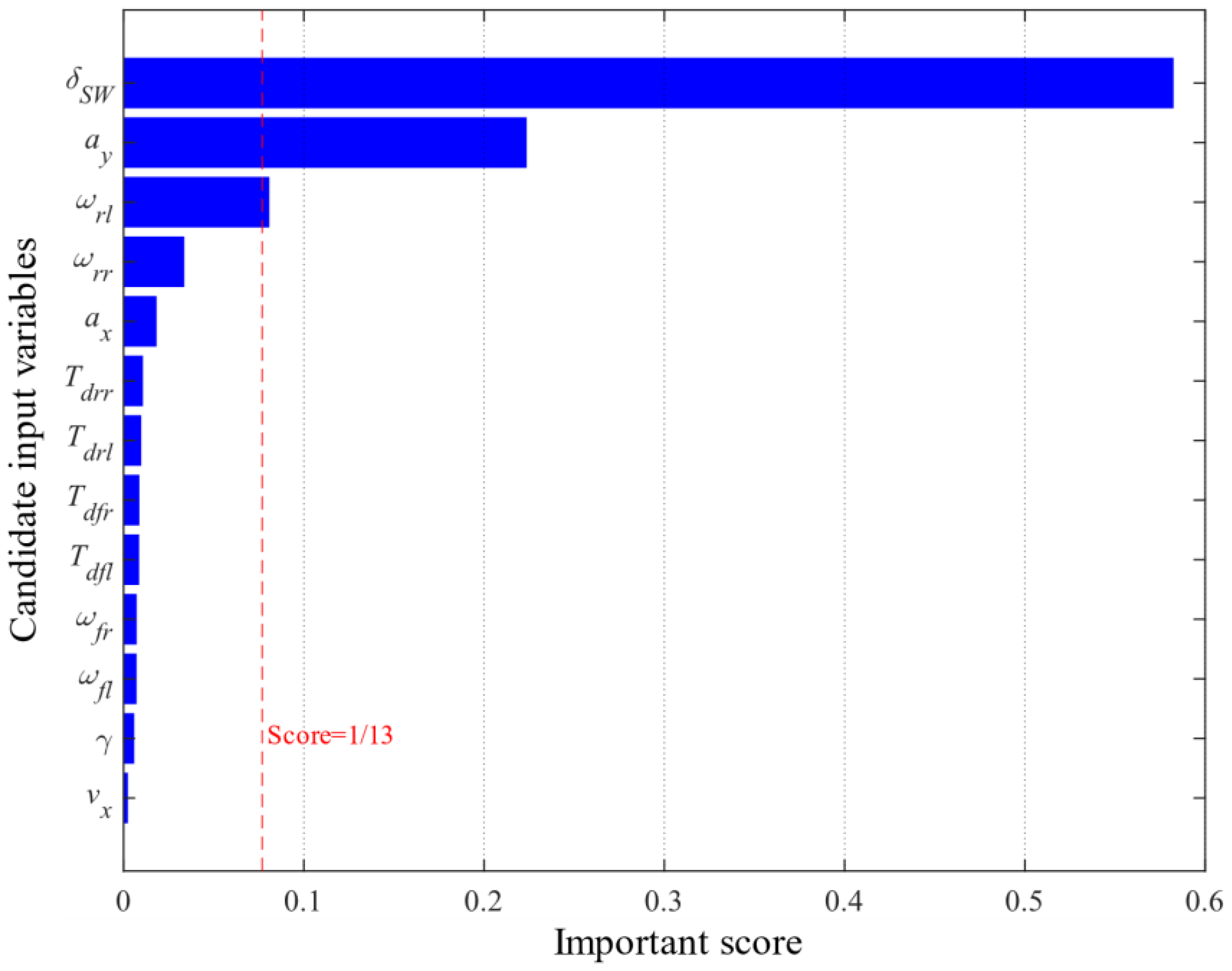
The RF feature importance analysis is performed on the dataset, with the final normalized importance score of 1/K set as the threshold standard. The results are shown in Figure 4. It is evident that the feature δSW contributes far more than other features, with ay and ωrl also exceeding the threshold. Based on the results from the PCC analysis, the input features for the subsequent deep learning algorithm can be determined to include δSW, ay, and any one of the Wheel rotational speeds ωij.
The BPNN is a typical training algorithm in deep learning, known for its excellent nonlinear mapping capabilities. The BPNN consists of three layers: input, hidden, and output layers. The input layer contains 3 neurons, with the input information being δSW, ay, and ωrl. The output layer contains 1 neuron, and the output information is β.
The number of neurons nh in the hidden layer is determined by the following equation:
n h = n i + n o + σ n
where ni and no represent the number of neurons in the input, and output layers, respectively; σn is a configurable parameter, typically an integer between 1 and 10.
In this study, ni = 3 and no = 1. The parameter σn is tuned in the range 1–10 according to the validation performance, and σn = 10 provides the best performance without obvious overfitting. Therefore, the number of neurons in the hidden layer is set to nh = 12.
Before training the neural network, the raw data are preprocessed as follows. First, for the CarSim simulations of the DLC and Slalom maneuvers, the steady-state segments before and after each maneuver are removed, and all signals are resampled and synchronized at 100 Hz. Because the CarSim simulation data are free of measurement noise, no additional filtering is applied in this study. For real-vehicle data, however, a low-pass filter should be used to suppress high-frequency measurement noise. Next, the input variables are normalized using the statistics of the entire dataset so that each variable has zero mean and unit variance. Finally, all 78,637 samples are randomly shuffled and split into training, validation, and test sets in a 70%:15%:15% ratio.
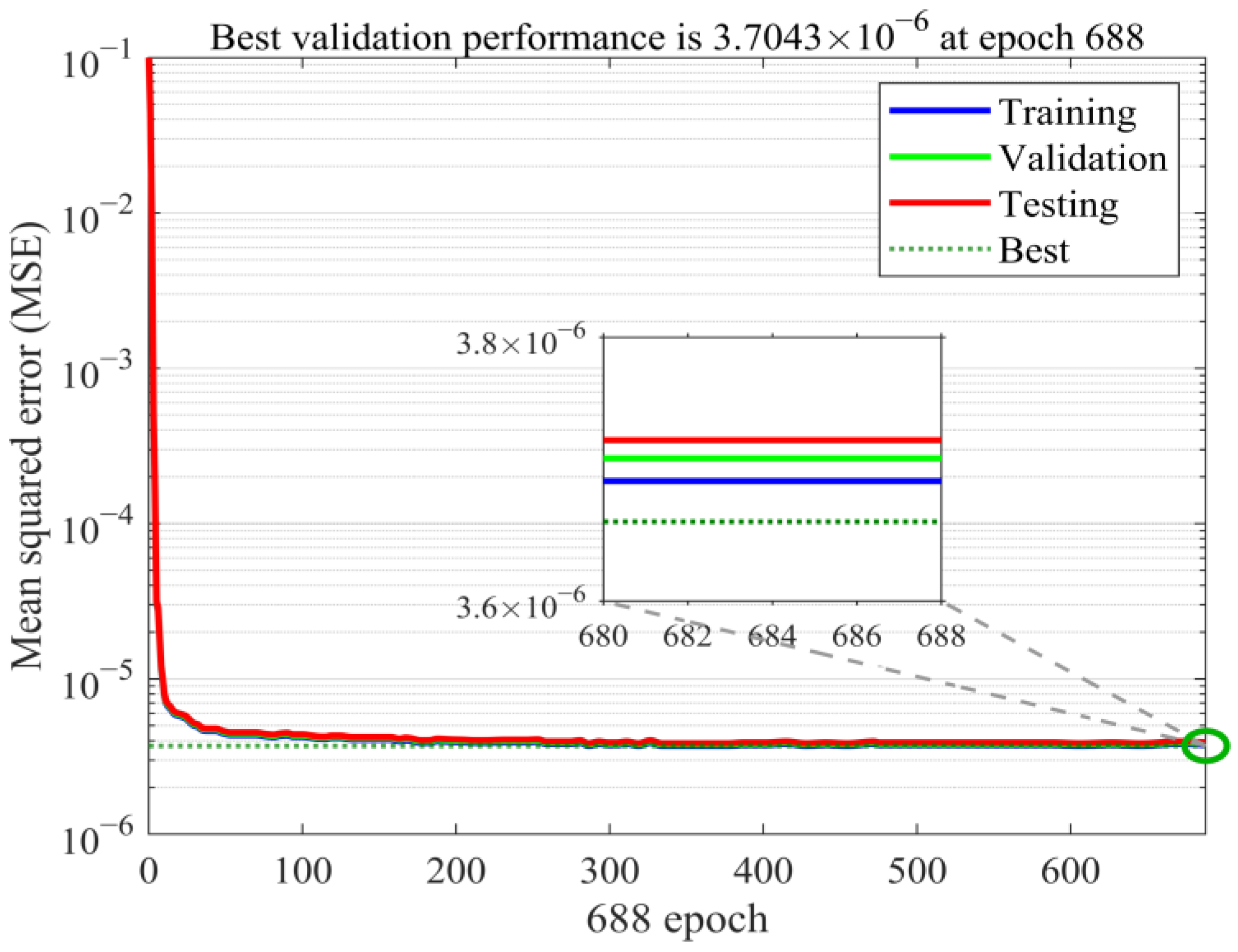
The network weights are optimized using the Levenberg–Marquardt (LM) algorithm, a second-order method that combines gradient-descent and Gauss-Newton updates. For small and medium-scale feedforward networks, LM typically achieves much faster convergence and better numerical stability than standard gradient-descent BP. Additionally, a mean squared error (MSE) is adopted as the training performance index.
Figure 5 depicts the variation in the MSE with training epoch for the BPNN. The blue, green, and red curves correspond to the training, validation, and testing datasets, respectively. The horizontal gray dotted line (“Best’’) denotes the minimum validation MSE of 3.7043 × 10⁻⁶, achieved at epoch 688. The training curve reflects how well the network fits the data used to update its parameters, the validation curve is used to monitor overfitting and to select the model (early stopping), and the testing curve provides an unbiased assessment of the final model’s generalization performance on unused samples. Figure 5 clearly shows that the training, validation, and testing curves almost coincide near convergence and lie close to the ‘Best’ line. This suggests that the final network provides accurate predictions for both the training data and the independent validation/testing data, with minimal overfitting.

3.3. Redundant Estimation Scheme Design

3.3.1. PCC Analysis

The Pearson correlation coefficient (PCC) is used to evaluate the strength of linear relationships between variables. The procedure is outlined as follows:
(1)
Correlation assessment: Calculate the correlation coefficient between each pair of variables:
R = i = 1 N P X i X ¯ Y i Y ¯ i = 1 N P X i X ¯ 2 i = 1 N P Y i Y ¯ 2
where NP represents the number of samples; X and Y are two variables; X ¯ and Y ¯ are their means.
If the correlation coefficient |R| ≥ 0.8, it indicates a very strong correlation between X and Y, allowing X to be linearly represented by Y. When |R| = 1, X and Y are fully correlated, demonstrating fault tolerance between the variables.
(2)
Significance judgment involves calculating the t-statistic between each pair of variables and then determining the significance p-value by consulting the t-distribution table. The t-statistic calculation equation is as follows:
t P = R N P 2 1 R 2
When p ≤ 0.05, it indicates a high level of significance between the two variables; when p > 0.05, the significance level is insufficient, and a large correlation coefficient R may be due to random factors.
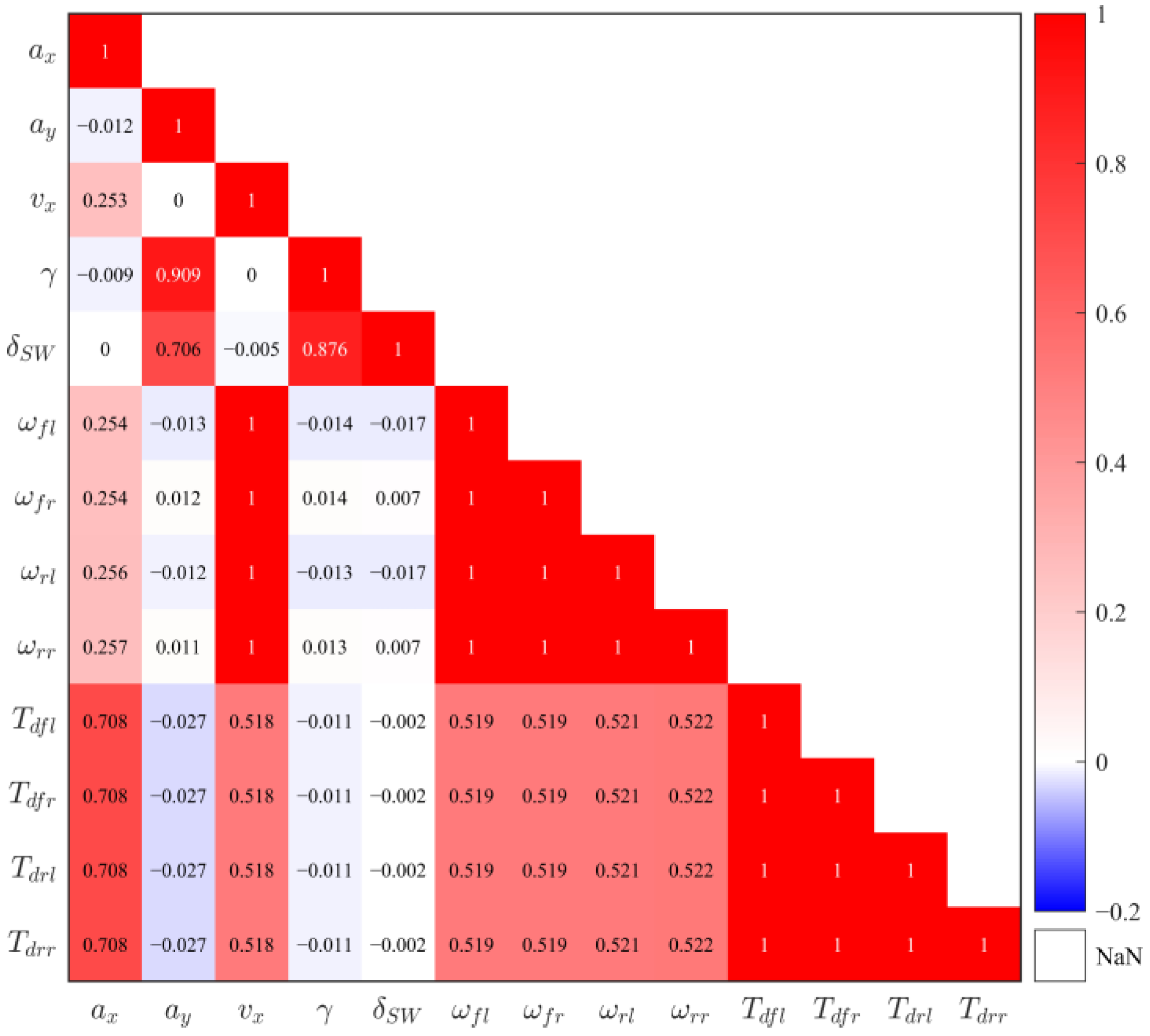
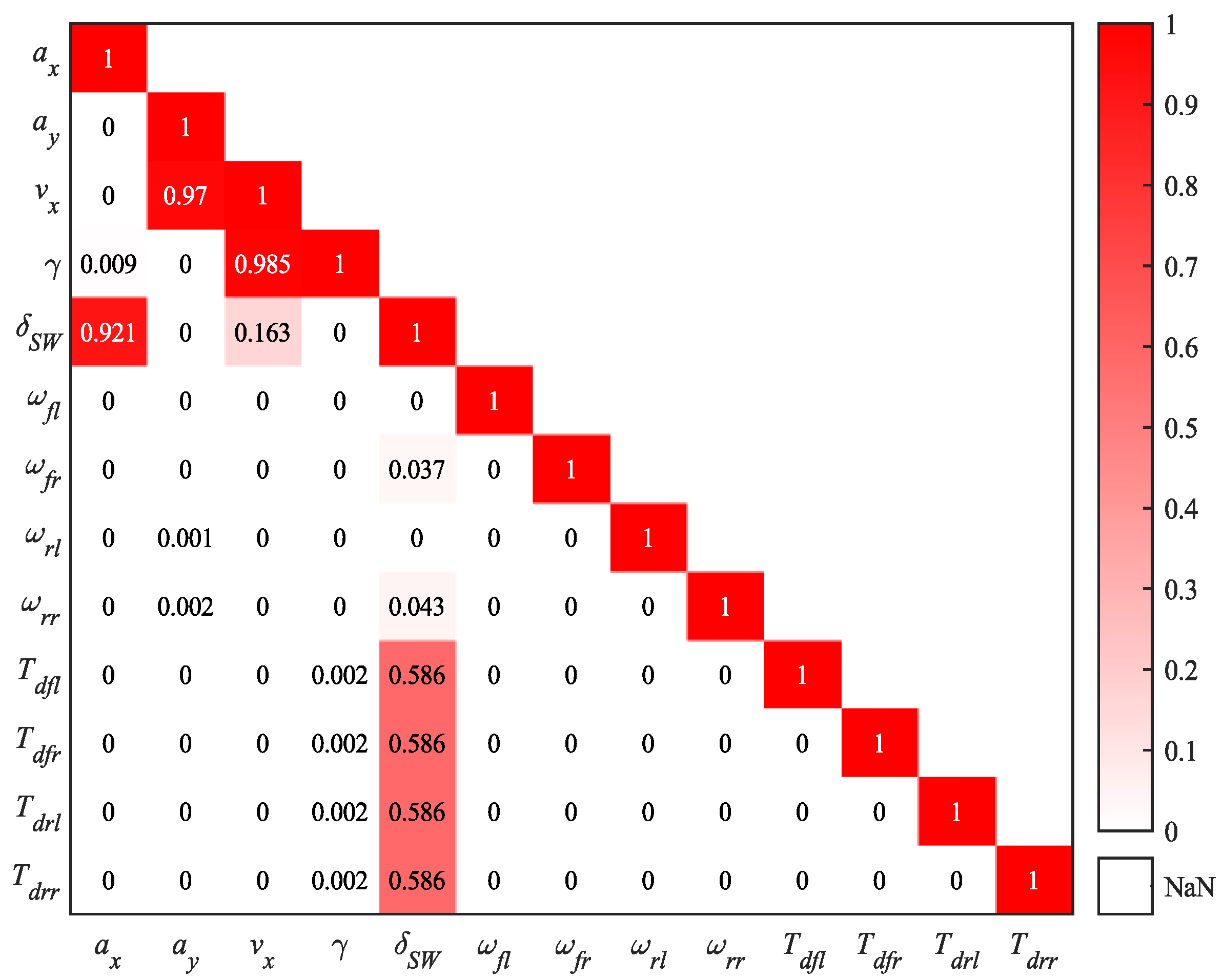
PCC analysis is performed on the collected dataset, and the resulting correlation coefficients (R-values) and significance levels (p-values) are shown in Figure 6 and Figure 7. Figure 6 illustrates the correlation among the candidate input variables. A high correlation indicates that one variable can be (approximately) represented as a linear function of another, providing the theoretical basis for the redundant design. Figure 7 further tests the significance of these correlations to determine whether the observed linear relationships are statistically meaningful or merely due to random factors. As shown in Figure 6, there is a very strong correlation between ay and γ, and between γ and δSW, while vx, ωij, and Tdij are perfectly correlated. Figure 7 illustrates that these results are not due to random factors. The perfect correlation between variables supports system redundancy. For instance, if the vx signal fails, it can be replaced by a linear transformation of ωij. Similarly, if a wheel speed signal ωij fails, it can be replaced by another wheel speed signal, and the same redundancy principle can also apply to the hub motor torque signal Tdij.

3.3.2. Redundant Estimation Scheme

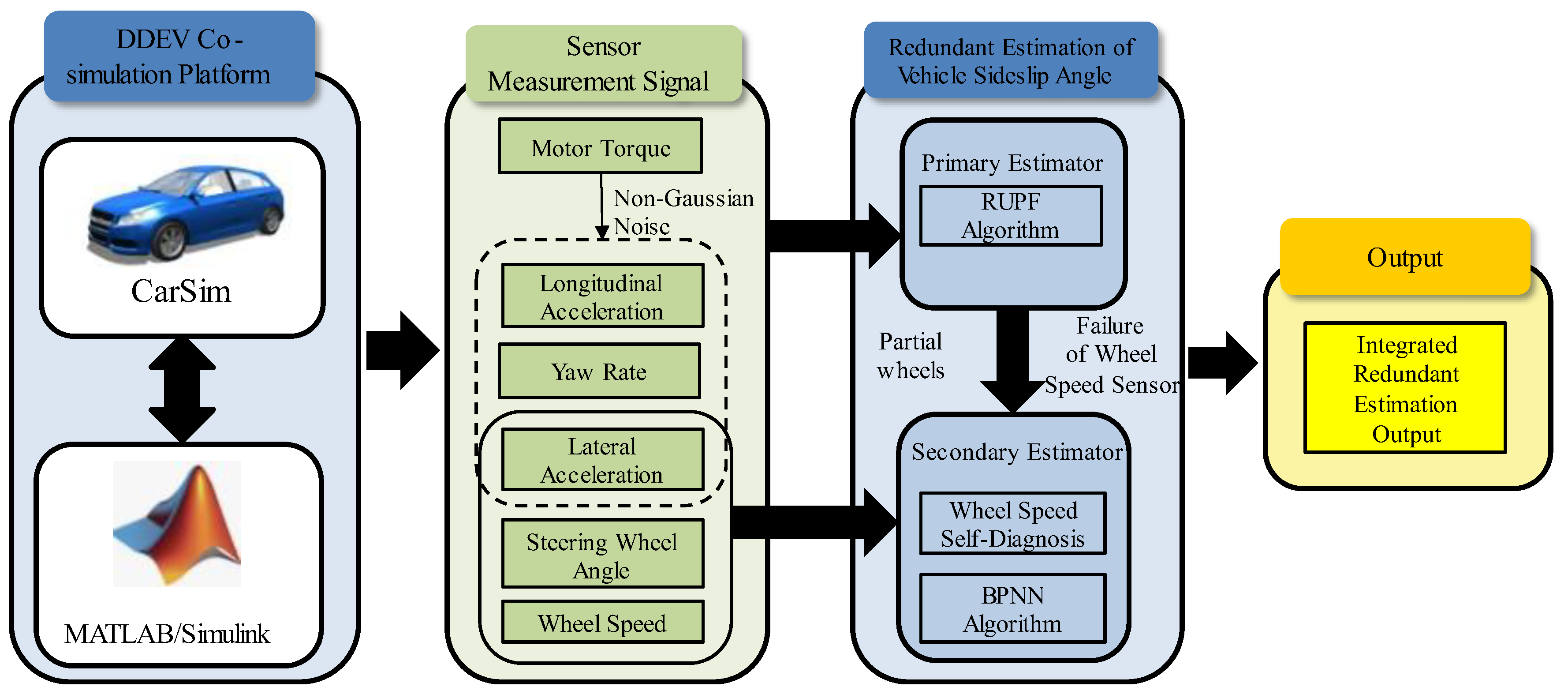
Redundancy design has become critical for intelligent vehicle control systems. When a system fails, the ability of another system to quickly compensate can help prevent accidents. Vehicle redundancy can be achieved through either hardware or software methods. Hardware redundancy relies on multiple hardware components, which is costly for mass production. In contrast, software redundancy uses redundant algorithms to enhance system stability, offering a more cost-effective and straightforward implementation. This paper adopts a software redundancy method by integrating two sideslip angle estimation algorithms to create a redundant estimation scheme, as illustrated in Figure 8.
From the data-driven sideslip angle estimation method described above, it can be found that the BPNN method can achieve redundancy by simply utilizing the wheel rotational angular velocity ωij. However, since this method directly uses the sensor signals as input, omitting a signal filtering step like that included in the RUPF algorithm, the estimation accuracy of the BPNN method is consequently lower than that of the RUPF method. Additionally, to estimate the sideslip angle using the RUPF approach, the rotational angular velocities ωij from all four wheels are required as inputs. If any of the wheel speed sensors fail, the method fails as well, providing no redundancy.
To ensure the reliable estimation of the vehicle sideslip angle, the RUPF method is used as the main estimator, while the BPNN method acts as the secondary estimator. Thus, in the redundant estimation scheme for the sideslip angle in Figure 8, the main estimator is used when the vehicle operates normally. If the rotational angular velocity signal ωij from any wheel fails, the secondary estimator is immediately activated, using the rotational angular velocity signal from any one of the functional wheels. In the case where the rotational angular velocities of all four wheels fail, the secondary estimator will also cease operation.

4. Simulation Verification

To verify the feasibility and reliability of the proposed sideslip angle redundant estimation scheme, the international standards ISO 15037-1:2019 and ISO 3888-1:2018 [27,28] are referenced. Two driving scenarios, the double-lane change (DLC) and slalom, are selected. Each maneuver is tested under varied dynamic conditions: at constant vehicle speeds of 36 km/h and 72 km/h, and on road surfaces characterized by adhesion coefficients of 0.4 (low-friction) and 0.7 (high-friction), intentionally distinct from the training dataset conditions outlined in Section 3.2.1. Furthermore, to realistically simulate sensor noise, all measurement signals are superimposed with additive Gaussian white noise, with its magnitude set to approximately 3% of the nominal signal variance. Additionally, since sensor failure detection and signal switching are completed quickly, usually within tens of milliseconds, it is assumed that there is no delay in signal switching. The essential vehicle parameters employed in the simulation are detailed in Table 3.
To quantify the estimation results, three evaluation metrics are used: Mean Absolute Error (MAE), Maximum Absolute Error (MaxAE), and Root Mean Square Error (RMSE). MAE represents the average size of the estimation errors, MaxAE is used to assess the maximum deviation, and RMSE evaluates the accuracy and robustness of the estimation results. The equations for the three-performance metrics are as follows:
M A E = i = 1 N y C i y ^ e i / N
M a x A E = max y C i y ^ e i
R M S E = i = 1 N y C i y ^ e i 2 / N
where yei represents the estimation result of the algorithm; yCi is the reference value, provided by the CarSim 2020.0 software.
In the RUPF filter, both the process noise matrix Q and the measurement noise matrix R are adjustable parameters. The process noise matrix R, which reflects the accuracy of the vehicle dynamic model, is generally difficult to obtain directly and must be determined through tuning. For this study, it is set to 10−6I7×7, where I7×7 denotes a 7 × 7 identity matrix. The measurement noise matrix R is determined by the characteristics of the sensor used and is assigned a value of 10−5I7×7 based on the actual sensor accuracy.

4.1. DLC Tests

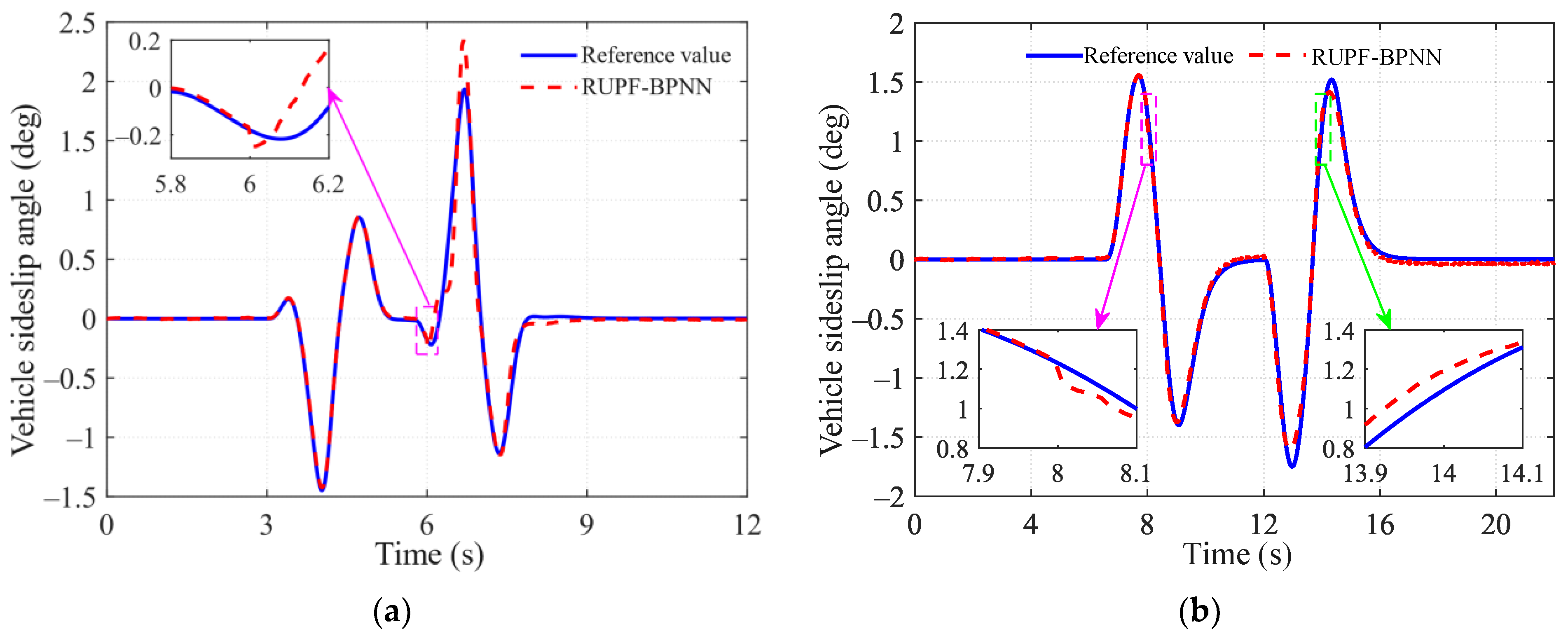
The results of sideslip β redundancy estimation in the DLC scenario are depicted in Figure 9. In Figure 9a, the primary estimator, RUPF, functions correctly until t = 6 s. At this moment, a failure in the left front wheel speed sensor causes the main estimator to become ineffective. The secondary estimator BPNN then takes over, switching to the normal right front wheel speed signal. As shown in Figure 9a, even after the failure of the main estimator, the secondary estimator continues to accurately estimate the sideslip angle, with a smooth transition between the two estimators. The maximum error is about 0.5° at t = 6.7 s. Figure 9b shows that when the left front, right front, and left rear wheel speed sensors fail at t = 8 s, t = 11 s, and t = 14 s, respectively, the redundancy estimation method still successfully identifies the sideslip angle, closely following the reference value while ensuring minimal error.
The evaluation metrics for the sideslip angle redundancy estimation results under the DLC condition are summarized in Table 4. It can be observed that the maximum absolute error of the estimation results is within 0.53°, the mean absolute error is less than 0.04°, and the RMSE is below 0.09°. This indicates that the proposed redundancy estimation scheme for the sideslip angle has high estimation accuracy under both high and low adhesion DLC conditions.

4.2. Slalom Tests

To further show the superiority of the proposed algorithm, a simulation validation of the sideslip angle redundancy estimation is conducted under the Slalom condition.
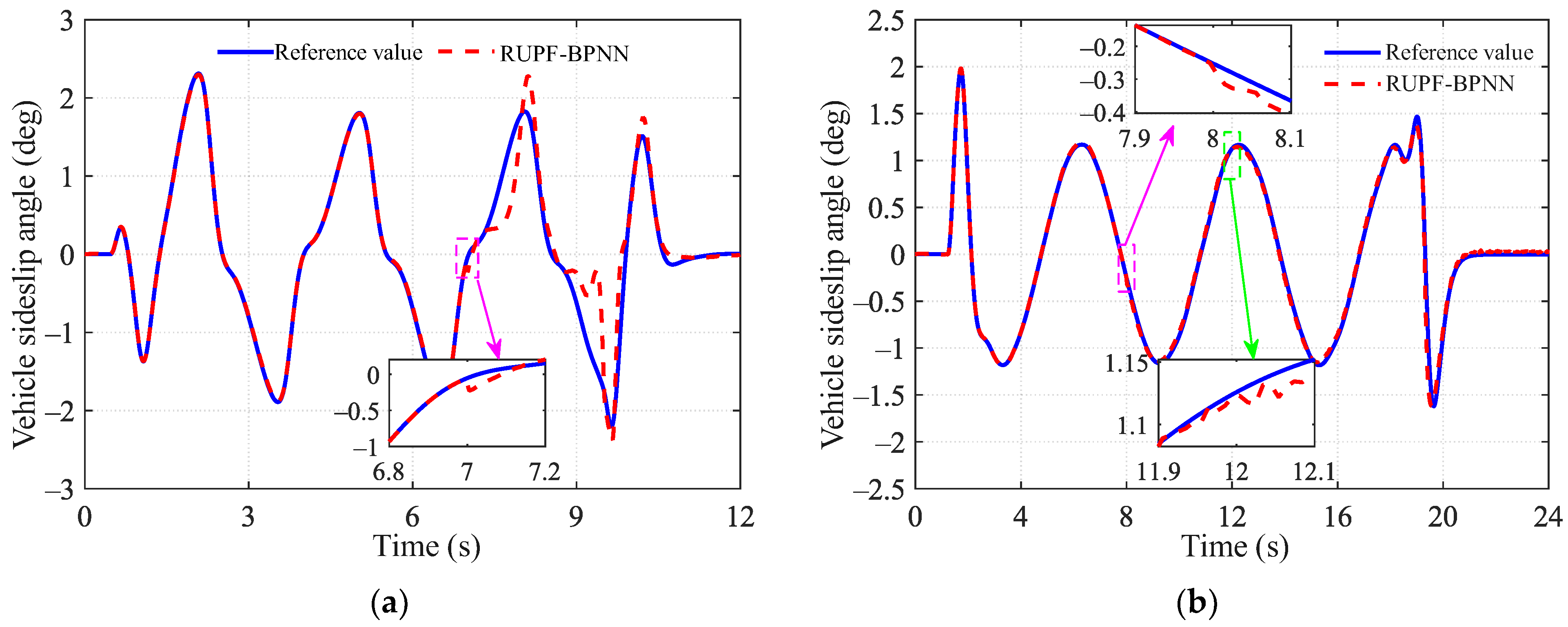
Figure 10 illustrates the redundancy estimation results of β in the Slalom scenario. In Figure 10a, at t = 7 s, the wheel speeds of the left front, right front, and left rear wheels fail simultaneously. As a result, the backup estimator, BPNN, switches to using wheel angle, lateral acceleration, and right rear wheel speed as input signals. As shown in Figure 10, the estimated results still closely follow the trend of the reference values.
The evaluation metrics for the redundancy estimation of the sideslip angle under the Slalom condition are presented in Table 5. As indicated in Table 5, the estimation result for MaxAE is within 1.3°, the MAE is under 0.11°, and the RMSE is below 0.25°. In comparison with the DLC condition, it can be observed that the vehicle in the Slalom scenario exhibits higher nonlinearity, leading to slightly higher estimation metrics. However, the error remains relatively small, suggesting that the proposed redundancy estimation scheme for the sideslip angle is still capable of producing accurate results, even when some sensors fail.

5. Conclusions

This paper proposes a redundancy estimation scheme for the vehicle sideslip angle, in which the RUPF serves as the primary estimator and a BPNN is employed as the backup estimator. The RUPF is applied when all wheel-speed sensors function properly, and the estimator is switched to the BPNN once a wheel-speed sensor fault is detected.
In the DLC scenario, the RUPF functions as the main estimator and is seamlessly replaced by the BPNN when wheel-speed sensor failures occur. The transition between the two estimators is smooth, and the estimated sideslip angle closely tracks the reference value, yielding a MaxAE within 0.53°, MAE below 0.04°, and RMSE below 0.09°. In the more challenging Slalom scenario, even with simultaneous failures of three wheel-speed sensors, the BPNN effectively utilizes the steering angle, lateral acceleration, and the remaining wheel-speed signal. As a result, the estimation errors remain within acceptable levels, with a MaxAE within 1.3°, an MAE under 0.11°, and an RMSE below 0.25°. Overall, these results demonstrate that the proposed RUPF–BPNN redundant estimation method maintains high accuracy and strong fault tolerance, even under multiple sensor failures.
In the future, Hardware-in-the Loop (HIL) simulations and real-world tests will be carried out to validate the performance of the proposed redundant estimation method. Additionally, the integration of the proposed estimator with control strategies will be explored to enhance the overall performance of the vehicle system.

Author Contributions

D.C.: Methodology, writing—review and editing, writing—original draft. J.H.: Writing—review and editing, funding acquisition, software. G.S.: Writing—review and editing, writing—original draft. F.R.: Writing—review and editing, software. P.Z.: Writing—review and editing, supervision, resources. Y.H.: Writing—review and editing, supervision, resources. Z.C.: Writing—review and editing. All authors have read and agreed to the published version of the manuscript.

Funding

This study was supported by the Technology Innovation Program of Hubei Province (2024BAB077), Guangxi Science and Technology Major Program (AA23062056), the Fundamental Research Funds for the Central Universities (WUT: 104972024KFYjc0001), Guangxi Special Hired Expert Program.

Data Availability Statement

The raw data supporting the conclusions of this article will be made available by the authors on request.

Conflicts of Interest

Danhua Chen is affiliated with SAIC GM-Wuling Automobile Co., Ltd., Liuzhou, China. Feiyue Rong is affiliated with CATARC Component Technology Co., Ltd., Tianjin, China. The authors declare that these affiliations do not influence the results or interpretation of this study, and no conflict of interest exists regarding the publication of this manuscript.

References

  1. Farrell, J.A.; Roysdon, P.F. Advanced Vehicle State Estimation: A Tutorial and Comparative Study. IFAC-PapersOnLine 2017, 50, 15971–15976. [Google Scholar] [CrossRef]
  2. Zhao, M.; Guo, H.; Zhang, L.; Liu, X. Driving Stability Control of Four-Wheel Independent Steering Distributed Drive Electric Vehicle with Single Wheel Steering Failure. J. Mech. Eng. 2024, 60, 507–522. [Google Scholar]
  3. Liu, J.; Wang, Z.; Zhang, L.; Walker, P. Sideslip Angle Estimation of Ground Vehicles: A Comparative Study. IET Control Theory Appl. 2020, 14, 3490–3505. [Google Scholar] [CrossRef]
  4. Chindamo, D.; Lenzo, B.; Gadola, M. On the Vehicle Sideslip Angle Estimation: A Literature Review of Methods, Models, and Innovations. Appl. Sci. 2018, 8, 355. [Google Scholar] [CrossRef]
  5. Huang, F.; Gao, Y.; Fu, C.; Gostar, A.K.; Hoseinnezhad, R.; Hu, M. Vehicle State Estimation Based on Adaptive State Transition Model. In Proceedings of the 2020 4th CAA International Conference on Vehicular Control and Intelligence (CVCI), Hangzhou, China, 18–20 December 2020. [Google Scholar]
  6. Li, L.; Jia, G.; Ran, X.; Song, J.; Wu, K. A Variable Structure Extended Kalman Filter for Vehicle Sideslip Angle Estimation on a Low Friction Road. Veh. Syst. Dyn. 2014, 52, 280–308. [Google Scholar] [CrossRef]
  7. Bevly, D.; Ryu, J.; Gerdes, J. Integrating INS Sensors with GPS Measurements for Continuous Estimation of Vehicle Sideslip, Roll, and Tire Cornering Stiffness. IEEE Trans. Intell. Transp. Syst. 2006, 7, 483–493. [Google Scholar] [CrossRef]
  8. Chen, Y.; Ji, Y.; Guo, K. A Reduced-Order Nonlinear Sliding Mode Observer for Vehicle Slip Angle and Tire Forces. Veh. Syst. Dyn. 2014, 52, 1716–1728. [Google Scholar] [CrossRef]
  9. Chen, T.; Chen, L.; Cai, Y.; Xu, X. Robust Sideslip Angle Observer with Regional Stability Constraint for an Uncertain Singular Intelligent Vehicle System. IET Control Theory Appl. 2018, 12, 1802–1811. [Google Scholar] [CrossRef]
  10. Cheli, F.; Sabbioni, E.; Pesce, M.; Melzi, S. A Methodology for Vehicle Sideslip Angle Identification: Comparison with Experimental Data. Veh. Syst. Dyn. 2007, 45, 549–563. [Google Scholar] [CrossRef]
  11. Wang, P.; Pang, H.; Xu, Z.; Jin, J. On Co-Estimation and Validation of Vehicle Driving States by a UKF-Based Approach. Mech. Sci. 2021, 12, 19–30. [Google Scholar] [CrossRef]
  12. Xin, X.; Chen, J.; Zou, J. Vehicle State Estimation Using Cubature Kalman Filter. In Proceedings of the 2014 IEEE 17th International Conference on Computational Science and Engineering, Chengdu, China, 19–21 December 2014. [Google Scholar]
  13. Chindamo, D.; Gadola, M. Estimation of Vehicle Side-Slip Angle Using an Artificial Neural Network. In Proceedings of the 2nd International Conference on Mechanical, Aeronautical and Automotive Engineering (ICMAA 2018), Singapore, 24–26 February 2018. [Google Scholar]
  14. Gao, Z.; Wen, W.; Tang, M.; Zhang, J.; Chen, G. Estimation of Vehicle Motion State Based on Hybrid Neural Network. Automot. Eng. 2022, 44, 1527–1536. [Google Scholar]
  15. Gräber, T.; Lupberger, S.; Unterreiner, M.; Schramm, D. A Hybrid Approach to Side-Slip Angle Estimation with Recurrent Neural Networks and Kinematic Vehicle Models. IEEE Trans. Intell. Veh. 2019, 4, 39–47. [Google Scholar] [CrossRef]
  16. Zha, Y.; Liu, X.; Ma, F.; Liu, C. Vehicle State Estimation Based on Extended Kalman Filter and Radial Basis Function Neural Networks. Int. J. Distrib. Sens. Netw. 2022, 18, 1–14. [Google Scholar] [CrossRef]
  17. Ghosh, J.; Tonoli, A.; Amati, N. A deep learning based virtual sensor for vehicle sideslip angle estimation: Experimental results. In Proceedings of the WCX World Congress Experience, Detroit, MI, USA, 10–12 April 2018. [Google Scholar]
  18. Novi, T.; Capitani, R.; Annicchiarico, C. An Integrated Artificial Neural Network–Unscented Kalman Filter Vehicle Sideslip Angle Estimation Based on Inertial Measurement Unit Measurements. Proc. Inst. Mech. Eng. Part D J. Automob. Eng. 2019, 233, 1864–1878. [Google Scholar] [CrossRef]
  19. Kim, D.; Min, K.; Kim, H.; Huh, K. Vehicle Sideslip Angle Estimation Using Deep Ensemble-Based Adaptive Kalman Filter. Mech. Syst. Signal Process. 2020, 144, 106862. [Google Scholar] [CrossRef]
  20. Li, Q.; Zhang, B.; He, H.; Wang, Y.; He, D.; Mo, S. A Hybrid Physics–Data Driven Approach for Vehicle Dynamics State Estimation. Mech. Syst. Signal Process. 2025, 225, 112249. [Google Scholar] [CrossRef]
  21. Gong, C.; Kong, Y.; Zhang, D.; Ma, Y.; Lu, B.; Xing, S.; Zong, C. Reinforcement learning-based fusion framework for vehicle sideslip angle estimators using physically guided neural networks. Mech. Syst. Signal Process. 2025, 238, 113211. [Google Scholar] [CrossRef]
  22. Bakker, G.; Pacejka, H.; Lidner, L. A New Tire Model with an Application in Vehicle Dynamics Studies; SAE Technical Paper 890087; SAE International: Warrendale, PA, USA, 1989. [Google Scholar]
  23. Wang, B.; Cheng, Q.; Victorino, A.; Charara, A. Nonlinear observers of tire forces and sideslip angle estimation applied to road safety: Simulation and experimental validation. In Proceedings of the 2012 15th International IEEE Conference on Intelligent Transportation Systems, Anchorage, AK, USA, 16–19 September 2012. [Google Scholar]
  24. Li, T.; Sbarufatti, C.; Cadini, F. Multiple Local Particle Filter for High-Dimensional System Identification. Mech. Syst. Signal Process. 2024, 209, 111060. [Google Scholar] [CrossRef]
  25. Kuptametee, C.; Michalopoulou, Z.; Aunsri, N. A Review of Efficient Applications of Genetic Algorithms to Improve Particle Filtering Optimization Problems. Measurement 2024, 224, 113952. [Google Scholar] [CrossRef]
  26. Hu, J.; Rong, F.; Zhang, P.; Yan, F. Sideslip Angle Estimation for Distributed Drive Electric Vehicles Based on Robust Unscented Particle Filter. Mathematics 2024, 12, 1350. [Google Scholar] [CrossRef]
  27. ISO 3888-2:2018; Passenger Cars—Test Track For A Severe Lane-Change Manoeuvre—Part 1: Double Lane-Change. International Organization for Standardization (ISO): Geneva, Switzerland, 2018.
  28. ISO 15037-1:2019; Road Vehicles—Vehicle Dynamics Test Methods—Part 1: General Conditions for Passenger Cars. International Organization for Standardization (ISO): Geneva, Switzerland, 2019.
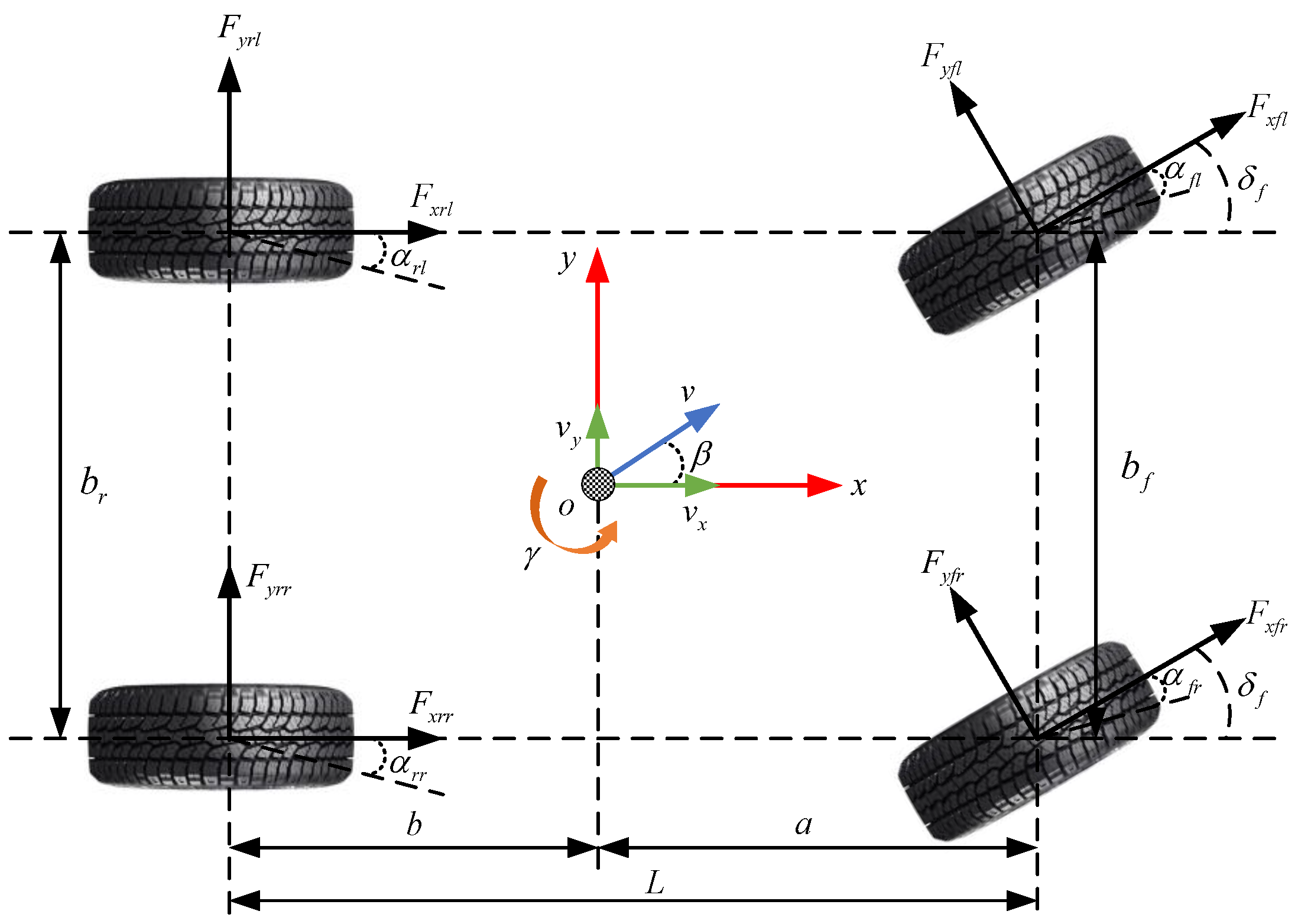
Figure 1. Vehicle body dynamics model.
Mathematics 14 00183 g001
Figure 2. Wheel rotational dynamics model.
Mathematics 14 00183 g002
Figure 3. 7-DOF full vehicle model architecture.
Mathematics 14 00183 g003
Figure 4. RF algorithm feature importance scores.
Mathematics 14 00183 g004
Figure 5. BPNN training results.
Mathematics 14 00183 g005
Figure 6. PCC correlation value.
Mathematics 14 00183 g006
Figure 7. PCC significance value.
Mathematics 14 00183 g007
Figure 8. Sideslip angle redundant estimation scheme.
Mathematics 14 00183 g008
Figure 9. β redundancy estimation results under the DLC scenario. (a) Vehicle speed 72 km/h, μ = 0.7; (b) Vehicle speed 36 km/h, μ = 0.4.
Mathematics 14 00183 g009
Figure 10. Sideslip angle β redundancy estimation results under the Slalom scenario. (a) Vehicle speed 72 km/h, μ = 0.7; (b) Vehicle speed 36 km/h, μ = 0.4.
Mathematics 14 00183 g010
Table 1. In-Wheel Motor Performance Parameters.
ParameterPeak TorqueRated TorqueRated PowerMaximum Speed
Value1250 N·m650 N·m54 kW1600 r/min
Table 2. Specific data collection scenarios.
Collection ConditionsRoad AdhesionSpeed Range (km/h)
DLC0.320–60
DLC0.520–70
DLC0.8520–130
Slalom0.320–40
Slalom0.520–60
Slalom0.8520–70
Table 3. Vehicle parameters.
ParameterValue
Vehicle mass m/kg1501
Distance from the vehicle’s center of gravity to front axle a/m1.015
Distance from the vehicle’s center of gravity to rear axle b/m1.895
Height of the center of gravity hg/m0.54
Front track width df/m1.675
Rear track width dr/m1.675
Yaw moment of inertia Iz/(kg·m2)1536.7
Effective tire radius R/m0.325
Wheel moment of inertia J/(kg·m2)1.5
Table 4. Sideslip angle redundancy estimation results under DLC condition.
Performance MetricsDLC
μ = 0.7μ = 0.4
MaxAE0.52950.1855
MAE0.03400.0332
RMSE0.08160.0466
Table 5. Sideslip angle redundancy estimation results under slalom condition.
Performance MetricsSlalom
μ = 0.7μ = 0.4
MaxAE1.28330.5551
MAE0.10370.0286
RMSE0.24080.0539
Disclaimer/Publisher’s Note: The statements, opinions and data contained in all publications are solely those of the individual author(s) and contributor(s) and not of MDPI and/or the editor(s). MDPI and/or the editor(s) disclaim responsibility for any injury to people or property resulting from any ideas, methods, instructions or products referred to in the content.