Pricing Optimization for Inventory with Integrated Storage and Credit Constraints

Abstract

Price is a pivotal determinant of market demand, as higher prices typically reduce sales while lower prices stimulate them. Thus, incorporating price-dependent demand into inventory models is both realistic and necessary. In practice, limited storage capacity often forces retailers to rent additional space, motivating the adoption of two-warehouse systems. Trade credit also plays a critical role in supply chain management: suppliers may offer cash discounts or deferred payments to encourage larger orders, while retailers extend credit to customers to boost sales. To reduce default risk, however, retailers usually provide only partial credit. Considering the time value of money, costs and profits are assessed using discounted cash-flow analysis to account for payment delays and inflation. This study develops an integrated supplier–retailer–customer chain model that (1) incorporates price-dependent demand, (2) includes a rented warehouse for limited storage, (3) considers partial trade credit, (4) links two-level trade credit terms to order quantity, and (5) evaluates financial performance on a present-value basis. The model aims to maximize total profit by determining optimal price, replenishment cycle, and order quantity. Numerical and sensitivity analyses confirm that extending supplier credit can lower prices and improve overall profitability, offering useful insights for strategic inventory management.

1. Introduction

In the early development of the Economic Order Quantity (EOQ) model, the demand rate was predominantly assumed to be constant. The EOQ model provides a foundational framework for determining the optimal order size that minimizes the combined costs of holding and ordering inventory. Although the model assumes stable demand, fixed lead times, and no quantity discounts, its core logic remains highly relevant to real-world supply chain challenges. Subsequent research, however, extended this framework by incorporating time-varying demand structures, such as linear, quadratic, exponential, and other functional forms. Parallel to this progression, studies on deteriorating items have typically characterized deterioration as either constant or time-dependent, frequently modeled through exponential decay functions or Weibull distributions. As products undergo gradual deterioration, expiration dates (or sell-by dates) are established, beyond which the items lose marketability. Even if demand structures have changed, EOQ still provides a baseline for understanding these trade-offs and supports practical decisions, such as setting replenishment frequencies, coordinating purchasing activities, and evaluating the impact of uncertainty on inventory performance. However, organizations must balance cost efficiency with service-level requirements, manage space and cash-flow constraints, and respond to demand and supply variability. Even as modern supply chains grow more complex, EOQ remains theoretically significant and practically relevant as both an instructional model and a diagnostic tool for analyzing inventory management challenges.

In practice, price is a key determinant of market demand, as higher prices typically lead to lower sales. Modeling demand as a function of price is, therefore, both necessary and practical. Limited storage capacity adds complexity to inventory decisions, often prompting retailers to rent additional space and adopt a two-warehouse system. Suppliers may offer cash discounts or deferred payments for large orders, while retailers extend trade credit to customers. To mitigate default risk, however, retailers usually provide only partial credit. Furthermore, costs and profits are evaluated on a present-value basis, capturing the effects of time and inflation. Together, these factors represent important and practically relevant considerations in designing effective inventory management policies.

This study develops a supplier–retailer–customer supply chain model that incorporates five critical factors influencing inventory management: price-dependent demand, limited storage capacity, partial trade credit, order quantity–linked trade credit, and discounted cash flow. A review of the relevant literature is presented in Section 2 to provide context for the present study.

Yang [1] developed an inventory model that considers item deterioration and demand variability, while simultaneously incorporating limited storage capacity and downstream partial trade credit linked to the order quantity, using a discounted cash flow (DCF) framework. The inventory system examined in this research follows the framework of Yang [1] and simultaneously incorporates five critical factors. Specifically: (1) the demand rate is assumed to be price-dependent, (2) storage capacity is constrained, necessitating consideration of limited warehouse space, (3) the downstream trade credit is structured as partial to mitigate default risk, (4) a two-level trade credit scheme is adopted, with credit terms linked to the order quantity, and (5) the influence of inflation and the time value of money is captured through DCF analysis. Furthermore, unlike Yang [1], this study explicitly focuses on profit maximization, aiming to determine the optimal selling price and replenishment cycle that maximizes the present value of total profit per unit of time. This modification provides a more accurate reflection of real market conditions and trading dynamics. To illustrate the model’s applicability, numerical examples are provided, followed by managerial insights. Moreover, a sensitivity analysis is performed to examine how variations in critical parameters affect the optimal policy derived.

The rest of the paper is structured as follows. Section 2 presents a review of the relevant literature. The assumptions and notation used are described in Section 3. The models developed and discussed are in Section 4 and Section 5, respectively. Section 6 and Section 7 present numerical examples to illustrate the results and conduct sensitivity analysis. Finally, a conclusion is drawn from the managerial insights and future directions presented in Section 8.

2. Literature Review

The subsequent five subsections provide a concise review of the relevant literature to contextualize the current study.

2.1. Research on Price-Dependent Demand

In actual applications, the demand rate for certain products—particularly new, high-tech, or fashionable items—is strongly influenced by the selling price. To address this, various studies have developed inventory and pricing models incorporating price-dependent demand. For example, Alfares and Ghaithan [2] introduced a mathematical model addressing the interaction among price-dependent demand, dynamic holding costs, and quantity discount mechanisms. Feng et al. [3] proposed decision-making frameworks for perishable goods that integrate price-sensitive demand, inventory display levels, and expiration dates to guide pricing and lot-sizing policies. Giri et al. [4] investigated optimal payment timing in a two-echelon supply chain, and Rameswari and Uthayakumar [5] formulated a comprehensive model for managing deteriorating items with price-dependent demand under a two-level trade credit policy. Extending this line of research, Li et al. [6] explored optimal credit terms, order quantities, and pricing policies for perishable products, considering price, expiration dates, and credit periods. In a stochastic environment, Giri and Masanta [7] developed a closed-loop supply chain model with price- and quality-dependent demand and learning in production. Li et al. [8] further addressed lot-sizing and pricing decisions for perishable products in three-echelon supply chains, where demand is dependent on price and stock age. Feng et al. [9] examined how unit price, display quantity, and product age jointly affect the demand and corresponding pricing and lot-sizing decisions for fresh goods under generalized payment terms. Taleizadeh et al. [10] introduced a sustainable inventory framework that accounts for price-dependent demand, carbon emissions, and partial trade credit under the condition of partial backlogging. Meanwhile, Yang and Liu [11] proposed and evaluated price-timing financing strategies tailored to supply chains with limited capital resources and price-dependent stochastic demand. Other notable studies that consider the price-dependent demand include the works of Das et al. [12], Tayal et al. [13], Bai et al. [14], Kausar et al. [15], Pal et al. [16], Lin et al. [17], Liu et al. [18], and Sharma et al. [19].

2.2. Analysis of Limited Storage Capacity

In practical situations, as the order quantity exceeds the retailer’s own storage capacity, it becomes necessary to rent an additional warehouse, reflecting the constraint of limited storage capacity. This issue has been addressed by numerous studies in the literature. For instance, Lin et al. [20] proposed a decision-making framework for inventory management of two-stage deteriorating products that integrates trade credit and adjustable capacity utilization. Shekarabi et al. [21] contributed to the field by introducing a generalized outer approximation approach that enables the optimization of lot-sizing policies in complex integrated supply chains involving multiple levels and wholesalers, while simultaneously considering shortage risks and warehouse space restrictions. Yen et al. [22] proposed an Economic Production Quantity (EPQ) model integrating raw material deterioration, storage limitations, and holding costs within the context of two-level trade credit financing. Yang [23] developed a retailer’s ordering policy considering expiration-date-dependent demand under limited storage and supplier credits tied to order quantity with discounted cash flow. Duary et al. [24] developed a price-discount inventory model for deteriorating products, incorporating both advance and delayed payment schemes, capacity limitations, and partially backlogged shortages. Sicilia et al. [25] formulated an optimal decision-making model for managing multi-item systems with random demand, backlogged shortages, and constrained storage capacity, while Ambroszkiewicz and Bylka [26] examined relatively optimal stock management policies in supply chains where inventory space is restricted. Zhang et al. [27] discussed the pricing decision of a capacity-sharing supply chain under information asymmetry.

2.3. Partial Trade Credit in Research

The provision of trade credit introduces not only additional financing costs for suppliers but also a heightened risk of customer default. To mitigate such risks while still promoting sales, retailers may adopt a partial downstream trade credit strategy. Under this policy, customers are required to pay a portion of the product price upon receipt, with the remaining balance payable within a specified credit period. This arrangement strikes a balance between stimulating demand and mitigating default risk. The concept of partial trade credit was formalized in the inventory literature by Huang and Hsu [28], who developed an EOQ model incorporating a retailer’s partial trade credit policy within a supply chain context. Thangam and Uthayakumar [29] extended this framework to a two-warehouse system for deteriorating items under partial trade credit financing, demonstrating the interaction between storage constraints and credit policies. Further developments include Chen et al. [30], who examined an EPQ model combining upstream full trade credit with downstream partial trade credit, and Wu and Chan [31], who considered lot-sizing policies for deteriorating items with expiration dates when serving credit-risk customers. Building on these foundations, Wu et al. [32] analyzed a practical inventory model for perishable items under downstream partial trade credit, using discounted cash-flow techniques to guide decision-making. Shah et al. [33] contributed by analyzing inventory policies for deteriorating products, considering quadratic demand patterns and integrating two-tier trade credit schemes, namely full credit from suppliers and partial credit to buyers, while Tiwari et al. [34] proposed a practical decision-making framework for deteriorating goods, integrating joint pricing, inventory control, partial backlogging, and two-level trade credit mechanisms. Similarly, Giri and Sharma [35] proposed a practical framework for managing production and inventory systems under cash discount incentives and partial trade credit conditions, and Li et al. [6] developed models to determine optimal credit terms, order quantities, and pricing policies for perishable products where demand depends jointly on price, expiration date, and credit period. More recent contributions have advanced the complexity of such models. Mahata et al. [36] analyzed EOQ models for time-varying deteriorating items under two-level partial trade credit, while Taleizadeh et al. [37] addressed inventory policies in mixed-sale environments with inspection, multiple pre-payments, partial credit, and order-quantity-linked payments under full backordering. Taleizadeh et al. [38] analyzed how partial order-linked credit and product lifetime influence the optimal ordering policy for decaying items. Most recently, Chang et al. [39] introduced perishable inventory models in which suppliers employ an advance-cash-credit payment scheme to retailers, who in turn adopt a cash–credit policy toward customers, incorporating partial backlogging. Collectively, these studies underscore the growing recognition of partial trade credit as a vital mechanism for mitigating financial risk, influencing customer behavior, and enhancing supply chain performance. Interesting and relevant studies related to partial trade credit include those by Shah et al. [33], Das et al. [40], Xu and Fang [41], Zou and Tina [42], Dai and Wang [43], Moradi et al. [44], and Choudhury and Mahata [45].

2.4. Analysis of Trade Credit Dependent on Order Quantity

To stimulate larger purchases, suppliers frequently offer retailers a conditional permissible delay in payment when the order quantity exceeds a predetermined threshold. This order-quantity-linked trade credit policy has attracted significant scholarly attention due to its practical relevance and its impact on both inventory and financing decisions. Ouyang et al. [46] first investigated this issue by developing an EOQ model for deteriorating items under a permissible delay in payments linked to order quantity. Kreng and Tan [47] extended this work by proposing an inventory model with two levels of trade credit, both of which are dependent on the order size, thereby demonstrating how order-linked credit can coordinate supplier–retailer relationships. Shah and Cárdenas-Barrón [48] examined retailer decision-making for deteriorating items when suppliers offered either order-size-dependent credit or cash discounts, emphasizing the strategic interplay between credit terms and pricing incentives. In a related contribution, Tiwari et al. [49] formulated an optimal inventory policy for deteriorating items, explicitly incorporating order-size-linked trade credit and full backlogging, highlighting the influence of shortages and customer waiting behavior. Tsao et al. [50] analyzed how order-linked trade credit influences the optimal pricing, ordering quantity, and credit period decisions for deteriorating products. Interesting and relevant studies related to trade credit dependent on order quantity include those by Chung et al. [51] and Tayal et al. [13]. Collectively, these studies demonstrate the significant role of order-quantity-linked trade credit in aligning supplier incentives with retailer purchasing strategies, while also incorporating complex real-world features such as deteriorating demand, backlogging, and multi-level credit structures.

2.5. Research on Discounted Cash Flow

In contemporary competitive markets, inventory-related costs are substantially influenced by inflation and the time value of money. Thus, it is essential to account not only for the opportunity cost of trade credit but also for the impact of these financial factors on all cost components. To this end, several studies have applied the DCF approach in inventory modeling. Building on this foundation, Chen and Teng [52] developed inventory and credit decision models for time-varying deteriorating items with both upstream and downstream trade credit financing. Shah and Cárdenas-Barrón [48] developed models to evaluate retailer ordering and financing decisions for deteriorating goods in the presence of supplier-provided order-based credit and cash discount policies. Extending this line of research. More recent contributions have considered increasingly complex environments. Yang [1] formulated an inventory model that accounts for the deterioration of items and the effects of demand fluctuations, simultaneously incorporating limited storage capacity and downstream partial trade credit linked to order quantity through DCF analysis. Yang et al. [53] proposed an optimal replenishment strategy for high-tech products subject to non-instantaneous deterioration under an advance-cash-credit payment scheme, which was also evaluated using the DCF analysis. Similarly, Chang and Tseng [54] formulated EOQ models for perishable products that jointly account for advance-cash-credit schemes and carbon emission policies, thereby extending the applicability of DCF-based models to sustainability concerns. Several other noteworthy and pertinent studies on discounted cash flow have been conducted, including those by Wu et al. [32], Sutjipto et al. [55], Viswanath et al. [56], Pal et al. [15], Pathak et al. [57], and Tsao et al. [58].

A summary of these key contributions is presented in

Table 1. Key Characteristics of Selected Inventory Models.

Authors	Demand Pattern	Limited Storage Capacity	Partial Trade Credit	Dependent on Order Quantity	Discounted Cash-Flow
Huang and Hsu [28]	Constant		V
Ouyang et al. [46]	Constant			V
Kreng and Tan [47]	Constant			V
Thangam and Uthayakumar [29]	Price-dependent	V	V
Chen et al. [30]	Production inventory		V
Wu and Chan [31]	Constant		V
Chen and Teng [52]	Constant				V
Shah and Cárdenas-Barrón [48]	Credit-dependent			V	V
Alfares and Ghaithan [2]	Price-dependent
Wu et al. [32]	Constant		V		V
Feng et al. [3]	Price, stock, and expiration date dependent
Giri et al. [4]	Price-dependent
Rameswari and Uthayakumar [5]	Price-dependent
Shah et al. [33]	Quadratic demand		V
Tiwari et al. [34]	Price-dependent		V
Giri and Sharma [35]	Production-inventory		V		V
Li et al. [6]	Price and credit dependent		V		V
Lin et al. [20]	Constant	V
Shekarabi et al. [21]	Multi-product	V
Yen et al. [22]	Production-inventory	V			V
Giri and Masanta [7]	Price-dependent
Mahata et al. [36]	Credit period-dependent		V
Taleizadeh et al. [37]	Decreasing demand		V	V
Tiwari et al. [49]	Constant			V
Li et al. [10]	Price and stock-age dependent
Taleizadeh et al. [38]	Lifetime dependent		V	V
Yang [23]	Expiration-date dependent	V		V	V
Feng et al. [9]	price, stocks, and product age dependent
Sicilia et al. [25]	Stochastic demand	V
Taleizadeh et al. [10]	Price- sensitive demand		V
Tsao et al. [50]	EOQ			V	V
Ambrosz-kiewicz and Bylka [26]	Constant	V
Yang [1]	Fluctuating demand	V	V		V
Yang and Liu [11]	Price-dependent stochastic demand
Chang and Tseng [54]	Price-expiration-date dependent		V		V
Yang et al. [53]	Ramp-type				V
Chang et al. [39]	Constant		V
This paper	Price-dependent	V	V	V	V

Note: The symbol “V” denotes that it satisfies the header condition.

.

3. Assumptions and Notation

The assumptions used in this research are similar to those of Yang [1]. Briefly, the owner’s warehouse, OW, has a fixed capacity, $W$, whereas the rented warehouse, RW, has unlimited capacity. If the order quantity $Q$ exceeds the $W$, then the retailer will rent a warehouse to store the excess items.

In addition, most of the notation used is the same as that used in Yang [1], except for the following.

$f\left(p\right)$	the demand rate is a function of the selling price, where a is the coefficient of the demand rate, and b is the coefficient of the selling price.
	i.e., $f\left(p\right)=a{e}^{-bp}$ where $a,b>0$.
$\alpha$	the immediate payment fraction of the total purchase cost that customers must pay upon receipt of the items.
$Q_d$	the predetermined order quantity at which the delay is permitted by the supplier.
$T_d$	the time interval that $Q_d$ units are depleted to zero due to both demand and deterioration.
$T{P}_{ij}\left(p,T\right)$	the discounted total profit per unit time, which is a function of p and T, where i = 1, 2, 3, 4, j = 1, 2.
${Model}_{ij}$	the model proposed corresponding to $T{P}_{ij}(p,T)$, where $i=1, 2, 3, 4$$, j=1, 2.$
$p^{*}$	the optimal selling price.
$T{P}^{*}\left(p^{*},T^{*}\right)$	the optimal discounted total relevant profit per unit of time at  $T^{*}$ and $p^{*}$.

4. Research Models

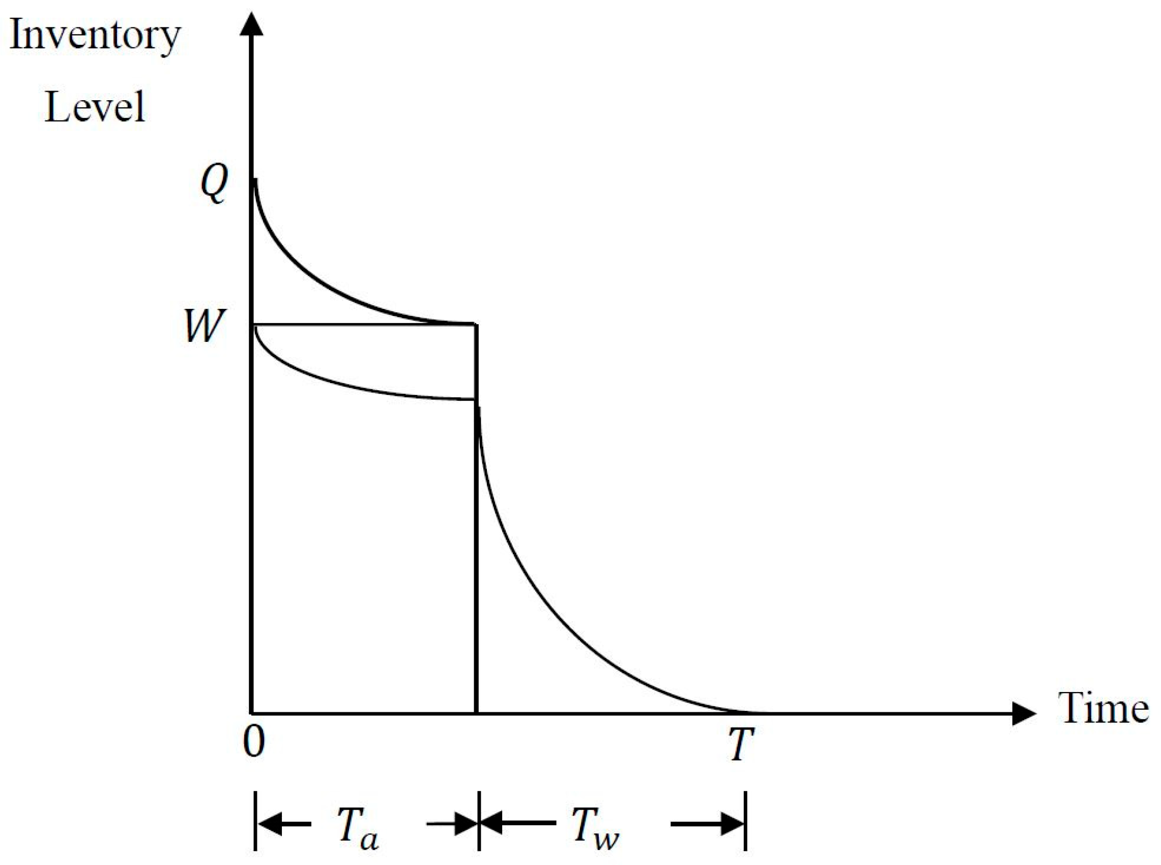
In the following, Figure 1 illustrates the inventory model graphically for the case where $Q>W$ and among them, the notation $T_a$ is the time at which the inventory level of RW reaches zero due to both demand and deterioration, and $T_a\left\{\begin{array}{c}=0, \mathrm{if} Q\le W\\ >0, \mathrm{if} Q>W\end{array}\right.$. Moreover, the notation $T_w$ is the time interval that $W$ units are depleted to zero due to both demand and deterioration.

In the model, the inventory level at time t, denoted as $I\left(t\right)$, decreases simultaneously due to demand and deterioration, where $\theta$ is the deterioration rate. The following differential equations govern the inventory level at time $t$:

$${\displaystyle \frac{dI\left(t\right)}{dt}}=-f\left(p\right)-\theta I\left(t\right), 0\le t\le T,$$

(1)

with the boundary condition $I\left(T\right)=0$. The solution to (1) is

$$I(t)=e^{-\theta t}{\int }_{ t}^{ T}{e}^{\theta u} f\left(p\right)du. 0\le t\le T,$$

(2)

Hence, the order quantity is

$$Q=I\left(0\right)=f\left(p\right){\int }_{ 0}^{ T}{e}^{\theta t}dt.$$

(3)

From (3), we get $T_d$, $T_a$ and $T_w$ by using the following equations:

$$Q_d= {\int }_{ 0}^{ T_d}{e}^{\theta t} f\left(p\right)dt.$$

(4)

$$W={\int }_{ T_a}^{ T}{e}^{\theta t} f\left(p\right)dt,$$

(5)

and

$$Q-W={\int }_{ 0}^{ T_a}{e}^{\theta t} f\left(p\right)dt, \mathrm{i}\mathrm{f} Q>W,$$

(6)

respectively. Hence, the inventory system can be decomposed into the following constituent elements.

(a)

The ordering cost is A.

(b)

The notations $h$ and $k$ are the holding cost per unit of time, excluding interest charge in OW and RW, respectively. If $Q\le W$, then the inventory holding cost in RW and OW are

$$C_{HR}=0,$$

and

$$C_{HO}=h {\int }_{ 0}^{ T}{e}^{-rt}I\left(t\right)dt=h{\int }_{ 0}^{ T}{e}^{-(\theta +r) t} {\int }_{ t}^{ T}{e}^{\theta u} f\left(p\right)du dt .$$

(7)

If $Q>W$, then the inventory holding cost in RW and OW are

$$\begin{array}{c}{C}_{HR}=k {\int }_{ 0}^{ T_a}{e}^{-r t}\left[I\left(t\right)-W\right]dt\hfill \\ \hfill \hspace{1em} =k \left[{\int }_{ 0}^{ T_a}{e}^{-\left(\theta +r\right)t}{\int }_{ t}^{ T_a}{e}^{\theta u}f\left(p\right)du dt-W{\int }_{ 0}^{ T_a}{e}^{-r t}dt\right],\end{array}$$

and

$$C_{HO}=h \left[{\int }_{ 0}^{ T_a}W{e}^{-\left(\theta +r\right)t}dt+{\int }_{ T_a}^{ T}{e}^{-\left(\theta +r\right)t} {\int }_{ t}^{ T}{e}^{ \theta u} f\left(p\right)du dt \right].$$

(8)

Moreover, all the study’s Equations in the following are first derived except for the above Equations (1)–(8), which are leveraged from the previous one as Yang [1].

(c)

The notation $c$ is the unit purchasing cost. Then the deterioration cost is

$$C_D=\theta c{\int }_{ 0}^{ T}{e}^{-rt}I\left(t\right)dt$$

(d)

The purchasing cost is

$$C_P=c{\int }_{ 0}^{ T}f\left(p\right)e^{-rt}dt=cf\left(p\right){\displaystyle \frac{1-e^{-rT}}{r}}$$

(e)

The realized revenue is

$$R=p{\int }_{ 0}^{ T}f\left(p\right)e^{-rt}dt=pf\left(p\right){\displaystyle \frac{1-e^{-rT}}{r}}$$

4.1. $Q<Q_d$

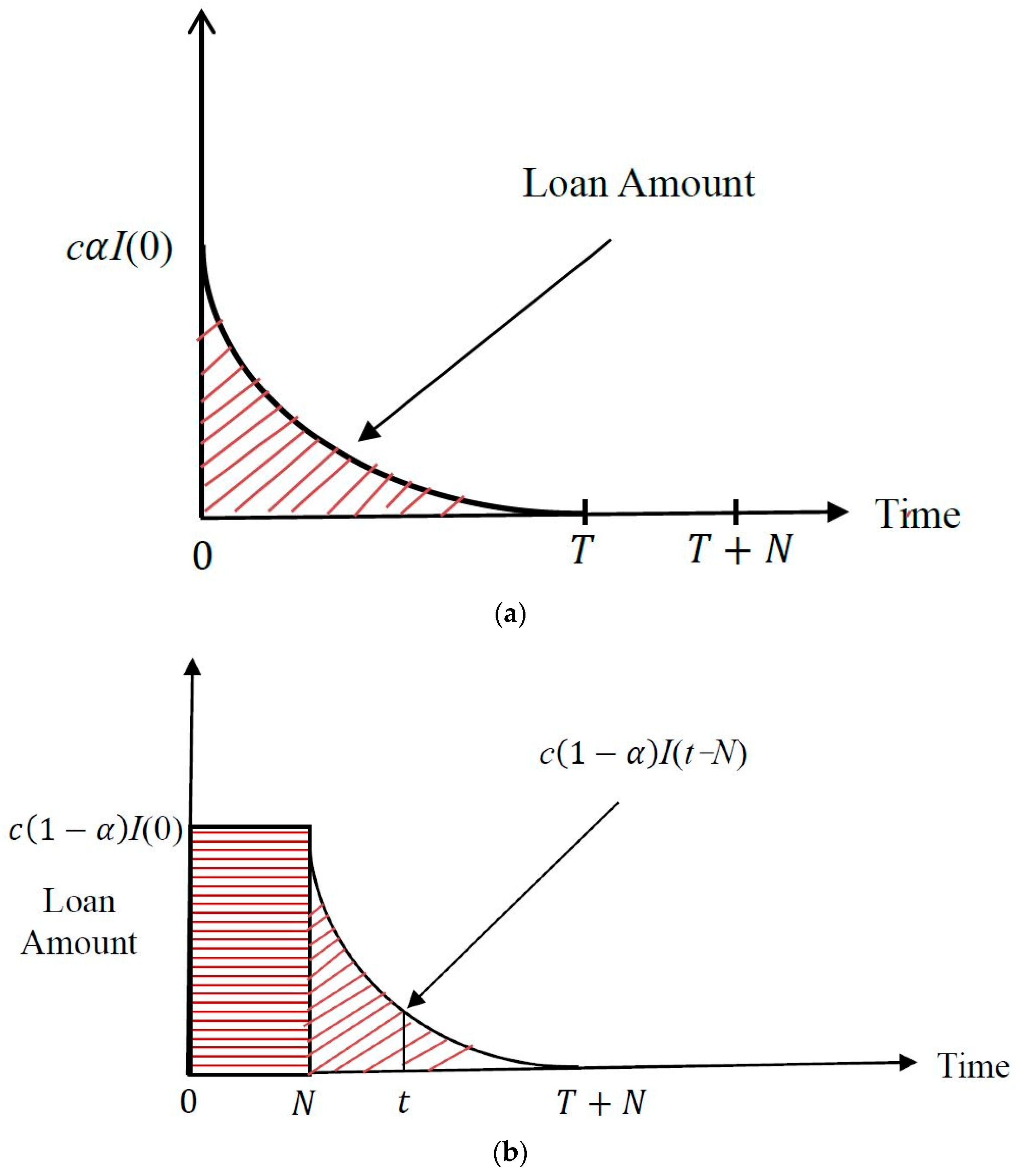
In the following, we define $M$ as the retailer’s trade credit period, as offered by the supplier, in years. And $N$ is the customer’s trade credit period, as offered by the retailer, in years. Now, with an order quantity $Q$ less than $Q_d$ and $T<T_d$, the retailer cannot allow any delay in payment (i.e., $M=0$), and no interest earned is generated by credit. At the same time, the retailer extends a partial permissible delay of $N$ to its customers. Thus, the retailer must cover (i) cash payments from time $0$ to $T$ and (ii) credit payments from $0$ to $N$ and $N$ to $T+N$, as indicated in Figure 2a (red slash line region) and Figure 2b (red horizontal and slash line regions). Consequently, the discounted interest paid by the retailer is

$$\begin{array}{c}\hfill IP=c{I}_p\left\{\alpha {\int }_{ 0}^T{e}^{-rt}I\left(0\right)dt +\left(1-\alpha \right)\left[{\int }_{ 0}^{ N}{e}^{-rt}I\left(0\right)dt+{\int }_{ N}^{ T+N}{e}^{-r\left(t-N\right)}I\left(t-N\right)dt \right]\right\}\hfill \\ =c{I}_p\left\{\alpha {\int }_0^T{e}^{-rt}{\int }_{ 0}^{ T}{e}^{\theta u}f\left(p\right)du dt\right.+\left(1-\alpha \right)\left[{\int }_0^N{e}^{-rt}{\int }_{ 0}^{ T}{e}^{\theta u}f\left(p\right)du dt\right.\hfill \\ \left.\left.+{\int }_{ N}^{ T+N}{e}^{-\left(\theta +r\right)\left(t-N\right)}{\int }_{ t-N}^{ T}{e}^{\theta u}f\left(p\right)du dt\right]\right\}\hfill \end{array}$$

Thus, based on the above discussions, the discounted total profit per unit time for the retailer to be maximized is

$$TP\left(p,T\right)={\displaystyle \frac{1}{T}}\left(R-A-C_{HO}-C_{HR}-C_D-C_P-IP+IE\right).$$

(9)

Next, two subcases are considered, depending on whether the order quantity exceeds the capacity of own warehouse: (i) $Q\le W$ (ii) $Q>W$. Then, the discounted total profit per unit time $T{P}_{1j}\left(p,T\right)$ of model ${Model}_{1j}, j=1,2$, are obtained as follows:

$$\begin{array}{c}T{P}_{11}\left(p,T\right)={\displaystyle \frac{1}{T}}\left\{\left(p-c\right)f\left(p\right){\displaystyle \frac{1-e^{-rT}}{r}}\right.\hfill \\ -\left\{A+\left(h+\theta c\right){\int }_{ 0}^{ T}{e}^{-\left(\theta +r\right)t}{\int }_{ t}^{ T}{e}^{\theta u} f\left(p\right)du dt+c{I}_p\left[\alpha {\int }_0^T{e}^{-rt}{\int }_{ 0}^{ T}{e}^{\theta u}f\left(p\right)du dt\right.\right.\hfill \\ \left.\left.\left. +\left(1-\alpha \right)\left[{\int }_0^N{e}^{-rt}{\int }_{ 0}^{ T}{e}^{\theta u}f\left(p\right)du dt+{\int }_{ N}^{ T+N}{e}^{-\left(\theta +r\right)\left(t-N\right)}{\int }_{ t-N}^{ T}{e}^{\theta u}f\left(p\right)du dt\right]\right]\right\}\right\}, \mathrm{i}\mathrm{f} Q\le W.\hfill \end{array}$$

(10)

$$\begin{array}{c}T{P}_{12}\left(p,T\right)={\displaystyle \frac{1}{T}}\left\{\left(p-c\right)f\left(p\right){\displaystyle \frac{1-e^{-rT}}{r}}-\left\{A+\theta c{\int }_{ 0}^{ T}{e}^{-\left(\theta +r\right)t}{\int }_{ t}^{ T}{e}^{\theta u} f\left(p\right)du dt\right.\right.\hfill \\ +h \left[{\int }_{ 0}^{ T_a}W{e}^{-\left(\theta +r\right)t}dt+{\int }_{ T_a}^{ T}{e}^{-\left(\theta +r\right)t} {\int }_{ t}^{ T}{e}^{ \theta u} f\left(p\right)du dt \right]\hfill \\ +k \left[{\int }_{ 0}^{ T_a}{e}^{-\left(\theta +r\right)t}{\int }_{ t}^{ T_a}{e}^{\theta u}f\left(p\right)du dt-W{\int }_{ 0}^{ T_a}{e}^{-rt}dt\right]+c{I}_p\left[\alpha {\int }_0^T{e}^{-rt}{\int }_{ 0}^{ T}{e}^{\theta u}f\left(p\right)du dt\right.\hfill \\ \left.\left.\left. +\left(1-\alpha \right)\left[{\int }_0^N{e}^{-rt}{\int }_{ 0}^{ T}{e}^{\theta u}f\left(p\right)du dt+{\int }_{ N}^{ T+N}{e}^{-\left(\theta +r\right)\left(t-N\right)}{\int }_{ t-N}^{ T}{e}^{\theta u}f\left(p\right)du dt\right]\right]\right\}\right\}, if Q>W.\hfill \end{array}$$

(11)

4.2. $Q\ge Q_d$

Under this scenario, the order quantity $Q$ is at least $Q_d$ and $T\ge T_d$. The retailer faces three potential options for the replenishment cycle $T$, determined by the supplier’s trade credit $M$ and the final customer payment time $T + N$: (1) $0<M<N$ (2) $0<N\le M$ and $M\le T+N$ (3) $0<N\le M$ and $M>T+N$.

4.2.1. $0<M<N$

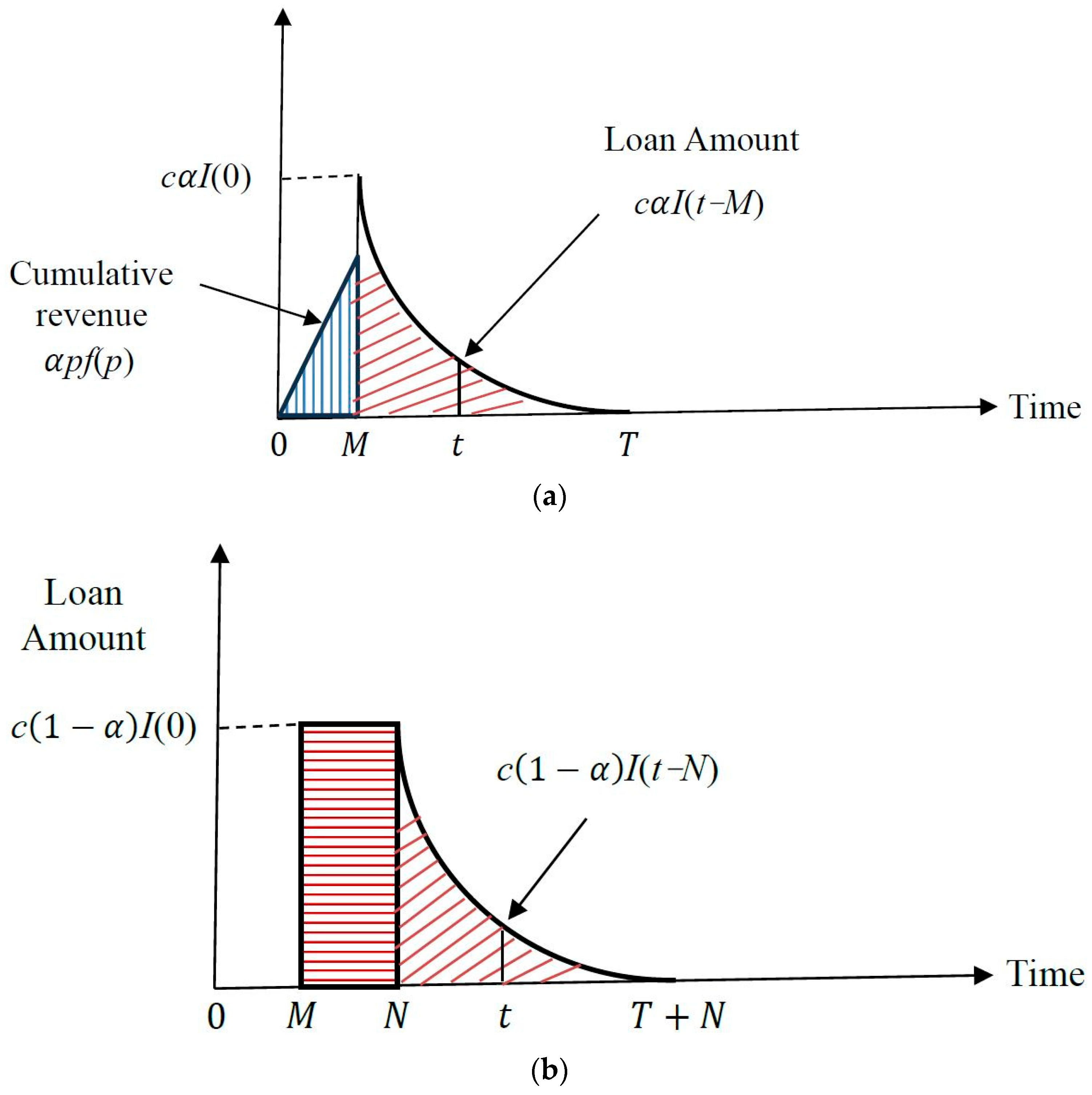
Since $M<N$, the interest is not earned from credit payments; meanwhile, the retailer receives interest from cash payments made between time $0$ and $M$, as illustrated in Figure 3a (blue vertical line region). Thus, the discounted interest earned per cycle from cash payments is

$$IE=p{I}_e\alpha {\int }_{ 0}^{ M}{e}^{-rt}{\int }_{ 0}^{ t}f\left(p\right)du dt.$$

In addition, the retailer is required to finance (i) cash payments from M to T and (ii) credit payments from M to N and N to T + N, as illustrated in Figure 3a (red slash line region) and Figure 3b (red horizontal and slash line region). Thus, the discounted interest paid by the retailer is

$$\begin{array}{c}IP=c{I}_p\left\{\alpha {\int }_{ M}^{ T}{e}^{-r\left(t-M\right)}I\left(t-M\right)dt\right.\hfill \\ \left. +\left(1-\alpha \right)\left[{\int }_{ M}^{ N}{e}^{-r\left(t-M\right)}I\left(0\right)dt + {\int }_{ N}^{ T+N}{e}^{-r(t-N)}I(t-N)dt\right]\right\}\hfill \\ =c{I}_p\left\{\alpha {\int }_M^T{e}^{-\left(\theta +r\right)\left(t-M\right)}{\int }_{ t-M}^{ T}{e}^{\theta u}f\left(p\right)du dt\right.\hfill \\ \left. +\left(1-\alpha \right)\left[{\int }_{ M}^{ N}{e}^{-r\left(t-M\right)}{\int }_{ 0}^{ T}{e}^{\theta u}f\left(p\right)du dt+{\int }_{ N}^{ T+N}{e}^{-(\theta +r)(t-N)}{\int }_{ t-N}^{ T}{e}^{\theta u}f\left(p\right)du dt\right]\right\}.\hfill \end{array}$$

Hence, based on the values of $Q$ and $W$, the discounted total profit per unit time $T{P}_{2j}\left(p,T\right)$ of model ${Model}_{2j}, j=1, 2$, are obtained as follows:

$$\begin{array}{c}T{P}_{21}\left(p,T\right)={\displaystyle \frac{1}{T}}\left\{(p-c)f\left(p\right){\displaystyle \frac{1-e^{-rT}}{r}}+p{I}_e\alpha {\int }_{ 0}^M{e}^{-rt}{\int }_0^{t}f\left(p\right)du dt \right.\hfill \\ -\left\{A+\left(h+\theta c\right){\int }_{ 0}^{ T}{e}^{-\left(\theta +r\right)t}{\int }_{ t}^{ T}{e}^{\theta u} f\left(p\right)du dt+c{I}_p\left[\alpha {\int }_M^T{e}^{-\left(\theta +r\right)\left(t-M\right)}{\int }_{ t-M}^{ T}{e}^{\theta u}f\left(p\right)du dt\right.\right.\hfill \\ \left.\left.\left. +\left(1-\alpha \right)\left[{\int }_M^N{e}^{-r\left(t-M\right)}{\int }_{ 0}^{ T}{e}^{\theta u}f\left(p\right)du dt+{\int }_{ N}^{ T+N}{e}^{-\left(\theta +r\right)\left(t-N\right)}{\int }_{ t-N}^{ T}{e}^{\theta u}f\left(p\right)du dt\right]\right]\right\}\right\}, \mathrm{i}\mathrm{f} Q\le W.\hfill \end{array}$$

(12)

$$\begin{array}{c}T{P}_{22}\left(p,T\right)={\displaystyle \frac{1}{T}}\left\{\left(p-c\right)f\left(p\right){\displaystyle \frac{1-e^{-rT}}{r}}+p{I}_e\alpha {\int }_{ 0}^M{e}^{-rt}{\int }_0^{t}f\left(p\right)du dt \right.\hfill \\ -\left\{A+\theta c{\int }_{ 0}^{ T}{e}^{-\left(\theta +r\right)t}{\int }_{ t}^{ T}{e}^{\theta u} f\left(p\right)du dt\right.\hfill \\ +h \left[{\int }_{ 0}^{ T_a}W{e}^{-\left(\theta +r\right)t}dt+{\int }_{ T_a}^{ T}{e}^{-\left(\theta +r\right)t} {\int }_{ t}^{ T}{e}^{ \theta u} f\left(p\right)du dt \right]\hfill \\ +k \left[{\int }_{ 0}^{ T_a}{e}^{-\left(\theta +r\right)t}{\int }_{ t}^{ T_a}{e}^{\theta u}f\left(p\right)du dt-W{\int }_{ 0}^{ T_a}{e}^{-rt}dt\right]\hfill \\ +c{I}_p\left[\alpha {\int }_M^T{e}^{-\left(\theta +r\right)(t-M)}{\int }_{ t-M}^{ T}{e}^{\theta u}f\left(p\right)du dt\right.\hfill \\ \left.\left.\left. +\left(1-\alpha \right)\left[{\int }_M^N{e}^{-r\left(t-M\right)}{\int }_{ 0}^{ T}{e}^{\theta u}f\left(p\right)du dt+{\int }_{ N}^{ T+N}{e}^{-\left(\theta +r\right)\left(t-N\right)}{\int }_{ t-N}^{ T}{e}^{\theta u}f\left(p\right)du dt\right]\right]\right\}\right\}, \mathrm{i}\mathrm{f} Q>W.\hfill \end{array}$$

(13)

Equations (10) and (11) can be regarded as particular instances of Equations (12) and (13) under the condition $M=0$.

4.2.2. $0<N\le M$ and $M\le T+N$

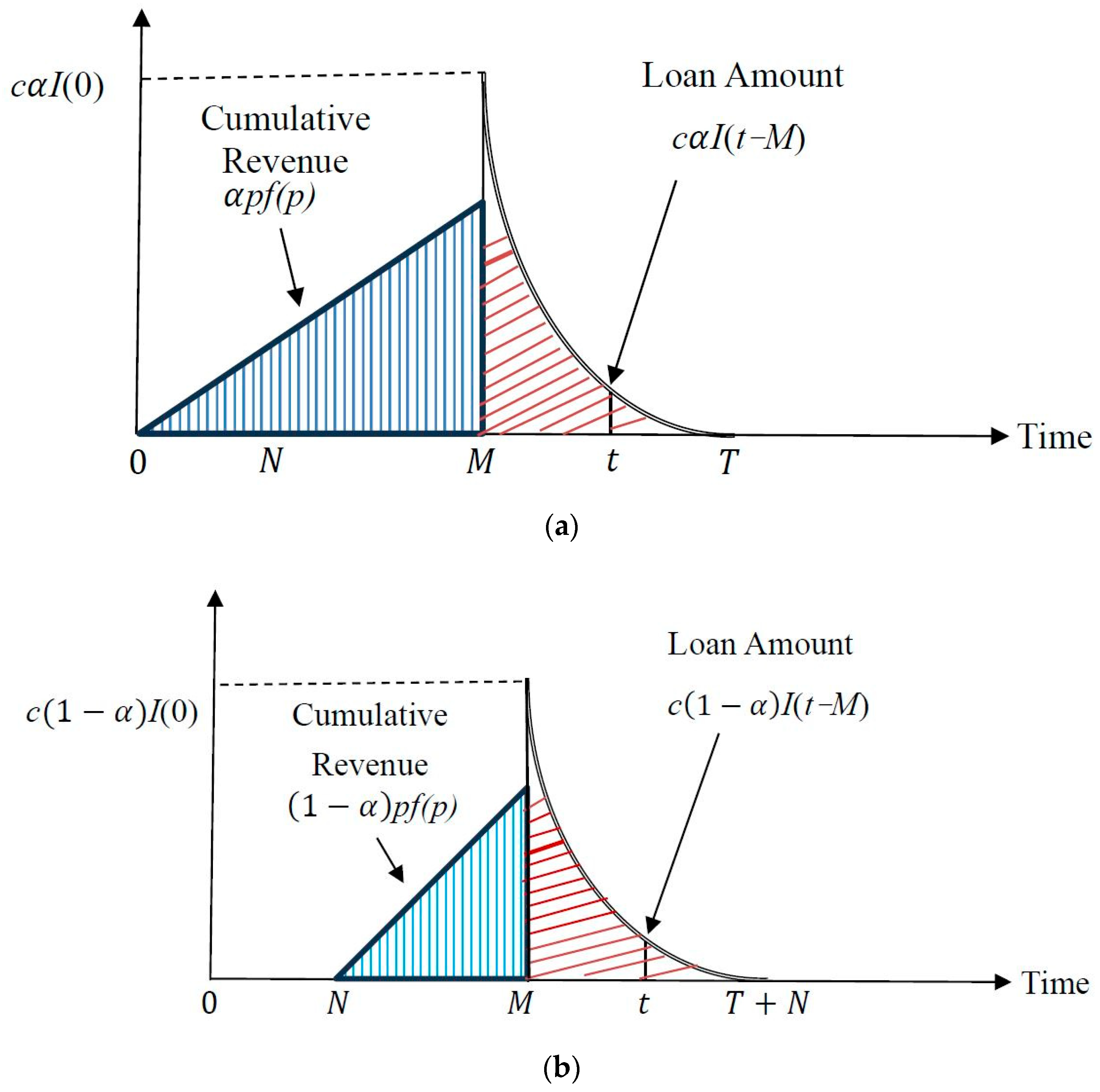
If $M\le T+N$, the retailer is unable to collect the final payment prior to the permissible delay period $M$. The retailer’s interest earnings arise from two sources: (i) cash payments received between time $0$ and $M$, and (ii) credit payments received between time $N$ and $M$, as illustrated in Figure 4a,b (blue vertical line region). Thus, the discounted interest earned per cycle by the retailer is

$$IE=p{I}_e \left[\alpha {\int }_{ 0}^{ M}{e}^{-rt}{\int }_{ 0}^{ t}f\left(p\right)du dt+\left(1-\alpha \right){\int }_{ N}^{ M}{e}^{-r\left(t-N\right)}{\int }_{ N}^{ t}f\left(p\right)du dt\right].$$

Next, the retailer charges interest on (i) cash inflows from M to T and (ii) credit inflows from $M$ to $T+N$, as shown in Figure 4a,b (red slash line region). Thus, the discounted interest paid per cycle by the retailer is

$$\begin{array}{c}IP=c{I}_p \left[\alpha {\int }_{ M}^{ T}{e}^{-r(t-M)}I\left(t-M\right)dt+\left(1-\alpha \right){\int }_{ M}^{ T+N}{e}^{-r\left(t-M\right)} I\left(t-M\right)dt\right]\hfill \\ =c{I}_p\left[\alpha {\int }_M^{ T}{e}^{-\left(\theta +r\right)(t-M)} {\int }_{ t-M}^{ T}{e}^{\theta u}f\left(p\right)du dt\right.\hfill \\ \left. +(1-\alpha ){\int }_{ M}^{ T+N} e^{-(\theta +r)(t-M)}{\int }_{ t-M}^{ T}{e}^{\theta u}f\left(p\right)du dt\right]\hfill \end{array}$$

Hence, based on the values of $Q$ and $W$, the discounted total profit per unit time $T{P}_{3j}\left(p,T\right)$ of model ${Model}_{3j}, j=1, 2$, are obtained as follows:

$$\begin{array}{c}T{P}_{31}\left(p,T\right)={\displaystyle \frac{1}{T}}\left\{\left(p-c\right)f\left(p\right){\displaystyle \frac{1-e^{-rT}}{r}}\right.\hfill \\ +p{I}_e\left[\alpha {\int }_{ 0}^{ M}{e}^{-rt}{\int }_{ 0}^{ t}f\left(p\right)du dt+\left(1-\alpha \right){\int }_{ N}^{ M}{e}^{-r\left(t-N\right)}{\int }_{ N}^{ t}f\left(p\right)du dt\right]\hfill \\ -\left\{A+\left(h+\theta c\right){\int }_{ 0}^{ T}{e}^{-\left(\theta +r\right)t}{\int }_{ t}^{ T}{e}^{\theta u} f\left(p\right)du dt\right.\hfill \\ +c{I}_p\left[\alpha {\int }_M^T{e}^{-\left(\theta +r\right)\left(t-M\right)}{\int }_{ t-M}^{ T}{e}^{\theta u}f\left(p\right)du dt\right.\hfill \\ \left.\left.\left. +\left(1-\alpha \right){\int }_M^{T+N}{e}^{-\left(\theta +r\right)\left(t-M\right)}{\int }_{ t-M}^{ T}{e}^{\theta u}f\left(p\right)du dt\right]\right\}\right\}, \mathrm{i}\mathrm{f} Q\le W.\hfill \end{array}$$

(14)

$$\begin{array}{c}T{P}_{32}\left(p,T\right)={\displaystyle \frac{1}{T}}\left\{(p-c)f\left(p\right){\displaystyle \frac{1-e^{-rT}}{r}}\right.\hfill \\ +p{I}_e\left[\alpha {\int }_{ 0}^{ M}{e}^{-rt}{\int }_{ 0}^{ t}f\left(p\right)du dt+(1-\alpha ){\int }_{ N}^{ M}{e}^{-r(t-N)}{\int }_{ N}^{ t}f\left(p\right)du dt\right]\hfill \\ -\left\{A+\theta c{\int }_{ 0}^{ T}{e}^{-\left(\theta +r\right)t}{\int }_{ t}^{ T}{e}^{\theta u} f\left(p\right)du dt\right.\hfill \\ +h \left[{\int }_{ 0}^{ T_a}W{e}^{-\left(\theta +r\right)t}dt+{\int }_{ T_a}^{ T}{e}^{-\left(\theta +r\right)t} {\int }_{ t}^{ T}{e}^{ \theta u} f\left(p\right)du dt \right]\hfill \\ +k \left[{\int }_{ 0}^{ T_a}{e}^{-\left(\theta +r\right)t}{\int }_{ t}^{ T_a}{e}^{\theta u}f\left(p\right)du dt-W{\int }_{ 0}^{ T_a}{e}^{-rt}dt\right]\hfill \\ +c{I}_p\left[\alpha {\int }_M^T{e}^{-\left(\theta +r\right)(t-M)}{\int }_{ t-M}^{ T}{e}^{\theta u}f\left(p\right)du dt\right.\hfill \\ \left.\left.\left. +\left(1-\alpha \right){\int }_M^{T+N}{e}^{-\left(\theta +r\right)(t-M)}{\int }_{ t-M}^{ T}{e}^{\theta u}f\left(p\right)du dt\right]\right\}\right\}, \mathrm{i}\mathrm{f} Q>W.\hfill \end{array}$$

(15)

4.2.3. $0<N\le M$ and $M>T+N$

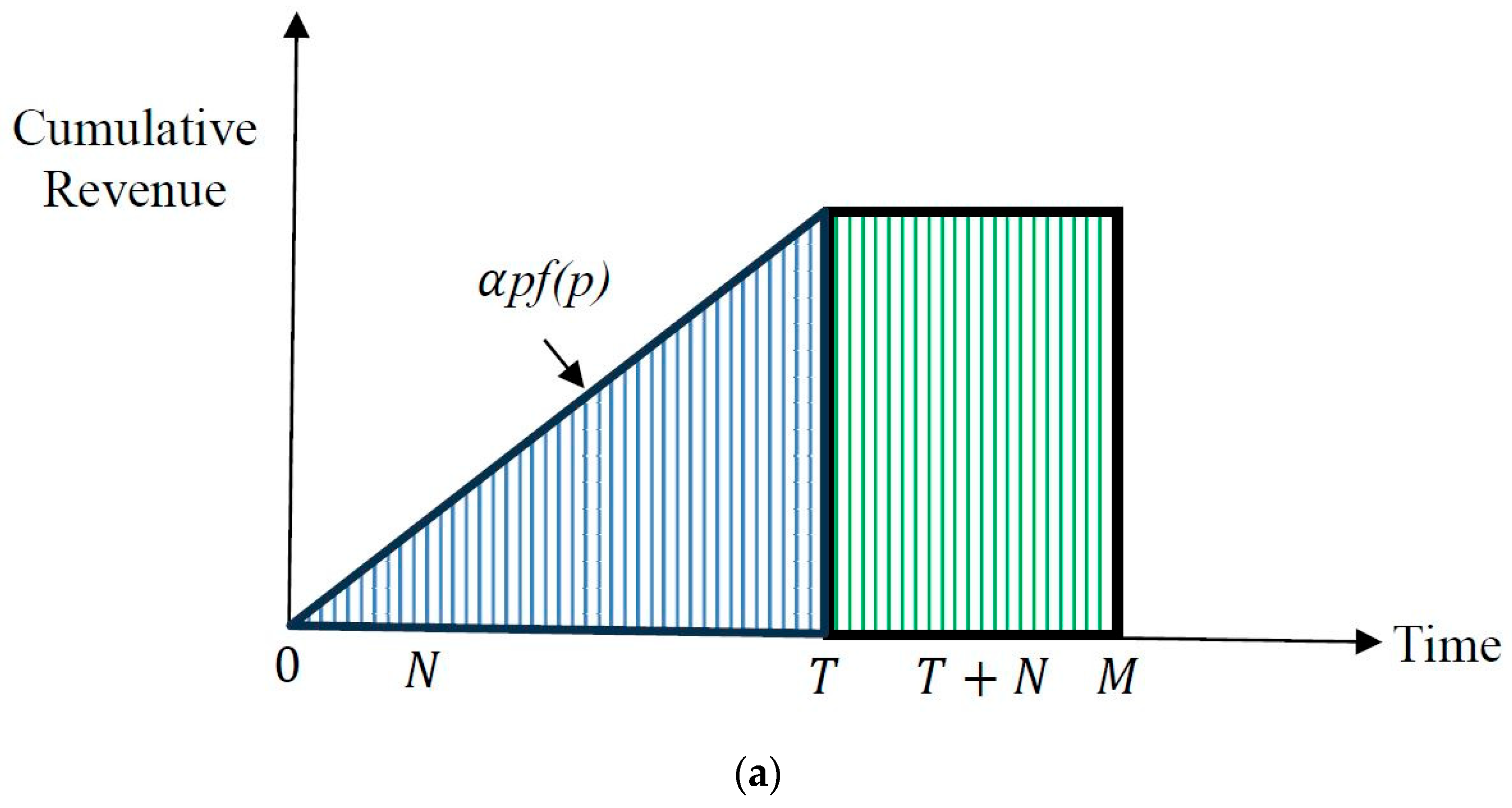
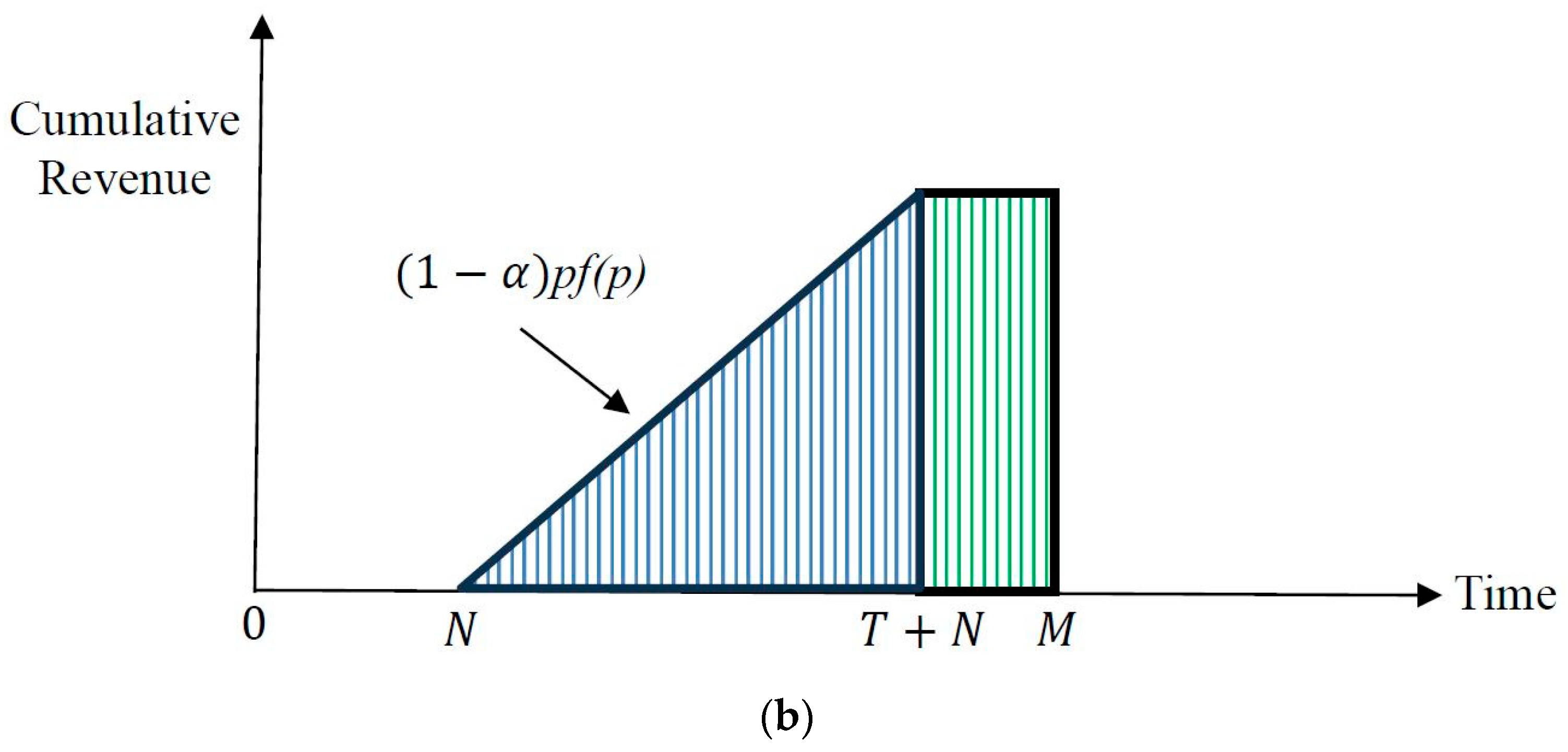
Because the order quantity $Q$ is at least $Q_d$, the retailer is granted the permissible delay in payment. When $M>T+N$, the retailer collects all customer payments by $T+N$, prior to the permissible delay $M$. Consequently, the retailer can settle the supplier’s payment at $M$ without incurring interest charges. Meanwhile, the retailer’s interest earnings arise from two sources: (i) cash inflows from $0$ to $T$ and $T$ to $M$, and (ii) credit inflows from $N$ to $T+N$ and $T+N$ to $M$, as shown in Figure 5a,b (triangular blue and rectangular green vertical line region). Hence, the discounted interest earned per cycle by the retailer is

$$\begin{array}{c}IE=p{I}_e\left\{\alpha \left[{\int }_{ 0}^{ T}{e}^{-rt}{\int }_{ 0}^{ t}f\left(p\right)du dt+{\int }_{ T}^{ M}{e}^{-r\left(t-T\right)}{\int }_{ 0}^{ T}f\left(p\right)du dt\right]\right.\hfill \\ \left. +\left(1-\alpha \right)\left[{\int }_{ N}^{ T+N}{e}^{-r\left(t-N\right)}{\int }_{ N}^{ t}f\left(p\right)du dt+{\int }_{ T+N}^{ M}{e}^{-r\left(t-T-N\right)}{\int }_{ 0}^{ T}f\left(p\right)du dt\right]\right\},\hfill \end{array}$$

and there is no interest charged; that is

$$IP=0.$$

Thus, based on the values of $Q$ and $W$, the discounted total profit per unit time $T{P}_{4j}\left(p,T\right)$ of model ${Model}_{4j}, j=1, 2$, are obtained as follows:

$$\begin{array}{c}T{P}_{41}\left(p,T\right)={\displaystyle \frac{1}{T}}\left\{(p-c)f\left(p\right){\displaystyle \frac{1-e^{-rT}}{r}}\right.\hfill \\ +p{I}_e\left\{\alpha \left[{\int }_{ 0}^{ T}{e}^{-rt}{\int }_{ 0}^{ t}f\left(p\right)du dt+{\int }_{ T}^{ M}{e}^{-r\left(t-T\right)}{\int }_{ 0}^{ T}f\left(p\right)du dt\right]\right.\hfill \\ \left. +\left(1-\alpha \right)\left[{\int }_{ N}^{ T+N}{e}^{-r\left(t-N\right)}{\int }_{ N}^{ t}f\left(p\right)du dt+{\int }_{ T+N}^{ M}{e}^{-r\left(t-T-N\right)}{\int }_{ 0}^{ T}f\left(p\right)du dt\right]\right\}\hfill \\ \left. -\left[A+\left(h+\theta c\right){\int }_{ 0}^{ T}{e}^{-\left(\theta +r\right)t}{\int }_{ t}^{ T}{e}^{\theta u} f\left(p\right)du dt\right]\right\}, \mathrm{i}\mathrm{f} Q\le W.\hfill \end{array}$$

(16)

$$\begin{array}{c}{P}_{42}\left(p,T\right)={\displaystyle \frac{1}{T}}\left\{(p-c)f\left(p\right){\displaystyle \frac{1-e^{-rT}}{r}}\right.\hfill \\ +p{I}_e\left\{\alpha \left[{\int }_{ 0}^{ T}{e}^{-rt}{\int }_{ 0}^{ t}f\left(p\right)du dt+{\int }_{ T}^{ M}{e}^{-r\left(t-T\right)}{\int }_{ 0}^{ T}f\left(p\right)du dt\right]\right.\hfill \\ \left. +\left(1-\alpha \right)\left[{\int }_{ N}^{ T+N}{e}^{-r(t-N)}{\int }_{ N}^{ t}f\left(p\right)du dt+{\int }_{ T+N}^{ M}{e}^{-r\left(t-T-N\right)}{\int }_{ 0}^{ T}f\left(p\right)du dt\right]\right\}\hfill \\ -\left\{A+\theta c{\int }_{ 0}^{ T}{e}^{-\left(\theta +r\right)t}{\int }_{ t}^{ T}{e}^{\theta u} f\left(p\right)du dt\right.\hfill \\ +h \left[{\int }_{ 0}^{ T_a}W{e}^{-\left(\theta +r\right)t}dt+{\int }_{ T_a}^{ T}{e}^{-\left(\theta +r\right)t} {\int }_{ t}^{ T}{e}^{ \theta u} f\left(p\right)du dt \right]\hfill \\ \left.\left.+k \left[{\int }_{ 0}^{ T_a}{e}^{-\left(\theta +r\right)t}{\int }_{ t}^{ T_a}{e}^{\theta u}f\left(p\right)du dt-W{\int }_{ 0}^{ T_a}{e}^{-rt}dt\right]\right\}\right\}, \mathrm{i}\mathrm{f} Q>W.\hfill \end{array}$$

(17)

5. Theoretical Results

In this Section, the theoretical results are discussed in the following two cases: (i) $Q\le W$ (ii) $Q>W$.

5.1. $Q\le W$

For $Mode{l}_{11}$, the necessary conditions for the discounted total profit function to be maximized are to take the first derivatives of $T{P}_{11}\left(p,T\right)$ with respect to $p$ and $T$, and let ${\displaystyle \frac{\partial {TP}_{11}\left(p, T\right)}{\partial p}}=0$ and ${\displaystyle \frac{\partial {TP}_{11}\left(p, T\right)}{\partial T}}=0$, we then obtain

$$\begin{array}{c}{\displaystyle \frac{\partial T{P}_{11}}{\partial p}}={\displaystyle \frac{1}{T}}\left\{\left[f\left(p\right)+\left(p-c\right)f^{\prime }\left(p\right)\right]\left({\displaystyle \frac{1-e^{-rT}}{r}}\right)\right.\hfill \\ -f^{\prime }\left(p\right)\left\{\left(h+\theta c\right){\int }_{ 0}^{ T}{e}^{-\left(\theta +r\right)t}{\int }_{ t}^{ T}{e}^{\theta u}du dt\right.\hfill \\ +c{I}_p\left[\alpha {\int }_0^T{e}^{-rt}{\int }_{ 0}^{ T}{e}^{\theta u}du dt\right.\hfill \\ \left.\left. +\left(1-\alpha \right)\left[\left.{\int }_0^N{e}^{-rt}{\int }_{ 0}^{ T}{e}^{\theta u}du dt+{\int }_{ N}^{ T+N}{e}^{-\left(\theta +r\right)\left(t-N\right)}{\int }_{ t-N}^{ T}{e}^{\theta u}du dt\right]\right]\right\}\right\}\hfill \\ =0.\hfill \end{array}$$

(18)

$$\begin{array}{c}{\displaystyle \frac{\partial T{P}_{11}}{\partial T}}={\displaystyle \frac{1}{T}}\left\{\left(p-c\right)f\left(p\right)e^{-rT}-e^{\theta T}f\left(p\right)\left\{\left(h+\theta c+c{I}_p\left(1-\alpha \right)\right)\left({\displaystyle \frac{1-e^{-\left(\theta +r\right)T}}{\theta +r}}\right)\right.\right.\hfill \\ \left.\left. +c{I}_p\left[\alpha \left({\displaystyle \frac{1-e^{-rT}}{r}}+{\displaystyle \frac{1-e^{-\theta T}}{\theta }}{e}^{-rT}\right)+\left(1-\alpha \right)\left({\displaystyle \frac{1-e^{-rN}}{r}}\right)\right]\right\}-T{P}_{11}\right\}\hfill \\ =0.\hfill \end{array}$$

(19)

Using (18) and (19), $p_{11}$ and $T_{11}$ are obtained. To verify the sufficient conditions for the discounted total profit function to be maximized, we need to take the second derivatives of $T{P}_{11}\left(p,T\right)$ with respect to $p$ and $T$, which yield the following results.

$$\begin{array}{c}{\displaystyle \frac{{\partial }^{2}T{P}_{11}}{\partial p^2}}={\displaystyle \frac{1}{T}}\left\{\left[2f^{\prime }\left(p\right)+(p-c)f^{″}\left(p\right)\right]\left({\displaystyle \frac{1-e^{-rT}}{r}}\right)\right.\hfill \\ -f^{″}\left(p\right)\left\{\left(h+\theta c\right){\int }_{ 0}^{ T}{e}^{-\left(\theta +r\right)t}{\int }_{ t}^{ T}{e}^{\theta u}du dt\right.\hfill \\ +c{I}_p\left[\alpha {\int }_0^T{e}^{-rt}{\int }_{ 0}^{ T}{e}^{\theta u}du dt+\left(1-\alpha \right)\left[{\int }_0^N{e}^{-rt}{\int }_{ 0}^{ T}{e}^{\theta u}du dt\right.\right.\hfill \\ \left.\left.\left.\left. +{\int }_{ N}^{ T+N}{e}^{-\left(\theta +r\right)\left(t-N\right)}{\int }_{ t-N}^{ T}{e}^{\theta u}du dt\right]\right]\right\}\right\}\hfill \\ ={\displaystyle \frac{2\left[f^{\prime }\right(p){]}^2-f^{″}(p\left)f\right(p)}{f^{\prime }\left(p\right)T}}\left({\displaystyle \frac{1-e^{-rT}}{r}}\right). (\mathrm{by} (18\left)\right)\hfill \end{array}$$

(20)

Since $f^{\prime }\left(p\right)<0$ and $[f^{\prime }\left(p\right){]}^2=f^{″}(p\left)f\right(p)$, we obtain ${\displaystyle \frac{{\partial }^{2}T{P}_{11}}{\partial p^2}}<0$.

$$\begin{array}{c}{\left.{\displaystyle \frac{{\partial }^{2}T{P}_{11}}{\partial p\partial T}}\right|}_{{\displaystyle \frac{\partial T{P}_{11}}{\partial p}}=0}={\displaystyle \frac{1}{T}}\left\{\left[f\left(p\right)+\left(p-c\right)f^{\prime }\left(p\right)\right]e^{-rT}\right.\hfill \\ -e^{\theta T}{f}^{\prime }\left(p\right)\left\{\left(h+\theta c+c{I}_p\left(1-\alpha \right)\right)\left({\displaystyle \frac{1-e^{-\left(\theta +r\right)T}}{\theta +r}}\right)\right.\hfill \\ \left.\left. +c{I}_p\left[\alpha \left({\displaystyle \frac{1-e^{-rT}}{r}}+{\displaystyle \frac{1-e^{-\theta T}}{\theta }}{e}^{-rT}\right)+\left(1-\alpha \right)\left({\displaystyle \frac{1-e^{-rN}}{r}}\right)\right]\right\}\right\}.\hfill \end{array}$$

(21)

$$\begin{array}{c}{\left.{\displaystyle \frac{{\partial }^{2}T{P}_{11}}{\partial T^2}}\right|}_{{\displaystyle \frac{\partial T{P}_{11}}{\partial T}}=0}={\displaystyle \frac{-1}{T}}\left\{r\left(p-c\right)f\left(p\right)e^{-rT}\right.\hfill \\ +e^{\theta T}f\left(p\right)\left\{\theta \left\{\left(h+\theta c+c{I}_p\left(1-\alpha \right)\right)\left({\displaystyle \frac{1-e^{-\left(\theta +r\right)T}}{\theta +r}}\right)\right.\right.\hfill \\ \hfill \left. +c{I}_p\left[\alpha \left({\displaystyle \frac{1-e^{-rT}}{r}}+{\displaystyle \frac{1-e^{-\theta T}}{\theta }}{e}^{-rT}\right)+\left(1-\alpha \right)\left({\displaystyle \frac{1-e^{-rN}}{r}}\right)\right]\right\}\\ \left. \left[+\left(h+\theta c+c{I}_p\right)e^{-\left(\theta +r\right)T}-c{I}_p\alpha r{e}^{-rT}\left({\displaystyle \frac{1-e^{-\theta T}}{\theta }}\right)\right]\right\}\hfill \\ <0.\hfill \end{array}$$

(22)

For $Mode{l}_{21}$, the necessary conditions for the discounted total profit function to be maximized are to take the first derivatives of $T{P}_{21}\left(p,T\right)$ with respect to $p$ and $T$, and let ${\displaystyle \frac{\partial {TP}_{21}\left(p, T\right)}{\partial p}}=0$ and ${\displaystyle \frac{\partial {TP}_{21}\left(p, T\right)}{\partial T}}=0$. We then obtain

$$\begin{array}{c}{\displaystyle \frac{\partial T{P}_{21}}{\partial p}}={\displaystyle \frac{1}{T}}\left\{\left[f\left(p\right)+(p-c)f^{\prime }\left(p\right)\right]\left({\displaystyle \frac{1-e^{-rT}}{r}}\right)\right.\hfill \\ +[f\left(p\right)+p{f}^{\prime }\left(p\right)]I_e\alpha {\int }_{ 0}^M{e}^{-rt}{\int }_0^{t}du dt \hfill \\ -f^{\prime }\left(p\right)\left\{\left(h+\theta c\right){\int }_{ 0}^{ T}{e}^{-\left(\theta +r\right)t}{\int }_{ t}^{ T}{e}^{\theta u} du dt\right.\hfill \\ +c{I}_p\left\{\alpha {\int }_M^T{e}^{-\left(\theta +r\right)t}{\int }_{ 0}^{ T}{e}^{\theta u}du dt\right.\hfill \\ +\left(1-\alpha \right)\left[{\int }_M^N{e}^{-r(t-M)}{\int }_{ 0}^{ T}{e}^{\theta u}du dt\right.\hfill \\ \left.\left.\left. \left.+{\int }_{ N}^{ T+N}{e}^{-\left(\theta +r\right)\left(t-N\right)}{\int }_{ t-N}^{ T}{e}^{\theta u}du dt\right]\right\}\right\}\right\}\hfill \\ =0.\hfill \end{array}$$

(23)

$$\begin{array}{c}{\displaystyle \frac{\partial T{P}_{21}}{\partial T}}={\displaystyle \frac{1}{T}}\left\{\left(p-c\right)f\left(p\right)e^{-rT}\right.\hfill \\ -e^{\theta T}f\left(p\right)\left\{\left(h+\theta c+c{I}_p\left(1-\alpha \right)\right)\left({\displaystyle \frac{1-e^{-\left(\theta +r\right)T}}{\theta +r}}\right)\right.\hfill \\ +c{I}_p\left[\alpha \left({\displaystyle \frac{e^{-\left(\theta +r\right)M}-e^{-\left(\theta +r\right)T}}{\theta +r}}+{\displaystyle \frac{1-e^{-\theta T}}{\theta }}{e}^{-\left(\theta +r\right)T}\right)\right.\hfill \\ \left.\left. \left.+\left(1-\alpha \right)\left({\displaystyle \frac{1-e^{-r\left(N-M\right)}}{r}}\right)\right]\right\}-T{P}_{21}\right\}\hfill \\ =0.\hfill \end{array}$$

(24)

Using (23) and (24), $p_{21}$ and $T_{21}$ are obtained. To verify the sufficient conditions for the discounted total profit function to be maximized, we need to take the second derivatives of $T{P}_{21}\left(p,T\right)$ with respect to $p$ and $T$, which yields the following results.

$$\begin{array}{c}{\displaystyle \frac{{\partial }^{2}T{P}_{21}}{\partial p^2}}={\displaystyle \frac{1}{T}}\left\{\left[2f^{\prime }\left(p\right)+(p-c)f^{″}\left(p\right)\right]\left({\displaystyle \frac{1-e^{-rT}}{r}}\right)\right.\hfill \\ +[2f^{\prime }\left(p\right)+f^{\prime }\left(p\right)]I_e\alpha {\int }_{ 0}^M{e}^{-rt}{\int }_0^{t}du dt \hfill \\ \times f^{″}\left(p\right)\left\{\left(h+\theta c\right){\int }_{ 0}^{ T}{e}^{-\left(\theta +r\right)t}{\int }_{ t}^{ T}{e}^{\theta u} du dt\right.\hfill \\ +c{I}_p\left\{\alpha {\int }_M^T{e}^{-\left(\theta +r\right)t}{\int }_{ 0}^{ T}{e}^{\theta u}du dt\right.\hfill \\ +\left(1-\alpha \right)\left[{\int }_M^N{e}^{-r\left(t-M\right)}{\int }_{ 0}^{ T}{e}^{\theta u}du dt\right.\hfill \\ \left.\left.\left. \left.+{\int }_{ N}^{ T+N}{e}^{-\left(\theta +r\right)\left(t-N\right)}{\int }_{ t-N}^{ T}{e}^{\theta u}du dt\right]\right\}\right\}\right\}\hfill \\ ={\displaystyle \frac{2\left[f^{\prime }\right(p){]}^2-f^{″}(p\left)f\right(p)}{f^{\prime }\left(p\right)T}}\left({\displaystyle \frac{1-e^{-rT}}{r}}+I_e\alpha {\int }_{ 0}^M{e}^{-rt}{\int }_0^{t}du dt \right) \hfill \\ ={\displaystyle \frac{2\left[f^{\prime }\right(p){]}^2-f^{″}(p\left)f\right(p)}{f^{\prime }\left(p\right)T}}\left[{\displaystyle \frac{1-e^{-rT}}{r}}+I_e\alpha \left({\displaystyle \frac{1-{rM{e}^{-rM}-e}^{-rM}}{r^2}}\right)\right]. (\mathrm{by} (23\left)\right)\hfill \end{array}$$

(25)

Since $f^{\prime }\left(p\right)<0$ and $[f^{\prime }\left(p\right){]}^2=f^{″}(p\left)f\right(p)$, we obtain ${\displaystyle \frac{{\partial }^{2}T{P}_{21}}{\partial p^2}}<0$.

$$\begin{array}{c}{\left.{\displaystyle \frac{{\partial }^{2}T{P}_{21}}{\partial p\partial T}}\right|}_{{\displaystyle \frac{\partial T{P}_{21}}{\partial p}}=0}={\displaystyle \frac{1}{T}}\left\{\left[f\left(p\right)+\left(p-c\right)f^{\prime }\left(p\right)\right]e^{-rT}\right.\hfill \\ -e^{\theta T}{f}^{\prime }\left(p\right)\left\{\left(h+\theta c+c{I}_p\left(1-\alpha \right)\right)\left({\displaystyle \frac{1-e^{-\left(\theta +r\right)T}}{\theta +r}}\right)\right.\hfill \\ +c{I}_p\left[\alpha \left({\displaystyle \frac{e^{-\left(\theta +r\right)M}-e^{-\left(\theta +r\right)T}}{\theta +r}}+{\displaystyle \frac{1-e^{-\theta T}}{\theta }}{e}^{-\left(\theta +r\right)T}\right)\right.\hfill \\ \left.\left. \left.+\left(1-\alpha \right)\left({\displaystyle \frac{1-e^{-r(N-M)}}{r}}\right)\right]\right\}\right\}.\hfill \end{array}$$

(26)

$$\begin{array}{c}{\left.{\displaystyle \frac{{\partial }^{2}T{P}_{21}}{\partial T^2}}\right|}_{{\displaystyle \frac{\partial T{P}_{21}}{\partial T}}=0}={\displaystyle \frac{-1}{T}}\left\{r\left(p-c\right)f\left(p\right)e^{-rT}\right.\hfill \\ {+e}^{\theta T}f\left(p\right)\left\{\theta \left\{\left(h+\theta c+c{I}_p\left(1-\alpha \right)\right)\left({\displaystyle \frac{1-e^{-\left(\theta +r\right)T}}{\theta +r}}\right)\right.\right.\hfill \\ +c{I}_p\left[\alpha \left({\displaystyle \frac{e^{-\left(\theta +r\right)M}-e^{-\left(\theta +r\right)T}}{\theta +r}}+{\displaystyle \frac{1-e^{-\theta T}}{\theta }}{e}^{-\left(\theta +r\right)T}\right)\right.\hfill \\ \left.\left. +\left(1-\alpha \right)\left({\displaystyle \frac{1-e^{-r\left(N-M\right)}}{r}}\right)\right]\right\}\hfill \\ +\left[\left(h+\theta c+c{I}_p\right)e^{-\left(\theta +r\right)T}+c{I}_p\alpha e^{-\theta T}{e}^{-\left(\theta +r\right)T}\right.\hfill \\ \left.\left.\left. -c{I}_p\alpha \left(\theta +r\right)e^{-\left(\theta +r\right)T}\left({\displaystyle \frac{1-e^{-\theta T}}{\theta }}\right)\right]\right\}\right\}\hfill \\ <0.\hfill \end{array}$$

(27)

For $Mode{l}_{31}$, the necessary conditions for the discounted total profit function to be maximized are to take the first derivatives of $T{P}_{31}\left(p,T\right)$ with respect to $p$ and $T$, and let ${\displaystyle \frac{\partial {TP}_{31}\left(p, T\right)}{\partial p}}=0$ and ${\displaystyle \frac{\partial {TP}_{31}\left(p, T\right)}{\partial T}}=0$. We then obtain

$$\begin{array}{c}{\displaystyle \frac{\partial T{P}_{31}}{\partial p}}={\displaystyle \frac{1}{T}}\left\{\left[f\left(p\right)+\left(p-c\right)f^{\prime }\left(p\right)\right]\left({\displaystyle \frac{1-e^{-rT}}{r}}\right)\right.\hfill \\ +\left[f\left(p\right)+p{f}^{\prime }\left(p\right)\right]{ I}_e\left[\alpha \left({\displaystyle \frac{1-{rM{e}^{-rM}-e}^{-rM}}{r^2}}\right)\right.\hfill \\ \left. +\left(1-\alpha \right)\left({\displaystyle \frac{1-{r\left(M-N\right)e^{-r\left(M-N\right)}-e}^{-r\left(M-N\right)}}{r^2}}\right)\right]\hfill \\ -f^{\prime }\left(p\right)\left\{\left(h+\theta c\right){\int }_{ 0}^{ T}{e}^{-\left(\theta +r\right)t}{\int }_{ t}^{ T}{e}^{\theta u}du dt\right.\hfill \\ +c{I}_p\left[\alpha {\int }_M^T{e}^{-\left(\theta +r\right)t}{\int }_{ 0}^{ T}{e}^{\theta u}du dt\right.\hfill \\ \left.\left. \left.+\left(1-\alpha \right){\int }_M^{T+N}{e}^{-r\left(t-M\right)}{\int }_{ t-M}^{ T}{e}^{\theta u}du dt\right]\right\}\right\}\hfill \\ =0.\hfill \end{array}$$

(28)

$$\begin{array}{c}{\displaystyle \frac{\partial T{P}_{31}}{\partial T}}={\displaystyle \frac{1}{T}}\left\{(p-c)f\left(p\right)e^{-rT}-e^{\theta T}f\left(p\right)\left\{\left(h+\theta c\right)\left({\displaystyle \frac{1-e^{-\left(\theta +r\right)T}}{\theta +r}}\right)\right.\right.\hfill \\ +c{I}_p\left[\alpha \left(e^{-\left(\theta +r\right)T}\left({\displaystyle \frac{1-e^{-\theta T}}{\theta }}\right)+{\displaystyle \frac{e^{-\left(\theta +r\right)M}-e^{-\left(\theta +r\right)T}}{\theta +r}}\right)\right.\hfill \\ \left.\left. +\left(1-\alpha \right)\left(e^{-r\left(T+N-M\right)}\left({\displaystyle \frac{1-e^{-\theta T}}{\theta }}\right)+{\displaystyle \frac{1-e^{-r\left(T+N-M\right)}}{r}}\right)\right\}-T{P}_{31}\right\}\hfill \\ =0.\hfill \end{array}$$

(29)

Using (28) and (29), $p_{31}$ and $T_{31}$ are obtained. To verify the sufficient conditions for the discounted total profit function to be maximized, we need to take the second derivatives of $T{P}_{31}\left(p,T\right)$, with respect to $p$ and $T$, which yields the following results.

$$\begin{array}{c}{\displaystyle \frac{{\partial }^{2}T{P}_{31}}{\partial p^2}}={\displaystyle \frac{1}{T}}\left\{\left[2f^{\prime }\left(p\right)+(p-c)f^{″}\left(p\right)\right]{\displaystyle \frac{1-e^{-rT}}{r}}\right.\hfill \\ +[2f^{\prime }\left(p\right)+f^{″}\left(p\right)]I_e\left[\alpha \left({\displaystyle \frac{1-{rM{e}^{-rM}-e}^{-rM}}{r^2}}\right)\right.\hfill \\ \left. +(1-\alpha )\left({\displaystyle \frac{1-{r(M-N)e^{-r(M-N)}-e}^{-r(M-N)}}{r^2}}\right)\right]\hfill \\ -f^{″}\left(p\right)\left\{\left(h+\theta c\right){\int }_{ 0}^{ T}{e}^{-\left(\theta +r\right)t}{\int }_{ t}^{ T}{e}^{\theta u}du dt\right.\hfill \\ +c{I}_p\left[\alpha {\int }_M^T{e}^{-\left(\theta +r\right)t}{\int }_{ 0}^{ T}{e}^{\theta u}du dt\right.\hfill \\ \left.\left. \left.+\left(1-\alpha \right){\int }_M^{T+N}{e}^{-r\left(t-M\right)}{\int }_{ t-M}^{ T}{e}^{\theta u}du dt\right]\right\}\right\}\hfill \\ ={\displaystyle \frac{2\left[f^{\prime }\right(p){]}^2-f^{″}(p\left)f\right(p)}{f^{\prime }\left(p\right)T}}\left[{\displaystyle \frac{1-e^{-rT}}{r}}{+I}_e\alpha \left({\displaystyle \frac{1-{rM{e}^{-rM}-e}^{-rM}}{r^2}}\right)\right.\hfill \\ \left.{ +I}_e\left(1-\alpha \right)\left({\displaystyle \frac{1-{r\left(M-N\right)e^{-r\left(M-N\right)}-e}^{-r\left(M-N\right)}}{r^2}}\right)\right]. (\mathrm{by} (28\left)\right)\hfill \end{array}$$

(30)

Since $f^{\prime }\left(p\right)<0$ and $[f^{\prime }\left(p\right){]}^2=f^{″}(p\left)f\right(p)$, we obtain ${\displaystyle \frac{{\partial }^{2}T{P}_{31}}{\partial p^2}}<0$.

$$\begin{array}{c}{\left.{\displaystyle \frac{{\partial }^{2}T{P}_{31}}{\partial p\partial T}}\right|}_{{\displaystyle \frac{\partial T{P}_{31}}{\partial p}}=0}={\displaystyle \frac{1}{T}}\left\{[f\left(p\right)+\left(p-c\right)f^{\prime }\left(p\right)]e^{-rT}\right.\hfill \\ -e^{\theta T}{f}^{\prime }\left(p\right)\left\{\left(h+\theta c\right)\left({\displaystyle \frac{1-e^{-\left(\theta +r\right)T}}{\theta +r}}\right)\right.\hfill \\ +c{I}_p\left[\alpha \left(e^{-\left(\theta +r\right)T}\left({\displaystyle \frac{1-e^{-\theta T}}{\theta }}\right)+{\displaystyle \frac{e^{-\left(\theta +r\right)M}-e^{-\left(\theta +r\right)T}}{\theta +r}}\right)\right.\hfill \\ \left.\left. \left.+\left(1-\alpha \right)\left(e^{-r\left(T+N-M\right)}\left({\displaystyle \frac{1-e^{-\theta T}}{\theta }}\right)+{\displaystyle \frac{1-e^{-r(T+N-M)}}{r}}\right)\right]\right\}\right\}.\hfill \end{array}$$

(31)

$$\begin{array}{c}{\left.{\displaystyle \frac{{\partial }^{2}T{P}_{31}}{\partial T^2}}\right|}_{{\displaystyle \frac{\partial T{P}_{31}}{\partial T}}=0}={\displaystyle \frac{-1}{T}}\left\{r{\left(p-c\right)f\left(p\right)e^{-rT}+e}^{\theta T}f\left(p\right)\left\{\theta \left\{\left(h+\theta c\right)\left({\displaystyle \frac{1-e^{-\left(\theta +r\right)T}}{\theta +r}}\right)\right.\right.\right.\hfill \\ +c{I}_p\left[\alpha \left(e^{-\left(\theta +r\right)T}\left({\displaystyle \frac{1-e^{-\theta T}}{\theta }}\right)+{\displaystyle \frac{e^{-\left(\theta +r\right)M}-e^{-\left(\theta +r\right)T}}{\theta +r}}\right)\right.\hfill \\ \left. +\left(1-\alpha \right)\left(e^{-r\left(T+N-M\right)}\left({\displaystyle \frac{1-e^{-\theta T}}{\theta }}\right)+{\displaystyle \frac{1-e^{-r\left(T+N-M\right)}}{r}}\right)\right\}\hfill \\ +\left\{\left(h+\theta c+c{I}_p\alpha \right)e^{-\left(\theta +r\right)T}+c{I}_p\alpha e^{-\left(\theta +r\right)T}\left[e^{-\theta T}-(\theta +r){\displaystyle \frac{1-e^{-\theta T}}{\theta }}\right]\right.\hfill \\ \left.\left.\left. +c{I}_p\left(1-\alpha \right)e^{-r\left(T+N-M\right)}\left[1+e^{-\theta T}-r{\displaystyle \frac{1-e^{-\theta T}}{\theta }}\right]\right\}\right\}\right\}\hfill \\ <0.\hfill \end{array}$$

(32)

For $Mode{l}_{41}$, the necessary conditions for the discounted total profit function to be maximized are to take the first derivatives of $T{P}_{41}\left(p,T\right)$ with respect to $p$ and $T$, and let ${\displaystyle \frac{\partial {TP}_{41}\left(p, T\right)}{\partial p}}=0$ and ${\displaystyle \frac{\partial {TP}_{41}\left(p, T\right)}{\partial T}}=0$. We then obtain

$$\begin{array}{c}{\displaystyle \frac{\partial T{P}_{41}}{\partial p}}={\displaystyle \frac{1}{T}}\left\{\left[f\left(p\right)+\left(p-c\right)f^{\prime }\left(p\right)\right]\left({\displaystyle \frac{1-e^{-rT}}{r}}\right)\right.\hfill \\ +\left[f\left(p\right)+p{f}^{\prime }\left(p\right)\right]{ I}_e\left[\alpha \left({\displaystyle \frac{1-{rT{e}^{-rT}-e}^{-rT}}{r^2}}+T\left({\displaystyle \frac{1-e^{-r\left(M-T\right)}}{r}}\right)\right)\right.\hfill \\ \left. +\left(1-\alpha \right)\left({\displaystyle \frac{1-{rT{e}^{-rT}-e}^{-rT}}{r^2}}+T\left({\displaystyle \frac{1-e^{-r\left(M-T-N\right)}}{r}}\right)\right)\right]\hfill \\ \left. -f^{\prime }\left(p\right)\left(h+\theta c\right){\int }_{ 0}^{ T}{e}^{-\left(\theta +r\right)t}{\int }_{ t}^{ T}{e}^{\theta u} du dt\right\}\hfill \\ =0.\hfill \end{array}$$

(33)

$$\begin{array}{c}{\displaystyle \frac{\partial T{P}_{41}}{\partial T}}={\displaystyle \frac{1}{T}}\left\{\left[\left(p-c\right)f\left(p\right)\right]e^{-rT}\right.\hfill \\ +p{I}_{e}f\left(p\right)\left[{Te}^{-rT}+\alpha \left({Te}^{-r\left(M-T\right)}+{\displaystyle \frac{1-e^{-r\left(M-T\right)}}{r}}\right)\right.\hfill \\ \left. +(1-\alpha )\left(T{e}^{-r\left(M-T-N\right)}+{\displaystyle \frac{1-e^{-r\left(M-T-N\right)}}{r}}\right)\right]\hfill \\ \left. -e^{\theta T}f\left(p\right)\left[\left(h+\theta c\right)\left({\displaystyle \frac{1-e^{-\left(\theta +r\right)T}}{\theta +r}}\right)\right]-T{P}_{41}\right\}\hfill \\ =0.\hfill \end{array}$$

(34)

Using (33) and (34), $p_{41}$ and $T_{41}$ are obtained. To verify the sufficient conditions for the discounted total profit function to be maximized, we need to take the second derivatives of $T{P}_{41}\left(p,T\right)$ with respect to $p$ and $T$, which yields the following results.

$$\begin{array}{c}{\displaystyle \frac{{\partial }^{2}T{P}_{41}}{\partial p^2}}={\displaystyle \frac{1}{T}}\left\{\left[2f^{\prime }\left(p\right)+(p-c)f^{″}\left(p\right)\right]\left({\displaystyle \frac{1-e^{-rT}}{r}}\right)\right.\hfill \\ +[2f^{\prime }\left(p\right)+f^{″}\left(p\right)]I_e\left[\alpha \left({\displaystyle \frac{1-{rT{e}^{-rT}-e}^{-rT}}{r^2}}+T\left({\displaystyle \frac{1-e^{-r\left(M-T\right)}}{r}}\right)\right)\right.\hfill \\ \left. +\left(1-\alpha \right)\left({\displaystyle \frac{1-{rT{e}^{-rT}-e}^{-rT}}{r^2}}+T\left({\displaystyle \frac{1-e^{-r\left(M-T-N\right)}}{r}}\right)\right)\right]\hfill \\ \left. -f^{″}\left(p\right)\left(h+\theta c\right){\int }_{ 0}^{ T}{e}^{-\left(\theta +r\right)t}{\int }_{ t}^{ T}{e}^{\theta u}du dt\right\}\hfill \\ ={\displaystyle \frac{2\left[f^{\prime }\right(p){]}^2-f^{″}(p\left)f\right(p)}{f^{\prime }\left(p\right)T}}\left[{\displaystyle \frac{1-e^{-rT}}{r}}{+I}_e\alpha \left({\displaystyle \frac{1-{rT{e}^{-rT}-e}^{-rT}}{r^2}}+T\left({\displaystyle \frac{1-e^{-r(M-T)}}{r}}\right)\right)\right.\hfill \\ \left.{+I}_e\left(1-\alpha \right)\left({\displaystyle \frac{1-{rT{e}^{-rT}-e}^{-rT}}{r^2}}+T\left({\displaystyle \frac{1-e^{-r\left(M-T-N\right)}}{r}}\right)\right)\right].(\mathrm{by} (33\left)\right)\hfill \end{array}$$

(35)

Since $f^{\prime }\left(p\right)<0$ and $[f^{\prime }\left(p\right){]}^2=f^{″}(p\left)f\right(p)$, we obtain ${\displaystyle \frac{{\partial }^{2}T{P}_{41}}{\partial p^2}}<0$.

$$\begin{array}{c}{\left.{\displaystyle \frac{{\partial }^{2}T{P}_{41}}{\partial p\partial T}}\right|}_{{\displaystyle \frac{\partial T{P}_{41}}{\partial p}}=0}={\displaystyle \frac{1}{T}}\left\{\left[f\left(p\right)+\left(p-c\right)f^{\prime }\left(p\right)\right]e^{-rT}+\left[f\left(p\right)+p{f}^{\prime }\left(p\right)\right]{ I}_e\right.\hfill \\ \times T\left[e^{-rT}-{\alpha e}^{-r\left(M-T\right)}-\left(1-\alpha \right)e^{-r\left(M-T-N\right)}\right]\hfill \\ \left. -e^{\theta T}{f}^{\prime }\left(p\right)\left[\left(h+\theta c\right)\left({\displaystyle \frac{1-e^{-\left(\theta +r\right)T}}{\theta +r}}\right)\right]\right\}.\hfill \end{array}$$

(36)

$$\begin{array}{c}{\left.{\displaystyle \frac{{\partial }^{2}T{P}_{41}}{\partial T^2}}\right|}_{{\displaystyle \frac{\partial T{P}_{41}}{\partial T}}=0}={\displaystyle \frac{-1}{T}}\left\{r\left(p-c\right)f\left(p\right)e^{-rT}+p{I}_{e}f\left(p\right)\right.\hfill \\ \times \left[\left(rT-1\right)e^{-rT}+\alpha r{Te}^{-r\left(M-T\right)}+(1-\alpha )rT{e}^{-r\left(M-T-N\right)}\right]\hfill \\ \left. +e^{\theta T}f\left(p\right)\left(h+\theta c\right)\left[\theta \left({\displaystyle \frac{1-e^{-\left(\theta +r\right)T}}{\theta +r}}\right)+e^{-\left(\theta +r\right)T}\right]\right\}\hfill \\ <0.\hfill \end{array}$$

(37)

It is challenging to determine the closed-form of p and T based on the systems of Equations (18) and (19), (23) and (24), (28) and (29), and (33) and (34). However, the solution can be obtained through the application of numerical methods.

• Note: The Hessian matrix associated with the discounted total profit function

$$\begin{array}{c}H=\left[\begin{array}{cc}{\displaystyle \frac{{\partial }^2{TP}_{i1}}{\partial p^2}}& {\displaystyle \frac{{\partial }^2{TP}_{i1}}{\partial p\partial T}}\\ {\displaystyle \frac{{\partial }^2{TP}_{i1}}{\partial p\partial T}}& {\displaystyle \frac{{\partial }^2{TP}_{i1}}{\partial T^2}}\end{array}\right] \mathrm{is} \mathrm{negative} \mathrm{definite},\hfill \\ \hfill \mathrm{if} {\displaystyle \frac{{\partial }^2{TP}_{i1}}{\partial p^2}}<0 \mathrm{and} \left|H\right|>0, \mathrm{for} i=1, 2, 3, \mathrm{and} 4.\end{array}$$

From the above, it is known that ${\displaystyle \frac{{\partial }^2{TP}_{i1}}{\partial p^2}}<0$; however, it is not easy to calculate that the determinant of the Hessian Matrix is positive; thus, the joint concavity of the discounted total profit per unit time with respect to $T$ and $p$ is not immediately evident. To verify the sufficient condition, Mathematica 13.1 is used to determine whether the Hessian matrix is negative definite for the numerical examples. Therefore, from (20)–(22), (25)–(27), (30)–(32), and (35)–(37), we know that the solution maximizes the total relevant profit function.

5.2. $Q>W$

From (5), we know that

$${\displaystyle \frac{d{T}_a}{dT}}=e^{\theta (T-T_a)}.$$

(38)

For $Mode{l}_{12}$, the necessary conditions for the discounted total profit function to be maximized are to take the first derivatives of $T{P}_{12}\left(p,T\right)$ with respect to $p$ and $T$, and let ${\displaystyle \frac{\partial {TP}_{12}\left(p, T\right)}{\partial p}}=0$ and ${\displaystyle \frac{\partial {TP}_{12}\left(p, T\right)}{\partial T}}=0$. We then have the following results.

$$\begin{array}{c}{\displaystyle \frac{\partial T{P}_{12}}{\partial p}}={\displaystyle \frac{1}{T}}\left\{\left[f\left(p\right)+(p-c)f^{\prime }\left(p\right)\right]\left({\displaystyle \frac{1-e^{-rT}}{r}}\right)\right.\hfill \\ -f^{\prime }\left(p\right)\left\{\theta c{\int }_{ 0}^{ T}{e}^{-\left(\theta +r\right)t}{\int }_{ t}^{ T}{e}^{\theta u} du dt\right.\hfill \\ +h {\int }_{ T_a}^{ T}{e}^{-\left(\theta +r\right)t} {\int }_{ t}^{ T}{e}^{ \theta u} du dt +k{\int }_{ 0}^{ T_a}{e}^{-\left(\theta +r\right)t}{\int }_{ t}^{ T_a}{e}^{\theta u}du dt\hfill \\ +c{I}_p\left\{\alpha {\int }_0^T{e}^{-rt}{\int }_{ 0}^{ T}{e}^{\theta u}du dt+\left(1-\alpha \right)\left[{\int }_0^N{e}^{-rt}{\int }_{ 0}^{ T}{e}^{\theta u}du dt\right.\right.\hfill \\ \left.\left.\left. \left.+{\int }_{ N}^{ T+N}{e}^{-\left(\theta +r\right)\left(t-N\right)}{\int }_{ t-N}^{ T}{e}^{\theta u}du dt\right]\right\}\right\}\right\}\hfill \\ =0.\hfill \end{array}$$

(39)

$$\begin{array}{c}{\displaystyle \frac{\partial T{P}_{12}}{\partial T}}={\displaystyle \frac{1}{T}}\left\{\left[\left(p-c\right)f\left(p\right)\right]e^{-rT}-e^{\theta T}f\left(p\right)\left\{\left(h+\theta c+c{I}_p\left(1-\alpha \right)\right)\left({\displaystyle \frac{1-e^{-\left(\theta +r\right)T}}{\theta +r}}\right)\right.\right.\hfill \\ +\left(k-h\right)\left({\displaystyle \frac{1-e^{-\left(\theta +r\right)T_a}}{\theta +r}}\right)-W{e}^{-\left(\theta +r\right)T_a}\hfill \\ \left.\left. +c{I}_p\left[\alpha \left({\displaystyle \frac{1-e^{-rT}}{r}}+{\displaystyle \frac{1-e^{-\theta T}}{\theta }}{e}^{-rT}\right)+\left(1-\alpha \right)\left({\displaystyle \frac{1-e^{-rN}}{r}}\right)\right]\right\}-T{P}_{12}\right\}\hfill \\ =0.\hfill \end{array}$$

(40)

Using (39) and (40), $p_{12}$ and $T_{12}$ are obtained. To verify the sufficient conditions for the discounted total profit function to be maximized, we need to take the second derivatives of $T{P}_{12}\left(p,T\right)$ with respect to $p$ and $T$. We have the following results.

$$\begin{array}{c}{\displaystyle \frac{{\partial }^{2}T{P}_{12}}{\partial p^2}}={\displaystyle \frac{1}{T}}\left\{\left[2f^{\prime }\left(p\right)+(p-c)f^{″}\left(p\right)\right]\left({\displaystyle \frac{1-e^{-rT}}{r}}\right)\right.\hfill \\ -f^{″}\left(p\right)\left\{\theta c{\int }_{ 0}^{ T}{e}^{-\left(\theta +r\right)t}{\int }_{ t}^{ T}{e}^{\theta u} du dt\right.\hfill \\ +h {\int }_{ T_a}^{ T}{e}^{-\left(\theta +r\right)t} {\int }_{ t}^{ T}{e}^{ \theta u} du dt +k{\int }_{ 0}^{ T_a}{e}^{-\left(\theta +r\right)t}{\int }_{ t}^{ T_a}{e}^{\theta u}du dt\hfill \\ +c{I}_p\left\{\alpha {\int }_0^T{e}^{-rt}{\int }_{ 0}^{ T}{e}^{\theta u}du dt+\left(1-\alpha \right)\left[{\int }_0^N{e}^{-rt}{\int }_{ 0}^{ T}{e}^{\theta u}du dt\right.\right.\hfill \\ \left.\left.\left. \left.+{\int }_{ N}^{ T+N}{e}^{-\left(\theta +r\right)\left(t-N\right)}{\int }_{ t-N}^{ T}{e}^{\theta u}du dt\right]\right\}\right\}\right\}\hfill \\ ={\displaystyle \frac{2\left[f^{\prime }\right(p){]}^2-f^{″}(p\left)f\right(p)}{f^{\prime }\left(p\right)T}}\left({\displaystyle \frac{1-e^{-rT}}{r}}\right).(\mathrm{by} (39\left)\right)\hfill \end{array}$$

(41)

Since $f^{\prime }\left(p\right)<0$ and $[f^{\prime }\left(p\right){]}^2=f^{″}(p\left)f\right(p)$, we obtain ${\displaystyle \frac{{\partial }^{2}T{P}_{12}}{\partial p^2}}<0$.

$$\begin{array}{c}{\left.{\displaystyle \frac{{\partial }^{2}T{P}_{12}}{\partial p\partial T}}\right|}_{{\displaystyle \frac{\partial T{P}_{12}}{\partial p}}=0}={\displaystyle \frac{1}{T}}\left\{[f\left(p\right)+\left(p-c\right)f^{\prime }\left(p\right)]e^{-rT}\right.\hfill \\ -e^{\theta T}{f}^{\prime }\left(p\right)\left\{\left(h+\theta c+c{I}_p\left(1-\alpha \right)\right)\left({\displaystyle \frac{1-e^{-\left(\theta +r\right)T}}{\theta +r}}\right)\right.\hfill \\ +\left(k-h\right)\left({\displaystyle \frac{1-e^{-\left(\theta +r\right)T_a}}{\theta +r}}\right)-W{e}^{-\left(\theta +r\right)T_a}\hfill \\ \left.\left. +c{I}_p\left[\alpha \left({\displaystyle \frac{1-e^{-rT}}{r}}+{\displaystyle \frac{1-e^{-\theta T}}{\theta }}{e}^{-rT}\right)+\left(1-\alpha \right)\left({\displaystyle \frac{1-e^{-rN}}{r}}\right)\right]\right\}\right\}.\hfill \end{array}$$

(42)

$$\begin{array}{c}{\left.{\displaystyle \frac{{\partial }^{2}T{P}_{12}}{\partial T^2}}\right|}_{{\displaystyle \frac{\partial T{P}_{12}}{\partial T}}=0}={\displaystyle \frac{-1}{T}}\left\{r\left(p-c\right)f\left(p\right)e^{-rT}\right.\hfill \\ {+e}^{\theta T}f\left(p\right)\left\{\theta \left\{\left(h+\theta c+c{I}_p\left(1-\alpha \right)\right)\left({\displaystyle \frac{1-e^{-\left(\theta +r\right)T}}{\theta +r}}\right)\right.\right.\hfill \\ +\left(k-h\right)\left({\displaystyle \frac{1-e^{-\left(\theta +r\right)T_a}}{\theta +r}}\right)-W{e}^{-\left(\theta +r\right)T_a}\hfill \\ \left. +c{I}_p\left[\alpha \left({\displaystyle \frac{1-e^{-rT}}{r}}+{\displaystyle \frac{1-e^{-\theta T}}{\theta }}{e}^{-rT}\right)+\left(1-\alpha \right)\left({\displaystyle \frac{1-e^{-rN}}{r}}\right)\right]\right\}\hfill \\ +\left\{\left(h+\theta c+c{I}_p\right)e^{-\left(\theta +r\right)T}-c{I}_p\alpha r{e}^{-rT}\left({\displaystyle \frac{1-e^{-\theta T}}{\theta }}\right)\right.\hfill \\ \left.\left.\left. +\left[\left(k-h\right)e^{-\left(\theta +r\right)T_a}+W\left(\theta +r\right)e^{-\left(\theta +r\right)T_a}\right]e^{\theta \left(T-T_a\right)}\right\}\right\}\right\}\hfill \\ <0.\hfill \end{array}$$

(43)

For $Mode{l}_{22}$, the necessary conditions for the discounted total profit function to be maximized are to take the first derivatives of $T{P}_{22}\left(p,T\right)$ with respect to $p$ and $T$, and let ${\displaystyle \frac{\partial {TP}_{22}\left(p, T\right)}{\partial p}}=0$ and ${\displaystyle \frac{\partial {TP}_{22}\left(p, T\right)}{\partial T}}=0$. We then have the following results.

$$\begin{array}{c}{\displaystyle \frac{\partial T{P}_{22}}{\partial p}}={\displaystyle \frac{1}{T}}\left\{\left[f\left(p\right)+\left(p-c\right)f^{\prime }\left(p\right)\right]\left({\displaystyle \frac{1-e^{-rT}}{r}}\right)\right.\hfill \\ +[f\left(p\right)+p{f}^{\prime }\left(p\right)]I_e\alpha \left({\displaystyle \frac{1-{rM{e}^{-rM}-e}^{-rM}}{r^2}}\right)\hfill \\ -f^{\prime }\left(p\right)\left\{\theta c{\int }_{ 0}^{ T}{e}^{-\left(\theta +r\right)t}{\int }_{ t}^{ T}{e}^{\theta u} du dt+h {\int }_{ T_a}^{ T}{e}^{-\left(\theta +r\right)t} {\int }_{ t}^{ T}{e}^{ \theta u}du dt \right.\hfill \\ +k{\int }_{ 0}^{ T_a}{e}^{-\left(\theta +r\right)t}{\int }_{ t}^{ T_a}{e}^{\theta u}du dt\hfill \\ +c{I}_p\left\{\alpha {\int }_M^T{e}^{-\left(\theta +r\right)t}{\int }_{ 0}^{ T}{e}^{\theta u}du dt+\left(1-\alpha \right)\left[{\int }_M^N{e}^{-r(t-M)}{\int }_{ 0}^{ T}{e}^{\theta u}du dt\right.\right.\hfill \\ \left.\left.\left.\left. +{\int }_{ N}^{ T+N}{e}^{-\left(\theta +r\right)\left(t-N\right)}{\int }_{ t-N}^{ T}{e}^{\theta u}du dt\right]\right\}\right\}\right\}\hfill \\ =0.\hfill \end{array}$$

(44)

$$\begin{array}{c}{\displaystyle \frac{\partial T{P}_{22}}{\partial T}}={\displaystyle \frac{1}{T}}\left\{\left[\left(p-c\right)f\left(p\right)\right]e^{-rT}\right.\hfill \\ -e^{\theta T}f\left(p\right)\left\{\left(h+\theta c+c{I}_p\left(1-\alpha \right)\right)\left({\displaystyle \frac{1-e^{-\left(\theta +r\right)T}}{\theta +r}}\right)\right.\hfill \\ +\left(k-h\right)\left({\displaystyle \frac{1-e^{-\left(\theta +r\right)T_a}}{\theta +r}}\right)-W{e}^{-\left(\theta +r\right)T_a}\hfill \\ +c{I}_p\left[\alpha \left({\displaystyle \frac{e^{-(\theta +r)M}-e^{-(\theta +r)T}}{\theta +r}}+{\displaystyle \frac{1-e^{-\theta T}}{\theta }}{e}^{-(\theta +r)T}\right)\right.\hfill \\ \left.\left.\left. +\left(1-\alpha \right)\left({\displaystyle \frac{1-e^{-r\left(N-M\right)}}{r}}\right)\right]\right\}-T{P}_{22}\right\}\hfill \\ =0.\hfill \end{array}$$

(45)

Using (44) and (45), $p_{22}$ and $T_{22}$ are obtained. To verify the sufficient conditions for the discounted total profit function to be maximized, we need to take the second derivatives of $T{P}_{22}\left(p,T\right)$ with respect to $p$ and $T$. We have the following results.

$$\begin{array}{c}{\displaystyle \frac{{\partial }^{2}T{P}_{22}}{\partial p^2}}={\displaystyle \frac{1}{T}}\left\{\left[2f^{\prime }\left(p\right)+(p-c)f^{″}\left(p\right)\right]\left({\displaystyle \frac{1-e^{-rT}}{r}}\right)\right.\hfill \\ +[2f^{\prime }\left(p\right)+f^{″}\left(p\right)]I_e\alpha \left({\displaystyle \frac{1-{rM{e}^{-rM}-e}^{-rM}}{r^2}}\right)\hfill \\ -f^{″}\left(p\right)\left\{\theta c{\int }_{ 0}^{ T}{e}^{-\left(\theta +r\right)t}{\int }_{ t}^{ T}{e}^{\theta u} du dt+h {\int }_{ T_a}^{ T}{e}^{-\left(\theta +r\right)t} {\int }_{ t}^{ T}{e}^{ \theta u} du dt \right.\hfill \\ +k{\int }_{ 0}^{ T_a}{e}^{-\left(\theta +r\right)t}{\int }_{ t}^{ T_a}{e}^{\theta u}du dt\hfill \\ +c{I}_p\left\{\alpha {\int }_M^T{e}^{-\left(\theta +r\right)t}{\int }_{ 0}^{ T}{e}^{\theta u}du dt+\left(1-\alpha \right)\left[{\int }_M^N{e}^{-r(t-M)}{\int }_{ 0}^{ T}{e}^{\theta u}du dt\right.\right.\hfill \\ \left.\left.\left.\left. +{\int }_{ N}^{ T+N}{e}^{-\left(\theta +r\right)\left(t-N\right)}{\int }_{ t-N}^{ T}{e}^{\theta u}du dt\right]\right\}\right\}\right\}\hfill \\ ={\displaystyle \frac{2\left[f^{\prime }\right(p){]}^2-f^{″}(p\left)f\right(p)}{f^{\prime }\left(p\right)T}}\left[{\displaystyle \frac{1-e^{-rT}}{r}}{+I}_e\alpha \left({\displaystyle \frac{1-{rM{e}^{-rM}-e}^{-rM}}{r^2}}\right)\right]. (\mathrm{by} (44\left)\right)\hfill \end{array}$$

(46)

Since $f^{\prime }\left(p\right)<0$ and $[f^{\prime }\left(p\right){]}^2=f^{″}(p\left)f\right(p)$, we obtain ${\displaystyle \frac{{\partial }^{2}T{P}_{22}}{\partial p^2}}<0$.

$$\begin{array}{c}{\left.{\displaystyle \frac{{\partial }^{2}T{P}_{22}}{\partial p\partial T}}\right|}_{{\displaystyle \frac{\partial T{P}_{22}}{\partial p}}=0}={\displaystyle \frac{1}{T}}\left\{[f\left(p\right)+\left(p-c\right)f^{\prime }\left(p\right)]e^{-rT}\right.\hfill \\ -e^{\theta T}{f}^{\prime }\left(p\right)\left\{\left(h+\theta c+c{I}_p\left(1-\alpha \right)\right)\left({\displaystyle \frac{1-e^{-\left(\theta +r\right)T}}{\theta +r}}\right)\right.\hfill \\ +\left(k-h\right)\left({\displaystyle \frac{1-e^{-\left(\theta +r\right)T_a}}{\theta +r}}\right)-W{e}^{-\left(\theta +r\right)T_a}\hfill \\ \left.\left. +c{I}_p\left[\alpha \left({\displaystyle \frac{e^{-(\theta +r)M}-e^{-(\theta +r)T}}{\theta +r}}\right)+\left(1-\alpha \right)\left({\displaystyle \frac{1-e^{-r(N-M)}}{r}}\right)\right]\right\}\right\}.\hfill \end{array}$$

(47)

$$\begin{array}{c}{\left.{\displaystyle \frac{{\partial }^{2}T{P}_{22}}{\partial T^2}}\right|}_{{\displaystyle \frac{\partial T{P}_{22}}{\partial T}}=0}={\displaystyle \frac{-1}{T}}\left\{r\left(p-c\right)f\left(p\right)e^{-rT}\right.\hfill \\ +e^{\theta T}f\left(p\right)\left\{\theta \left\{\left(h+\theta c+c{I}_p\left(1-\alpha \right)\right)\left({\displaystyle \frac{1-e^{-\left(\theta +r\right)T}}{\theta +r}}\right)\right.\right.\hfill \\ +\left(k-h\right)\left({\displaystyle \frac{1-e^{-\left(\theta +r\right)T_a}}{\theta +r}}\right)-W{e}^{-\left(\theta +r\right)T_a}\hfill \\ \left. +c{I}_p\left[\alpha \left({\displaystyle \frac{e^{-\left(\theta +r\right)M}-e^{-\left(\theta +r\right)T}}{\theta +r}}\right)+\left(1-\alpha \right)\left({\displaystyle \frac{1-e^{-r\left(N-M\right)}}{r}}\right)\right]\right\}\hfill \\ +\left[\left(h+\theta c+c{I}_p\right)e^{-\left(\theta +r\right)T}+c{I}_p\alpha e^{-\theta T}{e}^{-\left(\theta +r\right)T}\right.\hfill \\ -c{I}_p\alpha \left(\theta +r\right)e^{-\left(\theta +r\right)T}\left({\displaystyle \frac{1-e^{-\theta T}}{\theta }}\right)+\left(k-h\right)e^{-\left(\theta +r\right)T_a}{e}^{\theta \left(T-T_a\right)}\hfill \\ \left.\left.\left. +W\left(\theta +r\right)e^{-\left(\theta +r\right)T_a}{e}^{\theta \left(T-T_a\right)}\right]\right\}\right\}\hfill \\ <0.\hfill \end{array}$$

(48)

For $Mode{l}_{32}$, the necessary conditions for the discounted total profit function to be maximized are to take the first derivatives of $T{P}_{32}\left(p,T\right)$ with respect to $p$ and $T$, and let ${\displaystyle \frac{\partial {TP}_{32}\left(p, T\right)}{\partial p}}=0$ and ${\displaystyle \frac{\partial {TP}_{32}\left(p, T\right)}{\partial T}}=0$. We then have the following results.

$$\begin{array}{c}{\displaystyle \frac{\partial T{P}_{32}}{\partial p}}={\displaystyle \frac{1}{T}}\left\{\left[f\left(p\right)+\left(p-c\right)f^{\prime }\left(p\right)\right]\left({\displaystyle \frac{1-e^{-rT}}{r}}\right)\right.\hfill \\ +[f\left(p\right)+p{f}^{\prime }\left(p\right)]{ I}_e\left[\alpha \left({\displaystyle \frac{1-{rM{e}^{-rM}-e}^{-rM}}{r^2}}\right)\right.\hfill \\ \left. +(1-\alpha )\left({\displaystyle \frac{1-{r(M-N)e^{-r(M-N)}-e}^{-r(M-N)}}{r^2}}\right)\right]\hfill \\ -f^{\prime }\left(p\right)\left\{\theta c{\int }_{ 0}^{ T}{e}^{-\left(\theta +r\right)t}{\int }_{ t}^{ T}{e}^{\theta u}du dt+h {\int }_{ T_a}^{ T}{e}^{-\left(\theta +r\right)t} {\int }_{ t}^{ T}{e}^{ \theta u} du dt \right.\hfill \\ +k {\int }_{ 0}^{ T_a}{e}^{-\left(\theta +r\right)t}{\int }_{ t}^{ T_a}{e}^{\theta u}du dt\hfill \\ +c{I}_p\left[\alpha {\int }_M^T{e}^{-\left(\theta +r\right)t}{\int }_{ 0}^{ T}{e}^{\theta u}du dt\right.\hfill \\ \left.\left. \left.+\left(1-\alpha \right){\int }_M^{T+N}{e}^{-r\left(t-M\right)}{\int }_{ t-M}^{ T}{e}^{\theta u}du dt\right]\right\}\right\}\hfill \\ =0.\hfill \end{array}$$

(49)

$$\begin{array}{c}{\displaystyle \frac{\partial T{P}_{32}}{\partial T}}={\displaystyle \frac{1}{T}}\left\{\left[\left(p-c\right)f\left(p\right)\right]e^{-rT}\right.\hfill \\ -e^{\theta T}f\left(p\right)\left\{\left(h+\theta c\right)\left({\displaystyle \frac{1-e^{-\left(\theta +r\right)T}}{\theta +r}}\right)\right.\hfill \\ +\left(k-h\right)\left({\displaystyle \frac{1-e^{-\left(\theta +r\right)T_a}}{\theta +r}}\right)-W{e}^{-\left(\theta +r\right)T_a}\hfill \\ +c{I}_p\left[\alpha \left(e^{-\left(\theta +r\right)T}\left({\displaystyle \frac{1-e^{-\theta T}}{\theta }}\right)+{\displaystyle \frac{e^{-\left(\theta +r\right)M}-e^{-\left(\theta +r\right)T}}{\theta +r}}\right)\right.\hfill \\ \left.\left.\left.+\left(1-\alpha \right)\left(e^{-r\left(T+N-M\right)}\left({\displaystyle \frac{1-e^{-\theta T}}{\theta }}\right)+{\displaystyle \frac{1-e^{-r\left(T+N-M\right)}}{r}}\right)\right]\right\}-T{P}_{32}\right\}\hfill \\ =0.\hfill \end{array}$$

(50)

Using (49) and (50), $p_{32}$ and $T_{32}$ are obtained. To verify the sufficient conditions for the discounted total profit function to be maximized, we need to take the second derivatives of $T{P}_{32}\left(p,T\right)$ with respect to $p$ and $T$. We have the following results.

$$\begin{array}{c}{\displaystyle \frac{{\partial }^{2}T{P}_{32}}{\partial p^2}}={\displaystyle \frac{1}{T}}\left\{\left[2f^{\prime }\left(p\right)+(p-c)f^{″}\left(p\right)\right]\left({\displaystyle \frac{1-e^{-rT}}{r}}\right)\right.\hfill \\ +[2f^{\prime }\left(p\right)+f^{″}\left(p\right)]I_e\left[\alpha \left({\displaystyle \frac{1-{rM{e}^{-rM}-e}^{-rM}}{r^2}}\right)\right.\hfill \\ \left. +\left(1-\alpha \right)\left({\displaystyle \frac{1-{r\left(M-N\right)e^{-r\left(M-N\right)}-e}^{-r\left(M-N\right)}}{r^2}}\right)\right]\hfill \\ -f^{″}\left(p\right)\left\{\theta c{\int }_{ 0}^{ T}{e}^{-\left(\theta +r\right)t}{\int }_{ t}^{ T}{e}^{\theta u}du dt+h {\int }_{ T_a}^{ T}{e}^{-\left(\theta +r\right)t} {\int }_{ t}^{ T}{e}^{ \theta u} du dt \right.\hfill \\ +k {\int }_{ 0}^{ T_a}{e}^{-\left(\theta +r\right)t}{\int }_{ t}^{ T_a}{e}^{\theta u}du dt+c{I}_p\left[\alpha {\int }_M^T{e}^{-\left(\theta +r\right)t}{\int }_{ 0}^{ T}{e}^{\theta u}du dt\right.\hfill \\ \left.\left.\left. +\left(1-\alpha \right){\int }_M^{T+N}{e}^{-r\left(t-M\right)}{\int }_{ t-M}^{ T}{e}^{\theta u} du dt\right]\right\}\right\}\hfill \\ ={\displaystyle \frac{2\left[f^{\prime }\right(p){]}^2-f^{″}(p\left)f\right(p)}{f^{\prime }\left(p\right)T}}\left[{\displaystyle \frac{1-e^{-rT}}{r}}{+I}_e\alpha \left({\displaystyle \frac{1-{rM{e}^{-rM}-e}^{-rM}}{r^2}}\right)\right.\hfill \\ \left.{ +I}_e\left(1-\alpha \right)\left({\displaystyle \frac{1-{r\left(M-N\right)e^{-r\left(M-N\right)}-e}^{-r\left(M-N\right)}}{r^2}}\right)\right] .(\mathrm{by} (49))\hfill \end{array}$$

(51)

Since $f^{\prime }\left(p\right)<0$ and $[f^{\prime }\left(p\right){]}^2=f^{″}(p\left)f\right(p)$, we obtain ${\displaystyle \frac{{\partial }^{2}T{P}_{32}}{\partial p^2}}<0$.

$$\begin{array}{c}{\left.{\displaystyle \frac{{\partial }^{2}T{P}_{32}}{\partial p\partial T}}\right|}_{{\displaystyle \frac{\partial T{P}_{32}}{\partial p}}=0}={\displaystyle \frac{1}{T}}\left\{[f\left(p\right)+\left(p-c\right)f^{\prime }\left(p\right)]e^{-rT}\right.\hfill \\ -e^{\theta T}{f}^{\prime }\left(p\right)\left\{\left(h+\theta c\right)\left({\displaystyle \frac{1-e^{-\left(\theta +r\right)T}}{\theta +r}}\right)\right.\hfill \\ +\left(k-h\right)\left({\displaystyle \frac{1-e^{-\left(\theta +r\right)T_a}}{\theta +r}}\right)-W{e}^{-\left(\theta +r\right)T_a}\hfill \\ +c{I}_p\left[\alpha \left(e^{-\left(\theta +r\right)T}\left({\displaystyle \frac{1-e^{-\theta T}}{\theta }}\right)+{\displaystyle \frac{e^{-\left(\theta +r\right)M}-e^{-\left(\theta +r\right)T}}{\theta +r}}\right)\right.\hfill \\ \left.\left.\left.+\left(1-\alpha \right)\left(e^{-r\left(T+N-M\right)}\left({\displaystyle \frac{1-e^{-\theta T}}{\theta }}\right)+{\displaystyle \frac{1-e^{-r(T+N-M)}}{r}}\right)\right]\right\}\right\}.\hfill \end{array}$$

(52)

$$\begin{array}{c}{\left.{\displaystyle \frac{{\partial }^{2}T{P}_{32}}{\partial T^2}}\right|}_{{\displaystyle \frac{\partial T{P}_{32}}{\partial T}}=0}={\displaystyle \frac{-1}{T}}\left\{r\left(p-c\right)f\left(p\right)e^{-rT}\right.\hfill \\ +e^{\theta T}f\left(p\right)\left\{\theta \left\{\left(h+\theta c\right)\left({\displaystyle \frac{1-e^{-\left(\theta +r\right)T}}{\theta +r}}\right)\right.\right.\hfill \\ +c{I}_p\left[\alpha \left(e^{-\left(\theta +r\right)T}{\int }_{ 0}^{ T}{e}^{\theta u}du+{\displaystyle \frac{e^{-\left(\theta +r\right)M}-e^{-\left(\theta +r\right)T}}{\theta +r}}\right)\right.\hfill \\ \left.\left. +\left(1-\alpha \right)\left(e^{-r\left(T+N-M\right)}{\int }_{ t-M}^{ T}{e}^{\theta u}du+{\displaystyle \frac{1-e^{-r\left(T+N-M\right)}}{r}}\right)\right]\right\}\hfill \\ +\left\{\left(h+\theta c+c{I}_p\alpha \right)e^{-\left(\theta +r\right)T}\right.\hfill \\ +\left[\left(k-h\right)e^{-\left(\theta +r\right)T_a}+W\left(\theta +r\right)e^{-\left(\theta +r\right)T_a}\right]e^{\theta \left(T-T_a\right)}\hfill \\ +c{I}_p\alpha e^{-\left(\theta +r\right)T}\left[e^{-\theta T}-\left(\theta +r\right){\displaystyle \frac{1-e^{-\theta T}}{\theta }}\right]\hfill \\ \left.\left.\left. +c{I}_p\left(1-\alpha \right)e^{-r\left(T+N-M\right)}\left[1+e^{-\theta T}-r{\displaystyle \frac{1-e^{-\theta T}}{\theta }}\right]\right\}\right\}\right\}\hfill \\ <0.\hfill \end{array}$$

(53)

For $Mode{l}_{42}$, the necessary conditions for the discounted total profit function to be maximized are to take the first derivatives of $T{P}_{42}\left(p,T\right)$ with respect to $p$ and $T$, and let ${\displaystyle \frac{\partial {TP}_{42}\left(p, T\right)}{\partial p}}=0$ and ${\displaystyle \frac{\partial {TP}_{42}\left(p, T\right)}{\partial T}}=0$. We then have the following results.

$$\begin{array}{c}{\displaystyle \frac{\partial T{P}_{42}}{\partial p}}={\displaystyle \frac{1}{T}}\left\{\left[f\left(p\right)+(p-c)f^{\prime }\left(p\right)\right]\left({\displaystyle \frac{1-e^{-rT}}{r}}\right)\right.\hfill \\ +\left[f\left(p\right)+p{f}^{\prime }\left(p\right)\right]I_e\left[\alpha \left({\displaystyle \frac{1-{rT{e}^{-rT}-e}^{-rT}}{r^2}}+T\left({\displaystyle \frac{1-e^{-r(M-T)}}{r}}\right)\right)\right.\hfill \\ \left.+(1-\alpha )\left({\displaystyle \frac{1-{rT{e}^{-rT}-e}^{-rT}}{r^2}}+T\left({\displaystyle \frac{1-e^{-r(M-T-N)}}{r}}\right)\right)\right]\hfill \\ -f^{\prime }\left(p\right)\left(\theta c{\int }_{ 0}^{ T}{e}^{-\left(\theta +r\right)t}{\int }_{ t}^{ T}{e}^{\theta u} du dt\right.\hfill \\ \left.\left.+h {\int }_{ T_a}^{ T}{e}^{-\left(\theta +r\right)t} {\int }_{ t}^{ T}{e}^{ \theta u} du dt +k {\int }_{ 0}^{ T_a}{e}^{-\left(\theta +r\right)t} {\int }_{ t}^{ T_a}{e}^{ \theta u} du dt \right)\right\}\hfill \\ = 0.\hfill \end{array}$$

(54)

$$\begin{array}{c}{\displaystyle \frac{\partial T{P}_{42}}{\partial T}}={\displaystyle \frac{1}{T}}\left\{\left[(p-c)f\left(p\right)\right]{\displaystyle e^{-rT}}\right.\hfill \\ +p{I}_{e}f\left(p\right)\left[{Te}^{-rT}+\alpha \left({Te}^{-r\left(M-T\right)}+{\displaystyle \frac{1-e^{-r\left(M-T\right)}}{r}}\right)\right.\hfill \\ \left.+(1-\alpha )\left(T{e}^{-r\left(M-T-N\right)}+{\displaystyle \frac{1-e^{-r\left(M-T-N\right)}}{r}}\right)\right]\hfill \\ -e^{\theta T}f\left(p\right)\left[\left(h+\theta c\right)\left({\displaystyle \frac{1-e^{-\left(\theta +r\right)T}}{\theta +r}}\right)\right.\hfill \\ \left.\left.+\left(k-h\right)\left({\displaystyle \frac{1-e^{-\left(\theta +r\right)T_a}}{\theta +r}}\right)-W{e}^{-\left(\theta +r\right)T_a}\right]-T{P}_{42}\right\}\hfill \\ =0.\hfill \end{array}$$

(55)

Using (26-1) and (26-2), $p_{42}$ and $T_{42}$ are obtained. To verify the sufficient conditions for the discounted total profit function to be maximized, we need to take the second derivatives of $T{P}_{42}\left(p,T\right)$ with respect to $p$ and $T$. We have the following results.

$$\begin{array}{c}{\displaystyle \frac{{\partial }^{2}T{P}_{42}}{\partial p^2}}={\displaystyle \frac{1}{T}}\left\{\left[2f^{\prime }\left(p\right)+(p-c)f^{″}\left(p\right)\right]\left({\displaystyle \frac{1-e^{-rT}}{r}}\right)\right.\hfill \\ +\left[2f^{\prime }\left(p\right)+f^{″}\left(p\right)\right]I_e\left[\alpha \left({\displaystyle \frac{1-{rT{e}^{-rT}-e}^{-rT}}{r^2}}+T\left({\displaystyle \frac{1-e^{-r(M-T)}}{r}}\right)\right)\right.\hfill \\ \left.+(1-\alpha )\left({\displaystyle \frac{1-{rT{e}^{-rT}-e}^{-rT}}{r^2}}+T\left({\displaystyle \frac{1-e^{-r(M-T-N)}}{r}}\right)\right)\right]\hfill \\ -f^{″}\left(p\right)\left(\theta c{\int }_{ 0}^{ T}{e}^{-\left(\theta +r\right)t}{\int }_{ t}^{ T}{e}^{\theta u} du dt\right.\hfill \\ \left.\left.+h {\int }_{ T_a}^{ T}{e}^{-\left(\theta +r\right)t} {\int }_{ t}^{ T}{e}^{ \theta u} du dt +k {\int }_{ 0}^{ T_a}{e}^{-\left(\theta +r\right)t} {\int }_{ t}^{ T_a}{e}^{ \theta u} du dt \right)\right\}\hfill \\ ={\displaystyle \frac{2\left[f^{\prime }\right(p){]}^2-f^{″}(p\left)f\right(p)}{f^{\prime }\left(p\right)T}}\left[{\displaystyle \frac{1-e^{-rT}}{r}}{+I}_e\alpha \left({\displaystyle \frac{1-{rT{e}^{-rT}-e}^{-rT}}{r^2}}+T\left({\displaystyle \frac{1-e^{-r(M-T)}}{r}}\right)\right)\right.\hfill \\ \left.{+I}_e\left(1-\alpha \right)\left({\displaystyle \frac{1-{rT{e}^{-rT}-e}^{-rT}}{r^2}}+T\left({\displaystyle \frac{1-e^{-r\left(M-T-N\right)}}{r}}\right)\right)\right].(\mathrm{by} (54\left)\right)\hfill \end{array}$$

(56)

Since $f^{\prime }\left(p\right)<0$ and $[f^{\prime }\left(p\right){]}^2=f^{″}(p\left)f\right(p)$, we obtain ${\displaystyle \frac{{\partial }^{2}T{P}_{42}}{\partial p^2}}<0$.

$$\begin{array}{c}{\left.{\displaystyle \frac{{\partial }^{2}T{P}_{42}}{\partial p\partial T}}\right|}_{{\displaystyle \frac{\partial T{P}_{42}}{\partial p}}=0}={\displaystyle \frac{1}{T}}\left\{\left[f\left(p\right)+\left(p-c\right)f^{\prime }\left(p\right)\right]e^{-rT}\right.\hfill \\ +\left[f\left(p\right)+p{f}^{\prime }\left(p\right)\right]{ I}_{e}T\left[e^{-rT}-{\alpha e}^{-r\left(M-T\right)}-\left(1-\alpha \right)e^{-r\left(M-T-N\right)}\right]\hfill \\ -e^{\theta T}{f}^{\prime }\left(p\right)\left[\left(h+\theta c\right)\left({\displaystyle \frac{1-e^{-\left(\theta +r\right)T}}{\theta +r}}\right)\right.\hfill \\ \left.\left.+\left(k-h\right)\left({\displaystyle \frac{1-e^{-\left(\theta +r\right)T_a}}{\theta +r}}\right)-W{e}^{-\left(\theta +r\right)T_a}\right]\right\}.\hfill \end{array}$$

(57)

$$\begin{array}{c}{\left.{\displaystyle \frac{{\partial }^{2}T{P}_{42}}{\partial T^2}}\right|}_{{\displaystyle \frac{\partial T{P}_{42}}{\partial T}}=0}={\displaystyle \frac{-1}{T}}\left\{r\left(p-c\right)f\left(p\right)e^{-rT}+p{I}_{e}f\left(p\right)\right.\hfill \\ \times \left[\left(rT-1\right)e^{-rT}+\alpha r{Te}^{-r\left(M-T\right)}+\left(1-\alpha \right)rT{e}^{-r\left(M-T-N\right)}\right]\hfill \\ +e^{\theta T}f\left(p\right)\left\{\left(h+\theta c\right)\left[\theta \left({\displaystyle \frac{1-e^{-\left(\theta +r\right)T}}{\theta +r}}\right)+e^{-\left(\theta +r\right)T}\right]\right.\hfill \\ \left.\left. +\left[\left(k-h\right)e^{-\left(\theta +r\right)T_a}+W\left(\theta +r\right)e^{-\left(\theta +r\right)T_a}\right]e^{\theta \left(T-T_a\right)}\right\}\right\}\hfill \\ <0.\hfill \end{array}$$

(58)

Similarly, it is challenging to determine the closed-form of $p$ and $T$ based on the systems of Equations (39) and (40), (44) and (45), and (49) and (50), (54) and (55). However, the solution can be obtained through the application of numerical methods.

• Note: The Hessian matrix associated with the discounted total profit function

$$\begin{array}{c}H=\left[\begin{array}{cc}{\displaystyle \frac{{\partial }^2{TP}_{i2}}{\partial p^2}}& {\displaystyle \frac{{\partial }^2{TP}_{i2}}{\partial p\partial T}}\\ {\displaystyle \frac{{\partial }^2{TP}_{i2}}{\partial p\partial T}}& {\displaystyle \frac{{\partial }^2{TP}_{i2}}{\partial T^2}}\end{array}\right] \mathrm{is} \mathrm{negative} \mathrm{definite},\hfill \\ \mathrm{if} {\displaystyle \frac{{\partial }^2{TP}_{i2}}{\partial p^2}}<0 \mathrm{and} \left|H\right|>0, \mathrm{for} i=1, 2, 3, \mathrm{and} 4.\hfill \end{array}$$

From the aforementioned, it is known that ${\displaystyle \frac{{\partial }^2{TP}_{i2}}{\partial p^2}}<0$; however, it is not easy to calculate that the determinant of the Hessian Matrix is positive; thus, the joint concavity of the discounted total profit per unit time with respect to $T$ and $p$ is not immediately evident. To verify the sufficient condition, Mathematica 13.1 is used to determine whether the Hessian matrix is negative definite for the numerical examples. Therefore, from (41)–(43), (46)–(48), (51)–(53), and (56)–(58), we know that the solution maximizes the total relevant profit function.

According to the values of $M, N, Q_d,$ and $W$, the proposed models are summarized in

Table 2. Relations and the proposed models.

	Relation 1	$0\hspace{0.33em}\le \hspace{0.33em}\mathit{M}\hspace{0.33em}<\hspace{0.33em}\mathit{N}$	$\mathit{M}\hspace{0.33em}\ge \hspace{0.33em}\mathit{N}$
Relation 2
$Q_d<W$		[Situation 1] ${Model}_{11}$, ${Model}_{21}$, ${Model}_{22}$	[Situation 3] ${Model}_{31}$, ${Model}_{32},{Model}_{41},{Model}_{42}$
$Q_d\ge W$		[Situation 2] ${Model}_{11},{Model}_{12},{Model}_{22}$	[Situation 4] ${Model}_{32},{Model}_{42}$

.

In summary of the above discussion, a flowchart outlining the procedure for determining the optimal solution is provided in Appendix A. In the flowchart, Connectors A, B, and C correspond to the solution procedures for Situations 3, 2, and 4, respectively. Apart from these designated connectors, the remaining portion of the flowchart represents the solution procedure for Situation 1.

6. Numerical Examples

Based on Table 2, the proposed models can be divided into four situations for discussion. To demonstrate the research models in the four situations, numerical examples are carried out using the developed flowchart (see Appendix A). Let the demand rate $f\left(p\right)=3000 e^{-0.05p}$ per year, and the other parameters considered in the proposed inventory system are listed below. $A=\$20$ per order, $c=\mathrm{\$}10$/unit, $h=\$0.50$/unit/year, $k=\$0.60$/unit/year, $I_p=0.07$/year, $I_e=0.05$/year, $\theta =0.06$, $r=0.05$, and $\alpha =0.4$.

• Situation 1: $0\le M<N$ and $Q_d<W$

Set $M=1/12$ years, $N=1/6$ years, $Q_d=50$, and $W=150$. By Appendix A, we have some results presented in

Table 3. The solutions for Situation 1.

Model [Constraints]	${\mathit{Q}}_{\mathit{i}\mathit{j}}$	${\mathit{p}}_{\mathit{i}\mathit{j}}$	${\mathit{T}}_{\mathit{i}\mathit{j}}$	${\mathit{T}\mathit{P}}_{\mathit{i}\mathit{j}}$
${Model}_{11}$ [$Q_{11}<Q_d$, $Q_{11}\le W$]	$Q_{11}=92.94\nless 50$ $Q_{11}=92.94<150$	$p_{11}=30.216$	$T_{11}=0.139759$	${TP}_{11}=0$
${Model}_{21}$ [$Q_{21}\ge Q_d,$ $Q_{21}\le W$]	$Q_{21}=92.61>50$ $Q_{21}=92.61<150$	$p_{21}=30.149$	$T_{21}=0.138803$	${\mathit{T}\mathit{P}}_{\mathbf{21}}=\mathbf{13,105.3}$
${Model}_{22}$ [$Q_{22}\ge Q_d,$ $Q_{22}>W$]	$Q_{22}=136.52>50$ $Q_{22}=136.52\ngtr 150$	$p_{22}=30.059$	$T_{22}=0.203308$	${TP}_{22}=0$

.

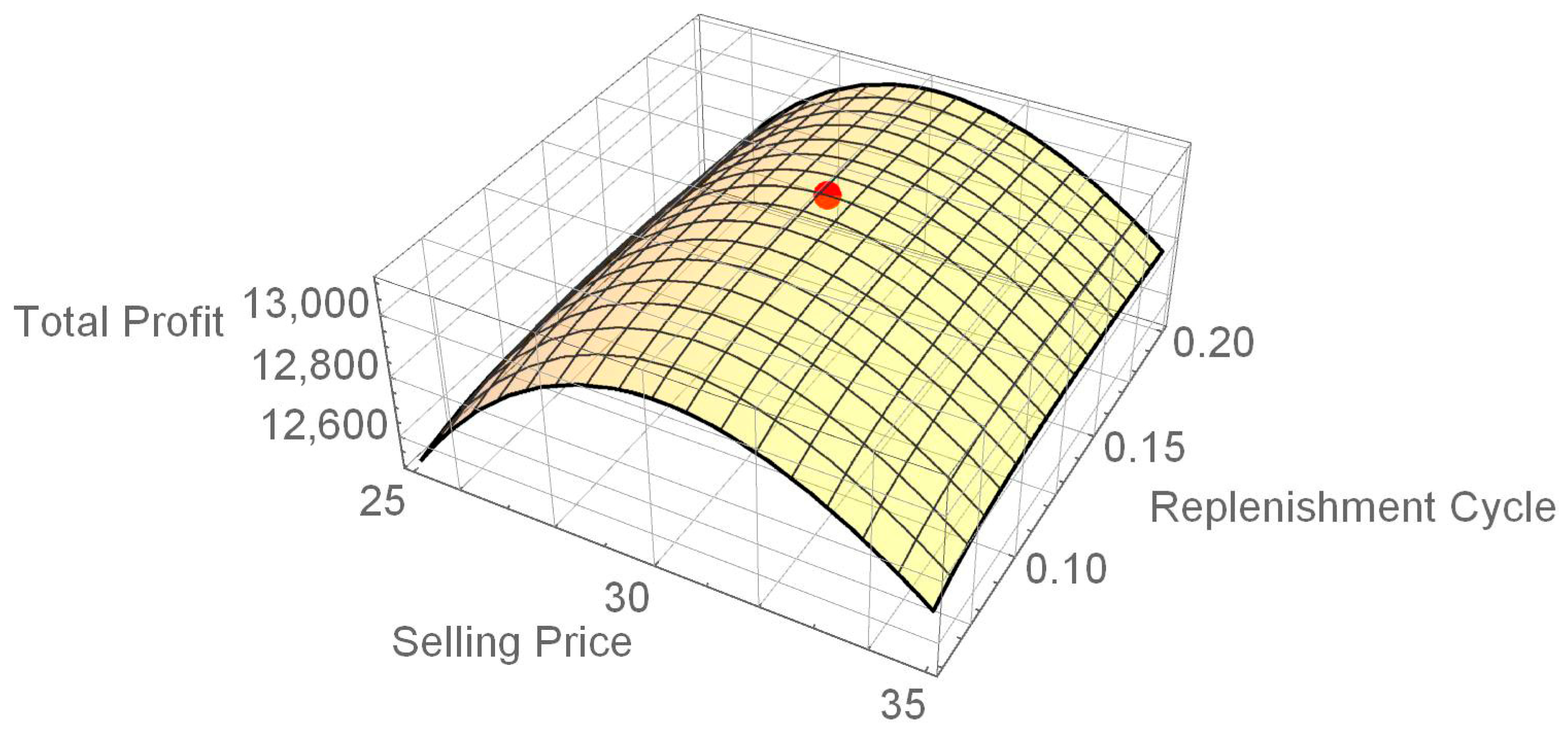
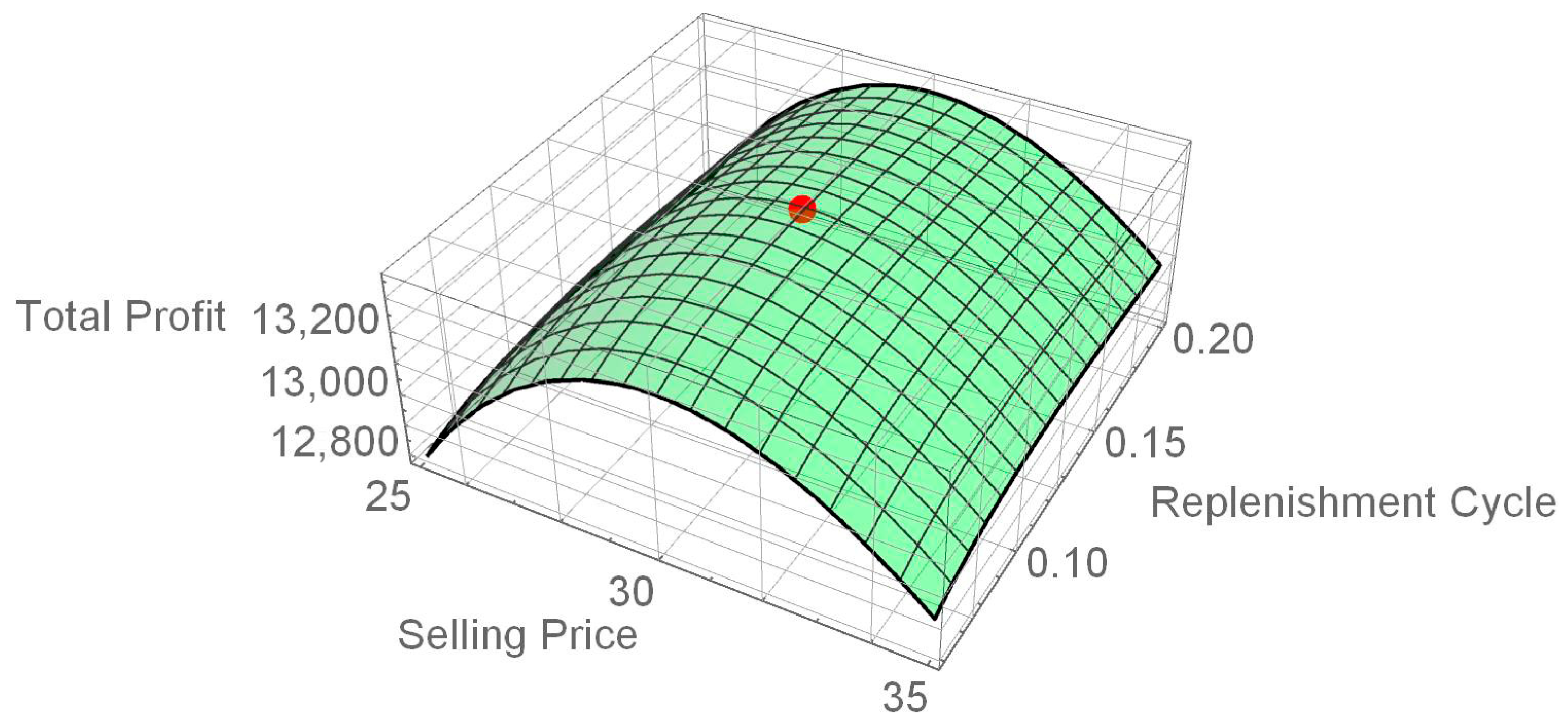
Thus, we know that ${TP}^{*}\left(p^{*},T^{*}\right)=max \left\{ 0, \mathrm{13,105.3}, 0\right\}=\mathrm{13,105.3}={TP}_{21}(p_{21},T_{21})$, and ${Model}_{21}$ is adopted. The optimal selling price $p^{*}=p_{21}=30.149$, the optimal replenishment cycle time ${T^{*}=T}_{21}=0.138803$, the optimal order quantity ${Q^{*}=Q}_{21}=92.61$ and the optimal discounted annual total profit $T{P}^{*}(p^{*}, T^{*})=\mathrm{13,105.3}$. The following expression represents the determinant of the Hessian matrix of ${TP}_{21}(p^{*},T^{*})$ at $\left(p^{*},T^{*}\right)$:

$$\left|\begin{array}{cc}-33.12& 32.98\\ 32.98& -\mathrm{13,427.85}\end{array}\right|=4.43642\times {10}^5 > 0.$$

It is evident from this equation that ${TP}_{21}(p^{*},T^{*})$ is maximized at $\left(p^{*},T^{*}\right)=(30.149,0.138803)$. The graph of ${TP}_{21}(p^{*},T^{*})$ is shown in Figure 6. The graph exhibits concaves at both $p$ and $T$. In this situation, ${Model}_{21}$ is optimal. As the optimal order quantity is greater than the predetermined quantity yet smaller than the warehouse capacity, the retailer benefits from the supplier’s trade credit and avoids the need for external storage rental.

• Situation 2: $0\le M<N$ and $Q_d\ge W$

Set $M=1/12$ years, $N=1/6$ years, $Q_d=150$, and $W=100$. By Appendix A, we have some results presented in

Table 4. The solutions for Situation 2.

Model [Constraints]	${\mathit{Q}}_{\mathit{i}\mathit{j}}$	${\mathit{p}}_{\mathit{i}\mathit{j}}$	${\mathit{T}}_{\mathit{i}\mathit{j}}$	${\mathit{T}\mathit{P}}_{\mathit{i}\mathit{j}}$
${Model}_{11}$ [$Q_{11}<Q_d$, $Q_{11}\le W$]	$Q_{11}=92.94<150$ $Q_{11}=92.94<100$	$p_{11}=30.216$	$T_{11}=0.139759$	${TP}_{11}=\mathrm{13,054.6}$
${Model}_{12}$ $[Q_{12}<Q_d$, $Q_{12}>W$]	$Q_{12}=111.96<150$ $Q_{12}=111.96>100$	$p_{12}=30.166$	$T_{12}=0.167809$	${\mathit{T}\mathit{P}}_{\mathbf{12}}=\mathbf{13,056.1}$
${Model}_{22}$ [$Q_{22}\ge Q_d$, $Q_{22}>W$]	$Q_{22}=113.39\ngeqq 150$ $Q_{22}=113.39>100$	$p_{22}=30.100$	$T_{22}=0.169379$	${TP}_{22}=0$

.

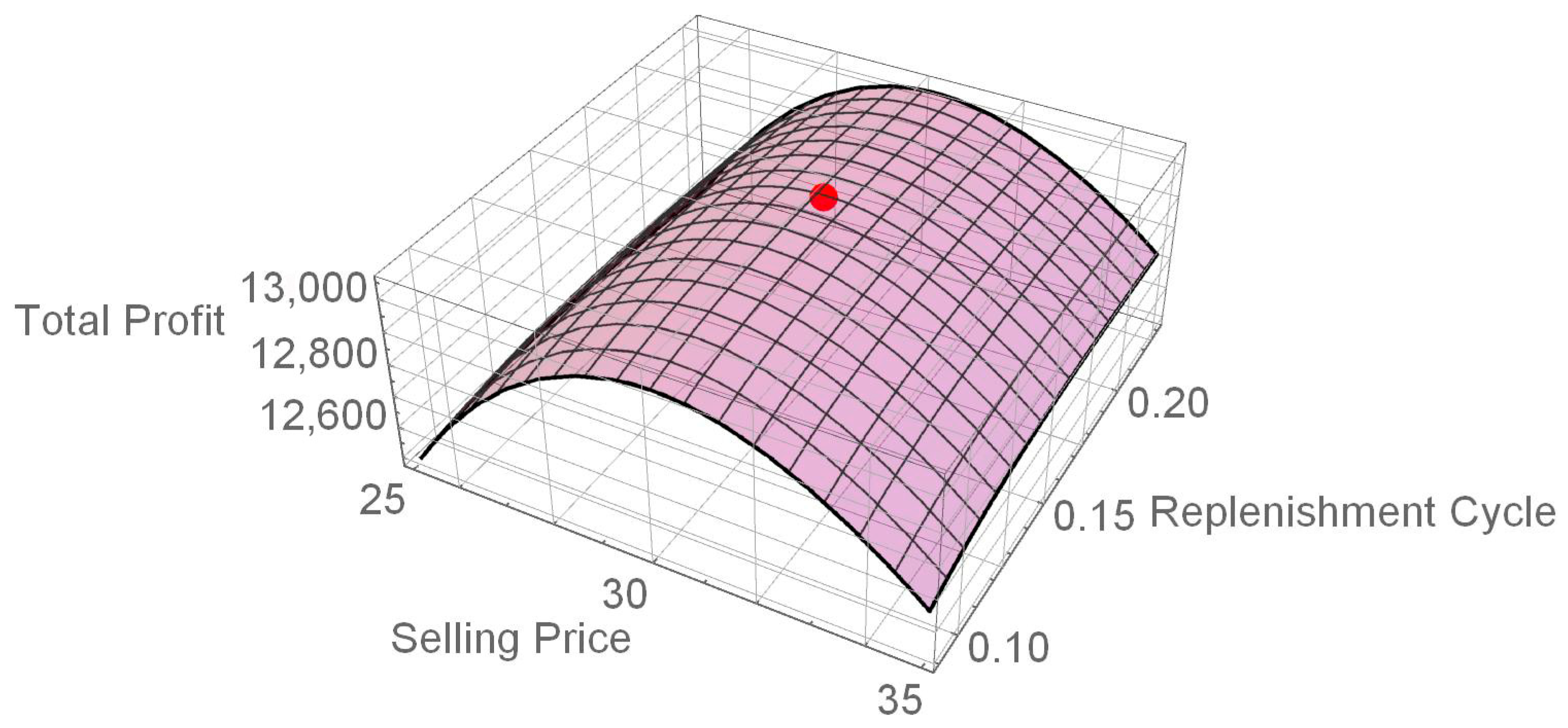
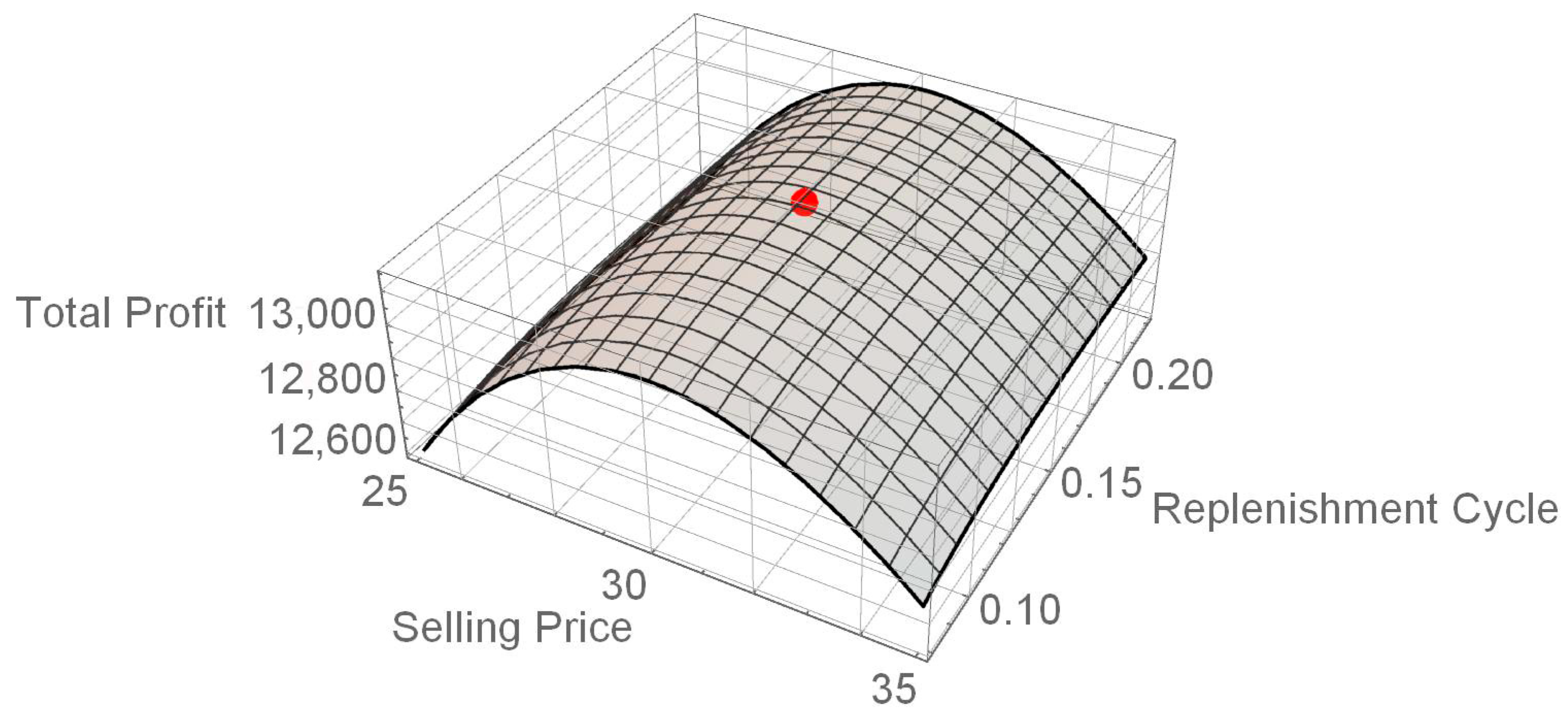
Thus, we know that ${TP}^{*}\left(p^{*},T^{*}\right)=max\left\{ \mathrm{13,054.6}, \mathrm{13,056.1}, 0\right\}=\mathrm{13,056.1}={TP}_{12}(p_{12},T_{12})$, and ${Model}_{12}$ is adopted. The optimal price $p^{*}=p_{12}=30.166$, the optimal replenishment time ${T^{*}=T}_{12}=0.167809$, the optimal order quantity ${Q^{*}=Q}_{12}=111.96$ and the optimal discounted annual total profit $T{P}^{*}(p^{*}, T^{*})=\mathrm{13,056.1}$. The following expression represents the determinant of the Hessian matrix of ${TP}_{12}(p^{*},T^{*})$ at $\left(p^{*},T^{*}\right)$:

$$\left|\begin{array}{cc}-33.35& 54.11\\ 54.11& -\mathrm{12,637.98}\end{array}\right|=4.18548\times {10}^5 > 0.$$

This equation shows that ${TP}_{12}(p^{*},T^{*})$ attains its maximum value at $\left(p^{*},T^{*}\right)=(30.166,0.167809)$. The graph of ${TP}_{12}(p^{*},T^{*})$ is shown in Figure 7. The graph exhibits concaves at both $p$ and $T$. In this situation, ${Model}_{12}$ is optimal. Since the optimal order quantity is less than the predetermined order quantity and larger than the capacity of the owned warehouse, the retailer cannot obtain the delay in payment offered by the supplier and needs to rent a warehouse for storage.

• Situation 3: $M\ge N$ and $Q_d<W$

Set $M=1/3$ years, $N=1/12$ years, $Q_d=50$, and W = 150. Hence, $M-N=0.25$. Using Appendix A, we obtain some results presented in

Table 5. The solutions for Situation 3.

Model [Constraints]	${\mathit{Q}}_{\mathit{i}\mathit{j}}$	${\mathit{p}}_{\mathit{i}\mathit{j}}$	${\mathit{T}}_{\mathit{i}\mathit{j}}$	${\mathit{T}\mathit{P}}_{\mathit{i}\mathit{j}}$
${Model}_{31}$ [$Q_{31}\ge Q_d$, $Q_{31}\le W$, $T_{31}\ge M-N$]	$Q_{31}=168.37>50$ $Q_{31}=168.37\nleqq 150$	$p_{31}=30.029$	$T_{31}=0.25$ $T_{31}=M-N$	${TP}_{31}=0$
${Model}_{32}$ [$Q_{32}\ge Q_d$, $Q_{32}>W$, $T_{32}\ge M-N$]	$Q_{32}=169.35>50$ $Q_{32}=169.35>150$	$p_{32}=29.913$	$T_{32}=0.25$ $T_{32}=M-N$	${TP}_{32}=\mathrm{13,323.8}$
${Model}_{41}$ [$Q_{41}\ge Q_d$, $Q_{41}\le W$, $T_{41}<M-N$]	$Q_{41}=86.87>50$ $Q_{41}=86.87<150$	$p_{41}=29.962$	$T_{41}=0.129025$ $T_{41}<M-N$	${\mathit{T}\mathit{P}}_{\mathbf{41}}=\mathbf{13,361.0}$
${Model}_{42}$ [$Q_{42}\ge Q_d$, $Q_{42}>W$, $T_{42}<M-N$]	$Q_{42}=124.50>50$ $Q_{42}=124.50\ngtr 150$	$p_{42}=29.840$	$T_{42}=0.183495$ $T_{42}<M-N$	${TP}_{42}=0$

.

Thus, we know that ${TP}^{*}\left(p^{*},T^{*}\right)=max\{ 0, \mathrm{13,323.8}, \mathrm{13,361.0}, 0\}=\mathrm{13,361.0}={TP}_{41}(p_{41},T_{41})$, and ${Model}_{41}$ is adopted. The optimal price $p^{*}=p_{41}=29.962$, the optimal replenishment time ${T^{*}=T}_{41}=0.129025$, the optimal order quantity ${Q^{*}=Q}_{41}=86.87$ and the optimal discounted annual total profit $T{P}^{*}(p^{*}, T^{*})=\mathrm{13,361.0}$. The following expression represents the determinant of the Hessian matrix of ${TP}_{41}(p^{*},T^{*})$ at $\left(p^{*},T^{*}\right)$:

$$\left|\begin{array}{cc}-33.79& 26.72\\ 26.72& -\mathrm{18,696.99}\end{array}\right|=6.31057\times {10}^5 > 0.$$

The results indicate that ${TP}_{41}(p,T)$ reaches its maximum at $\left(p^{*},T^{*}\right)=(29.962,0.129025)$. The graph of ${TP}_{41}(p^{*},T^{*})$ is shown in Figure 8. The graph exhibits concaves at both $p$ and $T$. In this situation, ${Model}_{41}$ is optimal. Because the optimal order quantity exceeds the predetermined order quantity but remains within the capacity of the retailer’s warehouse, the retailer can take advantage of the supplier’s delay in payment without renting additional storage.

• Situation 4: $M\ge N$ and $Q_d\ge W$

Set $M=1/10$ years, $N=1/12$ years, $Q_d=100$, and $W=75$. We know $M-N=0.0167$. Using Appendix A, we yield some results presented in

Table 6. The solutions for Situation 4.

Model [Constraints]	${\mathit{Q}}_{\mathit{i}\mathit{j}}$	${\mathit{p}}_{\mathit{i}\mathit{j}}$	${\mathit{T}}_{\mathit{i}\mathit{j}}$	${\mathit{T}\mathit{P}}_{\mathit{i}\mathit{j}}$
${Model}_{32}$ [$Q_{32}\ge Q_d$, $Q_{32}>W$, $T_{32}\ge M-N$]	$Q_{32}=102.0>$100 $Q_{32}=102.0$> 75	$p_{32}=30.075$	$T_{32}=0.152252$ $T_{32}=M-N$	${\mathit{T}\mathit{P}}_{\mathbf{32}}=\mathbf{13,145.7}$
${Model}_{42}$ [$Q_{42}\ge Q_d$, $Q_{42}>W$, $T_{42}<M-N$]	$Q_{42}=11.43\ngeqq 100$ $Q_{42}=11.43\ngtr 75$	$p_{42}=29.519$	$T_{42}=0.016667$ $T_{42}\nless M-N$	${TP}_{42}=0$

.

Thus, we know that ${TP}^{*}\left(p^{*},T^{*}\right)=max\{ \mathrm{13,145.7}, 0\}=\mathrm{13,145.7}={TP}_{32}(p_{32},T_{32})$, and ${Model}_{32}$ is adopted. The optimal price $p^{*}=p_{32}=30.075$, the optimal replenishment time ${T^{*}=T}_{32}=0.152252$, the optimal order quantity ${Q^{*}=Q}_{32}=102.0$ and the optimal discounted annual total profit $T{P}^{*}(p^{*}, T^{*})=\mathrm{13,145.7}$. The following expression represents the determinant of the Hessian matrix ${TP}_{32}(p^{*},T^{*})$ at $\left(p^{*},T^{*}\right)$:

$$\left|\begin{array}{cc}-33.42& 47.36\\ 47.36& -\mathrm{12,718.95}\end{array}\right|=4.26640\times {10}^5 > 0$$

According to this equation, ${TP}_{32}(p^{*},T^{*})$ achieves its maximum at $\left(p^{*},T^{*}\right)=(30.075,0.152252)$. The graph of ${TP}_{32}(p^{*},T^{*})$ is shown in Figure 9. The graph exhibits concavity at both $p$ and $T$. In this situation, ${Model}_{32}$ is optimal. Given that the optimal order quantity exceeds the predetermined quantity and surpasses warehouse capacity, the retailer is eligible for the supplier’s permissible delay in payment and is required to rent additional storage.

Based on the numerical illustrations above, we know that

(1)

For Situation 1, as the upstream trade credit period M is less than the downstream trade credit period N, and the predetermined order quantity,${ Q}_d$, is less than the capacity of the owner’s warehouse W, then ${\mathit{M}\mathit{o}\mathit{d}\mathit{e}\mathit{l}}_{\mathbf{21}}$ is the optimal one.

(2)

For Situation 2, as the upstream trade credit period M is less than the downstream trade credit period N, and the predetermined order quantity,${ Q}_d$, is not less than the capacity of the owner’s warehouse W, then ${\mathit{M}\mathit{o}\mathit{d}\mathit{e}\mathit{l}}_{\mathbf{12}}$ is the optimal one.

(3)

For Situation 3, as the upstream trade credit period M is not less than the downstream trade credit period N, and the predetermined order quantity,${ Q}_d$, is less than the capacity of the owner’s warehouse W, then ${\mathit{M}\mathit{o}\mathit{d}\mathit{e}\mathit{l}}_{\mathbf{41}}$ is the optimal one.

(4)

For Situation 4, as the upstream trade credit period M is not less than the downstream trade credit period N, and the predetermined order quantity,${ Q}_d$, is not less than the capacity of the owner’s warehouse W, then ${\mathit{M}\mathit{o}\mathit{d}\mathit{e}\mathit{l}}_{\mathbf{32}}$ is the optimal one.

As a result, we organize the optimal solution for each situation in

Table 7. Summary of the optimal solution for Situations 1–4.

	Relation 1	$0\hspace{0.33em}\le \hspace{0.33em}\mathit{M}\hspace{0.33em}<\hspace{0.33em}\mathit{N}$	$\mathit{M}\hspace{0.33em}\ge \hspace{0.33em}\mathit{N}$
Relation 2
$Q_d<W$		[Situation 1] ${\mathit{M}\mathit{o}\mathit{d}\mathit{e}\mathit{l}}_{\mathbf{21}},{TP}_{21}=\mathrm{13,105.3}$ $p_{21}=30.149$, $T_{21}=0.1388$, $Q_{21}=92.61$ $[Q_{21}\ge Q_d=50,$ $Q_{21}\le W=150$]	[Situation 3] ${\mathit{M}\mathit{o}\mathit{d}\mathit{e}\mathit{l}}_{\mathbf{41}}, {TP}_{41}=\mathrm{13,361.0}$ $p_{41}=29.962$, $T_{41}=0.1290$, $Q_{41}=86.87$ $[Q_{41}\ge Q_d=50,$ $Q_{41}\le W=150$]
$Q_d\ge W$		[Situation 2] ${\mathit{M}\mathit{o}\mathit{d}\mathit{e}\mathit{l}}_{\mathbf{12}}$, ${TP}_{12}=\mathrm{13,056.1}$ $p_{12}=30.166$, $T_{12}=0.1678$, $Q_{12}=111.96$ $[Q_{12}<Q_d=150,$ $Q_{12}>W=100$]	[Situation 4] ${\mathit{M}\mathit{o}\mathit{d}\mathit{e}\mathit{l}}_{\mathbf{32}}$, ${TP}_{32}=\mathrm{13,145.7}$ $p_{32}=30.075$, $T_{32}=0.015225$, $Q_{32}=102.2$ $[Q_{32}\ge Q_d=100,$ $Q_{32}>W=75$]

.

7. Sensitivity Analysis

Table 7 identifies Situation 3 as the most profitable scenario. Accordingly, the parameter values from Situation 3 are used for evaluating the impact of input parameter variations on the optimal solution. The findings of this sensitivity analysis are presented in

Table 8. Analysis of Parameter Sensitivity.

	Decision	${\mathit{p}}^{\mathit{*}}$	${\mathit{T}}^{\mathit{*}}$	${\mathit{Q}}^{\mathit{*}}$	$\mathit{T}{\mathit{P}}^{\mathit{*}}$	Model
Parameter
$A=15$		29.949	0.111782	75.27	13,402.5	${Model}_{41}$
$A=20$		29.962	0.129025	86.87	13,361.0	${Model}_{41}$
$A=25$		29.974	0.144206	97.07	13,324.4	${Model}_{41}$
Trend		↗	↗	↗	↘
$h=0.45$		29.960	0.129929	87.49	13,363.2	${Model}_{41}$
$h=0.50$		29.962	0.129025	86.87	13,361.0	${Model}_{41}$
$h=0.55$		29.965	0.128140	86.26	13,358.9	${Model}_{41}$
Trend		↗	↘	↘	↘
$c=8$		27.975	0.126698	94.21	14,772.1	${Model}_{41}$
$c=10$		29.962	0.129025	86.87	13,361.0	${Model}_{41}$
$c=12$		31.951	0.131639	80.25	12,083.4	${Model}_{41}$
Trend		↗	↘	↘	↘
$\theta =0.04$		29.952	0.132789	89.34	13,369.8	${Model}_{41}$
$\theta =0.06$		29.962	0.129025	86.87	13,361.0	${Model}_{41}$
$\theta =0.08$		29.972	0.125556	84.59	13,352.4	${Model}_{41}$
Trend		↗	↘	↘	↘
$k=0.55$		29.962	0.129025	86.87	13,361.0	${Model}_{41}$
$k=0.60$		29.962	0.129025	86.87	13,361.0	${Model}_{41}$
$k=0.65$		29.962	0.129025	86.87	13,361.0	${Model}_{41}$
Trend		---	---	---	---
$I_p=0.06$		29.962	0.129025	86.87	13,361.0	${Model}_{41}$
$I_p=0.07$		29.962	0.129025	86.87	13,361.0	${Model}_{41}$
$I_p=0.08$		29.962	0.129025	86.87	13,361.0	${Model}_{41}$
Trend		---	---	---	---
$I_e=0.04$		29.988	0.134762	90.63	13,317.5	${Model}_{41}$
$I_e=0.05$		29.962	0.129025	86.87	13,361.0	${Model}_{41}$
$I_e=0.06$		29.937	0.123966	83.56	13,405.1	${Model}_{41}$
Trend		↘	↘	↘	↗
$\alpha =0.02$		29.971	0.128992	86.81	13,344.4	${Model}_{41}$
$\alpha =0.04$		29.962	0.129025	86.87	13,361.0	${Model}_{41}$
$\alpha =0.06$		29.954	0.129058	86.92	13,377.6	${Model}_{41}$
Trend		↘	↗	↗	↗
$r=0.03$		29.968	0.136675	92.01	13,379.0	${Model}_{41}$
$r=0.05$		29.962	0.129025	86.87	13,361.0	${Model}_{41}$
$r=0.07$		29.957	0.122562	82.52	13,343.9	${Model}_{41}$
Trend		↘	↘	↘	↘
$a=2000$		29.985	0.157922	70.86	8860.9	${Model}_{41}$
$a=3000$		29.962	0.129025	86.87	13,361.0	${Model}_{41}$
$a=4000$		29.949	0.111782	100.36	17,870.0	${Model}_{41}$
Trend		↘	↘	↗	↗
$b=0.03$		43.273	0.099859	82.04	27,351.7	${Model}_{41}$
$b=0.04$		34.951	0.115073	85.59	18,512.1	${Model}_{41}$
$b=0.05$		29.962	0.129025	86.87	13,361.0	${Model}_{41}$
$b=0.06$		26.640	0.142324	86.72	10,041.7	${Model}_{41}$
$b=0.07$		24.269	0.155332	85.63	7759.7	${Model}_{41}$
Trend		↘	↗	↗↘	↘
$Q_d=50$		29.962	0.129025	86.87	13,361.0	${Model}_{41}$
$Q_d=75$		29.962	0.129025	86.87	13,361.0	${Model}_{41}$
$Q_d=100$		29.913	0.25000	169.35	13,323.8	${Model}_{32}$
$Q_d=150$		29.913	0.25000	169.35	13,323.8	${Model}_{32}$
Trend		X	X	X	X
$W=75$		29.925	0.143412	96.78	13,369.1	${Model}_{42}$
$W=150$		29.962	0.129025	86.87	13,361.0	${Model}_{41}$
$W=225$		29.962	0.129025	86.87	13,361.0	${Model}_{41}$
Trend		X	X	X	X
$M=1/4$		30.000	0.166667	112.12	13,295.1	${Model}_{31}$
$M=1/3$		29.962	0.129025	86.87	13,361.0	${Model}_{41}$
$M=1/2$		29.882	0.129354	87.44	13,526.6	${Model}_{41}$
Trend		↘	X	X	↗
$N=1/18$		29.954	0.129058	86.92	13,377.6	${Model}_{41}$
$N=1/12$		29.962	0.129025	86.87	13,361.0	${Model}_{41}$
$N=1/6$		29.930	0.166667	112.52	13,380.6	${Model}_{31}$
Trend		X	X	X	X

(Note: *: optimal solution; ↗: increasing; ↘: decreasing; ---: no change; X: uncertainty).

.

The results in Table 8 offer the following managerial implications:

• As the ordering cost A increases, the optimal selling price $p^{*}$, replenishment time $T^{*}$, and order quantity $Q^{*}$ rise, while the retailer’s total profit $T{P}^{*}\left(p^{*},T^{*}\right)$ declines. This implies that although higher ordering costs lead retailers to raise prices, extend replenishment cycles, and enlarge order quantities, the outcome is ultimately unfavorable for the retailer.
• An increase in unit holding cost h in OW, purchasing cost c, or deterioration rate $\theta$ leads to a higher optimal selling price $p^{*}$ but lower replenishment time $T^{*}$, order quantity $Q^{*}$, and retailer’s total profit $T{P}^{*}\left(p^{*},T^{*}\right)$. Hence, when these costs or risks rise, retailers should respond by increasing the selling price.
• When ${Model}_{41}$ is applied, no interest is charged, the order quantity does not exceed the OW capacity, and the RW is excluded. Consequently, the optimal solutions ($p^{*},T^{*}$, $Q^{*} \mathrm{a}\mathrm{n}\mathrm{d} T{P}^{*}\left(p^{*},T^{*}\right)$) remain unaffected by variations in the unit holding cost $k$ of RW and the interest rate $I_p$.
• When the earned interest rate $I_e$ increases, retailers set a lower selling price $p^{*}$, shorten the replenishment time $T^{*}$ and reduce order quantity $Q^{*}$, yet achieve higher retailer’s total profit $T{P}^{*}\left(p^{*},T^{*}\right)$. This demonstrates that improving the earned interest rate is advantageous for profitability.
• As the immediate payment fraction $\alpha$ increases, the optimal replenishment time $T^{*}$, order quantity $Q^{*}$ and the retailer’s total profit $T{P}^{*}\left(p^{*},T^{*}\right)$ rise, whereas the optimal selling price $p^{*}$ declines. This indicates that price reduction is an appropriate response to a higher immediate payment fraction.
• A rise in the discount rate $r$ reduces the optimal selling price $p^{*},$ replenishment time $T^{*}$, and order quantity $Q^{*}$, leading to lower the retailer’s total profit $T{P}^{*}\left(p^{*},T^{*}\right)$. This demonstrates that a higher discount rate $r$ negatively affects the retailer’s profitability.
• When the demand rate coefficient a grows, retailers benefit from larger order quantities $Q^{*}$ and higher retailer’s total profit $T{P}^{*}\left(p^{*},T^{*}\right)$, but they must reduce the selling price $p^{*}$ and shorten the replenishment time $T^{*}$.
• When the selling price coefficient b becomes larger, the retailer extends replenishment time $T^{*}$ but faces a decline in both selling price $p^{*}$ and retailer’s total profit $T{P}^{*}\left(p^{*},T^{*}\right)$. Meanwhile, the order quantity responds non-monotonically, initially rising but then decreasing once b exceeds 0.05.
• As $Q_d$ increases, ${Model}_{32}$ is applied when the predetermined order quantity $Q_d$ exceeds 86.87; otherwise, ${Model}_{41}$ is adopted. Transitioning from ${Model}_{41}$ to ${Model}_{32}$, the optimal replenishment time $T^{*}$ and order quantity $Q^{*}$ increase, whereas the optimal selling price $p^{*}$ and retailer’s total profit $T{P}^{*}\left(p^{*},T^{*}\right)$ decline.
• As the own-warehouse capacity W grows, the selection of the model depends on the order quantity Q: ${Model}_{42}$ is applied when it exceeds 86.87, otherwise ${Model}_{41}$ is used. Moving from ${Model}_{42}$ to ${Model}_{41}$, the optimal selling price $p^{*}$ rises, while the replenishment time $T^{*}$, order quantity $Q^{*}$, and retailer’s total profit $T{P}^{*}\left(p^{*},T^{*}\right)$ decrease, highlighting the trade-offs associated with warehouse capacity and model selection.
• A longer upstream trade credit period $M$ increases the retailer’s total profit $T{P}^{*}\left(p^{*},T^{*}\right)$ while lowering the selling price $p^{*}$. When $M=1/4$, then ${Model}_{31}$ is adopted; otherwise, ${Model}_{41}$ applies. For ${Model}_{41}$, an increase in $M$ leads to higher optimal replenishment time $T^{*}$ and order quantity $Q^{*}$
• If downstream trade credit period $N=1/6$, then ${Model}_{31}$ is chosen, otherwise, ${Model}_{41}$ is applied. Under ${Model}_{41}$, an increase in $N$ leads to a higher optimal selling price $p^{*}$ but lower optimal replenishment time $T^{*}$, order quantity $Q^{*}$ and retailer’s total profit $T{P}^{*}\left(p^{*},T^{*}\right)$.

8. Conclusions

In summary, this study develops an integrated supplier–retailer–customer chain model that limits to the given five conditions: (1) incorporates price-dependent demand, (2) includes a rented warehouse for limited storage, (3) considers partial trade credit, (4) links two-level trade credit terms to order quantity, and (5) evaluates financial performance on a present-value basis. The research establishes an optimal pricing framework for deteriorating goods with limited storage capacity (one or two warehouses), integrating downstream partial trade credit based on order quantity and discounted cash flow analysis. The supplier allows payment delays linked to order quantity, while the retailer provides partial trade credit to customers. The numerical results of the models have provided practical implications and demonstrated the model’s applicability in analyzing the effects of these supply chain mechanisms as follows.

• Higher ordering costs, unit holding costs, unit purchasing costs, and deterioration rates lead to an increase in the selling price, while simultaneously reducing the retailer’s total profit.
• An increase in the fraction of immediate payment, along with higher interest rates and demand rate coefficient, encourages a lower selling price, resulting in enhanced total profit for the retailer.
• Larger selling price coefficients and higher discount rates drive down the selling price and diminish the retailer’s total profit, highlighting the adverse effects of these factors on profitability.

As a result, a succinct highlight of the main contribution is presented. That is, a combination of a longer upstream trade credit period, a shorter downstream trade credit period, a smaller predetermined order quantity, and a larger warehouse capacity yields the highest total profit for the retailer, indicating the most advantageous operational condition.

The model can be extended in multiple directions. For instance, the payment scheme could be modified to an advance cash credit type. Additionally, the demand rate may be influenced by factors such as advertising, product quality, credit period, or be stochastic. Moreover, considering the inventory system for multi-item products, adding environmental sustainability constraints, or behavioral trade credit terms. Incorporating these factors, the demand function can be generalized as a joint function of price and advertising, quality, or credit period, thereby enhancing the model’s applicability.

References

1. Yang, H.L. An optimal replenishment cycle and order quantity inventory model for deteriorating items with fluctuating demand. Supply Chain Anal. 2023, 3, 10021. [Google Scholar] [CrossRef]
2. Alfares, H.K.; Ghaithan, A.M. Inventory and pricing model with price-dependent demand, time-varying holding cost, and quantity discounts. Comput. Ind. Eng. 2016, 94, 170–177. [Google Scholar] [CrossRef]
3. Feng, L.; Chan, Y.L.; Cárdenas-Barrón, L.E. Pricing and lot-sizing policies for perishable goods when the demand depends on selling price, displayed stocks, and expiration date. Int. J. Prod. Econ. 2017, 185, 11–20. [Google Scholar] [CrossRef]
4. Giri, B.C.; Bhattacharjee, R.; Maiti, T. Optimal payment time in a two-echelon supply chain with price-dependent demand under trade credit financing. Int. J. Syst. Sci. Oper. Logist. 2018, 5, 374–392. [Google Scholar] [CrossRef]
5. Rameswari, M.; Uthayakumar, R. An integrated inventory model for deteriorating items with price-dependent demand under two-level trade credit policy. Int. J. Syst. Sci. Oper. Logist. 2018, 5, 253–267. [Google Scholar] [CrossRef]
6. Li, R.; Teng, J.T.; Zheng, Y. Optimal credit term, order quantity and pricing policies for perishable products when demand depends on price, expiration date, and credit period. Ann. Oper. Res. 2019, 280, 377–405. [Google Scholar] [CrossRef]
7. Giri, B.C.; Masanta, M. Developing a closed-loop supply chain model with price and quality dependent demand and learning in production in a stochastic environment. Int. J. Syst. Sci. Oper. Logist. 2020, 7, 147–163. [Google Scholar] [CrossRef]
8. Li, R.; Teng, J.T.; Chang, C.T. Lot-sizing and pricing decisions for perishable products under three-echelon supply chains when demand depends on price and stock-age. Ann. Oper. Res. 2021, 307, 303–328. [Google Scholar] [CrossRef]
9. Feng, L.; Wang, W.C.; Teng, J.T.; Cárdenas-Barrón, L.E. Pricing and lot-sizing decision for fresh goods when demand depends on unit price, displaying stocks and product age under generalized payments. Eur. J. Oper. Res. 2022, 296, 940–952. [Google Scholar] [CrossRef]
10. Taleizadeh, A.A.; Aliabadi, L.; Thaichon, P. A sustainable inventory system with price-sensitive demand and carbon emissions under partial trade credit and partial backlogging. Oper. Res. 2022, 22, 4471–4516. [Google Scholar]
11. Yang, Y.; Liu, J. Price timing financing strategies for a capital-constrained supply chain with price-dependent stochastic demand. Int. J. Prod. Econ. 2023, 261, 108885. [Google Scholar] [CrossRef]
12. Das, S.C.; Zidan, A.M.; Manna, A.K.; Shaikh, A.A.; Bhunia, A.K. An application of preservation technology in inventory control system with price dependent demand and partial backlogging. Alex. Eng. J. 2020, 59, 1359–1369. [Google Scholar] [CrossRef]
13. Tayal, S.; Singh, S.R.; Katariya, C.; Handa, N. An inventory model with quantity dependent trade credit for stock and price dependent demand, variable holding cost and partial backlogging. Reliab. Theory Appl. 2021, 16, 225–240. [Google Scholar]
14. Bai, Y.; Li, H.; Gu, M. Advance selling policies with stochastic consumer valuations and advertising effects: Dynamic pricing and inventory decisions. Int. J. Prod. Econ. 2024, 277, 109401. [Google Scholar] [CrossRef]
15. Kausar, A.; Hasan, A.; Maheshwari, S.; Gautam, P.; Jaggi, C.K. Sustainable production model with advertisement and market price dependent demand under salvage option for defectives. Opsearch 2024, 61, 315–333. [Google Scholar] [CrossRef]
16. Pal, D.; Manna, A.K.; Ali, I.; Roy, P.; Shaikh, A.A. A two-warehouse inventory model with credit policy and inflation effect. Decis. Anal. J. 2024, 10, 100406. [Google Scholar] [CrossRef]
17. Lin, X.B.; Yu, J.C.P.; Chen, J.M. Optimizing a Sustainable Inventory Model Under Limited Recovery Rates and Demand Sensitivity to Price, Carbon Emissions, and Stock Conditions. Mathematics 2025, 13, 2916. [Google Scholar] [CrossRef]
18. Liu, L.; Li, X.; Zhu, S.; Wang, M. Retail Service, Pricing, and Channel Selection Strategies for Fashion Products in a Two-Stage Decision Model. Mathematics 2025, 13, 2575. [Google Scholar] [CrossRef]
19. Sharma, M.; Mittal, M.; Agarwal, D.; Dhanda, A.; Guchhait, R.; Sarkar, M. Optimal inventory and pricing strategies for integrated supply chains of growing items under carbon emission policies. Mathematics 2025, 13, 1567. [Google Scholar] [CrossRef]
20. Lin, F.; Jia, T.; Wu, F.; Yang, Z. Impacts of two-stage deterioration on an integrated inventory model under trade credit and variable capacity utilization. Eur. J. Oper. Res. 2019, 272, 219–234. [Google Scholar] [CrossRef]
21. Shekarabi, S.A.H.; Gharaei, A.; Karimi, M. Modelling and optimal lot-sizing of integrated multi-level multi-wholesaler supply chains under the shortages and limited warehouse space: Generalized outer approximation. Int. J. Syst. Sci. Oper. Logist. 2019, 6, 237–257. [Google Scholar] [CrossRef]
22. Yen, G.F.; Lin, S.D.; Lee, A.K. Optimal economic production quantity policies considering the holding cost of deteriorating raw materials under two-level trade credit and limited storage capacity. Open Access Libr. J. 2019, 6, e5140. [Google Scholar] [CrossRef]
23. Yang, H.L. Retailer’s ordering policy for demand depending on expiration date with limited storage capacity under supplier credits linked to order quantity and discounted cash flow. Int. J. Syst. Sci. Oper. Logist. 2021, 8, 136–153. [Google Scholar] [CrossRef]
24. Duary, A.; Das, S.; Arif, M.G.; Abualnaja, K.M.; Khan, M.A.A.; Zakarya, M.; Shaikh, A.A. Advance and delay in payments with the price-discount inventory model for deteriorating items under capacity constraint and partially backlogged shortages. Alex. Eng. J. 2022, 61, 1735–1745. [Google Scholar] [CrossRef]
25. Sicilia, J.; San-José, L.A.; Alcaide-López-de-Pablo, D.; Abdul-Jalbar, B. Optimal policy for multi-item systems with stochastic demands, backlogged shortages and limited storage capacity. Appl. Math. Model. 2022, 108, 236–257. [Google Scholar] [CrossRef]
26. Ambroszkiewicz, S.; Bylka, S. Relatively optimal policies for stock management in a supply chain with option for inventory space limitation. Appl. Math. Model. 2023, 114, 291–317. [Google Scholar] [CrossRef]
27. Zhang, J.; Zhang, Y.; Liu, S.; Zou, L. Pricing decision of capacity-sharing supply Chain under information asymmetry. J. Ind. Manag. Optim. 2025, 21, 5808–5845. [Google Scholar] [CrossRef]
28. Huang, Y.F.; Hsu, K.H. An EOQ model under retailer partial trade credit policy in supply chain. Int. J. Prod. Econ. 2008, 112, 655–664. [Google Scholar] [CrossRef]
29. Thangam, A.; Uthayakumar, R. Optimal pricing and lot-sizing policy for a two-warehouse supply chain system with perishable items under partial trade credit financing. Oper. Res. 2010, 10, 133–161. [Google Scholar] [CrossRef]
30. Chen, S.C.; Teng, J.T.; Skouri, K. Economic production quantity model for deteriorating items with up-stream full trade credit and down-stream partial trade credit. Int. J. Prod. Econ. 2014, 155, 302–309. [Google Scholar] [CrossRef]
31. Wu, J.; Chan, Y.L. Lot-sizing policies for deteriorating items with expiration dates and partial trade credit to credit-risk customers. Int. J. Prod. Econ. 2014, 155, 292–301. [Google Scholar] [CrossRef]
32. Wu, J.; Al-khateeb, F.B.; Teng, J.T.; Cárdenas-Barrón, L.E. Inventory models for deteriorating items with maximum lifetime under downstream partial trade credits to credit-risk customers by discounted cash-flow analysis. Int. J. Prod. Econ. 2016, 171, 105–115. [Google Scholar] [CrossRef]
33. Shah, N.H.; Jani, M.Y.; Chaudhari, U. Optimal ordering policy for deteriorating items under down-stream trade credit dependent quadratic demand with full up-stream trade credit and partial down-stream trade credit. Int. J. Math. Oper. Res. 2018, 12, 378–396. [Google Scholar] [CrossRef]
34. Tiwari, S.; Cárdenas-Barrón, L.E.; Goh, M.; Shaikh, A.A. Joint pricing and inventory model for deteriorating items with expiration dates and partial backlogging under two-level partial trade credits in supply chain. Int. J. Prod. Econ. 2018, 200, 16–36. [Google Scholar] [CrossRef]
35. Giri, B.C.; Sharma, S. Optimising an integrated production-inventory system under cash discount and retailer partial trade credit policy. Int. J. Syst. Sci. Oper. Logist. 2019, 6, 99–118. [Google Scholar] [CrossRef]
36. Mahata, P.; Mahata, G.C.; De, S.K. An economic order quantity model under two-level partial trade credit for time varying deteriorating items. Int. J. Syst. Sci. Oper. Logist. 2020, 7, 1–17. [Google Scholar] [CrossRef]
37. Taleizadeh, A.A.; Tavassoli, S.; Bhattacharya, A. Inventory ordering policy for mixed sale of products under inspection policy, multiple prepayment, partial credit, payment linked to order quantity and full backordering. Ann. Oper. Res. 2020, 287, 403–437. [Google Scholar] [CrossRef]
38. Taleizadeh, A.A.; Pourmohammad-Zia, N.; Konstantaras, I. Partial linked-to-order delayed payment and life time effects on decaying items ordering. Oper. Res. 2021, 21, 2077–2099. [Google Scholar] [CrossRef]
39. Chang, C.T.; Cheng, M.C.; Ouyang, L.Y. Deteriorating inventory model with advance-cash-credit payment schemes and partial backlogging. Soft Comput. 2025, 29, 2279–2295. [Google Scholar] [CrossRef]
40. Das, S.; Khan, M.A.A.; Mahmoud, E.E.; Abdel-Aty, A.H.; Abualnaja, K.M.; Shaikh, A.A. A production inventory model with partial trade credit policy and reliability. Alex. Eng. J. 2021, 60, 1325–1338. [Google Scholar] [CrossRef]
41. Xu, S.; Fang, L. Partial credit guarantee and trade credit in an emission-dependent supply chain with capital constraint. Transp. Res. Part E Logist. Transp. Rev. 2020, 135, 101859. [Google Scholar] [CrossRef]
42. Zou, X.; Tian, B. Retailer’s optimal ordering and payment strategy under two-level and flexible two-part trade credit policy. Comput. Ind. Eng. 2020, 142, 106317. [Google Scholar] [CrossRef]
43. Dai, Z.; Wang, Y. A production and inventory model for deteriorating items with two-level partial trade credit and stochastic demand in a supply chain. Kybernetes 2023, 52, 4846–4875. [Google Scholar] [CrossRef]
44. Moradi, S.; Gholamian, M.R.; Sepehri, A. An inventory model for imperfect quality items considering learning effects and partial trade credit policy. Opsearch 2023, 60, 276–325. [Google Scholar] [CrossRef]
45. Choudhury, M.; Mahata, G.C. Non-instantaneous deteriorating items inventory models with fixed lifetime products under hybrid partial prepayment and trade credit in supply chain. J. Ind. Manag. Optim. 2024, 20, 221–259. [Google Scholar] [CrossRef]
46. Ouyang, L.Y.; Teng, J.T.; Goyal, S.K.; Yang, C.T. An economic order quantity for deteriorating items with partially permissible delay in payments linked to order quantity. Eur. J. Oper. Res. 2009, 194, 418–431. [Google Scholar] [CrossRef]
47. Kreng, V.B.; Tan, S.J. The optimal replenishment decision under two levels of trade credit policy depending on the order quantity. Expert Syst. Appl. 2010, 37, 5514–5522. [Google Scholar] [CrossRef]
48. Shah, N.H.; Cárdenas-Barrón, L.E. Retailer’s decision for ordering and credit policies for deteriorating items when a supplier offers order-linked credit or cash discount. Appl. Math. Comput. 2015, 259, 569–578. [Google Scholar] [CrossRef]
49. Tiwari, S.; Cárdenas-Barrón, L.E.; Shaikh, A.A.; Goh, M. Retailer’s optimal ordering policy for deteriorating items under order-size dependent trade credit and complete backlogging. Comput. Ind. Eng. 2020, 139, 105559. [Google Scholar] [CrossRef]
50. Tsao, Y.C.; Fauziah, H.A.; Vu, T.L.; Masruroh, N.A. Optimal pricing, ordering, and credit period policies for deteriorating products under order-linked trade credit. J. Ind. Manag. Optim. 2022, 18, 4151–4182. [Google Scholar] [CrossRef]
51. Chung, K.J.; Liao, J.J.; Srivastava, H.M.; Lee, S.F.; Lin, S.D. The EOQ model for deteriorating items with a conditional trade credit linked to order quantity in a supply chain system. Mathematics 2021, 9, 2311. [Google Scholar] [CrossRef]
52. Chen, S.C.; Teng, J.T. Inventory and credit decisions for time-varying deteriorating items with up-stream and down-stream trade credit financing by discounted cash flow analysis. Eur. J. Oper. Res. 2015, 243, 566–575. [Google Scholar] [CrossRef]
53. Yang, H.L.; Chang, C.T.; Tseng, Y.T. Optimal replenishment strategy for a high-tech product demand with non-instantaneous deterioration under an advance-cash-credit payment scheme by a discounted cash-flow analysis. Mathematics 2024, 12, 3160. [Google Scholar] [CrossRef]
54. Chang, C.T.; Tseng, Y.T. The impacts of payment schemes and carbon emission policies on replenishment and pricing decisions for perishable products in a supply chain. Mathematics 2024, 12, 1033. [Google Scholar] [CrossRef]
55. Sutjipto, E.; Setiawan, W.; Ghozali, I. Determination of intrinsic value: Dividend discount model and discounted cash flow methods in Indonesia Stock Exchange. Eddy Sutjipto, Wawan Setiawan and Imam Ghozali, Determination of Intrinsic Value: Dividend Discount Model and Discounted Cash Flow Methods in Indonesia Stock Exchange. Int. J. Manag. 2020, 11, 1842–1852. [Google Scholar]
56. Viswanath, J.; Thilagavathi, R.; Karthik, K.; Mahdal, M. A study of a two storage single product inventory system with ramp type demand, n-phase prepayment and purchase for exigency. Mathematics 2023, 11, 1728. [Google Scholar] [CrossRef]
57. Pathak, K.; Yadav, A.S.; Agarwal, P. Optimizing Two-Warehouse Inventory for Shelf-Life Stock with Time-Varying Bi-Quadratic Demand Under Shortages and Inflation. Math. Model. Eng. Probl. 2024, 11, 446–456. [Google Scholar] [CrossRef]
58. Tsao, Y.C.; Pantisoontorn, A.; Vu, T.L.; Chen, T.H. Optimal production and predictive maintenance decisions for deteriorated products under advance-cash-credit payments. Int. J. Prod. Econ. 2024, 269, 109132. [Google Scholar] [CrossRef]
Figure 1. Graphical representation of the inventory Model, if Q > W .
Mathematics 14 00163 g001
Figure 2. (a) Graphical representation for cash payment, if T < T d . (b) Graphical representation for credit payment, if T < T d .
Mathematics 14 00163 g002
Figure 3. (a) Graphical representation for cash payment, if T T d and M < N . (b) Graphical representation for credit payment, if T T d and M < N .
Mathematics 14 00163 g003
Figure 4. (a) Graphical representation for cash payment, if T T d , 0 < N M and M T + N . (b) Graphical representation for credit payment, if T T d , 0 < N M and M T + N .
Mathematics 14 00163 g004
Figure 5. (a) Graphical representation for cash payment, if T T d , 0 < N M and M > T + N . (b) Graphical representation for credit payment, if T T d , 0 < N M and M > T + N .
Mathematics 14 00163 g005aMathematics 14 00163 g005b
Figure 6. The graph of T P 21 ( p * , T * ) .
Mathematics 14 00163 g006
Figure 7. The graph of T P 12 ( p * , T * ) .
Mathematics 14 00163 g007
Figure 8. The graph of T P 41 ( p * , T * ) .
Mathematics 14 00163 g008
Figure 9. The graph of T P 32 ( p * , T * ) .
Mathematics 14 00163 g009