Article

An Age-Distributed Immuno-Epidemiological Model with Information-Based Vaccination Decision

1
Department of Mathematics and Statistics, Indian Institute of Technology Kanpur, Kanpur 208016, India
2
Institut Camille Jordan, UMR 5208 CNRS, University Lyon 1, 69622 Villeurbanne, France
3
Institute of Mathematics, Peoples Friendship University of Russia (RUDN University), 6 Miklukho-Maklaya St., Moscow 117198, Russia
*
Author to whom correspondence should be addressed.
Mathematics 2026, 14(1), 162; https://doi.org/10.3390/math14010162
Submission received: 16 November 2025 / Revised: 23 December 2025 / Accepted: 24 December 2025 / Published: 31 December 2025
(This article belongs to the Special Issue Models in Population Dynamics, Ecology and Evolution)

Abstract

An age-distributed immuno-epidemiological model with information-based vaccination proposed in this work represents a system of integro-differential equations with compartments for the numbers of susceptible individuals, infected individuals, vaccinated individuals, and recovered individuals. This model describes the influence of vaccination decisions on epidemic progression in different age groups. In a particular case of the model without age distribution, we determine the basic reproduction number and the final size of epidemic, that is, the limiting number of susceptible individuals at asymptotically large time. Moreover, we study the existence and uniqueness of a positive solution for the age-structured model. Numerical simulations show that the information-based vaccination acceptance can significantly influence the epidemic progression. Though the initial stage of epidemic progression is the same for all memory kernels, as the epidemic progresses and more information about the disease becomes available, further epidemic progression strongly depends on the memory effect. A short-range memory kernel appears to be more effective in restraining the epidemic outbreaks because it allows for more responsive and adaptive vaccination decisions based on the most recent information about the disease. Additionally, the simulation results suggest that relying on either a responsive vaccination approach or a highly effective vaccine alone may be insufficient to significantly reduce the epidemic size and prevent large outbreaks. Both factors are necessary to achieve substantial epidemic control. Moreover, the impacts of the age-dependent initial susceptible population and the age-dependent memory kernel are studied through numerical simulation of the age-dependent model.

1. Introduction

Modern epidemiology covers a wide spectrum of mathematical models in epidemiology, mainly based upon the ordinary differential equations and partial differential equations, integro-differential equations, individual-based methods, and some other modeling tools. The ordinary differential equation epidemic models were introduced by D. Bernoulli in the 18th century to study the smallpox epidemic [1]. Another remarkable step in the development of mathematical epidemiology is the works by W. O. Kermack and A. G. McKendrick [2,3,4], where the foundation of modern developments in mathematical epidemiology was established. These approaches were further developed in various multi-compartmental models (see, e.g., [5,6,7,8]), agent-based models [9,10], immuno-epidemic models [11,12,13,14], network models [15,16], multi-scale models [17,18], age-structured models [19,20,21,22,23,24], age of infection models [25,26], and data-driven models [27,28,29]. A substantial body of work has focused on analyzing SIR-type epidemic models exhibiting various bifurcation behaviors, including backward bifurcation [30], forward–backward bifurcation [31], transcritical bifurcation [32], and Hopf bifurcation [33,34]. Optimal control techniques have been applied to mitigate infection levels, incorporating multiple intervention strategies such as treatment, preventive measures, and vaccination [30,35,36]. Fractional-order epidemic models in biology have been developed to more accurately model the spread and control of infectious diseases [37]. In the context of COVID-19, a harmonic mean-type incidence rate is used to examine the dynamic behaviors [38] through fractional calculus analysis. In [39], the authors use a convex incidence rate and sensitivity analysis to study the progression of the infection. Stochastic modeling approaches are also implemented to study epidemic progression. The transmission probabilities can be modeled using a continuous-time Markov process [40]. Stochastic models combined with Monte Carlo simulations are used to study network-based epidemic models [41,42]. Recently, machine learning and deep learning techniques have also been widely employed to forecast the spread of COVID-19 [43]. Physics-Informed Neural Networks, where deep neural networks are coupled with physics-based models such as SIR-type models, are also used to predict epidemic progression [44,45].
One of the directions of these investigations concerns the influence of vaccination on epidemic progression. Vaccination is one of the most effective measures to restrain epidemic progression. However, the success of vaccination strategy depends on the available information about the epidemic and the risk of adverse events [46,47]. COVID-19 epidemic has provided numerous examples of uncoordinated behavioral responses to infection threats and control measures [48]. Vaccine hesitancy has currently been included by WHO among the most serious threats to global health [49].
Vaccine hesitancy arises from a range of factors such as misinformation, lack of trust in healthcare systems, safety concerns, and social or cultural influences [50]. Inconsistent messaging and the rapid spread of misinformation may lead to confusion and fear related to vaccination. Addressing vaccine hesitancy requires more than just making vaccines available: it demands clear, consistent communication, fostering public trust, and actively engaging with communities to address their concerns.
Behavioral epidemiology is an interdisciplinary field that seeks to understand how human behavior influences the spread of infectious diseases [46]. It combines traditional epidemiological models with theories and methods from behavioral sciences to better understand the complex social and psychological factors that contribute to the transmission of infectious diseases. By incorporating insights from multiple disciplines, behavioral epidemiology provides a more nuanced understanding of the influence of human behavior on the infectious disease transmission. This can inform the development of more effective public health interventions that take into account the social and psychological factors that influence people’s behavior [51,52].
Epidemic models with vaccination decisions based upon information were introduced in [46]. One of the possible developments of this theory consists in the introduction of age-distributed vaccination decision in the model. Different age groups may have different attitudes towards vaccination, and these attitudes may be influenced by various age-specific factors such as the severity of the disease, the perceived benefits and risks of vaccination, and the cost of vaccination. In the case of influenza, the  distribution of vaccinated people according to the age groups is analyzed in [53] (see Figure 1a). Recent studies of COVID-19 epidemic reveal that younger people are more hesitant about vaccination than older people [54,55,56,57] (see Figure 1b). This is clearly related to the age-distributed death rate for the SARS-CoV-2 infection. Numerous studies for different infectious diseases show that vaccination decisions vary between the age groups. Thus, it is very relevant to study the impact of age-specific vaccination decisions on the epidemic outbreaks.
In this work, we introduce and study an age-distributed epidemic model with information-based vaccination decisions.
The key contributions of this work are as follows:
  • Propose an age-distributed epidemic model with information-based vaccination decisions. This study continues the previous works on epidemic models that involve time-since-infection distributed recovery rates and death rates [11,26,58]. This approach allows us to take into account time-dependent recovery and death rates which give a more accurate understanding of epidemic progression than the conventional SIR models.
  • Establish the existence and uniqueness of a positive solution for the proposed age-distributed model.
  • For the age-independent version of the proposed model, derive the analytical expression of R 0 under different choices of recovery and death distributions and determine the bounds for the final size of the epidemic.
  • Conduct extensive numerical simulations to explore the effects of various parameters involved in information-based vaccination decisions, such as the impact of the memory kernel and the baseline probability of vaccination.
The paper is organized as follows. We propose the age-distributed model with information-based vaccination decisions in Section 2. In Appendix A, we prove the existence and uniqueness a of positive solution of the proposed model. Section 3 is devoted to the reduced model without age distribution for which we determine an analytical bound for the final size of epidemic depending on the information-based vaccination uptake. The influence of information-dependent vaccination uptake on the epidemic progression is illustrated with the help of numerical simulation in Section 4.

2. Model Formulation

In this section, we develop an age-distributed immuno-epidemiological model that incorporates the influence of viral load on the disease transmission rate. Our model is articulated in terms of the number of newly infected individuals, accounting for variable recovery and death rates as well as the age distribution of the population. Additionally, we integrate a vaccination rate influenced by information-dependent vaccination decisions.
Before formulating the model, it is important to clarify that demographic factors, such as natural birth and death rates, play a significant role in epidemic models that consider vertical transmission or that aim to examine epidemic progression over extended periods. However, our primary objective is to analyze the epidemic progression over a relatively short duration, where demographic changes are not sufficiently influential. Specifically, the rate of change from one age group to another is negligible over this short period. To illustrate, if we study a human epidemic with a time unit of ‘days’ over a period of a few months, the rate of natural death is approximately 1 / ( 365 × 100 ) days 1 0.000027 days 1 , which is negligible. Furthermore, vertical transmission is not addressed in this work. Consequently, we do not consider demographic factors like natural births and deaths in our model formulation.
Given this context, we adopt an age-distributed framework where the total population within each age group is assumed to remain constant. This simplification allows us to focus on the dynamic interactions between infection, recovery, and vaccination within a structured population without the added complexity of demographic changes.

2.1. Distributed Recovery and Death Rates

Let an individual’s age a vary between 0 and A M , where A M > 0 is the maximum possible age of an individual, and let J ( a , t ) be a non-negative function denoting the rate at which susceptible individuals of age a are newly infected at time t. Suppose that S ( a , t ) , I ( a , t ) , R ( a , t ) , and  D ( a , t ) represent the numbers of susceptible individuals, actively infected individuals, recovered individuals, and dead individuals of age a at time t. Then the total number of individuals of age a being infected during time 0 to t (i.e., 0 t J ( a , ζ ) d ζ ) can be written as follows [26]:
0 t J ( a , ζ ) d ζ = I ( a , t ) + R ( a , t ) + D ( a , t ) .
Here, time t = 0 refers to the beginning of the epidemic. We also suppose that for each age group a, the total population is constant for all time t > 0 , i.e., 
( S + I + R + D ) ( a , t ) = S 0 ( a ) ,
where S 0 ( a ) is the initial population size in the age group a. Note that S 0 ( a ) is assumed to be constant for all a because demographic factors are not considered in the model, as the study period is assumed to be significantly shorter than the maximum age A M . Using this assumption and differentiating (1) with respect to t, we obtain
S ( a , t ) t = J ( a , t ) .
Next, we suppose that the infection rate varies proportionally with the viral load in the population [59]. We let V ( a ) denote the viral load of an infected individual of age a at any time during their infectious period. Then, using (2), we get
J ( a , t ) = S ( a , t ) t = α ( a ) S ( a , t ) 0 A M V ( y ) I ( y , t ) d y ,
where the coefficient α ( a ) accounts for the age-distributed susceptibility rate. In the case of an age-independent infectivity rate, the last formula becomes similar to the conventional SIR model.
We let r ( a , ξ ) and d ( a , ξ ) denote, respectively, the recovery and death distributions for the infected individuals in the age group a depending on time post-infection ξ . Then, we obtain the governing equation for I ( a , t ) , R ( a , t ) and D ( a , t ) :
I ( a , t ) t = J ( a , t ) 0 t r ( a , t ζ ) J ( a , ζ ) d ζ 0 t d ( a , t ζ ) J ( a , ζ ) d ζ ,
R ( a , t ) t = 0 t r ( a , t ζ ) J ( a , ζ ) d ζ , D ( a , t ) t = 0 t d ( a , t ζ ) J ( a , ζ ) d ζ .
To set up the final model now we introduce the information-based vaccination in the following subsection.

2.2. Information-Based Vaccination

We let ρ ( a , t ) denote the proportion of vaccinated individuals of age a at time t. We assume that vaccinated individuals are completely protected from infection, a common assumption in many epidemic models with idealized vaccine efficacy. Since the model is designed to study epidemic progression over a relatively short time span, the assumption of permanent immunity within this period is well justified. Additionally, we assume that vaccination is administered only to the susceptible individuals, not to the infected individuals. Then, instead of Equations (2)–(4), we get the equations
S ( a , t ) t = α ( a ) S ( a , t ) ( 1 ϵ ρ ( a , t ) ) 0 A M V ( y ) I ( y , t ) d y ( J ( a , t ) ) ,
I ( a , t ) t = α ( a ) S ( a , t ) ( 1 ϵ ρ ( a , t ) ) 0 A M V ( y ) I ( y , t ) d y 0 t r ( a , t ζ ) J ( a , ζ ) d ζ
0 t d ( a , t ζ ) J ( a , ζ ) d ζ .
The governing equation for the age-specific vaccination rate is given by
ρ ( a , t ) t = P ( m ( I ( a , t ) ) ) ( 1 ρ ( a , t ) ) .
Here, ϵ denotes the vaccine effectiveness which lies between 0 and 1. A value of ϵ = 1 indicates a fully effective vaccine, while ϵ = 0 signifies complete vaccine failure. m ( a , t ) is an information index which summarizes the age-specific and time varying information on the present and past incidence of the infection along with its sequel [60], P ( m ) is a positive function that represents the probability of vaccine uptake which takes into account the vaccine hesitancy [60]. It can be considered as a monotonically increasing function of the information index m implying that better informed people are more inclined towards vaccination [60].
Hence, the age-distributed epidemic model with information-based vaccine uptake is given by Equations (5)–(8) with the initial conditions
S ( a , 0 ) = S 0 ( a ) , I ( a , 0 ) = I 0 ( a ) , R ( a , 0 ) = R 0 ( a ) ,
D ( a , 0 ) = D 0 ( a ) , ρ ( a , 0 ) = ρ 0 ( a ) .
Here, all the functions are continuous and non-negative for a [ 0 , A M ] .
Let us consider the following condition for the recovery and death rates:
ζ t 0 ( r ( a , ξ ζ ) + d ( a , ξ ζ ) ) d ξ 1
for any ζ and t 0 , t 0 > ζ and a. This is an epidemiologically justified condition: the left hand side represents the proportion of total recovery and death during the time ζ to t 0 , among the individuals who were infected at time ζ , and this proportion must be less than or equal to 1 (see [58] for further details). The descriptions along with dimensions of the variables and parameters in the model are summarized in Table 1. The detailed study of the existence and uniqueness of a positive solution is available in Appendix A.

3. Model Without Age Distribution

In this section, we consider a particular case of Models (5)–(8) with age-independent parameters. By aggregating the compartments over the entire age range and assuming age-independent parameters, the original age-distributed model is transformed into a more mathematically tractable form. This reduction simplifies the analysis and facilitates the derivation of analytical results. Set
S ^ ( t ) = 0 A M S ( a , t ) d a , I ^ ( t ) = 0 A M I ( a , t ) d a ,
R ^ ( t ) = 0 A M R ( a , t ) d a , D ^ ( t ) = 0 A M D ( a , t ) d a .
Let the information index be age-independent, i.e.,  m ^ ( t ) m ( I ^ ( t ) ) . Denote by ρ ^ ( t ) the proportion of people vaccinated at time t. Let P ^ ( m ) denote the age-independent information. Then, the equation of the vaccination compartment is given by
d ρ ^ ( t ) d t = P ( m ^ ) ( 1 ρ ^ ( t ) ) .
Assume α ( a ) , V ( a ) , r ( a , t ) , and d ( a , t ) are age-independent and set α ^ = α ( a ) , V ^ = V ( a ) , β ^ / N = α ^ V ^ , r ^ ( t ) = r ( a , t ) and d ^ ( t ) = d ( a , t ) , where N is the total population size. Now, integrating System (5)–(8) from 0 to A M with respect to a, we obtain the reduced system:
d S ^ ( t ) d t = β ^ N S ^ ( t ) ( 1 ϵ ρ ^ ( t ) ) I ^ ( t ) ( J ^ ( t ) ) ,
d I ^ ( t ) d t = β ^ N S ^ ( t ) ( 1 ϵ ρ ^ ( t ) ) I ^ ( t ) 0 t r ^ ( t ζ ) J ^ ( ζ ) d ζ 0 t d ^ ( t ζ ) J ^ ( ζ ) d ζ ,
d R ^ ( t ) d t = 0 t r ^ ( t ζ ) J ^ ( ζ ) d ζ ,
d D ^ ( t ) d t = 0 t d ^ ( t ζ ) J ^ ( ζ ) d ζ ,
d ρ ^ ( t ) d t = P ( m ^ ( t ) ) ( 1 ρ ^ ( t ) ) ,
with
S ^ ( 0 ) = S ^ 0 0 , I ^ ( 0 ) = I ^ 0 0 , R ^ ( 0 ) = R ^ 0 0 , D ^ ( 0 ) = D ^ 0 0 , ρ ^ ( 0 ) = ρ ^ 0 0 .
Here, β ^ signifies the average transmission rate in the population. This reduced model without age distribution (11)–(15) is simpler than the original age-distributed Model (5)–(8), but it still captures the effect of information-dependent behavior of vaccine uptake. In the next subsection, we find a bound for the final size of epidemic for this model.

3.1. Basic Reproduction Number

At the beginning of the epidemic S ^ ( t ) N , I ^ ( t ) e λ t and ρ ^ ( t ) = ρ ^ 0 . Then J ^ ( t ) β ^ ( 1 ϵ ρ ^ 0 ) e λ t . Putting these in Equation (12),
λ e λ t = β ^ ( 1 ϵ ρ ^ 0 ) e λ t β ^ ( 1 ϵ ρ ^ 0 ) 0 t ( r ^ ( t ζ ) + d ^ ( t ζ ) ) e λ ζ d ζ ,
which gives
λ = β ^ ( 1 ϵ ρ ^ 0 ) 1 0 t ( r ^ ( z ) + d ^ ( z ) ) e λ z d z .
Case I. Dirac delta function for recovery and death rates. Suppose the disease duration is τ , and the individuals J ^ ( t τ ) who were infected at time t τ recover or die at time t based on specific probabilities. This assumption leads to the following specific forms for functions r ^ ( t ) and d ^ ( t ) :
r ^ ( t ) = r 0 δ ( t τ ) , d ^ ( t ) = d 0 δ ( t τ ) ,
where r 0 , d 0 are positive constants with r 0 + d 0 = 1 and  δ is the Dirac delta-function. Then,
0 t ( r ^ ( z ) + d ^ ( z ) ) e λ z d z = e λ τ .
Then, Equation (16) reduces to
λ = β ^ ( 1 ϵ ρ ^ 0 ) 1 e λ τ .
Let H ( λ ) = β ^ ( 1 ϵ ρ ^ 0 ) 1 e λ τ . It is easy to observe that Equation (17) has a solution λ = 0 and a non-zero solution whose sign is determined by H ( 0 ) . Denote
R 0 = H ( 0 ) = β ^ ( 1 ϵ ρ ^ 0 ) τ .
Let R 0 > 1 . This implies, H ( 0 ) > 1 . It can be observed that H ( λ ) is an increasing function of λ and lim λ H ( λ ) = β ^ ( 1 ϵ ρ ^ 0 ) . Consequently, Equation (17) admits a positive solution, i.e., there exists λ + > 0 s.t. H ( λ + ) = λ + . If R 0 < 1 , i.e.,  H ( 0 ) < 1 , then
H ( λ ) = β ^ ( 1 ϵ ρ ^ 0 ) τ e λ τ < 1
for all λ 0 . This implies that equation H ( λ ) = λ has no positive solution.
Hence, the basic reproduction number is given by the following expression:
R 0 = β ^ ( 1 ϵ ρ ^ 0 ) τ .
If ρ ^ 0 = 0 , then the expression of R 0 is the same as that obtained for the delay model in our previous work [61].
  • Case II: Constant rate of recovery and death. If we assume the uniform distribution of recovery and death rate
r ^ ( t ) = r 0 , 0 t τ 0 , t > τ , d ^ ( t ) = d 0 , 0 t τ 0 , t > τ ,
where τ > 0 is disease duration, r 0 and d 0 are some constants, with  ( r 0 + d 0 ) τ = 1 . Then Equation (16) reduces to
λ = β ^ ( 1 ϵ ρ ^ 0 ) 1 ( r 0 + d 0 ) ( 1 e λ τ ) λ .
Let H ( λ ) = β ^ ( 1 ϵ ρ ^ 0 ) 1 ( r 0 + d 0 ) ( 1 e λ τ ) λ . Note that lim λ 0 H ( λ ) = β ^ ( 1 ϵ ρ ^ 0 ) ( 1 ( r 0 + d 0 ) τ ) = 0 . Equation (19) has a non-zero solution whose sign is determined by lim λ 0 H ( λ ) . Now
H ( λ ) = β ^ ( 1 ϵ ρ ^ 0 ) ( r 0 + d 0 ) ( λ τ e λ τ 1 + e λ τ ) λ 2 .
Define
R 0 = lim λ 0 H ( λ ) = β ^ ( 1 ϵ ρ ^ 0 ) ( r 0 + d 0 ) lim λ 0 ( λ τ e λ τ 1 + e λ τ ) λ 2 = β ^ ( 1 ϵ ρ ^ 0 ) ( r 0 + d 0 ) τ 2 2 = β ^ ( 1 ϵ ρ ^ 0 ) τ 2 .
Since lim λ H ( λ ) = β ^ ( 1 ϵ ρ ^ 0 ) , if R 0 > 1 , Equation (19) has a positive solution, i.e.,  λ + > 0 s.t. H ( λ + ) = λ + .
Suppose R 0 < 1 . Now H ( λ ) can be written as follows:
H ( λ ) = β ^ ( 1 ϵ ρ ^ 0 ) ( r 0 + d 0 ) ( λ τ e λ τ 1 + e λ τ ) λ 2 = β ^ ( 1 ϵ ρ ^ 0 ) τ ( λ τ e λ τ 1 + e λ τ ) ( τ λ ) 2 = R 0 W ( τ λ ) ,
where
W ( x ) = 2 ( x e x 1 + e x ) x 2 .
Next,
W ( x ) = 2 e x ( 2 e x x 2 2 x 2 ) x 3 = 2 e x ( x 3 3 ! + x 4 4 ! + ) x 3 > 0 , x > 0 .
Moreover,
lim x 0 + W ( x ) = 1 .
This implies W ( x ) > 1 for all x > 0 , and consequently H ( λ ) < 1 for all λ > 0 if R 0 < 1 . This implies equation H ( λ ) = λ has no positive solution if R 0 < 1 . Hence, the basic reproduction number is given by
R 0 = β ^ ( 1 ϵ ρ ^ 0 ) τ 2 .
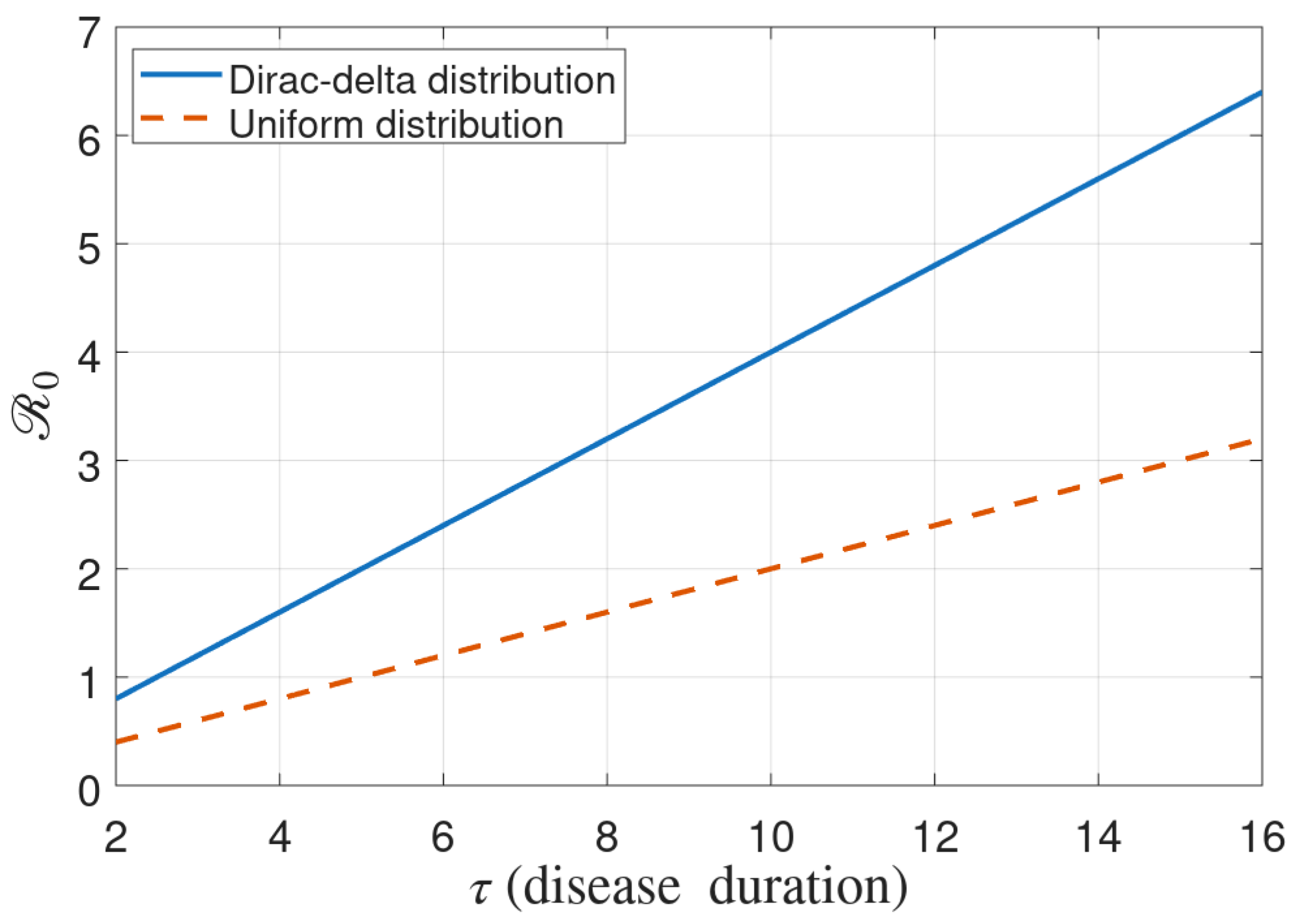
Note. If we assume a uniform distribution for recovery and death throughout the infectious period τ , the basic reproduction number is given by R 0 = β ^ ( 1 ϵ ρ ^ 0 ) τ 2 . This is because the uniform distribution spreads the likelihood of recovery or death evenly over time, effectively reducing the average infectious period considered in the calculation. In contrast, if we assume that infected individuals recover or die precisely after a fixed time τ , the basic reproduction number becomes R 0 = β ^ ( 1 ϵ ρ ^ 0 ) τ . Here, the entire infectious period contributes fully to disease transmission, leading to a higher value of R 0 . This highlights the critical importance of incorporating time-distributed recovery and death rates into the model to estimate R 0 more accurately.
A plot of R 0 for both the Dirac delta distributions and the uniform distributions of the recovery and death rates is shown in Figure 2.

3.2. Final Size of Epidemic

Let S ^ f be the final size of the susceptible compartment for asymptotically large time, lim t S ^ ( t ) = S ^ f . Integrating Equation (11) from 0 to with respect to t, we get
S ^ f S ^ 0 = 0 J ^ ( ζ ) d ζ .
On the other hand, integrating equation
d S ^ ( t ) d t = β ^ N S ^ ( t ) ( 1 ϵ ρ ^ ( t ) ) I ^ ( t ) ,
we obtain
ln S ^ f S ^ 0 = β ^ N 0 ( 1 ϵ ρ ^ ( ζ ) ) I ^ ( ζ ) d ζ .
Furthermore,
I ^ ( t ) = 0 t J ^ ( ζ ) d ζ R ^ ( t ) D ^ ( t ) = 0 t J ^ ( ζ ) d ζ 0 t 0 ζ r ^ ( ζ ξ ) + d ^ ( ζ ξ ) J ^ ( ξ ) d ξ d ζ = 0 t J ^ ( ζ ) 0 ζ r ^ ( ζ ξ ) + d ^ ( ζ ξ ) J ^ ( ξ ) d ξ d ζ .
Multiplying this equation by ( 1 ϵ ρ ^ ( t ) ) and integrating from 0 to with respect to t, we obtain
0 ( 1 ϵ ρ ^ ( t ) ) I ^ ( t ) d t = 0 ( 1 ϵ ρ ^ ( t ) ) ( 0 t [ J ^ ( ζ ) 0 ζ ( r ^ ( ζ ξ ) + d ^ ( ζ ξ ) ) J ^ ( ξ ) d ξ ] d ζ ) d t .
We change the order of integration with respect to ζ and t to get
0 ( 1 ϵ ρ ^ ( t ) ) I ^ ( t ) d t = 0 ζ ( 1 ϵ ρ ^ ( t ) ) [ J ^ ( ζ ) 0 ζ r ^ ( ζ ξ ) + d ^ ( ζ ξ ) J ^ ( ξ ) d ξ ] d t d ζ .
Let V 1 ( ζ ) = ζ ( 1 ϵ ρ ^ ( t ) ) d t . Then we can write
0 ( 1 ϵ ρ ^ ( t ) ) I ^ ( t ) d t = 0 J ^ ( ζ ) V 1 ( ζ ) d ζ 0 0 ζ r ^ ( ζ ξ ) + d ^ ( ζ ξ ) J ^ ( ξ ) V 1 ( ζ ) d ξ d ζ = 0 J ^ ( ξ ) V 1 ( ξ ) d ξ 0 ξ r ^ ( ζ ξ ) + d ^ ( ζ ξ ) V 1 ( ζ ) d ζ J ^ ( ξ ) d ξ = 0 [ V 1 ( ξ ) ξ r ^ ( ζ ξ ) + d ^ ( ζ ξ ) V 1 ( ζ ) d ζ ] J ^ ( ξ ) d ξ .
Furthermore,
ξ ( r ^ ( ζ ξ ) + d ^ ( ζ ξ ) ) V 1 ( ζ ) d ζ = ξ ζ r ^ ( ζ ξ ) + d ^ ( ζ ξ ) ( 1 ϵ ρ ^ ( t ) ) d t d ζ = ξ ξ t r ^ ( ζ ξ ) + d ^ ( ζ ξ ) d ζ ( 1 ϵ ρ ^ ( t ) ) d t ,
with V 1 ( ξ ) = ξ ( 1 ϵ ρ ^ ( t ) ) d t gives
V 1 ( ξ ) ξ r ^ ( ζ ξ ) + d ^ ( ζ ξ ) V 1 ( ζ ) d ζ = ξ 1 ξ t r ^ ( ζ ξ ) + d ^ ( ζ ξ ) d ζ ( 1 ϵ ρ ^ ( t ) ) d t .
Inequality
1 ξ t r ^ ( ζ ξ ) + d ^ ( ζ ξ ) d ζ < 1
follows from Condition (10). For some particular choice of functions r ^ ( ζ ) and d ^ ( ζ ) , a more precise estimate can be obtained. We have
V 1 ( ξ ) ξ r ^ ( ζ ξ ) + d ^ ( ζ ξ ) V 1 ( ζ ) d ζ ξ ( 1 ϵ ρ ^ ( t ) ) d t .
Therefore,
0 ( 1 ϵ ρ ^ ( t ) ) I ^ ( t ) d t 0 ξ ( 1 ϵ ρ ^ ( t ) ) J ^ ( ξ ) d t d ξ .
From (15), we have
d ρ ^ ( t ) d t = P ( m ^ ( t ) ) ( 1 ρ ^ ( t ) ) P ( m ^ ( t ) ) ( 1 ϵ ρ ^ ( t ) ) .
Integrating this inequality from 0 to t, we get
( 1 ϵ ρ ^ ( t ) ) = ( 1 ϵ ρ ^ 0 ) e ϵ 0 t P ( m ^ ( I ^ ( ζ ) ) ) d ζ ,
where ρ ^ 0 = ρ ^ ( 0 ) 0 . For simplicity of calculation, we assume that P ( m ^ ( I ^ ( ζ ) ) ) k . This implies ( 1 ϵ ρ ^ ( t ) ) ( 1 ϵ ρ ^ 0 ) e ϵ k t and consequently
0 ( 1 ϵ ρ ^ ( t ) ) I ^ ( t ) d t 0 ξ ( 1 ϵ ρ ^ 0 ) e ϵ k t d t J ^ ( ξ ) d ξ ( 1 ϵ ρ ^ 0 ) ϵ k 0 J ^ ( ξ ) d ξ .
From this inequality and (20), (21), we get the following estimate for the final size of epidemic:
ln S ^ 0 S ^ f S ^ 0 S ^ f β ^ ( 1 ϵ ρ ^ 0 ) N ϵ k .
Set x = S ^ f / S ^ 0 , Λ = β ^ ( 1 ϵ ρ ^ 0 ) S ^ 0 / N ϵ k . Then Inequality (22) can be written as follows:
ln x x 1 Λ .
Denote G ( x ) = ln x x 1 . That means G ( x ) Λ . Clearly, G ( x ) is a strictly decreasing function in ( 0 , 1 ) , lim x 0 + G ( x ) = and lim x 1 G ( x ) = 1 . Suppose that Λ > 1 . Then there exists a unique value x * ( 0 , 1 ) such that G ( x * ) = Λ . If  G ( a ) Λ for some x, then x x * . Note that
x * 1 Λ = N ϵ k β ^ ( 1 ϵ ρ ^ 0 ) S ^ 0 .
Hence, the lower bound of final size of epidemic x * is proportional to both k, the minimal probability of vaccination and ϵ , the vaccine effectiveness.

4. Numerical Simulations

4.1. Simulation of the Age-Independent Model

4.1.1. Effect of Memory Kernel

In this section, we illustrate the effect of information-based vaccination decisions on the epidemic progression with the numerical simulations of the reduced model without age distribution (11)–(15). We consider the distributed rate functions r ^ ( t ) and d ^ ( t ) as used in [26], r ^ ( t ) = p 0 f 1 ( t ) and d ^ ( t ) = ( 1 p 0 ) f 2 ( t ) where
f 1 ( t ) = 1 b 1 a 1 Γ ( a 1 ) t a 1 1 e t b 1 and f 2 ( t ) = 1 b 2 a 2 Γ ( a 2 ) t a 2 1 e t b 2 ,
with the values of parameters a 1 = 8.06275 , b 1 = 2.21407 , a 2 = 6.00014 , b 2 = 2.19887 and p 0 = 0.97 .
Let us consider the information index in the form [60]
m ^ ( t ) = 0 t K t i m e ( ζ ) I ^ ( t ζ ) d ζ ,
where the kernel K t i m e corresponds to the information about the spread of infection. We consider two types of kernels, with memory decay:
K t i m e ( ζ ) = a e a ζ ,
where a > 0 is the decay rate, and with memory acquisition-decay:
K t i m e ( ζ ) = b d d b ( e b ζ e d ζ ) ,
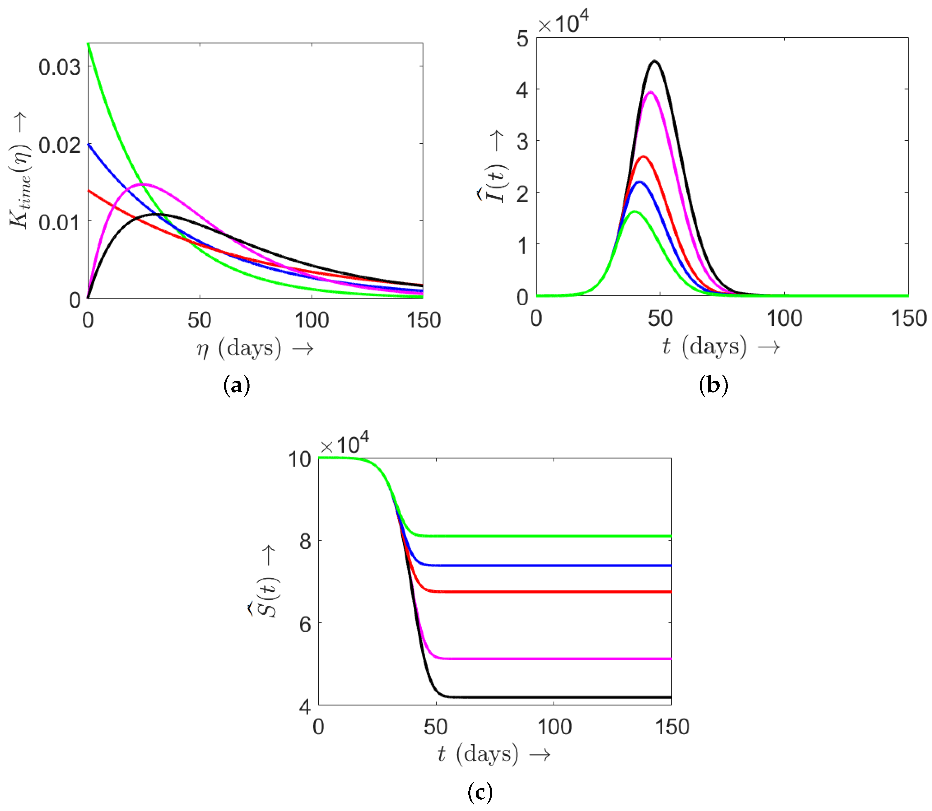
where 0 < b < d (Figure 3a). The exponentially fading kernel describes that the information for vaccination decision declines with time. The acquisition-decay kernel describes the fact of acquisition of information followed by a fading of memory.
Let us note that both kernels are normalized in such a way that their integrals from 0 to infinity equal 1. Large values of a in the first kernel correspond to the short-term memory, while small a to the long-term memory. Similarly, parameters of the second kernel determine the corresponding memory distribution. We see below how the memory distribution influences epidemic progression.
To complete the formulation of the model, we define function P ( m ^ ) as follows [62]:
P ( m ^ ) = k + m i n c m ^ m 0 H e v m ^ m 0 , 1 k .
Here, k is the minimal probability of vaccination independent of information, k ( 0 , 1 ) , c is a non-negative constant, H e v ( · ) is the Heaviside function. This function equals k for m ^ 0 , it has a linear growth on some interval of positive values of m ^ , and it equals 1 for m ^ sufficiently large.
Numerical simulations of Systems (11)–(15) are presented in Figure 3b,c for the values of parameters N = 10 5 , β ^ = 0.4 , S ^ ( 0 ) = N 1 , I ^ ( 0 ) = 1 , R ^ ( 0 ) = 0 , D ^ ( 0 ) = 0 , ρ ^ ( 0 ) = 0 , k = 0.02 , c = 10 4 , m 0 = 500 , ϵ = 1 and different values of parameters a , b , d that determine the memory kernels.
We note that the beginning of the epidemic outbreak does not depend on the parameters and on the kernel type. However, further epidemic progression is different. For larger values of a, the maximal number of infected individuals and their total number is less than for small values of a. Similarly, the final size of susceptible individuals is larger. Hence, the short-term memory is more efficient to restrain epidemic progression. A similar conclusion holds for the second kernel. Memory kernel influences epidemic progression during the outbreak. Since the duration of the outbreak is approximately 30 days, longer memory does not influence it.

4.1.2. Impact of Vaccine Effectiveness and Decaying Memory

The success of vaccination in preventing an epidemic depends on two key factors: vaccine effectiveness and vaccine hesitancy. To study the combined impact of these factors on epidemic progression, we utilize an exponentially decaying memory kernel defined as
K t i m e ( ζ ) = a e a ζ
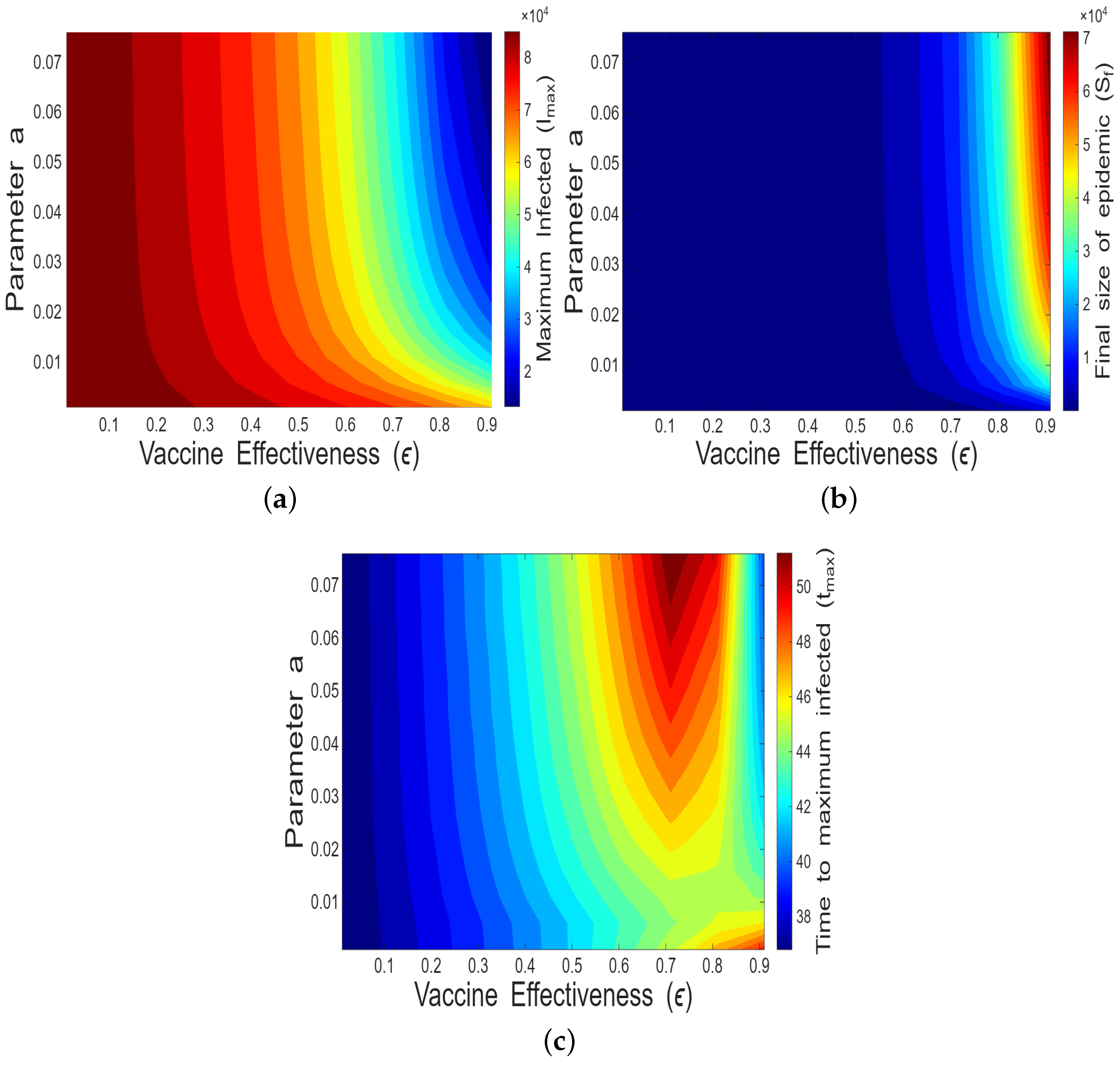
where a ranges from 0 to 0.08, and vaccine effectiveness ϵ varies between 0 and 1. All other parameter values are kept the same as before. The results are shown in Figure 4. From Figure 4a, it can be observed that even with high vaccine effectiveness ( ϵ between 0.8 and 1), a small value of a leads to a large epidemic outbreak. This is because smaller values of a correspond to a long-range memory effect, which causes vaccination decisions to be less responsive to current disease conditions, thus allowing for more significant outbreaks. In contrast, larger values of a indicate a short-range memory kernel, which appears to be more effective in controlling the epidemic as it allows for more adaptive and responsive vaccination strategies based on recent disease data. Similarly, when vaccine effectiveness is low, the epidemic peak remains high across all values of a. This underscores the fact that even a highly adaptive vaccination strategy (high a) cannot compensate for a vaccine with low effectiveness. Therefore, both a responsive vaccination approach (high a) and a highly effective vaccine (high ϵ ) are necessary to significantly reduce the epidemic size and avoid large outbreaks. Figure 4b,c show the respective plots for final size of epidemic ( S ^ f ) and the time to maximum infected ( t m ).

4.1.3. Impact of P ( m ^ )

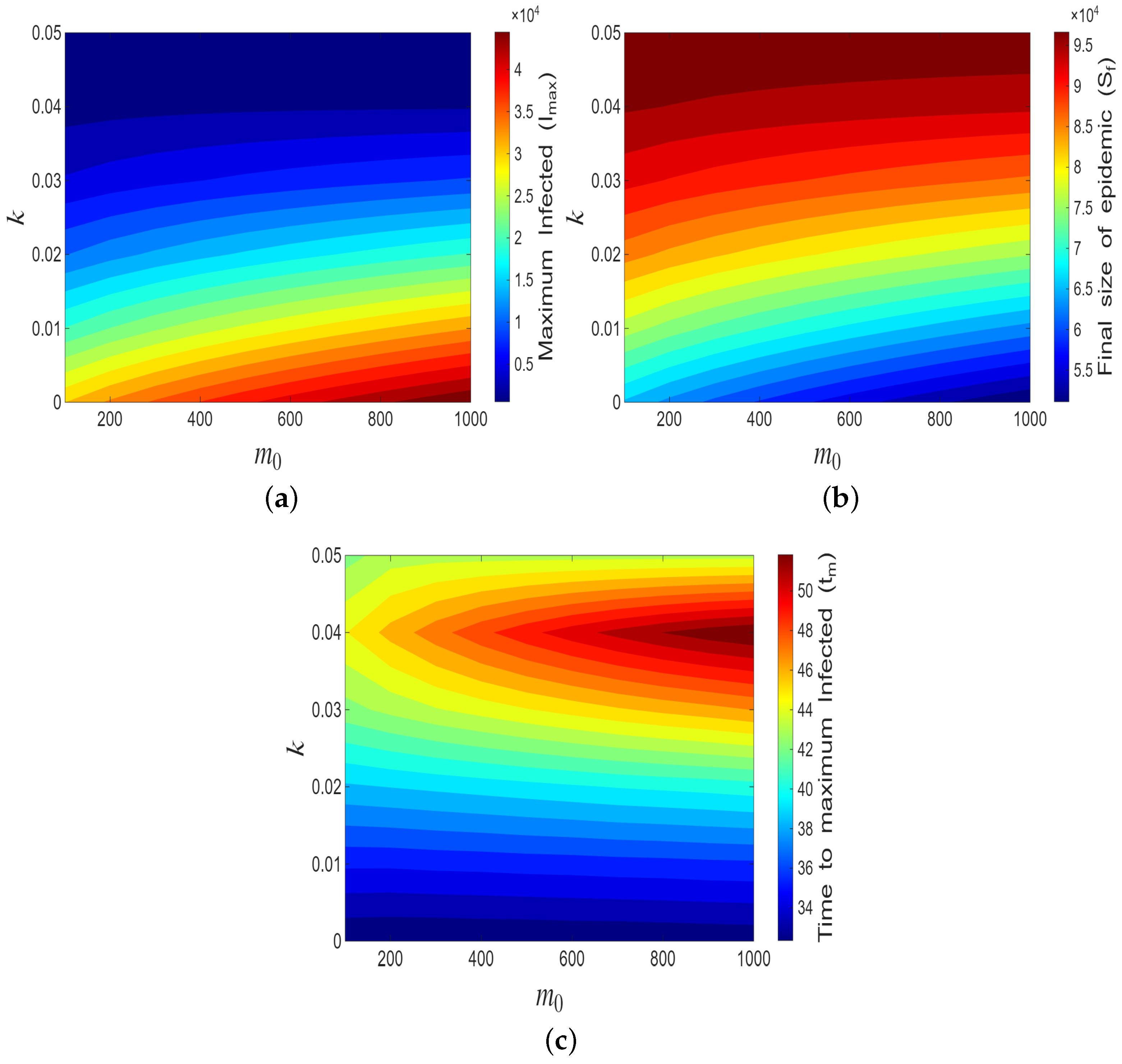
Finally, we explore how the probability of vaccine uptake, influenced by information, impacts epidemic dynamics. Specifically, we analyze the effect of varying two key parameters: k, the minimum probability of vaccine uptake, and  m 0 , the threshold of the information index beyond which people are more likely to vaccinate. The results are shown in Figure 5. Figure 5a illustrates that increasing m 0 results in a higher peak of infection for a given k. This suggests that if the population is slow to become informed or does not perceive the need for early vaccination, larger outbreaks can occur. In contrast, a higher k mitigates this risk, indicating that when a higher baseline willingness to vaccinate exists, the epidemic’s intensity is reduced. Figure 5b,c further demonstrate how these parameters influence the final epidemic size and the time to peak infection. These results underscore the importance of timely public awareness and a baseline readiness to vaccinate in controlling outbreaks and reducing their impact.

4.1.4. Sensitivity Analysis

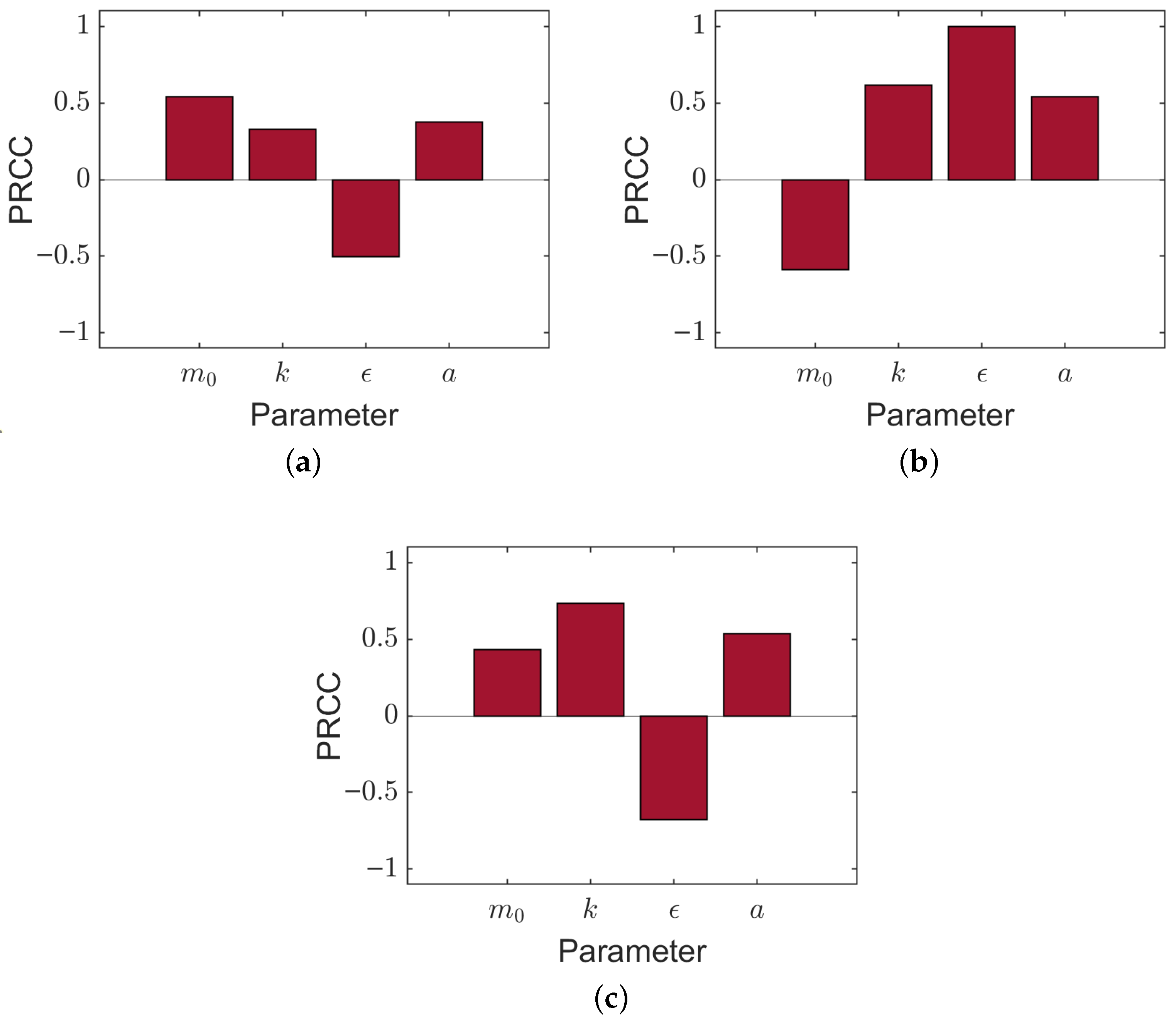
We assess the impact of the model parameters m 0 , k, ϵ and a on key features of the model outcomes, namely the maximum number of infected ( I ^ m ), the final epidemic size ( S ^ f ), and the time to maximum number of infected ( t m ). We compute Partial Rank Correlation Coefficients (PRCCs) [63] of the above-mentioned parameters. These coefficients were calculated by correlating the selected parameters with each of the model outcomes, providing a measure of the sensitivity of the model. For the PRCC calculation in MATLAB 2022b, the inbuilt corr function was employed. Specifically, residuals were obtained using linear regression via the regress function, and PRCC values were computed by correlating the residuals of the parameters with those of the outcomes.
In this analysis, 1000 samples were drawn from the feasible regions of the parameters using Latin Hypercube Sampling. The corresponding PRCC values are illustrated in the bar diagrams in Figure 6. The sensitivity analysis shows that ϵ and m 0 are the most significant parameters affecting I ^ m and S ^ f , while ϵ and k appear to be the most significant parameters affecting the time to maximum infected t m .

4.2. Simulation of the Age-Dependent Model

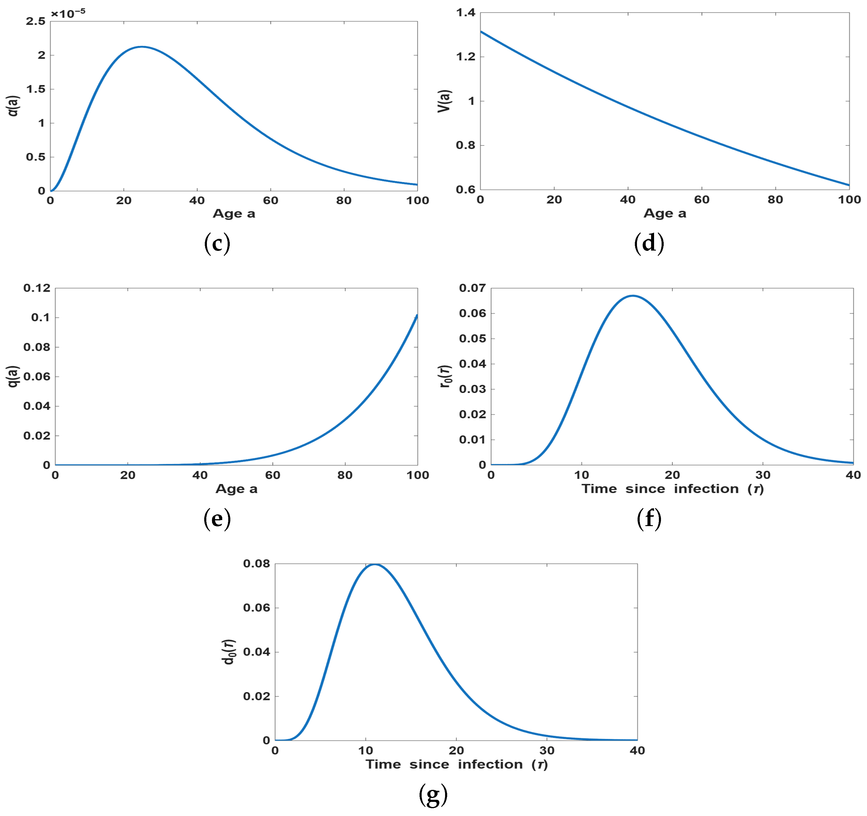
Now we perform the numerical simulation of the age-dependent Model (6)–(8). The model is simulated over the age domain a [ 0 , 100 ] and time domain t [ 0 , 100 ] . The associated age-dependent parameters and initial conditions are taken from [58]. The initial susceptible population is
S ( a , 0 ) = N ( 2.5666 × 10 11 a 5 5.428 × 10 9 a 4 + 3.67 × 10 7 a 3
1.086 × 10 5 a 2 + 0.0001539 a + 0.0125 ) ,
where N = 10 7 (see Figure 7a). The initial infected population is (see Figure 7b)
I ( a , 0 ) = 1 , a [ 20 , 30 ] , 0 , otherwise . .
Vaccination coverage is initialized as ρ ( a , 0 ) = 0 . The age-dependent transmission rate α ( a ) is defined using a gamma distribution:
α ( a ) = c α p ( a ) , α p ( a ) = a p 1 e a / q q p Γ ( p ) ,
with parameters p = 2.91955 , q = 12.9779 , and scaling constant c = 1 × 10 3 (see Figure 7c). V ( a ) is taken as the following exponential function (see Figure 7d)
V ( a ) = 10 a v b v a , a v = 5.92968 , b v = 0.003263 .
The time-distributed age-dependent recovery and death rates r ( a , t ) and d ( a , t ) are given, respectively, by
r ( a , t ) = ( 1 q ( a ) ) r 0 ( t ) , d ( a , t ) = q ( a ) d 0 ( t ) ,
where
r 0 ( t ) = t a 1 1 e t / b 1 b 1 a 1 Γ ( a 1 ) , d 0 ( t ) = t a 2 1 e t / b 2 b 2 a 2 Γ ( a 2 ) ,
with parameters a 1 = 8.06275 , b 1 = 2.21407 , a 2 = 6.00014 , and b 2 = 2.19887 ; q ( a ) is the age-dependent disease fatality profile as follows:
q ( a ) = 2.126 × 10 12 a 5.341 .
Plots of q ( a ) , r 0 ( t ) , and d 0 ( t ) are depicted in Figure 7e–g. Initially we chose the following memory kernel:
K time ( ζ ) = r e r ζ , r = 0.04 ;
however, later, we considered age dependency in memory kernel. Then, the age-structured information index is
m ( a , t ) = 0 t K time ( ζ ) I ( a , t ζ ) d ζ .
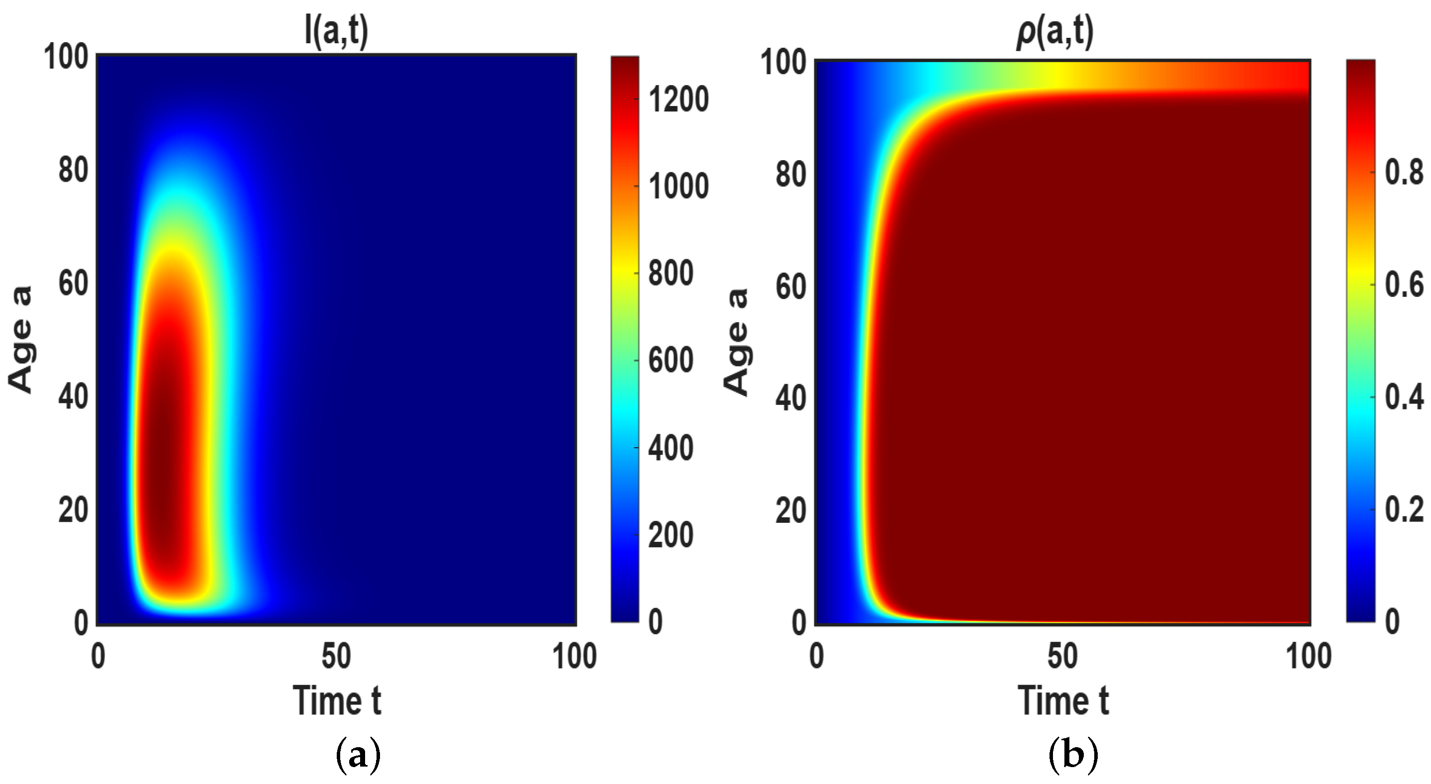
The choice of P ( m ( a , t ) ) is kept the same as in Equation (24). The simulation results for the age-dependent model (6)–(8) are shown in Figure 8. Although the initial infection is seeded in the age group 20–30, it rapidly propagates across a broader age range, approximately from 10 to 60 years, with the highest infection intensity observed among individuals aged 15–40. The evolution of ρ ( a , t ) indicates that as infection levels increase, the proportion of vaccinated individuals also rises, reaching near saturation across almost all age classes within a short time span. This behavior is driven by the choice r = 0.04 , which corresponds to a very strong short-term memory-based response (see Figure 3 for comparison). Vaccination coverage in older age groups exhibits a slight delay but eventually attains similarly high levels.

4.2.1. Impact of S 0 ( a )

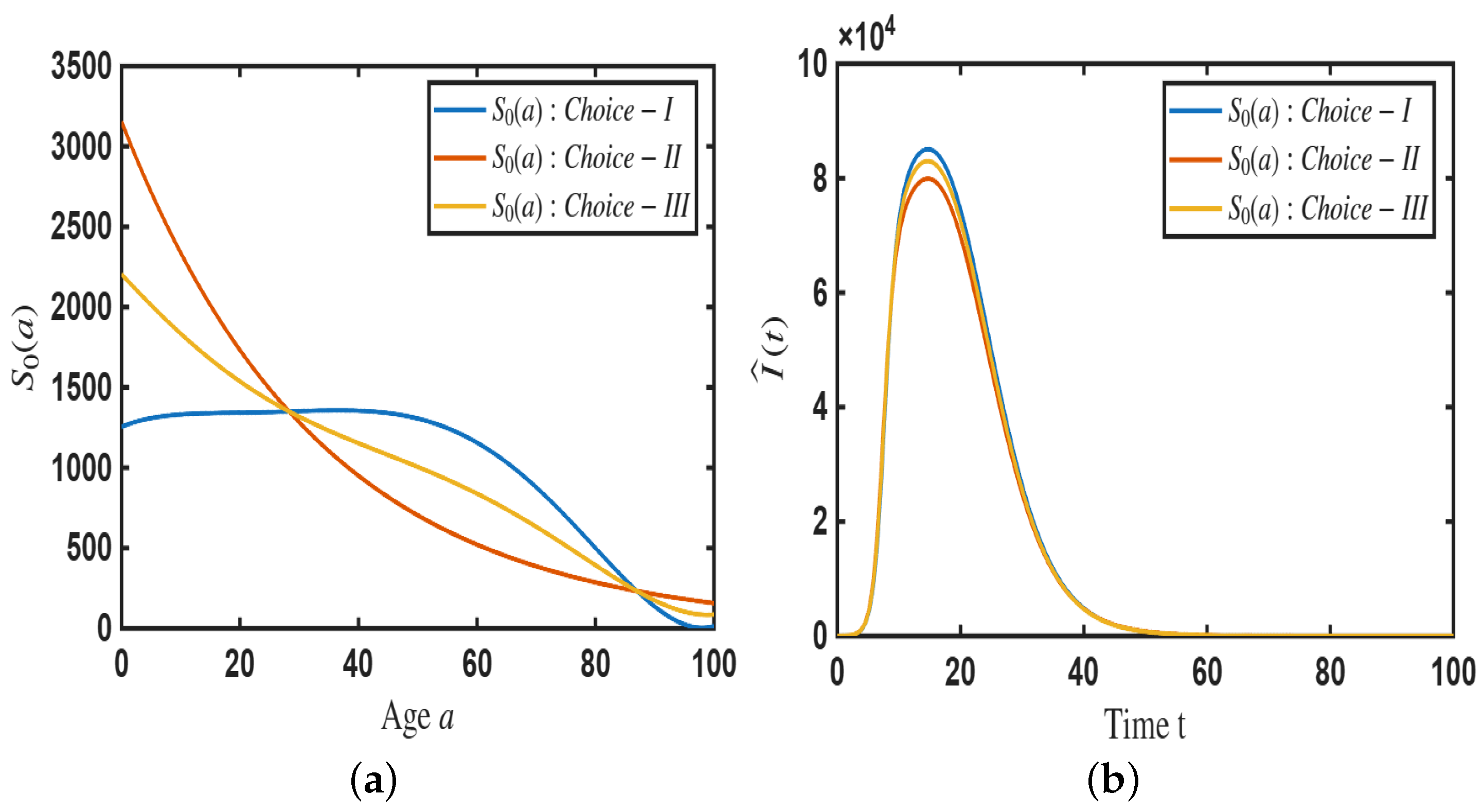
To investigate the impact of the initial age-dependent population structure on epidemic dynamics, we consider three choices of S 0 ( x ) , shown in Figure 9a. These choices differ in the relative distribution while maintaining the the same total population. Numerical simulations of Systems (6)–(8) are performed, and the epidemic evolution is quantified using the total number of infected individuals across all ages,
I ^ ( t ) = 0 100 I ( a , t ) d a ,
as illustrated in Figure 9b. The results indicate that the peak magnitude of I ^ ( t ) is sensitive to the initial age distribution of susceptible individuals although the total population is the same.

4.2.2. Impact of Age-Dependent Memory Kernel

Now we consider that the memory kernel depends on both time and age. If the age- and time-dependent memory kernel is denoted by K ( a , t ) , then the information index is given by
m ( a , t ) = 0 t K ( a , τ ) I ( a , t τ ) d τ .
We consider three alternative forms of the memory kernel K ( a , τ ) .
  • Choice-I:
K ( a , t ) = 0.04 e 0.04 t , t 0 .
This signifies a memory kernel that decays at the same rate across all ages.
  • Choice-II:
K ( a , t ) = 0.02 e 0.02 t , a < 50 , 0.06 e 0.06 t , a 50 , t 0 .
This choice accounts for stronger responsiveness of older individuals to epidemic information.
  • Choice-III:
K ( a , t ) = 0.02 + 0.03 e ( a 60 ) 2 / ( 2 σ 2 ) exp 0.02 + 0.03 e ( a 60 ) 2 / ( 2 σ 2 ) t , t 0 .
This yields a peak memory sensitivity around age 60, decreasing smoothly away from the peak.
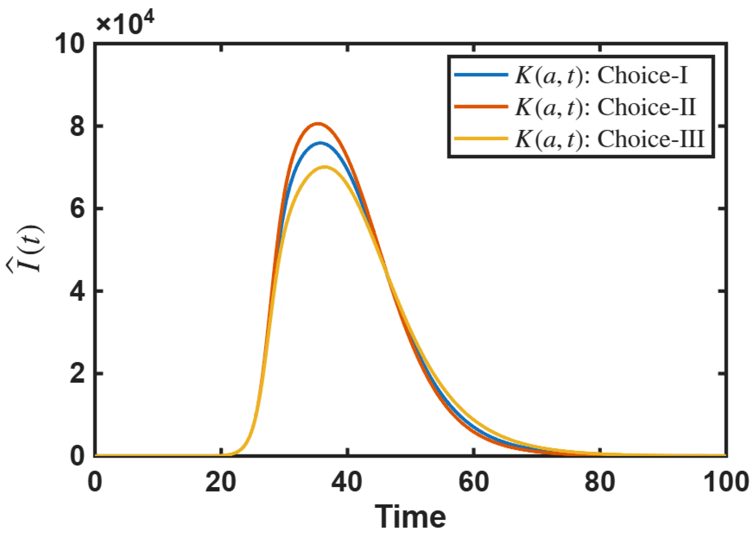
The plot of I ^ ( t ) for different choices of the age-dependent memory kernel K ( a , t ) is shown in Figure 10. Choice-III gives the lowest epidemic peak compared to the other choices. This result is consistent with the results shown in Figure 9. In Figure 9, the blue curve gives the highest epidemic peak, which corresponds to Choice-I of S 0 , where there is a significant and almost constant portion of the population in the age groups up to 70 years. Since Choice-III of K ( a , t ) concentrates memory sensitivity around age 60, decreasing smoothly away from the peak, it appears to be the most effective among the other two.

5. Discussion

This work focuses on the investigation of epidemic models incorporating time-distributed recovery and death rates, along with information-driven vaccination decisions. Similar to the previous models [11,26,61], the evolution of the number of susceptible individuals S ^ ( t ) and infected individuals I ^ ( t ) is determined through the number of newly infected individuals J ^ ( t ) = β ^ S ^ ( t ) I ^ ( t ) / N . This approach allows a more accurate understanding of the epidemic progression than the conventional SIR model. An age-distributed model with distributed recovery and death rate was introduced in [58], and the influence of vaccination waning was studied in [11].
In this work, our primary objective is to analyze epidemic progression over a relatively short duration, where demographic changes are minimal. Specifically, the rate of transition between age groups is negligible. For example, if we study the epidemic model with a time unit of ‘days’ over a range of a few months, the natural death rate is approximately 1 / ( 365 × 100 ) days 1 0.000027 days 1 , which is negligible. Additionally, vertical transmission is not considered. That is why we do not include demographic factors like natural birth and death in our model.
Vaccination campaign during the COVID-19 pandemic was accompanied by widespread hesitancy and resistance [64,65,66] related to the precipitation in the vaccine development and by the reporting of some adverse effects. This vaccination avoidance was reinforced by the rumors through various social networks and various informal mass media [67,68]. Though it is difficult to estimate exactly the influence of available information on the vaccination hesitancy, we can reasonably assume that the willingness to vaccinate is proportional to the number of infected individuals [69,70]. Moreover, information-based decisions include some memory effect which is taken into account in the model through the memory kernel.
In order to describe the effects of age-specific vaccination decisions on epidemic progression, we propose an integro-differential system of equations for susceptible, infected, recovered, dead individuals, and for the proportion of vaccinated individuals. To mathematically justify the proposed model, we proved the existence and uniqueness of a positive solution with the help of fixed point theory. Moreover, for the model without age distribution, we derived the analytical expression for R 0 and a bound for the final size of epidemic. When assuming a uniform distribution of recovery and death throughout the infectious period, R 0 is underestimated compared to the case where recovery or death occurs precisely after a fixed time. This discrepancy arises because a uniform distribution effectively shortens the average infectious period contributing to disease transmission, thereby reducing R 0 . In contrast, assuming a fixed recovery or death time captures the full infectious period, leading to a more accurate and typically higher estimate of R 0 . This highlights the critical importance of incorporating time-distributed recovery and death rate into the model, as it ensures a more accurate estimation of R 0 , which is essential for understanding the dynamics of disease transmission and designing effective control strategies.
The model developed in this work is able to capture the influence of age-specific information-based vaccination decisions. In the prediction regarding the epidemic growth, we need more detailed age-specific data to appropriately estimate the distributed parameters involved in the model. However, in a simpler case, for the model without age distribution, we show the effect of information on epidemic progression. The kernel K t i m e ( ζ ) involved in the information index m ^ ( t ) reflects the information about the effect of vaccination on past epidemic progression.
We observe that the initial pattern of the epidemic outbreak is similar for different kernels since the memory effect is not yet influential, and the epidemic progression is mainly determined by the initial conditions and the transmission behavior of the disease. However, as the epidemic progresses and more information about the disease becomes available, the information-based vaccination decisions can have a significant impact on the course of the epidemic. Short-term memory appears to be more efficient to restrain the epidemic burst because it allows for more responsive and adaptive vaccination decisions based on the most recent information about the disease. The question of age-distributed vaccination decisions require further investigations and availability of relevant data. In the case of COVID-19 epidemic, young age groups provide, at the same time, a higher rate of epidemic transmission and stronger vaccination resistance due to lower mortality rate.
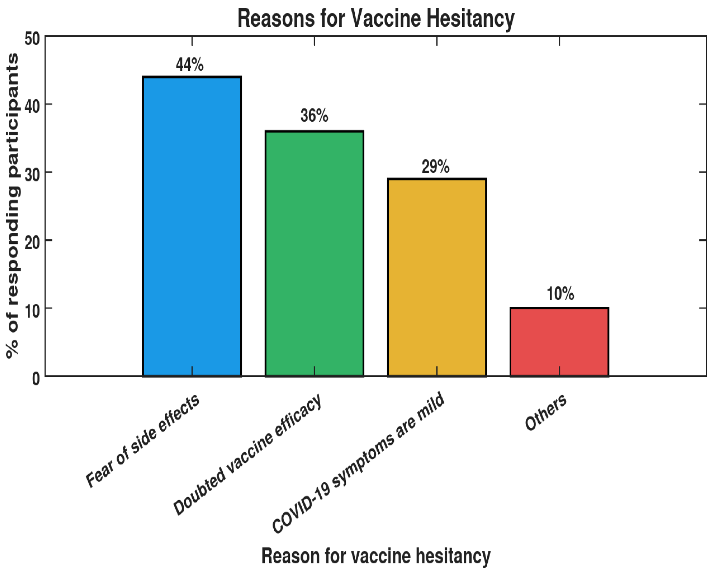
The success of vaccination in preventing an epidemic depends on two key factors: vaccine effectiveness and vaccine hesitancy, provided that the vaccine supply is sufficient to meet the requirements. We studied the combined impact of these factors on epidemic progression. Our simulation results show that both a responsive vaccination approach (high a) and a highly effective vaccine (high ϵ ) are necessary to significantly reduce epidemic size and avoid large outbreaks. Throughout this work, we assumed that the vaccine decisions and vaccine effectiveness are independent of each other. However, existing literature shows that vaccine hesitancy is significantly influenced by information regarding vaccine effectiveness. In the context of COVID-19, study [71] indicates that 36 % of participants expressed vaccine hesitancy because they were unsure about vaccine effectiveness (see Figure 11). Similar observations have been made in [72,73]. These results suggest that vaccine decision-making is implicitly dependent on vaccine effectiveness, which needs to be explored in future research.
Furthermore, in this study, the simulation results emphasize the critical role of public awareness and baseline willingness to vaccinate in controlling the severity of outbreaks. A higher threshold for the information index, m 0 , leads to a delayed response in vaccination uptake, potentially resulting in larger epidemic peaks. Conversely, when the baseline probability of vaccination (k) is higher, even without strong information-based triggers, the epidemic’s impact is significantly mitigated. These findings underscore the importance of early and proactive public health communication strategies to ensure timely vaccination and reduce outbreak intensity. The impacts of the age-dependent initial susceptible population and the age-dependent memory kernel are studied. The results show that the epidemic size depends on the memory kernel K ( a , t ) and initial susceptible population S 0 ( a ) . Moreover, these impacts are interrelated. The distribution of S 0 ( a ) influences the effectiveness of the age-dependent memory kernel.

6. Conclusions

The model presented in this work offers a novel framework for studying the influence of human behavior-dependent vaccination decisions on epidemic progression. The following conclusions can be drawn from this study:
  • The age-distributed model describes disease incidence J ( a , t ) , and incorporating age-dependent vaccination decisions with the help of a memory kernel enables us to describe how past epidemic information shapes the epidemic outbreak size.
  • The initial epidemic pattern is unaffected by the memory kernel, as memory effects are negligible at early stages. However, in later phases, the memory kernel significantly shapes epidemic progression, with short-term memory proving more effective in restraining outbreaks by enabling more adaptive vaccination responses to recent infection trends.
  • Along with high vaccine effectiveness ( ϵ ), responsive vaccination (i.e., a higher value of a) is also necessary to successfully reduce the outbreak size.
  • The impact of the baseline probability of vaccination (k) on outbreak control is studied.
  • Age-dependent initial susceptible population and age-dependent memory kernel can influence the size of epidemic outbreak.

Limitations and Future Directions

The model proposed in this work is based on some simplified assumptions. The model represents all infected individuals within a single compartment. However, many respiratory diseases, including COVID-19, exhibit distinct asymptomatic, pre-symptomatic, and symptomatic stages, each with different levels of infectiousness. These distinctions can substantially influence transmission dynamics and may alter the predicted effect of memory-based vaccination decisions. In addition, the model assumes that vaccine supply is always adequate to match behavioral demand. However, vaccination campaigns often face supply shortages, distribution delays, prioritisation strategies, and age-specific access constraints. These logistical factors can interact with information-driven vaccination behavior and age structure in nontrivial ways.
Although the present study considers an incidence-dependent information index m ( t ) , we acknowledge that real-world vaccination behavior is shaped by several additional factors, including hospitalization trends, perceived risk, and socio-behavioral influences. Incorporating these elements would require extending the model to include additional compartments or feedback mechanisms.
The present work can be extended by introducing stochasticity, entropy-based uncertainty quantification, and multi-parameter sensitivity analysis [74,75]. Such approaches will allow explicit assessment of how uncertainties in memory-kernel shape, behavioral responsiveness, vaccine effectiveness, and recovery/death distributions affect epidemic predictions.
Moreover, the current model can be further improved by introducing heterogeneous age-specific contact patterns, waning immunity, and more realistic vaccination scheduling [11,76,77]. Detailed methods can be adopted to calibrate age-dependent vaccination behavior using empirical data [76].
Incorporating these ideas in future extensions would allow the model to capture more realistic mixing patterns, improve parameter calibration, integrate immunity decay, and better quantify the robustness of predictions.

Author Contributions

Conceptualization, V.V.; Methodology, S.G.; Formal analysis, S.G.; Investigation, S.G.; Resources, M.B.; Writing—original draft, S.G.; Writing—review and editing, M.B. and V.V.; Visualization, V.V.; Supervision, M.B. and V.V. All authors have read and agreed to the published version of the manuscript.

Funding

Vitaly Volpert has been supported by the RUDN University Strategic Academic Leadership Program.

Data Availability Statement

The original contributions presented in this study are included in the article. Further inquiries can be directed to the corresponding author.

Conflicts of Interest

The authors declare no conflicts of interest.

Appendix A. Existence and Uniqueness of Positive Solution

In this section, we investigate the existence, uniqueness, and positivity of solution for Systems (5)–(8) with initial Conditions (9). We begin with some preliminary mathematical results.

Appendix A.1. Preliminary Results

We recall some definitions and results used to prove the existence and uniqueness results.
Definition A1.
Let f : S 1 S 2 be a single-valued mapping, where S 1 and S 2 are two non-empty sets. If for some x S 1 , f ( x ) = x , then x is called a fixed point of f.
Definition A2 ([78]).
Let ( M , d ) be a metric space and f : ( M , d ) ( M , d ) be a mapping. It is called a Banach contraction mapping if there exists a real number r [ 0 , 1 ) such that
d ( f ( x ) , f ( y ) ) r d ( x , y ) ,
for all x , y M .
Theorem A1 ([78]).
Let ( M , d ) be a complete metric space and f : ( M , d ) ( M , d ) be a Banach contraction mapping. Then f has a unique fixed point in x.
Before the existence and uniqueness theorem, we prove the positiveness of solution for Systems (5)–(8) in the following subsection.

Appendix A.2. Positiveness

Lemma A1.
If Condition (10) holds, then solutions S ( a , t ) , I ( a , t ) , R ( a , t ) , and D ( a , t ) of Models (5)–(9) are bounded by 0 and S 0 ( a ) + I 0 ( a ) .
Proof. 
First of all, from (8), we note that, for some a = a 1 and t = t 1 , ρ ( a 1 , t 1 ) = 1 implies ρ t ( a 1 , t 1 ) = 0 . Hence, if ρ ( a , 0 ) 0 , then 0 ρ ( a , t ) 1 , for all a , t . Initially, we have S ( a , 0 ) 0 for all a.
Now integrating Equation (6) with respect to t from 0 to t, we obtain
S ( a , t ) = S ( a , 0 ) e 0 t α ( a ) ( 1 ϵ ρ ( a , t ) ) 0 A M V ( y ) I ( y , t ) d y d t .
This proves the positivity of S ( a , t ) . Also, from (5), it is clear that R ( a , t ) and D ( a , t ) are positive for all a, t.
Moreover, we have
I ( a , t 0 ) = 0 t 0 J ( a , ζ ) d ζ R ( a , t 0 ) D ( a , t 0 ) ,
for some t = t 0 > 0 . With the initial conditions R ( a , 0 ) = D ( a , 0 ) = 0 , we integrate (5) from 0 to t 0 with respect to t:
R ( a , t 0 ) + D ( a , t 0 ) = 0 t 0 0 t r ( a , t ζ ) + d ( a , t ζ ) J ( a , ζ ) d ζ d t .
Changing the order of integration and using Assumption (10), we get the following:
R ( a , t 0 ) + D ( a , t 0 ) = 0 t 0 ζ t 0 r ( a , t ζ ) + d ( a , t ζ ) d t J ( a , ζ ) d ζ 0 t 0 J ( a , ζ ) d ζ .
Now, using Condition (A1), we obtain I ( a , t 0 ) 0 . Moreover,
S ( a , t ) + I ( a , t ) + R ( a , t ) + D ( a , t ) = S 0 ( a ) + I 0 ( a ) .
Thus, any solution of Systems (5)–(8) lies between 0 and S 0 ( a ) + I 0 ( a ) . □

Appendix A.3. Existence of Unique Positive Solution

We prove the existence of unique positive solution of Systems (5)–(8) for ( a , t ) [ 0 , A M ] × [ 0 , T ] , where A M , T ( 0 , ) .
Theorem A2.
If P ( m ) is a Lipschitz continuous function of m, then there exists a unique solution of Systems (5)–(8) in the domain M 5 , where
M = { Φ C [ 0 , A M ] × [ 0 , T ] , R : 0 Φ ( a , t ) S 0 ( a ) + I 0 ( a ) ,
( a , t ) [ 0 , A M ] × [ 0 , T ] } .
To prove this theorem, we use the complete metric space setting M , d and the metric d defined by
d ( Φ 1 , Φ 2 ) = sup ( a , t ) [ 0 , A M ] × [ 0 , T ] e δ t | Φ 1 ( a , t ) Φ 2 ( a , t ) | ,
where δ > 0 is a constant. The proof of completeness is as follows:
Lemma A2.
Consider the metric space M , d with
d ( Φ 1 , Φ 2 ) = sup ( a , t ) [ 0 , A M ] × [ 0 , T ] e δ t | Φ 1 ( a , t ) Φ 2 ( a , t ) | ,
where δ > 0 is a constant. Then M , d is complete.
Proof. 
Clearly, M is a closed subset of C [ 0 , A M ] × [ 0 , T ] , R . We know that C [ 0 , A M ] × [ 0 , T ] , R is complete with respect to the metric
d sup ( Φ 1 , Φ 2 ) = sup ( a , t ) [ 0 , A M ] × [ 0 , T ] | Φ 1 ( a , t ) Φ 2 ( a , t ) | .
Hence, ( M , d sup ) is also complete.
  • Now, we have
e δ T d sup ( Φ 1 , Φ 2 ) d ( Φ 1 , Φ 2 ) d sup ( Φ 1 , Φ 2 ) ,
which shows that d sup and d are equivalent metrics, and consequently, ( M , d ) is a complete metric space. □
For any given function Φ M , we set
m Φ ( a , t ) = m ( Φ ( a , t ) ) .
Then for this choice of m Φ ( a , t ) and P ( m Φ ( a , t ) ) , equation
ρ ( a , t ) t = P ( m Φ ( a , t ) ) ( 1 ρ ( a , t ) ) ,
with ρ ( a , 0 ) = ρ 0 ( a ) has a unique solution ρ Φ ( a , t ) satisfying equation
( 1 ρ Φ ( a , t ) ) = ( 1 ρ 0 ( a ) ) e 0 t P ( m Φ ( a , ζ ) ) d ζ .
For this given choice of Φ ( a , t ) and ρ Φ ( a , t ) , equation
S ( a , t ) t = α ( a ) S ( a , t ) ( 1 ϵ ρ Φ ( a , t ) ) 0 A M V ( y ) Φ ( y , t ) d y ,
with S ( a , 0 ) = S 0 ( a ) has a unique solution (since the right-hand side is a Lipschitz continuous function in S) and the solution can be written as follows:
S Φ ( a , t ) = S 0 ( a ) e α ( a ) 0 t ( 1 ϵ ρ Φ ( a , ζ ) ) 0 A M V ( y ) Φ ( y , ζ ) d y d ζ .
Let
J Φ ( a , t ) = α ( a ) ( 1 ϵ ρ Φ ( a , t ) ) S Φ ( a , t ) 0 A M V ( y ) Φ ( y , t ) d y .
Then equation
I ( a , t ) t = α ( a ) ( 1 ϵ ρ Φ ( a , t ) ) S Φ ( a , t ) 0 A M V ( y ) Φ ( y , t ) d y 0 t r ( a , t ζ ) + d ( a , t ζ ) J Φ ( a , ζ ) d ζ ,
with I ( a , 0 ) = I 0 ( a ) has unique solution which can be written in the form
I Φ ( a , t ) = I 0 ( a ) + 0 t A ( a , ζ , Φ ) d ζ ,
where
A ( a , ζ , Φ ) = α ( a ) ( 1 ϵ ρ Φ ( a , ζ ) ) S 0 ( a ) e α ( a ) 0 ζ ( 1 ϵ ρ Φ ( a , ξ ) ) 0 A M V ( y ) Φ ( y , ξ ) d y d ξ 0 A M V ( y ) Φ ( y , ζ ) d y 0 ζ [ r ( a , ζ ξ ) + d ( a , ζ ξ ) α ( a ) ( 1 ϵ ρ Φ ( a , ξ ) ) S 0 ( a ) e α ( a ) 0 ξ ( 1 ϵ ρ Φ ( a , ν ) ) 0 A M V ( y ) Φ ( y , ν ) d y d ν 0 A M V ( y ) Φ ( y , ξ ) d y ] d ξ .
For further proof, we need the following lemma:
Lemma A3.
The map F : ( M , d ) ( M , d ) defined by equality
F ( Φ ) ( a , t ) = I 0 ( a ) + 0 t A ( a , ζ , Φ ) d ζ ,
where A ( a , ζ , Φ ) given in (A9) is well defined.
Proof. 
From (A6), we observe that
S Φ ( a , t ) t = ( α ( a ) ( 1 ϵ ρ Φ ( a , t ) ) S 0 ( a ) e α ( a ) 0 t ( 1 ϵ ρ Φ ( a , ξ ) ) 0 A M V ( y ) Φ ( y , ξ ) d y d ξ ) 0 A M V ( y ) Φ ( y , t ) d y .
Using this relation in (A9), we can write
A ( a , ζ , Φ ) = S Φ ( a , ζ ) ζ 0 ζ r ( a , ζ ξ ) + d ( a , ζ ξ ) S Φ ( a , ξ ) ξ d ξ ,
and
0 t A ( a , ζ , Φ ) d ζ = [ 0 t S Φ ( a , ζ ) ζ d ζ 0 t 0 ζ r ( a , ζ ξ ) + d ( a , ζ ξ ) S Φ ( a , ξ ) ξ d ξ d ζ ] .
We change the order of integration to get the following:
0 t A ( a , ζ , Φ ) d ζ = [ 0 t S Φ ( a , ζ ) ζ d ζ 0 t ξ t r ( a , ζ ξ ) + d ( a , ζ ξ ) d ζ S Φ ( a , ξ ) ξ d ξ ] = 0 t 1 ξ t r ( a , ζ ξ ) + d ( a , ζ ξ ) d ζ S Φ ( a , ξ ) ξ d ξ .
Note that S Φ ( a , ξ ) ξ 0 , and using Condition (10), we can write
0 t A ( a , ζ , Φ ) d ζ 0 t S Φ ( a , ξ ) ξ d ξ = S 0 ( a ) S Φ ( a , t ) S 0 ( a ) .
This implies the estimate
F ( Φ ) ( a , t ) = I 0 ( a ) + 0 t A ( a , ζ , Φ ) d ζ I 0 ( a ) + S 0 ( a ) .
If Φ 1 , Φ 2 M and Φ 1 = Φ 2 , then S Φ 1 = S Φ 2 and consequently A ( a , ζ , Φ 1 ) = A ( a , ζ , Φ 2 ) , and consequently F is well defined. □
In the following lemma, we show that F : ( M , d ) ( M , d ) is a contraction.
Lemma A4.
The map F : ( M , d ) ( M , d ) defined in Lemma A3 is a contraction.
Proof. 
From (A9), we have
A ( a , ζ , Φ ) = α ( a ) ( 1 ϵ ρ Φ ( a , ζ ) ) S 0 ( a ) e α ( a ) 0 ζ ( 1 ϵ ρ Φ ( a , ξ ) ) 0 A M V ( y ) Φ ( y , ξ ) d y d ξ 0 A M V ( y ) Φ ( y , ζ ) d y 0 ζ [ r ( a , ζ ξ ) + d ( a , ζ ξ ) α ( a ) ( 1 ϵ ρ Φ ( a , ξ ) ) S 0 ( a ) e α ( a ) 0 ξ ( 1 ϵ ρ Φ ( a , ν ) ) 0 A M V ( y ) Φ ( y , ν ) d y d ν 0 A M V ( y ) Φ ( y , ξ ) d y ] d ξ .
Let
Φ ^ ( a , ξ ) = ( 1 ϵ ρ Φ ( a , ξ ) ) 0 A M V ( y ) Φ ( y , ξ ) d y .
Then the above expression for A ( a , ζ , Φ ) can be written as follows:
A ( a , ζ , Φ ) = α ( a ) S 0 ( a ) e α ( a ) 0 ζ Φ ^ ( a , ξ ) d ξ Φ ^ ( a , ζ ) 0 ζ [ r ( a , ζ ξ ) + d ( a , ζ ξ ) α ( a ) S 0 ( a ) e α ( a ) 0 ξ Φ ^ ( a , ν ) d ν Φ ^ ( a , ξ ) ] d ξ .
For any Φ 1 ( a , t ) , Φ 2 ( a , t ) M ,
| F ( Φ 1 ) ( a , t ) F ( Φ 2 ) ( a , t ) | 0 t | A ( a , ζ , Φ 1 ) A ( a , ζ , Φ 2 ) | d ζ .
Next,
| A ( a , ζ , Φ 1 ) A ( a , ζ , Φ 2 ) | = α ( a ) S 0 ( a ) | [ e α ( a ) 0 ζ Φ ^ 1 ( a , ξ ) d ξ Φ ^ 1 ( a , ζ ) 0 ζ ( r ( a , ζ ξ ) + d ( a , ζ ξ ) ) e α ( a ) 0 ξ Φ ^ 1 ( a , ν ) d ν Φ ^ 1 ( a , ξ ) d ξ ] [ e α ( a ) 0 ζ Φ ^ 2 ( a , ξ ) d ξ Φ ^ 2 ( a , ζ ) 0 ζ ( r ( a , ζ ξ ) + d ( a , ζ ξ ) ) e α ( a ) 0 ξ Φ ^ 2 ( a , ν ) d ν Φ ^ 2 ( a , ξ ) d ξ ] | ,
where
Φ ^ j ( a , ξ ) = ( 1 ϵ ρ Φ j ( a , ξ ) ) 0 A M V ( y ) Φ j ( y , ξ ) d y , j = 1 , 2 .
From Equation (A4), we observe that if ρ 0 ( a ) 0 , then ( 1 ϵ ρ Φ j ( a , ξ ) ) always non-negative, and hence Φ ^ j ( a , ξ ) is always non-negative, for j = 1 , 2 . To simplify forthcoming mathematical expressions, we use the notation
Δ ( a , . ) = Φ ^ 1 ( a , . ) Φ ^ 2 ( a , . ) ,
where ‘.’ stands for ξ , ζ and ν as per necessity.
| A ( a , ζ , Φ 1 ) A ( a , ζ , Φ 2 ) | = α ( a ) S 0 ( a ) | e α ( a ) 0 ζ Φ ^ 1 ( a , ξ ) d ξ Δ ( a , ζ ) 0 ζ ( r ( a , ζ ξ ) + d ( a , ζ ξ ) ) e α ( a ) 0 ξ Φ ^ 1 ( a , ν ) d ν Δ ( a , ξ ) d ξ + e α ( a ) 0 ζ Φ ^ 1 ( a , ξ ) d ξ e α ( a ) 0 ζ Φ ^ 2 ( a , ξ ) d ξ Φ ^ 2 ( a , ζ ) + 0 ζ ( r ( a , ζ ξ ) + d ( a , ζ ξ ) ) e α ( a ) 0 ξ Φ ^ 2 ( a , ν ) d ν e α ( a ) 0 ξ Φ ^ 1 ( a , ν ) d ν Φ ^ 2 ( a , ξ ) d ξ | .
For any p , q 0 , we have
| e p e q | | p q | , | e p | 1 .
Using the above inequalities, we get
| A ( a , ζ , Φ 1 ) A ( a , ζ , Φ 2 ) | α ( a ) S 0 ( a ) ( | Δ ( a , ζ ) | + 0 ζ ( r ( a , ζ ξ ) + d ( a , ζ ξ ) ) | Δ ( a , ξ ) | d ξ + α ( a ) Φ ^ 2 ( a , ζ ) 0 ζ | Δ ( a , ξ ) | d ξ + 0 ζ ( r ( a , ζ ξ ) + d ( a , ζ ξ ) ) α ( a ) 0 ξ | Δ ( a , ν ) | d ν Φ ^ 2 ( a , ξ ) d ξ ) .
Since Φ j ( a , ξ ) S 0 ( a ) + I 0 ( a ) and 0 ( 1 ϵ ρ Φ j ( a , ξ ) ) 1 , we can write
0 Φ ^ j ( a , ξ ) M , j = 1 , 2 ,
where
M = ( S 0 ( a ) + I 0 ( a ) ) 0 A M V ( y ) d y .
Hence,
| Δ ( a , ζ ) | = | ( 1 ϵ ρ Φ 1 ( a , ζ ) ) 0 A M V ( y ) Φ 1 ( y , ζ ) d y ( 1 ϵ ρ Φ 2 ( a , ζ ) ) 0 A M V ( y ) Φ 2 ( y , ζ ) d y | = | ( 1 ϵ ρ Φ 1 ( a , ζ ) ) 0 A M V ( y ) ( Φ 1 ( y , ζ ) Φ 2 ( y , ζ ) ) d y + 0 A M ϵ V ( y ) Φ 2 ( y , ζ ) d y ( ρ Φ 2 ( a , ζ ) ρ Φ 1 ( a , ζ ) ) | .
Let M 1 = 0 A M V ( y ) d y . Using the estimate 0 ( 1 ϵ ρ Φ 1 ( a , ξ ) ) 1 , we get, from the above equation,
| Δ ( a , ζ ) | M 1 e δ ζ d ( Φ 1 , Φ 2 ) + M | ρ Φ 1 ( a , ζ ) ρ Φ 2 ( a , ζ ) | .
From Relation (A4), we obtain the following inequalities:
| ρ Φ 1 ( a , ζ ) ρ Φ 2 ( a , ζ ) | | e 0 ζ P ( m Φ 1 ( a , ξ ) ) d ξ e 0 ζ P ( m Φ 2 ( a , ξ ) ) d ξ | | 0 ζ P ( m Φ 1 ( a , ξ ) ) d ξ 0 ζ P ( m Φ 2 ( a , ξ ) ) d ξ | 0 ζ | P ( m Φ 1 ( a , ξ ) ) P ( m Φ 2 ( a , ξ ) ) | d ξ .
We assume that function P m ( Φ ) = P ( m ( Φ ) ) is a Lipschitz continuous function of Φ , that is,
d ( P m ) ( Φ 1 ) , ( P m ) ( Φ 2 ) K d ( Φ 1 , Φ 2 ) ,
where K 0 is a constant. This implies the estimate
| P ( m Φ 1 ( a , ξ ) ) P ( m Φ 2 ( a , ξ ) ) | = | ( P m ) ( Φ 1 ( a , ξ ) ) ( P m ) ( Φ 2 ( a , ξ ) ) |
K e δ ξ d ( Φ 1 , Φ 2 ) .
Using (A11), we obtain
| ρ Φ 1 ( a , ζ ) ρ Φ 2 ( a , ζ ) | K d ( Φ 1 , Φ 2 ) 0 ζ e δ ξ d ξ = K d ( Φ 1 , Φ 2 ) e δ ζ δ ,
and consequently, we get
| Φ ^ 1 ( a , ζ ) Φ ^ 2 ( a , ζ ) | M 3 e δ ζ d ( Φ 1 , Φ 2 ) ,
where M 3 = M 1 + M K δ . From these relations and Condition (10), we can write
| A ( a , ζ , Φ 1 ) A ( a , ζ , Φ 2 ) | α ( a ) S 0 ( a ) M 3 d ( Φ 1 , Φ 2 ) [ e δ ζ + 0 ζ e δ ξ d ξ + α ( a ) M 0 ζ e δ ξ d ξ + α ( a ) M 0 ζ 0 ξ e δ ν d ν d ξ ] α ( a ) S 0 ( a ) M 3 d ( Φ 1 , Φ 2 ) [ e δ ζ + 1 δ ( e δ ζ 1 ) + α ( a ) M 1 δ ( e δ ζ 1 ) + α ( a ) M 1 δ 2 ( e δ ζ 1 ) ] α ( a ) S 0 ( a ) M 3 d ( Φ 1 , Φ 2 ) e δ ζ 1 + 1 δ + α ( a ) M δ + α ( a ) M δ 2 .
Therefore,
| F ( Φ 1 ) ( a , t ) F ( Φ 2 ) ( a , t ) | α ( a ) S 0 ( a ) M 3 d ( Φ 1 , Φ 2 ) ( 1 + 1 + α ( a ) M δ + α ( a ) M δ 2 ) 0 t e δ ζ d ζ = α ( a ) S 0 ( a ) M 3 d ( Φ 1 , Φ 2 ) ( 1 + 1 + α ( a ) M δ + α ( a ) M δ 2 ) e δ t 1 δ ,
which implies
e δ t | F ( Φ 1 ) ( a , t ) F ( Φ 2 ) ( a , t ) | α ( a ) S 0 ( a ) M 3 d ( Φ 1 , Φ 2 ) ( 1 δ + 1 + α ( a ) M δ 2 + α ( a ) M δ 3 ) = α ( a ) S 0 ( a ) M 3 1 δ + 1 + α ( a ) M δ 2 + α ( a ) M δ 3 d ( Φ 1 , Φ 2 ) .
By the positivity and continuity of functions α ( a ) , S 0 ( a ) on [ 0 , A M ] , there exist positive constants M α and M s such that
α ( a ) M α S 0 ( a ) M s ,
for all a [ 0 , A M ] . Then, we have
e δ t | F ( Φ 1 ) ( a , t ) F ( Φ 2 ) ( a , t ) | M α M s M 3 1 δ + 1 + M α M δ 2 + M α M δ 3 d ( Φ 1 , Φ 2 ) .
Now, on both sides, we take supremum and obtain
d ( F ( Φ 1 ) , F ( Φ 2 ) ) M α M s M 3 1 δ + 1 + M α M δ 2 + M α M δ 3 d ( Φ 1 , Φ 2 ) .
Substituting M 3 = M 1 + M K K δ , we obtain the inequality
d ( F ( Φ 1 ) , F ( Φ 2 ) ) [ M α M s M 1 + M K K δ 1 δ + 1 + M α M δ 2 + M α M δ 3 ] d ( Φ 1 , Φ 2 ) .
Next, we can fix δ > 0 so large that
M α M s M 1 + M K K δ 1 δ + 1 + M α M δ 2 + M α M δ 3 < 1 .
Therefore, the map F defined on ( M , d ) is a contraction map. □
From the last lemma and Theorem A1, it follows that the map F : ( M , d ) ( M , d ) has a unique fixed point I u M C [ 0 , A M ] × [ 0 , T ] , R satisfying
I u ( a , t ) = I 0 ( a ) + 0 t A ( a , ζ , I u ) d ζ ,
where A ( a , ζ , I u ) is given in (A9). Also, we observe that A ( a , ζ , Φ ) is a continuous function. Therefore, the derivative I u ( a , t ) t exists, and consequently the existence of a unique solution of System (5)–(8) is proved.

References

  1. Bacaër, N. Histoires de Mathématiques et de Populations; Cassini: Maidenhead, UK, 2009. [Google Scholar]
  2. Kermack, W.O.; McKendrick, A.G. A contribution to the mathematical theory of epidemics. Proc. R. Soc. A Math. Phys. Eng. Sci. 1927, 115, 700–721. [Google Scholar]
  3. Kermack, W.O.; McKendrick, A.G. Contributions to the mathematical theory of epidemics. ii.—The problem of endemicity. Proc. R. Soc. A Math. Phys. Eng. Sci. 1932, 138, 55–83. [Google Scholar]
  4. Kermack, W.O.; McKendrick, A.G. Contributions to the mathematical theory of epidemics. iii.—Further studies of the problem of endemicity. Proc. R. Soc. A Math. Phys. Eng. Sci. 1933, 141, 94–122. [Google Scholar]
  5. Martcheva, M. An Introduction to Mathematical Epidemiology; Springer: Berlin/Heidelberg, Germany, 2015; Volume 61. [Google Scholar]
  6. Sharma, S.; Volpert, V.l; Banerjee, M. Extended seiqr type model for covid-19 epidemic and data analysis. Math. Biosci. Eng. 2020, 17, 7562–7604. [Google Scholar] [CrossRef]
  7. Ghosh, S.; Ogueda-Oliva, A.; Ghosh, A.; Banerjee, M.; Seshaiyer, P. Understanding the implications of under-reporting, vaccine efficiency, and social behavior on the post-pandemic spread using physics-informed neural networks: A case study of China. PLoS ONE 2023, 18, e0290368. [Google Scholar] [CrossRef]
  8. Brauer, F. Compartmental models in epidemiology. In Mathematical Epidemiology; Springer: Berlin/Heidelberg, Germany, 2008; pp. 19–79. [Google Scholar]
  9. Bouchnita, A.; Jebrane, A. A hybrid multi-scale model of covid-19 transmission dynamics to assess the potential of non-pharmaceutical interventions. Chaos Solit. Fractals 2020, 138, 109941. [Google Scholar] [CrossRef]
  10. Rockett, R.J.; Arnott, A.; Lam, C.; Sadsad, R.; Timms, V.; Gray, K.A.; Eden, J.S.; Chang, S.; Gall, M.; Draper, J.; et al. Revealing covid-19 transmission in australia by sars-cov-2 genome sequencing and agent-based modeling. Nat. Med. 2020, 26, 1398–1404. [Google Scholar] [CrossRef]
  11. Ghosh, S.; Banerjee, M.; Volpert, V. Immuno-epidemiological model-based prediction of further covid-19 epidemic outbreaks due to immunity waning. Math. Model. Nat. Phenom. 2022, 17, 9. [Google Scholar] [CrossRef]
  12. Gilchrist, M.A.; Sasaki, A. Modeling host–parasite coevolution: A nested approach based on mechanistic models. J. Theor. Biol. 2002, 218, 289–308. [Google Scholar] [CrossRef]
  13. Yuan, Y.; Bélair, J. Threshold dynamics in an seirs model with latency and temporary immunity. J. Math. Biol. 2014, 69, 875–904. [Google Scholar] [CrossRef]
  14. Ghosh, S.; Banerjee, M.; Chattopadhyay, A.K. Effect of vaccine dose intervals: Considering immunity levels, vaccine efficacy, and strain variants for disease control strategy. PLoS ONE 2024, 19, e0310152. [Google Scholar] [CrossRef]
  15. Keeling, M.J.; Eames, K.D. Networks and epidemic models. J. R. Soc. Interface 2005, 2, 295–307. [Google Scholar] [CrossRef] [PubMed]
  16. Reis, B.Y.; Kohane, I.S.; Mandl, K.D. An epidemiological network model for disease outbreak detection. PLoS Med. 2007, 4, e210. [Google Scholar] [CrossRef] [PubMed]
  17. Bellomo, N.; Burini, D.; Outada, N. Pandemics of mutating virus and society: A multi-scale active particles approach. Philos. Trans. R. Soc. A 2022, 380, 20210161. [Google Scholar] [CrossRef] [PubMed]
  18. Soubeyrand, S.; Thébaud, G.; Chadoeuf, J. Accounting for biological variability and sampling scale: A multi-scale approach to building epidemic models. J. R. Soc. Interface 2007, 4, 985–997. [Google Scholar] [CrossRef]
  19. Magal, P.; Ruan, S. Age-structured models. In Theory and Applications of Abstract Semilinear Cauchy Problems; Springer: Berlin/Heidelberg, Germany, 2018; pp. 357–449. [Google Scholar]
  20. Ducrot, A.; Magal, P.; Ruan, S. Travelling wave solutions in multigroup age-structured epidemic models. Arch. Ration. Mech. Anal. 2010, 195, 311–331. [Google Scholar] [CrossRef]
  21. Laroche, B.; Perasso, A. Threshold behaviour of a SI epidemiological model with two structuring variables. J. Evol. Equ. 2016, 16, 293–315. [Google Scholar] [CrossRef]
  22. Inaba, H. Threshold and stability results for an age-structured epidemic model. J. Math. Biol. 1990, 28, 411–434. [Google Scholar] [CrossRef]
  23. Inaba, H. Age-Structured Population Dynamics in Demography and Epidemiology; Springer: Berlin/Heidelberg, Germany, 2017; pp. 287–331. [Google Scholar]
  24. Li, X.-Z.; Yang, J.; Martcheva, M. Age Structured Epidemic Modeling; Springer Nature: Berlin/Heidelberg, Germany, 2020; Volume 52. [Google Scholar]
  25. Demongeot, J.; Griette, Q.; Maday, Y.; Magal, P. A Kermack–McKendrick model with age of infection starting from a single or multiple cohorts of infected patients. Proc. R. Soc. A 2023, 479, 20220381. [Google Scholar] [CrossRef]
  26. Ghosh, S.; Volpert, V.; Banerjee, M. An epidemic model with time-distributed recovery and death rates. Bull. Math. Biol. 2022, 84, 78. [Google Scholar] [CrossRef]
  27. Demongeot, J.; Magal, P. Data-driven mathematical modeling approaches for COVID-19: A survey. Phys. Life Rev. 2024, 50, 166–208. [Google Scholar] [CrossRef]
  28. Demongeot, J.; Griette, Q.; Magal, P.; Webb, G. Modeling vaccine efficacy for COVID-19 outbreak in New York City. Biology 2022, 11, 345. [Google Scholar] [CrossRef] [PubMed]
  29. Liu, Z.; Magal, P.; Seydi, O.; Webb, G. Predicting the cumulative number of cases for the COVID-19 epidemic in China from early data. Math. Biosci. Eng. 2020, 17, 3040–3051. [Google Scholar] [CrossRef] [PubMed]
  30. Omame, A.; Abbas, M.; Onyenegecha, C.P. Backward bifurcation and optimal control in a co-infection model for SARS-CoV-2 and ZIKV. Results Phys. 2022, 37, 105481. [Google Scholar] [CrossRef] [PubMed]
  31. Omame, A.; Okuonghae, D. A co-infection model for oncogenic human papillomavirus and tuberculosis with optimal control and cost-effectiveness analysis. Optim. Control Appl. Methods 2021, 42, 1081–1101. [Google Scholar] [CrossRef]
  32. Buonomo, B. A note on the direction of the transcritical bifurcation in epidemic models. Nonlinear Anal. Model. Control 2015, 20, 38–55. [Google Scholar] [CrossRef]
  33. Kuniya, T. Hopf bifurcation in an age-structured SIR epidemic model. Appl. Math. Lett. 2019, 92, 22–28. [Google Scholar] [CrossRef]
  34. Greenhalgh, D. Hopf bifurcation in epidemic models with a latent period and nonpermanent immunity. Math. Comput. Model. 1997, 25, 85–107. [Google Scholar] [CrossRef]
  35. Balderrama, R.; Peressutti, J.; Pinasco, J.P.; Vazquez, F.; de la Vega, C.S. Optimal control for a SIR epidemic model with limited quarantine. Sci. Rep. 2022, 12, 12583. [Google Scholar] [CrossRef]
  36. Yusuf, T.T.; Benyah, F. Optimal control of vaccination and treatment for an SIR epidemiological model. World J. Model. Simul. 2012, 8, 194–204. [Google Scholar]
  37. Nisar, K.S.; Farman, M.; Abdel-Aty, M.; Ravichandran, C. A review of fractional order epidemic models for life sciences problems: Past, present and future. Alex. Eng. J. 2024, 95, 283–305. [Google Scholar] [CrossRef]
  38. Khan, A.; Zarin, R.; Khan, S.; Saeed, A.; Gul, T.; Humphries, U.W. Fractional dynamics and stability analysis of COVID-19 pandemic model under the harmonic mean type incidence rate. Comput. Methods Biomech. Biomed. Eng. 2022, 25, 619–640. [Google Scholar] [CrossRef] [PubMed]
  39. Khan, A.; Zarin, R.; Hussain, G.; Usman, A.H.; Humphries, U.W.; Gomez-Aguilar, J.F. Modeling and sensitivity analysis of HBV epidemic model with convex incidence rate. Results Phys. 2021, 22, 103836. [Google Scholar] [CrossRef]
  40. Allen, L.J.S. A primer on stochastic epidemic models: Formulation, numerical simulation, and analysis. Infect. Dis. Model. 2017, 2, 128–142. [Google Scholar] [CrossRef]
  41. Pastor-Satorras, R.; Vespignani, A. Epidemic spreading in scale-free networks. Phys. Rev. Lett. 2001, 86, 3200. [Google Scholar] [CrossRef]
  42. Pastor-Satorras, R.; Castellano, C.; Van Mieghem, P.; Vespignani, A. Epidemic processes in complex networks. Rev. Mod. Phys. 2015, 87, 925–979. [Google Scholar] [CrossRef]
  43. Saleem, F.; Al-Ghamdi, A.S.A.-M.; Alassafi, M.O.; AlGhamdi, S.A. Machine learning, deep learning, and mathematical models to analyze forecasting and epidemiology of COVID-19: A systematic literature review. Int. J. Environ. Res. Public Health 2022, 19, 5099. [Google Scholar] [CrossRef]
  44. Millevoi, C.; Pasetto, D.; Ferronato, M. A Physics-Informed Neural Network approach for compartmental epidemiological models. PLoS Comput. Biol. 2024, 20, e1012387. [Google Scholar] [CrossRef]
  45. Hu, H.; Kennedy, C.M.; Kevrekidis, P.G.; Zhang, H.-K. A modified PINN approach for identifiable compartmental models in epidemiology with application to COVID-19. Viruses 2022, 14, 2464. [Google Scholar] [CrossRef]
  46. Manfredi, P.; D’Onofrio, A. Modeling the Interplay Between Human Behavior and the Spread of Infectious Diseases; Springer Science & Business Media: Berlin/Heidelberg, Germany, 2013. [Google Scholar]
  47. Wang, Z.; Bauch, C.T.; Bhattacharyya, S.; d’Onofrio, A.; Manfredi, P.; Perc, M.; Perra, N.; Salathé, M.; Zhao, D. Statistical physics of vaccination. Phys. Rep. 2016, 664, 1–113. [Google Scholar] [CrossRef]
  48. Perra, N. Non-pharmaceutical interventions during the COVID-19 pandemic: A review. Phys. Rep. 2021, 913, 1–52. [Google Scholar] [CrossRef]
  49. MacDonald, N.E. Vaccine hesitancy: Definition, scope and determinants. Vaccine 2015, 33, 4161–4164. [Google Scholar] [CrossRef] [PubMed]
  50. Galagali, P.M.; Kinikar, A.A.; Kumar, V.S. Vaccine hesitancy: Obstacles and challenges. Curr. Pediatr. Rep. 2022, 10, 241–248. [Google Scholar] [CrossRef] [PubMed]
  51. Bavel, J.J.; Baicker, K.; Boggio, P.S.; Capraro, V.; Cichocka, A.; Cikara, M.; Crockett, M.J.; Crum, A.J.; Douglas, K.M.; Druckman, J.N.; et al. Using social and behavioural science to support covid-19 pandemic response. Nat. Hum. Behav. 2020, 4, 460–471. [Google Scholar] [CrossRef] [PubMed]
  52. Pearlin, L. The sociological study of stress. J. Health Soc. Behav. 1989, 30, 241–256. [Google Scholar] [CrossRef]
  53. Buchan, S.A.; Kwong, J.C. Trends in influenza vaccine coverage and vaccine hesitancy in Canada, 2006/07 to 2013/14: Results from cross-sectional survey data. Can. Med. Assoc. J. 2016, 4, E455–E462. [Google Scholar] [CrossRef]
  54. Schwarzinger, M.; Watson, V.; Arwidson, P.; Alla, F.; Luchini, S. COVID-19 vaccine hesitancy in a representative working-age population in France: A survey experiment based on vaccine characteristics. Lancet Public Health 2021, 6, e210–e221. [Google Scholar] [CrossRef]
  55. Ahamed, F.; Ganesan, S.; James, A.; Zaher, W.A. Understanding perception and acceptance of sinopharm vaccine and vaccination against COVID-19 in the UAE. BMC Public Health 2021, 21, 1602. [Google Scholar] [CrossRef]
  56. Cordina, M.; Lauri, M.A. Attitudes towards covid-19 vaccination, vaccine hesitancy and intention to take the vaccine. Pharm. Pract. 2021, 19, 2317. [Google Scholar] [CrossRef]
  57. Neumann-Böhme, S.; Varghese, N.E.; Sabat, I.; Barros, P.P.; Brouwer, W.; Exel, J.V.; Schreyögg, J.; Stargardt, T. Once we have it, will we use it? a european survey on willingness to be vaccinated against COVID-19. Eur. J. Health Econ. 2020, 21, 977. [Google Scholar] [CrossRef]
  58. Ghosh, S.; Volpert, V.; Banerjee, M. An age-dependent immuno-epidemiological model with distributed recovery and death rates. J. Math. Biol. 2023, 86, 21. [Google Scholar] [CrossRef]
  59. Webb, G.F.; D’Agata, E.M.C.; Magal, P.; Ruan, S. A model of antibiotic-resistant bacterial epidemics in hospitals. Proc. Natl. Acad. Sci. USA 2005, 102, 13343–13348. [Google Scholar] [CrossRef]
  60. d’Onofrio, A.; Manfredi, P.; Salinelli, E. Vaccinating behaviour, information, and the dynamics of sir vaccine preventable diseases. Theor. Popul. Biol. 2007, 71, 301–317. [Google Scholar] [CrossRef]
  61. Ghosh, S.; Volpert, V.; Banerjee, M. An epidemic model with time delay determined by the disease duration. Mathematics 2022, 10, 2561. [Google Scholar] [CrossRef]
  62. Banerjee, M.; Ghosh, S.; Manfredi, P.; d’Onofrio, A. Spatio-temporal chaos and clustering induced by nonlocal information and vaccine hesitancy in the SIR epidemic model. Chaos Solit. Fractals 2023, 170, 113339. [Google Scholar] [CrossRef]
  63. Marino, S.S.; Hogue, I.B.; Ray, C.J.; Kirschner, D.E. A methodology for performing global uncertainty and sensitivity analysis in systems biology. J. Theor. Biol. 2008, 254, 178–196. [Google Scholar] [CrossRef]
  64. Agarwal, R.; Dugas, M.; Ramaprasad, J.; Luo, J.; Li, G.; Gao, G. Socioeconomic privilege and political ideology are associated with racial disparity in COVID-19 vaccination. Proc. Natl. Acad. Sci. USA 2021, 118, e2107873118. [Google Scholar] [CrossRef]
  65. Dror, A.A.; Eisenbach, N.; Taiber, S.; Morozov, N.G.; Mizrachi, M.; Zigron, A.; Srouji, S.; Sela, E. Vaccine hesitancy: The next challenge in the fight against COVID-19. Eur. J. Epidemiol. 2020, 35, 775–779. [Google Scholar] [CrossRef]
  66. Watel, P.P.; Seror, V.; Cortaredona, S.; Launay, O.; Raude, J.; Verger, P.; Fressard, L.; Beck, F.; Legleye, S.; l’Haridon, O.; et al. A future vaccination campaign against COVID-19 at risk of vaccine hesitancy and politicisation. Lancet Infect. Dis. 2020, 20, 769–770. [Google Scholar] [CrossRef]
  67. Marca, R.D.; d’Onofrio, A. Volatile opinions and optimal control of vaccine awareness campaigns: Chaotic behaviour of the forward-backward sweep algorithm vs. heuristic direct optimization. Commun. Nonlinear Sci. Numer. Simul. 2021, 98, 105768. [Google Scholar] [CrossRef]
  68. Lupica, A.; Manfredi, P.; Volpert, V.; Palumbo, A.; d’Onofrio, A. Spatio-temporal games of voluntary vaccination in the absence of the infection: The interplay of local versus non-local information about vaccine adverse events. Math. Biosci. Eng. 2020, 17, 1090–1131. [Google Scholar] [CrossRef] [PubMed]
  69. Baumgaertner, B.; Ridenhour, B.J.; Justwan, F.; Carlisle, J.E.; Miller, C.R. Risk of disease and willingness to vaccinate in the united states: A population-based survey. PLoS Med. 2020, 17, e1003354. [Google Scholar] [CrossRef] [PubMed]
  70. Cerda, A.A.; García, L.Y. Willingness to pay for a covid-19 vaccine. Appl. Health Econ. Health Policy 2021, 19, 343–351. [Google Scholar] [CrossRef] [PubMed]
  71. Gopi, A.P.; Kumar, S.G.; Subitha, L.; Patel, N. Vaccine hesitancy among the nursing officers working in a tertiary care hospital, Puducherry—A mixed-method study. Clin. Epidemiol. Glob. Health 2023, 22, 101300. [Google Scholar] [CrossRef]
  72. Simanjorang, C.; Pangandaheng, N.; Tinungki, Y.; Medea, P.G. The determinants of SARS-CoV-2 vaccine hesitancy in a rural area of an Indonesia–Philippines border island: A mixed-method study. Enferm. Clin. 2022, 32, 376–384. [Google Scholar] [CrossRef]
  73. Mose, A.; Haile, K.; Timerga, A. COVID-19 vaccine hesitancy among medical and health science students attending Wolkite University in Ethiopia. PLoS ONE 2022, 17, e0263081. [Google Scholar] [CrossRef]
  74. Waezizadeh, T.; Mehrpooya, A.; Rezaeizadeh, M.; Yarahmadian, S. Mathematical models for the effects of hypertension and stress on kidney and their uncertainty. Math. Biosci. 2018, 305, 77–95. [Google Scholar] [CrossRef]
  75. Tanner, M.W.; Sattenspiel, L.; Ntaimo, L. Finding optimal vaccination strategies under parameter uncertainty using stochastic programming. Math. Biosci. 2008, 215, 144–151. [Google Scholar] [CrossRef]
  76. Eichner, M.; Zehnder, S.; Dietz, K. An age-structured model for measles vaccination. In Models for Infectious Human Diseases: Their Structure and Relation to Data; Cambridge University Press: Cambridge, UK, 1996; pp. 38–56. [Google Scholar]
  77. Auzenbergs, M.; Fu, H.; Abbas, K.; Procter, S.R.; Cutts, F.T.; Jit, M. Health effects of routine measles vaccination and supplementary immunisation activities in 14 high-burden countries: A Dynamic Measles Immunization Calculation Engine (DynaMICE) modelling study. Lancet Glob. Health 2023, 11, e1194–e1204. [Google Scholar] [CrossRef]
  78. Banach, S. Sur les opérations dans les ensembles abstraits et leur application aux équations intégrales. Fund. Math. 1922, 3, 133–181. [Google Scholar] [CrossRef]
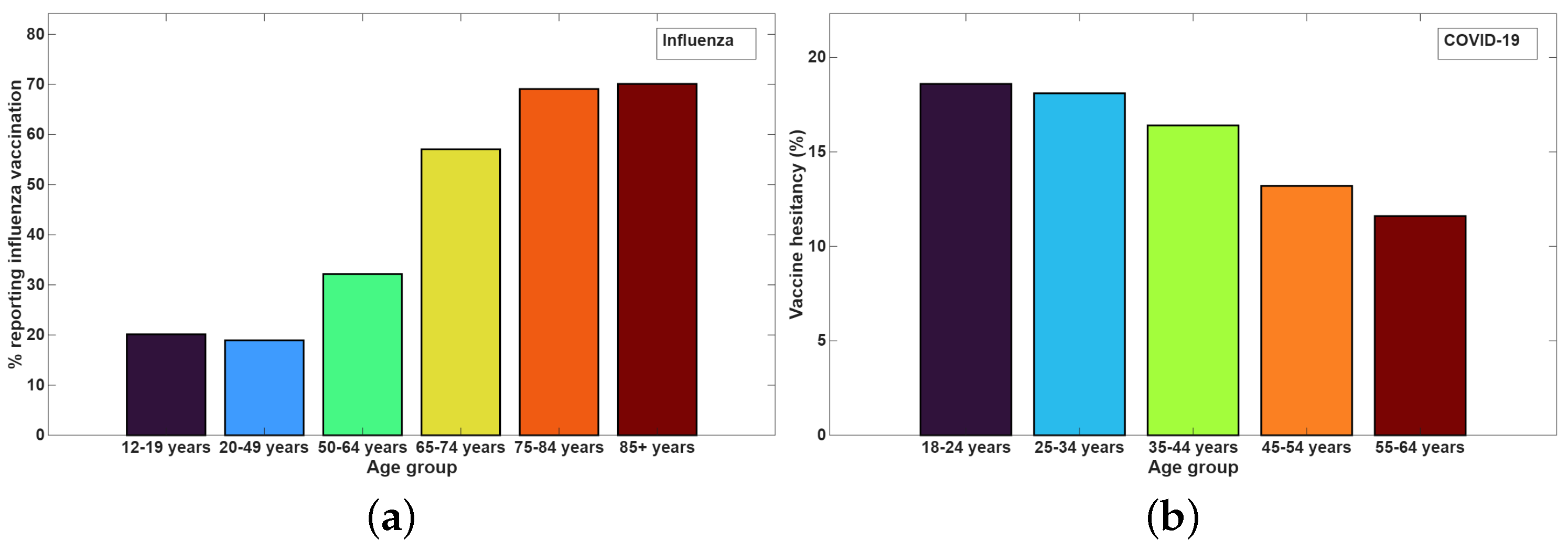
Figure 1. (a) Average percentage of individuals reporting influenza vaccination in different age groups in Canada (adapted from [53]); (b) Percentage of vaccine hesitancy in different age groups in the context of COVID-19 vaccine in France (adapted from [54]).
Mathematics 14 00162 g001
Figure 2. Plot of R 0 for different values of the disease duration τ . The blue curve corresponds to the Dirac delta distribution for the recovery and death rates, and the orange curve corresponds to the uniform distribution of recovery and death rates. The parameter values are β = 0.4 , ϵ = 0.9 , and ρ ^ 0 = 0.01 .
Mathematics 14 00162 g002
Figure 3. (a) Graphical representation of the memory kernels K t i m e ( ζ ) = a e a ζ , with a = 0.033 (green), a = 0.02 (blue), a = 0.014 (red) and K t i m e ( ζ ) = b d d b ( e b ζ e d ζ ) , with b = 0.033 ,   d = 0.05 (magenta); b = 0.02 ,   d = 0.05 (black). (b,c) show the corresponding plots of I ^ ( t ) and S ^ ( t ) , respectively. All other parameter values are given in the text. The arrows shown in the axis labels denote the direction of increase for the corresponding variables.
Mathematics 14 00162 g003
Figure 4. Impact of memory decay rate (a) and the vaccine effectiveness ( ϵ ) on the (a) maximum number of infected ( I ^ m ); (b) final size of epidemic ( S ^ f ) and (c) time to maximum infected ( t m ). The other parameter values are kept the same as mentioned in the text.
Mathematics 14 00162 g004
Figure 5. Impact of k and m 0 on the (a) maximum number of infected ( I ^ m ); (b) final size of epidemic ( S ^ f ) and (c) time to maximum infected ( t m ). The other parameter values are kept the same as mentioned in the text.
Mathematics 14 00162 g005
Figure 6. PRCC values of the parameters m 0 , k, ϵ and a on the model outcomes: (a) Maximum number of infected ( I ^ m ); (b) Final size of epidemic ( S ^ f ); (c) Time to maximum infected ( t m ).
Mathematics 14 00162 g006
Figure 7. Plot of the age-dependent parameters and initial conditions: (a) S 0 ( a ) , (b) I 0 ( a ) , (c) α ( a ) , (d) V ( a ) , (e) q ( a ) , (f) r 0 ( a ) , (g) d 0 ( t ) . The choices of these functions are taken from [58].
Mathematics 14 00162 g007aMathematics 14 00162 g007b
Figure 8. Plot of I ( a , t ) , ρ ( a , t ) involved in the age-dependent Model (6)–(8). (a) I ( a , t ) ; (b) ρ ( a , t ) . The parameter values are described in the text.
Mathematics 14 00162 g008
Figure 9. Impact of initial age-dependent distribution of susceptible population S 0 ( a ) . (a) Different age structures S 0 ( x ) . (b) I ^ ( t ) corresponding to the three cases in the left panel.
Mathematics 14 00162 g009
Figure 10. Plot of I ^ ( t ) for different choices of age-dependent memory kernel K ( a , t ) .
Mathematics 14 00162 g010
Figure 11. Reasons for vaccine hesitancy for COVID-19 vaccine.
Mathematics 14 00162 g011
Table 1. Description of parameters and variables used in the model.
Variable andDescriptionDimension
Parameter
S ( a , t ) Susceptible individuals of age a at time t P o p u l a t i o n
I ( a , t ) Infected individuals of age a at time t P o p u l a t i o n
R ( a , t ) Recovered individuals of age a at time t P o p u l a t i o n
D ( a , t ) Dead individuals of age a at time t P o p u l a t i o n
J ( a , t ) Newly infected individuals of age a at time t P o p u l a t i o n · t i m e 1
ρ ( a , t ) Proportion of vaccinated individuals of age a at time t D i m e n s i o n l e s s
r ( a , ξ ) Recovery rate distribution of age a at time since infection ξ t i m e 1
d ( a , ξ ) Death rate distribution of age a at time since infection ξ t i m e 1
α ( a ) Susceptibility rate at the age a V o l u m e · c o p i e s 1 · t i m e 1
V ( a ) Viral load at any time during the infectiousness period of an infected individual of age a C o p i e s · v o l u m e 1 · t i m e 1 · p o p u l a t i o n 1
ϵ Vaccine effectiveness D i m e n s i o n l e s s
A M Maximum possible age of an individual T i m e
P ( · ) Probability of vaccine uptake D i m e n s i o n l e s s
m ( a , t ) Information index in the age group a at time t D i m e n s i o n l e s s
Disclaimer/Publisher’s Note: The statements, opinions and data contained in all publications are solely those of the individual author(s) and contributor(s) and not of MDPI and/or the editor(s). MDPI and/or the editor(s) disclaim responsibility for any injury to people or property resulting from any ideas, methods, instructions or products referred to in the content.