Article

Benchmarking Adversarial Patch Selection and Location

Faculty of Electrical Engineering, Technion, Haifa 3200003, Israel
*
Author to whom correspondence should be addressed.
Mathematics 2026, 14(1), 103; https://doi.org/10.3390/math14010103 (registering DOI)
Submission received: 1 December 2025 / Revised: 21 December 2025 / Accepted: 25 December 2025 / Published: 27 December 2025
(This article belongs to the Special Issue AI Security and Edge Computing in Distributed Edge Systems)

Abstract

Adversarial patch attacks threaten the reliability of modern vision models. We present PatchMap, the first spatially exhaustive benchmark of patch placement, built by evaluating over 1.5 × 10 8 forward passes on ImageNet validation images. PatchMap reveals systematic “hot-spots” where small patches (as little as 2% of the image) induce confident misclassifications and large drops in model confidence. To demonstrate its utility, we propose a simple segmentation-guided placement heuristic that leverages off-the-shelf masks to identify vulnerable regions without any gradient queries. Across five architectures-including adversarially trained ResNet-50-our method boosts attack success rates by 8–13 percentage points compared to random or fixed placements.

1. Introduction

1.1. Background

Deep neural networks have achieved near-human accuracy on many vision benchmarks, yet they remain alarmingly brittle to small, localized perturbations. In particular, adversarial patches printed stickers or posters that can be physically applied to a scene have been shown to reliably fool classifiers and detectors in both digital and real-world settings [1,2,3]. Their practical threat spans self-driving cars, surveillance systems, and biometric authentication.
A patch attack is defined not only by what the patch looks like, but also by where it is placed. While there has been extensive work on crafting patch appearance (optimizing texture, shape, and color) [1,2], far less attention has been paid to the equally critical question of patch placement. In practice, many defenses and evaluation protocols implicitly assume a fixed placement (e.g., center or corner of the image), or optimize location jointly with texture on a limited number of examples [4,5]. At the same time, standardized resources such as ImageNet-Patch [6] provide transferable patch textures and have accelerated reproducible evaluation of patch content, but they do not characterize spatial vulnerability across the full range of possible locations.

1.2. Problem Statement and Gap

Without a systematic, large-scale study of patch placement, it is difficult to answer basic questions that directly affect both attack evaluation and defense design: Which regions of natural images are consistently most susceptible to small patches? How does vulnerability change with patch size? And how reliable are placement strategies that aim to approximate worst-case locations without costly model queries? Existing work provides only sparse evidence. Either by evaluating a small set of handpicked placements or by optimizing locations per image with limited coverage [4,5]. This leaves a gap: we lack a publicly available, spatially exhaustive benchmark that maps vulnerability as a function of location under controlled patch content, enabling fair comparison of placement strategies and revealing dataset-level “hot-spots”.

1.3. Motivation

Consider two identical patches: one pasted over a salient object region, the other over background. Intuitively, the former will more strongly disrupt classification, yet existing benchmarks provide only limited support for this intuition because they do not exhaustively probe placement. A comprehensive spatial analysis would quantify where patches are most harmful, how often strong effects occur, and whether simple, model-agnostic cues can reliably identify vulnerable locations.

1.4. PatchMap

We introduce PatchMap, a spatially exhaustive benchmark for adversarial patch placement built using transferable patch textures from ImageNet-Patch [6]. PatchMap v1 focuses on two representative, high-impact patches (IDs 2 and 6) and evaluates three square sizes (50, 25, 10 px) at every stride-2 location on a 2000-image subset of the ImageNet-1K validation set. This yields 1.5 × 10 8 forward passes on a standard ResNet-50, recording both predicted labels and softmax confidences at each location. The resulting dense “vulnerability maps” uncover stable hot-spots, quantify confidence collapse patterns, and expose spatial motifs that are invisible to sparse evaluations. The evaluation method is explained at Figure 1.

1.5. Contributions

  • PatchMap dataset. A public release of 100 M+ location-conditioned predictions at https://huggingface.co/datasets/PatchMap/PatchMap_v1 (accessed on 15 May 2025), scaling to 6.5 B entries.
  • Rigorous analysis. Unified definitions of attack-success rate (ASR) and confidence drop ( Δ conf ), evaluated across location, patch size, and model robustness, exposing recurring spatial vulnerabilities.
  • Segmentation-guided placement. A fast, zero-gradient heuristic that selects high-impact locations via off-the-shelf semantic masks, boosting ASR by 8–13 pp over random or fixed baselines-even on adversarially trained networks.
By decoupling what a patch looks like from where it lands, PatchMap lays the groundwork for location-aware defenses, adaptive attacks, and deeper insight into the spatial dynamics of adversarial vulnerability.

2. Related Work

2.1. Universal and Physical Adversarial Patches

Ref. [1] first introduced universal patches that consistently coerce a classifier into an attacker–chosen label. Because these patches are physically realizable, later studies printed them to fool real world systems: LaVAN places a small visible blob on the background [7], while RP2 stickers make stop signs read as speed limits [2]. Domain specific variants exist for face recognition, where perturbations are embedded in eyeglass frames [3], and for traffic sign detection [8]. The feasibility of such localized, robust attacks motivated datasets such as ImageNet-Patch [6], which supplies transferable patch textures later reused in our work.

2.2. Patch Placement and Location Optimisation

Early attacks fixed the patch at a predetermined corner or the object centre [2,7], implicitly assuming position mattered little. Subsequent research relaxed this by optimising location jointly with texture: LOAP employs gradient descent on both variables [4]; Simultaneous-Patch uses reinforcement learning (RL) to search position in a black-box setting [5]; PatchAttack learns an RL policy subject to a query budget [9]. Real-world “Adversarial Sticker” work further optimizes in-plane rotation and scale of printed patches [10]. Ref. [11] Examines patch placement selection on of street sign and the effect on object detection models. Generative Dynamic Patch Attack (GDPA) [12] a use GANs to propose both content and location, showing that placement is tightly coupled with texture generation. Attention-guided methods such as PS-GAN [13] infer high impact regions from saliency maps, while Shapeshifter extends the idea to object detection [2]. Despite this progress, prior studies either optimise on a handful of images or evaluate sparse locations; none offers an exhaustive, publicly released map of spatial vulnerability.

2.3. Context Awareness and Adaptive Attacks

Modern attacks adapt the patch to scene context. Distributed stickers cover multiple object parts for occlusion robustness [10], and Dynamic-Patch sequences adjust appearance over time [12]. Beyond classification, context-aware patches fool detectors, depth estimators, and segmentation networks, often by incorporating physical transforms (viewpoint, lighting) into training [2]. Several works exploit semantic priors: masking patches to background only, or using segmentation cues to stay off salient regions [14]. Our segmentation-guided heuristic takes the opposite tack-seeking the most segmentation-confident region-while remaining optimization-free and substantially faster than RL or gradient-based search. [15] explores leveraging of XAI such as Grad-CAM in order to select patch placement with an impact on model accuracy and that maintains difficulty to detect by the human eye.   PatchMap complements the above literature by offering the first large-scale, architecture-agnostic benchmark that decouples patch appearance from exhaustive placement, enabling quantitative comparison of any optimization-free or optimization-based strategy on common ground.
Adversarial attack methods are mostly compared using the ASR (Attack Success Rate) metric denoted as:
A S R = 1 N cc i = 1 N cc I y ^ y i ,
where y is the originally predicted ground truth, and y ^ is the prediction after the appliance of the attack. N cc is the number of correctly classified examples.

3. Dataset Design

3.1. Patch Source

We use the ten publicly released ImageNet-Patch adversaries of Li et al. [6]. Each 50 × 50 RGB patch is gradient–optimised for a distinct target class and shown to transfer across common CNN backbones. Fixing this set guarantees strict reproducibility and avoids the confound of re-optimising patch content. The patches are applied without rotation.

3.2. Spatial Sweep

For every ImageNet-1K validation image ( 224 × 224 ), each patch is pasted on a dense stride-2 grid of feasible centres. The grid contains 112 × 112 = 12,544 positions and is evaluated at three square sizes: native 50 × 50 , down-scaled 25 × 25 , and 10 × 10  px covering almost the whole image while keeping compute tractable. In total 50,000 images × 10 patches × 3 sizes × 12,544 locations 1.9 × 10 10 potential placements. By batching inference and discarding placements that would fall outside the frame, we actually run 1.1 × 10 8 forward passes-roughly two orders of magnitude more than any previous location study.

3.3. Model Attacked

All placements are evaluated on a standard ResNet-50 [16] from torchvision, pretrained on ImageNet and not adversarially fine-tuned. Future PatchMap releases will incorporate additional backbones, but v1.0 deliberately fixes a single architecture to keep the file size manageable.

3.4. Recorded Data Format

PatchMap is sharded: every triple (image_id, patch_id, patch_size) is stored in its .npy file named {img}_{patch}_{size}.npz. Each file contains a single NumPy array of shape 2 × 112 × 112 : the first slice holds the predicted class indices (int16); the second holds the corresponding soft-max confidences (float32). With 50 , 000 images, ten patches and three sizes, v1.0 comprises 1.5 million files totalling ∼1.5 GB after compression. This fine-grained layout lets users download only the subsets they need and stream batches directly from disk without monolithic archives.

3.5. Choice of Parameters

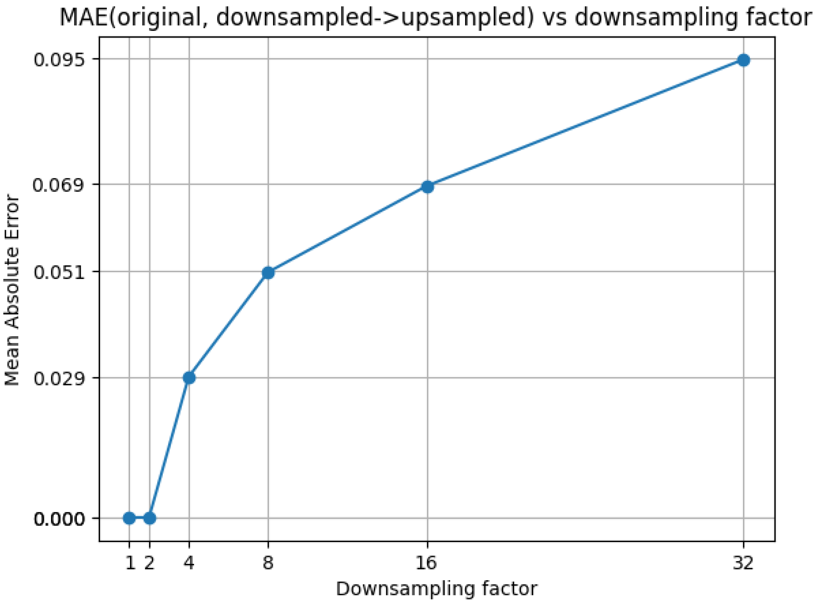
In choosing the parameters we performed an ablation study over 50 random images. We performed the evaluation on a 1-d stride and over all patches to select an optimal stride and optimal patches for the larger dataset. We perfomed the ablation over patches of size 50 × 50 . We chose a 2-stride grid for our dataset in comparison to the original image, as it yields identical results as for the full 1-stride grid, saving a significant amount of computations with no compromise in accuracy, as shown in Figure 2. The reason for that phenomenon is the architecture of resnet-50 containing a stride of 2 on the first convolution of the model. We chose patches 2 (“Plate”) and 6 (“Guitar”) as they have yielded better mean optimal ASR (as measured in Table 1) than any other patch on the same ablation case.

3.6. Resources

All benchmark evaluations can be performed with a single processor with at least 8 GB of memory (with/without GPU).

3.7. Public Release

PatchMap v1.0 (≈100 M predictions) is hosted on https://huggingface.co/datasets/PatchMap/PatchMap_v1 (accessed on 15 May 2025) HuggingFace under a CC-BY-4.0 license, bundled with loaders, plotting utilities, and a leaderboard script. A 6.5 B-entry v2.0, computed on a dedicated GPU cluster, will be released under the same terms. The code implementation of the project is available on https://github.com/PathMap7/PatchMap GitHub. (accessed on 15 May 2025, used branch master, commit 02bf1b9).

3.8. Why PatchMap?

Its exhaustive spatial coverage (covering a dense grid of all possible locations for path appliance, as explained in Section 3.2) allows researchers to map vulnerability hot-spots, train location-aware detectors, and benchmark placement strategies under identical conditions, and seek to obtain near-optimal results, instead of comparing to other methods. A comparison of PatchMap and other methods is provided in Table 2.

4. Evaluation Protocol

PatchMap’s dense annotations enable four complementary evaluations.
  • Location-wise attack-success heat-maps: For every grid cell ( k , l ) we compute the clean-correct attack-success rate
    ASR ( k , l ) = 1 N cc i = 1 N cc I y ^ i , k , l y i ,
    where N cc is the number of validation images that the model classifies correctly without a patch. The resulting 112 × 112 heat-map exposes systematic hot- and cold-spots.
  • Confidence and calibration shift: Besides logits, PatchMap records soft-max scores, enabling reliability analysis. We report (i) the average confidence drop Δ conf as detailed in (3). And (ii) the change in Expected Calibration Error (ECE) and Brier score between clean and patched images.
  • Size/conspicuity trade-off: Plotting ASR against patch area across the three sizes yields a Pareto curve that answers: How small can a patch be before its success drops below a chosen threshold?
  • Cross-model transfer: Given placements evaluated on model A, we re-score the exact locations on model B and assemble a transfer matrix T A B . Off-diagonal strength indicates universal spatial vulnerabilities; weak transfer suggests architecture-specific quirks.
  • Metrics are averaged over the full validation set and accompanied by 95 % bootstrap confidence intervals (1000 resamples). The public code reproduces every figure and table in under 2 GPU-hours on a single V100.
  • PatchMap therefore enables fine-grained, statistically sound evaluation of both attacks and defences, opening the door to location-aware robustness research.

5. Analysis and Findings

5.1. Attack-Success Rate (ASR)

For every image x i that the clean model classifies correctly, and for every patch location ( k , l ) , let y ˜ i , k , l denote the predicted label on the patched image x i M k , l and y ^ i the clean prediction. The location-wise ASR is then
ASR ( k , l ) = 1 N cc i = 1 N cc I y ˜ i , k , l y ^ i ,
where N cc is the number of clean-correct images.
Optimal location. For each image we also record the highest ASR over all positions; Table 3 reports the mean of this value across the dataset.
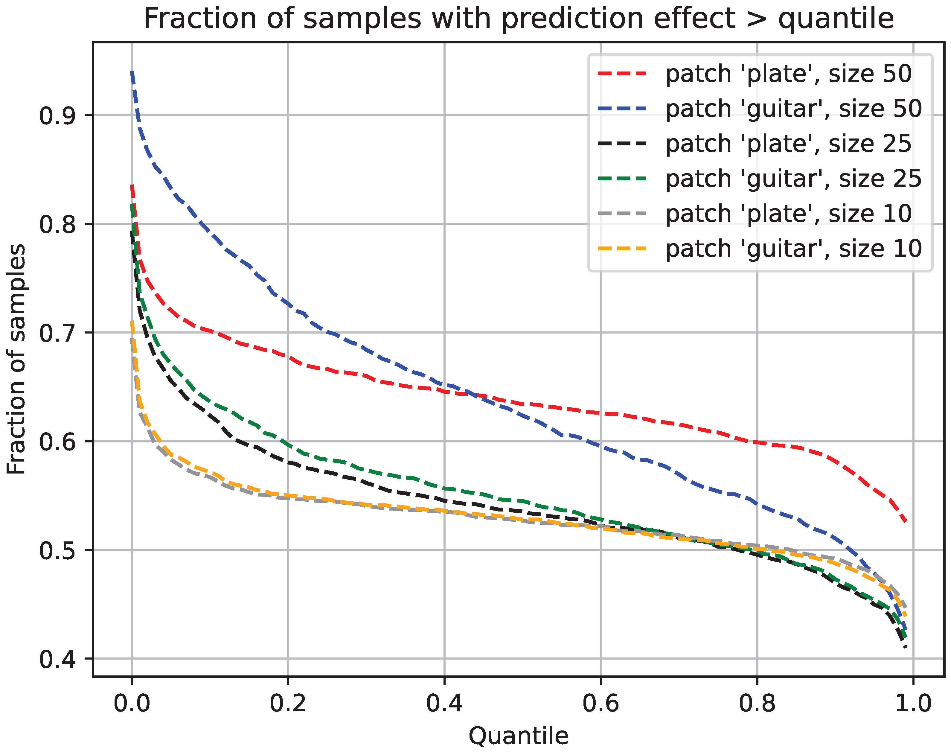
ASRq. Let w , h be the grid dimensions ( 112 × 112 ). ASR in quantile q measures the proportion of images fooled at at least a fraction q of all possible locations,
ASR q = 1 N cc i = 1 N cc I 1 w h k = 1 w l = 1 h [ y ˜ i , k , l y ^ i ] > q .
Figure 3 plots ASR q for two representative patches.

5.2. Confidence Effect

Let p θ ( y i x i ) be the clean soft-max confidence of the ground-truth class y i . The confidence drop for image i is the maximal change in the model achieved after the attack on any possible location:
Δ conf i = max k , l p θ ( y i x i ) p θ y i x i M k , l ,
i.e., the largest fall among all locations. Table 4 shows the mean Δ conf per patch size.
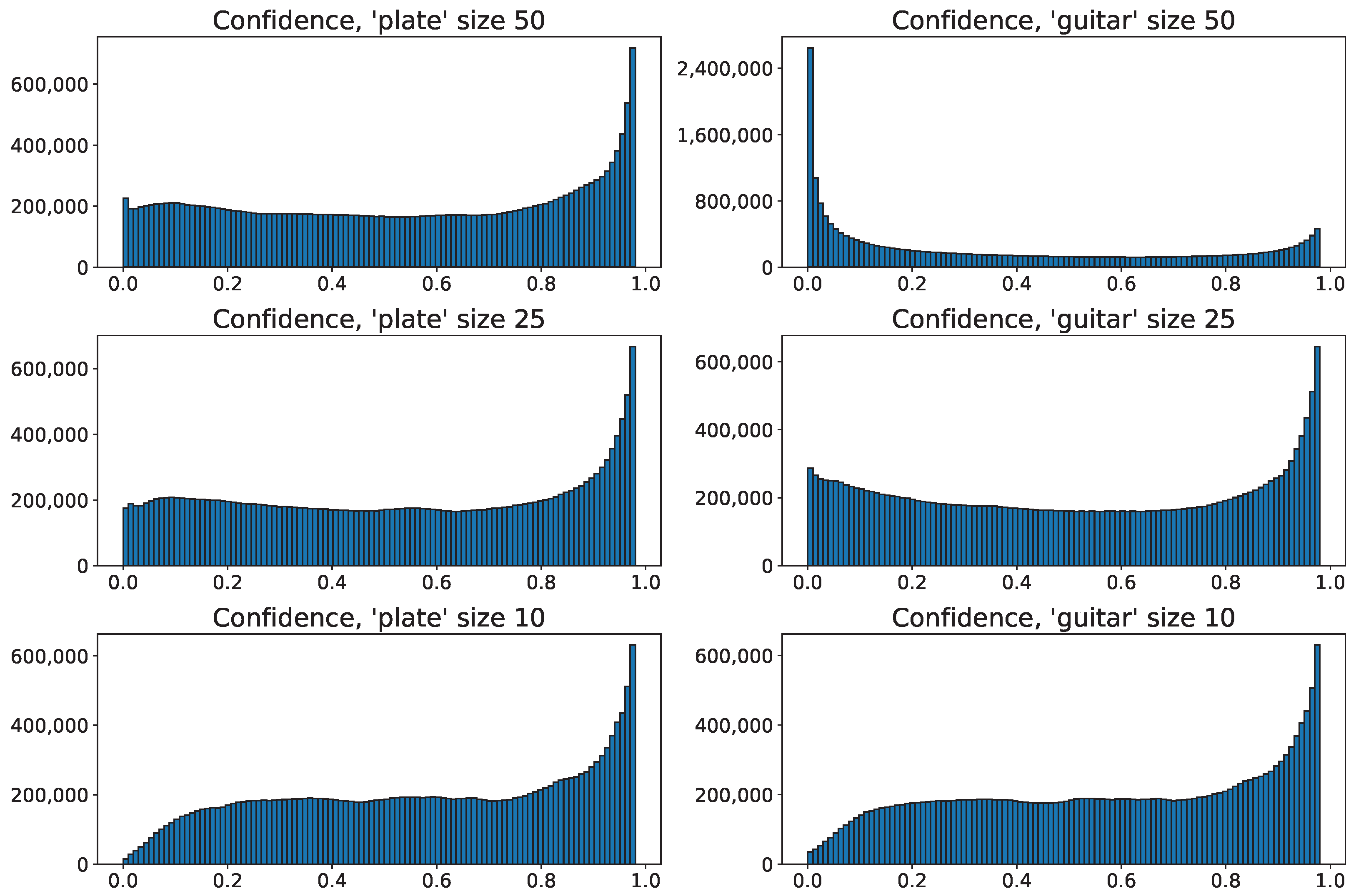
Figure 4 plots the distribution of post-attack confidences; larger patches incur heavier tails towards low confidence, with the “Guitar” patch producing the sharpest degradation at 50 × 50 .

6. Segmentation-Guided Patch Placement

6.1. Motivation

Most patch attacks search location by gradient descent or reinforcement learning-effective but slow and model-dependent. We observe that semantic-segmentation networks already highlight the pixels most critical for recognizing objects. If a patch occludes those pixels, it should hurt the classifier without any extra optimization. We therefore use segmentation confidence as a fast, architecture-agnostic cue for placing the patch, that proven to be valid when trained on sufficient amount of data [17], despite their limitations [18].

6.2. Approach

Let g ( x ) [ 0 , 1 ] H × W × C be per-pixel soft-max scores from a segmentation model, where channel b is background. Define the object-confidence map
S = 1 g ( x ) b .
Given a binary patch mask M { 0 , 1 } s × s , we slide M over S and pick the location that maximises the summed confidence it covers:
( k , l ) = arg max k , l S Shift k , l ( M ) 1 ,
where ⊙ is the element-wise product, Shift k , l centres the mask at ( k , l ) , and ( · ) 1 sums all entries. The chosen centre ( k , l ) is used for every tested classifier; no gradients or queries to the attacked model are required.
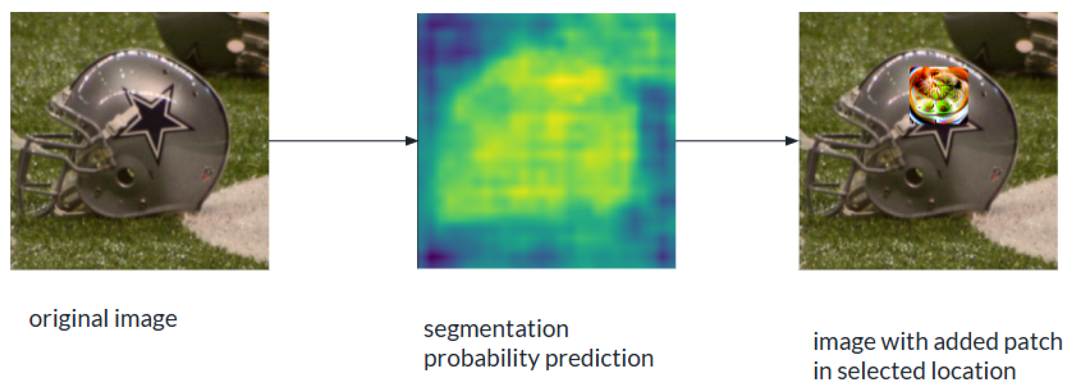
The method is demonstrated in Figure 5.

6.3. Experimental Setup

We evaluate all placement strategies on the ImageNet-1K validation split, resizing each image to 224 × 224 pixels. Five classifiers are attacked: ResNet-18 [16], ResNet-50, MobileNet-V2 [19], EfficientNet-B1 [20], Zero-Shot CLIP [21], and a Fast Adversarially Trained ResNet-50 [22]. Patch placement is guided by DeepLab-v3+ [23] with a ResNet-101 backbone, pretrained on PASCAL-VOC 2012, whose segmentation confidences serve as a zero-gradient cue. All experiments can be conducted with a single processor with at least 8 GB of memory (with/without GPU).
Unless stated otherwise, the adversary is the “Plate” universal patch from ImageNet-Patch [6], resized to 50 × 50 (≈4.98% of the image) and without rotation. We benchmark three optimisation-free placement rules: (i) Random-uniformly sampling the patch centre, (ii) Fixed-choosing the best of four preset offsets from the image centre, and (iii) our Seg-guided heuristic described in (4).
Performance is reported as attack-success rate (ASR) on the subset of images that each model classifies correctly in the clean setting.

6.4. Overall Performance

Table 5 compares attack-success rates (ASR) for three optimisation-free placement strategies. Across all four ImageNet-trained architectures, the segmentation-guided (Seg-guided) heuristic achieves the highest ASR, improving on Random placement by an average of 8 pp and outperforming the Fixed four-offset baseline by 13 pp. Crucially, the advantage persists on the adversarially trained ResNet-50, where Seg-guided placement still raises ASR from 0.31–0.36 to 0.39, underscoring that robust training alone is not sufficient to counter strategic patch positioning. Table 6 compares the average confidence drop Δ conf for one patch of sizes 25 × 25 , 50 × 50 and one model.

6.5. Effect of Patch Size

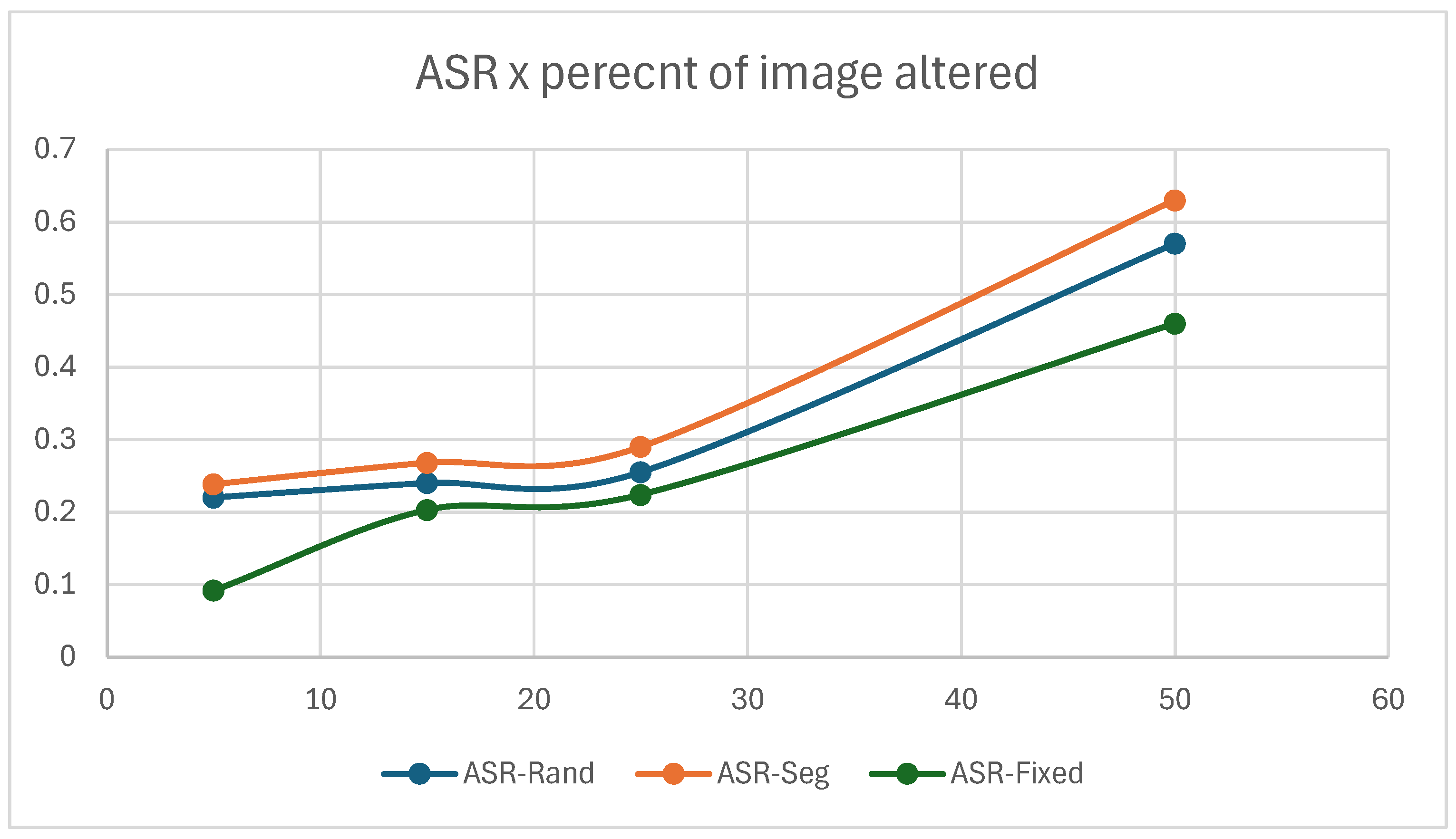
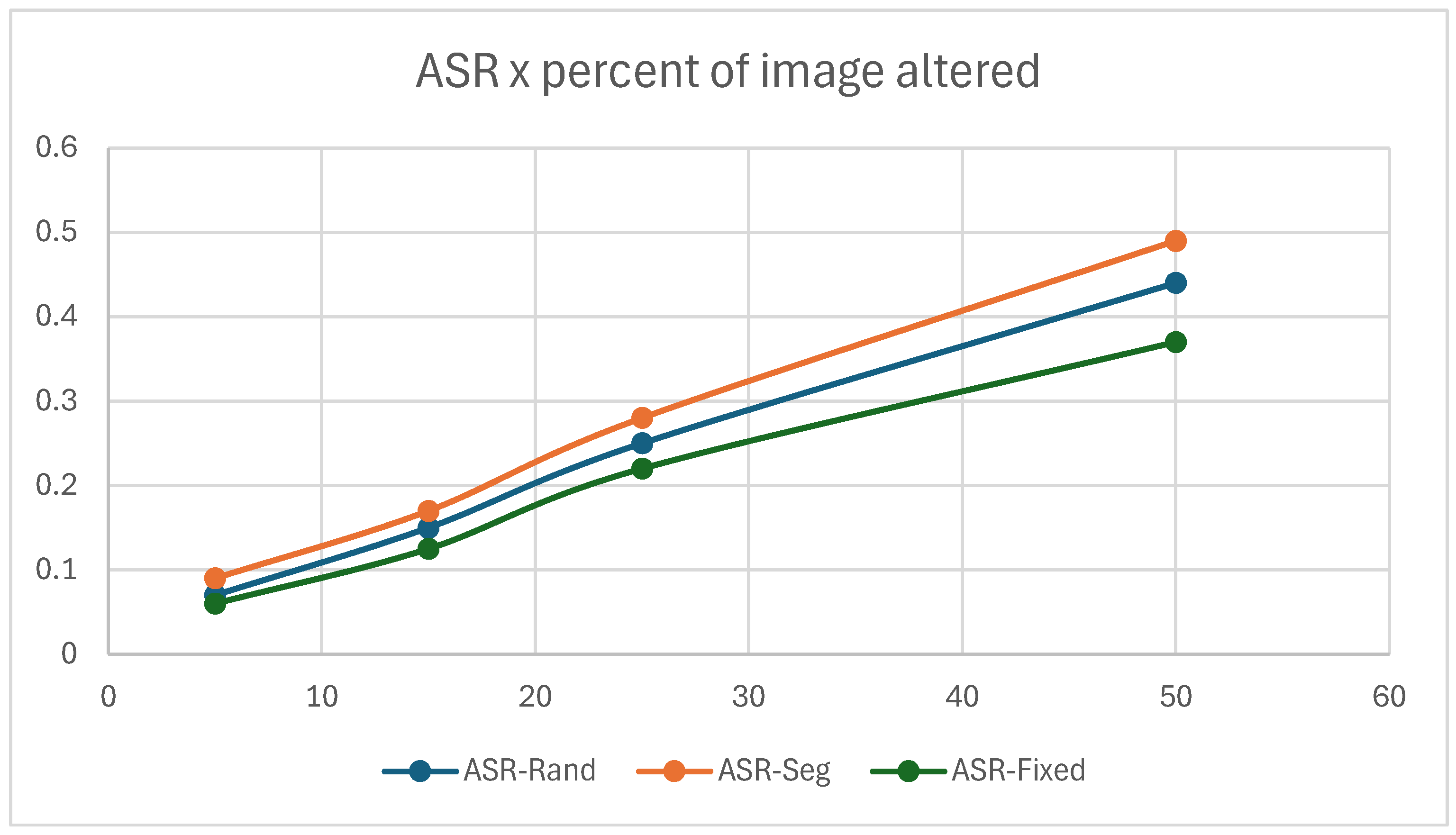
Figure 6, Figure 7 and Figure 8 plots ASR against patch side length on a representative ResNet-18 for lengths { 5 , 15 , 25 , 50 } . All methods degrade as the patch shrinks, yet Seg-guided placement maintains a consistent margin: with a 10 × 10 px patch-covering barely 2% of the image-it still fools 27% of clean-correct samples, versus 18% for Random and 14 % for Fixed. This resilience indicates that the segmentation heat-map is a reliable cue even when the patch is almost imperceptible.

6.6. Correlation with Confidence Drop

We examine how segmentation confidence predicts the eventual confidence drop of the classifier at each location. Define overall object confidence
p seg ( object x ) = 1 g ( x ) b
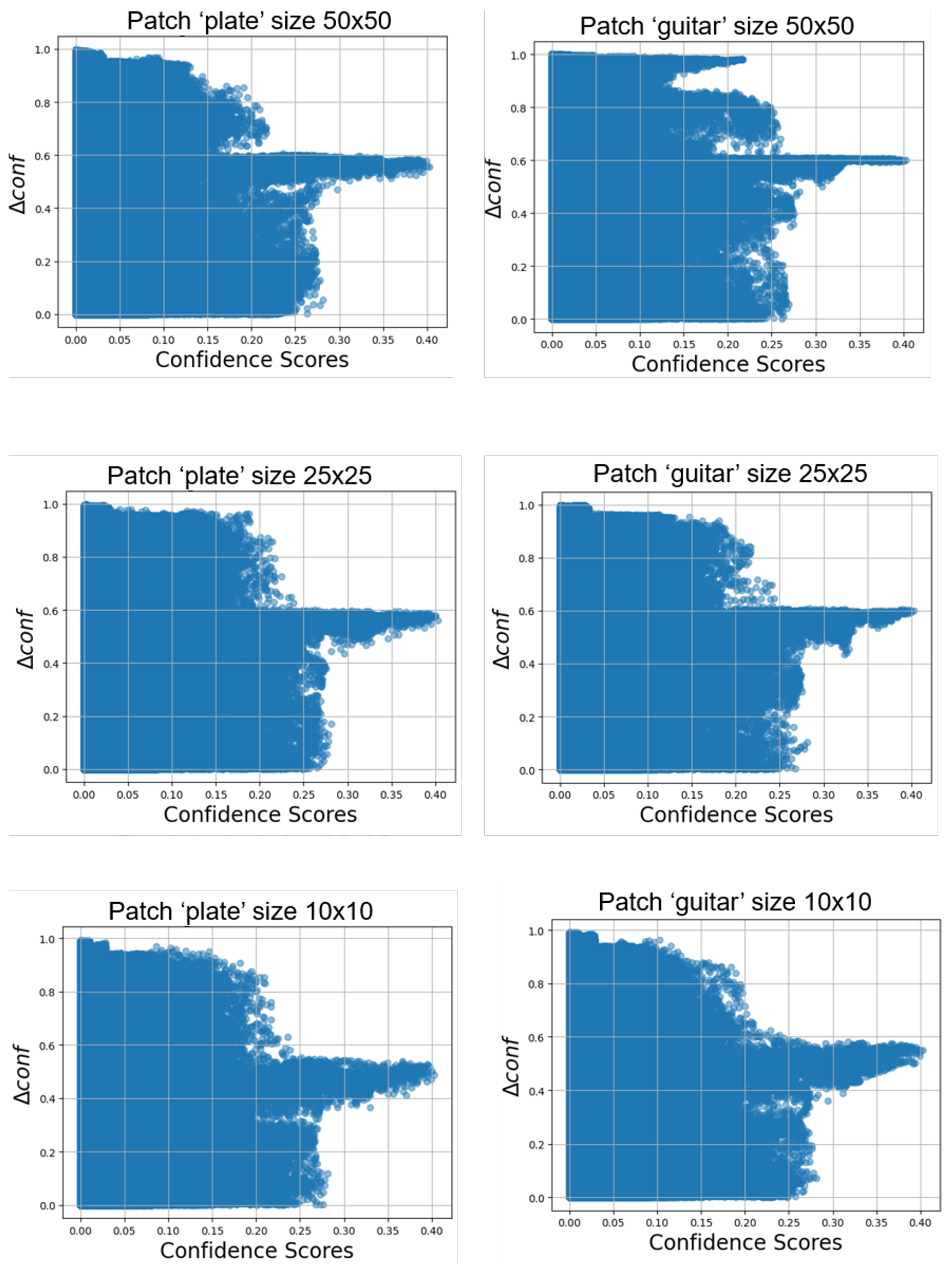
cf. Equation (5). Figure 9 examines the correlation between segmentation confidence (as detailed previously) and the effect on the ground-truth class confidence Δ conf for several possible patches. There is a strong correlation for scores above 0.2, especially for smaller patches, confirming that the segmentation map is a useful but not perfect proxy for the worst-case location. A possible explanation for that phenomenon is that lower confidence effect of the patch is obtained due to the addition of a new object to the image (the adversarial patch), and not by changing the object itself. Thus, in certain areas of the image, the object is covered by an adversarial patch which makes no further effect than a patch besides the object.

6.7. Qualative Examples

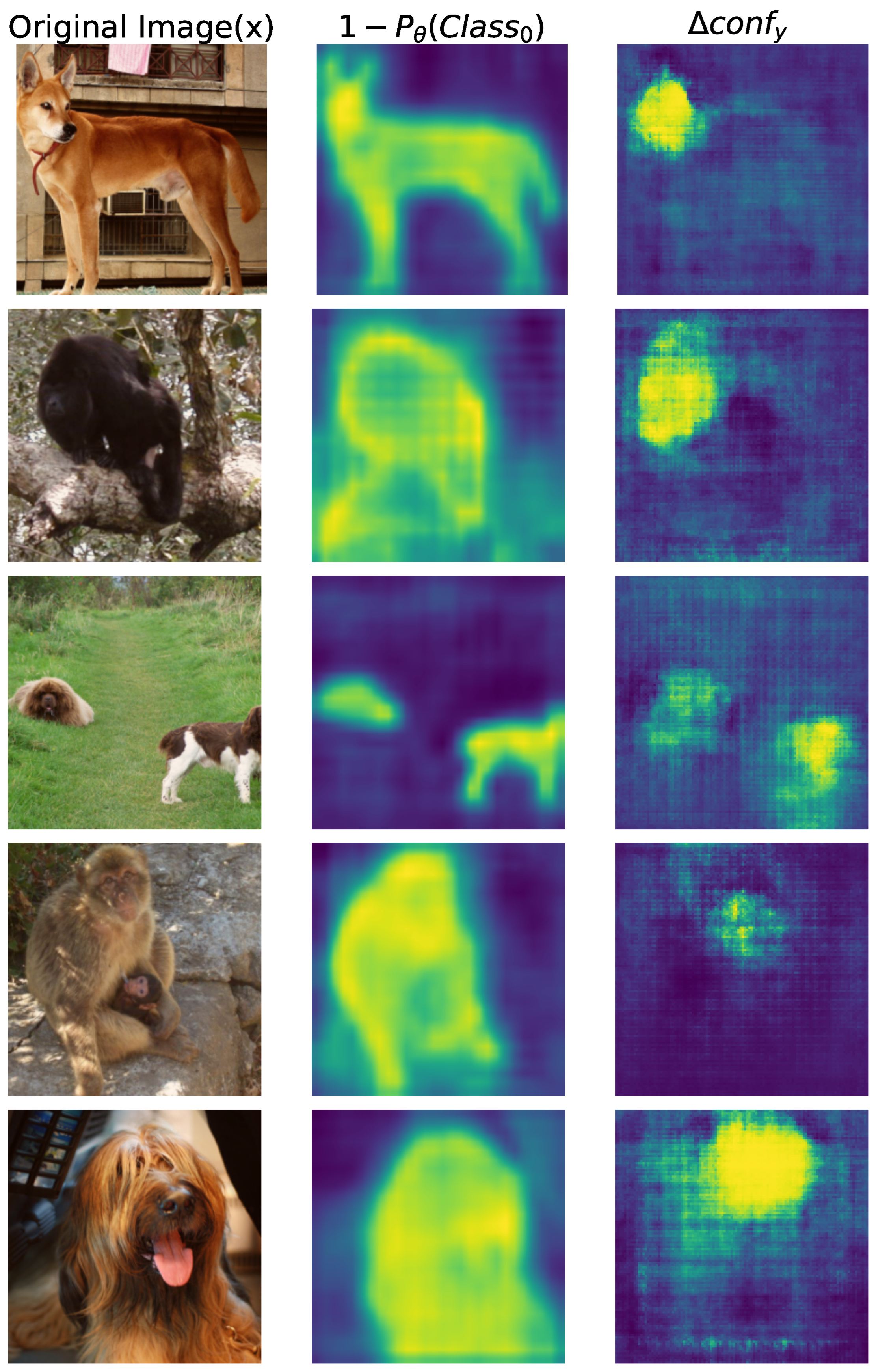
Figure 10 demonstrates the connection between the segmentation probability prediction by DeepLabV3Plus with a Resnet-101 backbone as detailed in Section 6.3 as not object (i.e., 1 P θ ( c l a s s 0 ) where c l a s s 0 is background), and the empirical map of Δ c o n f y i.e., the effect on the prediction probability of the ground-truth class y measured on ResNet-18, after appliance of patch “Plate” of size 50 × 50 . Most locations which yield the highest effect are indeed part of the predicted object, much of the predicted object is does not yield the highest Δ conf values.
For large objects, there are distinctive parts that define the object (For example, the head of a dog is important in defining and identifying that it is indeed a dog), these areas show a higher value of Δ c o n f y meaning that these areas are more vulnerable to patch placement. Compared to other placement methods such as in [11] prioritizing path placement on the object, they like our method miss the optimal patch placement in a significant portion of the images.

7. Conclusions

We have introduced PatchMap, the first large-scale, spatially exhaustive benchmark for adversarial patch placement. By evaluating over 1.0 × 10 8 patch placements on ImageNet–1K validation images, PatchMap uncovers consistent “hot-spots” of vulnerability and quantifies how attack success and confidence collapse vary across both location and patch size.
Building on this dataset, we proposed a simple, segmentation-guided placement heuristic that leverages off-the-shelf semantic masks to select high-impact regions without any gradient queries or fine-tuning of the target model. Across five architectures-including adversarially trained ResNet-50-our method yields an 8–13 pp improvement in attack-success rate over random or fixed baselines, demonstrating that zero-gradient spatial cues can substantially amplify patch efficacy.
Looking forward, PatchMap opens the door to a new class of location-aware defenses and attacks, allowing for methods to find the optimal patch location with respect to universal patch attack, in new domains such as medical [24] or robotics [25]. Other direction is to understand the relation between input patch attacks and bit-flip attacks [26], as those are the most practical in real world setup.
Future releases (v2.0) will scale to 6.5 billion placements and incorporate diverse backbones (ViT, ConvNeXt and modified architectures [27]), enabling cross-family transfer studies. We anticipate that researchers will build on PatchMap to design spatially informed detectors, robust training curricula, and context-dependent attacks across classification, detection, and beyond, advancing the security and reliability of vision systems.

7.1. Task Scope

Our benchmark focuses on ImageNet-style image classification. Extending PatchMap to detection and segmentation is non-trivial, since patch placement interacts with multi-instance scenes, localization objectives, and different evaluation metrics (mAP/IoU). We view this as an important direction for future releases.

7.2. Segmentation Prior

Our segmentation guided placement uses a single pretrained segmentation model (DeepLab-v3) trained on PASCAL-VOC. While this choice keeps the method simple and reproducible, the strength of the placement signal may vary across segmentation backbones, training datasets, and newer foundation segmentation models.

7.3. Patch Transforms and Physical Realism

PatchMap v1 uses static, axis aligned square patches without rotation. This setting is sufficient to reveal systematic spatial hot-spots, but it does not capture physical effects such as rotation, perspective deformation or illumination changes. Incorporating these transforms would enable more realistic benchmarking of physical-world attacks.

Author Contributions

Conceptualization, M.K.; Methodology, S.K.; Software, S.K.; Formal analysis, S.K.; Investigation, M.K.; Writing—original draft, S.K.; Writing—review & editing, M.K. and A.M.; Visualization, S.K.; Supervision, A.M.; Project administration, A.M. All authors have read and agreed to the published version of the manuscript.

Funding

This research received no external funding.

Data Availability Statement

The data presented in this study are openly available in PatchMap at https://huggingface.co/PatchMap/datasets (accessed on 15 May 2025).

Conflicts of Interest

The authors declare no conflict of interest.

References

  1. Brown, T.B.; Mane, D.; Roy, A.; Abadi, M.; Gilmer, J. Adversarial Patch. arXiv 2017, arXiv:1712.09665. [Google Scholar]
  2. Eykholt, K.; Evtimov, I.; Fernandes, E.; Li, B.; Rahmati, A.; Xiao, C.; Prakash, A.; Kohno, T.; Song, D. Robust Physical-World Attacks on Deep Learning Visual Classification. In Proceedings of the IEEE Conference on Computer Vision and Pattern Recognition (CVPR), Salt Lake City, UT, USA, 18–22 June 2018; pp. 1625–1634. [Google Scholar]
  3. Sharif, M.; Bhagavatula, S.; Bauer, L.; Reiter, M.K. Accessorize to a Crime: Real and Stealthy Attacks on State-of-the-Art Face Recognition. In Proceedings of the ACM Conference on Computer and Communications Security (CCS), Vienna, Austria, 24–28 October 2016; ACM: New York, NY, USA, 2016; pp. 1528–1540. [Google Scholar]
  4. Rao, S.; Stutz, D.; Schiele, B. Adversarial Training Against Location-Optimized Adversarial Patches. In Proceedings of the European Conference on Computer Vision (ECCV) Workshops, Glasgow, UK (Virtual Event), 23–28 August 2020. [Google Scholar]
  5. Wei, X.; Guo, Y.; Yu, J.; Zhang, B. Simultaneously Optimizing Perturbations and Positions for Black-Box Adversarial Patch Attacks. IEEE Trans. Pattern Anal. Mach. Intell. 2023, 45, 9041–9054. [Google Scholar] [CrossRef] [PubMed]
  6. Li, X.; Yin, X.; Chuang, S.; van der Maaten, L.; Hadsell, R.; Feichtenhofer, C. ImageNet-Patch: A Dataset for Benchmarking Adversarial Patch Robustness in Image Classification. arXiv 2022, arXiv:2205.08649. [Google Scholar]
  7. Karmon, D.; Zoran, D.; Goldberg, Y. LaVAN: Localized and Visible Adversarial Noise. In Proceedings of the 35th International Conference on Machine Learning (ICML), Stockholmsmässan, Stockholm, Sweden, 10–15 July 2018; Dy, J., Krause, A., Eds.; Proceedings of Machine Learning Research. PMLR: Cambridge, MA, USA, 2018; Volume 80, pp. 2507–2515. [Google Scholar]
  8. Tsuruoka, G.; Sato, T.; Chen, Q.A.; Nomoto, K.; Kobayashi, R.; Tanaka, Y.; Mori, T. Adversarial Retroreflective Patches: A Novel Stealthy Attack on Traffic Sign Recognition at Night. In Proceedings of the VehicleSec 2024: Symposium on Vehicle Security and Privacy (Poster/WIP), San Diego, CA, USA, 26 February 2024. [Google Scholar] [CrossRef]
  9. Yang, C.; Kortylewski, A.; Xie, C.; Cao, Y.; Yuille, A. PatchAttack: A Black-box Texture-based Attack with Reinforcement Learning. In Proceedings of the European Conference on Computer Vision (ECCV), Glasgow, UK (Virtual Event), 23–28 August 2020. [Google Scholar]
  10. Wei, X.; Guo, Y.; Yu, J. Adversarial Sticker: A Stealthy Attack Method in the Physical World. IEEE Trans. Pattern Anal. Mach. Intell. 2023, 45, 2711–2725. [Google Scholar] [CrossRef] [PubMed]
  11. Hingun, N.; Sitawarin, C.; Li, J.; Wagner, D. REAP: A Large-Scale Realistic Adversarial Patch Benchmark. In Proceedings of the IEEE/CVF International Conference on Computer Vision (ICCV), Paris, France, 2–6 October 2023; pp. 4640–4650. [Google Scholar] [CrossRef]
  12. Li, X.; Ji, S. Generative Dynamic Patch Attack. In Proceedings of the British Machine Vision Conference (BMVC), Online, 22–25 November 2021. [Google Scholar]
  13. Liu, A.; Liu, X.; Fan, J.; Ma, Y.; Zhang, A.; Xie, H.; Tao, D. Perceptual-Sensitive GAN for Generating Adversarial Patches. In Proceedings of the AAAI Conference on Artificial Intelligence, Honolulu, HI, USA, 27 January–1 February 2019. [Google Scholar]
  14. Luo, J.; Bai, T.; Zhao, J. Generating Adversarial yet Inconspicuous Patches with a Single Image. In Proceedings of the Thirty-Fifth AAAI Conference on Artificial Intelligence (AAAI-21) Student Abstract and Poster Program, Virtual Event, 2–9 February 2021; pp. 15837–15838. [Google Scholar] [CrossRef]
  15. Lee, H.J.; Kim, J.S.; Lee, H.J.; Choi, S.H. POSES: Patch Optimization Strategies for Efficiency and Stealthiness Using eXplainable AI. IEEE Access 2025, 13, 57166–57176. [Google Scholar] [CrossRef]
  16. He, K.; Zhang, X.; Ren, S.; Sun, J. Deep Residual Learning for Image Recognition. arXiv 2015, arXiv:1512.03385. [Google Scholar] [CrossRef]
  17. Kimhi, M.; Kimhi, S.; Zheltonozhskii, E.; Litany, O.; Baskin, C. Semi-Supervised Semantic Segmentation via Marginal Contextual Information. arXiv 2024, arXiv:2308.13900. [Google Scholar] [CrossRef]
  18. Kimhi, M.; Kerem, O.; Grad, E.; Rivlin, E.; Baskin, C. Noisy Annotations in Semantic Segmentation. arXiv 2024, arXiv:2406.10891. [Google Scholar]
  19. Sandler, M.; Howard, A.; Zhu, M.; Zhmoginov, A.; Chen, L.C. MobileNetV2: Inverted Residuals and Linear Bottlenecks. In Proceedings of the IEEE/CVF Conference on Computer Vision and Pattern Recognition (CVPR), Salt Lake City, UT, USA, 18–22 June 2018; pp. 4510–4520. [Google Scholar] [CrossRef]
  20. Tan, M.; Le, Q.V. EfficientNet: Rethinking Model Scaling for Convolutional Neural Networks. In Proceedings of the 36th International Conference on Machine Learning, Long Beach, CA, USA, 9–15 June 2019; Proceedings of Machine Learning Research. PMLR: Cambridge, MA, USA, 2019; Volume 97, pp. 6105–6114. [Google Scholar]
  21. Radford, A.; Kim, J.W.; Hallacy, C.; Ramesh, A.; Goh, G.; Agarwal, S.; Sastry, G.; Askell, A.; Mishkin, P.; Clark, J.; et al. Learning Transferable Visual Models from Natural Language Supervision. arXiv 2021, arXiv:2103.00020. [Google Scholar] [CrossRef]
  22. Wong, E.; Rice, L.; Kolter, J.Z. Fast is better than free: Revisiting adversarial training. In Proceedings of the International Conference on Learning Representations (ICLR), Addis Ababa, Ethiopia (Virtual Event), 26–30 April 2020. [Google Scholar]
  23. Chen, L.C.; Zhu, Y.; Papandreou, G.; Schroff, F.; Adam, H. Encoder-Decoder with Atrous Separable Convolution for Semantic Image Segmentation. In Proceedings of the Computer Vision–ECCV 2018, Munich, Germany, 8–14 September 2018; Lecture Notes in Computer Science. Springer: Berlin/Heidelberg, Germany, 2018; Volume 11211, pp. 833–851. [Google Scholar] [CrossRef]
  24. Ronneberger, O.; Fischer, P.; Brox, T. U-Net: Convolutional Networks for Biomedical Image Segmentation. arXiv 2015, arXiv:1505.04597. [Google Scholar] [CrossRef]
  25. Kimhi, M.; Vainshtein, D.; Baskin, C.; Di Castro, D. Robot instance segmentation with few annotations for grasping. In Proceedings of the 2025 IEEE/CVF Winter Conference on Applications of Computer Vision (WACV), Tucson, AZ, USA, 28 February–4 March 2025; pp. 7939–7949. [Google Scholar]
  26. Galil, I.; Kimhi, M.; El-Yaniv, R. No Data, No Optimization: A Lightweight Method to Disrupt Neural Networks with Sign-Flips. arXiv 2025, arXiv:2502.07408. [Google Scholar] [CrossRef]
  27. Kimhi, M.; Kashani, I.; Mendelson, A.; Baskin, C. Hysteresis Activation Function for Efficient Inference. In Proceedings of the 4th NeurIPS Efficient Natural Language and Speech Processing Workshop, Vancouver, BC, Canada, 14 December 2024. [Google Scholar]
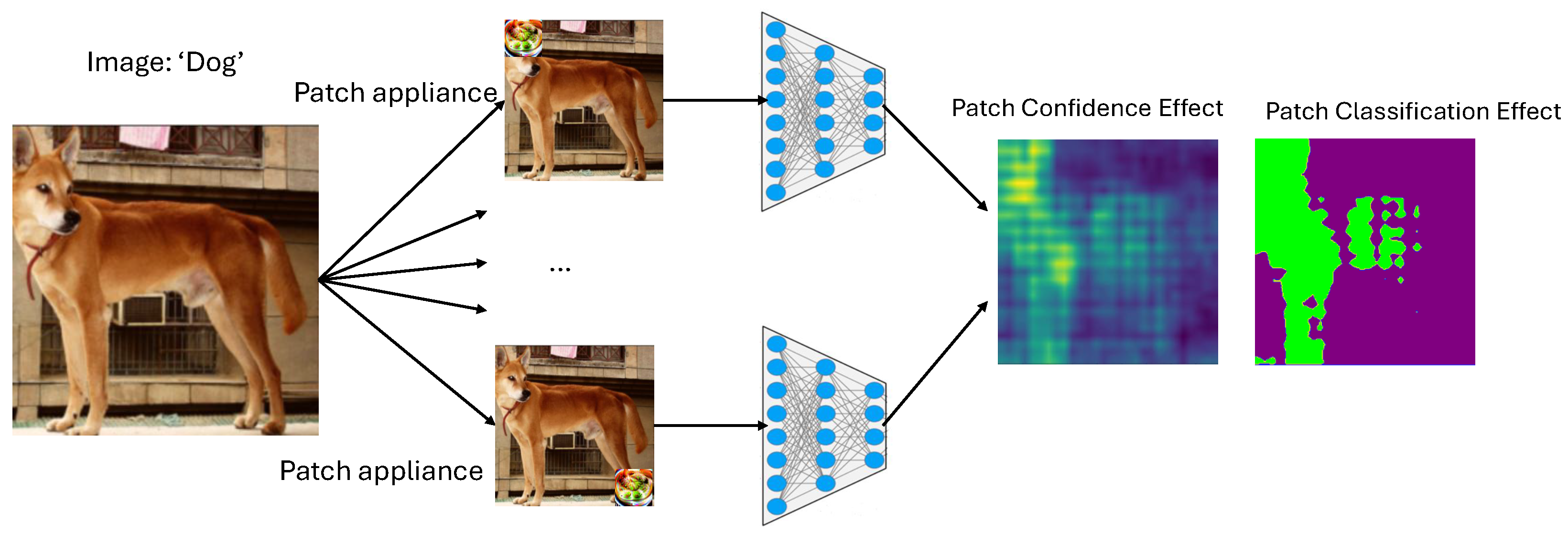
Figure 1. PatchMap evaluation method: We apply patch for any location in the image, and for each location we estimate the predicted class of the model and the confidence of the model on the ground truth class (y).
Mathematics 14 00103 g001
Figure 2. Ablation of the MAE (Mean Absolute error) of the confidence per mask between the 1-stride mask an x-stride mask. Blue dots represent sample values.
Mathematics 14 00103 g002
Figure 3. ASR q (2): fraction of images misclassified at more than a q-portion of locations. A S R q indicates the robustness of the effect of the patch on the model with respect to the location of the patch in the image. Patch “Plate” of size 50 × 50 is the most robust in that sense, as effect is least effected by location obtaining the best results for the worst 60 % of patch locations, “Guitar” of size 50 × 50 obtains the best results for ≈40% of the best patch locations.
Mathematics 14 00103 g003
Figure 4. Histogram of soft-max confidence on the ground-truth class after patching.
Mathematics 14 00103 g004
Figure 5. Pipeline of the segmentation-guided placement. A segmentation heat-map (middle) guides the patch (right) to the most confident object region. Colors: blue-green spectrum from low-high values.
Mathematics 14 00103 g005
Figure 6. ASR on ResNet-18 versus patch size for patch ‘Plate’.
Mathematics 14 00103 g006
Figure 7. ASR on ResNet-18 versus patch size for patch ‘Typewriter’.
Mathematics 14 00103 g007
Figure 8. ASR on ResNet-18 versus patch size for patch ‘Electric Guitar’. Optimal placement remains crucial as size shrinks.
Mathematics 14 00103 g008
Figure 9. Correlation between segmentation confidence and classifier confidence drop ( Δ conf ).
Mathematics 14 00103 g009
Figure 10. Left to Right: Original Image, Segmentation confidence prediction, Predicted confidence drop map, each pixel represents the confidence when the adversarial patch is applied at that location.
Mathematics 14 00103 g010
Table 1. Ablation: mean optimal ASR: fraction of images for which some location causes a misclassification. Patches 2 and 6 yields better optimal location, allowing for a higher attack success rate on an optimal patch placement location. In bold are the top-2 highest A S R patches.
Patch SizePatch
Patch 0 (“Soap Dispenser”)0.82
Patch 1 (“Cornet”)0.78
Patch 2 (“Plate”)0.84
Patch 3 (“Banana”)0.78
Patch 4 (“Cup”)0.78
Patch 5 (“Typewriter”)0.83
Patch 6 (“Guitar”)0.94
Patch 7 (“Hair Spray”)0.80
Patch 8 (“Sock”)0.76
Patch 9 (“Cellphone”)0.76
Table 2. Comparison of public adversarial-patch benchmarks. ✓ yes, × no.
BenchmarkTaskl#Imgs#PatchesSizesLoc/img#EvalsExhLocCached
ImageNet-Patch [6]Cls50 k101 ( 50 × 50 px)1 50 k××
REAP [11]Det84333 14,651××
PatchMap (v1, ours)Cls2 k2 (IDs 2,6)3 (10/25/50 px)12,544150.5 M
One placement per sample with random affine (translation/rotation); no dense per-location map. Small/medium/large physical patch sizes (e.g., 10″ × 10″, 10″ × 20″, two 10″ × 20″), rendered with per-sign geometric + lighting transforms. 2000 × 2 × 3 × ( 112 × 112 ) = 150,528,000 placements (stride-2 grid on 224 × 224 ). Cached = released precomputed per-location model outputs/maps (rather than only images/transforms). # represents number of.
Table 3. Mean optimal ASR: fraction of images for which some location causes misclassification.
Patch SizePatch 2 (“Plate”)Patch 6 (“Guitar”)
50 × 50 0.840.94
25 × 25 0.790.82
10 × 10 0.690.71
Table 4. Average confidence drop Δ conf at the worst location per image.
Patch SizePatch 2Patch 6
50 × 50 0.620.71
25 × 25 0.600.62
10 × 10 0.450.48
Table 5. ASR of optimisation-free placement strategies. Patch resized with no rotation. Bold: the optimal result for each setup.
ModelRandomFixedSeg-Guided
Plate 50 × 50 ( 4.98%)
Improvement 0.052
ResNet-500.390.320.46
+ Adverserial Training [22]0.360.310.39
ResNet-180.570.460.63
MobileNet-V20.480.410.55
EfficientNet-B10.380.340.42
CLIP0.440.430.47
Plate 25 × 25 ( 1.25%)
Average Improvement 0.042
ResNet-500.190.150.21
+ Adverserial Training [22]0.110.090.14
ResNet-180.220.250.29
MobileNet-V20.350.320.37
CLIP0.370.350.43
Electirc Guitar 50 × 50 ( 4.98%)
Average Improvement 0.046
ResNet-500.320.270.36
+ Adverserial Training [22]0.240.170.3
ResNet-180.440.370.49
MobileNet-V20.480.420.52
CLIP0.390.300.43
Electirc Guitar 25 × 25 ( 1.25%)
Average Improvement 0.030
ResNet-500.190.160.22
+ Adverserial Training [22]0.090.070.12
ResNet-180.250.220.28
MobileNet-V20.330.310.36
CLIP0.370.320.41
Typewriter Keyboard 50 × 50 ( 4.98%)
Average Improvement 0.058
ResNet-500.330.280.37
+ Adverserial Training [22]0.210.140.26
ResNet-180.430.370.48
MobileNet-V20.470.420.52
CLIP0.380.310.41
Typewrtier Keyboard 25 × 25 ( 1.25%)
Average Improvement 0.024
ResNet-500.180.150.20
+ Adverserial Training [22]0.100.070.12
ResNet-180.230.190.25
MobileNet-V20.330.310.35
CLIP0.350.280.39
Table 6. Δ conf of optimisation-free placement strategies on ResNet-50. Patch resized with no rotation. Bold: the optimal result for each setup.
PatchSizeRandomFixedSeg-Guided
Plate 50 × 50 0.630.520.69
Plate 25 × 25 0.380.320.42
Disclaimer/Publisher’s Note: The statements, opinions and data contained in all publications are solely those of the individual author(s) and contributor(s) and not of MDPI and/or the editor(s). MDPI and/or the editor(s) disclaim responsibility for any injury to people or property resulting from any ideas, methods, instructions or products referred to in the content.