
Network Optimization of Fresh Products Cold Chain Considering Supply Disruption and Demand Fluctuation Under the Dual-Carbon Policy

Abstract
1. Introduction
2. Literature Review
2.1. Fresh Products Cold Chain Network (FPCN)
2.2. Robust Optimization of Supply Chain Network
2.3. Research Gaps and Their Contributions
- (a)
- In the field of multi-objective optimization of the supply chain, studies, represented by Pratap et al. [12] and Gholian-Jouybari et al. [15], mainly focus on operational cost control and greenhouse gas emission reduction. Although these studies encompass multi-dimensional low-carbon optimization measures, such as static facility location and dynamic route planning, the absence of customer service level in the research system renders it impossible to construct a comprehensive optimization loop for cost reduction, efficiency improvement, and the sustainable development of the FPCN.
- (b)
- In the field of supply chain risk research, operational risks such as uncertain customer demand and strategic-level supply disruptions, especially those in the fresh cold chain industry, have received less attention in previous studies. Foroozesh et al. [24] and Mostaghim et al. [25] focused on the chain reactions of supply disruptions on society and the economy. In contrast, Shekarabi et al. [26] proposed various strategies to mitigate the disruption risks of FPCN. Therefore, a significant gap remains in the research on resilient strategies applicable to FPCN in scenarios of supply disruptions and demand fluctuations.
- (c)
- Regarding the solution algorithms for optimization models, the optimization algorithms developed by current scholars are not yet mature. Using commercial business software or neighborhood search to solve robust optimization models may have many drawbacks, as shown in the relevant studies of Paam et al. [10], Foroozesh et al. [24], and Mostaghim et al. [25], which makes it difficult to effectively adapt to relatively complex situations of supply chain robust optimization problems.
- (A)
- To design a practical RL-FPCN model, the bi-objective function constructed in this work combines three indicators, namely the environmental indicator (reducing dynamic and static carbon emissions), the economic indicator (minimizing the total operating cost), and the demand satisfaction indicator (maximizing the service level).
- (B)
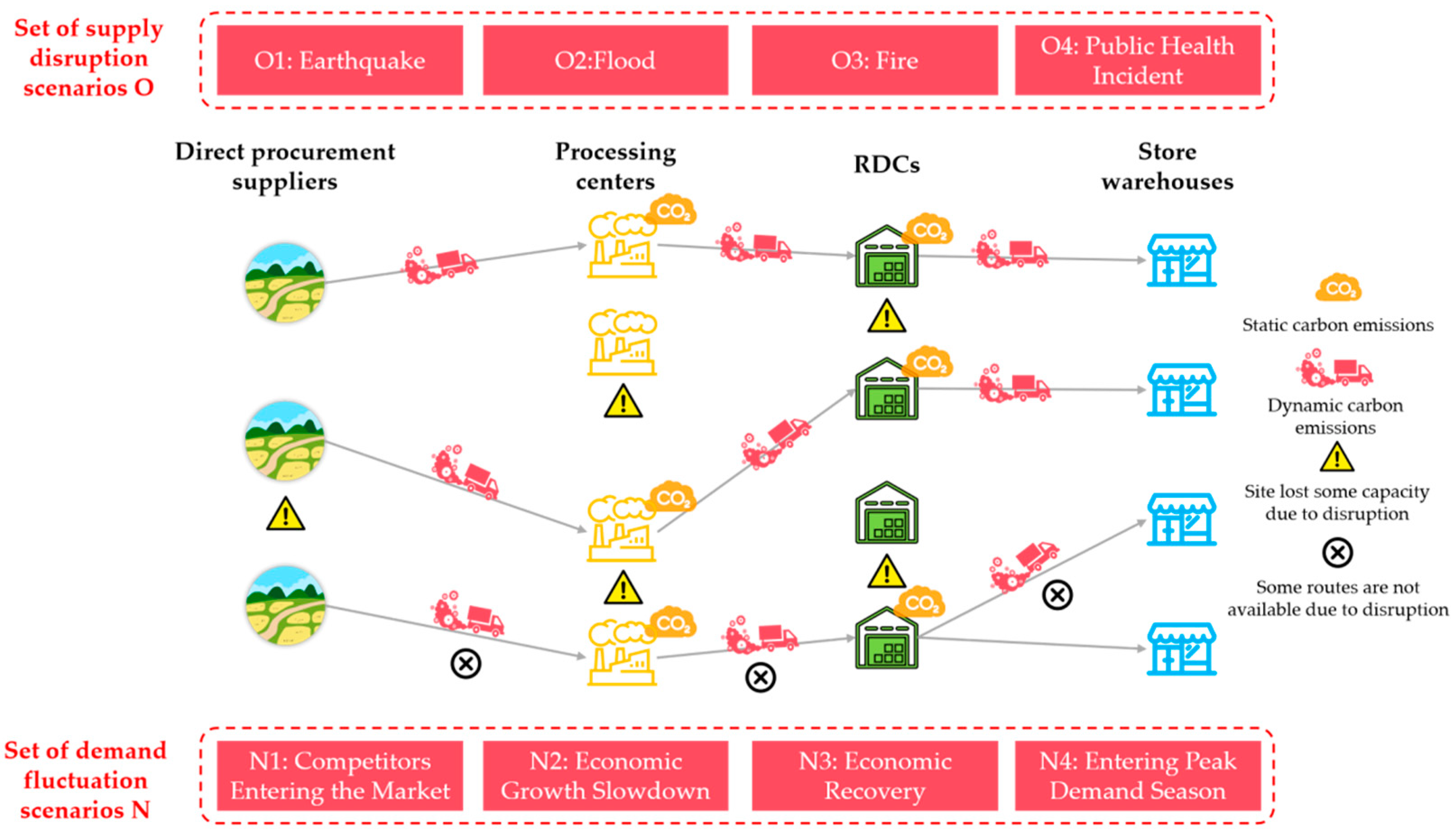
- This study innovatively designs and optimizes the RL-FPCN, considering the supply chain risks of supply disruptions and demand fluctuations simultaneously. The supply disruptions include the capacity loss of facility nodes and the unavailability of paths between facility layers. Meanwhile, this research adopts four resilience strategies for optimization, namely site strengthening, emergency inventory, cross-level procurement, and multi-route transportation, to effectively address the mentioned supply and demand risks.
- (C)
- This study provides a new idea for solving models. It innovatively integrates the improved OPTICS algorithm, considering temporal–spatial distance and the improved slime mold algorithm with a full iteration cycle, thus constructing the neighborhood search–swarm intelligence algorithm OTS-FICSMA [27]. The nodes with similar time and space dimensions are first clustered through this improvement to generate the initial solution. Then, the intervention optimization is carried out on the full cycle of the initial solution iteration to improve the quality of the solution continuously. Finally, the solution performance of the algorithm is greatly improved.
- (D)
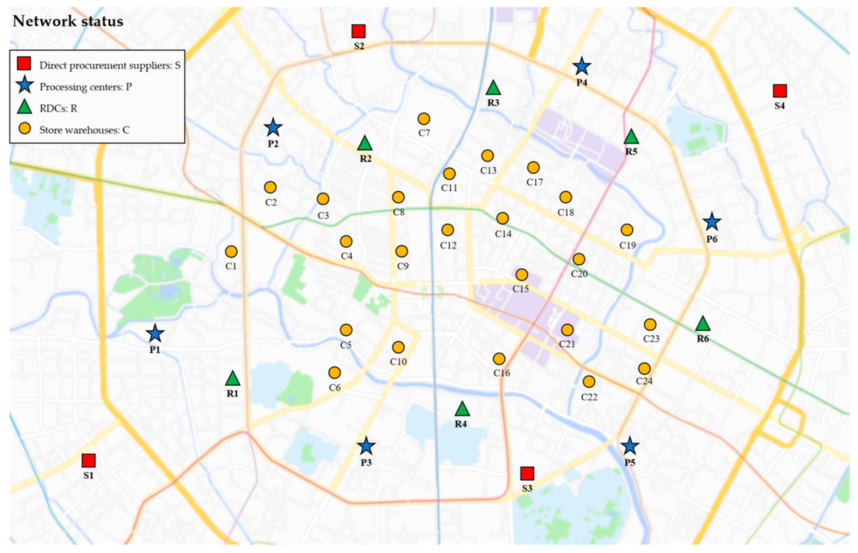
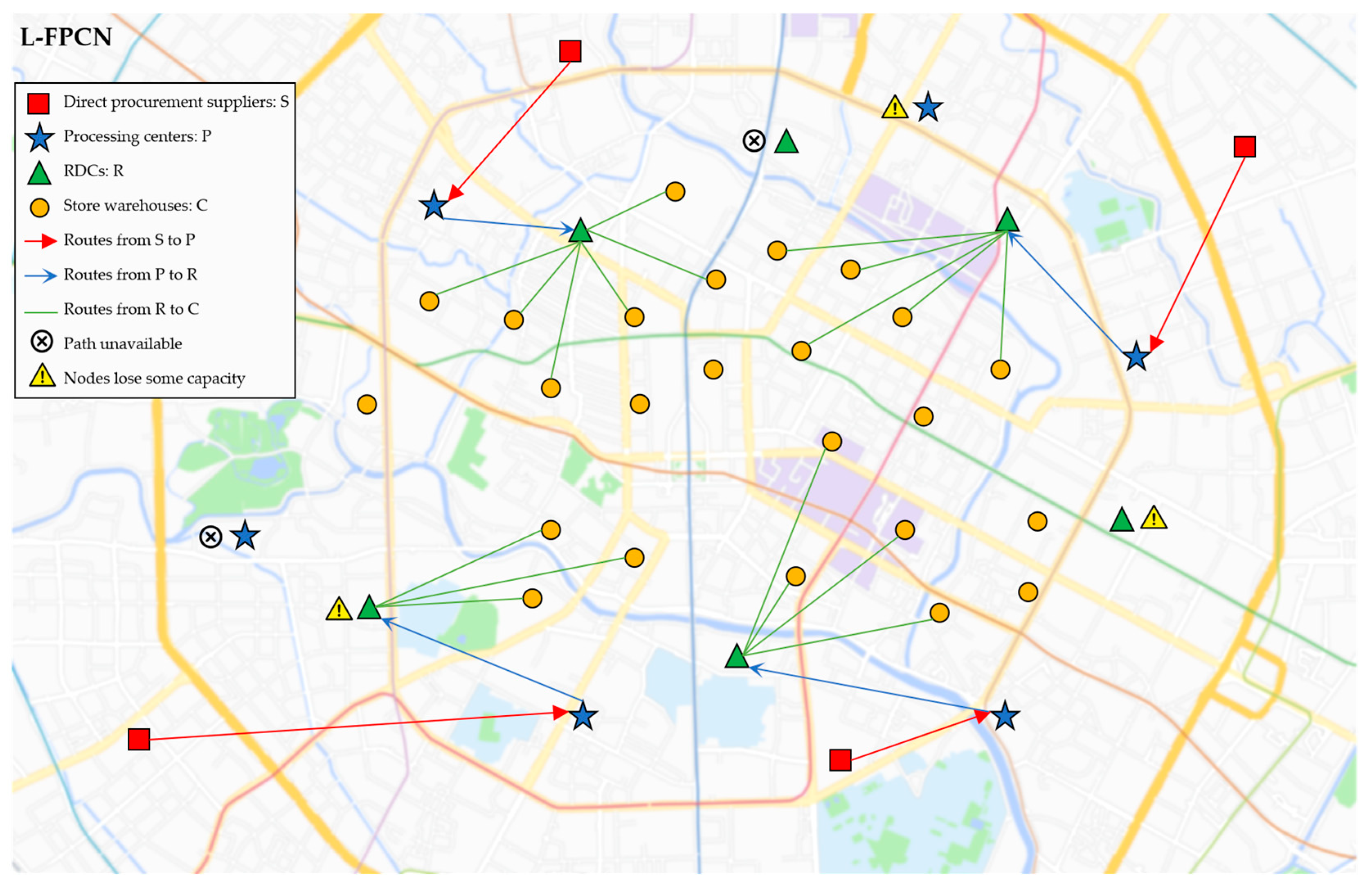
- At the practical application level, taking a real case in Chengdu, China as an example, the scenario analysis method is used to evaluate the impacts of the four resilience strategies and their collaborative performance in mitigating scenarios of supply disruptions and demand fluctuations. This work further compares the solution performance of the proposed OTS-FICSMA with those of algorithms with similar structures. The comparison verifies that the OTS-FICSMA effectively solves problems, providing strong support for the practical application of logistics distribution network optimization.
3. Problem Description and Model Construction
- I.
- Site strengthening strategy: this is reflected by investing more funds in processing centers and RDCs to reduce the proportion of capacity loss in disruption scenarios. In general, the level of strengthening is proportional to the operating costs and inversely proportional to capacity losses.
- II.
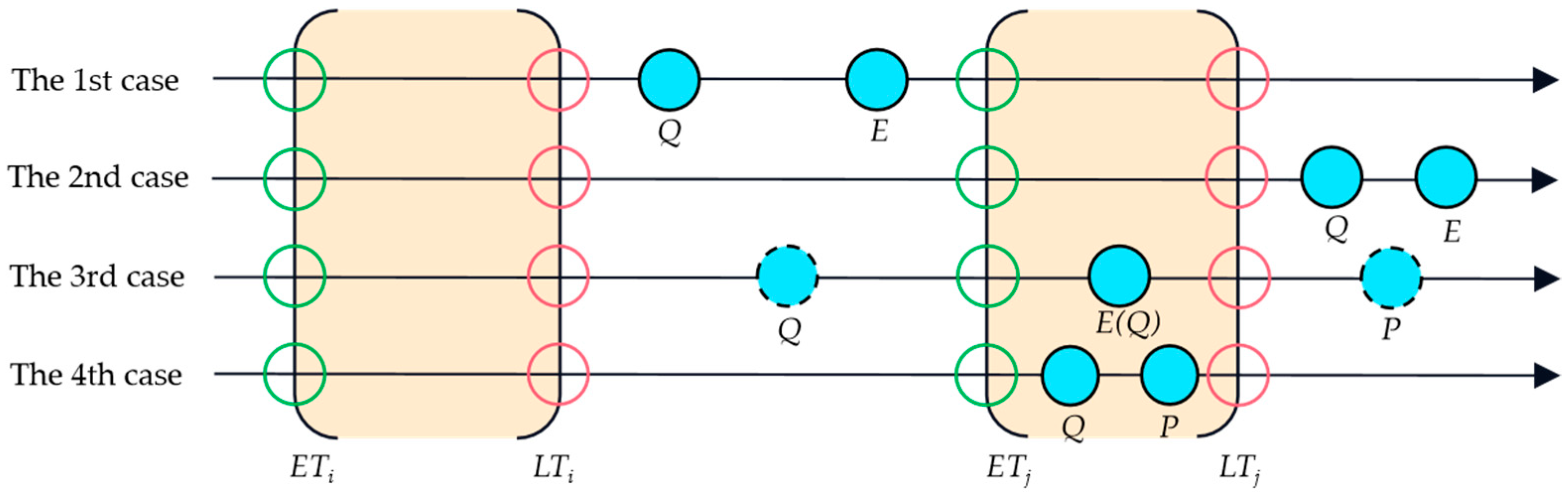
- Emergency inventory strategy: this means keeping additional emergency stock in processing centers and RDCs. In this case, when a node loses capacity, the emergency inventory will meet customer demand. Maintaining emergency inventory incurs emergency inventory costs.
- III.
- Cross-level procurement strategy: this allows fresh products to be directly transported from processing centers to store warehouses, saving the operation cost of RDCs and enhancing flexibility. However, the unit transportation cost of direct delivery to store warehouses is generally higher than through the RDCs.
- IV.
- Multi-route transportation strategy: this allows nodes at a certain level to receive raw materials or products from multiple sites at the previous level. Different route selections at various levels will incur the corresponding costs.
3.1. Model Assumptions
- When supply disruptions occur, a site’s inventory capacity or production capacity is lost, or certain routes between sites become unavailable.
- When demand fluctuations occur, the demand for a certain fresh product in the store warehouse will vary within a reasonable range.
- Supply disruptions and demand fluctuations are considered independent events.
- Carbon emissions are incorporated into the model as part of the operating costs.
- The carbon emission costs generated by on-site operations, production activities, and route transportation in FPCN are estimated by considering dynamic and static carbon emission tax rates.
- The emissions are related to the attributes of site operations and the quantity of production or transportation.
3.2. Symbols and Variables
3.3. Construction of the Basic Model
- (1)
- Objective Function
- (2)
- Constraints
- a.
- Route selection constraints: Equations (6)–(11) ensure that the transportation routes can only be selected among the open sites, that is, all the nodes covered by both ends of the transportation routes at all levels are the chosen sites.
- b.
- Site capacity constraints: Equations (12) and (13) state that the product flowing out of the accessible site cannot exceed its remaining capacity in the disruption and fluctuation scenarios. and represent the capacities of processing center j and RDC k for storing product p under the supply disruption scenario o, respectively.
- c.
- Traffic flow balance constraints: Equations (14)–(16) indicate that a product flow is generated between two nodes only if the path between them is selected and available. There are no capacity constraints on these routes. , , and are all binary variables, representing the road conditions from supplier i to factory j, from factory j to RDC k, and from RDC k to store warehouse l, respectively, under the supply disruption scenario o. If the road between the corresponding nodes is disrupted, the value is 1; otherwise, it is 0.
- d.
- Single route constraints: Equations (17)–(19) ensure a single transportation route between nodes at various levels.
- e.
- Goods flow balance constraints: Equations (20) and (21), respectively, indicate the flow balance constraints of the processing centers and RDCs. represents the conversion rate from raw material r to product p.
- f.
- Customer demand constraints: Equation (22) shows that the actual demand for the storehouse is composed of the quantity of received and unsatisfied goods. Equation (23) reflects the minimum service level constraint of the storehouse, which stipulates that the ratio of the amount of goods received to the actual demand shall not be lower than the minimum service standard.
- g.
- Equations (24) and (25) describe the binary variables, and Equation (26) ensures the positivity of the output results.
3.4. Robust Model Construction
- (1)
- Objective Function
- (2)
- Constraints
- a.
- Site strengthening constraints: Equations (34) and (35) indicate that at most one degree of strengthening can be chosen for the sites selected for strengthening.
- b.
- Emergency inventory constraints: Equations (36)–(39) indicate that emergency stock configuration is triggered only when a processing center or RDC is selected. In addition, the ratio between the emergency inventory capacity and the remaining capacity of the site is constrained by the maximum original capacity. and represent the capacities of processing center j and RDC k for storing product p, respectively.
- c.
- Cross-level procurement constraints: Equations (40)–(42) supplement the route selection from factories to RDCs and the freight flow information.
- d.
- Multi-route transportation constraints: Equation (43) supplements the traffic flow information from factories to RDCs. is a binary variable, representing the road conditions from factory j to store warehouse l under the supply disruption scenario o. If the road between the corresponding nodes is disrupted, the value is 1; otherwise, it is 0. In addition, , as a model adjustment factor, is a constant value of infinity.
4. Proposed OTS-FICSMA
4.1. Improved OPTICS Algorithm Considering Temporal–Spatial Distance (OTS)
4.2. Improved Slime Mold Algorithm with Full Iteration Cycle (FICSMA)
4.2.1. Basic Solving Principle of the Slime Mold Algorithm
4.2.2. Improvement Path of the Slime Mold Optimization Algorithm with Full Iteration Cycle
- (1)
- Multi-objective problem balancing mechanism
- (2)
- Pre-Stage Optimization Mechanism of Standard Brownian Motion
- (3)
- Post-stage Optimization Mechanism of the Ant Colony Optimization Algorithm
- (4)
- Instant Detection Mechanism of Iterative Variation
4.3. Analysis of the Algorithm Time Complexity
5. Case Simulation
5.1. Case Data Collection and Scenario Setting
5.1.1. Data Collection
5.1.2. Scenario Setting
5.2. Analysis of Supply Disruption Scenarios
- (1)
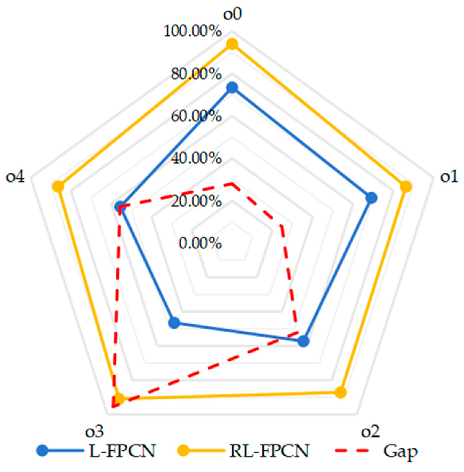
- Analysis of Service Level and Risk Resistance Ability
- (2)
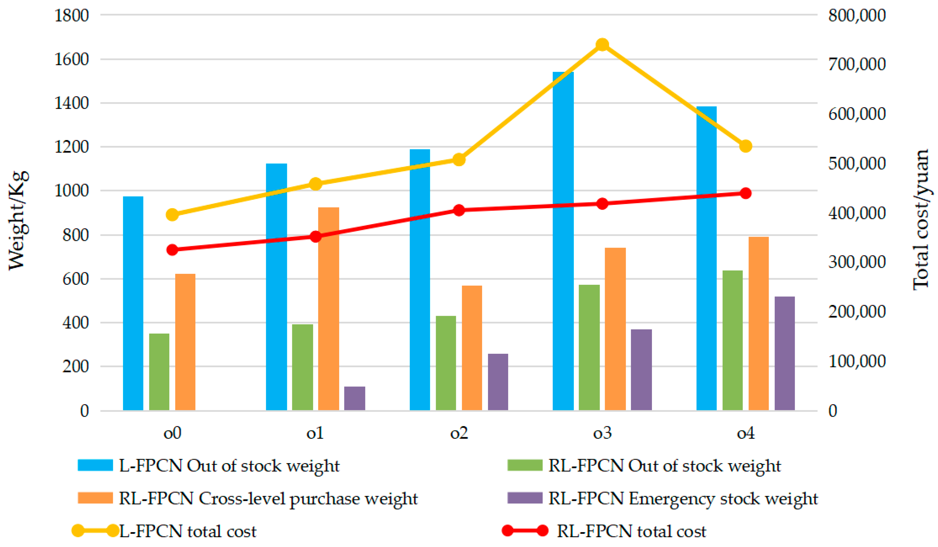
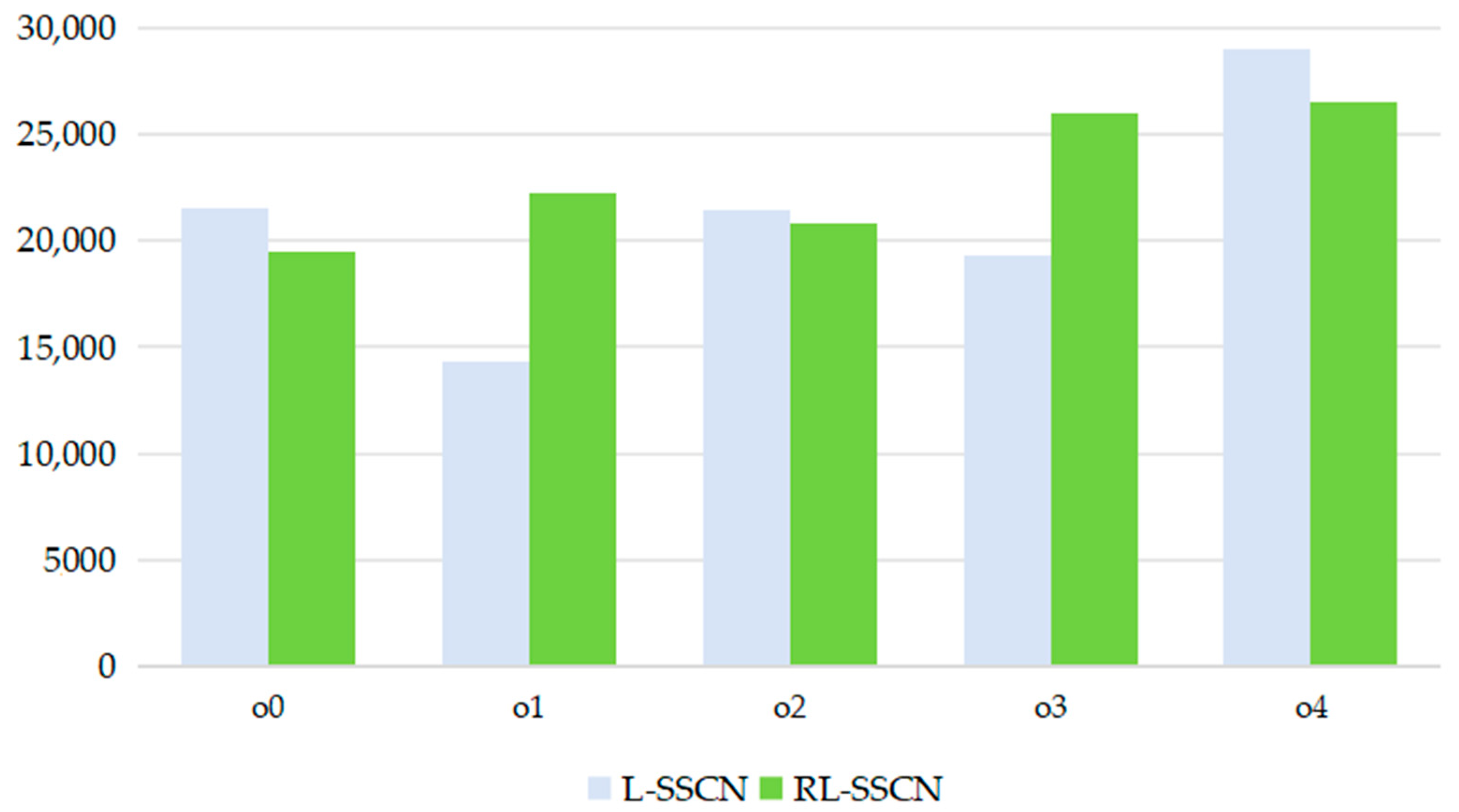
- Analysis of Operating Costs and Carbon Emissions
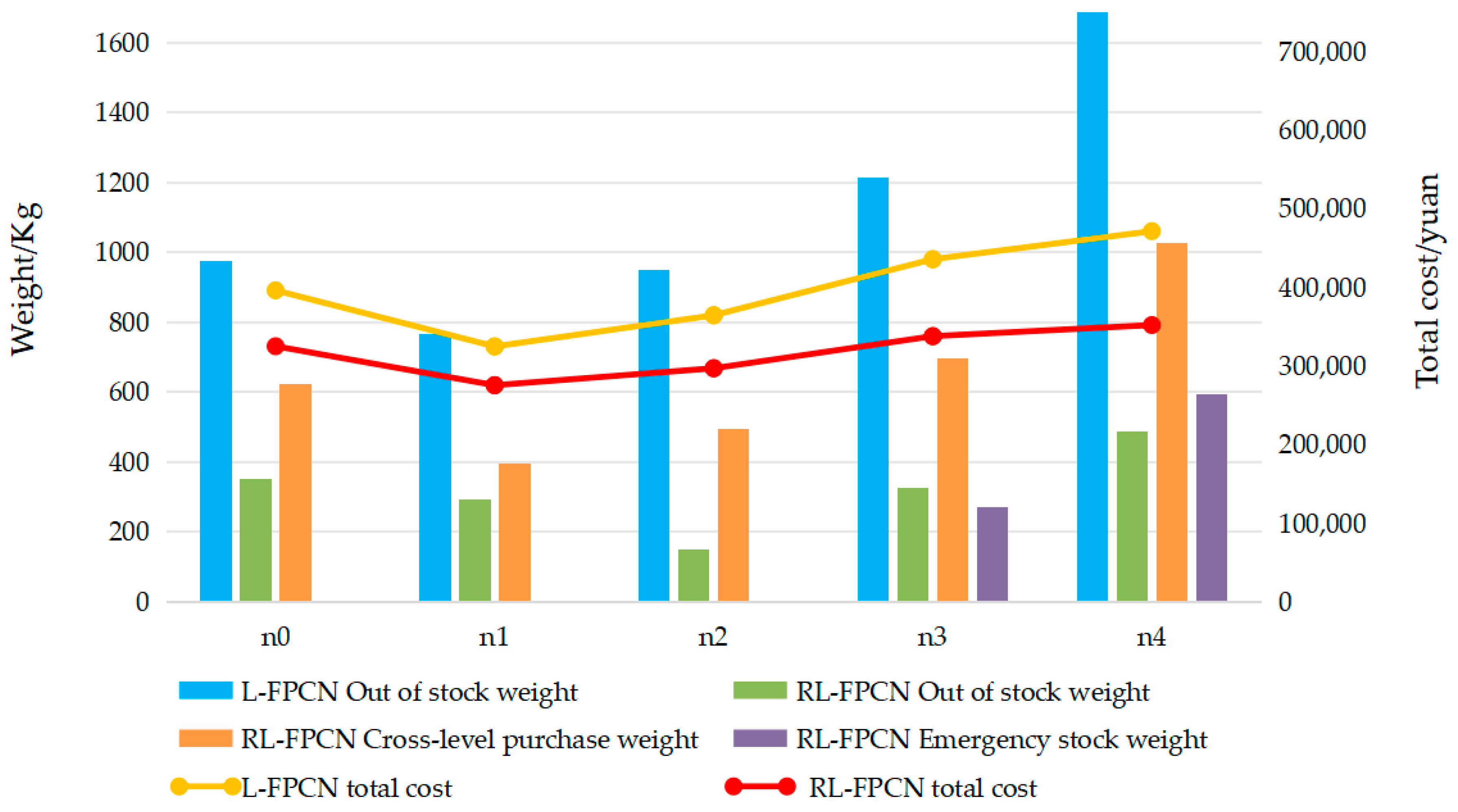
5.3. Analysis of Demand Fluctuation Scenarios
- (1)
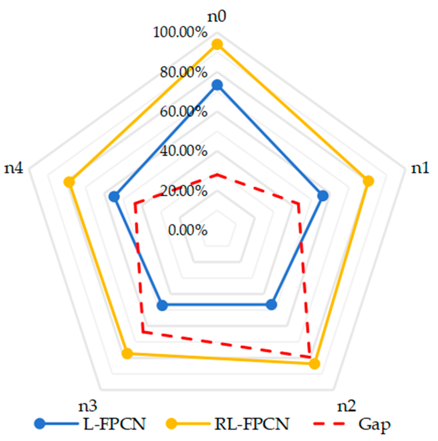
- Analysis of Service Level and Risk Resistance Ability
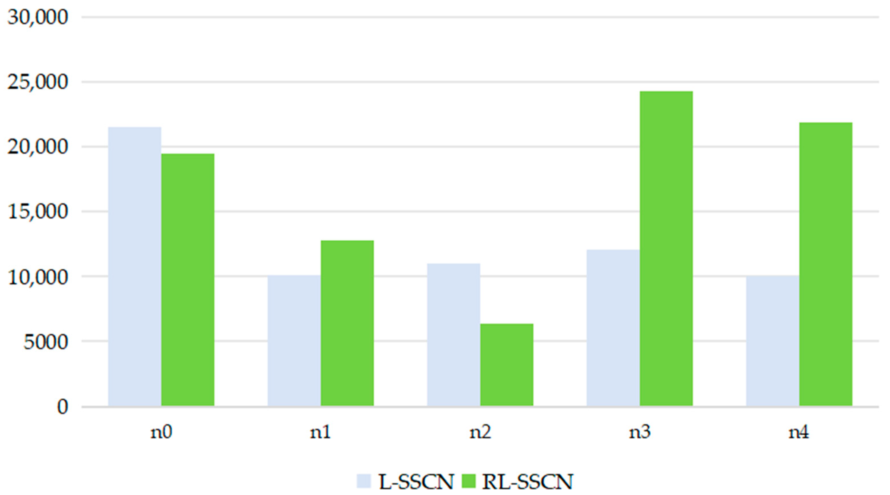
- (2)
- Analysis of Operating Costs and Carbon Emissions
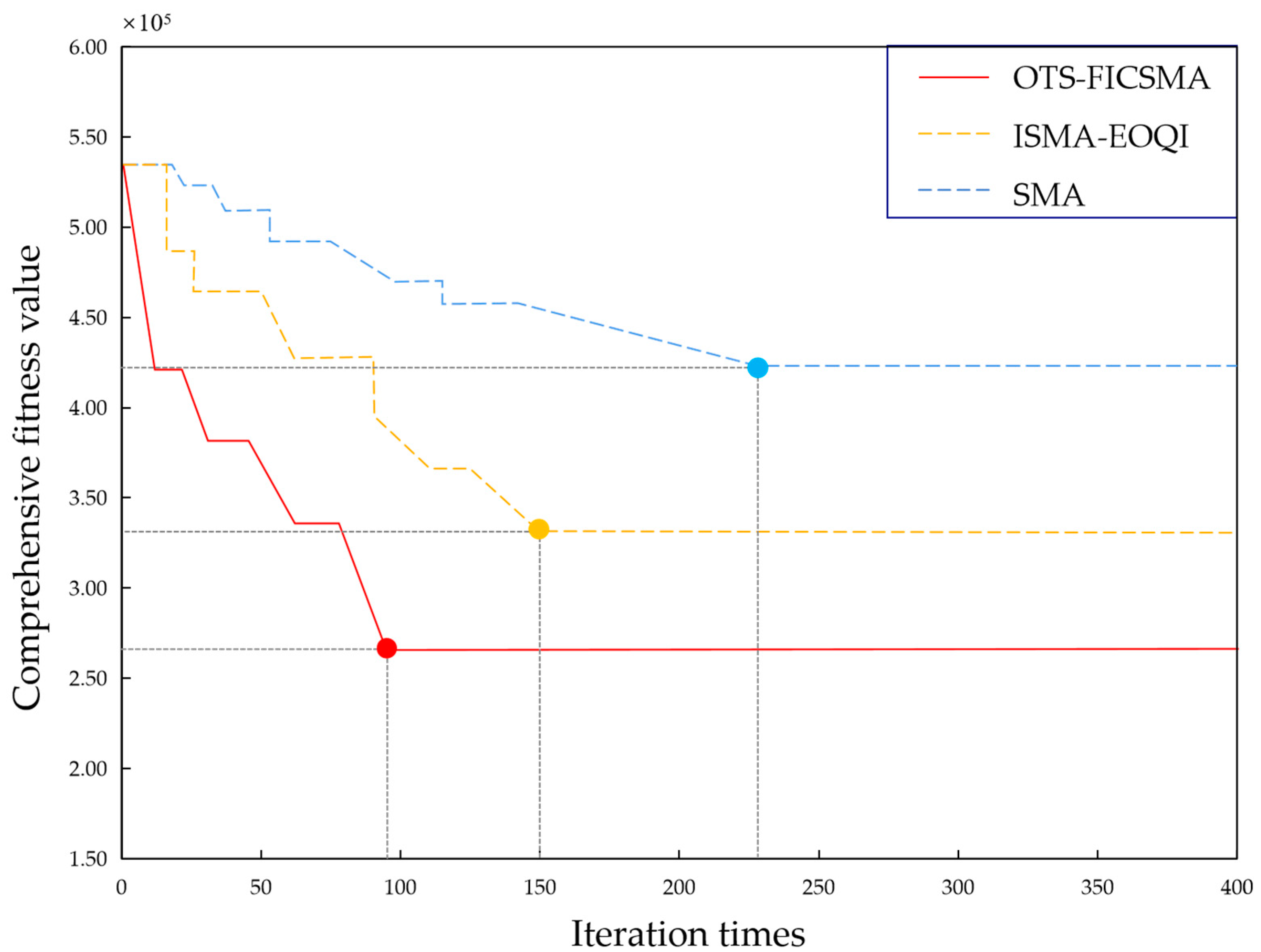
5.4. Comparison of Algorithm Performance
5.5. Sensitivity Analysis
6. Conclusions and Future Research
6.1. Conclusions
6.2. Management Insights
- (a)
- In terms of multi-objective optimization, the constructed RL-FPCN model aims to maximize the service level and minimize the operating cost, while also taking carbon emissions into account. This breaks through the limitations of traditional research that only focuses on economic and environmental objectives. Additionally, the study explores the balance relationship and collaborative optimization mechanism among multiple objectives, thus improving the application of multi-objective optimization theory in the cold chain field.
- (b)
- In terms of supply chain risk management, the four resilience strategies designed for supply disruptions and demand fluctuations clarify the response methods under different risk scenarios and their impact mechanisms on the supply chain, providing a more comprehensive perspective for the study of supply chain risk response strategies.
- (c)
- In terms of the design of hybrid heuristic algorithms, the OTS-FICSMA innovatively integrates neighborhood search and swarm intelligence algorithms, improving the solution efficiency and quality of the algorithm in complex scenarios, and providing a novel idea for algorithm design to solve complex optimization problems.
- (a)
- In the face of potential risks of supply disruptions and demand fluctuations, decision-makers can use the RL-FPCN model to make scientific location and routing decisions based on the risk probabilities. By flexibly applying the four resilience strategies, they can optimize the scheduling of facility resources, improve the service level, and reduce operating costs and carbon emissions.
- (b)
- When decision-makers are faced with conflicting objectives, they can use the ranking matrix proposed in this study to transform multi-objective numerical values with different dimensions into relative rankings, and conduct objective and intuitive comparisons within a unified framework, so as to achieve the balance of multiple objectives in the optimization scheme. In addition, when faced with the choice among different combinations of resilience strategies, they can rely on the solution results of the proposed algorithm, use it as a guide, and prioritize the selection of the best strategy under the current conditions.
- (c)
- In research modeling, relevant parameters and decision variables are categorized by facility location and routing, offering strong extensibility. SMEs’ decision-makers can adjust parameters as per businesses’ needs. This study provides clear references for key parameters to guide practical decision-making.
6.3. Limitations and Future Research
Author Contributions
Funding
Data Availability Statement
Conflicts of Interest
Appendix A
| Algorithm A1: OTS |
| 1 Inputs: the data set D, the neighborhood radius Eplison, the neighborhood threshold MinPts, the result queue O, the ordered queue Q 2 If (D == null) 3 Output the result queue O 4 Else 5 Take out the core point x and join the result queue O 6 Obtain neighbor object set N of x and join Q for ascending sort 7 While (Q == null) 8 Take out the top element q with the smallest rd in Q 9 Mark q as visited and join queue O 10 If q is not the core point 11 Re-execute the logic to determine whether Q is null 12 Else 13 Obtain neighbor object set N of q and join Q for ascending sort 14 While (O ≠ null) 15 Take out the top element p with the smallest rd in O 16 If (reachability distance of p > EpSilon) 17 If (core distance of p <= EpSilon) 18 Create cluster set C and add p to C 19 Else 20 Mark p as the noise point 21 Endif 22 Else 23 Add p to cluster C 24 Endif 25 Endwhile 26 Endif 27 Endwhile 28 Output the clustering results 29 Endif |
| Algorithm A2: FICSMA |
| 1 Inputs: clustering result set C, problem dimension D, population size N, maximum number of iterations tmax 2 Initialize position of slime mold Xi 3 Calculate the overall fitness for each slime mold and sort each fitness 4 Calculate the W by Equation (51) 5 Update the a by Equation (50) 6 t = 0 7 While t < tmax 8 If rand < z 9 Update Xi by Equation (52)-(1) 10 Detect iterative stalled detection by Equation (63) 11 Else 12 If t < tmax/2 13 Introduce a standard Brownian motion by Equation (56) 14 Detect iterative stalled detection by Equation (63) 15 Else 16 Introduce the ant colony search strategy by Equation (58) 17 Update the nodes and Tabek 18 If reach next destination node 19 Update pheromones τ by Equation (59) 20 Detect iterative stalled detection by Equation (63) 21 If d < D 22 t = tmax/2 # Re-compare by resetting loop state 23 Else 24 If n < N 25 rand = random() # Re-compare rand and z 26 Else 27 If t < tmax 28 Create cluster set C and add p to C 29 Else 30 Output optimization results 31 Endif 32 Endif 33 Endif 34 Else 35 t = tmax/2 # Re-compare by resetting loop state 36 Endif 37 Endif 38 Endif 39 t = t + 1 40 Endwhile |
Appendix B

| Facility Nodes | Fixed Operation Cost (CNY) | Capacity (kg) | Operation Carbon Emission Factor | Production Carbon Emission Factor | Unit Production Cost (CNY) | |
|---|---|---|---|---|---|---|
| Processing centers | P1 | 12,500 | 6125 | 0.13 | 0.36 | 50 |
| P2 | 17,000 | 6425 | 0.21 | 0.45 | 40 | |
| P3 | 22,500 | 6875 | 0.37 | 0.55 | 35 | |
| P4 | 28,000 | 7250 | 0.42 | 0.58 | 35 | |
| P5 | 25,500 | 7100 | 0.18 | 0.64 | 35 | |
| P6 | 14,000 | 6375 | 0.48 | 0.38 | 50 | |
| RDC | R1 | 17,500 | 2250 | 0.09 | —— | —— |
| R2 | 33,000 | 3050 | 0.16 | —— | —— | |
| R3 | 24,000 | 2500 | 0.23 | —— | —— | |
| R4 | 25,500 | 2650 | 0.28 | —— | —— | |
| R5 | 37,000 | 3200 | 0.12 | —— | —— | |
| R6 | 29,500 | 2850 | 0.26 | —— | —— | |
| Store Warehouse | Demand (kg) | Store Warehouse | Demand (kg) |
|---|---|---|---|
| C1 | 421 | C13 | 389 |
| C2 | 537 | C14 | 602 |
| C3 | 265 | C15 | 788 |
| C4 | 456 | C16 | 367 |
| C5 | 578 | C17 | 634 |
| C6 | 289 | C18 | 812 |
| C7 | 489 | C19 | 398 |
| C8 | 590 | C20 | 667 |
| C9 | 301 | C21 | 834 |
| C10 | 511 | C22 | 403 |
| C11 | 620 | C23 | 705 |
| C12 | 237 | C24 | 856 |
| Parameters | Values | Parameters | Values |
|---|---|---|---|
| ¥50 | 0.5 kgCO2e/(t·km) | ||
| ¥180 | 0.3 kgCO2e/(t·km) | ||
| ¥15 | 45 ¥/(tCO2e) | ||
| ¥20 | 0.65 | ||
| ¥25 | ¥500 | ||
| 0.6 kgCO2e/(t·km) | 150 km |
References
- China Cold Chain Logistics Development Report 2023. Available online: http://www.tjcn.org/tjnj/LLL/42826.html (accessed on 25 April 2025).
- BCI Supply Chain Resilience Report 2023. Available online: https://www.sgs.com/en/-/media/sgscorp/documents/corporate/white-papers/sgs-kn-supply-chain-resilience-report-2023-en.cdn.en.pdf (accessed on 25 April 2025).
- Jabbarzadeh, A.; Fahimnia, B.; Sabouhi, F. Resilient and sustainable supply chain design: Sustainability analysis under disruption risks. Int. J. Prod. Res. 2018, 56, 5945–5968. [Google Scholar] [CrossRef]
- Chowdhury, R.; Mim, S.J.; Tasnim, A.; Ng, K.T.W.; Richter, A. Supply-disposition storage of fresh fruits and vegetables and food loss in the Canadian supply chain. Ecol. Indic. 2025, 170, 113063. [Google Scholar] [CrossRef]
- Walmart Inc. 2023 Annual Report-Walmart Corporate. Available online: https://corporate.walmart.com/content/dam/corporate/documents/esgreport/reporting-data/tcfd/walmart-inc-2023-annual-report.pdf (accessed on 25 April 2025).
- Leng, L.; Wang, Z.; Zhao, Y.; Zuo, Q. Formulation and heuristic method for urban cold-chain logistics systems with path flexibility—The case of China. Expert Syst. Appl. 2024, 244, 122926. [Google Scholar] [CrossRef]
- Yadav, V.S.; Singh, A.R.; Gunasekaran, A.; Raut, R.D.; Narkhede, B.E. A systematic literature review of the agro-food supply chain: Challenges, network design, and performance measurement perspectives. Sustain. Prod. Consum. 2022, 29, 685–704. [Google Scholar] [CrossRef]
- Esteso, A.; Alemany, M.M.E.; Ortiz, Á. Impact of product perishability on agri-food supply chains design. Appl. Math. Model. 2021, 96, 20–38. [Google Scholar] [CrossRef]
- Hiassat, A.; Diabat, A.; Rahwan, I. A genetic algorithm approach for location-inventory-routing problem with perishable products. J. Manuf. Syst. 2017, 42, 93–103. [Google Scholar] [CrossRef]
- Paam, P.; Berretta, R.; García-Flores, R.; Paul, S.K. Multi-warehouse, multi-product inventory control model for agri-fresh products-A case study. Comput. Electron. Agric. 2022, 194, 106783. [Google Scholar] [CrossRef]
- Osvald, A.; Zadnik Stirn, L. A vehicle routing algorithm for the distribution of fresh vegetables and similar perishable food. J. Food Eng. 2008, 85, 285–295. [Google Scholar] [CrossRef]
- Pratap, S.; Jauhar, S.K.; Paul, S.K.; Zhou, F. Stochastic optimization approach for green routing and planning in perishable food production. J. Clean. Prod. 2022, 333, 130063. [Google Scholar] [CrossRef]
- Peng, Y.; Zhang, Y.; Yu, D.Z.; Luo, Y. Multiobjective Route Optimization for Multimodal Cold Chain Networks Considering Carbon Emissions and Food Waste. Mathematics 2024, 12, 3559. [Google Scholar] [CrossRef]
- Fathollahzadeh, K.; Saeedi, M.; Khalili-Fard, A.; Rabbani, M.; Aghsami, A. Multi-objective optimization for a green forward-reverse meat supply chain network design under uncertainty: Utilizing waste and by-products. Comput. Ind. Eng. 2024, 197, 110578. [Google Scholar] [CrossRef]
- Gholian-Jouybari, F.; Hajiaghaei-Keshteli, M.; Smith, N.R.; Rodríguez Calvo, E.Z.; Mejía-Argueta, C.; Mosallanezhad, B. An in-depth metaheuristic approach to design a sustainable closed-loop agri-food supply chain network. Appl. Soft Comput. 2024, 150, 111017. [Google Scholar] [CrossRef]
- Moghaddasi, B.; Ghafari Majid, A.S.; Mohammadnazari, Z.; Aghsami, A.; Rabbani, M. A green routing-location problem in a cold chain logistics network design within the Balanced Score Card pillars in fuzzy environment. J. Comb. Optim. 2023, 45, 129. [Google Scholar] [CrossRef]
- Christopher, M.; Peck, H. Building the resilient supply chain. Int. J. Logist. Manag. 2004, 15, 1–14. [Google Scholar] [CrossRef]
- Hasani, A.; Mokhtari, H.; Fattahi, M. A multi-objective optimization approach for green and resilient supply chain network design: A real-life case study. J. Clean. Prod. 2021, 278, 123199. [Google Scholar] [CrossRef]
- Jin, J.G.; Tang, L.C.; Sun, L.; Lee, D.H. Enhancing metro network resilience via localized integration with bus services. Transport. Res. Part E Logist. Transp. Rev. 2014, 63, 17–30. [Google Scholar] [CrossRef]
- Sabouhi, F.; Jabalameli, M.S.; Jabbarzadeh, A. An optimization approach for sustainable and resilient supply chain design with regional considerations. Comput. Ind. Eng. 2021, 159, 107510. [Google Scholar] [CrossRef]
- Alikhani, R.; Torabi, S.A.; Altay, N. Retail supply chain network design with concurrent resilience capabilities. Int. J. Prod. Econ. 2021, 234, 108042. [Google Scholar] [CrossRef]
- Benhamida, H.; Selim, H.M.; Benmamoun, Z.; Agarwal, V.; Jebbor, I.; Alabed, N. Fuzzy Multi-Criteria Decision-Making for Sustainable Risk Management. J. Posthumanism 2025, 5, 691–723. [Google Scholar] [CrossRef]
- Xie, F.; Chen, Z.; Zhang, Z. Research on Dynamic Takeout Delivery Vehicle Routing Problem under Time-Varying Subdivision Road Network. Mathematics 2024, 12, 962. [Google Scholar] [CrossRef]
- Foroozesh, N.; Karimi, B.; Mousavi, S.M. Green-resilient supply chain network design for perishable products considering route risk and horizontal collaboration under robust interval-valued type-2 fuzzy uncertainty: A case study in food industry. J. Environ. Manag. 2022, 307, 114470. [Google Scholar] [CrossRef]
- Mostaghim, N.; Gholamian, M.R.; Arabi, M. Designing a resilient-sustainable integrated broiler supply chain network using multiple sourcing and backup facility strategies dealing with uncertainties in a disruptive network: A real case of a chicken meat network. Comput. Chem. Eng. 2024, 188, 108772. [Google Scholar] [CrossRef]
- Shekarabi, H.; Vali-Siar, M.M.; Mozdgir, A. Food supply chain network design under uncertainty and pandemic disruption. Oper. Res. 2024, 24, 26. [Google Scholar] [CrossRef]
- Wang, H.; Ran, H.; Zhang, S. Location-routing optimization problem of country-township-village three-level green logistics network considering fuel-electric mixed fleets under carbon emission regulation. Comput. Ind. Eng. 2024, 194, 110343. [Google Scholar] [CrossRef]
- Zeng, L.; Liu, S.Q.; Kozan, E.; Burdett, R.; Masoud, M.; Chung, S.H. Designing a resilient and green coal supply chain network under facility disruption and demand volatility. Comput. Ind. Eng. 2023, 183, 109476. [Google Scholar] [CrossRef]
- Sun, M.; Xu, Y.; Xiao, F.; Ji, H.; Su, B.; Bu, F. Optimizing Multi-Echelon Delivery Routes for Perishable Goods with Time Constraints. Mathematics 2024, 12, 3845. [Google Scholar] [CrossRef]
- Cai, Z.; Gu, Z.; He, K. A self-adaptive density-based clustering algorithm for varying densities datasets with strong disturbance factor. Data Knowl. Eng. 2024, 153, 102345. [Google Scholar] [CrossRef]
- Alibaba Group Financial Annual Report 2024. Available online: https://static.alibabagroup.com/reports/fy2024/ar/ebook/CN/index.html (accessed on 22 February 2025).
- Chengdu Statistical Yearbook 2024. Available online: https://cdstats.chengdu.gov.cn/cdstjj/c178732/2024-12/31/content_025ae6eb8f4f4a27b6245a53b5f98b53.shtml (accessed on 22 February 2025).
- Semi-Annual Report of Yonghui Supermarket Co., LTD. 2024. Available online: https://www.yonghui.com.cn/upload/Inv/10407220.PDF (accessed on 22 February 2025).
- Guo, Y.X.; Liu, S.; Zhang, L.; Huang, Q. Elite inverse and quadratic interpolation for improved viscous bacteria algorithm. Comput. Appl. Res. 2021, 38, 3651–3656. [Google Scholar]
- Li, S.; Chen, H.; Wang, M.; Heidari, A.A.; Mirjalili, S. Slime mould algorithm: A new method for stochastic optimization. Futur. Gener. Comput. Syst. 2020, 111, 300–323. [Google Scholar] [CrossRef]
- Rashid, A.; Rasheed, R.; Ngah, A.H.; Amirah, N.A. Unleashing the power of cloud adoption and artificial intelligence in optimizing resilience and sustainable manufacturing supply chain in the USA. J. Manuf. Technol. Manag. 2024, 35, 1329–1353. [Google Scholar] [CrossRef]
- Zeng, L.; Hu, H.; Tang, H.; Zhang, X.; Zhang, D. Carbon emission price point-interval forecasting based on multivariate variational mode decomposition and attention—LSTM model. Appl. Soft Comput. 2024, 157, 111543. [Google Scholar] [CrossRef]


| Related Literature | Carbon Emission | Resilience Analysis | Customer Service Level | Solution Approach | Real-Case Analysis | |||
|---|---|---|---|---|---|---|---|---|
| Static | Dynamic | Disruption | Fluctuation | Strategies | ||||
| Leng et al. (2024) [6] | √ | √ | √ | SIA | ||||
| Paam et al. (2022) [10] | √ | √ | √ | BS | √ | |||
| Pratap et al. (2022) [12] | √ | √ | √ | SIA | ||||
| Peng et al. (2024) [13] | √ | √ | √ | SIA | √ | |||
| Fathollahzadeh et al. (2024) [14] | √ | √ | √ | SIA | √ | |||
| Gholian-Jouybari et al. (2024) [15] | √ | √ | √ | SIA | √ | |||
| Moghadda-si et al. (2023) [16] | √ | √ | √ | BS | ||||
| Hasani et al. (2021) [18] | √ | √ | √ | √ | NS | √ | ||
| Sabouhi et al. (2021) [20] | √ | √ | BS | √ | ||||
| Alikhani et al. (2021) [21] | √ | √ | √ | BS | √ | |||
| Benhamida et al. (2025) [22] | √ | √ | √ | BWM+ TOPSIS | √ | |||
| Xie et al. (2024) [23] | √ | √ | SIA | √ | ||||
| Foroozesh et al. (2022) [24] | √ | √ | √ | BS | √ | |||
| Mostaghim et al. (2024) [25] | √ | √ | √ | BS | √ | |||
| Shekarabi et al. (2024) [26] | √ | √ | BS | |||||
| This Study | √ | √ | √ | √ | √ | √ | NS-SIA | √ |
| Sets | ||
|---|---|---|
| Set of direct procurement suppliers, | ||
| Set of processing centers, | ||
| Set of RDCs, | ||
| Set of store warehouses, E | ||
| Set of raw materials produced by suppliers, | ||
| Set of fresh products, | ||
| Set of supply disruption scenarios, | ||
| Set of demand fluctuation scenarios, | ||
| Strengthening levels of sites under the site strengthening strategy, | ||
| Set of optional routes under the multi-route transportation strategy, | ||
| Parameters related to the low-carbon network | ||
| Route planning | Actual distance from direct procurement supplier i to processing center j | |
| Actual distance from processing center j to RDC k | ||
| Actual distance from RDC k to store warehouse l | ||
| Unit transportation cost of transporting raw material r from direct procurement supplier i to processing center j | ||
| Unit transportation cost of transporting product p from processing center j to RDC k | ||
| Unit transportation cost of transporting product p from RDC k to store warehouse l | ||
| Transportation carbon emission factor from direct procurement supplier i to processing center j | ||
| Transportation carbon emission factor from processing center j to RDC k | ||
| Transportation carbon emission factor from RDC k to store warehouse l | ||
| Location decision | Fixed operating cost of processing center j | |
| Fixed operating cost of RDC k | ||
| Ordering cost of product p | ||
| Quantity of product p ordered by RDC k each time | ||
| Inventory holding cost rate of RDC k | ||
| Operational carbon emission factor of processing center j | ||
| Operational carbon emission factor of RDC k | ||
| Production carbon emission factor of processing center j for producing product p | ||
| Unit cost of processing center j for producing product p | ||
| Others | Maximum service distance from RDC k to store warehouse l | |
| Penalty cost for the unmet demand of customer m for product p shipped from RDC l | ||
| Unit price of product p | ||
| Fixed carbon tax | ||
| Parameters related to theresilience network | ||
| Route planning | Actual distance from store warehouse l to processing center j under the cross-level procurement strategy | |
| Route selection cost from direct procurement supplier i to processing center j under the multi-route transportation strategy | ||
| Route selection cost from processing center j to RDC k under the multi-route transportation strategy | ||
| Route selection cost from processing center j to store warehouse l under the cross-level procurement and multi-route transportation strategies | ||
| Route selection cost from RDC k to store warehouse l under the multi-route transportation strategy | ||
| Unit transportation cost of transporting product p from processing center j to store warehouse l under the cross-level procurement strategy | ||
| Transportation carbon emission factor from processing center j to store warehouse l under the cross-level procurement strategy | ||
| Location decision | Fixed operating cost of processing center j after being strengthened with the strengthening level v | |
| Fixed operating cost of RDC k after being strengthened with the strengthening level v | ||
| Unit procurement cost of emergency inventory of product p purchased from processing center j | ||
| Unit procurement cost of emergency inventory of product p purchased from CDC k | ||
| Others | Probability of the occurrence of the supply disruption scenario o | |
| Probability of the occurrence of the demand fluctuation scenario n | ||
| Demand quantity of product p at store warehouse l under the supply disruption scenario o and demand fluctuation scenario n | ||
| Decision variables | ||
| Route planning | Binary variable = 1, if the service distance from RDC k to store warehouse l is less than or equal to [the maximum service distance]; and 0 otherwise | |
| Binary variable = 1, if the route w from direct procurement supplier i to processing center j is selected to operate; and 0 otherwise | ||
| Binary variable = 1, if the route w from processing center j to RDC k is selected to operate; and 0 otherwise | ||
| Binary variable = 1, if the route w from RDC k to store warehouse l is selected to operate; and 0 otherwise | ||
| Binary variable = 1, if the route w from processing center j to store warehouse l is selected; and 0 otherwise | ||
| Continuous variable: quantity of raw material r from direct procurement supplier i to processing center j under the supply disruption scenario o and demand fluctuation scenario n | ||
| Continuous variable: quantity of product p from processing center j to RDC k under the supply disruption scenario o and demand fluctuation scenario n | ||
| Continuous variable: quantity of product p from RDC k to store warehouse l under the supply disruption scenario o and demand fluctuation scenario n | ||
| Continuous variable: quantity of product p from processing center j to store warehouse l under the supply disruption scenario o and demand fluctuation scenario n | ||
| Location decision | Binary variable = 1, if processing center j strengthened with the strengthening level v is selected to operate; and zero otherwise | |
| Binary variable = 1, if RDC k strengthened with the strengthening level v is selected to operate; and zero otherwise | ||
| Continuous variable: quantity of product p in short supply at store warehouse l under the supply disruption scenario o and demand fluctuation scenario n | ||
| Continuous variable: quantity of emergency inventory of product p purchased from processing center j under the supply disruption scenario o and demand fluctuation scenario n | ||
| Continuous variable: quantity of emergency inventory of product p purchased from RDC k under the supply disruption scenario o and demand fluctuation scenario n | ||
| Objects | Optimization Scheme | |||||
|---|---|---|---|---|---|---|
| ··· | ||||||
| ··· | ||||||
| ··· | ||||||
| Scenario Classification | Influence | Probability | ||
|---|---|---|---|---|
| Supply Disruption Scenario Set O | o0 | Normal | The sites and routes are in a normal state. | 60% |
| o1 | Earthquake | The sites within the earthquake-affected area are disrupted; that is, they will lose 75% of their capacity. | 5% | |
| o2 | Flood | The routes between the affected sites are disrupted; that is, some paths will be unavailable for selection. | 15% | |
| o3 | Fire | The production capacity of the processing factory decreases by 75%. | 15% | |
| o4 | Public Health Incident | Some sites and the routes between sites are disrupted. | 5% | |
| Demand Fluctuation Scenario Set N | n0 | Normal | Customers meet the normal market demand. | 60% |
| n1 | Competitors Entering the Market | The demand decreases by 75%. | 10% | |
| n2 | Economic Growth Slowdown | The demand decreases by 25%. | 10% | |
| n3 | Economic Recovery | The demand increases by 25%. | 10% | |
| n4 | Entering the Peak Demand Season | The demand increases by 75%. | 10% | |
| Supply Disruption Scenario Set O | o0 | o1 | o2 | o3 | o4 | |
|---|---|---|---|---|---|---|
| Comparison of Service Levels | L-FPCN | 73.45% | 69.12% | 57.23% | 46.51% | 55.48% |
| RL-FPCN | 94.01% | 86.23% | 87.12% | 90.89% | 86.34% | |
| Gap | 27.99% | 24.75% | 52.23% | 95.42% | 55.62% |
| Supply Disruption Scenario O | Total Cost | Location Selection Cost | Inventory Cost | Path Selection Cost | Transportation Cost | Comprehensive Carbon Emission Cost | |
|---|---|---|---|---|---|---|---|
| o0 | L-FPCN | 396,244 | 182,946 | 144,788 | 0 | 46,955 | 21,555 |
| RL-FPCN | 325,172 | 196,339 | 45,524 | 9300 | 54,564 | 19,445 | |
| Gap | −17.94% | 7.32% | −68.56% | 0 | 16.20% | −9.79% | |
| o1 | L-FPCN | 458,430 | 208,906 | 154,858 | 0 | 80,363 | 14,303 |
| RL-FPCN | 351,966 | 201,290 | 52,689 | 9538 | 66,240 | 22,209 | |
| Gap | −23.22% | −3.65% | −65.98% | 0 | −17.57% | 55.28% | |
| o2 | L-FPCN | 507,644 | 268,798 | 175,442 | 0 | 41,982 | 21,422 |
| RL-FPCN | 405,267 | 272,705 | 67,193 | 10,699 | 33,880 | 20,790 | |
| Gap | −20.17% | 1.45% | −61.70% | 0 | −19.30% | −2.95% | |
| o3 | L-FPCN | 740,314 | 462,549 | 228,165 | 0 | 30,278 | 19,322 |
| RL-FPCN | 418,523 | 202,691 | 100,990 | 8872 | 79,980 | 25,990 | |
| Gap | −43.47% | −56.18% | −55.74% | 0 | 164.15% | 34.51% | |
| o4 | L-FPCN | 535,000 | 263,220 | 201,374 | 0 | 41,409 | 28,997 |
| RL-FPCN | 439,675 | 252,066 | 80,153 | 12,003 | 68,941 | 26,512 | |
| Gap | −17.82% | −4.24% | −60.20% | 0 | 66.49% | −8.57% |
| Demand Fluctuation Scenario N | n0 | n1 | n2 | n3 | n4 | |
|---|---|---|---|---|---|---|
| Service Level Comparison | L-FPCN | 73.45% | 56.12% | 46.61% | 47.18% | 54.76% |
| RL-FPCN | 94.01% | 80.30% | 83.67% | 77.24% | 78.61% | |
| Gap | 27.99% | 43.09% | 79.51% | 63.71% | 43.55% |
| Demand Fluctuation Scenario N | Total Cost | Location Selection Cost | Inventory Cost | Path Selection Cost | Transportation Cost | Comprehensive Carbon Emission Cost | |
|---|---|---|---|---|---|---|---|
| n0 | L-FPCN | 396,244 | 182,946 | 144,788 | 0 | 46,955 | 21,555 |
| RL-FPCN | 325,172 | 196,339 | 45,524 | 9300 | 54,564 | 19,445 | |
| Gap | −17.94% | 7.32% | −68.56% | 0 | 16.20% | −9.79% | |
| n1 | L-FPCN | 324,919 | 143,582 | 112,162 | 0 | 59,038 | 10,137 |
| RL-FPCN | 275,568 | 162,200 | 41,335 | 8928 | 50,291 | 12,814 | |
| Gap | −15.19% | 12.97% | −63.15% | 0 | −14.82% | 26.41% | |
| n2 | L-FPCN | 364,544 | 142,027 | 141,261 | 0 | 70,211 | 11,045 |
| RL-FPCN | 297,159 | 188,192 | 31,023 | 8885 | 62,641 | 6418 | |
| Gap | −18.48% | 32.50% | −78.04% | 0 | −10.78% | −41.89% | |
| n3 | L-FPCN | 435,869 | 196,359 | 139,522 | 0 | 87,915 | 12,073 |
| RL-FPCN | 337,959 | 153,670 | 68,403 | 13,586 | 77,967 | 24,333 | |
| Gap | −22.46% | −21.74% | −50.97% | 0 | −11.32% | 101.55% | |
| n4 | L-FPCN | 471,530 | 240,716 | 116,327 | 0 | 104,444 | 10,043 |
| RL-FPCN | 352,095 | 175,414 | 87,602 | 11,548 | 55,666 | 21,865 | |
| Gap | −25.33% | −27.13% | −24.69% | 0 | −46.70% | 117.71% |
| Algorithm | Parameter Settings |
|---|---|
| OTS-FICSMA | = 0.003, = 0.002, = 45, = 0.35, = 0.85, = 4, = 3, = 1.5 |
| ISMA-EOQI | = 0.003, ∈ [0.15, 0.30], ∈ [0.5, 0.7] |
| SMA | = 0.003 |
| Indicator | OTS-FICSMA | ISMA-EOQI | SMA |
|---|---|---|---|
| RLZ1 | 84.86% | 71.23% | 66.51% |
| RLZ2 | 359,776 | 424,857 | 511,469 |
| Site Strengthening Strategy | P4 | RDC: R6 | RDC: R1, R6 |
| Emergency Inventory Strategy | P5 RDC: R2 | P2, P3, P6 | P4, P5 RDC: R2 |
| Cross-Level Procurement Strategy | P3 → C5, C6, C10 P5 → C22, C23, C24 P6 → C19, C20 | P2 → C2, C3 P3 → C5, C6 P6 → C19, C20 | P4 → C13, C17, C18 |
| Multi-Route Transportation Strategy | P4 + P6 → R5 | P3 + P5 → R4 | S1 + S3 → P3 P3 + P5 → R4 |
| Effective Number of Iterations | 94 | 149 | 233 |
| Indicator | |||||||||
|---|---|---|---|---|---|---|---|---|---|
| BKS | Cmin | GAP | Cmin | GAP | Cmin | GAP | Cmin | GAP | |
| RLZ1 | 84.86% | 90.57% | 6.73% | 87.08% | 2.62% | 80.21% | −5.48% | 78.21% | −7.84% |
| RLZ2 | 359,776 | 319,523 | −11.19% | 335,269 | −6.81% | 375,416 | 4.35% | 389,692 | 8.32% |
| Site Strengthening Strategy | P4 | P2, R5 | P5 | R1 | R5 | ||||
| Emergency Inventory Strategy | P5, R2 | P5, R1 | R1, R5 | P5, R2 | P5 | ||||
| Cross-Level Procurement Strategy | P3 → C5, C6, C10 P5 → C22, C23, C24 P6 → C19, C20 | P2 → C1, C2, C3 P5 → C22, C23, C24 P6 → C19, C20 | P2 → C1, C2, C3 P3 → C5, C6, C10 P5 → C22, C23, C24 | P3 → C5, C6, C10 | P5 → C22, C23, C24 | ||||
| Multi-Route Transportation Strategy | P4 + P6 → R5 | P3 + P5 → R4 P4 + P6 → R5 | S1 + S2 → P3 P4 + P6 → R5 | P3 + P5 → R4 | S1 + S2 → P3 | ||||
| Indicator | |||||||||
|---|---|---|---|---|---|---|---|---|---|
| BKS | Cmin | GAP | Cmin | GAP | Cmin | GAP | Cmin | GAP | |
| RLZ1 | 84.86% | 94.23% | 11.04% | 90.96% | 7.19% | 77.35% | −8.85% | 75.47% | −11.07% |
| RLZ2 | 359,776 | 300,194 | −16.56% | 323,742 | −10.02% | 382,572 | 6.34% | 396,827 | 10.30% |
| Site Strengthening Strategy | P4 | R5 | R4 | P2, R5 | P4, R1, R6 | ||||
| Emergency Inventory Strategy | P5, R2 | R2 | P5 | P5, R1 | P2, R4 | ||||
| Cross-Level Procurement Strategy | P3 → C5, C6, C10 P5 → C22, C23, C24 P6 → C19, C20 | P5 → C22, C23, C24 | P3 → C5, C6, C10 P6 → C18, C19, C20 | P2 → C1, C2, C3 P5 → C22, C23, C24 | P2 → C1, C2, C3 P3 → C5, C6, C10 P4 → C13, C17, C18 | ||||
| Multi-Route Transportation Strategy | P4 + P6 → R5 | P3 + P5 → R4 | P4 + P6 → R5 | P3 + P5 → R4 P4 + P6 → R5 | S1 + S2 → P3 P4 + P6 → R5 | ||||
Disclaimer/Publisher’s Note: The statements, opinions and data contained in all publications are solely those of the individual author(s) and contributor(s) and not of MDPI and/or the editor(s). MDPI and/or the editor(s) disclaim responsibility for any injury to people or property resulting from any ideas, methods, instructions or products referred to in the content. |
© 2025 by the authors. Licensee MDPI, Basel, Switzerland. This article is an open access article distributed under the terms and conditions of the Creative Commons Attribution (CC BY) license (https://creativecommons.org/licenses/by/4.0/).
Share and Cite
Ran, H.; He, D.; Tang, H. Network Optimization of Fresh Products Cold Chain Considering Supply Disruption and Demand Fluctuation Under the Dual-Carbon Policy. Mathematics 2025, 13, 1539. https://doi.org/10.3390/math13091539
Ran H, He D, Tang H. Network Optimization of Fresh Products Cold Chain Considering Supply Disruption and Demand Fluctuation Under the Dual-Carbon Policy. Mathematics. 2025; 13(9):1539. https://doi.org/10.3390/math13091539
Chicago/Turabian StyleRan, Haojie, Dichen He, and Huajun Tang. 2025. "Network Optimization of Fresh Products Cold Chain Considering Supply Disruption and Demand Fluctuation Under the Dual-Carbon Policy" Mathematics 13, no. 9: 1539. https://doi.org/10.3390/math13091539
APA StyleRan, H., He, D., & Tang, H. (2025). Network Optimization of Fresh Products Cold Chain Considering Supply Disruption and Demand Fluctuation Under the Dual-Carbon Policy. Mathematics, 13(9), 1539. https://doi.org/10.3390/math13091539