Abstract
Accurate photovoltaic (PV) power generation forecasting is crucial for optimizing grid management and enhancing the reliability of sustainable energy systems. This study creates a novel hybrid model—MPA-VMD-BiGRU-MAM—designed to improve PV power forecasting accuracy through advanced decomposition and deep learning techniques. Initially, the Kendall correlation coefficient is applied to identify key influencing factors, ensuring robust feature selection for the model inputs. The Marine Predator Algorithm (MPA) optimizes the hyperparameters of Variational Mode Decomposition (VMD), effectively segmenting the PV power time series into informative sub-modes. These sub-modes are processed using a bidirectional gated recurrent unit (BiGRU) enhanced with a multi-head attention mechanism (MAM), enabling dynamic weight assignment and comprehensive feature extraction. Empirical evaluations on PV datasets from Alice Springs, Australia, and Belgium indicate that our hybrid model consistently surpasses baseline methods and achieves a 38.34% reduction in Mean Absolute Error (MAE), a 19.6% reduction in Root Mean Square Error (RMSE), a 4.41% improvement in goodness of fit, and a 33.91% increase in stability (STA) for the Australian dataset. For the Belgian dataset, the model attains a 96.32% reduction in MAE, a 95.84% decrease in RMSE, an 11.92% enhancement in goodness of fit, and an STA of 92.08%. We demonstrate the model’s effectiveness in capturing seasonal trends and addressing the inherent variability in PV power generation, offering a reliable solution to the challenges of instability, intermittency, and unpredictability in renewable energy sources.
Keywords:
photovoltaic power forecasting; hybrid deep learning model; marine predator algorithm (MPA); variational mode decomposition (VMD); multi-head attention mechanism MSC:
62M10; 68T07; 62P30; 94A12
1. Introduction
Global socio-economic development has markedly increased the demand for electricity, while irregular climate patterns and global instability have further strained conventional energy resources [1]. In response to these challenges, there is a growing emphasis on identifying and deploying sustainable energy solutions. Photovoltaic(PV) power generation has emerged as a highly promising alternative, leveraging solar energy through the charge separation phenomenon in PV cells to produce electrical power. This technology not only offers environmental benefits and renewable energy sources but also enhances energy safety.
As advancements in PV technology continue to evolve, the adoption and implementation of PV systems have surged globally. This trend is illustrated in Figure 1, which shows the long-term average potential power generation for a 1 kW peak grid-connected solar PV power plant, with the intensity of the red coloration indicating higher power generation capacities. Regions with deeper red hues are highlighted as having significant potential for PV power generation, underscoring the growing feasibility and importance of integrating PV systems into our energy infrastructure. Despite these advancements, effective prediction of PV power generation remains crucial for optimizing grid management and ensuring the stability and efficiency of renewable energy systems.
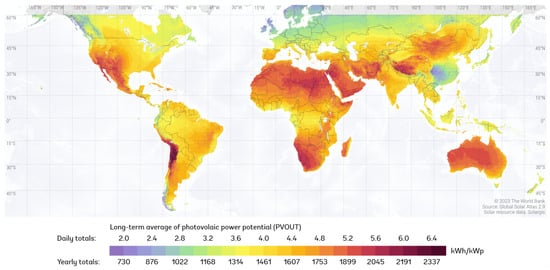
Figure 1.
Global PV power generation in 2023.
The rapid advancement in photovoltaic (PV) power prediction methodologies reflects the growing need for accurate and reliable forecasting in the face of increasing global energy demands and climate variability. PV power prediction techniques are generally categorized into physics-based models, statistical methods, machine learning approaches, and advanced artificial intelligence algorithms. Traditional methods such as support vector machines (SVMs) have been employed to predict PV output under varying weather conditions, demonstrating robust performance in handling different climatic scenarios [2,3]. However, recent studies have shown that machine learning techniques, particularly those integrating advanced decomposition and optimization algorithms, can enhance predictive accuracy. For instance, Zazoum (2022) compared SVM with Gaussian Processes Regression (GPR) for PV power prediction, revealing that the Matern 5/2 GPR model outperforms SVM in terms of accuracy by incorporating diverse meteorological parameters [4]. Similarly, Behera and Nayak (2020) proposed a hybrid model combining Empirical Modal Decomposition (EMD) with Extreme Learning Machine (ELM) to address the challenges of periodicity and fluctuations in PV data, achieving significant improvements in short-term forecasting [5]. Liu et al. (2021) further advanced this approach by integrating Ensemble Empirical Modal Decomposition (EEMD) with ELM, demonstrating enhanced convergence and stability across various weather conditions [6].
The field of photovoltaic power generation forecasting has also shown technological innovation in different aspects. Guo et al. (2024) adopted a deep fusion technology and a multi-task joint learning framework to effectively integrate heterogeneous data sources and capture long-term dependencies, enhancing the model’s ability to detect photovoltaic power change patterns [7]. Miraftabzadeh and Longo (2023) introduced a new prediction model based on deep learning technology and optimized by a Bayesian optimization algorithm, which can predict the high-resolution time step of the previous day’s photovoltaic power generation [8]. Tang et al. (2025) proposed a short-term PV hybrid prediction model, combined with meteorological data to extract key features, built a prediction model based on the iTransforme network, and introduced the attention mechanism [9], and Xu (2025) integrated a hybrid integration model (RLHE) based on stochastic learning and integrated three stochastic learning algorithms to construct the prediction interval of probabilistic PV prediction [10]. Liu et al. (2025) designed IFFT former, a hybrid deep learning model. DIF and LOF were used to construct a data preprocessing module, and the time series was decomposed into seasonal and trend components and modeled separately. MLP is used to fit the predicted trend component with the seasonal component predicted by the ProSparse self-attention mechanism based on information interaction, so as to realize the medium- and long-term PV power prediction [11]. Zhao (2024) proposed a digital twin (DT) model based on the domain matching Transformer, which uses CNN for domain invariant feature extraction, a Transformer for photovoltaic performance prediction, and DANN for domain self-adaptation [12]. Wang et al. (2024) proposed a new model of gradient-lifting dendritic (GBDD) networks. It uses greedy function approximation to grasp the correlation between forecast residual and meteorological factors during sub-model training and to reduce prediction error [13]. Yang et al. (2025) proposed a new multi-site hourly photovoltaic power prediction algorithm and the DEST-GNN graph network, which represented the correlation of photovoltaic power stations through undirected graphs, filtered the weak correlations by sparse spatio-temporal attention, and proposed an adaptive GCN to capture the implicit spatio-temporal dependence [14]. Chen et al. (2024) proposed a new short-term forecast method for photovoltaic power generation. Firstly, fuzzy C-means clustering (FCM) is used to classify the PV sample set and reduce the data variability. Subsequently, the PV physical mechanism model is integrated into the first layer of the integrated learning framework and is combined with LSTM and LGBM for the prediction.The mechanism model constrains the power generation boundary through physical laws and inhibits the prediction bias of the data-driven model [15]. Zhu et al. (2024) constructed a combination model of ultra-short-term photovoltaic power generation prediction based on the attention mechanism, selected key climate variables through Pearson analysis, classified weather by SCF, established a CNN prediction model, and added an ECA module to improve accuracy [16].
The application of Variational Mode Decomposition (VMD) has gained traction in recent studies, with Netsanet et al. (2022) integrating VMD with Ant Colony Optimization (ACO) and Recurrent Neural Networks (RNNs) to achieve 97.68% of the total variation in PV power prediction [17]. Similarly, Sun and Zhao (2020) utilized VMD combined with Convolutional Long Short-Term Memory (ConvLSTM) networks for wind power forecasting, showcasing its potential in improving operational performance [18]. More complex hybrid models, such as those incorporating Smooth Wavelet Transform (SWT), LSTM, and Deep Neural Networks (DNNs), have also been explored, as demonstrated by Ospina et al. (2019) [19].
Recent advancements in neural network architectures, including Bidirectional Long Short-Term Memory (BiLSTM) networks with attention mechanisms, have further improved forecasting accuracy and robustness. Zhou et al. (2019) proposed a BiLSTM model with an attention mechanism, achieving high performance across different seasons and prediction ranges [20]. Moreover, Ju et al. (2020) developed a two-step neural network that integrates Bidirectional LSTM with an Exponential Moving Average-preprocessed ANN, attaining high accuracy with various data types despite potential issues with missing data [21].
The latest approaches also include hybrid models utilizing the Whale Optimization Algorithm (WOA) and neural network frameworks. Yu et al. (2023) combined double-layer decomposition with WOA and BiLSTM–Attention to significantly reduce forecasting errors and enhance model reliability [22]. Despite these advancements, computational complexity and model optimization remain critical challenges, necessitating further research to balance accuracy and efficiency.
Traditional methods often struggle with capturing intricate temporal patterns and seasonal variations, while single artificial models, though promising, face issues related to computational efficiency and overfitting. In this paper, we have proposed a novel hybrid model that leverages the Marine Predator Algorithm (MPA) for optimized hyperparameter tuning, Variational Mode Decomposition (VMD) for effective data decomposition, and the Bidirectional Gated Recurrent Unit (BiGRU) combined with a multi-head attention mechanism (MAM) for enhanced predictive performance, which not only improves accuracy but also enhances the model’s adaptability and robustness for providing a significant advancement in smart PV power prediction and also effectively mitigates issues such as aliasing, over-enveloping, under-enveloping, and boundary effects. The integration of these methodologies addresses the inherent non-linearity and volatility of the solar power generation series, offering significant improvements with more predictive accuracy and real-time adaptability.
This paper is structured as follows: In Section 2, we have detailed the initial stage of our hybrid model, the MPA-VMD-BiGRU-MAM, which employs the Kendall correlation coefficient to identify significant correlations among influencing factors. This process ensures robust input selection for further processing, setting a solid foundation for accurate forecasting. The optimization of Variational Mode Decomposition (VMD) parameters using the Marine Predator Algorithm (MPA) is elaborated on, explaining how MPA enhances the decomposition of photovoltaic (PV) power time series into informative sub-modes, providing a nuanced analysis of the data preprocessing that is critical for the subsequent layers of our model. Then, the integration of the optimized sub-modes into a bidirectional gated recurrent unit (BiGRU) is implemented, which is further enhanced with a multi-head attention mechanism (MAM). In Section 3, we conduct empirical evaluations of our model through comprehensive datasets from Alice Springs, Australia, and Belgium. We compare MPA-VMD-BiGRU-MAM’s performance against several benchmark models, including variants of GRU and BiGRU, demonstrating significant improvements in forecasting accuracy. A detailed statistical analysis is provided to quantify the enhancements in Mean Absolute Error (MAE), Root Mean Square Error (RMSE), goodness of fit, and stability (STA), illustrating the substantial gains achieved by our model. This section also explores how the enhanced predictive capability of the MPA-VMD-BiGRU-MAM model addresses the challenges of instability, intermittence, and randomness in photovoltaic energy generation. The final section summarizes the research outcomes and discusses future research directions.
2. Methodology
2.1. Kendall Correlation Coefficient
Photovoltaic (PV) power production is subject to fluctuations driven by a range of climatological variables including solar irradiance, ambient temperature, humidity, and wind velocity. To quantitatively assess the interdependencies between these environmental factors and PV output, the Kendall correlation coefficient is employed. This non-parametric measure of correlation is particularly advantageous in scenarios where the data deviate from a normal distribution, unlike the Pearson correlation coefficient, which presupposes normality. The computation of the Kendall correlation coefficient is delineated in Equation (1).
where P and Q are the number of consistent and incompatible pairs, respectively. N is the total number of observed pairs. Both A and B are part of the total N. The variables A and B are consistent or harmonious if and ; otherwise, they are inconsistent or disharmonious [23]. Here, i and j indicate the rank of the ith and jth observations, = 1, 2, L, n.
2.2. Marine Predator Algorithm
The Marine Predator Algorithm (MPA) is an optimization methodology inspired by the foraging strategies and encounter rate policies observed between predators and prey within marine ecosystems [24]. This algorithm metaphorically adopts these natural interactions to enhance optimization processes. In this context, “prey” represents potential solutions, while “predators” embody the search strategy aimed at continually refining these solutions towards an optimal state. The application of MPA in this research involves three distinct phases:
(a) Initiation Phase: The optimization process begins with the MPA algorithm by stochastically initializing the positions of the “prey” within the designated search space. The updating position is mathematically articulated in Equation (2), setting the foundation for iterative improvement based on the dynamics of predator–prey interactions.
where, represents the lower limit of the search space, and represents the upper limit of the search space.
(b) Optimal Stage: At this juncture in the MPA optimization process, when the “carnivore” (representative of the optimization algorithm) exhibits a superior speed relative to the “prey” (potential solutions), the algorithm’s behavior shifts towards an exploratory phase. This transition is mathematically formalized and articulated in Equation (3), where the exploration strategy is systematically outlined to enhance the search for the optimal solution.
where is the moving step size; is the Brownian walk random vector with a normal distribution; means an elite matrix constructed by top predators; is a prey matrix with the same dimensions as the elite matrix; ⊗ is a term-wise multiplication operator; R is random vector with uniform distribution; n is the population size; and p is set as equal to 0.5 [25].
During the intermediate stage of the MPA optimization cycle, when the velocities of the predator and prey converge, the dynamics of the model adapt. In this phase, the prey evolves following the Lévy flight strategy, renowned for its efficiency in exploring diverse and large-scale search spaces. Concurrently, the predator employs an exploratory tactic influenced by Brownian motion strategies. This approach facilitates a gradual transition from exploratory to exploitative behaviors, optimizing the search process for potential solutions. The mathematical framework governing these iterative steps is detailed in Equations (4) and (5), encapsulating the systematic progression towards optimal convergence.
where is the random vector with a Lévy distribution and CF is the adaptive parameter to control the predator’s moving step length.
When the velocity of the “carnivore”—representing the optimization algorithm—lags behind that of the “prey”, the algorithm adopts an evolutionary strategy modeled on Lévy flight [26]. This strategy is characterized by random walks with step lengths drawn from a Lévy distribution, known for facilitating efficient exploration of vast search spaces by enabling large jumps. This adaptive mechanism is mathematically encapsulated in Equation (6), delineating the strategic shift to maintain the efficacy of the search process.
(c) Dynamic Adaptation: Fish Aggregating Devices (FADs) or oceanic whirlpools significantly influence the foraging behaviors of marine predators. These natural phenomena are harnessed to facilitate the management of Marine Protected Areas (MPAs), providing a strategic advantage by mitigating premature convergence and evading transient local optima during the optimization process. This ensures a dynamic and robust exploration of the solution space, enhancing algorithmic efficacy. The iterative modifications incorporated through this approach are detailed in Equation (7).
where FADs (Fish Aggregating Devices) represent an influence probability set at a value of 0.2, signifying their moderate impact on the behavior of marine predators within the algorithm. The relationship among various components such as the binary vector U, the random number r, and indices r1 and r2 within the prey matrix, is structured as follows: r is defined as a random number uniformly distributed within the interval [0, 1], serving as a stochastic component that governs the interaction dynamics and variability in predator–prey interactions.
2.3. Variational Mode Decomposition
The Variational Mode Decomposition (VMD) method excels in adaptively decomposing non-stationary waveforms and sequences into their constituent components. Specifically, it dissects the original signal f into k modes, each characterized by a constrained bandwidth centered within the spectrum. This method strategically minimizes the sum of the estimated bandwidths for each mode, ensuring that the aggregate of all decomposed modes closely aligns with the original signal. This optimization criterion, crucial for maintaining signal integrity during decomposition, is formally defined in Equation (8).
where f is the original signal, is the mode vector, and is the frequency of modal center. * represents the analytic signal under the Hilbert transform, when the sum of the bandwidths of the center frequencies of each modal component is the smallest modal function and the center frequency , , is the analytic signal under the Hilbert transform. is the pulse signal and is the exponential correction item (the exponential correction is to solve the amplitude amplification problem of the decomposition results, thereby improving the stability and accuracy of decomposition). is conditioned by Gaussian smoothing (i.e., the square root of the L2 norm) to obtain a bandwidth description of each modal function and is the gradient of the two-norm, which is used here to prevent the model from over-predicting.
We borrow the Lagrangian function to convert the conditional variational query into an unconditional variational query [27]:
where is the penalty parameter and is a Lagrange multiplier.
The corresponding updating formula of modal component and center frequency is as given in Equations (10) and (11).
where is the frequency and , , and represent the Fourier transforms of , , and , respectively.
Building on the Variational Mode Decomposition (VMD) method’s ability to break down complex, non-stationary signals, we will next outline the specific steps involved in applying the VMD technique. We have detailed the process by which the VMD algorithm divides a signal into distinct modes, each with a carefully adjusted bandwidth to make our method clear and replicable, ensuring that the practical application of VMD aligns well with the theoretical concepts we have discussed.
Step 1. Initialize the basic parameters, such as mode number k, bandwidth limit, noise tolerance, frequency domain expression, center frequency, Lagrange multiplier, etc.
Step 2. Update the modal and center of gravity amplitude .
Step 3. Update according to the iteration .
Step 4. Given the discriminant accuracy , stop the iteration when
is satisfied, and then return to step (2) to finally obtain the decomposed mode and complete the modal decomposition.
In the application of the Marine Predator Algorithm (MPA) to optimize the Variational Mode Decomposition (VMD) parameters, the choice of the penalty factor and the number of decomposition layers k is critical to achieving high-quality signal decomposition. In this study, we employ the mean value of dispersion entropy as the fitness function for MPA, targeting the minimization of dispersion entropy to refine our objective function. This approach facilitates the precise determination of the optimal values for k and through iterative optimization. The process is structured into five distinct steps, visually represented and detailed in Figure 2.
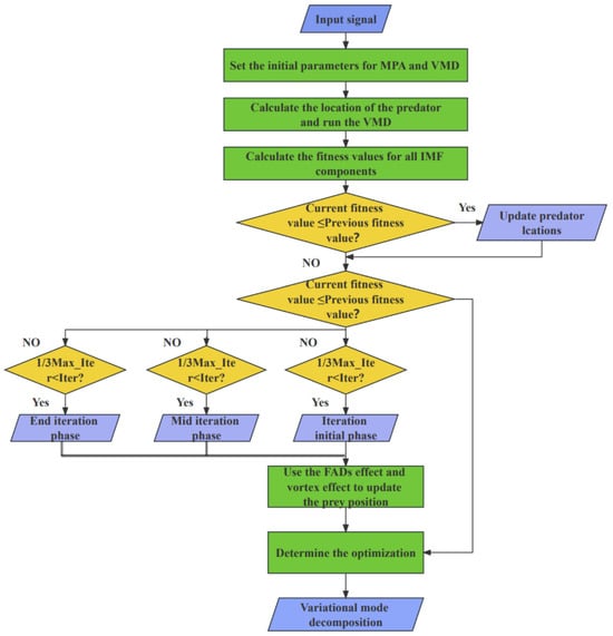
Figure 2.
The flow of the MPA-VMD algorithm.
2.4. Bidirectional Gated Recurrent Unit
While Long Short-Term Memory (LSTM) networks effectively mitigate the issue of vanishing gradients in extensive time series analysis, they are often computationally intensive. Gated Recurrent Units (GRUs) streamline the architecture of LSTMs, featuring a less complex model structure that not only reduces computational demands but also enhances convergence, as depicted in Figure 3. Despite these improvements, GRUs inherently process data unidirectionally, relying exclusively on past data for predictions.
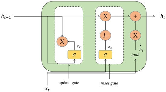
Figure 3.
Framework of GRU.
To address this limitation, the Bidirectional Gated Recurrent Unit (BiGRU) model employs a two-fold neural network strategy. One network processes data in a forward direction, capturing past contextual information, while the other processes data backwards, harnessing future contextual insights. This bidirectional mechanism enables the model to synthesize insights from both past and future data points, significantly refining the accuracy of the predictions and aligning them more closely with the actual values.
The architectural configuration of the Bidirectional Gated Recurrent Unit (BiGRU) network is illustrated in Figure 4, which delineates its four primary components: an input layer, a forward hidden layer, a backward hidden layer, and an output layer. The input layer serves as the initial receptacle for data, which are subsequently transmitted to both the forward and backward hidden layers. This dual-layer setup facilitates the bidirectional flow of data, enabling the network to process information from both past and future contexts simultaneously. The outputs generated by the network are a synthesis of the computations performed by both the forward and backward GRU networks, resulting in a sequence prediction that is integrative and comprehensive [28].
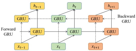
Figure 4.
Framework of BiGRU.
The calculation process is shown in Equations (12)–(15), where x is the input vector at time point t.
and are the updating and resetting gate, respectively, is the hiding layer for candidate selection, is the state of the hiding layer at time point , W and U are weights, b is the intercept, and is the sigmoid function. The network structure of BiGRU is described in Equations (16)–(18).
where and are the state of the forward and backward hidden layers at time t, and are the corresponding weights, and is the intercept of the hiding layer at time t [29].
2.5. Multi-Head Attention Mechanism
The attention mechanism (AM) is inspired by human perceptual and cognitive faculties. It is designed to enable neural networks to dynamically prioritize specific segments of the input while processing sequential data or other intricate datasets (Figure 5). This capability significantly enhances the model’s efficiency in assimilating and processing relevant information, thereby optimizing performance [20].
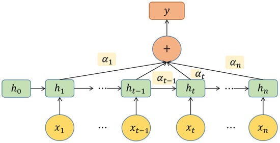
Figure 5.
Flow chart of AM.
In Figure 5, means the input of the BiGRU network, is the output of the hiding layer corresponding to each input through BiGRU, is the probability of AM for the hiding output of BiGRU, and y is the final output of BiGRU in the AM.
To determine the information that is relevant to a given task from N input vectors, , a scoring function is used to calculate the correlation between each input vector and a task-specific representation called the query vector. Starting from a task-related query vector q, we use the attentiveness variable to represent the index location of the retrieved information, i.e., z = n indicates that the Nth input vector was selected. First, given q and X, the probability weight of the ith input vector is calculated, and the output vector of the position hiding layer is used as the input of the AM, and then the corresponding weight is calculated through the formula [20], as shown in (19).
where is the attention distribution and is the attention scoring function. The intention vector is derived from .
Traditional attention mechanisms (AMs) are designed to emulate human cognitive abilities to filter essential information and enhance focus. Here we have incorporated the multi-head attention mechanism (MAM) to capture local features within input sequences and prioritize critical information, thereby refining the model’s interpretative capabilities. The specific architecture of the MAM is depicted in Figure 6.
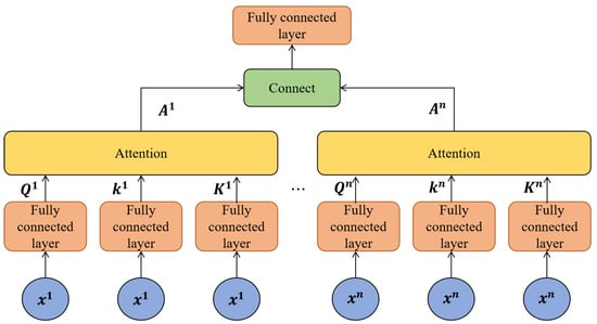
Figure 6.
Flowchart of the multi-head AM.
The operational dynamics of the MAM are initiated by applying multiple parallel linear mappings to the query matrix (Q), key matrix (K), and value matrix (V), enhancing the diversity of the attention perspectives. This process, outlined in Formula (22), allows the MAM to compute attention scores across i distinct attention heads simultaneously, each focusing on different aspects of the input data. The final attention output, termed Multi (Q, K, V), is calculated by aggregating these individual attention head scores, adjusted by a normalization factor from a weight matrix to ensure a balanced contribution. This comprehensive attention computation ensures a nuanced and thorough data interpretation, as detailed further in Formulas (21)–(23).
where is the dimension of matrix Q and K, , , and are the weight matrices of Q, K, and V, respectively, and is the output transformation matrix [30].
2.6. MPA-VMD-BiGRU-MAM Model
Our proposed algorithm, the MPA-VMD-BiGRU-MAM model, is implemented through a structured and integrative approach that harnesses the strengths of each constituent technique to enhance predictive accuracy. The implementation process unfolds as follows:
(1) Data Preprocessing: Initial data preparation involves standard procedures for addressing missing data, outliers, and normalization to ensure data quality and consistency.
(2) Feature Selection: Utilizing the Kendall correlation coefficient, we select significant variables that influence the model, thereby streamlining the input data by removing inconsequential features.
(3) Signal Decomposition with MPA-VMD: The optimized Variational Mode Decomposition (VMD), facilitated by the Marine Predator Algorithm (MPA), decomposes the original time series into its constituent sub-modes. This step is critical as it enhances the model’s ability to handle the inherent fluctuations within the PV power generation data.
(4) Feature Extraction via BiGRU: The decomposed sub-modes are then processed through the Bidirectional Gated Recurrent Unit (BiGRU) to abstract essential temporal characteristics from each sub-mode, capturing dynamic changes over time.
(5) Attention and Integration with MAM: The output from BiGRU serves as the input to the multi-head attention mechanism (MAM), where it undergoes a weighting process. This layer assigns appropriate weights to different features, integrating the predictive insights from various components. The results are then reverse-normalized to translate them back to their original scale, culminating in a unified predictive output.
(6) Model Evaluation and Testing: To ascertain the model’s generalization capabilities and stability across diverse datasets, we employ the Belgian PV power generation dataset as a test case. This allows us to evaluate the model’s performance and investigate the impact of seasonal factors on the PV power forecasting model.
Figure 7 illustrates this comprehensive process, showcasing how each step builds upon the previous to enhance the overall effectiveness and accuracy of the predictive model. By methodically integrating these advanced techniques, the MPA-VMD-BiGRU-MAM model not only achieves superior predictive outcomes but also provides insights into the nuanced dynamics of PV power generation.
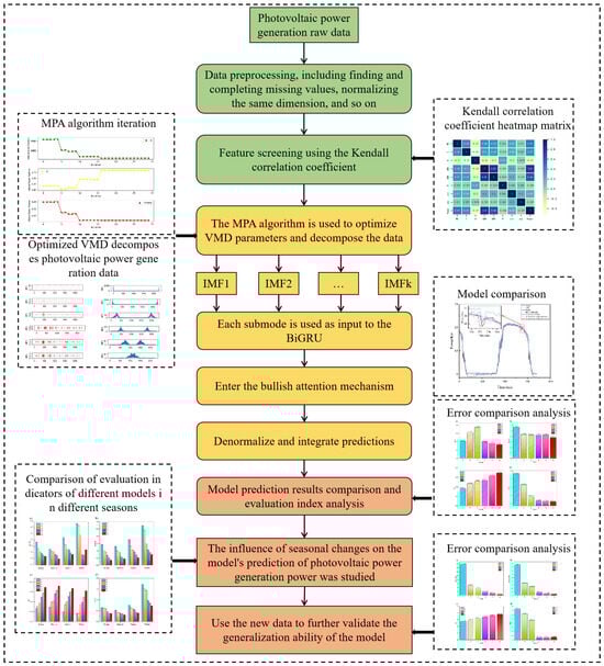
Figure 7.
The framework of our proposed model.
2.7. Assessment Criteria
To quantitatively evaluate the forecasting accuracy of our proposed model and establish a robust comparative benchmark, we employ four key statistical metrics within our model performance evaluation framework. These metrics include Mean Absolute Error (MAE), Root Mean Square Error (RMSE), goodness of fit, and stability (STA). The precise formulations of these indicators are detailed in Equations (23)–(26).
In these equations, and represent the actual and predicted values, respectively, while denotes the mean of the observed data, and symbolizes the variance. Among these metrics, MAE and RMSE are utilized as negative indicators, where lower values signify better model performance. Conversely, goodness of fit and STA are treated as positive indicators, with higher values indicating more favorable outcomes. This dual approach ensures a comprehensive assessment of the model’s accuracy and reliability in capturing and predicting complex patterns within the data.
3. Experimental Analysis
3.1. About the Data
For our experimental analysis, we utilize a comprehensive dataset from the Alice Springs Solar Demonstration Plant in Australia, which encapsulates both operational power outputs and a range of meteorological conditions. The solar PV system under study boasts an installed capacity of 26.52 kW, with data granularity fine-tuned to a 5 min temporal resolution. The dataset encompasses a diverse array of variables including power output (kW), wind speed (m/s), ambient temperature (°C), relative humidity (%), global horizontal radiation (W/m2·sr), diffuse horizontal radiation (W/m2·sr), precipitation levels, and wind direction, which is quantified through its sine and cosine components.
The focus of our analysis narrows to the data collected between 10 June and 20 June 2014, which comprises a total of 2880 data points. We delineate the dataset into training and testing segments, allocating 85% for model training and the remaining 15% for evaluation. The training process was configured with a sliding window of 80 and a batch size of 32, extending over 120 epochs. We experimented with varying the number of neurons in the hidden layers, testing configurations of 32 and 64 neurons to optimize the model performance. Figure 8 provides a visual representation of the raw power generation data, formatted as a bar chart, with time intervals delineated along the x-axis in minutes, days cataloged on the y-axis, and the power output displayed in kilowatt-hours on the z-axis. In this paper, the software used for training data includes the Python(3.10) software used created by Guido van Rossum from Amsterdam, the Netherlands, and the MATLAB(R2021a) software created by Natick from Massachusetts, the United States.
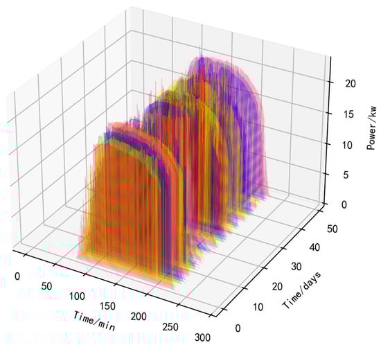
Figure 8.
Original PV power generation.
Table 1 shows some samples.Photovoltaic (PV) power generation is shaped by a variety of environmental factors such as wind speed, temperature, relative humidity, global and diffuse horizontal radiation, precipitation, and the angular components of the wind direction (expressed through sine and cosine terms). Utilizing the Kendall correlation coefficient—a robust measure for evaluating non-parametric relationships—we have delineated these interdependencies within a heat map illustrated in Figure 9, where darker shades signify stronger correlations. Notably, global horizontal irradiance shows a significant positive correlation with PV power generation (coefficient of 0.8), and diffuse horizontal radiation follows closely, with a coefficient of 0.64. Wind speed and relative humidity also influence power output, demonstrating moderate positive and negative correlations, respectively. Meanwhile, lesser impacts are observed from the sine component of wind direction and the cosine components of rainfall and wind direction, the latter two showing only weak correlations with PV power. To optimize our analysis and focus on the most impactful environmental factors, less significant variables have been excluded from further consideration, allowing a streamlined and focused inquiry into those factors most affecting PV power generation.

Table 1.
Part of the sample data.
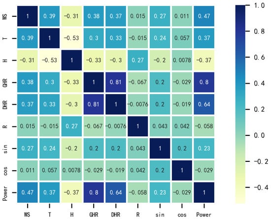
Figure 9.
The heat map of PV power generation variables.
In Figure 9, WS represents wind speed (m/s); T is the ambient temperature (°C); H is the relative humidity (%); GHR stands for global horizontal radiation (W/m2·sr); DHR stands for diffuse horizontal radiation (W/m2·sr); R stands for rainfall; sin refers to the sinusoidal component of the wind direction; and cos is the cosine component of the wind direction.
3.2. VMD Parameter Setting and Optimization
To augment the predictive accuracy of our model, we employ the Marine Predator Algorithm (MPA) to fine-tune the critical parameters within the Variational Mode Decomposition (VMD) framework. Specifically, MPA is used to optimize the number of finite bandwidth mode components (K) and the second-order penalty factor () in the VMD. Alpha here means the same thing as a. According to the historical literature, the number of predators is usually set at 50% of the population size, and the absolute value range is suggested to be between 10 and 50. Dimensions usually range from 10 to 30 dimensions. The value range of the upper/lower boundary is [−10, 10]. The precise settings and values for both the MPA and VMD parameters are systematically outlined in Table 2.
Table 2.
Parameter setting for MPA and VMD.
We have successfully achieved a minimum fitness value of 9.19 after following 30 iterations of the Marine Predator Algorithm (MPA), leading to the identification of the optimal parameter combination [K, ] as [6, 608]. The dynamics of the optimization process are depicted in Figure 10, which illustrates how the MPA stabilizes after 16 iterations. Notably, the second-order penalty factor () remains constant at 608, while the number of finite bandwidth mode components (K) approaches an approximate value of 5.75. Given that K requires an integer value for practical implementation, it is rounded to 6, ensuring both mathematical precision and operational feasibility in the application of VMD. MAE is the MAE value of the benchmark model; is the maximum time allowed; and is the number of model parameters.
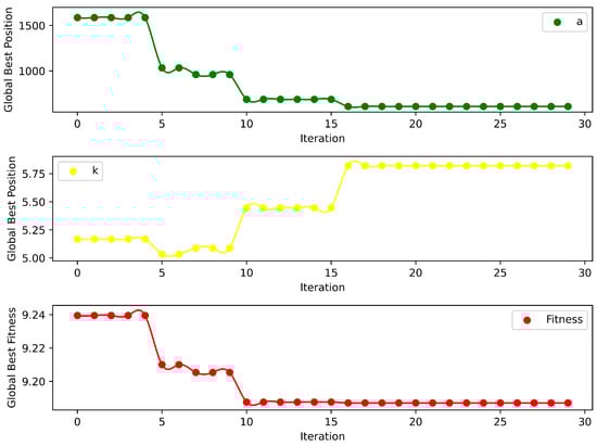
Figure 10.
Parameter iteration in the process of MPA nested in VMD.
3.3. Short-Term PV Prediction via MPA-VMD-BiGRU-MAM
Figure 11 displays the results following the application of MPA-optimized parameters in the VMD process. In Figure 11a, the spectral process of modal components reveals that IMF1 and IMF2 fall into the low-frequency category, while the remaining four are classified as high-frequency ones. Figure 11b highlights the central mode component, demonstrating the independence of each mode and verifying the elimination of mode aliasing, which emphasizes the effectiveness of the carefully optimized VMD parameters in distinguishing the signal into clear and independent modes, a crucial factor for the accurate prediction of PV power generation.
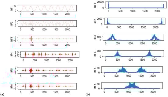
Figure 11.
Solution of VMD: (a) exploded signal diagram and (b) spectrogram.
In the short-term photovoltaic power prediction conducted by us using the MPA-VMD-BiGRU-MAM model, the predicted values and observed values of the first four sub-modes are shown as (a), (b), (c) and (d) in Figure 12 respectively, they showing consistent fluctuations and trends. The correlation coefficients for these modes all exceed 0.97, affirming that our model adeptly captures the overall trend characteristics of the sequence and provides highly accurate predictions of subsequent power generation.
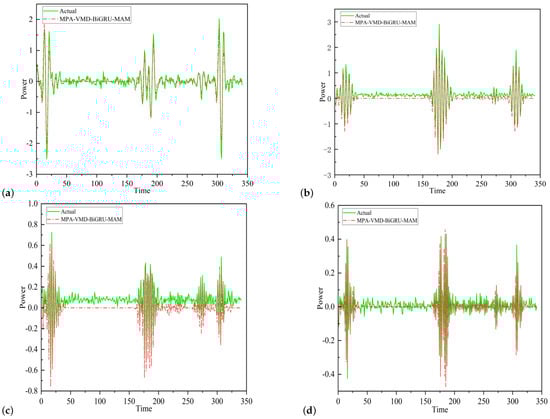
Figure 12.
The sub-mode prediction via MPA-VMD-BiGRU-MAM.
Figures (a), (b), (c) and (d) in Figure 12 reveals slightly divergent fluctuations in the forecast results, suggesting areas for further refinement. After integrating the forecasts from all six modes, the consolidated prediction outcome is displayed in Figure 13. This final result achieves a goodness of fit of 0.9869, with a Mean Absolute Error (MAE) of 0.63, Root Mean Square Error (RMSE) of 1.047, and stability (STA) of 0.9377, which underscore the excellent performance and robustness of our model, highlighting its effectiveness in short-term PV power forecasting.
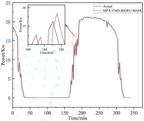
Figure 13.
The fitting trace of the MPA-VMD-BiGRU-MAM model.
To streamline the presentation of various models within our analysis, concise abbreviations for each model have been listed in Table 3. The comparative predictions from all the models have been displayed in Table 4 and Figure 14.
Table 3.
Short names of the models.
Table 4.
Comparison of errors of different models.
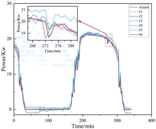
Figure 14.
The prediction of the six models.
It is evident that our model, #6, captured the true curve well, with an MAE of 0.33314, an RMSE of 0.76935, an of 0.97444, and an STA of 0.75161. And model #5 has an of 0.95881 and its STA is 0.85916. The goodness of fit of model #4 is 0.93513, its STA is 0.86309, and the evaluation indexes of the other three models are also known from Table 4. In Figure 15, (a), (b), (c) and (d) respectively represent the MAE value, RMSE value, value, and STA value of the model. As can be seen from Figure 15 illustrates that among the four evaluation indicators, the results of model #6 are the best, which suggests that our model exhibits much better prediction than the other five models.
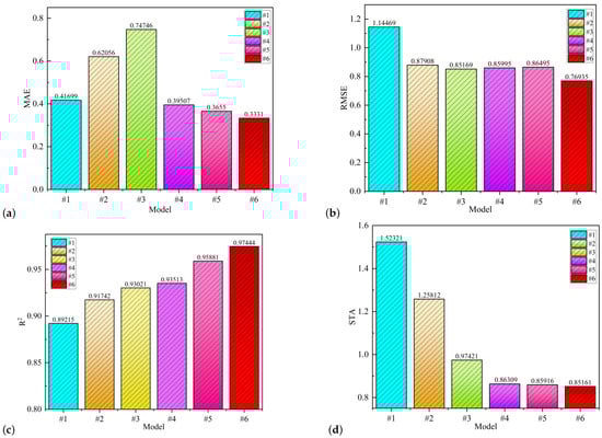
Figure 15.
The errors for the different models.
We have compared the errors of different models, as shown in Figure 15 and Table 4. It is evident that the MAE has decreased from 0.74746 to 0.62056 for model #2 and #1, while the RMSE has decreased from 1.14469 to 0.87908, the STA index has decreased from 1.52321 to 1.25812, and the goodness of fit has increased from 0.89215 to 0.91742. These improvements indicate that the BiGRU model can better capture bidirectional features compared to a single GRU model.
Next, we compare the performance metrics of the MPA-VMD-GRU and MPA-VMD-BiGRU models for models #2 and #1. It can be observed that the VMD technique reduces the complexity and non-linearity of the time series, leading to better predictions. It reduces the MAE of the two models from 0.74746 and 0.62056 to 0.41699 and 0.39507, and improves the goodness of fit from 0.89215 and 0.91742 to 0.93021 and 0.93513, respectively. At the same time, the RMSE and STA metrics decrease, demonstrating the effectiveness and feasibility of using the VMD technique for data decomposition.
Model #5, which includes the multi-head attention mechanism (MAM), shows an MAE of 0.36557, an RMSE of 0.85169, a goodness of fit of 0.95881, and an STA of 0.85916, as shown in Table 4. In comparison, model #6 has an MAE of 0.33314, an RMSE of 0.76935, a goodness of fit of 0.97444, and an STA of 0.75161. These results clearly indicate the significant improvement in forecasting accuracy of our proposed model, highlighting the importance of the MAM step.
3.4. Seasonal Factors in Forecasting PV Power Generation
Seasonal factors exert varying influences on PV power generation. We have selected autumn (March), winter (June), spring (September), and summer (December) as representative seasons. In Figure 16, (a), (b), (c) and (d) respectively calculate the four types of errors of different models and represent them with histographs.It is evident that smaller errors occurred for our proposed model #6, especially during the summer season, demonstrating more accurate predictions.
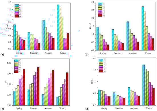
Figure 16.
Comparison of evaluation indexes of different models in different seasons.
Table 5 presents the MAE, RMSE, goodness of fit, and STA values for each model across the four seasons. In terms of prediction accuracy, model #6 consistently outperforms the other five models. For instance, during summer, model #6 achieves an MAE of 0.20197, which is significantly better than the MAE values of 0.5172, 0.4527, 0.4475, 0.34635, and 0.31802 for models #1 to #5, respectively. Similarly, model #6 boasts a goodness of fit of 0.98025, notably surpassing the values for models #1 to #5. The RMSE and STA indicators also demonstrate the robustness of our proposed model across seasons.
Table 5.
Comparison of errors for different models.
3.5. Model Validation
Validation experiments were conducted using an independent dataset derived from PV power plants in Belgium. The dataset is characterized by meteorological and geographical conditions that significantly differ from those in the previously analyzed datasets. Spanning from 1 May to 10 May 2023, the dataset comprises data collected at 15-min intervals, resulting in a total of 960 samples, with power output measured in megawatts. The outcomes of these predictive experiments are visually represented in Figure 17.
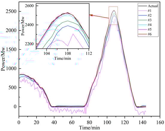
Figure 17.
Predictions from different models.
As depicted in Figure 17, model #6 consistently achieves superior prediction accuracy and exhibits narrower fluctuation intervals relative to the other models tested. Model #5 also performs commendably, maintaining robust results even amidst significant data variability. Notably, model #6 stands out with its exceptional goodness of fit, remaining resilient and reliable under varying conditions. We have conducted a comprehensive comparison of several critical performance metrics to further validate these observations. Figures (a), (b), (c) and (d) of Figure 18 are systematic summaries of all the results of this analysis, and detailed quantitative analyses were conducted in Table 6.
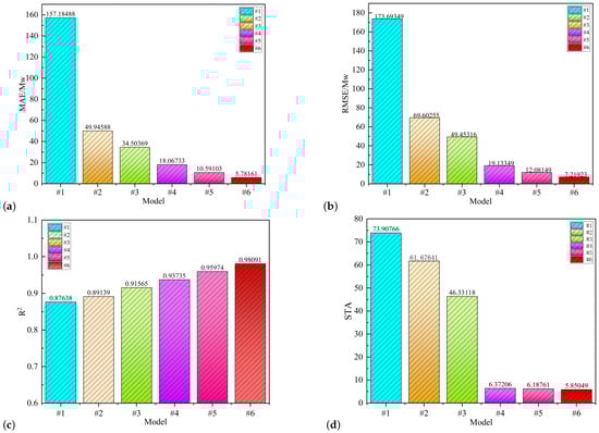
Figure 18.
Different evaluation indexes for different models.
Table 6.
Comparison of errors for different models.
Comparing model #6 to model #1 reveals a substantial improvement: MAE decreases by 96.32%, RMSE decreases by 95.84%, goodness of fit increases by 11.92%, and STA increases by 92.08%. Notably, the significant variation in MAE and RMSE between model #1 and model #2, as shown in Figure 18, underscores the viability of employing the BiGRU model. Additionally, the decline in the STA index from model #3 to model #4 supports the validity of using MPA-VMD in this study. Despite differences in data sampling intervals, numerical units, and data complexity compared to previous datasets, model #6 consistently outperforms other models in terms of predictive performance, demonstrating the robust adaptability of our proposed model.
4. Conclusions
In this research, we developed the MPA-VMD-BiGRU-MAM hybrid model, leveraging sophisticated algorithms to forecast PV power generation with unprecedented accuracy. Through detailed correlation analysis using the Kendall coefficient, we identified pivotal predictors such as global and diffuse horizontal radiation, wind speed, temperature, and the wind direction’s sine angle, which are crucial for enhancing predictive accuracy. The optimization of Variational Mode Decomposition parameters via the Marine Predator Algorithm significantly refined our model’s ability to decompose and analyze PV power data, leading to the superior performance of our proposed model over traditional models. Notably, our model exhibited a reduction in Mean Absolute Error by 38.34% and Root Mean Square Error by 19.6%, alongside improvements in goodness of fit and stability by 4.41% and 33.91%, respectively.
While our model marks a significant step forward in PV power prediction, it also presents opportunities for further refinement. The reliance on substantial computational resources and the limitations of the current dataset, along with the impact of seasonal variations on prediction accuracy, suggest areas ripe for development. Future research will concentrate on enhancing the model’s computational efficiency, expanding the range of environmental and operational variables analyzed, and extending our methodology to broader applications in renewable energy and PV module diagnostics. These efforts are aimed at advancing the precision and utility of PV power forecasting, thereby contributing to the evolution and optimization of renewable energy technologies.
Author Contributions
Y.D. conceived the thesis idea, guidance model, inspection method, revised manuscript, and approved the final draft; S.Z. conducted data follow-up analysis and paper content modification, collected and sorted out materials, implemented research methods and edited manuscripts; W.D. carried out preliminary data analysis and explained the empirical results. All authors have read and agreed to the published version of the manuscript.
Funding
This research received no external funding.
Data Availability Statement
The raw data supporting the conclusions of this article will be made available by the authors on request.
Conflicts of Interest
The authors declare no conflicts of interest.
References
- Vine, E. The Integration of Energy Efficiency, Renewable Energy, Demand Response and Climate Change: Challenges and Opportunities for Evaluators and Planners; Lawrence Berkeley National Laboratory: Berkeley, CA, USA, 2007. [Google Scholar]
- Shi, J.; Lee, W.-J.; Liu, Y.; Yang, Y.; Wang, P. Forecasting power output of photovoltaic systems based on weather classification and support vector machines. IEEE Trans. Ind. Appl. 2012, 48, 1064–1069. [Google Scholar] [CrossRef]
- Vapnik, V. Support-vector networks. Mach. Learn. 1995, 20, 273–297. [Google Scholar]
- Zazoum, B. Solar photovoltaic power prediction using different machine learning methods. Energy Rep. 2022, 8, 19–25. [Google Scholar] [CrossRef]
- Behera, M.K.; Nayak, N. A comparative study on short-term PV power forecasting using decomposition based optimized extreme learning machine algorithm. Eng. Sci. Technol. Int. J. 2020, 23, 156–167. [Google Scholar] [CrossRef]
- Liu, Z.-F.; Luo, S.-F.; Tseng, M.-L.; Liu, H.-M.; Li, L.; Mashud, A.H.M. Short-term photovoltaic power prediction on modal reconstruction: A novel hybrid model approach. Sustain. Energy Technol. Assess. 2021, 45, 101048. [Google Scholar] [CrossRef]
- Guo, G. Transpvp: A transformer-based method for ultra-short-term photovoltaic power forecasting. Energies 2024, 17, 4426. [Google Scholar] [CrossRef]
- Miraftabzadeh, S.M.; Longo, M. High-resolution PV power prediction model based on the deep learning and attention mechanism. Sustain. Energy Grids Netw. 2023, 34, 101025. [Google Scholar] [CrossRef]
- Tang, H.; Kang, F.; Li, X.; Sun, Y. Short-term photovoltaic power prediction model based on feature construction and improved transformer. Energy 2025, 320, 135213. [Google Scholar] [CrossRef]
- Sun, Y.; Yu, H.; Geng, G.; Chen, C.; Jiang, Q. Scalable multi-site photovoltaic power forecasting based on stream computing. IET Renew. Power Gener. 2025, 17, 2379–2390. [Google Scholar] [CrossRef]
- Liu, X.; Liu, Q.; Feng, S.; Ge, Y.; Chen, H.; Chen, C. Novel model for medium to long term photovoltaic power prediction using interactive feature trend transformer. Sci. Rep. 2025, 15, 6544. [Google Scholar] [CrossRef]
- Zhao, X. A novel digital-twin approach based on transformer for photovoltaic power prediction. Sci. Rep. 2024, 14, 26661. [Google Scholar] [CrossRef]
- Wang, C.; Li, M.; Cao, Y.; Lu, T. Gradient boosting dendritic network for ultra-short-term PV power prediction. Front. Energy 2024, 18, 785–798. [Google Scholar] [CrossRef]
- Yang, Y.; Liu, Y.; Zhang, Y.; Shu, S.; Zheng, J. Dest-gnn: A double-explored spatio-temporal graph neural network for multi-site intra-hour pv power forecasting. Appl. Energy 2025, 378, 124744. [Google Scholar] [CrossRef]
- Chen, F.; Ding, J.; Zhang, Q.; Wu, J.; Lei, F.; Liu, Y. A PV Power Forecasting Based on Mechanism Model-Driven and Stacking Model Fusion. J. Electr. Eng. Technol. 2024, 19, 4683–4697. [Google Scholar] [CrossRef]
- Zhu, Y.; Wang, Z.; Zhang, W.; Liu, Y.; Wu, H. A hybrid model for ultra-short-term PV prediction using SOM clustering and ECA. Electr. Eng. 2024, 107, 3349–3358. [Google Scholar] [CrossRef]
- Netsanet, S.; Zheng, D.; Zhang, W.; Teshager, G. Short-term PV power forecasting using variational mode decomposition integrated with Ant colony optimization and neural network. Energy Rep. 2022, 8, 127348. [Google Scholar] [CrossRef]
- Sun, Z.; Zhao, M. Short-term wind power forecasting based on VMD decomposition, ConvLSTM networks and error analysis. IEEE Access 2020, 8, 134422–134434. [Google Scholar] [CrossRef]
- Ospina, J.; Newaz, A.; Faruque, M.O. Forecasting of PV plant output using hybrid wavelet-based LSTM-DNN structure model. IET Renew. Power Gener. 2019, 13, 1087–1095. [Google Scholar] [CrossRef]
- Zhou, H.; Zhang, Y.; Yang, L.; Liu, Q.; Yan, K.; Du, Y. Short-term photovoltaic power forecasting based on long short term memory neural network and attention mechanism. IEEE Access 2019, 7, 78063–78074. [Google Scholar] [CrossRef]
- Ju, Y.; Li, J.; Sun, G. Ultra-short-term photovoltaic power prediction based on self-attention mechanism and multi-task learning. IEEE Access 2020, 8, 44821–44829. [Google Scholar] [CrossRef]
- Yu, M.; Niu, D.; Wang, K.; Du, R.; Yu, X.; Sun, L.; Wang, F. Short-term photovoltaic power point-interval forecasting based on double-layer decomposition and WOA-BiLSTM-Attention and considering weather classification. Energy 2023, 275, 127348. [Google Scholar] [CrossRef]
- Abdi, H. The Kendall rank correlation coefficient. Encycl. Meas. Stat. 2007, 2, 508–510. [Google Scholar]
- Faramarzi, A.; Heidarinejad, M.; Mirjalili, S.; Gandomi, A.H. Marine Predators Algorithm: A nature-inspired metaheuristic. Expert Syst. Appl. 2020, 152, 113377. [Google Scholar] [CrossRef]
- Liang, Z.; Sun, G.; Li, H.; Wei, Z.; Qi, H.; Zhou, Y.; Chen, S. Short-term load forecasting based on VMD and PSO optimized deep belief network. Power Syst. Technol. 2018, 42, 598–606. [Google Scholar]
- Reynolds, A.M.; Frye, M.A. Levy flight movements by honeybees inform algorithms in search optimization. In Proceedings of the International Conference on Computational Science and Its Applications (ICCSA 2014), Guimaraes, Portugal, 30 June–3 July 2014; pp. 123–134. [Google Scholar]
- Yang, J.; Zhou, C.; Li, X.; Pan, A.; Yang, T. A Fault Feature Extraction Method Based on Improved VMD Multi-Scale Dispersion Entropy and TVD-CYCBD. Entropy 2023, 25, 277. [Google Scholar] [CrossRef] [PubMed]
- She, D.; Jia, M. A BiGRU method for remaining useful life prediction of machinery. Measurement 2021, 167, 108277. [Google Scholar] [CrossRef]
- Li, L.-L.; Zhao, X.; Tseng, M.-L.; Tan, R.R. Short-term wind power forecasting based on support vector machine with improved dragonfly algorithm. J. Clean. Prod. 2020, 242, 118447. [Google Scholar] [CrossRef]
- Tong, C.; Zhang, L.; Li, H.; Ding, Y. Temporal inception convolutional network based on multi-head attention for ultra-short-term load forecasting. IET Gener. Transm. Distrib. 2022, 16, 1680–1696. [Google Scholar] [CrossRef]
Disclaimer/Publisher’s Note: The statements, opinions and data contained in all publications are solely those of the individual author(s) and contributor(s) and not of MDPI and/or the editor(s). MDPI and/or the editor(s) disclaim responsibility for any injury to people or property resulting from any ideas, methods, instructions or products referred to in the content. |
© 2025 by the authors. Licensee MDPI, Basel, Switzerland. This article is an open access article distributed under the terms and conditions of the Creative Commons Attribution (CC BY) license (https://creativecommons.org/licenses/by/4.0/).