United Prediction of Travel Modes and Purposes in Travel Chains Based on Multitask Learning Deep Neural Networks

Abstract

Predicting and analyzing travel mode choices and purposes are significant to improve urban travel mobility and transportation planning. Previous research has ignored the interconnection between travel mode choices and purposes and thus overlooked their potential contributions to predictions. Using individual travel chain data collected in South Korea, this study proposes a Multi-Task Learning Deep Neural Network (MTLDNN) framework, integrating RFM (Recency, Frequency, Monetary) to achieve a joint prediction of travel mode choices and purposes. The MTLDNN is constructed to share a common hidden layer that extracts general features from the input data, while task-specific output layers are dedicated to predicting travel modes and purposes separately. This structure allows for efficient learning of shared representations while maintaining the capacity to model task-specific relationships. RFM is then integrated to optimize the extraction of users’ behavioral features, which helps in better understanding the temporal and financial patterns of users’ travel activities. The results show that the MTLDNN demonstrates consistent input variable replacement modes and selection probabilities in generating behavioral replacement patterns. Compared to the multinomial logit model (MNL), the MTLDNN achieves lower cross-entropy loss and higher prediction accuracy. The proposed framework could enhance transportation planning, efficiency, and user satisfaction by enabling more accurate predictions.

1. Introduction

Predicting the travel mode choice and purpose plays crucial roles in transportation planning and travel demand forecasting, as these predictions directly influence the effectiveness and efficiency of transportation systems [1]. A comprehensive understanding of how individuals select travel modes and determine purposes enables transportation planners to design systems that efficiently meet the diverse needs of different user groups. This understanding, in turn, facilitates more informed decisions regarding resource allocation, such as expanding public transit networks, constructing new roads, or enhancing cycling infrastructure [2]. Accurate predictions also contribute to a more efficient transportation system, which reduces traffic congestion, shortens commute times, and enhances travel mobility [3]. Moreover, insights into the travel mode choice and purpose decisions allow policymakers to implement targeted interventions that promote sustainable travel behaviors, such as encouraging public transit use or non-motorized transport options like cycling and walking [4,5]. This approach creates a positive feedback loop, where improvements in mobility options and infrastructure investments further encourage sustainable choices, ultimately reducing environmental impacts and improving urban livability [4].

Purpose selection and mode choice are mutually exclusive, they are not the same as the city area, and the situations are different [6]. Previous studies have often overlooked the possibility of simultaneously predicting both behaviors in travel decision-making [7,8], treating the travel mode choice and purpose prediction as separate research fields. However, for travelers, decisions regarding both the travel mode and destination are typically made concurrently during a single travel [9]. These two factors are inherently interrelated, with the travel mode significantly influencing the destination choice and vice versa. Travel destinations are largely shaped by the travel purpose, and several studies have identified the travel mode as a key variable in predicting the travel purpose, demonstrating that the travel mode choice significantly enhances the accuracy of travel purpose predictions [10,11]. In addition, the selection of a transportation mode by individuals is influenced by their travel purpose. Previous studies have established the critical role of travel purpose in improving the accuracy of travel mode predictions. For example, Cheng et al. (2019) [9] applied a random forest method to forecast the travel mode choice and found that travel purpose ranked fifth in terms of variable importance among 20 input factors. These findings imply that the relationship between the travel mode choice and purpose enhances the model’s predictive power.

Traditionally, the main method for modeling the travel mode choice is the Discrete Choice Model (DCM), which relies on predefined utility norms for each alternative in the selection set [12,13]. The methods for the travel destination prediction can generally be divided into rule-based models (using predefined heuristic rules) and statistical approaches (using logical models). However, statistical methods often struggle with complex data and patterns due to their assumption of linear relationships, which limits their prediction accuracy and performance. In contrast, machine learning (ML) techniques, which can model complex nonlinear relationships, automatically perform feature selection, and adapt flexibly to changes in data, have become increasingly popular for analyzing travel behavior. ML methods have been found to outperform rule-based and statistical methods in predicting travel purposes with higher accuracy [14]. Recent advancements in Multi-Task Learning (MTL) and Deep Neural Networks (DNNs) open up new possibilities for investigating the simultaneous prediction of travel modes and purposes. By utilizing DNNs, it is possible to develop travel mode prediction models tailored to specific travel purposes [15]. MTL allows for the simultaneous prediction of multiple tasks in a single model, for example, the travel mode choice and purpose.

This study introduces a Multi-Task Learning Deep Neural Network (MTLDNN) framework designed to jointly predict travel modes and purposes, addressing critical challenges in travel behavior modeling. By leveraging a shared hidden layer to capture common latent features across tasks and incorporating task-specific layers to account for distinct variations in mode and purpose predictions, the framework enhances generalization through knowledge transfer between related tasks, thereby improving predictive performance compared to single-task models. From a modeling perspective, the MTLDNN integrates deep learning techniques with discrete choice modeling principles, offering a more flexible representation of complex, nonlinear relationships between travel behavior determinants and choice probabilities. Unlike classical Deep Neural Networks (DNNs), which often lack interpretability, and multinomial logit (MNL) models, which may struggle with high-dimensional interactions, the MTLDNN effectively balances predictive accuracy and explainability by structuring the learning process to reflect decision-making dynamics. In terms of data application, the framework is validated using a large-scale travel survey dataset in Seoul, demonstrating its robustness in capturing heterogeneous travel behavior patterns. By learning from diverse trip records, the MTLDNN not only achieves superior prediction accuracy but also offers valuable behavioral insights by elucidating how selection probabilities are influenced by key explanatory variables such as the trip distance, socioeconomic attributes, and available transportation alternatives. These findings highlight the framework’s capacity to provide a more interpretable approach to understanding travel decision-making processes. Overall, the MTLDNN framework presents significant advancements in multi-task learning, deep learning-based travel behavior modeling, and large-scale transportation data analysis, making it a powerful tool for travel demand forecasting, transportation analysis, and policy development [16].

This paper is structured to guide the reader from foundational research to practical applications and final insights. Section 2 reviews the literature on travel pattern and purpose predictions, setting the stage for understanding the current challenges. Section 3 presents an analytical framework with an independence test for travel patterns and purposes, followed by an MTLDNN model. Section 4 applies this framework in a case study, discussing datasets, model performance, and behavioral insights. Section 5 concludes with a summary of the findings, this study’s significance, and future research directions, linking the contributions to broader research and policy contexts.

2. Related Works

For many years, discrete choice models (DCMs) have been extensively employed to model and analyze individual decision-making in transportation, addressing factors such as the mode choice, travel purpose, scheduling, and route selection [17]. Models like Multinomial Logit (MNL), Nested Logit (NL), Cross-Nested Logit (CNL), and Mixed Logit (MXL) possess well-defined mathematical frameworks and offer valuable economic insights into travel behavior [18,19,20,21]. DCMs, for instance, are used to estimate the market shares of travel modes and uncover substitution patterns, which are vital for informing transportation policy. However, the assumptions inherent in these models, such as the independence of irrelevant alternatives (IIA) in MNL, can lead to biased estimates and unreliable predictions when these assumptions are violated. These constraints limit the models’ effectiveness, particularly in the context of complex panel data analysis.

In contrast, machine learning (ML) models have increasingly been adopted in travel behavior research, addressing various quantitative tasks, including car ownership prediction [22], license plate recognition [23], and traffic flow prediction [24]. Notably, ML models have emerged as alternatives to traditional discrete choice models (DCMs) for predicting travel modes [25] and trip purposes [26]. Their key advantage lies in flexibility, as they impose fewer assumptions than DCMs and often achieve higher predictive accuracy. Furthermore, ML models, including support vector machines, classification trees, random forests, and Deep Neural Networks (DNNs), effectively capture nonlinear relationships between variables, a challenge for traditional DCMs. Comparative studies indicate that DNNs consistently outperform DCMs in predicting travel modes and purposes [27,28].

Despite the advantages of ML models in terms of predictive performance, their major drawback is the lack of interpretability compared to DCMs, making it challenging to extract reliable economic information [29]. While some research has demonstrated the feasibility of generating economic insights from DNNs, the reliability of this information is often questioned due to several inherent issues of DNNs, such as sensitivity to hyperparameters, model non-identification, and local irregularities. Consequently, although ML models offer enhanced accuracy, the extraction of interpretable and reliable behavioral insights, which are critical for policy-making, remains a challenge.

Moreover, most existing ML classifiers in travel behavior research are designed for single tasks, such as predicting either the travel mode or travel purpose [30]. This single-task focus limits the generalization ability of these models across different but related tasks. In contrast, MTL offers an optimization by improving generalization across tasks through shared representations and leverages commonalities between tasks by training multiple tasks in parallel, leading to improved prediction performance without sacrificing interpretability. Additionally, MTL helps mitigate the risk of overfitting, as the model is required to find a representation that captures multiple tasks simultaneously [31].

Applying multi-task learning to various applications related to traffic behavior and planning has theoretical and empirical appeal [32]. Multi-task learning refers to learning multiple tasks simultaneously in a model, rather than training a separate model for each task. In the field of traffic behavior and planning, the application of multi-task learning can help us better understand and predict traffic behavior. For example, in terms of car ownership and mode selection, multi-task learning can help predict the car ownership situation of different regions and populations, and combined with mode selection, can help infer the travel patterns of different populations. For example, by combining mode selection, it can be inferred that young people in cities are more inclined to use shared bicycles or public transportation for short travels, while in suburban areas, the probability of households owning private cars is higher.

The MTLDNN adopts the method of constructing Deep Neural Networks, focusing on improving the effectiveness of various independent task combinations and completing multi-task learning. With its strong generalization and pretraining capabilities, along with multi-task learning, the MTLDNN has been successfully applied across various domains, including natural language processing [33,34] and image recognition [35]. In urban analytics, it has been utilized to deduce individual geodemographic characteristics, such as age, gender, income, and car ownership, from public transportation usage patterns [36]. The MTLDNN aligns with the approach of simultaneous estimation in travel behavior studies and shows promise in jointly modeling variables like household car ownership and vehicle kilometers traveled [37], auto ownership and mode choice [38], as well as mode choice alongside psychological or attitudinal factors [39,40]. However, its application in choice modeling remains limited, with the only known instance being its use in the joint modeling of revealed and stated preferences in travel surveys [41]. The multitasking learning ability of the MTLDNN enables the model to handle multiple related tasks simultaneously, providing a more comprehensive understanding of users’ needs [42]. Combined with pretrained models, the MTLDNN can also perform domain adaptation with a small number of labels, improving its generalization ability. At the same time, it can efficiently extract key features, which helps to accurately predict users’ travel habits and destinations. These advantages make the MTLDNN a powerful tool for travel prediction in intelligent transportation systems.

Although there have been some individual prediction studies on travel patterns or destinations, there is still relatively little comprehensive research on the joint prediction of travel patterns and destinations [43]. Especially when considering multiple modes of transportation, multiple travel scenarios, and data sparsity, accurately predicting travel patterns and destinations remains a challenge. This gap in research highlights the need for further exploration of MTLDNNs in travel behavior analyses. Therefore, this study aims to address this gap by employing a classical MTLDNN architecture to jointly predict travel modes and purposes. This approach not only enhances the predictive accuracy but also retains the ability to generate interpretable economic information, thereby overcoming the limitations of both traditional DCMs and existing ML models.

3. Methods

The research framework is illustrated in Figure 1. Pearson’s chi-square test is first applied to assess the independence between the travel mode and trip purpose in the survey data. Identifying whether these variables are correlated or independent is crucial for data analysis. If they are independent, predicting one does not require considering the other. However, a significant correlation necessitates incorporating both in predictive modeling. Since the travel mode and trip purpose are categorical variables, Pearson’s chi-square test is an appropriate method for evaluating their independence.

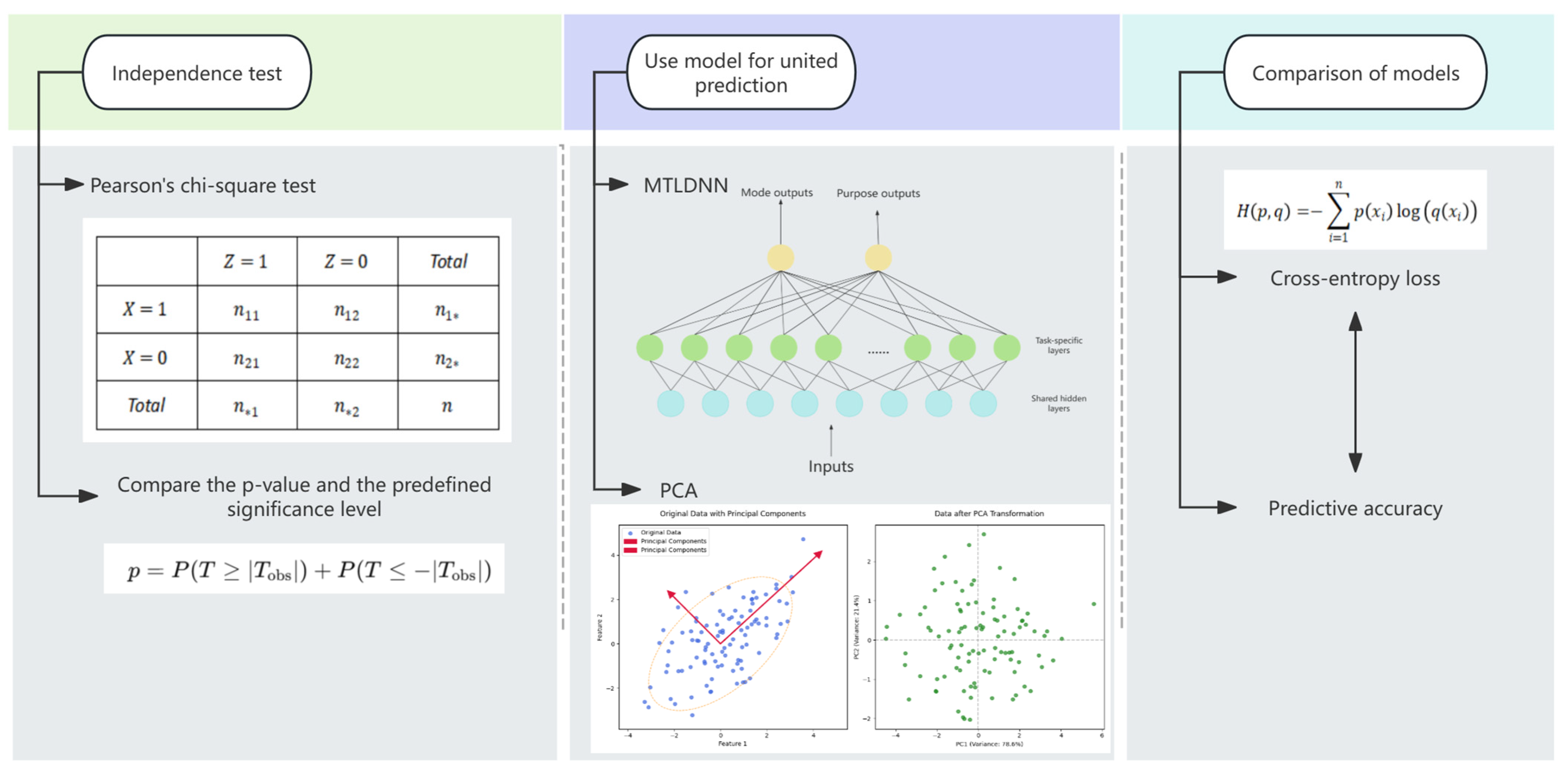
Subsequently, data analysis is conducted using the MTLDNN framework along with other relevant models. The application of the MTLDNN framework and related models enables a deeper understanding of the underlying patterns and characteristics within the data, thereby providing robust support for subsequent predictive tasks. Additionally, the model-based analysis facilitates the identification of potential anomalies and inconsistencies in the data, allowing for targeted adjustments and refinements.

Finally, comparing the prediction results through cross entropy loss and accuracy measurements can comprehensively evaluate the performance of the model. Cross entropy loss reflects the loss situation of the model in the prediction process, while accuracy directly reflects the prediction accuracy of the model. Combining these two indicators can provide a more comprehensive understanding of the performance of the model.

3.1. Independence of the Travel Mode and Purpose

Pearson’s chi-square test is a common method for hypothesis testing, particularly for evaluating the independence of categorical variables. It constructs a contingency table to represent the multivariate frequency distribution of the variables. Given mode and purpose choices with dimensions $K_m$ and $K_p$, respectively, and $O_{ij}$ as the observed frequency of mode $i$ and purpose $j$, the chi-square test statistic is calculated as follows:

$$X^2=\sum _{i=1}^{K_m}\sum _{j=1}^{K_p}{\displaystyle \frac{{\left({O_{ij}-E}_{ij}\right)}^2}{E_{ij}}}$$

(1)

where $E_{ij}$ represents the expected frequency of mode $i$ and purpose $j$ under the null hypothesis of independence.

The p-value is derived by comparing the test statistic to the chi-square distribution. If the p-value is lower than the specified significance level, the null hypothesis is rejected. In this study, a significance level of 0.01 is applied, meaning that a p-value below 0.01 signifies a statistically significant relationship between the travel mode and purpose.

3.2. Multitask Learning Deep Neural Network for the Mode and Purpose

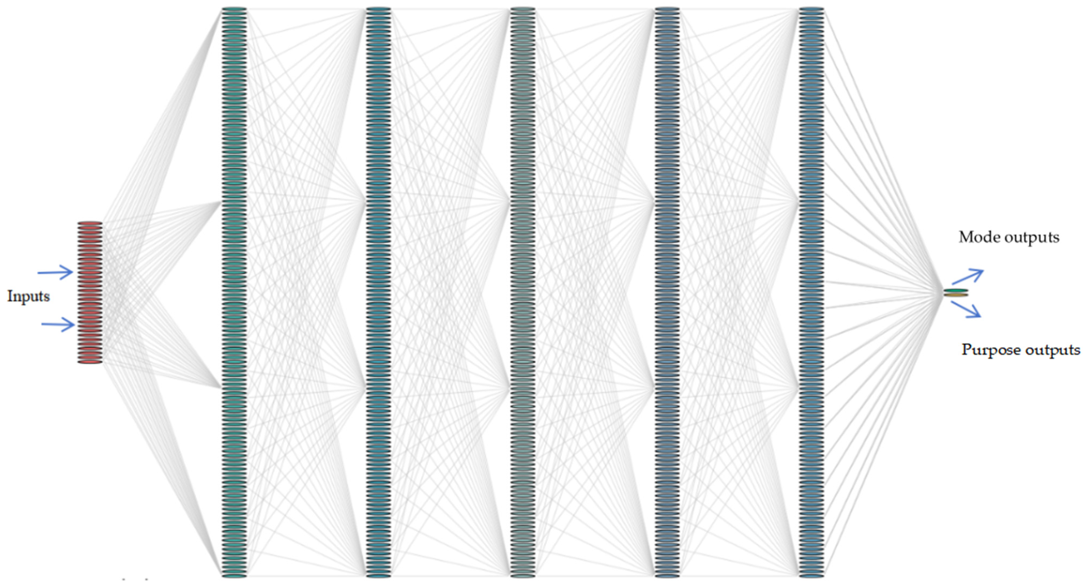
The structure of the MTLDNN model is shown in Figure 2.

The MTLDNN model is optimized using empirical risk minimization (ERM), incorporating both classification errors and regularization terms:

$$\begin{gathered} \underset{w_m,w_p,w_0}{\mathit{min}}R\left(X,Y;w_m,w_p,w_0;c_H\right)=\underset{w_m,w_p,w_0}{\mathit{min}}\left\{{\theta }_m\times \widehat{L_M}\left(w_m,w_0\right)+{\theta }_p\times \widehat{L_P}\left(w_p,w_0\right)+{\lambda }^{T}g\left(w_m,w_p,w_0\right)\right\} \\ =\underset{w_m,w_p,w_0}{\mathit{min}}\left\{-{\displaystyle \frac{{\theta }_m}{N}}{\sum }_{i=1}^{N_x}{\sum }_{j=1}^{K_m}{y}_{m,i}\left[j\right]\mathit{log}P\left(y_{m,i}\left[j\right];w_m,w_0;c_H\right) \\ -{\displaystyle \frac{{\theta }_p}{N}}{\sum }_{i=1}^{N_x}{\sum }_{j=1}^{K_p}{y}_{p,i}\left[j\right]\mathit{log}P\left(y_{p,i}\left[j\right];w_p,w_0;c_H\right)+{\lambda }_1\left(‖w_0‖+‖w_m‖+‖w_p‖\right) \\ +{\lambda }_2\left({‖w_0‖}_2^2+{‖w_m‖}_2^2+{‖w_p‖}_2^2\right)\right\} \end{gathered}$$

(2)

The MTLDNN framework for analyzing mode and purpose is structured as follows. Let $x_i \in R^d$ represent the input variables associated with mode and purpose, where $i \in \{1, 2, \cdots , N\}$ indexes the observations and $\mathrm{d}$ denotes the input dimension. The respective output choices for the mode and purpose are denoted as $y_{m,i}$ and $y_{p,i}$, with $y_{m,i}\in {\left\{\mathrm{0,1}\right\}}^{K_m}$ and $y_{p,i}\in {\left\{\mathrm{0,1}\right\}}^{K_p}$ referring to the mode and purpose, respectively. Here, $K_m$ and $K_p$ define the dimensions of mode and purpose choices, respectively, and both $y_{m,i}$ and $y_{p,i}$ are expressed as binary vectors. Given the constraint that only one alternative for mode or purpose selection can be valid at a time, their feature transformations are formulated in Equations (3) and (4):

$$V_{m,i}={\left(g_m^{M_2}\circ g_m^{M_2-1}\circ ...\circ g_m^1\right)}^{°}\left(g_0^{M_1}\circ g_0^{M_1-1}\circ ...\circ g_0^1\right)\left(x_{m,i}\right)$$

(3)

$$V_{p,i}={\left(g_p^{M_2}\circ g_p^{M_2-1}\circ ...\circ g_p^1\right)}^{°}\left(g_0^{M_1}\circ g_0^{M_1-1}\circ ...\circ g_0^1\right)\left(x_{p,i}\right)$$

(4)

where $M_1$ denotes the depth of shared layers, while $M_2$ denotes the depth of the task-specific (non-shared) layers for each individual task. The transformation of a single shared layer is denoted as $g_0$, whereas $g_m$ and $g_p$ correspond to the transformations of individual layers in the mode and purpose tasks, respectively. With the exception of the output layer, all transformation functions—including $g_m$, $g_p$, and $g_0$—consist of a ReLU activation followed by a linear transformation, expressed as $g^l\left(x\right)=max\left\{W^{l}x,0\right\},\forall l\ne M_2$. The overall MTLDNN architecture is outlined in Equations (2) and (3) and visually represented in Figure 1, where $\left(g_0^{M_1}\circ g_0^{M_1-1}\circ ...\circ g_0^1\right)$ signifies the shared layers, and $\left({\mathrm{g}}_{\mathrm{m}}^{{\mathrm{M}}_2}\circ {\mathrm{g}}_{\mathrm{m}}^{{\mathrm{M}}_2-1}\circ ...\circ {\mathrm{g}}_{\mathrm{m}}^1\right)$ and $\left({\mathrm{g}}_{\mathrm{p}}^{{\mathrm{M}}_2}\circ {\mathrm{g}}_{\mathrm{p}}^{{\mathrm{M}}_2-1}\circ ...\circ {\mathrm{g}}_{\mathrm{p}}^1\right)$ correspond to the task-specific layers for mode and purpose analyses, respectively. The probability distributions for mode and purpose choices are determined using a standard softmax activation function, which is widely applied in multi-class classification, as shown below.

$$P\left(y_{m,i}\left[k\right];w_m,w_0\right)={\displaystyle \frac{e^{V_{m,i}\left[k\right]}}{{\sum }_{j=1}^{K_m}{e}^{V_{m,i}\left[j\right]}}}$$

(5)

$$P\left(y_{p,i}\left[k\right];w_p,w_0\right)={\displaystyle \frac{e^{V_{p,i}\left[k\right]}}{{\sum }_{j=1}^{K_p}{e}^{V_{p,i}\left[j\right]}}}$$

(6)

where ${\mathrm{w}}_{\mathrm{m}}$ and ${\mathrm{w}}_{\mathrm{p}}$ represent the task-specific parameters in ${\mathrm{g}}_{\mathrm{m}}$ and ${\mathrm{g}}_{\mathrm{p}}$; and ${\mathrm{w}}_0$ represents the shared parameters in ${\mathrm{g}}_0$. Equation (5) computes the choice probability for each of the ${\mathrm{K}}_{\mathrm{m}}$ mode alternatives, and Equation (6) computes the probability of each of the ${\mathrm{K}}_{\mathrm{p}}$ travel purposes, given the input data.

The main equation consists of four parts. The first two parts are shown as follows:

$$\widehat{L_M}\left(w_m,w_0\right)=-{\displaystyle \frac{{\theta }_m}{N}}{\sum }_{i=1}^{N_x}{\sum }_{j=1}^{K_m}{y}_{m,i}\left[j\right]\mathit{log}P\left(y_{m,i}\left[j\right];w_m,w_0;c_H\right)$$

(7)

$$\widehat{L_P}\left(w_p,w_0\right)=-{\displaystyle \frac{{\theta }_p}{N}}{\sum }_{i=1}^{N_x}{\sum }_{j=1}^{K_p}{y}_{p,i}\left[j\right]\mathit{log}P\left(y_{p,i}\left[j\right];w_p,w_0;c_H\right)$$

(8)

These terms represent the empirical risk associated with predicting the mode and purpose, both formulated as cross-entropy loss functions. The third component, ${\lambda }_1\left(‖w_0‖+‖w_m‖+‖w_p‖\right)$, corresponds to the L1-class regularization term with an associated weight ${\lambda }_1$, where $‖w_0‖={\sum }_j\left|w_{0,j}\right|$. Similarly, the fourth component, ${\lambda }_2\left({‖w_0‖}_2^2+{‖w_m‖}_2^2+{‖w_p‖}_2^2\right)$, denotes the L2-class regularization term, weighted by ${\lambda }_2$, where ${‖w_0‖}_2^2={\sum }_j{w}_{0,j}^2$. Equation (5) integrates four hyperparameters $\left({\theta }_m,{\theta }_p,{\lambda }_1,{\lambda }_2\right)$, subject to the constraint ${\theta }_m+{\theta }_p=1$. Specifically, ${\theta }_m$ and ${\theta }_p$ control the relative importance assigned to mode and purpose prediction, while ${\lambda }_1$ and ${\lambda }_2$ regulate the overall magnitudes of the layer weights. Larger ${\lambda }_1$ and ${\lambda }_2$ result in greater weight decay during the Deep Neural Network training process.

When analyzing multivariate data, the complexity of variable correlations and the increased effort required for data collection often make it challenging to isolate individual indicators in a way that fully captures the inherent relationships between variables, potentially leading to incomplete or biased conclusions. On the other hand, overly simplifying the analysis by reducing the number of indicators, while convenient, may result in the loss of critical information, ultimately leading to inaccurate conclusions. Thus, it is imperative to maintain a balance between analytical efficiency and the retention of the original information.

3.3. Integrating Principal Component Analysis (PCA) and RFM (Recency, Frequency, Monetary)

In this study, Principal Component Analysis (PCA) is employed to systematically transform highly correlated variables into a smaller set of uncorrelated variables. These newly derived variables serve as comprehensive indicators, independently representing different aspects of the original data, thereby simplifying the dataset while maximizing the preservation and utilization of key information. If the dataset is n-dimensional and consists of m data points $\left({\mathrm{x}}^{\left(1\right)},{\mathrm{x}}^{\left(2\right)},{\mathrm{x}}^{\left(3\right)},...,{\mathrm{x}}^{\left(\mathrm{m}\right)}\right)$, the dimensionality of these m data is expected to be reduced from n-dimensional to k-dimensional, hoping that these m k-dimensional datasets can represent the original dataset as much as possible.

From the above two sections, we can see that finding the n-dimensional principal components of sample ${\mathrm{x}}^{\left(\mathrm{i}\right)}$ is actually finding the covariance matrix $\mathrm{X}{\mathrm{X}}^{\mathrm{T}}$ of the sample set, where the first n’ eigenvalues correspond to the eigenvector matrix $\mathrm{W}$, and then for each sample ${\mathrm{x}}^{\left(\mathrm{i}\right)}$, perform the following transformation ${\mathrm{z}}^{\left(\mathrm{i}\right)}={\mathrm{W}}^{\mathrm{T}}{\mathrm{x}}^{\left(\mathrm{i}\right)}$ to achieve the PCA goal of dimensionality reduction.

The following is the specific algorithm process (Algorithm 1):

Algorithm 1: Principal Component Analysis (PCA)

1. Initialize centered data matrix ${\mathrm{X}}_{\mathrm{c}\mathrm{e}\mathrm{n}\mathrm{t}\mathrm{e}\mathrm{r}\mathrm{e}\mathrm{d}}\leftarrow \mathrm{X}-1{\mathrm{\mu }}^{\mathrm{T}}$, where $\mathrm{\mu }$ is the mean vector.

2. for each feature pair $(\mathrm{i},\mathrm{j})$ do

$\hspace{1em}\hspace{1em}\hspace{1em}\hspace{1em}\hspace{1em}\hspace{1em}\hspace{1em}\hspace{1em}\hspace{1em} {\mathrm{C}}_{\mathrm{i},\mathrm{j}}\leftarrow {\displaystyle \frac{1}{\mathrm{m}}}\sum _{\mathrm{k}=1}^{\mathrm{m}}{\mathrm{X}}_{\mathrm{c}\mathrm{e}\mathrm{n}\mathrm{t}\mathrm{e}\mathrm{r}\mathrm{e}\mathrm{d}}^{\left(\mathrm{k},\mathrm{i}\right)}{\mathrm{X}}_{\mathrm{c}\mathrm{e}\mathrm{n}\mathrm{t}\mathrm{e}\mathrm{r}\mathrm{e}\mathrm{d}}^{\left(\mathrm{k},\mathrm{j}\right)}$

4. end for

5. Compute eigenvalue decomposition of $\mathrm{C}$:

$\hspace{1em}\hspace{1em}\hspace{1em} \left[\mathrm{V},\mathrm{\Lambda }\right]\leftarrow \mathrm{E}\mathrm{i}\mathrm{g}\mathrm{e}\mathrm{n}\mathrm{D}\mathrm{e}\mathrm{c}\mathrm{o}\mathrm{m}\mathrm{p}\left(\mathrm{C}\right),\mathrm{w}\mathrm{h}\mathrm{e}\mathrm{r}\mathrm{e} \mathrm{\Lambda }=\mathrm{d}\mathrm{i}\mathrm{a}\mathrm{g}\left({\mathrm{\lambda }}_1,...,{\mathrm{\lambda }}_{\mathrm{n}}\right)$

7. Sort eigenvectors in $\mathrm{V}$ by descending eigenvalues ${\mathrm{\lambda }}_{\mathrm{i}}$.

8. for $\mathrm{t}\leftarrow 1$ to $\mathrm{n}\mathrm{\prime }$ do

9. $\hspace{1em}\hspace{1em}\hspace{1em}\hspace{1em}\hspace{1em}\hspace{1em}\hspace{1em}\hspace{1em}\hspace{1em} {\mathrm{W}}_{:,\mathrm{t}}\leftarrow {\mathrm{V}}_{:,\mathrm{t}}$(Select top $\mathrm{n}\mathrm{\prime }$ components)

10. end for

11. for each sample ${\mathrm{x}}_{\mathrm{i}}$ do

Input—n-dimensional sample set $\mathrm{D}=\left({\mathrm{x}}^{\left(1\right)},{\mathrm{x}}^{\left(2\right)},{\mathrm{x}}^{\left(3\right)},...,{\mathrm{x}}^{\left(\mathrm{m}\right)}\right)$, the dimensions are to be reduced to n’.

Output—reduced dimensional sample set $\mathrm{D}\prime$;

(1) Centralize all samples$—{\mathrm{x}}^{\left(\mathrm{i}\right)}={\mathrm{x}}^{\left(\mathrm{i}\right)}-{\displaystyle \frac{1}{\mathrm{m}}}\sum _{\mathrm{j}=1}^{\mathrm{m}}{\mathrm{x}}^{\left(\mathrm{j}\right)}$;

(2) Calculate the covariance matrix $\mathrm{X}{\mathrm{X}}^{\mathrm{T}}$ of the sample;

(3) Perform eigenvalue decomposition on matrix $\mathrm{X}{\mathrm{X}}^{\mathrm{T}}$;

(4) Extract the eigenvectors $\left({\mathrm{w}}_1,{\mathrm{w}}_2,...,{\mathrm{w}}_{\mathrm{n}\prime }\right)$corresponding to the largest n’ eigenvalues, standardize all eigenvectors, and form the eigenvector matrix $\mathrm{W}$;

(5) Convert each sample ${\mathrm{x}}^{\left(\mathrm{i}\right)}$ in the sample set into a new sample ${\mathrm{z}}^{\left(\mathrm{i}\right)}={\mathrm{W}}^{\mathrm{T}}{\mathrm{x}}^{\left(\mathrm{i}\right)}$;

(6) Obtain the output sample set $\mathrm{D}\prime =\left({\mathrm{z}}^{\left(1\right)},{\mathrm{z}}^{\left(2\right)},{\mathrm{z}}^{\left(3\right)},...,{\mathrm{z}}^{\left(\mathrm{m}\right)}\right)$.

The Recency, Frequency, Monetary (RFM) model is a widely utilized analytical framework in marketing and customer relationship management (CRM) for assessing customer value and behavioral characteristics [44]. By incorporating three key dimensions—Recency (R), Frequency (F), and Monetary (M)—the model enables businesses to segment customers based on their purchasing behavior and engagement patterns. The underlying assumption of the RFM model is that customers who have made recent purchases, buy frequently, and spend more are more valuable and likely to continue engaging with the business. Consequently, RFM analysis serves as a fundamental approach for customer segmentation, personalized marketing, customer churn prediction, and strategic decision-making in various industries such as retail, e-commerce, finance, and telecommunications.

The RFM model is based on three distinct yet interrelated metrics. Recency (R) measures the time elapsed since a customer’s most recent purchase, typically expressed in days, weeks, or months. A lower recency value suggests a more active customer, whereas a higher value may indicate disengagement or potential churn. It is calculated as follows:

$$\mathrm{R}\mathrm{S}=\mathrm{C}\mathrm{u}\mathrm{r}\mathrm{r}\mathrm{e}\mathrm{n}\mathrm{t} \mathrm{D}\mathrm{a}\mathrm{t}\mathrm{e}-\mathrm{M}\mathrm{o}\mathrm{s}\mathrm{t} \mathrm{R}\mathrm{e}\mathrm{c}\mathrm{e}\mathrm{n}\mathrm{t} \mathrm{P}\mathrm{u}\mathrm{r}\mathrm{c}\mathrm{h}\mathrm{a}\mathrm{s}\mathrm{e} \mathrm{D}\mathrm{a}\mathrm{t}\mathrm{e}$$

(9)

Frequency (F) represents the number of purchases made by a customer within a specified time period, serving as an indicator of customer loyalty and engagement. Higher frequency values suggest that a customer has a strong relationship with the business. This metric is computed as follows:

$$\mathrm{F}\mathrm{S}=\mathrm{T}\mathrm{o}\mathrm{t}\mathrm{a}\mathrm{l} \mathrm{N}\mathrm{u}\mathrm{m}\mathrm{b}\mathrm{e}\mathrm{r} \mathrm{o}\mathrm{f} \mathrm{P}\mathrm{u}\mathrm{r}\mathrm{c}\mathrm{h}\mathrm{a}\mathrm{s}\mathrm{e}\mathrm{s} \mathrm{i}\mathrm{n} \mathrm{a} \mathrm{G}\mathrm{i}\mathrm{v}\mathrm{e}\mathrm{n} \mathrm{P}\mathrm{e}\mathrm{r}\mathrm{i}\mathrm{o}\mathrm{d}$$

(10)

Monetary (M) quantifies the total expenditure of a customer over a given timeframe, reflecting their overall contribution to revenue. Customers with high monetary values are typically prioritized for retention and targeted promotions. It is calculated as follows:

$$MS=\sum (Transaction Amounts Over the Defined Period)$$

(11)

To facilitate customer segmentation, RFM scores are often assigned to each dimension, ranking customers into quartiles or percentile groups. These scores are then combined to categorize customers into distinct groups, such as high-value loyal customers, at-risk customers, and low-engagement customers.

Sometimes, we do not specify the value of n’ after dimensionality reduction, but instead specify a principal component weight threshold t for dimensionality reduction. This threshold $\mathrm{t}$ is between $(0,1]$. If n eigenvalues are ${\lambda }_1\ge {\lambda }_2\ge ...\ge {\lambda }_{\mathrm{n}}$, then n’ can be obtained by the following equation:

$${\displaystyle \frac{\sum _{i=1}^{n\prime }{\lambda }_i}{\sum _{i=1}^n{\lambda }_i}}\ge t$$

(12)

$$RFM=RS\times 100+FS\times 10+MS\times 1$$

(13)

The RFM model offers several advantages. First, it is computationally simple and relies solely on transaction data, making it easy to implement and interpret. Second, it provides strong explanatory power for customer behavior by segmenting customers based on tangible purchasing patterns. Third, it is widely applicable across multiple industries, including retail, banking, and subscription-based services. However, the model also has limitations, such as its static nature and its reliance solely on transaction history, excluding behavioral attributes like product preferences or browsing history. To enhance its effectiveness, the RFM model can be integrated with machine learning techniques such as clustering algorithms (e.g., K-Means) for more granular segmentation or extended to a dynamic RFM (d-RFM) approach, incorporating time-weighted recency metrics to track changes in customer behavior over time. Overall, the RFM model remains a valuable tool for businesses seeking to optimize customer engagement strategies, predict churn, and enhance targeted marketing campaigns.

4. Data Source and Experiment Setup

4.1. Datasets

The public transportation system in South Korea is highly advanced and efficient, and is characterized by a comprehensive network of buses, subways, and trains. Major cities, such as Seoul, Busan, and Incheon, are served by modern and well-maintained subway systems that provide frequent and reliable services. The bus network is equally extensive, covering urban, suburban, and rural regions with diverse routes. Additionally, high-speed trains connect major cities, enabling rapid and convenient travel across the country. Integrated fare systems, along with technological innovations such as real-time tracking and mobile payment platforms, further enhance the accessibility and convenience of South Korea’s public transportation.

The dataset employed in this study consists of travel node data for travelers within various administrative regions of Seoul, South Korea, including details on departure locations, public transportation boarding and alighting stations, transfer points, and the time and location of arrivals. A total of 959,367 travel chain samples were extracted from the travel origin–destination (OD) data of travelers from January to November 2020, which were designated as the training set. The travel OD data collected in December 2020 were used as the test set for predicting travel chains. Each travel chain sample contains information on the travel region, travel time, destination, travel cost, and mode of transportation, as detailed in

Table 1. Data labels and explanations.

Name	Explanation	Example
Area	Administrative district	Yangsan
Personal ID	ID representing identity	P011442072
T start	Departure time from origin	20210228181829
T arrival	Time to destination	20210228184829
P start	Departure location	35.23, 129.09
P arrival	Place of arrival	35.34, 129.02
T travel	Boarding time	20210228181829
T alight	Time to get off	20210228184829
ID travel	Boarding station ID	49981
ID alight	Drop off site ID	49815
N travel	Boarding station name	Ankang Sandaocheng
N alight	Drop off site name	POSCO 2 doors
P travel	Boarding station coordinate	35.37, 129.15
P alight	Drop off site coordinate	35.99, 129.39
Trans	Transport mode	Bus
Cost	Fare	KRW 2080

.

The data were collected from volunteers and record their location and time information for boarding and alighting from various transportation modes, as well as transfer points. An example of the travel process for one volunteer is illustrated in Figure 3, which includes four modes of transportation: walking, bicycling, bus, and subway.

The data on traveler movements were systematically collected through a volunteer-based methodology. Participants were recruited via established social channels, including community announcements and digital platforms, and were provided with GPS-enabled devices to record spatiotemporal data at critical trip stages—namely, departure (time and location), transfer points, and arrival (time and location) [45]. Complementary attributes, such as land-use classification at nodal points, travel mode, and trip cost, were obtained through an accompanying survey application. To ensure temporal representativeness, data collection encompassed peak hours (6:00–9:00 and 16:00–19:00), off-peak periods, and weekends, with targeted sampling in urban zones exhibiting a high active travel demand. Rigorous quality control measures were implemented: raw GPS trajectories were cross-validated against survey responses, and non-plausible features (e.g., impossible speeds or incomplete nodal data) were systematically excluded. The study strictly adhered to ethical research standards for all participants before data collection and surveys. This methodological framework aligns with practices in travel behavior research, thereby safeguarding both the validity and reliability of the resultant dataset.

Due to a small portion of missing station data, bus stop matching methods were employed to impute missing alighting station information (Barry et al., 2002 [46]).

Based on existing data, the travel modes are divided into four categories, walking, bicycle, bus, and subway, with the corresponding serial numbers shown in

Table 2. Travel mode and corresponding number.

Number	Mode
1	Walking
2	Bicycle
3	Bus
4	Subway

.

The corresponding travel chain types (transfer types) and corresponding number of travel chains in the extracted data are shown in

Table 3. Transfer type and number of travel chains.

Transfer Type	Number of Travels
1-3-3	145,276
1-3-4	138,642
2-3-3	97,102
2-3-4	90,063
1-3	125,683
1-4	72,570
2-3	39,826
2-4	32,584
…	…

.

Selected variables include the start and end time, duration, and land use characteristics around the activity location [47]. This means that researchers considered these key factors when analyzing activities, such as the time span of the activity and the land use around the location. For example, one activity may last for several hours and occur in a commercial area, while another activity may last for a whole day and occur in a residential area. The selection of these variables can help determine the characteristics and impact of the activity. The government also provides POI (Point of Interest) information for each building, which includes different types such as residential, commercial, and office buildings. These pieces of information will help determine the characteristics of the activity location and the impact of the surrounding environment [48].

Then, in order to match land use information to travel chain, we first divide land use into four initial parts: residential areas, commercial areas, work areas, and other areas. For the residential areas, we further categorize them into three levels, high-density areas, low-density areas, and ordinary areas, and divide commercial areas into two levels: high-density areas and low-density areas.

4.2. Experiment Setup

This study seeks to evaluate the performance of MTLDNNs in comparison to Single-Task Learning Deep Neural Networks (STLDNNs) and benchmark models, namely, the Multinomial Logit Model (MNL). In training deep neural network models, the careful selection of hyperparameters, which define the model architecture and regularization, is crucial, as model performance is highly sensitive to these parameters. To this end, the hyperparameter space was predefined (see

Table 4. Hyperparameter space of the MTLDNN.

Hyperparameter	Values
Number of shared layers	$\left[\mathrm{2,3},4\right]$
Number of task-specific layers	$\left[\mathrm{1,2}\right]$
${\lambda }_1$ constant	$1^{-20}$
${\lambda }_2$ constant	$1^{-10}$
${\mathrm{\theta }}_{\mathrm{m}}$	$\left[\mathrm{0.05,0.5,0.95}\right]$
Learning rate	0.001
Batch size	200

), and an exhaustive grid search was conducted to identify the optimal hyperparameters. Model performance was assessed using a holdout validation method, whereby the original survey data were split into a training set and a testing set with a ratio of 7:3. The training set was utilized for model training, while the testing set was reserved for evaluating model performance.

4.3. MNLs for Mode and Purpose

This study evaluates the performance of Deep Neural Networks (DNNs) in analyzing mode and purpose by comparing them with two baseline Multinomial Logit (MNL) models, each dedicated to mode and purpose predictions. For clarity, the MNL model for mode prediction is referred to as MNL-M, while the one for purpose prediction is denoted as MNL-P. The utility function for MNL-M is structured linearly as follows:

$${\mathrm{U}}_{\mathrm{m},\mathrm{i}}={\mathrm{V}}_{\mathrm{m},\mathrm{i}}+{\mathrm{\epsilon }}_{\mathrm{m},\mathrm{i}}={\mathrm{w}}_{\mathrm{m}}^{\mathrm{T}}{\mathrm{x}}_{\mathrm{m},\mathrm{i}}+{\mathrm{\epsilon }}_{\mathrm{m},\mathrm{i}}$$

(14)

where ${\mathrm{w}}_{\mathrm{m}}$ is the parameter for the travel mode analysis; ${\mathrm{\epsilon }}_{\mathrm{m},\mathrm{i}}$ epsilon is the random utility term, and ${\mathrm{x}}_{\mathrm{m},\mathrm{i}}$ denotes the independent variables for mode choice.

Following this, the choice probability function for each of the ${\mathrm{K}}_{\mathrm{m}}$ mode alternatives in discrete choice models (DCMs) is calculated as follows:

$$\mathrm{P}\left({\mathrm{y}}_{\mathrm{m},\mathrm{i}}\left[\mathrm{k}\right];{\mathrm{w}}_{\mathrm{m}}\right)={\displaystyle \frac{{\mathrm{e}}^{\left[{\mathrm{w}}_{\mathrm{m}}^{\mathrm{T}}{\mathrm{x}}_{\mathrm{m},\mathrm{i}}\right]\left[\mathrm{k}\right]}}{{\sum }_{\mathrm{k}=1}^{{\mathrm{K}}_{\mathrm{m}}}{\mathrm{e}}^{\left[{\mathrm{w}}_{\mathrm{m}}^{\mathrm{T}}{\mathrm{x}}_{\mathrm{m},\mathrm{i}}\right]\left[\mathrm{k}\right]}}}$$

(15)

Similar to MNL-M, the utility function of MNL-P follows a linear structure, as follows:

$${\mathrm{U}}_{\mathrm{p},\mathrm{i}}={\mathrm{V}}_{\mathrm{p},\mathrm{i}}+{\mathrm{\epsilon }}_{\mathrm{p},\mathrm{i}}={\mathrm{w}}_{\mathrm{p}}^{\mathrm{T}}{\mathrm{x}}_{\mathrm{p},\mathrm{i}}+{\mathrm{\epsilon }}_{\mathrm{p},\mathrm{i}}$$

(16)

where ${\mathrm{w}}_{\mathrm{p}}$ is the parameter for the travel purpose; ${\mathrm{\epsilon }}_{\mathrm{p},\mathrm{i}}$ is the random utility term; ${\mathrm{x}}_{\mathrm{p},\mathrm{i}}$ is the independent variables for analyzing the travel purpose.

The probability function of each of the ${\mathrm{K}}_{\mathrm{p}}$ travel purposes in DCMs is as follows:

$$\mathrm{P}\left({\mathrm{y}}_{\mathrm{p},\mathrm{i}}\left[\mathrm{k}\right];{\mathrm{w}}_{\mathrm{p}}\right)={\displaystyle \frac{{\mathrm{e}}^{\left[{\mathrm{w}}_{\mathrm{p}}^{\mathrm{T}}{\mathrm{x}}_{\mathrm{p},\mathrm{i}}\right]\left[\mathrm{k}\right]}}{{\sum }_{\mathrm{k}=1}^{{\mathrm{K}}_{\mathrm{p}}}{\mathrm{e}}^{\left[{\mathrm{w}}_{\mathrm{p}}^{\mathrm{T}}{\mathrm{x}}_{\mathrm{p},\mathrm{i}}\right]\left[\mathrm{k}\right]}}}$$

(17)

In the formulation of the utility functions (14) and (16), all theoretically pertinent independent variables were incorporated. The parameters were estimated using the maximum likelihood estimation method.

5. Results Analysis and Comparison

5.1. Prediction Performance

The data in

Table 5. Share of different modes of transportation and types of travel purposes.

	Office	Commercial	Residential	Other	Mode Share
Walking	283	718	777	537	2315 (11.69%)
Bicycle	216	111	201	4	532 (2.69%)
Bus	2123	2344	3172	693	8331 (42.06%)
Rail	3089	1860	3018	663	8629 (43.57%)
Purpose share	5710 (23.83%)	5033 (25.41%)	7167 (36.18%)	1897 (9.58%)

were classified based on the land use type and tourism mode selection of the tourism destination, and their share in all travel modes and utilization types was obtained for Seoul data. The data in Table 5 indicates a high dependence on bus and rail transportation in modern society, particularly for long-distance and fast travel. For instance, in busy urban areas, cars or vans are frequently utilized for commuting over long distances and for quick travel due to their ability to offer convenient and efficient solutions. In terms of travel purposes, residences are the main purpose, accounting for 36.18%, respectively, while other travel has the lowest proportion, only 9.58%. This implies that coming back home accounts for a larger proportion in modern urban life. Through a cross analysis, the main travel purposes corresponding to each mode of transportation were identified, indicating significant differences in the distribution of travel purposes between different modes of transportation, and vice versa.

Additionally, chi-square tests were performed to assess whether the travel mode and purpose are independent. For instance,

Table 6. Relationship between the mode and purpose (Chi-square test).

Parameter	Data
Degrees of freedom	24
Chi-square statistics	2646.34
p-value	0.00

shows a chi-square statistic of 2646.34, with 24 degrees of freedom and a p-value less than 0.01, indicating a statistically significant dependency between the mode and purpose. This dependency forms the basis for multi-task learning [41], where both the mode and purpose are predicted jointly. The chi-square statistic is used to evaluate the relationship between two variables by comparing observed and expected values, serving as a key method for assessing the correlation between the travel mode and purpose.

We estimated the parameters of the MNL model and obtained the parameters as shown in

Table 7. Parameters of the MNL model.

Mode	Variable	Value	Std Err	t-Test	p-Value
Walk	Distance	−0.519	0.024	−14.787	0.000
Walk	Time	−0.754	0.027	−22.758	0.000
Walk	Best travel time	1.388	0.045	20.160	0.000
Walk	Best travel distance	1.041	0.035	14.560	0.000
Walk	Commuting purpose	0.562	0.077	5.612	0.000
Walk	Other purpose	−1.277	0.168	−6.941	0.000
Walk	Site density	0.958	0.032	13.395	0.000
Walk	Network density	0.517	0.071	5.163	0.000
Walk	Transfer time	−1.175	0.155	−6.386	0.000
Bike	Distance	−0.328	0.018	−8.976	0.000
Bike	Time	−0.488	0.020	−13.818	0.000
Bike	Best travel time	0.969	0.033	12.240	0.000
Bike	Best travel distance	0.733	0.026	8.840	0.000
Bike	Site density	−0.468	0.019	−13.265	0.000
Bike	Network density	0.930	0.032	11.750	0.000
Bike	Transfer time	0.704	0.025	8.486	0.000
Bus	Distance	−0.482	0.026	−13.200	0.000
Bus	Time	−0.717	0.029	−20.320	0.000
Bus	Best travel time	1.425	0.049	18.000	0.000
Bus	Best travel distance	1.078	0.038	13.000	0.000
Bus	Site density	−0.688	0.028	−19.507	0.000
Bus	Network density	1.368	0.047	17.280	0.000
Bus	Transfer time	1.035	0.036	12.480	0.000
Rail	Distance	−0.575	0.027	−16.384	0.000
Rail	Time	−0.835	0.038	−25.216	0.000
Rail	Best travel time	1.538	0.054	22.337	0.000
Rail	Best travel distance	1.153	0.032	16.132	0.000
Rail	Site density	−0.944	0.043	−28.494	0.000
Rail	Network density	1.738	0.061	25.241	0.000
Rail	Transfer time	1.303	0.036	18.229	0.000

.

In this section, we evaluate the cross-entropy loss and predictive accuracy of the MTLDNN in forecasting the mode and purpose, comparing its performance with the baseline STLDNN and MNL models. The notation for the selected models is presented in

Table 8. The hyperparameters of the selected DNN models.

Model	${\mathsf{\theta }}_{\mathbf{m}}$	Number of Shared Layers	Number of Task-Specific Layers
MTLDNN	0.05	2	1
STLDNN	-	2	1
MTLDNN-PCA	0.05	2	1
MTLDNN-Chi	0.05	2	1
MTLDNN-RFM	0.05	2	1

.

5.2. Analysis of the Purpose and Mode Choice

The performance of the model is shown in

Table 9. Performance comparison of the models.

	Cross-Entropy Loss		Prediction Accuracy
	Mode	Purpose	Mode	Purpose
MTLDNN	0.602	1.101	0.762	0.757
STLDNN	0.689	1.328	0.775	0.750
MNL-M	0.802	-	0.642	-
MNL-P	-	1.527	-	0.619
MTLDNN-PCA	0.575	1.058	0.773	0.758
MTLDNN-RFM	0.593	1.082	0.768	0.772
MTLDNN-LSTM	0.61	1.045	0.725	0.764
MTLDNN-XGBoost	0.603	0.998	0.704	0.637

. In the test set, the MTLDNN model outperforms the STLDNN and MNL models in terms of cross-entropy loss performance. This suggests that the MTLDNN excels in predicting the mode and can accurately predict targets. Based on the cross-entropy loss for predicting purposes, the MTLDNN outperforms the STLDNN, with values of 0.602 and 0.689, respectively. This indicates that the MTLDNN exhibits superior performance in various prediction tasks. In addition, the MTLDNN is less likely to overfit on training samples compared to the STLDNN, as the MTLDNN has a smaller difference in cross-entropy loss between the training and testing sets. This means that the MTLDNN better maintains its generalization ability to the test set during the training process. In addition, in terms of cross-entropy loss, the MTLDNN and STLDNN perform better than MNL models, indicating that they have stronger capabilities in prediction tasks. For example, the MTLDNN exhibits better performance compared to the STLDNN, indicating that the MTLDNN has significant advantages in prediction tasks.

The prediction accuracy of the MTLDNN model is close to the STLDNN model. Specifically, the MTLDNN performs slightly better than the STLDNN on the test data. In terms of prediction accuracy, the performance of the MTLDNN is similar to that of the STLDNN model, but in terms of cross-entropy loss, the MTLDNN model performs better than the STLDNN model. In addition, the prediction accuracy of the MTLDNN and STLDNN is significantly higher than that of multinomial logistic regression models (MNLs). This indicates that the MTLDNN model performs similarly to the STLDNN model in terms of prediction accuracy, suggesting that the MTLDNN has better adaptability to specific test data. When the MTLDNN model is combined with other models, the predictive performance is improved to a certain extent. In addition, compared with the MNL, the MTLDNN and STLDNN show significant advantages in prediction accuracy, which may be attributed to the superiority of the MTLDNN and STLDNN models in capturing data features. After incorporating PCA and the RFM algorithm into the MTLDNN model, the performance on the testing data slightly improved compared to the MTLDNN model, maintaining the advantage of the MTLDNN in cross-entropy loss while also slightly improving the prediction accuracy.

The results demonstrate that deep learning models, particularly the MTLDNN and STLDNN, significantly outperform the traditional Multinomial Logit (MNL) models in both travel mode and purpose predictions. Specifically, the MTLDNN achieves a lower cross-entropy loss (0.602 for mode and 1.101 for purpose) compared to MNL-M (0.802) and MNL-P (1.527). Additionally, the MTLDNN exhibits higher prediction accuracy (0.762 for mode and 0.757 for purpose) than MNL-M (0.642) and MNL-P (0.619). These findings highlight the superior ability of deep learning in capturing complex, nonlinear relationships in travel behavior, which conventional MNL models struggle to model effectively due to their linear assumptions. Furthermore, a comparison between single-task and multi-task learning frameworks indicates that while the STLDNN slightly surpasses the MTLDNN in mode prediction accuracy (0.775 vs. 0.762), the MTLDNN leverages shared representations across tasks, thereby enhancing the overall model generalization and better capturing the interdependencies between travel mode and purpose decisions.

The threshold for PCA was determined through a multi-criteria approach combining statistical benchmarks and domain-specific considerations. We retained components meeting three key criteria: (1) explaining the cumulative variance (a widely adopted threshold in mobility studies), (2) exceeding eigenvalues (satisfying the Kaiser–Guttman rule), and (3) aligning with the scree plot’s inflection point. This selection was further validated through sensitivity analyses confirming the threshold’s capacity to preserve critical variations in travel behavior indicators while maintaining component interpretability. The chosen balance between dimensionality reduction and information retention was specifically optimized for our research context of movement pattern analysis, where retaining meaningful modal distinctions was prioritized. The selection criteria and thresholds for PCA components are shown in

Table 10. PCA component selection criteria and thresholds.

Selection Criterion	Threshold Value	Implementation in the Current Study
Cumulative Variance Explained	$\ge 85\mathrm{\%}$	$86.7\mathrm{\%}$
Kaiser–Guttman Rule	$>1.0$	5
Component Interpretability	$\mathrm{Meaningful} \mathrm{loading} \mathrm{patterns} (>\pm 0.5)$	All retained components showed clear travel behavior factor loadings

.

Among different the MTLDNN variations, MTLDNN-RFM demonstrates the best performance in purpose prediction, achieving the highest accuracy (0.772) and a lower cross-entropy loss (1.082) compared to the standard MTLDNN. This improvement can be attributed to the integration of Recency, Frequency, and Monetary (RFM) features, which provide crucial behavioral insights by incorporating temporal and spending patterns into the prediction model. The inclusion of RFM enhances the model’s ability to extract meaningful user behavioral features, leading to improved generalization and robustness. In contrast, while other modifications such as PCA, LSTM, and XGBoost exhibit competitive performance, the strong results of MTLDNN-RFM suggest that behavioral attributes play a crucial role in improving travel behavior predictions. These findings underscore the effectiveness of multi-task deep learning combined with behavioral analytics in optimizing travel demand modeling and transportation planning.

5.3. Analysis of the Parameters of Mode Choice

The comparison between models highlights a difference between cross-entropy loss and predictive accuracy, which arises from their distinct weighting strategies (Wang et al., 2020 [49]). While predictive accuracy assigns equal weight to all instances with a binary loss function, cross-entropy loss places more importance on “confident but incorrect predictions” (Wang et al., 2020 [49]).

In travel behavior research, cross-entropy loss is regarded as a more suitable evaluation metric than prediction accuracy. The model evaluation employs cross-entropy loss as the primary metric rather than prediction accuracy, based on its well-established theoretical advantages in probabilistic classification tasks [50]. This choice is particularly justified for our traffic pattern detection application due to two key characteristics: (1) the inherent class imbalance in mobility datasets and (2) the need for precise model calibration when handling ambiguous movement patterns (e.g., walk-to-run transitions). As demonstrated in foundational machine learning research (Murphy, 2012 [51]; Bishop, 2006 [6]), cross-entropy loss provides superior quantification of prediction uncertainty through direct measurement of probability distribution divergence. This property proves critical for our application, where intermediate movement states frequently occur. Empirical studies further validate cross-entropy’s effectiveness in imbalanced scenarios (Guo et al., 2017 [50]; Thulasidasan et al., 2019 [36]), making it particularly suitable for transportation mode detection tasks with uneven class distributions.

As it corresponds to the negative log-likelihood in maximum likelihood estimation, it provides a well-defined theoretical foundation. In discrete choice models, log-likelihood and its derived metrics are commonly employed to assess model fit. For instance, in transportation behavior analyses, cross-entropy loss can serve as a measure of model performance.

In addition, prediction accuracy is usually understood as the percentage of prediction accuracy, but it should be avoided in practice. This is because this indicator assumes that decision-makers should choose the option with the highest probability given by the model, which is inconsistent with the meaning of probability and the goal of specifying the selection probability. For example, a travel behavior model predicts the highest probability of a certain mode of transportation based on historical data, but, in reality, people may not necessarily choose the mode of transportation with the highest predicted probability. This viewpoint was also discussed by Train (2009) [35].

Analyzing alternative transportation modes is a key aspect of deriving economic insights from mode choice studies. It illustrates how mode selection probabilities and market shares fluctuate based on input factors such as travel distance (Wang et al., 2020 [52]). In practical applications, this analysis aids researchers and transportation planners in understanding how travel attributes influence the distribution of the market share across different modes. As an example of extracting economic insights and behavioral patterns from mode choice models, we computed and visualized the relationships between alternative transportation modes and travel distance. In Figure 3, the x-axis represents the travel distance, while each curve depicts how the probability of selecting a particular mode changes with distance, assuming that all other variables remain at their sample means.

The alternative mode of MTLDNN is generally reasonable and intuitive. As shown in Figure 4a–c, when the travel distance is less than 10 miles, alternative options will replace each other. Walking is the preferred mode of transportation for most travelers, followed by cycling, while the probability of choosing other modes of transportation is relatively low. When the travel distance is around 20 miles, there will be more cyclists. When the travel distance reaches 30 miles, the number of travelers choosing to take the bus increases sharply, and as the travel distance gradually increases, the number of users choosing to take the subway also continues to increase, becoming the main mode of transportation. After clustering and feature extraction of the data, the alternative modes of MTLDNN-PCA and MTLDNN-RFM are more flexible than using the MTLDNN alone.

This intricate pattern may stem from the recognition challenges inherent in the DNN model (Wang et al., 2020 [53]). Due to the stochastic nature of deep learning, each training session can yield significantly different models, even when using the same dataset and fixed hyperparameters. Overall, this analysis suggests that the proposed MTLDNN is interpretable and capable of generating reasonable and intuitive alternative mode choices for travel behavior analysis.

Based on the above parameters, we analyzed the impacts of key variables of various modes of transportation on the choice of that mode of transportation. The coefficient (Value) of the variable for each mode of transportation represents the relative impact of that variable on the choice of that mode of transportation. The standard error (Std Err) is used to measure the accuracy of coefficient estimation values. The t-test is used to test whether the coefficient is significantly different from zero. The p-value represents the statistical significance of the coefficient; usually, p < 0.05 is considered significant.

The impacts of influencing factors vary among different modes of transportation. For walking, increases in distance and time significantly reduce the likelihood of choosing walking, while increases in the optimal travel time and distance increase the probability of choosing walking [54]. Increases in commuting purposes, station density, and network density also contribute to the increase in walking options, but an increase in transfer time will reduce walking options. In contrast, the choice of cycling is also negatively influenced by distance and time. Increases in the optimal travel time and distance, as well as an increase in network density, will increase the choice of cycling, while an increase in station density will reduce the choice of cycling. An increase in transfer time has a positive impact on cycling choices. For public transportation, increases in distance and time will reduce the likelihood of choosing public transportation. Increases in the optimal travel time and distance, as well as an increase in network density, can help improve the probability of choosing public transportation. Increases in station density and transfer time significantly increase the likelihood of choosing public transportation. The choice of subway (railway) is also negatively affected by distance and time. Improvements in the optimal travel time, optimal travel distance, and network density help to increase the choice of the subway, while an increase in the station density will reduce the choice of the subway. An increase in transfer time will significantly increase the likelihood of choosing the subway.

Overall, although increases in distance and time usually have negative impacts on all modes of transportation, the sensitivity of different modes of transportation to other variables varies. For example, network density and optimal travel time have more positive impacts on choosing walking, cycling, and the subway, while an increase in station density has a positive impact on walking and cycling choices but a negative impact on the subway. These differences reveal the selection modes of each mode of transportation under different conditions.

The choice of various modes of transportation is influenced by multiple factors, including distance, time, optimal travel conditions, density, and transfer time. All variables are statistically significant, indicating that these factors have universal and consistent impacts on the transportation mode selection.

6. Conclusions

In this study, we introduce a framework, MTLDNN, designed for the unified prediction of the travel mode choice and travel purpose. This approach effectively captures and leverages shared information between travel modes and purposes, offering significant advantages in practical travel prediction applications. Through a case study using annual travel survey data from Seoul, we demonstrate that the MTLDNN outperforms traditional Multinomial Logit (MNL) models and Single-Task Deep Neural Networks (STLDNNs), exhibiting notably better performance. The cross-entropy loss of the MTLDNN is substantially lower than that of other models, highlighting its superior performance in real-world scenarios. Furthermore, the MTLDNN’s prediction accuracy surpasses that of the MNL model, reflecting significant advancements in multi-task learning. Additionally, the MTLDNN produces reasonable selection probability patterns for input variables, aligning well with the MNL and STLDNN results. In summary, this framework offers accurate joint predictions for the travel mode selection and travel purpose, along with valuable behavioral insights, making it highly relevant for urban transportation planning and travel policy development.

The limitations of the study include the reliance on large amounts of high-quality data, the computational demands of complex models, challenges in feature selection, limitations in model generalization, and the “black box” nature that makes interpretation difficult. Additionally, the dynamic nature of traffic patterns requires continuous model updates, increasing maintenance complexity. Thus, while multi-task learning holds potential, these challenges need to be addressed to enhance the model’s effectiveness and reliability in practical applications.

References

1. Annaswamy, A.M.; Guan, Y.; Tseng, H.E.; Zhou, H.; Phan, T.; Yanakiev, D. Transactive Control in Smart Cities. Proc. IEEE 2018, 106, 518–537. [Google Scholar] [CrossRef]
2. Argyriou, A.; Evgeniou, T.; Pontil, M. Multi-task feature learning. In Proceedings of the Advances in Neural Information Processing Systems, Vancouver, BC, Canada, 3–6 December 2007; pp. 41–48. [Google Scholar] [CrossRef]
3. Baxter, J. A Bayesian/Information Theoretic Model of Learning to Learn via Multiple Task Sampling. Mach. Learn. 1997, 28, 7–39. [Google Scholar] [CrossRef]
4. Ben-Akiva, M.E.; Lerman, S.R. Discrete Choice Analysis: Theory and Application to Travel Demand; MIT Press: Cambridge, MA, USA, 2018. [Google Scholar]
5. Ben-Akivai, M.; Bowman, J.L.; Gopinath, D. Travel demand model system for the information era. Transportation 1996, 23, 241–266. [Google Scholar] [CrossRef]
6. Bishop, C.M. Pattern Recognition and Machine Learning; Springer: Berlin/Heidelberg, Germany, 2006. [Google Scholar]
7. Cantarella, G.E.; de Luca, S. Multilayer feedforward networks for transportation mode choice analysis: An analysis and a comparison with random utility models. Transp. Res. Part C Emerg. Technol. 2005, 13, 121–155. [Google Scholar] [CrossRef]
8. Caruana, R. Multitask Learning. Mach. Learn. 1997, 28, 41–75. [Google Scholar] [CrossRef]
9. Cheng, L.; Chen, X.; De Vos, J.; Lai, X.; Witlox, F. Applying a random forest method approach to model travel mode choice behavior. Travel Behav. Soc. 2019, 14, 1–10. [Google Scholar] [CrossRef]
10. Collobert, R.; Weston, J. A unified architecture for natural language processing. In Proceedings of the 25th International Conference on Machine Learning—ICML’08, Helsinki, Finland, 5–9 July 2008; ACM Press: New York, NY, USA, 2008; pp. 160–167. [Google Scholar] [CrossRef]
11. Cervero, R. Built environments and mode choice: Toward a normative framework. Transp. Res. Part D Transp. Environ. 2002, 7, 265–284. [Google Scholar] [CrossRef]
12. Domencich, T.A.; McFadden, D. Urban Travel Demand—A Behavioral Analysis. 1975. Available online: https://trid.trb.org/View/48594 (accessed on 27 March 2025).
13. Ermagun, A.; Fan, Y.; Wolfson, J.; Adomavicius, G.; Das, K. Real-time trip purpose prediction using online location-based search and discovery services. Transp. Res. Part C Emerg. Technol. 2017, 77, 96–112. [Google Scholar] [CrossRef]
14. Evgeniou, T.; Evgeniou, T.; Micchelli, C.A.; Pontil, M.; Shawe-Taylor, J. Learning Multiple Tasks with Kernel Methods. J. Mach. Learn. Res. 2005, 6, 615–637. [Google Scholar]
15. Gong, L.; Morikawa, T.; Yamamoto, T.; Sato, H. Deriving Personal Trip Data from GPS Data: A Literature Review on the Existing Methodologies. Procedia Soc. Behav. Sci. 2014, 138, 557–565. [Google Scholar] [CrossRef]
16. Miller, E.J.; Shalaby, A.S. Travel demand models: Evolution, structure and application to transport planning. Transp. Rev. 2003, 23, 321–340. [Google Scholar]
17. Ye, X.; Pendyala, R.M.; Gottardi, G.; Konduri, K.C. An exploration of the relationship between mode choice and complexity of trip chaining patterns. Transp. Res. Rec. 2007, 2003, 26–32. [Google Scholar] [CrossRef]
18. Hashimoto, K.; Xiong, C.; Tsuruoka, Y.; Socher, R. A Joint Many-Task Model: Growing a Neural Network for Multiple NLP Tasks. In Proceedings of the EMNLP 2017—Conference on Empirical Methods in Natural Language Processing, Copenhagen, Denmark, 9–11 September 2016; pp. 1923–1933. [Google Scholar]
19. Koppelman, F.S.; Bhat, C. A Self Instructing Course in Mode Choice Modeling: Multinomial and Nested Logit Models; U.S. Department of Transportation: Washington, DC, USA, 2006.
20. Li, H.; Wang, P.; Shen, C. Toward End-to-End Car License Plate Detection and Recognition with Deep Neural Networks. IEEE Trans. Intell. Transp. Syst. 2019, 20, 1126–1136. [Google Scholar] [CrossRef]
21. Long, M.; Cao, Z.; Wang, J.; Yu, P.S. Learning Multiple Tasks with Multilinear Relationship Networks. In Proceedings of the Advances in Neural Information Processing Systems, Long Beach, CA, USA, 4–9 December 2017; pp. 1595–1604. [Google Scholar]
22. Lyon, P.K. Time-Dependent Structural Equations Modeling: A Methodology for Analyzing the Dynamic Attitude-Behavior Relationship. Transp. Sci. 1984, 18, 395–414. [Google Scholar] [CrossRef]
23. Liu, Z.; Wang, W. Examining the Characteristics between Time and Distance Gaps of Secondary Crashes. Transp. Saf. Environ. 2023, 6, tdad014. [Google Scholar] [CrossRef]
24. Misra, I.; Shrivastava, A.; Gupta, A.; Hebert, M. Cross-Stitch Networks for Multitask Learning. In Proceedings of the IEEE Computer Society Conference on Computer Vision and Pattern Recognition, Las Vegas, NV, USA, 27–30 June 2016; pp. 3994–4003. [Google Scholar] [CrossRef]
25. Morikawa, T.; Ben-Akiva, M.; McFadden, D. Discrete choice models incorporating revealed preferences and psychometric data. Adv. Econ. 2002, 16, 29–55. [Google Scholar] [CrossRef]
26. McFadden, D. Economic choices. Am. Econ. Rev. 2001, 91, 351–378. [Google Scholar] [CrossRef]
27. Ortúzar, J.d.D.; Willumsen, L.G. Modelling Transport, 4th ed.; John Wiley & Sons.: Hoboken, NJ, USA, 2011. [Google Scholar]
28. Paredes, M.; Hemberg, E.; O’Reilly, U.M.; Zegras, C. Machine learning or discrete choice models for car ownership demand estimation and prediction? In Proceedings of the 5th IEEE International Conference on Models and Technologies for Intelligent Transportation Systems (MT-ITS 2017), Naples, Italy, 26–28 June 2017; pp. 780–785. [Google Scholar] [CrossRef]
29. Ren, Y.; Chen, H.; Han, Y.; Cheng, T.; Zhang, Y.; Chen, G. A hybrid integrated deep learning model for the prediction of citywide spatio-temporal flow volumes. Int. J. Geogr. Inf. Sci. 2020, 34, 802–823. [Google Scholar] [CrossRef]
30. Ruder, S.; Bingel, J.; Augenstein, I.; Søgaard, A. Latent Multi-Task Architecture Learning. In Proceedings of the AAAI Conference on Artificial Intelligence, Honolulu, HI, USA, 27–28 January 2019; AAAI Press: Washington, DC, USA, 2019; pp. 4822–4829. [Google Scholar] [CrossRef]
31. Ruder, S. An Overview of Multi-Task Learning in Deep Neural Networks [WWW Document]. 2017. Available online: http://arxiv.org/abs/1706.05098 (accessed on 27 March 2025).
32. Zhang, Y.; Sari Aslam, N.; Lai, J.; Cheng, T. You are how you travel: A multi-task learning framework for Geodemographic inference using transit smart card data. Comput. Environ. Urban Syst. 2020, 83, 101517. [Google Scholar] [CrossRef]
33. Shiftan, Y.; Ben-Akiva, M.; Ceder, A. The use of activity-based modeling to analyze the effect of land-use policies on travel behavior. Ann. Reg. Sci. 2003, 37, 679–699. [Google Scholar] [CrossRef]
34. Train, K.A. Structured Logit Model of Auto Ownership and Mode Choice. Rev. Econ. Stud. 1980, 47, 357. [Google Scholar] [CrossRef]
35. Train, K.E. Discrete Choice Methods with Simulation, 2nd ed.; Discrete Choice Methods with Simulation; Cambridge University Press: Cambridge, UK, 2009. [Google Scholar] [CrossRef]
36. Thulasidasan, S.; Bhattacharya, T.; Bilmes, J.; Chennupati, G.; Mohd-Yusof, J. Combating Label Noise in Deep Learning Using Abstention. IEEE TPAMI 2019, 41, 1236–1250. [Google Scholar]
37. van Wee, B.; Rietveld, P.; Meurs, H. Is average daily travel time expenditure constant? In search of explanations for an increase in average travel time. J. Transp. Geogr. 2001, 9, 109–115. [Google Scholar] [CrossRef]
38. Wang, S.; Wang, Q.; Zhao, J. Deep neural networks for choice analysis: Extracting complete economic information for interpretation. Transp. Res. Part C Emerg. Technol. 2020, 118, 102701. [Google Scholar] [CrossRef]
39. Wang, S.; Wang, Q.; Zhao, J. Multitask learning deep neural networks to combine revealed and stated preference data. J. Choice Model. 2020, 37, 100236. [Google Scholar] [CrossRef]
40. Xia, Y.; Chen, H.; Zimmermann, R. A Random Effect Bayesian Neural Network (RE-BNN) for travel mode choice analysis across multiple regions. Travel Behav. Soc. 2023, 30, 118–134. [Google Scholar] [CrossRef]
41. Yang, Y.; Hospedales, T.M. Trace norm regularised deep multi-task learning. In Proceedings of the 5th International Conference on Learning Representations, ICLR 2017, Toulon, France, 24–26 April 2017. [Google Scholar]
42. Zhang, W.; Chen, L.; Wang, H. Lane-Changing Trajectory Prediction Based on Multi-Task Learning. IEEE Trans. Intell. Transp. Syst. 2023, 24, 4567–4578. [Google Scholar]
43. Zhao, X.; Yan, X.; Yu, A.; Van Hentenryck, P. Prediction and behavioral analysis of travel mode choice: A comparison of machine learning and logit models. Travel Behav. Soc. 2020, 20, 22–35. [Google Scholar] [CrossRef]
44. Zhao, J.; Zhang, Y.; Liu, X. Analysing Taxi Customer-Search Behaviour Using Copula-Based Joint Model. Transp. Res. Part C Emerg. Technol. 2023, 150, 104122. [Google Scholar]
45. Yazdizadeh, A.; Patterson, Z.; Farooq, B. An automated approach from GPS traces to complete trip information. Int. J. Transp. Sci. Technol. 2019, 8, 82–100. [Google Scholar] [CrossRef]
46. Barry, J.; Newhouser, R.; Rahbee, A.; Sayeda, S. Origin and destination estimation in New York City with automated fare system data. Transportation Research Record. J. Transp. Res. Board 2002, 1817, 183–187. [Google Scholar] [CrossRef]
47. Kitamura, R.; Mokhtarian, P.L.; Laidet, L. A micro-analysis of land use and travel in five neighborhoods in the San Francisco Bay Area. Transportation 1997, 24, 125–158. [Google Scholar] [CrossRef]
48. Zegras, C. The Built Environment and Motor Vehicle Ownership and Use: Evidence from Santiago de Chile. Urban Stud. 2010, 47, 1793–1817. [Google Scholar] [CrossRef]
49. Wang, H.; He, H.; Tan, X. On the relationship between cross-entropy loss and classification accuracy in deep neural networks. In Proceedings of the 37th International Conference on Machine Learning (ICML), Virtual, 13–18 July 2020; pp. 12345–12355. [Google Scholar]
50. Guo, C.; Pleiss, G.; Sun, Y.; Weinberger, K.Q. On Calibration of Modern Neural Networks. In Proceedings of the International Conference on Machine Learning, Sydney, NSW, Australia, 6–11 August 2017. [Google Scholar]
51. Murphy, K.P. Machine Learning: A Probabilistic Perspective; MIT Press: Cambridge, MA, USA, 2012. [Google Scholar]
52. Wang, Y.; Correia, G.H.A.; de Romph, E. Analyzing the impact of travel distance on multimodal transportation choice behavior using revealed preference data. Transp. Res. Part A Policy Pract. 2020, 132, 285–302. [Google Scholar]
53. Wang, X.; Peng, Y.; Lu, L.; Lu, Z.; Summers, R.M. DeepLesion: Automated deep mining, categorization and detection of significant radiology image findings using large-scale clinical lesion annotations. Med. Image Anal. 2020, 66, 101770. [Google Scholar]
54. Bhat, C.R. A multiple discrete–continuous extreme value model: Formulation and application to discretionary time-use decisions. Transp. Res. Part B Methodol. 2005, 39, 679–707. [Google Scholar] [CrossRef]
Figure 1. The research framework.
Mathematics 13 01528 g001
Figure 2. The structure of the MTLDNN.
Mathematics 13 01528 g002
Figure 3. Travel chain extraction from the data source.
Mathematics 13 01528 g003
Figure 4. Choice probability and substitution patterns for all alternatives in relation to the travel distance. (a) MTLDNN-PCA; (b) MTLDNN-RFM; (c) MTLDNN.
Mathematics 13 01528 g004aMathematics 13 01528 g004b