Nonlinear Mathematical Modeling and Robust Control of UAV Formation Under Parametric Variations and External Disturbances

Abstract

This paper introduces a robust formation control strategy for Unmanned Aerial Vehicles (UAVs) designed to maintain coordinated trajectories and relative positioning in three-dimensional space. The proposed methodology addresses the challenges of parametric uncertainties and external disturbances by employing a backstepping-based framework with integrated proportional-integral virtual controls. The control strategy stabilizes tracking errors in the x, y, and z axes, ensuring that the UAVs maintain a cohesive formation even in the presence of dynamic model variations and environmental perturbations. The approach combines dynamic models of UAV motion, incorporating translational and rotational behaviors, with a decomposition of relative distances in the leader’s local reference frame to ensure precise formation control. This framework enhances stability, trajectory tracking, and disturbance rejection. Validation through MATLAB-Simulink simulations demonstrates the effectiveness of the proposed strategy, showcasing its ability to maintain formation and trajectory adherence under diverse operating conditions. The results emphasize the robustness and flexibility of the control approach, making it suitable for demanding applications requiring precise multi-UAV coordination.

1. Introduction

Unmanned Aerial Vehicles (UAVs) have become essential in modern industries, revolutionizing tasks such as surveillance, exploration, package delivery, and emergency response. Their ability to operate autonomously or be remotely piloted enables applications that exceed the limitations of manned vehicles, often performing in environments too hazardous for human presence [1,2]. However, the capabilities of single UAVs, while substantial, are significantly amplified when operating in groups. Cooperative UAV operations enhance area coverage, increase payload capacity, and enable more precise interventions—key in fields like agriculture and disaster management. Operating in formation also promotes cost-effectiveness and time efficiency, essential for complex missions such as comprehensive traffic monitoring and critical search-and-rescue operations [3,4,5,6,7,8,9].

The operation of UAVs in groups, however, introduces several complex challenges, including unreliable communication, dynamic environmental variations, and the requirement for fault-tolerant behaviors [10,11,12,13,14,15]. These challenges demand robust control mechanisms capable of ensuring effective coordination and adaptability under varying conditions.

Formation control significantly enhances the collaborative capabilities of UAV groups, enabling precise and coordinated operations that are essential for complex tasks such as surveillance and payload delivery. By employing strategies such as the leader–follower approach and virtual structures, UAVs maintain flexible formations, thereby improving efficiency and resilience against environmental challenges. This capability is particularly important in sectors such as agriculture and disaster response, where high coordination accuracy and operational reliability are paramount [16,17,18,19]. However, many existing studies on UAV formation control primarily concentrate on preserving relative positions in two-dimensional space, focusing only on the x and y coordinates while neglecting vertical displacement along the z-axis [20,21,22,23,24]. Although this simplification may be adequate for some scenarios, it fails to capture the complexities of real-world three-dimensional environments where altitude regulation plays a crucial role. Additionally, certain methodologies treat UAVs as point-mass particles, overlooking their nonlinear dynamics and actuator limitations—factors that are critical for realistic modeling and effective control. In contrast, this work introduces a comprehensive dynamic model that incorporates full three-dimensional formation control, thus providing a more accurate and practical solution for coordinated UAV missions. These distinctions highlight the novelty of our approach, which goes beyond existing methods by addressing the complete dynamics of UAVs and their spatial coordination in all axes.

Also, despite recent advancements in formation control techniques, many existing approaches do not adequately address the simultaneous mitigation of parametric uncertainties and external disturbances [25,26,27,28,29,30]. This limitation can significantly impair UAV performance, particularly under adverse conditions, where unmodeled dynamics and environmental factors may deteriorate tracking accuracy and stability. To overcome these challenges, this study adopts a robust control architecture based on the backstepping methodology [31,32,33,34,35], which is well-suited for nonlinear systems with a strict feedback structure, such as UAVs. Backstepping provides a recursive and systematic design framework that allows the incorporation of error dynamics and compensatory terms at each step of the controller design. This makes it particularly advantageous for applications involving model uncertainties and external disturbances. Compared to other nonlinear techniques like sliding mode control [36,37,38,39], backstepping offers greater flexibility to embed observer-based estimators and is less sensitive to measurement noise.

Building upon this foundation, the proposed control structure integrates High-Order Sliding Mode (HOSM) estimators to enhance disturbance rejection and ensure stable and reliable formation control. HOSM estimators are well-suited for this type of application due to their robustness and finite-time convergence capabilities, which enable accurate real-time estimation of external disturbances and parametric uncertainties. Unlike traditional observers such as Extended Kalman Filters (EKFs), Luenberger observers, or adaptive techniques that rely on linear approximations, statistical assumptions, or persistent excitation, HOSM estimators operate effectively without requiring prior knowledge of disturbance bounds, maintaining performance under strong nonlinearities and noisy measurements. Their ability to reconstruct unknown inputs and reject disturbances makes them particularly suitable for UAV formation scenarios, where fast response and resilience to environmental variability are critical. By integrating these estimators into the control architecture, the proposed method achieves improved robustness and precision in trajectory tracking, even in the presence of external perturbations and modeling discrepancies. As a result, the developed strategy not only handles three-dimensional motion but also effectively compensates for uncertainties and disturbances, offering a more comprehensive and reliable solution compared to traditional formation control approaches.

Therefore, the main contributions of this work are as follows:

• The proposal of a fully dynamic three-dimensional tracking framework that accounts for both formation maintenance and orientation coordination.
• The development of a robust formation control scheme based on backstepping that guarantees stability under varying parametric uncertainties and external disturbances.
• The integration of HOSM estimators for real-time disturbance rejection, enhancing robustness and precision to ensure accurate trajectory tracking even in the presence of external disturbances and parametric variations.
• The validation of the proposed approach through comprehensive simulations, demonstrating its effectiveness in maintaining UAV formations across diverse scenarios and under heterogeneous conditions.

The remainder of this paper is organized as follows. Section 2 introduces the mathematical model of UAV dynamics and formulates the problem statement. Section 3 presents the design of the robust formation control strategy using backstepping. Section 4 details the design of the High-Order Sliding Mode (HOSM) estimator and its integration into the control strategy, including the closed-loop stability analysis. Section 5 provides simulation results and analysis, highlighting the robustness of the proposed methodology. Finally, Section 6 concludes the paper.

2. Mathematical Model

Dynamic Model of the UAV

For practicality, the model in this study focuses on a quadrotor. As illustrated in Figure 1, it is equipped with four rotors that generate lift and control its motion. Each rotor produces a thrust force $F_i\ge 0$ and rotates at an angular velocity ${\omega }_i\ge 0$, where $i=1,2,3,4$. The total thrust is adjusted to control altitude, while differential thrust between opposing rotors governs pitch and roll motions, enabling movement along the longitudinal and lateral axes. Yaw rotation is achieved through variations in torque balance between counter-rotating rotor pairs, leveraging the reactive moments produced by the spinning propellers. However, the proposed model can be generalized to UAVs with an even number of rotors, starting from four, while preserving the same fundamental principles of motion and control.

For accurate representation of motion and control, the quadrotor’s dynamics are described using two coordinate frames: the Earth-fixed frame {E}$(O_E,X_E,Y_E,Z_E)$, which is stationary and serves as a global reference, and the body-fixed frame {B}$(O_B,X_B,Y_B,Z_B)$, which is centered at the UAV’s center of mass and moves with it. In this work, we consider an X-configuration, where motors 1 and 3 rotate counterclockwise, while motors 2 and 4 rotate clockwise with respect to the positive $Z_B$-axis. While the proposed control strategy does not directly actuate each rotor individually, this configuration is relevant for understanding the vehicle’s dynamic behavior and how rotational torques are generated for attitude control.

The state vector of each UAV consists of its position $P={[x,y,z]}^T$, velocity $V={[u,v,w]}^T$, orientation $\eta ={[\varphi ,\theta ,\psi ]}^T$ (representing roll, pitch, and yaw, respectively), and angular velocity $\omega ={[p,q,r]}^T$. The roll angle $\varphi$ is constrained within the range $\varphi \in (-\pi /2,\pi /2)$ and defines the rotation about the $X_E$-axis. Similarly, the pitch angle $\theta$ varies between $(-\pi /2,\pi /2)$ and governs the rotation around the $Y_E$-axis, while the yaw angle $\psi$ spans $(-\pi ,\pi )$ and dictates the rotation about the $Z_E$-axis [40,41,42].

Remark 1. 

In this work, instead of using the velocity components $[u,v,w]$ in the body-fixed frame to describe translational motion, we express the UAV’s movement directly through the second derivatives of position in the Earth-fixed frame, namely $\ddot{x},\ddot{y},\ddot{z}$. This approach facilitates the design and analysis of the control law, as it aligns more naturally with the desired trajectory references, which are typically defined in global coordinates.

Transformations between the body-fixed frame $\left\{B\right\}$ and the Earth-fixed frame $\left\{E\right\}$ are computed using the rotation matrix $R\left(\eta \right)$ and the angular transformation matrix $W\left(\eta \right)$. These matrices are parameterized by the Euler angles $\varphi$, $\theta$, and $\psi$, where the trigonometric functions are defined as $c_{\gamma }=\cos \left(\gamma \right)$, $s_{\gamma }=sin\left(\gamma \right)$, $t{g}_{\gamma }=tan\left(\gamma \right)$, and $s{c}_{\gamma }=sec\left(\gamma \right)$ with $\gamma =\varphi ,\theta ,\psi$. The matrices are given by:

$$R\left(\eta \right)=\left[\begin{array}{ccc}{c}_{\psi }{c}_{\theta }& c_{\psi }{s}_{\theta }{s}_{\varphi }-s_{\psi }{c}_{\varphi }& c_{\psi }{s}_{\theta }{c}_{\varphi }+s_{\psi }{s}_{\varphi }\\ s_{\psi }{c}_{\theta }& s_{\psi }{s}_{\theta }{s}_{\varphi }+c_{\psi }{c}_{\varphi }& s_{\psi }{s}_{\theta }{c}_{\varphi }-c_{\psi }{s}_{\varphi }\\ -s_{\theta }& c_{\theta }{s}_{\varphi }& c_{\theta }{c}_{\varphi }\end{array}\right]$$

(1)

$$W\left(\eta \right)=\left[\begin{array}{ccc}1& t{g}_{\theta }{s}_{\varphi }& t{g}_{\theta }{c}_{\varphi }\\ 0& c_{\varphi }& -s_{\varphi }\\ 0& s{c}_{\theta }{s}_{\varphi }& s{c}_{\theta }{c}_{\varphi }\end{array}\right]$$

(2)

The UAV dynamics are derived using the Newton–Euler formalism, which describes translational and rotational motion as while considering the effects of forces and torques acting on the system. These equations incorporate the transformation matrices, previously defined in Equations (1) and (2), which map the UAV’s motion between the body-fixed and Earth-fixed frames [43,44,45]. The resulting dynamic model is expressed as follows:

$$\begin{array}{l}\dot{P}=V,\\ \dot{V}={\displaystyle \frac{1}{m}}R\left(\eta \right)F_{prop}+{\displaystyle \frac{1}{m}}{F}_{grav}+{\displaystyle \frac{1}{m}}{F}_{aero},\\ \dot{\eta }=W\left(\eta \right)\omega ,\\ \dot{\omega }=I^{-1}\left(-S_{\omega }I\omega +T_{prop}+T_{gyro}+T_{aero}\right),\end{array}$$

(3)

where m is the UAV’s mass, $I=diag(I_{xx},I_{yy},I_{zz}$) is its inertia matrix, and $S_{\omega }\left(\omega \right)$ denotes the skew-symmetric matrix associated with the angular velocity vector. The forces and torques acting on the UAV include the thrust force $F_{prop}$, gravitational force $F_{grav}$, aerodynamic forces $F_{aero}$, propeller-generated torque $T_{prop}$, gyroscopic torque $T_{gyro}$, and aerodynamic torque $T_{aero}$.

Under the assumption that the Euler angles ($\varphi ,\theta ,\psi$) remain small ($\varphi ,\theta ,\psi \approx 0$), the transformation matrix (2) simplifies to the identity matrix ${\mathbf{I}}_{3x3}$. This approximation holds because UAVs generally execute smooth and gradual maneuvers [46]. Consequently, the body rate equations can be approximated as $[\dot{\varphi },\dot{\theta },\dot{\psi }]\approx [p,q,r]$, facilitating mathematical simplifications in the control design [41,47].

Therefore, the quadrotor’s dynamics can be summarized as:

$$\begin{array}{l}m\ddot{x}=\left(s_{\psi }{s}_{\varphi }+c_{\psi }{s}_{\theta }{c}_{\varphi }\right)U_1+F_x\\ m\ddot{y}=\left(-c_{\psi }{s}_{\varphi }+s_{\psi }{s}_{\theta }{c}_{\varphi }\right)U_1+F_y\\ m\ddot{z}=-mg+\left(c_{\theta }{c}_{\varphi }\right)U_1+F_z\\ I_{xx}\ddot{\varphi }=\dot{\theta }\dot{\psi }(I_{yy}-I_{zz})-I_r\dot{\theta }{\Omega }_r+l{U}_2+T_{\varphi }\\ I_{yy}\ddot{\theta }=\dot{\varphi }\dot{\psi }(I_{zz}-I_{xx})+I_r\dot{\varphi }{\Omega }_r+l{U}_3+T_{\theta }\\ I_{zz}\ddot{\psi }=\dot{\varphi }\dot{\theta }(I_{xx}-I_{yy})+U_4+T_{\psi }\end{array}$$

(4)

Here, the control inputs $U={[U_1,U_2,U_3,U_4]}^T$ are determined by the forces and moments generated by the UAV rotors. The input $U_1$ represents the collective thrust, while $U_2$, $U_3$, and $U_4$ correspond to the control torques about the roll, pitch, and yaw torques, respectively. The term $I_r$ represents the moment of inertia of the rotating parts (typically the propellers) about the UAV’s vertical axis, and ${\Omega }_r$ denotes the total angular velocity of the rotors. This gyroscopic effect couples the roll and pitch dynamics and must be accounted for to ensure accurate attitude control.

This simplified model forms the basis for the robust formation control strategy proposed in this work.

3. Robust Formation Control Design Based on Backstepping

In this section, we present a robust formation control strategy for two follower UAVs to maintain specified distances from a leader UAV while accurately tracking its trajectory in a 3D environment, considering the presence of disturbances and parametric uncertainties. The backstepping control methodology is employed to achieve precise formation control by systematically addressing the tracking errors in position and orientation, while compensating for external disturbances acting on the leader and the followers.

The proposed methodology introduces virtual control inputs for velocities in the x, y, and z axes to stabilize the tracking errors along each dimension. This control framework takes into account the dynamic interactions between the leader and both follower UAVs, incorporating disturbance rejection through High-Order Sliding Mode (HOSM) estimators. These estimators enhance the robustness of the system by effectively compensating for model uncertainties and environmental disturbances. Consequently, the follower UAVs maintain the desired formation configuration while tracking the leader’s trajectory even under adverse conditions.

Assumption 1. 

It is assumed that all state variables required for UAV control are accurately measured.

This assumption is supported by advancements in sensor technologies that enable precise state estimation for UAVs. In outdoor operations, GPS provides high-accuracy global positioning, while indoor environments benefit from motion capture systems and ultra-wideband (UWB) localization for precise spatial tracking. Attitude estimation, encompassing roll, pitch, and yaw angles, is obtained from Inertial Measurement Units (IMUs), which integrate accelerometers, gyroscopes, and magnetometers. Sensor fusion techniques, such as Kalman filtering, further improve measurement accuracy. Linear velocity is obtained through differentiation of position data or integration of accelerometer readings, while angular velocity is directly measured by gyroscopes within the IMU. Additionally, aerodynamic forces ($F_x,F_y,F_z$) and moments ($T_{\varphi },T_{\theta },T_{\psi }$) are determined from pitot tube measurements, which provide airspeed data relative to the UAV. These modern sensing mechanisms ensure reliable and accurate state estimation, forming the basis for stable and effective UAV control.

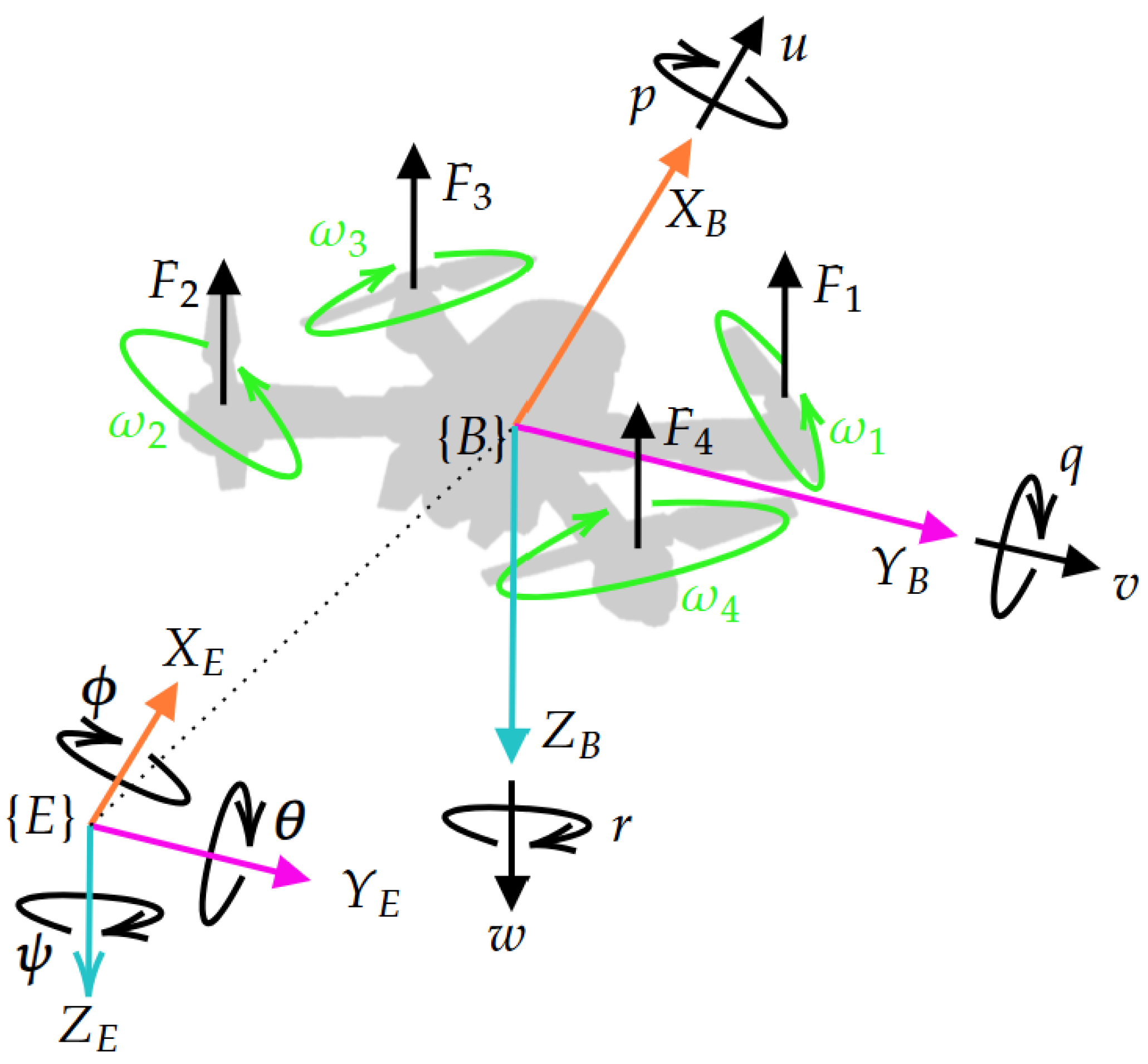
The relative distances between each follower and the leader UAV, as illustrated in in Figure 2, are decomposed into components in the x, y, and z directions. Using the rotation matrix $R\left(\eta \right)$, parameterized by the Euler angles $\varphi$ (roll), $\theta$ (pitch), and $\psi$ (yaw), these distances are formulated as:

$$\left[\begin{array}{c}{L}_{ix}\\ L_{iy}\\ L_{iz}\end{array}\right]=R{\left(\eta \right)}^{-1}\left[\begin{array}{c}{x}_L-x_{Fi}\\ y_L-y_{Fi}\\ z_L-z_{Fi}\end{array}\right],i=1,2,\dots ,n$$

(5)

where $L_{ix}$, $L_{iy}$, and $L_{iz}$ represent the relative distances of the i-th follower UAV in the x, y, and z directions, respectively.

Remark 2. 

The index $i=1,2,\dots ,n$ denotes the number of follower UAVs in the formation, where n is the total number of followers. This formulation is designed to be applicable for any arbitrary number of UAVs because the relative distance equations are defined in a generalized manner, ensuring the scalability of the system. The control strategy does not depend on a fixed number of agents but rather on the ability to compute and regulate each follower’s relative position with respect to the leader. Such generalization is crucial for flexible multi-agent formations, enabling the framework to be applied to various applications, including swarm robotics, cooperative aerial missions, and distributed sensing.

The explicit expressions for the relative distances are given as:

$$\begin{array}{ll}{L}_{ix}& =c_{{\psi }_L}{c}_{{\theta }_L}(x_L-x_{Fi})+s_{{\psi }_L}{c}_{{\theta }_L}(y_L-y_{Fi})-s_{{\theta }_L}(z_L-z_{Fi}),\end{array}$$

(6)

$$\begin{array}{ll}{L}_{iy}& =(c_{{\psi }_L}{s}_{{\theta }_L}{s}_{{\varphi }_L}-s_{{\psi }_L}{c}_{{\varphi }_L})(x_L-x_{Fi})+(s_{{\psi }_L}{s}_{{\theta }_L}{s}_{{\varphi }_L}+c_{{\psi }_L}{c}_{{\varphi }_L})(y_L-y_{Fi})+c_{{\theta }_L}{s}_{{\varphi }_L}(z_L-z_{Fi}),\end{array}$$

(7)

$$\begin{array}{ll}{L}_{iz}& =(c_{{\psi }_L}{s}_{{\theta }_L}{c}_{{\varphi }_L}+s_{{\psi }_L}{s}_{{\varphi }_L})(x_L-x_{Fi})+(s_{{\psi }_L}{s}_{{\theta }_L}{c}_{{\varphi }_L}-c_{{\psi }_L}{s}_{{\varphi }_L})(y_L-y_{Fi})+c_{{\theta }_L}{c}_{{\varphi }_L}(z_L-z_{Fi}).\end{array}$$

(8)

To express the time evolution of the relative distances, we introduce the angular error terms defined as ${ϵ}_{\psi }={\psi }_L-{\psi }_F$, ${ϵ}_{\theta }={\theta }_L-{\theta }_F$, and ${ϵ}_{\varphi }={\varphi }_L-{\varphi }_F$. These errors quantify the difference between the leader and follower UAV orientations. Using trigonometric identities, the derivatives of the relative distances are computed as:

$${\dot{L}}_{ix}={\dot{L}}_y{\dot{\psi }}_L-{\dot{x}}_L+{\dot{x}}_F{c}_{{ϵ}_{\theta }}+{\dot{y}}_F{s}_{{ϵ}_{\theta }}$$

(9)

$${\dot{L}}_{iy}={\dot{x}}_L{s}_{{ϵ}_{\varphi }}+{\dot{x}}_F{c}_{{ϵ}_{\varphi }}-{\dot{y}}_L+{\dot{y}}_F-{\dot{z}}_F{s}_{{ϵ}_{\theta }}$$

(10)

$${\dot{L}}_{iz}={\dot{z}}_L-{\dot{x}}_L{c}_{{ϵ}_{\varphi }}-{\dot{y}}_L{s}_{{ϵ}_{\varphi }}+{\dot{z}}_F{c}_{{ϵ}_{\theta }}$$

(11)

where ${\dot{x}}_L,{\dot{y}}_L,{\dot{z}}_L$ are the leader’s linear velocities in the x, y, and z directions, and ${\dot{x}}_{Fi},{\dot{y}}_{Fi},{\dot{z}}_{Fi}$ are the corresponding velocities of the i-th follower UAV.

Error Dynamics and Control Design

Our control approach is divided into two main parts: position control and attitude control. The position controller is responsible for managing the relative distances in the x, y, and z directions to maintain the UAV formation within a three-dimensional space, even in the presence of external disturbances.

Remark 3. 

Without loss of generality, we consider the relative distances between the leader and a single follower. These formulations can be applied to any follower within the formation, ensuring a consistent approach to maintaining the desired configuration. From this point forward, $L_{xi}$, $L_{yi}$, and $L_{zi}$ will be denoted as $L_x$, $L_y$, and $L_z$, respectively. Similarly, $x_{Fi}$, $y_{Fi}$, and $z_{Fi}$ will be referred to as $x_F$, $y_F$, and $z_F$, and the follower’s velocities ${\dot{x}}_{Fi}$, ${\dot{y}}_{Fi}$, and $w_{Fi}$ will be written as ${\dot{x}}_F$, ${\dot{y}}_F$, and $w_F$.

The position errors are defined as the differences between the actual relative distances and their desired values. Specifically, the errors are calculated as follows:

$$e_x=L_x-L_{x,d},$$

(12)

$$e_y=L_y-L_{y,d},$$

(13)

$$e_z=L_z-L_{z,d}.$$

(14)

where $L_{x,d}$, $L_{y,d}$, and $L_{z,d}$ are the desired distances between the follower and the leader along the x, y, and z axes, respectively. These desired distances are components of the overall desired separation $L_d$, which defines the target spacing between the leader and follower UAVs in three-dimensional space. By minimizing the tracking errors $e_x$, $e_y$, and $e_z$, the control strategy ensures stable and precise formation maintenance while compensating for disturbances.

The dynamics of these errors are given by:

$${\dot{e}}_x={\dot{L}}_x-{\dot{L}}_{x,d},$$

(15)

$${\dot{e}}_y={\dot{L}}_y-{\dot{L}}_{y,d},$$

(16)

$${\dot{e}}_z={\dot{L}}_z-{\dot{L}}_{z,d}.$$

(17)

$$\begin{array}{ll}{\dot{e}}_x=& \left({\dot{L}}_y{\dot{\psi }}_L-{\dot{x}}_L+{\dot{x}}_F{c}_{{ϵ}_{\theta }}+{\dot{y}}_F{s}_{{ϵ}_{\theta }}\right)-{\dot{L}}_{x,d}\end{array}$$

(18)

$$\begin{array}{ll}{\dot{e}}_y=& \left({\dot{x}}_L{s}_{{ϵ}_{\varphi }}+{\dot{x}}_F{c}_{{ϵ}_{\varphi }}-{\dot{y}}_L+{\dot{y}}_F-{\dot{z}}_F{s}_{{ϵ}_{\theta }}\right)-{\dot{L}}_{y,d}\end{array}$$

(19)

$$\begin{array}{ll}{\dot{e}}_z=& \left({\dot{z}}_L-{\dot{x}}_L{c}_{{ϵ}_{\varphi }}-{\dot{y}}_L{s}_{{ϵ}_{\varphi }}+{\dot{z}}_F{c}_{{ϵ}_{\theta }}\right)-{\dot{L}}_{z,d}\end{array}$$

(20)

Assumption 2. 

The desired relative distances $L_{x,d}$, $L_{y,d}$, and $L_{z,d}$, along with their time derivatives ${\dot{L}}_{x,d}$, ${\dot{L}}_{y,d}$, and ${\dot{L}}_{z,d}$, are bounded.

In Assumption 2, the relative distances $L_{x,d},L_{y,d},L_{z,d}$, and their time derivatives ${\dot{L}}_{x,d},{\dot{L}}_{y,d}$ and $L_{z,d}$, are assumed to be bounded. This assumption is fundamental in real-world UAV applications, as it ensures controlled formation and smooth trajectory tracking, while preventing unbounded velocity changes, which would otherwise result in physically infeasible or unsafe maneuvers. In waypoint-based navigation, such bounded values mitigate abrupt changes in relative positioning, enabling smooth and dynamically consistent trajectory transitions. Furthermore, constraining the time derivatives limits velocity fluctuations, preventing excessive accelerations that could destabilize the system or degrade control performance. This requirement is particularly critical in applications such as autonomous surveillance, cooperative UAV operations, and payload transport, where maintaining precise inter-vehicle spacing and ensuring smooth motion transitions are crucial for operational success.

Now considering the following virtual controls:

$$\begin{array}{ll}-k_x{e}_x-k_{0,x}I{e}_x=& \left({\dot{L}}_y{\dot{\psi }}_L-{\dot{x}}_L+{\dot{x}}_{F,d}{c}_{{ϵ}_{\theta }}+{\dot{y}}_F{s}_{{ϵ}_{\theta }}\right)-{\dot{L}}_{x,d}\end{array}$$

(21)

$$\begin{array}{ll}-k_y{e}_y-k_{0,y}I{e}_y=& \left({\dot{x}}_L{s}_{{ϵ}_{\varphi }}+{\dot{x}}_F{c}_{{ϵ}_{\varphi }}-{\dot{y}}_L+{\dot{y}}_{F,d}-{\dot{z}}_F{s}_{{ϵ}_{\theta }}\right)-{\dot{L}}_{y,d}\end{array}$$

(22)

$$\begin{array}{ll}-k_z{e}_z-k_{0,z}I{e}_z=& \left({\dot{z}}_L-{\dot{x}}_L{c}_{{ϵ}_{\varphi }}-{\dot{y}}_L{s}_{{ϵ}_{\varphi }}+{\dot{z}}_{F,d}{c}_{{ϵ}_{\theta }}\right)-{\dot{L}}_{z,d}\end{array}$$

(23)

where $I{e}_j$ is an integrative term defined by ${\dot{Ie}}_j=e_j$, $k_j$ corresponds to the proportional gain, and $k_{0,j}$ is the integral gain, with $j=x,y,z$. In this manner, it is feasible to get ${\dot{x}}_d$, ${\dot{y}}_d$ and ${\dot{z}}_d$ as follows

$${\dot{x}}_d={\dot{x}}_{F,d}={\displaystyle \frac{k_x{e}_x+k_{0,x}I{e}_x+{\dot{L}}_{x,d}-{\dot{L}}_y{\dot{\psi }}_L+{\dot{x}}_L-{\dot{y}}_F{s}_{{ϵ}_{\theta }}}{c_{{ϵ}_{\theta }}}}$$

(24)

$$\begin{array}{l}{\dot{y}}_d={\dot{y}}_{F,d}=k_y{e}_y+k_{0,y}I{e}_y+{\dot{L}}_{y,d}-{\dot{x}}_L{s}_{{ϵ}_{\varphi }}-{\dot{x}}_F{c}_{{ϵ}_{\varphi }}+{\dot{y}}_L+{\dot{z}}_F{s}_{{ϵ}_{\theta }}\end{array}$$

(25)

$${\dot{z}}_d={\dot{z}}_{F,d}={\displaystyle \frac{k_z{e}_z+k_{0,z}I{e}_z+{\dot{L}}_{z,d}-{\dot{z}}_L+{\dot{x}}_L{c}_{{ϵ}_{\varphi }}+{\dot{y}}_L{s}_{{ϵ}_{\varphi }}}{c_{{ϵ}_{\theta }}}}$$

(26)

Now we can define the errors $e_{\dot{x}}=\dot{x}-{\dot{x}}_d$, $e_{\dot{y}}=\dot{y}-{\dot{y}}_d$, and $e_{\dot{z}}=\dot{z}-{\dot{z}}_d$, and upon derivation, we obtain ${\dot{e}}_{\dot{x}}=\ddot{x}-{\ddot{x}}_d$, ${\dot{e}}_{\dot{y}}=\ddot{y}-{\ddot{y}}_d$, and ${\dot{e}}_{\dot{z}}=\ddot{z}-{\ddot{z}}_d$, where the terms ${\ddot{x}}_d$, ${\ddot{y}}_d$, and ${\ddot{z}}_d$ are obtained numerically from (24), (25) and (26), respectively.

Therefore, the dynamics of the tracking error can be expressed as

$${\dot{e}}_{\dot{x}}={\displaystyle \frac{1}{m}}\left(s_{\psi }{s}_{\varphi }+c_{\psi }{s}_{\theta }{c}_{\varphi }\right)U_1+{\displaystyle \frac{F_x}{m}}-{\ddot{x}}_d$$

(27)

$${\dot{e}}_{\dot{y}}={\displaystyle \frac{1}{m}}\left(-c_{\psi }{s}_{\varphi }+s_{\psi }{s}_{\theta }{c}_{\varphi }\right)U_1+{\displaystyle \frac{F_y}{m}}-{\ddot{y}}_d$$

(28)

$${\dot{e}}_{\dot{z}}=-g+{\displaystyle \frac{1}{m}}{c}_{\theta }{c}_{\varphi }{U}_1+{\displaystyle \frac{F_z}{m}}-{\ddot{z}}_d$$

(29)

However, to ensure the robustness of the closed-loop system against parameter variations, external disturbances, and unmodeled dynamics, these effects must be explicitly incorporated into the tracking error dynamics. By rewriting the system equations using nominal parameters and forces, the unknown terms influencing the dynamics become evident, which allows for a more accurate modeling and control of the follower’s response to external influences, thus ensuring the effectiveness of the control strategy under varying conditions. Therefore, denoting $m^{\circ }$ as the nominal mass of the UAV and $F_x^{\circ },F_y^{\circ },F_z^{\circ }$ as the nominal values of the aerodynamic force components in the $x,y,z$ directions, respectively, the dynamic system described in (27)–(29) can be rewritten as follows:

$${\dot{e}}_{\dot{x}}={\displaystyle \frac{1}{m^{\circ }}}\left(s_{\psi }{s}_{\varphi }+c_{\psi }{s}_{\theta }{c}_{\varphi }\right)U_1+{\displaystyle \frac{F_x^{\circ }}{m^{\circ }}}-{\ddot{x}}_d+{\delta }_x$$

(30)

$${\dot{e}}_{\dot{y}}={\displaystyle \frac{1}{m^{\circ }}}\left(-c_{\psi }{s}_{\varphi }+s_{\psi }{s}_{\theta }{c}_{\varphi }\right)U_1+{\displaystyle \frac{F_y^{\circ }}{m^{\circ }}}-{\ddot{y}}_d+{\delta }_y$$

(31)

$${\dot{e}}_{\dot{z}}=-g+{\displaystyle \frac{1}{m^{\circ }}}{c}_{\theta }{c}_{\varphi }{U}_1+{\displaystyle \frac{F_z}{m^{\circ }}}-{\ddot{z}}_d+{\delta }_z$$

(32)

with

$$\begin{array}{l}{\delta }_x=\left({\displaystyle \frac{1}{m}}-{\displaystyle \frac{1}{m^{\circ }}}\right)\left(s_{\psi }{s}_{\varphi }+c_{\psi }{s}_{\theta }{c}_{\varphi }\right)U_1+\left({\displaystyle \frac{F_x}{m}}-{\displaystyle \frac{{F_x}^{\circ }}{m^{\circ }}}\right)\\ {\delta }_y=\left({\displaystyle \frac{1}{m}}-{\displaystyle \frac{1}{m^{\circ }}}\right)\left(s_{\psi }{s}_{\theta }{c}_{\varphi }-c_{\psi }{s}_{\varphi }\right)U_1+\left({\displaystyle \frac{F_y}{m}}-{\displaystyle \frac{{F_y}^{\circ }}{m^{\circ }}}\right)\\ {\delta }_z=\left({\displaystyle \frac{1}{m}}-{\displaystyle \frac{1}{m^{\circ }}}\right)\left(c_{\theta }{c}_{\varphi }\right)U_1+\left({\displaystyle \frac{F_z}{m}}-{\displaystyle \frac{{F_z}^{\circ }}{m^{\circ }}}\right)\end{array}$$

(33)

Remark 4. 

Within the vectors ${\delta }_j$, $j=x,y,z$ are included the parametric variations and the external disturbances that affect the drone.

To achieve stable tracking, the desired pitch angle ${\theta }_d$ and roll angle ${\varphi }_d$ of the follower UAV are adjusted to align the UAV’s velocities with the desired trajectory. The desired pitch and roll angles are then calculated as follows:

$$\begin{array}{ll}{s}_{{\theta }_d}& ={\displaystyle \frac{m}{c_{\varphi }{c}_{\psi }{U}_1}}\left({\ddot{x}}_d-{\delta }_x-{\displaystyle \frac{1}{m}}\left(s_{\varphi }{s}_{\psi }\right)U_1-{\displaystyle \frac{F_x}{m}}-k_{\dot{x}}{e}_{\dot{x}}-k_{0,\dot{x}}I{e}_{\dot{x}}\right)\end{array}$$

(34)

$$\begin{array}{ll}{s}_{{\varphi }_d}& =-{\displaystyle \frac{m}{c_{\psi }{U}_1}}\left({\ddot{y}}_d-{\delta }_y-{\displaystyle \frac{1}{m}}\left(c_{\varphi }{s}_{\theta }{s}_{\psi }\right)U_1-{\displaystyle \frac{F_y}{m}}-k_{\dot{y}}{e}_{\dot{y}}-k_{0,\dot{y}}I{e}_{\dot{y}}\right)\end{array}$$

(35)

In this way, to impose the references, $\theta$ and $\varphi$ are now treated as tracking errors, as depicted below

$$\begin{array}{ll}{e}_{\varphi }& =s_{\varphi }-s_{{\varphi }_d}\end{array}$$

(36)

$$\begin{array}{ll}{e}_{\theta }& =s_{\theta }-s_{{\theta }_d}\end{array}$$

(37)

Here, $s_{{\varphi }_d}$ and $s_{{\theta }_d}$ represent the desired values of the sine of the roll and pitch angles, respectively. Therefore, the corresponding angles are obtained as ${\varphi }_d=arcsin{\varphi }_d$ and ${\theta }_d=arcsin{\theta }_d$.

By differentiating (36) and (37), and applying the chain rule, we obtain the error dynamics, which are given by:

$${\dot{e}}_{\varphi }=c_{\varphi }\dot{\varphi }-{\displaystyle \frac{\mathrm{d}}{\mathrm{dt}}}{s}_{{\varphi }_d}$$

(38)

$${\dot{e}}_{\theta }=c_{\theta }\dot{\theta }-{\displaystyle \frac{\mathrm{d}}{\mathrm{dt}}}{s}_{{\theta }_d}$$

(39)

By the utilization of the virtual controls $-k_{\varphi }{e}_{\varphi }-k_{0,\varphi }I{e}_{\varphi }=c_{\varphi }{\dot{\varphi }}_d-{\displaystyle \frac{\mathrm{d}}{\mathrm{dt}}}{s}_{{\varphi }_d}$ for (36) and $-k_{\theta }{e}_{\theta }-k_{0,\theta }I{e}_{\theta }=c_{\theta }{\dot{\theta }}_d-{\displaystyle \frac{\mathrm{d}}{\mathrm{dt}}}{s}_{{\theta }_d}$ for (37), where $I{e}_k$ is an integrative term defined by ${\dot{Ie}}_k=e_k$, $k_{k_1}$ corresponds to the proportional gain, and $k_{0,k_1}$ is the integral gain with $k=\varphi ,\theta$, it is feasible to get ${\dot{\varphi }}_d$ and ${\dot{\theta }}_d$ as follows

$${\dot{\varphi }}_d={\displaystyle \frac{1}{c_{\varphi }}}\left({\displaystyle \frac{\mathrm{d}}{\mathrm{dt}}}{s}_{{\varphi }_d}-k_{\varphi }{e}_{\varphi }-k_{0,\varphi }I{e}_{\varphi }\right)$$

(40)

$${\dot{\theta }}_d={\displaystyle \frac{1}{c_{\theta }}}\left({\displaystyle \frac{\mathrm{d}}{\mathrm{dt}}}{s}_{{\theta }_d}-k_{\theta }{e}_{\theta }-k_{0,\theta }I{e}_{\theta }\right)$$

(41)

Now, by defining the tracking errors $e_{\dot{\varphi }}=\dot{\varphi }-{\dot{\varphi }}_d$, $e_{\dot{\theta }}=\dot{\theta }-{\dot{\theta }}_d$ along with their corresponding derivatives ${\dot{e}}_{\dot{\varphi }}=\ddot{\varphi }-{\ddot{\varphi }}_d$ and ${\dot{e}}_{\dot{\theta }}=\ddot{\theta }-{\ddot{\theta }}_d$, the error dynamics are obtained

$${\dot{e}}_{\dot{\varphi }}=\left({\displaystyle \frac{I_{yy}-I_{zz}}{I_{xx}}}\right)\dot{\theta }\dot{\psi }-{\displaystyle \frac{I_r}{I_{xx}}}\dot{\theta }{\Omega }_r+{\displaystyle \frac{l}{I_{xx}}}{U}_2+{\displaystyle \frac{T_{\varphi }}{I_{xx}}}-{\ddot{\varphi }}_d$$

(42)

$${\dot{e}}_{\dot{\theta }}=\left({\displaystyle \frac{I_{zz}-I_{xx}}{I_{yy}}}\right)\dot{\varphi }\dot{\psi }+{\displaystyle \frac{I_r}{I_{yy}}}p{\Omega }_r+{\displaystyle \frac{l}{I_{yy}}}{U}_3+{\displaystyle \frac{T_{\theta }}{I_{yy}}}-{\ddot{\theta }}_d$$

(43)

Unlike the pitch and roll angles, the reference for the yaw angle is not derived from a virtual control law but is directly given by the leader UAV’s orientation. Therefore, the tracking error is defined as $e_{\psi }=\psi -{\psi }_L$, where ${\psi }_L$ denotes the leader’s yaw angle. The time derivative of this error is ${\dot{e}}_{\psi }=\dot{\psi }-{\dot{\psi }}_L$. To stabilize this error, a virtual control is defined as $-k_{\psi }{e}_{\psi }-k_{0,\psi }I{e}_{\psi }={\dot{\psi }}_d-{\dot{\psi }}_L$, where $I{e}_{\psi }$ is an integral term defined by ${\dot{Ie}}_{\psi }=e_{\psi }$. This formulation allows for the computation of the desired angular velocity ${\dot{\psi }}_d$, which is used in the error dynamics defined below:

$${\dot{e}}_{\dot{\psi }}=\left({\displaystyle \frac{I_{xx}-I_{yy}}{I_{zz}}}\right)\dot{\varphi }\dot{\theta }+{\displaystyle \frac{U_4}{I_{zz}}}+{\displaystyle \frac{T_{\psi }}{I_{zz}}}-{\ddot{\psi }}_d+{\delta }_{\psi }$$

(44)

To ensure the robustness of the closed-loop system against parameter variations, external disturbances, and unmodeled dynamics, these effects must be explicitly incorporated into the tracking error dynamics. Accordingly, following the approach used in Equations (30)–(32) and considering the perturbations affecting the drone, Equations (42)–(44) can be reformulated as follows.

$${\dot{e}}_{\dot{\varphi }}=\left({\displaystyle \frac{I_{yy}^{\circ }-I_{zz}^{\circ }}{I_{xx}^{\circ }}}\right)\dot{\theta }\dot{\psi }-{\displaystyle \frac{I_r^{\circ }}{I_{xx}^{\circ }}}\dot{\theta }{\Omega }_r+{\displaystyle \frac{l}{I_{xx}^{\circ }}}{U}_2+{\displaystyle \frac{T_{\varphi }}{I_{xx}^{\circ }}}-{\ddot{\varphi }}_d$$

(45)

$${\dot{e}}_{\dot{\theta }}=\left({\displaystyle \frac{I_{zz}^{\circ }-I_{xx}^{\circ }}{I_{yy}^{\circ }}}\right)\dot{\varphi }\dot{\psi }+{\displaystyle \frac{I_r^{\circ }}{I_{yy}^{\circ }}}p{\Omega }_r+{\displaystyle \frac{l}{I_{yy}^{\circ }}}{U}_3+{\displaystyle \frac{T_{\theta }}{I_{yy}^{\circ }}}-{\ddot{\theta }}_d+{\delta }_{\theta }$$

(46)

$${\dot{e}}_{\dot{\psi }}=\left({\displaystyle \frac{I_{xx}^{\circ }-I_{yy}^{\circ }}{I_{zz}^{\circ }}}\right)\dot{\psi }\dot{\theta }+{\displaystyle \frac{U_4}{I_{zz}^{\circ }}}+{\displaystyle \frac{T_{\psi }}{I_{zz}^{\circ }}}-{\ddot{\psi }}_d+{\delta }_{\psi }$$

(47)

where $I_{xx}^{\circ },I_{yy}^{\circ },I_{zz}^{\circ }$ are the nominal value of the inertia terms and $I_r^{\circ }$ is the nominal value of the rotor inertia and

$$\begin{array}{ll}{\delta }_{\varphi }& =\left({\displaystyle \frac{I_{yy}-I_{zz}}{I_{xx}}}-{\displaystyle \frac{{I_{yy}}^{\circ }-{I_{zz}}^{\circ }}{{I_{xx}}^{\circ }}}\right)\dot{\theta }\dot{\psi }-\left({\displaystyle \frac{I_r}{I_{xx}}}-{\displaystyle \frac{{I_r}^{\circ }}{{I_{xx}}^{\circ }}}\right)\dot{\theta }{\Omega }_r\\ & +\left({\displaystyle \frac{l}{I_{xx}}}-{\displaystyle \frac{l}{{I_{xx}}^{\circ }}}\right)U_2+\left({\displaystyle \frac{T_{\varphi }}{I_{xx}}}-{\displaystyle \frac{{T_{\varphi }}^{\circ }}{{I_{xx}}^{\circ }}}\right)\\ {\delta }_{\theta }& =\left({\displaystyle \frac{I_{zz}-I_{xx}}{I_{yy}}}-{\displaystyle \frac{{I_{zz}}^{\circ }-{I_{xx}}^{\circ }}{{I_{yy}}^{\circ }}}\right)\dot{\varphi }\dot{\psi }+\left({\displaystyle \frac{I_r}{I_{yy}}}-{\displaystyle \frac{{I_r}^{\circ }}{{I_{yy}}^{\circ }}}\right)\dot{\varphi }{\Omega }_r\\ & +\left({\displaystyle \frac{l}{I_{yy}}}-{\displaystyle \frac{l}{{I_{yy}}^{\circ }}}\right)U_3+\left({\displaystyle \frac{T_{\theta }}{I_{yy}}}-{\displaystyle \frac{{T_{\theta }}^{\circ }}{{I_{yy}}^{\circ }}}\right)\\ {\delta }_{\psi }& =\left({\displaystyle \frac{I_{xx}-I_{yy}}{I_{zz}}}-{\displaystyle \frac{{I_{xx}}^{\circ }-{I_{yy}}^{\circ }}{{I_{zz}}^{\circ }}}\right)\dot{\varphi }\dot{\theta }+\left({\displaystyle \frac{1}{I_{zz}}}-{\displaystyle \frac{1}{{I_{zz}}^{\circ }}}\right)U_4\\ & +\left({\displaystyle \frac{T_{\psi }}{I_{zz}}}-{\displaystyle \frac{{T_{\psi }}^{\circ }}{{I_{zz}}^{\circ }}}\right)\end{array}$$

(48)

Remark 5. 

Within the vectors ${\delta }_k$, $k=\varphi ,\theta ,\psi$ are included the parametric variations and the external disturbances that affect the drone.

4. Design of Robust Control of UAV Formation Under Parametric Variations and External Disturbances

To achieve robustness of the system (9)–(11) with respect to parametric uncertainties and external disturbance, an HOSM estimator will be used for the estimation of the unknown external disturbances ${\delta }_x,{\delta }_y,{\delta }_z,{\delta }_{\varphi },{\delta }_{\theta },{\delta }_{\psi }$. The HOSM estimator provides a finite-time estimate of parametric uncertainties and external perturbations, assuming their derivatives are bounded. It has been demonstrated [48] that this estimator ensures robust performance under these conditions. The HOSM estimator employs the operators ${\lfloor ·\rceil }^{1/2}={|·|}^{1/2}\mathrm{sign}(·)$ and ${\lfloor ·\rceil }^0=\mathrm{sign}(·)$

The HOSM estimators are defined as follows:

$$\begin{array}{ll}{\dot{\xi }}_x& =-{\lambda }_x{\lfloor {\xi }_x-e_x\rceil }^{1/2}+{\xi }_{\dot{x}}+{\displaystyle \frac{1}{m^{\circ }}}\left(s_{\psi }{s}_{\varphi }+c_{\psi }{s}_{\theta }{c}_{\varphi }\right)U_1+{\displaystyle \frac{{F_x}^{\circ }}{m^{\circ }}}-{\ddot{x}}_d\\ {\dot{\xi }}_{\dot{x}}& =-{\lambda }_{\dot{x}}{\lfloor {\xi }_x-e_x\rceil }^0\\ {\dot{\xi }}_y& =-{\lambda }_y{\lfloor {\xi }_y-e_y\rceil }^{1/2}+{\xi }_{\dot{y}}+{\displaystyle \frac{1}{m^{\circ }}}\left(s_{\psi }{s}_{\theta }co{s}_{\varphi }-c_{\psi }{s}_{\varphi }\right)U_1+{\displaystyle \frac{{F_y}^{\circ }}{m^{\circ }}}-{\ddot{y}}_d\\ {\dot{\xi }}_{\dot{y}}& =-{\lambda }_{\dot{y}}{\lfloor {\xi }_y-e_y\rceil }^0\\ {\dot{\xi }}_z& =-{\lambda }_z{\lfloor {\xi }_z-e_z\rceil }^{1/2}+{\xi }_{\dot{z}}+{\displaystyle \frac{1}{m^{\circ }}}\left(c_{\theta }{c}_{\varphi }\right)U_1+{\displaystyle \frac{{F_z}^{\circ }}{m^{\circ }}}-g-{\ddot{z}}_d\\ {\dot{\xi }}_{\dot{z}}& =-{\lambda }_{\dot{z}}{\lfloor {\xi }_z-e_z\rceil }^0\end{array}$$

(49)

$$\begin{array}{ll}{\dot{\xi }}_{\varphi }& =-{\lambda }_{\varphi }{\lfloor {\xi }_{\varphi }-e_{\varphi }\rceil }^{1/2}+{\xi }_{\dot{\varphi }}+\left({\displaystyle \frac{{I_{yy}}^{\circ }-{I_{zz}}^{\circ }}{{I_{xx}}^{\circ }}}\right)\dot{\theta }\dot{\psi }-\left({\displaystyle \frac{{I_r}^{\circ }}{{I_{xx}}^{\circ }}}\right)\dot{\theta }{\Omega }_r+{\displaystyle \frac{l^{\circ }}{{I_{xx}}^{\circ }}}{U}_2+{\displaystyle \frac{{T_{\varphi }}^{\circ }}{{I_{xx}}^{\circ }}}-{\ddot{\varphi }}_d\\ {\dot{\xi }}_{\dot{\varphi }}& =-{\lambda }_{\dot{\varphi }}{\lfloor {\xi }_{\varphi }-e_{\varphi }\rceil }^0\\ {\dot{\xi }}_{\theta }& =-{\lambda }_{\theta }{\lfloor {\xi }_{\theta }-e_{\theta }\rceil }^{1/2}+{\xi }_{\dot{\theta }}+\left({\displaystyle \frac{{I_{zz}}^{\circ }-{I_{xx}}^{\circ }}{{I_{yy}}^{\circ }}}\right)\dot{\varphi }\dot{\psi }+\left({\displaystyle \frac{{I_r}^{\circ }}{{I_{yy}}^{\circ }}}\right)\dot{\varphi }{\Omega }_r+{\displaystyle \frac{l^{\circ }}{{I_{yy}}^{\circ }}}{U}_3+{\displaystyle \frac{{T_{\theta }}^{\circ }}{{I_{yy}}^{\circ }}}-{\ddot{\theta }}_d\\ {\dot{\xi }}_{\dot{\theta }}& =-{\lambda }_{\dot{\theta }}{\lfloor {\xi }_{\theta }-e_{\theta }\rceil }^0\\ {\dot{\xi }}_{\psi }& =-{\lambda }_{\psi }{\lfloor {\xi }_{\psi }-e_{\psi }\rceil }^{1/2}+{\xi }_{\dot{\psi }}+\left({\displaystyle \frac{{I_{xx}}^{\circ }-{I_{yy}}^{\circ }}{{I_{zz}}^{\circ }}}\right)\dot{\varphi }\dot{\theta }+{\displaystyle \frac{1}{{I_{zz}}^{\circ }}}{U}_4+{\displaystyle \frac{{T_{\psi }}^{\circ }}{{I_{zz}}^{\circ }}}-{\ddot{\psi }}_d\\ {\dot{\xi }}_{\dot{\psi }}& =-{\lambda }_{\dot{\psi }}{\lfloor {\xi }_{\psi }-e_{\psi }\rceil }^0\end{array}$$

(50)

Using the HOSM estimators (49) and (50) and to ensure that the estimation errors $E_{\dot{x}}={\xi }_{\dot{x}}-{\delta }_x$, $E_{\dot{y}}={\xi }_{\dot{y}}-{\delta }_y$, $E_{\dot{z}}={\xi }_{\dot{z}}-{\delta }_z$, $E_{\dot{\varphi }}={\xi }_{\dot{\varphi }}-{\delta }_{\varphi }$, $E_{\dot{\theta }}={\xi }_{\dot{\theta }}-{\delta }_{\theta }$, and $E_{\dot{\psi }}={\xi }_{\dot{\psi }}-{\delta }_{\psi }$ converge to zero in finite time, the following conditions must be satisfied

$$\begin{array}{ll}{\lambda }_{j,1}& >0,{\lambda }_{j,2}>3{\Delta }_{j,max}+2{\Delta }_{j,max}^2/{\lambda }_{j,1}^2\\ {\lambda }_{k,1}& >0,{\lambda }_{k,2}>3{\Delta }_{k,max}+2{\Delta }_{k,max}^2/{\lambda }_{k,1}^2\\ k_{j_2}& >0,k_{0,j_2}>0,k_{k_2}>0,k_{0,k_2}>0\end{array}$$

(51)

for $j=x,y,z$ and $k=\varphi ,\theta ,\psi$, ensuring that ${\Delta }_{j,max},{\Delta }_{k,max}\in \mathbb{R}$ remain bounded within appropriate limits.

The dynamics of the estimation errors $E_{\dot{x}}={\xi }_{\dot{x}}-{\delta }_x$, $E_{\dot{y}}={\xi }_{\dot{y}}-{\delta }_y$, $E_{\dot{z}}={\xi }_{\dot{z}}-{\delta }_z$, $E_{\dot{\varphi }}={\xi }_{\dot{\varphi }}-{\delta }_{\varphi }$, $E_{\dot{\theta }}={\xi }_{\dot{\theta }}-{\delta }_{\theta }$, and $E_{\dot{\psi }}={\xi }_{\dot{\psi }}-{\delta }_{\psi }$ using the HOSM estimators (49) and (50) along with the tracking errors (30), (31), (32), (45), (46) and (47) can be rewritten as

$$\begin{array}{ll}{\dot{e}}_x& =-{\lambda }_x{\lfloor e_x\rceil }^{1/2}+e_{\dot{x}}\\ {\dot{e}}_{\dot{x}}& =-{\lambda }_{\dot{x}}{\lfloor e_x\rceil }^0-{\dot{\delta }}_x\\ {\dot{e}}_y& =-{\lambda }_y{\lfloor e_y\rceil }^{1/2}+e_{\dot{y}}\\ {\dot{e}}_{\dot{y}}& =-{\lambda }_{\dot{y}}{\lfloor e_y\rceil }^0-{\dot{\delta }}_y\\ {\dot{e}}_z& =-{\lambda }_z{\lfloor e_z\rceil }^{1/2}+e_{\dot{z}}\\ {\dot{e}}_{\dot{z}}& =-{\lambda }_{\dot{z}}{\lfloor e_z\rceil }^0-{\dot{\delta }}_z\\ {\dot{e}}_{\varphi }& =-{\lambda }_{\varphi }{\lfloor e_{\varphi }\rceil }^{1/2}+e_{\dot{\varphi }}\\ {\dot{e}}_{\dot{\varphi }}& =-{\lambda }_{\dot{\varphi }}{\lfloor e_{\varphi }\rceil }^0-{\dot{\delta }}_{\varphi }\\ {\dot{e}}_{\theta }& =-{\lambda }_{\theta }{\lfloor e_{\theta }\rceil }^{1/2}+e_{\dot{\theta }}\\ {\dot{e}}_{\dot{\theta }}& =-{\lambda }_{\dot{\theta }}{\lfloor e_{\theta }\rceil }^0-{\dot{\delta }}_{\theta }\\ {\dot{e}}_{\psi }& =-{\lambda }_{\psi }{\lfloor e_{\psi }\rceil }^{1/2}+e_{\dot{\psi }}\\ {\dot{e}}_{\dot{\psi }}& =-{\lambda }_{\dot{\psi }}{\lfloor e_{\psi }\rceil }^0-{\dot{\delta }}_{\psi }\end{array}$$

(52)

These are six decoupled subsystems. Now, considering the subsystem decoupled subsystem

$$\begin{array}{ll}{\dot{e}}_x& =-{\lambda }_x{\lfloor e_x\rceil }^{1/2}+e_{\dot{x}}\\ {\dot{e}}_{\dot{x}}& =-{\lambda }_{\dot{x}}{\lfloor e_x\rceil }^0-{\dot{\delta }}_x\end{array}$$

(53)

we evaluate its stability by defining the Lyapunov candidate function as:

$$\begin{array}{ll}{V}_x& ={\displaystyle \frac{1}{2}}{E}_x^T{P}_x{E}_x\end{array}$$

where

$$P_x=\left(\begin{array}{cc}{\lambda }_x^2+4{\lambda }_{\dot{x}}& -{\lambda }_x\\ -{\lambda }_x& 2\end{array}\right)=P_x^T>0,E_x=\left(\begin{array}{c}{\lfloor e_x\rceil }^{1/2}\\ e_{\dot{x}}\end{array}\right)$$

The time derivative of $E_x$ becomes

$$\begin{array}{ll}{\dot{E}}_x& =-{\displaystyle \frac{1}{2|e_x{|}^{1/2}}}{\lambda }_x{E}_z-{\displaystyle \frac{{\dot{\delta }}_x}{2|e_x{|}^{1/2}}}{\lfloor e_x\rceil }^0{\lambda }_{x_0}{E}_x,\end{array}$$

where

$${\lambda }_x=\left(\begin{array}{cc}{\lambda }_x& -1\\ 2{\lambda }_{\dot{x}}& 0\end{array}\right);{\lambda }_{x_0}=\left(\begin{array}{cc}0& 0\\ 2& 0\end{array}\right)$$

Therefore, the Lyapunov derivative is

$${\dot{V}}_x=-{\displaystyle \frac{{\lambda }_x}{2|e_x{|}^{1/2}}}{E}_x^T{Q}_x{E}_x-{\displaystyle \frac{{\dot{\delta }}_x}{2|e_x{|}^{1/2}}}{\lfloor e_x\rceil }^0{E}_x^T{Q}_{x_0}{E}_x$$

with

$$Q_x={\displaystyle \frac{P_1{\lambda }_x+{\lambda }_{x_0}^T{P}_x}{2{\lambda }_x}}=\left(\begin{array}{cc}{\lambda }_x^2+2{\lambda }_{\dot{x}}& -{\lambda }_x\\ -{\lambda }_x& 1\end{array}\right)$$

$$Q_{x_0}=P_x{\lambda }_{x_0}=\left(\begin{array}{cc}-2{\lambda }_x& 2\\ 2& 0\end{array}\right)$$

Since the derivatives of the external perturbations are assumed to be bounded, it follows that ${\dot{\delta }}_x$ is also bounded over any finite time interval. Let ${\Delta }_{x,max}$ be a positive constant such that $|{\dot{\delta }}_x|\le {\Delta }_{x,max}$. This bound allows us to estimate ${\dot{V}}_x$ as follows:

$$\begin{array}{ll}{\dot{V}}_x& =-{\displaystyle \frac{{\lambda }_x}{2|e_x{|}^{1/2}}}{E}_x^T{Q}_x{E}_x-{\displaystyle \frac{{\dot{\delta }}_x}{2|e_x{|}^{1/2}}}{\lfloor e_x\rceil }^0{E}_x^T{Q}_{x_0}{E}_x\\ & -{\displaystyle \frac{{\lambda }_x}{2|e_x{|}^{1/2}}}{\mathcal{E}}_x^T{Q}_{x{\mathcal{E}}_x}-{\displaystyle \frac{{\Delta }_{x,max}}{2|e_x{|}^{1/2}}}{\mathcal{E}}_x^T{Q}_{x_0}{\mathcal{E}}_x\\ & =-{\displaystyle \frac{{\lambda }_x}{2|e_x{|}^{1/2}}}{\mathcal{E}}_x^T{Q}_x{\mathcal{E}}_x\\ & \le -{\displaystyle \frac{{\lambda }_x}{2|e_x{|}^{1/2}}}{\lambda }_{min}^{Q_x}{\parallel E_x\parallel }_2^2\le -{\gamma }_x{V}_x^{1/2}\end{array}$$

where

$$\begin{array}{l}{\gamma }_x={\lambda }_x{\displaystyle \frac{\sqrt{{\lambda }_{min}^{P_x}}}{\sqrt{2}{\lambda }_{max}^{P_x}}}{\lambda }_{min}^{Q_x}\\ {\mathcal{E}}_x=\left(\begin{array}{c}\phantom{(}|{\lfloor e_x\rceil }^{1/2}|\\ |e_{\dot{x}}|\end{array}\right)\\ Q_x=\left(\begin{array}{cc}{\lambda }_x^2+2{\lambda }_{\dot{x}}-2{\Delta }_{x,\max }& -{\lambda }_x+\frac{2{\Delta }_{x,\max }}{{\lambda }_x}\\ -{\lambda }_x+\frac{2{\Delta }_{x,\max }}{{\lambda }_x}& 1\end{array}\right)\end{array}$$

with ${\lambda }_x>0,{\lambda }_{\dot{x}}>0,Q_x>0,$ and ${\left|\right|{\mathcal{E}}_x\left|\right|}_2^2={\left|\right|E_x\left|\right|}_2^2={\left|{\lfloor e_x\rceil }^{1/2}\right|}^2+{\left|e_{\dot{x}}\right|}^2=\left|e_x\right|+e_{\dot{x}}^2$ Therefore, due to the boundedness of the signals over any finite time interval and the inequality ${\dot{V}}_x\le -{\gamma }_x{V}_x^{1/2}$, we conclude that E_x converges to the origin in finite time.

Similarly, the stability of the remaining subsystems in (52) can be analyzed using the following Lyapunov candidate functions:

$$\begin{array}{l}{V}_y={\displaystyle \frac{1}{2}}{E}_y^T{P}_y{E}_y,\\ P_y=\left(\begin{array}{cc}{\lambda }_y^2+4{\lambda }_{\dot{y}}& -{\lambda }_y\\ -{\lambda }_y& 2\end{array}\right)=P_y^T>0,E_y=\left(\begin{array}{c}{\lfloor e_y\rceil }^{1/2}\\ e_{\dot{y}}\end{array}\right)\\ V_z={\displaystyle \frac{1}{2}}{E}_z^T{P}_z{E}_z,\\ P_z=\left(\begin{array}{cc}{\lambda }_z^2+4{\lambda }_{\dot{z}}& -{\lambda }_z\\ -{\lambda }_z& 2\end{array}\right)=P_z^T>0,E_z=\left(\begin{array}{c}{\lfloor e_z\rceil }^{1/2}\\ e_{\dot{z}}\end{array}\right)\\ V_{\varphi }={\displaystyle \frac{1}{2}}{E}_{\varphi }^T{P}_{\varphi }{E}_{\varphi },\\ P_{\varphi }=\left(\begin{array}{cc}{\lambda }_{\varphi }^2+4{\lambda }_{\dot{\varphi }}& -{\lambda }_{\varphi }\\ -{\lambda }_{\varphi }& 2\end{array}\right)=P_{\varphi }^T>0,E_{\varphi }=\left(\begin{array}{c}{\lfloor e_{\varphi }\rceil }^{1/2}\\ e_{\dot{\varphi }}\end{array}\right)\\ V_{\theta }={\displaystyle \frac{1}{2}}{E}_{\theta }^T{P}_{\theta }{E}_{\theta },\\ P_{\theta }=\left(\begin{array}{cc}{\lambda }_{\theta }^2+4{\lambda }_{\dot{\theta }}& -{\lambda }_{\theta }\\ -{\lambda }_{\theta }& 2\end{array}\right)=P_{\theta }^T>0,E_{\theta }=\left(\begin{array}{c}{\lfloor e_{\theta }\rceil }^{1/2}\\ e_{\dot{\theta }}\end{array}\right)\\ V_{\psi }={\displaystyle \frac{1}{2}}{E}_{\psi }^T{P}_{\psi }{E}_{\psi },\\ P_{\psi }=\left(\begin{array}{cc}{\lambda }_{\psi }^2+4{\lambda }_{\dot{\psi }}& -{\lambda }_{\psi }\\ -{\lambda }_{\psi }& 2\end{array}\right)=P_{\psi }^T>0,E_{\psi }=\left(\begin{array}{c}{\lfloor e_{\psi }\rceil }^{1/2}\\ e_{\dot{\psi }}\end{array}\right)\end{array}$$

where ${\Delta }_{x,\max }$, ${\Delta }_{y,\max }$, ${\Delta }_{\varphi ,\max }$, ${\Delta }_{\theta ,\max }$ and ${\Delta }_{\psi ,\max }$ represent the upper bounds on the derivatives of the disturbance ${\dot{\delta }}_x$, ${\dot{\delta }}_y$, ${\dot{\delta }}_z$, ${\dot{\delta }}_{\varphi }$, ${\dot{\delta }}_{\theta }$ and ${\dot{\delta }}_{\psi }$, respectively, over any finite time interval.

Now, considering the dynamics of the tracking errors (32), (45), (46) and (47), the proposed control inputs are as follows:

$$\begin{array}{ll}{U}_1& ={\displaystyle \frac{m^{\circ }}{c_{\theta }{c}_{\varphi }}}\left({\ddot{z}}_d+g-{\displaystyle \frac{{F_z}^{\circ }}{m^{\circ }}}-k_{\dot{z}}{e}_{\dot{z}}-k_{0,\dot{z}}{Ie}_{\dot{z}}-{\xi }_{\dot{z}}\right)\\ U_2& ={\displaystyle \frac{{I_{xx}}^{\circ }}{l}}\left({\ddot{\varphi }}_d-{\displaystyle \frac{\dot{\theta }\dot{\psi }({I_{yy}}^{\circ }-{I_{zz}}^{\circ })}{{I_{xx}}^{\circ }}}+{\displaystyle \frac{{I_r}^{\circ }\dot{\theta }{\Omega }_r}{{I_{xx}}^{\circ }}}-{\displaystyle \frac{{T_{\varphi }}^{\circ }}{{I_{xx}}^{\circ }}}-k_{\dot{\varphi }}{e}_{\dot{\varphi }}-k_{0,\dot{\varphi }}{Ie}_{\dot{\varphi }}-{\xi }_{\dot{\varphi }}\right)\\ U_3& ={\displaystyle \frac{{I_{yy}}^{\circ }}{l}}\left({\ddot{\theta }}_d-{\displaystyle \frac{\dot{\varphi }\dot{\psi }({I_{zz}}^{\circ }-{I_{xx}}^{\circ })}{{I_{yy}}^{\circ }}}-{\displaystyle \frac{{I_r}^{\circ }\dot{\varphi }{\Omega }_r}{{I_{yy}}^{\circ }}}-{\displaystyle \frac{{T_{\theta }}^{\circ }}{{I_{yy}}^{\circ }}}-k_{\dot{\theta }}{e}_{\dot{\theta }}-k_{0,\dot{\theta }}{Ie}_{\dot{\theta }}-{\xi }_{\dot{\theta }}\right)\\ U_4& ={I_{zz}}^{\circ }\left({\ddot{\psi }}_d-{\displaystyle \frac{\dot{\varphi }\dot{\theta }({I_{xx}}^{\circ }-{I_{yy}}^{\circ })}{{I_{zz}}^{\circ }}}-{\displaystyle \frac{{T_{\psi }}^{\circ }}{{I_{zz}}^{\circ }}}-k_{\dot{\psi }}{e}_{\dot{\psi }}-k_{0,\dot{\psi }}{Ie}_{\dot{\psi }}-{\xi }_{\dot{\psi }}\right)\end{array}$$

(54)

with

$$\begin{array}{ll}\dot{I}{e}_{\dot{z}}& =e_{\dot{z}}\\ \dot{I}{e}_{\dot{\varphi }}& =e_{\dot{\varphi }}\\ \dot{I}{e}_{\dot{\theta }}& =e_{\dot{\theta }}\\ \dot{I}{e}_{\dot{\psi }}& =e_{\dot{\psi }}\end{array}$$

(55)

where $k_i,k_{0,i}>0$ for $i=\dot{z},\dot{\varphi },\dot{\theta },\dot{\psi }$.

Closed-Loop Stability in UAV

In this subsection, the stability properties of the proposed nonlinear robust control approach are examined. Referring to Section 4, it is established that the estimated states ${\xi }_{\dot{x}},{\xi }_{\dot{y}},{\xi }_{\dot{z}},{\xi }_{\dot{\varphi }},{\xi }_{\dot{\theta }},{\xi }_{\dot{\psi }}$ converge in finite time to their respective unknown external disturbances ${\delta }_x,{\delta }_y,{\delta }_z,{\delta }_{\varphi },{\delta }_{\theta },{\delta }_{\psi }$. To analyze closed-loop behavior, we consider the tracking errors that result from parametric variations and external disturbances. The dynamics of ${\dot{e}}_{\dot{x}}$ are described in (30), while the corresponding control input $U_2$ is defined in (54). Based on these expressions, the resulting closed-loop system can be expressed as:

$$\left(\begin{array}{c}\dot{I}{e}_x\\ {\dot{e}}_x\\ \dot{I}{e}_{\dot{x}}\\ {\dot{e}}_{\dot{x}}\\ \dot{I}{e}_{\theta }\\ {\dot{e}}_{\theta }\dot{I}{e}_{\dot{\theta }}\\ {\dot{e}}_{\dot{\theta }}\end{array}\right)=\left(\begin{array}{cccccccc}0& 1& 0& 0& 0& 0& 0& 0\\ -k_{0,x}& -k_x& 0& 1& 0& 0& 0& 0\\ 0& 0& 0& 1& 0& 0& 0& 0\\ 0& 0& -k_{0,\dot{x}}& -k_{\dot{x}}& 0& {\displaystyle \frac{\cos \varphi \cos \psi U_1}{m}}& 0& 0\\ 0& 0& 0& 0& 0& 1& 0& 0\\ 0& 0& 0& 0& -k_{0,\theta }& -k_{\theta }& 0& \cos \theta \\ 0& 0& 0& 0& 0& 0& 0& 1\\ 0& 0& 0& 0& 0& 0& -k_{0,\dot{\theta }}& -k_{\dot{\theta }}\end{array}\right)\left(\begin{array}{c}I{e}_x\\ {\dot{e}}_x\\ I{e}_{\dot{x}}\\ {\dot{e}}_{\dot{x}}\\ I{e}_{\theta }\\ {\dot{e}}_{\theta }\\ I{e}_{\dot{\theta }}\\ {\dot{e}}_{\dot{\theta }}\end{array}\right)+\left(\begin{array}{c}0\\ 0\\ 0\\ {\xi }_{\dot{x}}-{\delta }_x\\ 0\\ 0\\ 0\\ {\xi }_{\dot{\theta }}-{\delta }_{\theta }\end{array}\right)$$

(56)

which are ISS (Input-to-State Stability) with respect to the terms ${\xi }_{\dot{x}}-{\delta }_x$ and ${\xi }_{\dot{\theta }}-{\delta }_{\theta }$. Analyzing matrix (56), the eigenvalues can be computed using Maple, a symbolic and numeric computing software. The eigenvalues are given by:

$$\begin{array}{ll}{\rho }_x& =-k_x/2\pm \sqrt{k_x^2-4k_{0,x}}/2\\ {\rho }_{\dot{x}}& =-k_{\dot{x}}/2\pm \sqrt{k_{\dot{x}}^2-4k_{0,\dot{x}}}/2\\ {\rho }_{\theta }& =-k_{\theta }/2\pm \sqrt{k_{\theta }^2-4k_{0,\theta }}/2\\ {\rho }_{\dot{\theta }}& =-k_{\dot{\theta }}/2\pm \sqrt{k_{\dot{\theta }}^2-4k_{0,\dot{\theta }}}/2\end{array}$$

(57)

which confirms that all eigenvalues of matrix (56) satisfy $\mathrm{Re}\{{\rho }_x,{\rho }_{\dot{x}},$${\rho }_{\theta },{\rho }_{\dot{\theta }}\}<0$ for any set of positive control gains $k_x>0,k_{\dot{x}}>0,k_{0,x}>0,k_{0,\dot{x}}>0$,$k_{\theta }>0,k_{\dot{\theta }}>0,k_{0,\theta }>0,k_{0,\dot{\theta }}>0$. This implies that the matrix is Hurwitz [49]. Therefore, since the terms ${\xi }_{\dot{x}}-{\delta }_x$ and ${\xi }_{\dot{\theta }}-{\delta }_{\theta }$ tends to zero in finite time, the tracking errors $e_x,e_{\dot{x}},e_{\theta },e_{\dot{\theta }}$ are globally uniformly exponentially stable.

In a similar way, the closed-loop analysis of the subsystem used to control the lateral movement can be performed. The dynamics of ${\dot{e}}_{\dot{y}}$ are described in (31), while the corresponding control input $U_3$ is defined in (54). Based on these expressions, the resulting closed-loop system can be analyzed analogously.

On the other hand, we have

$$\left(\begin{array}{c}\dot{I}{e}_z\\ {\dot{e}}_z\\ \dot{I}{e}_{\dot{z}}\\ {\dot{e}}_{\dot{z}}\end{array}\right)=\left(\begin{array}{cccc}0& 1& 0& 0\\ -k_{0,z}& -k_z& 0& 1\\ 0& 0& 0& 1\\ 0& 0& -k_{0,\dot{z}}& -k_{\dot{z}}\end{array}\right)\left(\begin{array}{c}{Ie}_z\\ e_z\\ {Ie}_{\dot{z}}\\ e_{\dot{z}}\end{array}\right)+\left(\begin{array}{c}0\\ 0\\ 0\\ {\xi }_{\dot{z}}-{\delta }_z\end{array}\right)$$

(58)

which are ISSs with respect to the terms ${\xi }_{\dot{z}}-{\delta }_z$. In this case, the dynamics of ${\dot{e}}_{\dot{z}}$ are derived from (32), and the corresponding control input $U_1$ is defined in (54). By analyzing (58), we can also compute the eigenvalues, which are

$$\begin{array}{ll}{\rho }_z& =-k_z/1\pm \sqrt{k_z^2-4k_{0,z}}/2\\ {\rho }_{\dot{z}}& =-k_{\dot{z}}/2\pm \sqrt{k_{\dot{z}}^2-4k_{0,\dot{z}}}/2\end{array}$$

(59)

These results show that all eigenvalues of matrix (58) satisfy $\mathrm{Re}\{{\rho }_z,{\rho }_{\dot{z}}\}<0$ for any positive values of $k_{0,z}>0,k_z>0,k_{0,\dot{z}}>0,k_{\dot{z}}>0$, i.e., the matrix is Hurwitz [49]. Therefore, since the term ${\xi }_{\dot{z}}-{\delta }_z$ tend to zero in finite time, the tracking errors $e_z,e_{\dot{z}}$ are globally uniformly exponentially stable.

The stability analysis of the subsystem used to control the yaw motion can be performed in a similar manner. The dynamics of ${\dot{e}}_{\dot{\psi }}$ are described in (44), while the corresponding control input $U_4$ is defined in (54). These expressions allow the closed-loop behavior of the yaw subsystem to be examined following the same procedure.

5. Simulation Results

To assess the performance of the proposed robust formation control strategy, simulations were conducted using MATLAB/Simulink with a multi-UAV setup involving one leader and two followers. The objective was to ensure that the followers maintain predefined relative distances with respect to the leader UAV while tracking its trajectory in a three-dimensional space, despite the presence of parametric uncertainties and external disturbances.

To evaluate the robustness of the control strategy, the simulation setup incorporated both external disturbances and parametric variations. Concerning external disturbances, wind disturbances were applied with different velocities for each UAV: the leader experienced a nominal wind speed of 10 m/s, while the followers were subjected to 5 m/s. This configuration emulates realistic scenarios where the UAVs operate under heterogeneous environmental conditions.

Wind dynamics play a crucial role in UAV behavior, especially in outdoor missions where wind patterns are rarely uniform. To capture this, the simulations incorporated lateral wind gusts with time-varying characteristics. The wind velocity at any given moment was defined by its components in the Earth-fixed frame as $v_W={(v_{W,X},v_{W,Y})}^T$, where the components $v_{W,X}$ and $v_{W,Y}$ are calculated using $v_{W,X}=V_w\cos ({\beta }_0+\Delta {\beta }_0)+0.025N$ and $v_{W,Y}=V_{w}sin({\beta }_0+\Delta {\beta }_0)+0.025N$, respectively. Here, $V_w=V_{w,0}+\Delta V_{w}sin\left({\omega }_w\right)$ represents the time-varying wind speed, with $V_{w,0}$ being the nominal wind speed, ${\beta }_0$ the nominal wind direction, and N a uniform random variable simulating small perturbations. The terms $\Delta {\beta }_0=0.2{\beta }_0$ and $\Delta V_w=0.1V_{w,0}$ introduce variations in the wind direction and intensity, ensuring realistic disturbance modeling.

Once the wind velocity was determined in the Earth-fixed frame, it was transformed into the body-fixed frame of the UAVs, where it directly influenced their motion dynamics. This transformation was carried out using the relations $v_{w,x}=v_{W,X}\cos {\alpha }_z+v_{W,Y}sin{\alpha }_z$ and $v_{w,y}=-v_{W,X}sin{\alpha }_z+v_{W,Y}\cos {\alpha }_z$. The apparent wind acting on each UAV was computed by subtracting the vehicle’s own velocity from the wind velocity, leading to the effective wind components $v_{aw,x}=v_x-v_{w,x}$ and $v_{aw,y}=v_y-v_{w,y}$.

These apparent wind components induced aerodynamic forces and moments, primarily affecting longitudinal and lateral motion. The forces generated by the wind were modeled using standard aerodynamic coefficients, where the force in the x-direction is given by $F_x=-{\displaystyle \frac{1}{2}}{A}_x\rho C_d{v}_{aw,x}^2$ and the force in the y-direction is given by $F_y=-{\displaystyle \frac{1}{2}}{A}_y\rho C_d{v}_{aw,y}^2$. Additionally, the wind-induced torques acting on the UAV were given by $T_{\varphi }=-l_{c,z}{F}_y$, $T_{\theta }=-l_{c,z}{F}_x$, and $T_{\psi }=l_{c,x}{F}_y-l_{c,y}{F}_x$.

In these equations, $A_x$ and $A_y$ represent the UAV’s frontal and lateral surface areas, $\rho$ is the air density, $C_d$ is the aerodynamic drag coefficient, and $l_{c,x},l_{c,y}$ are the distances from the center of mass to the aerodynamic center in the respective directions.

The overall effect of wind disturbances on each UAV depended on its orientation, velocity, and position within the formation. Given that the leader UAV was subjected to a higher wind speed compared to the followers, its control system had to exert additional effort to preserve the intended formation geometry. The resulting aerodynamic forces and moments significantly impacted the roll, pitch, and yaw dynamics of each vehicle, requiring an adaptive and robust response from the control strategy to effectively counteract the effects of external perturbations.

For simplicity, only wind components along the x- and y-axes were considered in this study. This assumption allows us to focus on the dominant effects in horizontal plane control, while reducing computational complexity. The exclusion of the z-component simplifies the simulation without significantly affecting the evaluation of the proposed control strategy, which primarily operates in the horizontal motion dynamics. The specific wind conditions applied during the simulations included a nominal wind speed of $V_{w,0}=10$ m/s for the leader and $V_{w,0}=5$ m/s for both followers. Also, it was considered a predominant wind direction of ${\beta }_0={\displaystyle \frac{7\pi }{4}}$ rad, and a wind oscillation frequency of ${\omega }_w=0.1$ rad/s.

On the other hand, to challenge the control framework, parametric variations were also introduced in the UAV dynamics as shown in

Table 1. Parametric variations considered.

Parameter	Nominal Value	Variation
Mass m	1.3 kg	$1.05m$
Thrust Coefficient $C_{\tau }$	0.0048	$1.0C_{\tau }$
Drag Coefficient $C_D$	0.0002351	$1.0C_D$
Inertia $I_{xx},I_{yy},I_{zz}$	(0.081, 0.081, 0.142) kg m2	$1.05I_{xx},1.05I_{yy},1.05I_{zz}$

, which include changes in mass, thrust, and drag coefficients and inertia values. These parametric variations simulate real-world uncertainties in vehicle properties and allow assessment of the controller’s robustness.

The simulation results, depicted in Figure 3, Figure 4, Figure 5, Figure 6, Figure 7, Figure 8 and Figure 9, validate the performance of the proposed robust formation control strategy under parametric uncertainties and external disturbances. The objective was to ensure that two follower UAVs maintain predefined relative distances with respect to a leader UAV while tracking its trajectory in three-dimensional space.

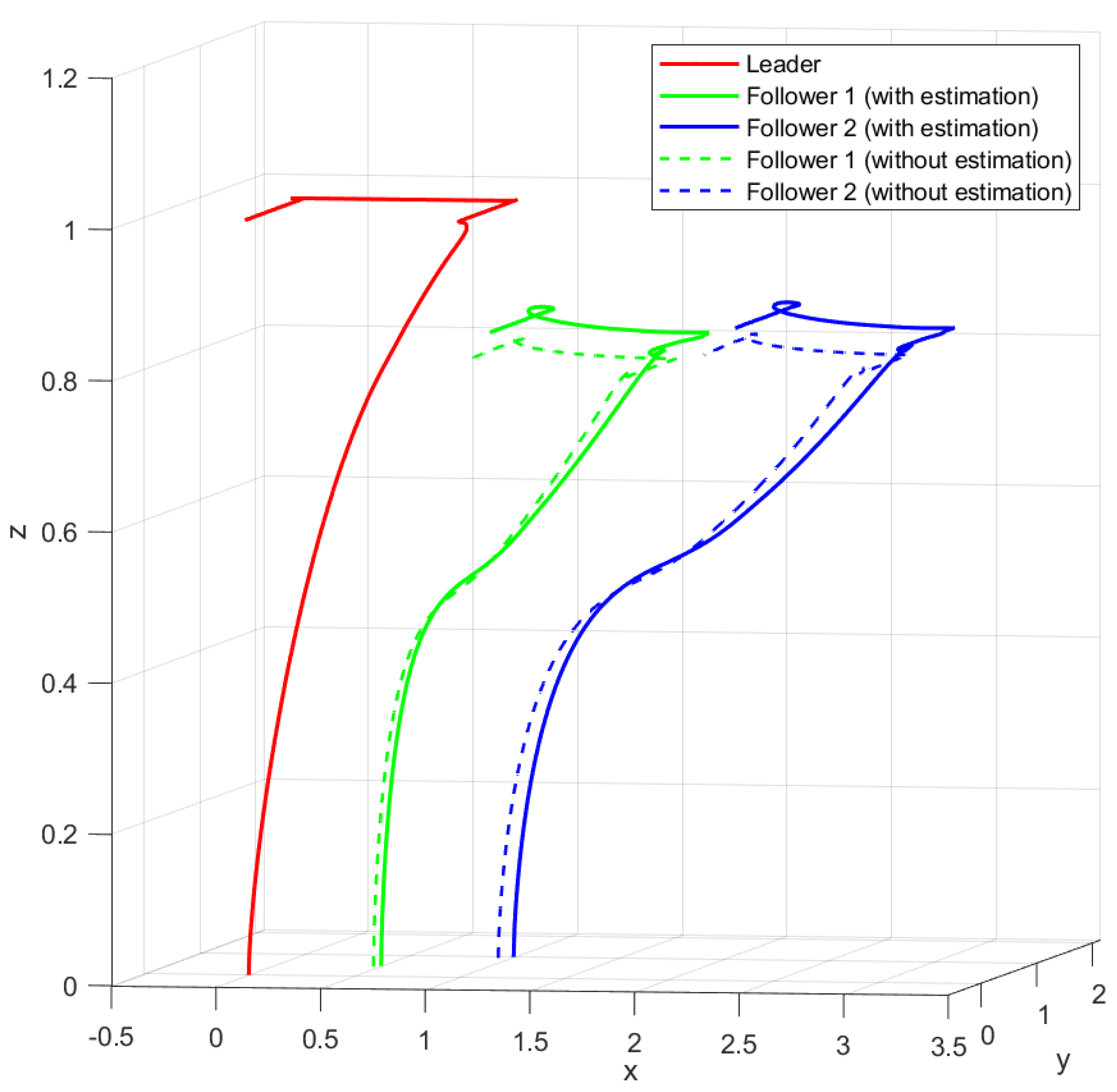
The leader UAV was commanded to follow a dynamic trajectory composed of four connected linear segments, maintaining a constant altitude of 1 m throughout the maneuver. As shown in Figure 3, it moves from $(0,0,0)$ to $(1,0,1)$ between 0 and 4 s, then to $(1,1,1)$ from 4 to 8 s, shifts to $(0,1,1)$ between 8 and 14 s, and finally returns to $(0,0,1)$ from 14 to 17 s.

While the leader follows this predefined path, follower UAVs 1 and 2 maintain fixed relative distances with respect to the leader, as specified in

Table 2. Relative distances of followers to the leader.

UAV	Distance in X (m)	Distance in Y (m)	Distance in Z (m)
Follower 1	1.0	0.5	0.2
Follower 2	2.0	0.1	0.2

.

The initial conditions for the UAVs were set as shown in

Table 3. Initial conditions for UAVs.

UAV	Position (m)	Velocity (m/s)	Orientation (rad)	Angular Velocity (rad/s)
Leader	(0, 0, 0)	(0, 0, 0)	(0, 0, 0)	(0, 0, 0)
Follower 1	(0.5, 0.5, 0)	(0, 0, 0)	(0, 0, 0)	(0, 0, 0)
Follower 2	(1, 1, 0)	(0, 0, 0)	(0, 0, 0)	(0, 0, 0)

.

Figure 3, Figure 4 and Figure 5 illustrate a comparative analysis of the proposed control strategy with and without the integration of HOSM estimators for external disturbances and parametric variations.

In Figure 3, the 3D trajectories reveal that the follower UAVs operating without estimators exhibit noticeable deviations from their desired formation positions, particularly during directional changes. These deviations result from unmodeled dynamics and external wind forces that the non-estimating controller fails to reject effectively. In contrast, the followers using estimators maintain their relative positions more accurately, validating the compensatory action provided by the integrated estimation scheme.

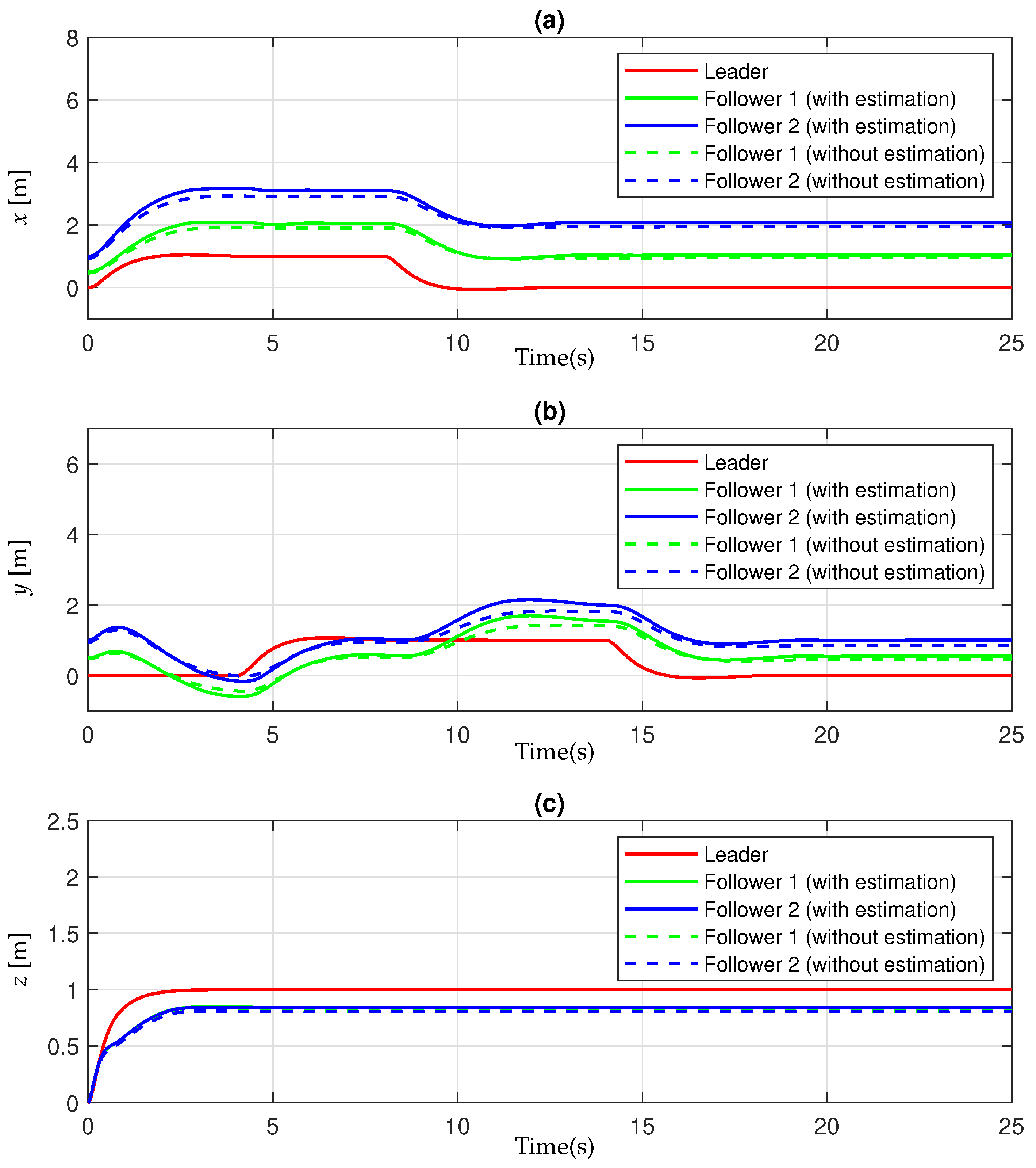
Figure 4 provides further insight by isolating the evolution of position components along the x-, y-, and z-axes. The followers without estimators exhibit larger tracking deviations, particularly during transient phases and directional changes, due to the compounded effect of parametric variations and wind disturbances. These deviations are more pronounced along the horizontal axes (subfigures (a) and (b)). In the vertical direction (subplot (c)), while all followers eventually converge to the desired altitude, those without estimation present a noticeable delay in alignment with the leader’s trajectory. In contrast, the estimators enhance the system’s ability to reject disturbances and maintain tighter formation across all axes. In contrast, the estimators enhance the system’s ability to reject disturbances and follow the leader’s trajectory more closely across all axes.

Figure 5 displays the tracking errors in relative positions between the followers and the leader. These errors are notably reduced when estimators are used. The absence of estimation leads to higher steady-state offsets, especially in the x-axis and y-axis tracking (subplots (a) and (b)). Despite disturbances, the proposed estimator-based approach demonstrates superior rejection capabilities, driving the tracking errors rapidly toward zero and ensuring tighter inter-agent coordination.

To further validate coordinated behavior, the evolution of orientation angles is presented in Figure 6. Subplot (a) shows the roll angle $\varphi$ and subplot (b) the pitch angle $\theta$ for all UAVs. All agents adjust their attitudes to match the leader’s angular profile, maintaining a synchronized orientation throughout the mission. The curves for followers 1 and 2 closely match the leader’s attitude, demonstrating that angular coordination is preserved even during aggressive maneuvers. The corresponding orientation tracking errors are shown in the second row of Figure 6. The plots represent the deviations $e_{\varphi }=\varphi -{\varphi }_d$ and $e_{\theta }=\theta -{\theta }_d$ over time. The controller efficiently drives both errors to zero, indicating the robust stabilization of the followers’ attitude dynamics. These results confirm that the proposed method guarantees consistent alignment in both position and orientation, which is crucial for tasks such as cooperative payload transport and aerial inspection.

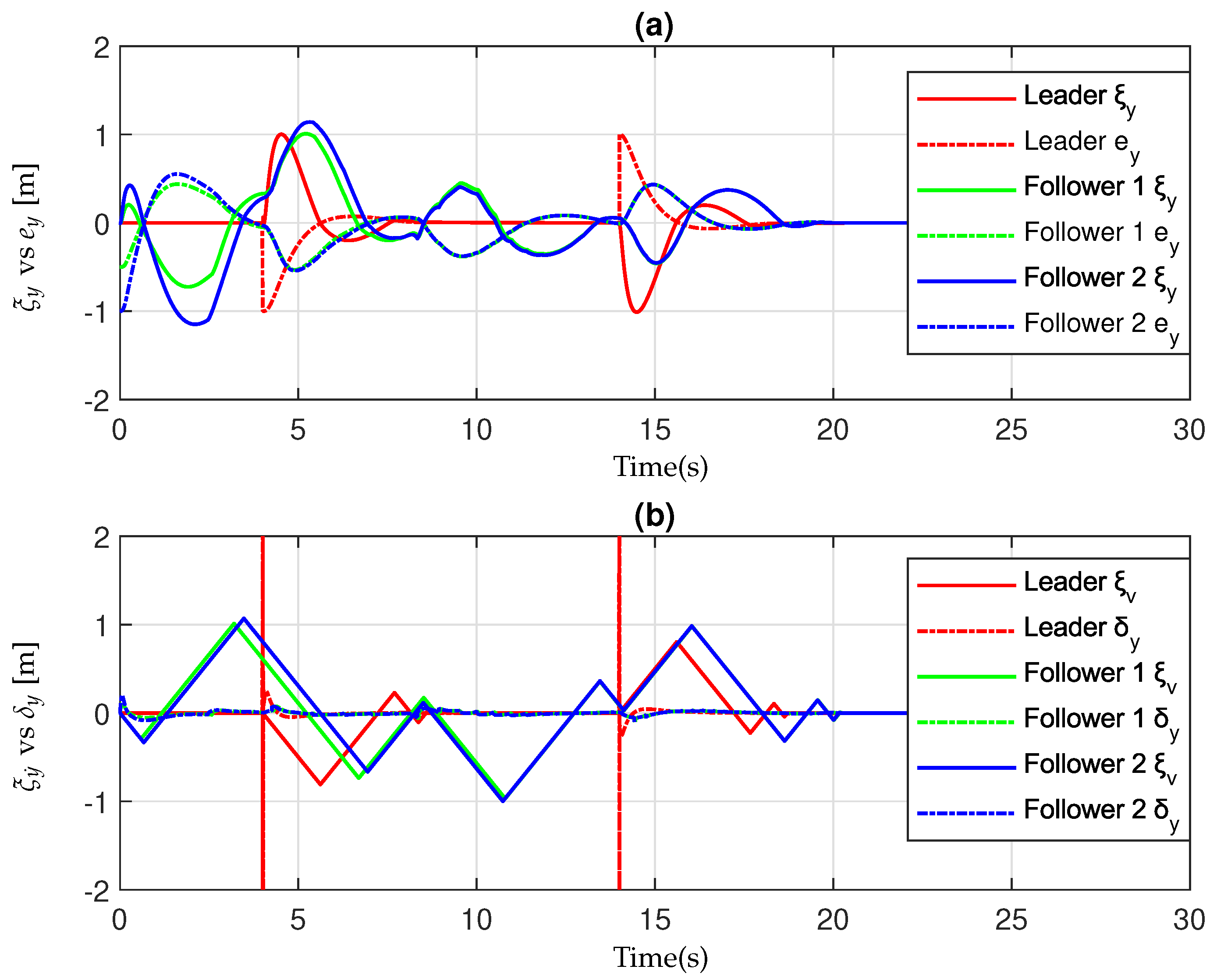
Finally, Figure 7, Figure 8 and Figure 9 evaluate the performance of the High-Order Sliding Mode estimators integrated into the control structure. Each figure contains two subplots: the top shows the estimator signals ${\xi }_x$, ${\xi }_y$, and ${\xi }_z$ against the corresponding tracking errors $e_x$, $e_y$, and $e_z$, while the bottom plots display ${\xi }_{\dot{x}}$, ${\xi }_{\dot{y}}$, and ${\xi }_{\dot{z}}$ against the estimated variations ${\delta }_x$, ${\delta }_y$, and ${\delta }_z$. Solid lines indicate the estimator outputs, while dash-dot lines represent the reference quantities. The convergence of estimator signals toward the actual tracking errors and system variations demonstrates the observer’s accuracy and robustness under measurement noise and modeling uncertainty. The estimators respond promptly to transient deviations and accurately reflect system behavior, enabling improved real-time compensation within the control loop.

Overall, the graphical results validate the proposed control architecture’s ability to ensure precise trajectory tracking, maintain geometric formation, compensate for dynamic uncertainties, and synchronize orientation—all under realistic disturbances and without sacrificing performance or stability.

6. Conclusions

In this paper, a robust formation control strategy for UAVs was developed to ensure precise relative positioning and trajectory adherence in three-dimensional space despite parametric uncertainties and external disturbances. The proposed approach, based on a backstepping framework with proportional-integral virtual controls, effectively stabilized tracking errors in the x-, y-, and z-axes, allowing the follower UAVs to maintain their formation relative to the leader.

To enhance the reliability of the assessment, a complex segmented 3D trajectory was introduced for the leader UAV, requiring coordinated responses from the followers in all spatial directions. The simulation results validated the proposed strategy by demonstrating accurate trajectory tracking, disturbance rejection, and adaptability to dynamic variations. The 3D trajectory plot and the tracking error estimations confirmed that the UAV system maintained stability and achieved the desired formation distances, even under significant disturbances.

Furthermore, the integration of translational and rotational dynamics, along with the decomposition of relative distances in the leader’s reference frame, improved the overall control precision. These results highlight the robustness and flexibility of the proposed control strategy, making it suitable for applications requiring multi-UAV coordination in dynamic environments.

While this work focused on the design and validation of a robust control strategy using HOSM-based estimators within a nonlinear framework, no direct comparisons with alternative controllers were included. As such, future work will aim to extend this approach to heterogeneous UAV formations, conduct comparative studies with other control techniques under the same full dynamic model, and implement real-time environmental sensing for improved adaptability in complex scenarios. In addition, the inclusion of vertical wind disturbances (z-component) will be investigated to further assess the system’s robustness under fully three-dimensional environmental conditions.

References

1. Nex, F.; Armenakis, C.; Cramer, M.; Cucci, D.A.; Gerke, M.; Honkavaara, E.; Kukko, A.; Persello, C.; Skaloud, J. UAV in the advent of the twenties: Where we stand and what is next. ISPRS J. Photogramm. Remote Sens. 2022, 184, 215–242. [Google Scholar] [CrossRef]
2. Sivakumar, M.; Tyj, N.M. A literature survey of unmanned aerial vehicle usage for civil applications. J. Aerosp. Technol. Manag. 2021, 13, e4021. [Google Scholar] [CrossRef]
3. Ali, Z.A.; Han, Z.; Masood, R.J. Collective motion and self-organization of a swarm of UAVs: A cluster-based architecture. Sensors 2021, 21, 3820. [Google Scholar] [CrossRef]
4. Han, W.; Wang, J.; Wang, Y.; Xu, B. Multi-UAV flocking control with a hierarchical collective behavior pattern inspired by sheep. IEEE Trans. Aerosp. Electron. Syst. 2024, 60, 2267–2276. [Google Scholar] [CrossRef]
5. Giacomossi, L.; Souza, F.; Cortes, R.G.; Cortez, H.M.M.; Ferreira, C.; Marcondes, C.A.C.; Loubach, D.S.; Sbruzzi, E.F.; Verri, F.A.N.; Marques, J.C.; et al. Autonomous and collective intelligence for UAV swarm in target search scenario. In Proceedings of the 2021 Latin American Robotics Symposium (LARS), 2021 Brazilian Symposium on Robotics (SBR), and 2021 Workshop on Robotics in Education (WRE), Natal, Brazil, 11–15 October 2021; pp. 72–77. [Google Scholar] [CrossRef]
6. Ju, C.; Son, H.I. Multiple UAV systems for agricultural applications: Control, implementation, and evaluation. Electronics 2018, 7, 162. [Google Scholar] [CrossRef]
7. Skorobogatov, G.; Barrado, C.; Salamí, E. Multiple UAV systems: A survey. Unmanned Syst. 2020, 8, 149–169. [Google Scholar] [CrossRef]
8. Gu, J.; Su, T.; Wang, Q.; Du, X.; Guizani, M. Multiple moving targets surveillance based on a cooperative network for multi-UAV. IEEE Commun. Mag. 2018, 56, 82–89. [Google Scholar] [CrossRef]
9. Araujo, J.F.; Sujit, P.B.; Sousa, J.B. Multiple UAV area decomposition and coverage. In Proceedings of the 2013 IEEE Symposium on Computational Intelligence for Security and Defense Applications (CISDA), Singapore, 16–19 April 2013; pp. 30–37. [Google Scholar] [CrossRef]
10. Shima, T.; Rasmussen, S. UAV Cooperative Decision and Control: Challenges and Practical Approaches; Society for Industrial and Applied Mathematics: Philadelphia, PA, USA, 2009. [Google Scholar] [CrossRef]
11. Zeng, Y.; Xu, J.; Zhang, R. Toward energy-efficient UAV communication: A survey of trajectory design and resource management. IEEE Commun. Surv. Tutor. 2019, 21, 1636–1672. [Google Scholar]
12. Nawaz, H.; Ali, H.M.; Laghari, A.A. UAV communication networks issues: A review. Arch. Comput. Methods Eng. 2021, 28, 1349–1369. [Google Scholar] [CrossRef]
13. Mohsan, S.A.H.; Othman, N.Q.H.; Li, Y.; Alsharif, M.H.; Khan, M.A. Unmanned aerial vehicles (UAVs): Practical aspects, applications, open challenges, security issues, and future trends. Intell. Serv. Robot. 2023, 16, 109–137. [Google Scholar] [CrossRef]
14. Zhou, B.; Wu, L.; Zhang, R.; Wang, H.; Zhang, Y. Multi-UAV network assisted intelligent edge computing: Challenges and opportunities. IEEE Netw. 2022, 36, 36–43. [Google Scholar] [CrossRef]
15. Zhao, X.; Zhang, Y.; Zhang, S.; Zhang, Y. Survey on mission planning of multiple unmanned aerial vehicles. Aerospace 2023, 10, 208. [Google Scholar] [CrossRef]
16. Bu, Y.; Yan, Y.; Yang, Y. Advancement Challenges in UAV Swarm Formation Control: A Comprehensive Review. Drones 2024, 8, 320. [Google Scholar] [CrossRef]
17. Do, M.T.; Hua, M.D. Formation Control Algorithms for Multiple-UAVs: A Comprehensive Survey. EAI Endorsed Trans. Ind. Netw. Intell. Syst. 2021, 8, e3. [Google Scholar] [CrossRef]
18. Zhang, Y.; Li, X.; Wang, J.; Zhang, Y. Collision Avoidance Mechanism for Swarms of Drones. Sensors 2023, 25, 1141. [Google Scholar] [CrossRef]
19. Li, H.; Wang, Y.; Zhang, R.; Wu, L. A Survey on Multiple Unmanned Vehicles Formation Control and Coordination: Current Status and Future Directions. Unmanned Syst. 2024, 12, 1–20. [Google Scholar] [CrossRef]
20. González-Sierra, J.; Dzul, A.; Martínez, E. Formation control of distance and orientation based-model of an omnidirectional robot and a quadrotor UAV. Robot. Auton. Syst. 2021, 143, 103921. [Google Scholar] [CrossRef]
21. Jiang, Y.; Bai, T.; Wang, Y. Formation Control Algorithm of Multi-UAVs Based on Alliance. Drones 2022, 6, 431. [Google Scholar] [CrossRef]
22. Vallejo-Alarcón, M.A.; Castro-Linares, R.; Velasco-Villa, M. Unicycle-Type Robot & Quadrotor Leader-Follower Formation Backstepping Control. IFAC-PapersOnLine 2015, 48, 51–56. [Google Scholar] [CrossRef]
23. Mercado-Ravell, D.; Castro, R.; Lozano, R. Quadrotors flight formation control using a leader-follower approach. In Proceedings of the European Control Conference (ECC), Zurich, Switzerland, 17–19 July 2013; pp. 3855–3860. [Google Scholar] [CrossRef]
24. Liu, C.; Xie, F.; Ji, T. Fixed-Wing UAV Formation Path Planning Based on Formation Control: Theory and Application. Aerospace 2024, 11, 1. [Google Scholar] [CrossRef]
25. Imran, I.H.; Kurtulus, D.F.; Memon, A.M.; Goli, S.; Kouser, T.; Alhems, L.M. Distributed Robust Formation Control of Heterogeneous Multi-UAVs with Disturbance Rejection. IEEE Trans. Aerosp. Electron. Syst. 2024, 12, 55326–55341. [Google Scholar] [CrossRef]
26. Liu, H.; Ma, T.; Lewis, F.L.; Wan, Y. Robust Formation Control for Multiple Quadrotors with Nonlinearities and Disturbances. IEEE Trans. Control Syst. Technol. 2018, 26, 427–438. [Google Scholar] [CrossRef]
27. Jasim, W.; Gu, D. Robust Team Formation Control for Quadrotors. IEEE Trans. Aerosp. Electron. Syst. 2017, 53, 3440–3452. [Google Scholar] [CrossRef]
28. Wang, Z.; Wang, T.; Li, T.; Mao, Z. Distributed observer-based close formation control for UAV swarm under outside disturbances and wake interferences. J. Frankl. Inst. 2024, 361, 106651. [Google Scholar] [CrossRef]
29. Li, J.; Liu, J.; Huangfu, S.; Cao, G.; Yu, D. Leader-follower formation of light-weight UAVs with novel active disturbance rejection control. Appl. Math. Model. 2022, 106, 357–374. [Google Scholar] [CrossRef]
30. Xu, L.-X.; Wang, Y.-L.; Wang, X.; Peng, C. Distributed Active Disturbance Rejection Formation Tracking Control for Quadrotor UAVs. IEEE Trans. Neural Netw. Learn. Syst. 2023, 54, 4678–4689. [Google Scholar] [CrossRef] [PubMed]
31. Koksal, N.; An, H.; Fidan, B. Backstepping-based adaptive control of a quadrotor UAV with guaranteed tracking performance. ISA Trans. 2020, 105, 98–110. [Google Scholar] [CrossRef]
32. Wang, J.; Alattas, K.A.; Bouteraa, Y.; Mofid, O.; Mobayen, S. Adaptive finite-time backstepping control tracker for quadrotor UAV with model uncertainty and external disturbance. Aerosp. Sci. Technol. 2023, 133, 108088. [Google Scholar] [CrossRef]
33. Liu, K.; Wang, R. Antisaturation command filtered backstepping control-based disturbance rejection for a quadarotor UAV. IEEE Trans. Circuits Syst. II Express Briefs 2021, 68, 3577–3581. [Google Scholar] [CrossRef]
34. Bao, C.; Guo, Y.; Luo, L.; Su, G. Design of a fixed-wing UAV controller based on adaptive backstepping sliding mode control method. IEEE Access 2021, 9, 157825–157841. [Google Scholar] [CrossRef]
35. Xu, L.X.; Ma, H.J.; Guo, D.; Xie, A.H.; Song, D.L. Backstepping sliding-mode and cascade active disturbance rejection control for a quadrotor UAV. IEEE/ASME Trans. Mechatronics 2020, 25, 2743–2753. [Google Scholar] [CrossRef]
36. Nguyen, N.P.; Mung, N.X.; Thanh, H.L.N.N.; Huynh, T.T.; Lam, N.T.; Hong, S.K. Adaptive sliding mode control for attitude and altitude system of a quadcopter UAV via neural network. IEEE Access 2021, 9, 40076–40085. [Google Scholar] [CrossRef]
37. Baek, J.; Kang, M. A synthesized sliding-mode control for attitude trajectory tracking of quadrotor UAV systems. IEEE/ASME Trans. Mechatronics 2023, 28, 2189–2199. [Google Scholar] [CrossRef]
38. Shao, X.; Sun, G.; Yao, W.; Liu, J.; Wu, L. Adaptive sliding mode control for quadrotor UAVs with input saturation. IEEE/ASME Trans. Mechatronics 2021, 27, 1498–1509. [Google Scholar] [CrossRef]
39. Noordin, A.; Mohd Basri, M.A.; Mohamed, Z.; Mat Lazim, I. Adaptive PID controller using sliding mode control approaches for quadrotor UAV attitude and position stabilization. Arab. J. Sci. Eng. 2021, 46, 963–981. [Google Scholar] [CrossRef]
40. Rinaldi, M.; Primatesta, S.; Guglieri, G. A comparative study for control of quadrotor UAVs. Appl. Sci. 2023, 13, 3464. [Google Scholar] [CrossRef]
41. Cárdenas R, C.A.; Grisales, V.H.; Collazos Morales, C.A.; Cerón-Muñoz, H.D.; Ariza-Colpas, P.; Caputo-Llanos, R. Quadrotor modeling and a pid control approach. In Proceedings of the Intelligent Human Computer Interaction: 11th International Conference, IHCI 2019, Allahabad, India, 12–14 December 2019; Springer: Berlin/Heidelberg, Germany, 2020; pp. 281–291. [Google Scholar] [CrossRef]
42. Choi, J.; Cheon, D.; Lee, J. Robust landing control of a quadcopter on a slanted surface. Int. J. Precis. Eng. Manuf. 2021, 22, 1147–1156. [Google Scholar] [CrossRef]
43. Bianchi, D.; Di Gennaro, S.; Di Ferdinando, M.; Acosta Lúa, C. Robust control of UAV with disturbances and uncertainty estimation. Machines 2023, 11, 352. [Google Scholar] [CrossRef]
44. Guillén-Bonilla, J.T.; Vaca García, C.C.; Di Gennaro, S.; Sánchez Morales, M.E.; Acosta Lúa, C. Vision-Based Nonlinear Control of Quadrotors Using the Photogrammetric Technique. Math. Probl. Eng. 2020, 2020, 5146291. [Google Scholar] [CrossRef]
45. Acosta Lúa, C.; Vaca García, C.C.; Di Gennaro, S.; Castillo-Toledo, B.; Sánchez Morales, M.E. Real-Time Hovering Control of Unmanned Aerial Vehicles. Math. Probl. Eng. 2020, 2020, 2314356. [Google Scholar] [CrossRef]
46. Nagaty, A.; Saeedi, S.; Thibault, C.; Seto, M.; Li, H. Control and navigation framework for quadrotor helicopters. J. Intell. Robot. Syst. 2013, 70, 1–12. [Google Scholar] [CrossRef]
47. Beard, R.W.; McLain, T.W. Small Unmanned Aircraft: Theory and Practice; Princeton University Press: Princeton, NJ, USA, 2024. [Google Scholar]
48. Moreno, J.A.; Osorio, M. A Lyapunov Approach to Second–Order Sliding Mode Controllers and Observers. In Proceedings of the 47th IEEE Conf. Decision Control, Cancun, Mexico, 9–11 December 2008; pp. 2856–2861. [Google Scholar] [CrossRef]
49. Khalil, H.K. Nonlinear Systems; Prentice Hall: Saddle River, NJ, USA, 2006. [Google Scholar]
Figure 1. The quadrotor schematic.
Mathematics 13 01520 g001
Figure 2. Quadrotors Formation.
Mathematics 13 01520 g002
Figure 3. 3D position trajectories of the three UAVs under external disturbances and parametric variations, comparing the control performance with and without disturbance and parameter estimation.
Mathematics 13 01520 g003
Figure 4. Position trajectories along the (a) x-, (b) y-, and (c) z-axes for the three UAVs, comparing control with and without estimation of external disturbances and parametric variations.
Mathematics 13 01520 g004
Figure 5. Tracking errors along the (a) x-, (b) y-, and (c) z-axes for the three UAVs, comparing control with and without estimation of external disturbances and parametric variations.
Mathematics 13 01520 g005
Figure 6. Roll and pitch angle trajectories and tracking errors for the three UAVs. (a,b) show the roll angle ϕ and pitch angle θ , while (c,d) show the tracking errors e ϕ = ϕ ϕ d and e θ = θ θ d .
Mathematics 13 01520 g006
Figure 7. Estimation performance in the x-axis for the three UAVs. (a) ξ x vs. e x ; (b) ξ x ˙ vs. δ x .
Mathematics 13 01520 g007
Figure 8. Estimation performance in the y-axis for the three UAVs. (a) ξ y vs. e y ; (b) ξ y ˙ vs. δ y .
Mathematics 13 01520 g008
Figure 9. Estimation performance in the z-axis for the three UAVs. (a) ξ z vs. e z ; (b) ξ z ˙ vs. δ z .
Mathematics 13 01520 g009