1. Introduction
Over recent decades, deep learning has profoundly influenced various applications such as image processing and natural language processing. Recent advancements in deep learning have extended the application scope to address a broad spectrum of problems including scientific computation. Notably, physics-informed neural networks (PINNs) have emerged as a potent tool for solving partial differential equations (PDEs). PINNs offer a novel approach by eliminating the need for traditional discretization, characteristic of conventional numerical solvers. Unlike traditional methods, PINNs optimize model parameters based on the loss at each collocation point, thus operating entirely mesh-free. This methodology allows the training to be governed solely by physical laws, boundary conditions, and initial conditions, circumventing the dependence on extensive high-fidelity datasets typical of other deep learning models. Due to their mesh-free nature and high computational efficiency, PINNs have attracted increasing attention in scientific computation domains.
Introduced by Raissi et al. [
1], PINNs have revolutionized the solution of supervised learning tasks by incorporating laws of physics described by general nonlinear PDEs. Significant research in PINNs has focused on weighting loss terms, optimizing activation functions, gradient techniques, neural network architectures, and loss function structures. Haghighat et al. [
2] enhanced PINNs’ effectiveness through a multi-network model that accurately represents field variables in solid mechanics, employing separate networks for each variable for improved inversion and surrogate modeling. Innovative methods to enforce physical constraints have also been developed. Lu et al. [
3] introduced hard constraints using penalty and augmented Lagrangian methods to solve topology optimization, resulting in simpler and smoother designs for problems with non-unique solutions. Similarly, Basir and Senocak [
4] advocated for physics- and equality-constrained neural networks using augmented Lagrangian methods to better integrate residual loss and boundary conditions. Wang et al. [
5] outlined best practices that significantly enhance the training efficiency and accuracy of PINNs. These practices are benchmarked against challenging problems to gauge their effectiveness. Moreover, advanced sampling methods have been paid much attention, as the performance of trained PINNs is highly related to the selection of collocation points in the computational spatial and temporal space. Wu et al. [
6] explored the impact of various sampling strategies on inverse problems, particularly emphasizing the differential effects of non-uniform sampling on problem-solving efficacy. Wight and Zhao [
7] proposed an adaptive PINN approach to solve the Allen–Cahn and Cahn–Hilliard equations, utilizing adaptive strategies in space and time alongside varied sampling techniques. Similarly, Tang et al. [
8] developed a deep adaptive sampling method that employs deep generative models to dynamically generate new collocation points, thereby refining the training dataset based on the distribution of residuals. The field has seen the introduction of several specialized software packages designed to facilitate the application of PINNs to both forward and inverse PDE problems, such as SciANN [
9] and DeepXDE [
10]. These packages support a range of PINN variants like conservative PINNs (cPINNs) [
11] and Finite basis PINNs (FBPINNs) [
12], each tailored for specific scientific and engineering applications.
PINNs have demonstrated significant capabilities in addressing both forward and inverse modeling challenges. These networks effectively integrate data-driven learning with physics-based constraints, allowing them to handle complex problems in various scientific and engineering domains. Zhang et al. [
13] introduced a general framework utilizing PINNs to analyze internal structures and defects in materials, focusing on scenarios with unknown geometric and material parameters. This approach showcases PINNs’ utility in detailed material analysis and defect identification, which are critical in materials science and engineering. PINNs are increasingly recognized for their potential to expedite inverse design processes. As described by Wiecha et al. [
14], PINNs serve as ultra-fast predictors within optimization workflows, effectively replacing slower conventional simulation methods. This capability is pivotal in accelerating design cycles and enhancing efficiency in engineering tasks. Yago et al. [
15] successfully applied PINNs to the design of acoustic metamaterials, tackling complex topological challenges that require significant computational resources. This underscores PINNs’ effectiveness in domains demanding high computational power and intricate problem-solving capabilities. Meng et al. [
16] combined PINNs with the first-order reliability method to tackle the computationally intensive field of structural reliability analysis, highlighting the method’s potential to reduce computational burdens substantially.
Despite their successes, PINNs face several challenges such as high computational demands, difficulties in achieving convergence, nonlinearity, unstable performance, and susceptibility to trivial solutions. These issues often complicate their application in more complex scenarios. In response to these challenges, the classical numerical strategy of ‘divide and conquer’ [
17], traditionally employed to simplify complex analytical problems, has been adeptly adapted for use in PINNs. This approach involves decomposing the computational domain into smaller, more manageable subdomains. Each subdomain is modeled by a distinct neural network specifically tasked with approximating the PDE solution within that localized area. This method of localization substantially mitigates spectral bias inherent to neural networks, effectively reducing the complexity of the learning process by confining it to smaller domains. A foundational approach was outlined by Quarteroni and Valli, who provided deep insights into domain decomposition for PDEs [
18]. Building on these principles, Li et al. [
19] introduced the deep domain decomposition method (D3M) with a variational principle. Their methodology involves dividing the computational domain into several overlapping subdomains using the Schwarz alternating method [
17], enhanced by an innovative sampling method at junctions and a smooth boundary function. Jagtap and Karniadakis expanded on this by proposing spatial domain decomposition-based PINNs, specifically cPINNs and extended PINNs (XPINNs), which are tailored for various differential equations [
20]. Further advancements were made by Das and Tesfamariam, who developed a parallel PINN framework that optimizes hyperparameters within each subdomain [
21]. The utility of XPINNs in modeling multiscale and multi-physics problems was further emphasized by Hu et al. [
22] and Shukla et al. [
23], who also introduced augmented PINNs (APINNs) with soft domain decomposition to refine the XPINN approach. Additionally, domain decomposition has been successfully applied beyond traditional PINN applications. Bandai and Ghezzehei [
24] used it in PINNs to model water flow in unsaturated soils with discontinuous hydraulic conductivities. Meanwhile, Meng et al. [
25] explored the use of domain decomposition in a parallel PINN (PPINN) for time-dependent PDEs, employing a coarse-grained solver for initial model initialization followed by iterative refinements in each subdomain. Dwivedi et al. [
26] presented a distributed PINN approach, which entails dividing the computational domain into uniformly distributed non-overlapping cells, each equipped with a PINN. All PINNs are trained simultaneously by minimizing the total loss through a gradient descent algorithm. Stiller et al. [
27] trained individual neural networks to act as gates for distributing resources among expert networks in a Gated-PINN that utilizes domain decomposition. Li et al. [
28] introduced a deep-learning-based Robin–Robin domain decomposition method for Helmholtz equations, utilizing an efficient plane wave activation-based neural network to discretize the subproblems. They demonstrated that suitable Robin parameters on different subdomains maintain a nearly constant convergence rate despite an increasing wave number.
Notwithstanding the success of domain decomposition methods, significant challenges persist, particularly in dynamically adjusting interfaces and the number of subdomains. Currently, identifying the optimal decomposition strategy remains a largely unresolved issue, and intuitive engineering judgment often plays a crucial role alongside algorithms for efficient automatic decomposition [
29]. Moreover, state-of-the-art (SOTA) models are trained across the entire domain simultaneously, which can lead to significant computational waste if the models fail to converge in certain areas, resulting in considerable inefficiencies. This area remains ripe for further research and development, suggesting a critical direction for future investigations aimed at optimizing the efficiency and adaptability of these methods. This paper proposes a progressive domain decomposition (PDD) method that can effectively mitigate the aforementioned challenges by strategically and progressively partitioning the domain in accordance with the dynamics of residual loss. For static problems, the domain can be divided based on residual behaviors. In cases involving time evolution, it is also necessary to respect causality inherent in physics. There are two contributions presented by the PDD method. Residual dynamics precisely identify the key areas which need dense collocation samples, high computational power, and refined algorithms due to high complexity in physics. Such an approach simplifies the management of distinct models for various subdomains and reduces the need for sweeping hyperparameter adjustments across the entire model. Through the progressive saving of the trained models in individual subdomains, training efforts are respected in successful sections. The following sections are organized as follows:
Section 2 reviews the principles of PINNs and domain decomposition methods.
Section 3 describes the methodologies employed in this work, detailing the computational framework and algorithmic strategies. In
Section 4, the proposed domain decomposition approach, PDD, is applied to three distinct PDE problems, demonstrating its effectiveness and generalization.
Section 5 concludes the research and outlines future research directions.
3. Progressive Domain Decomposition
While domain decomposition in neural networks offers a promising pathway for enhancing PINN methodologies, it also poses several challenges. Firstly, there is no clear criterion for decomposition. Secondly, when training fails, the resources used in this failed training are wasted, leading to resource consumption until successful hyperparameters or decomposition is identified. To address these issues, this section proposes a method called progressive domain decomposition (PDD).
3.1. Overall Procedure of PDD
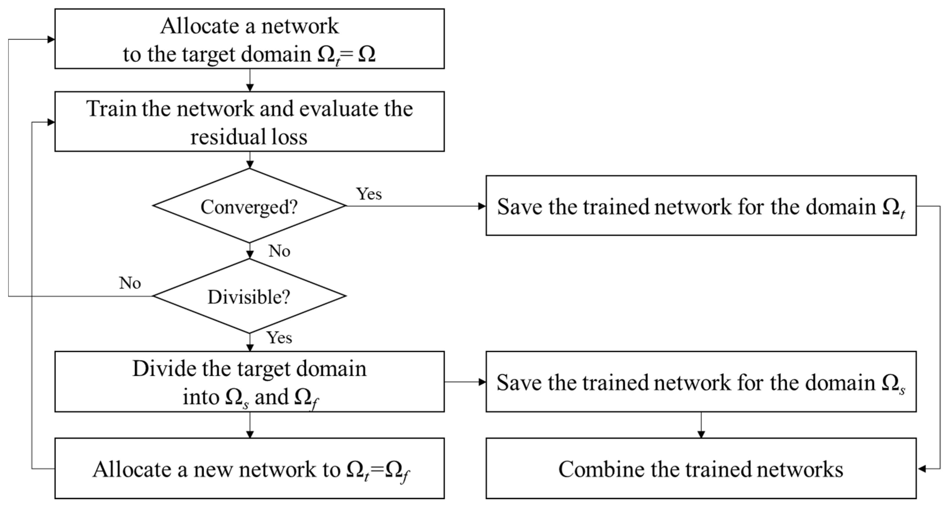
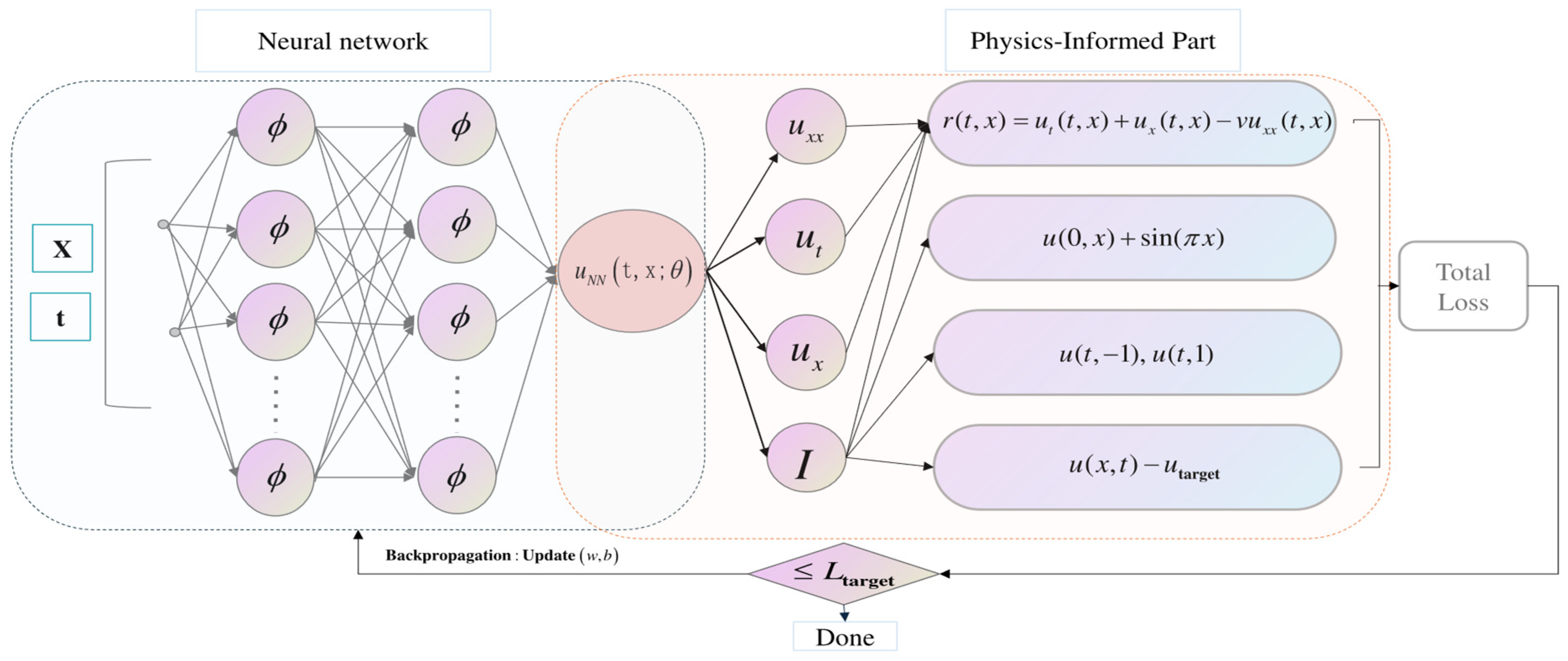
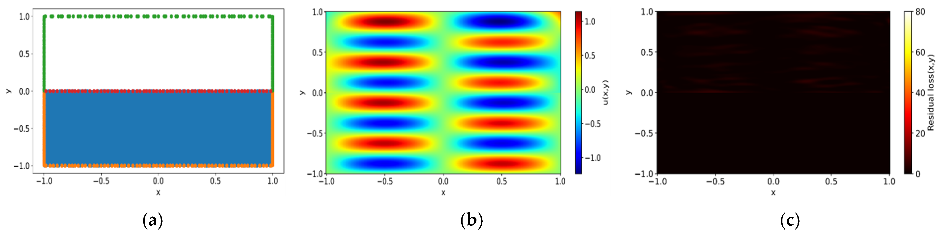
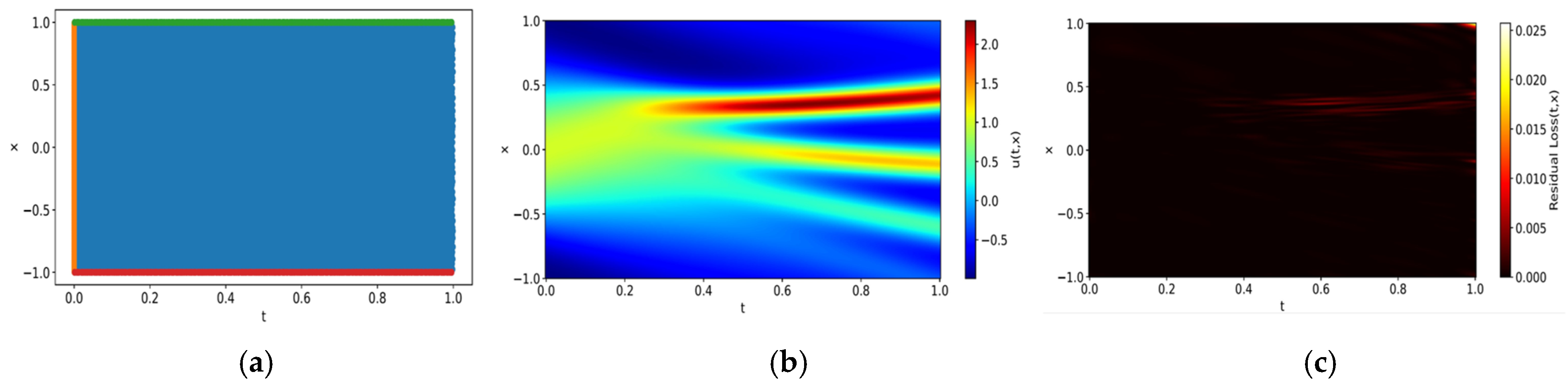
Figure 1 presents an overview of the suggested method. It starts with the assignment of a PINN to the target domain of the problem as in regular PINN training. The neural network is then trained to model the underlying physical phenomena within this domain. Upon completion of the training phase, the model undergoes an evaluation to assess residual loss. If the residual loss is small, it means that the network has been successfully trained with the initial setup. However, training is not always successful for various reasons [
32]. When training fails, it is common to re-evaluate and adjust the hyperparameters or network architecture and continue the training process. This cycle is repeated until the training is successfully completed, but all these steps contribute to increasing the overall cost of training.
On the other hand, when training fails, apart from cases where the model converges to a completely incorrect solution, it is common for some regions to achieve successful training while others do not. The proposed method leverages models that have successfully converged in these partial regions to improve overall training efficiency and accuracy. To achieve this, the computational domains are classified into , where training has succeeded, and , where training has failed, based on residual error analysis. The criteria for this classification will be discussed in the next section. For regions where training has succeeded, predictions are made using the existing neural network. Conversely, for regions where training has failed, a new neural network is assigned and trained. This adaptive strategy ensures that the learning process prioritizes regions with higher discrepancies, thereby enhancing the overall predictive accuracy. Moreover, it alleviates the challenge of hyperparameter tuning for the entire domain and eliminates the need to discard computational resources from the initial training phase. If a high-loss subdomain persists, it is further subdivided, and the iterative refinement process continues until all regions meet the desired accuracy threshold. Once this process is complete, the trained networks responsible for each subdomain are seamlessly integrated to form a unified global model. The existing networks and the newly trained networks communicate through three mechanisms. First, during training, the predictions from the existing networks at the interface serve as boundary conditions for the newly trained network, as the predictions of the existing networks are sufficiently accurate. Second, residual continuity and flux continuity are enforced to maintain consistency with the underlying physical principles. Third, once the newly created networks satisfy the convergence criteria, predictions at the interfaces between subdomains are computed as the weighted average of outputs from neighboring subdomains, as formulated in Equations (14) and (15). This approach ensures smooth transitions and consistency across the composite model. By mitigating boundary discrepancies, this framework enables the model to function as a cohesive and robust whole.
3.2. Criteria for Domain Decomposition
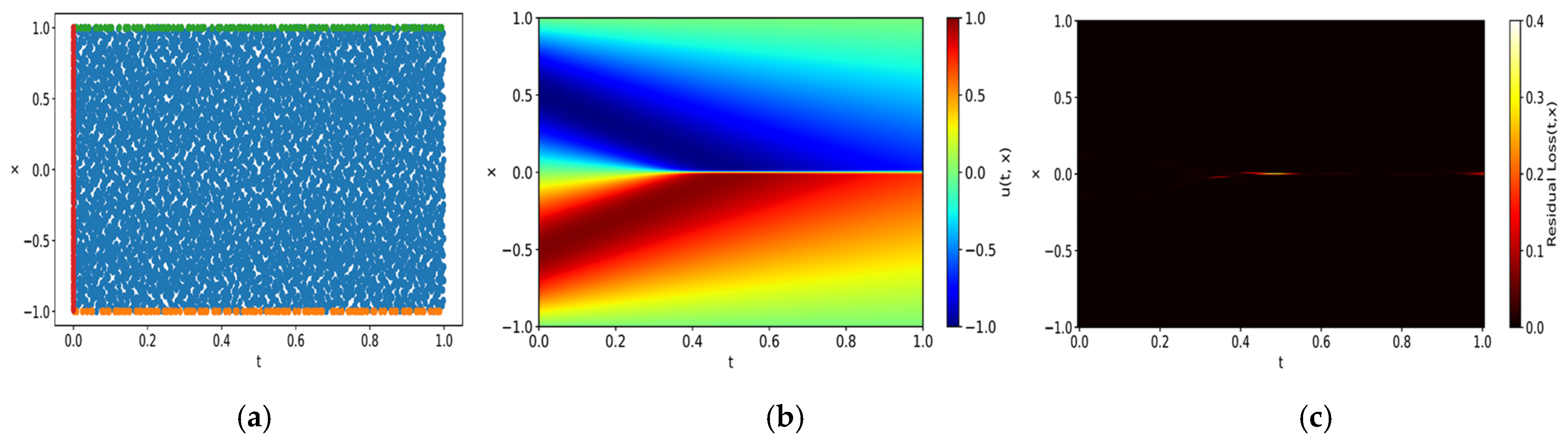
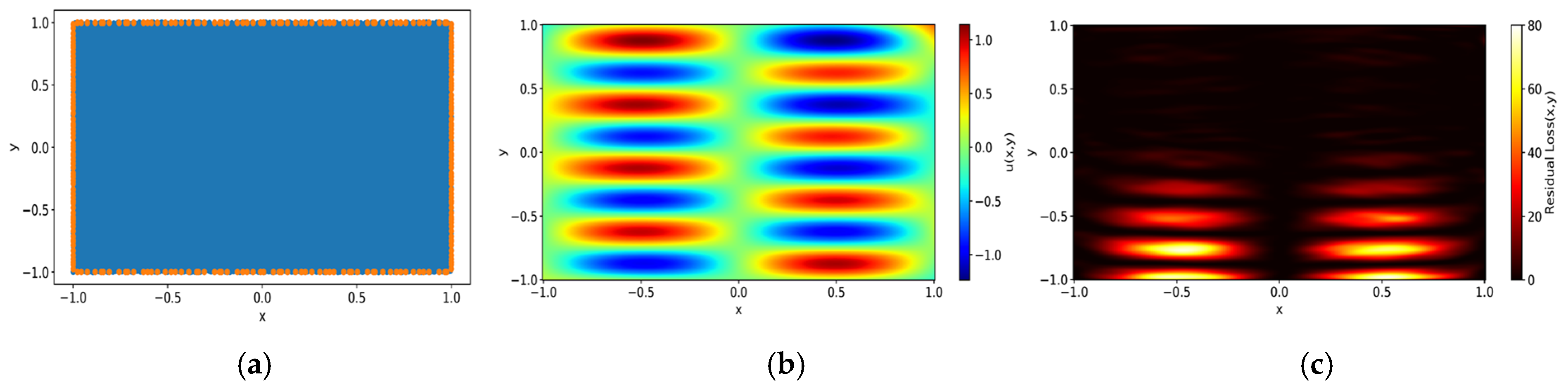
In the PDD framework, specific areas within the computational domain that disproportionately contribute to the overall error are identified, enabling targeted refinement and the more efficient allocation of computational resources. This identification process relies on a predefined threshold of residual loss, aimed at delineating areas where losses are concentrated relative to the entire domain.
For this purpose, residual loss data are collected from uniformly distributed points within the domain following model training. The domain is segmented into Ns subdomains
(
i = 1, …, Ns), and the residual loss for each subdomain is evaluated. The subdomain with the highest residual loss is first selected as a test domain
, and it is checked whether this subdomain satisfies the following three conditions:
where
represents the aggregated residual loss in
, and A represents the area of the domain indicated with the subscript. Thus, the first condition
indicates the proportion of the total residual loss contributed by
, while the second condition
represents the proportion of
in the entire domain, and the third condition
illustrates the concentration of residual loss. If
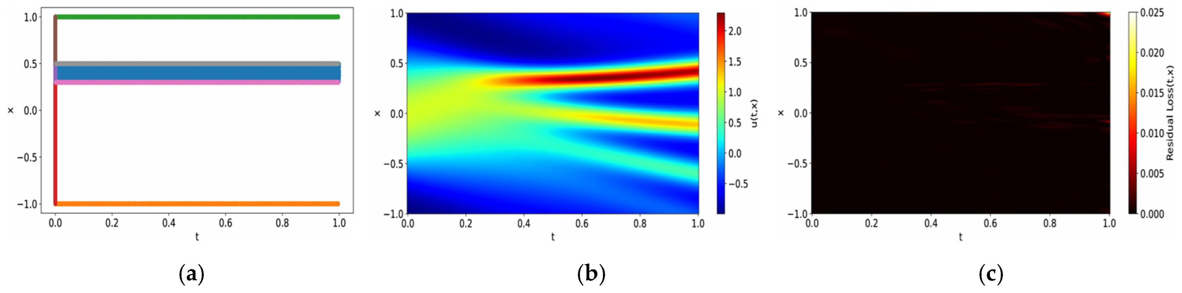
does not satisfy the conditions, an expanded test subdomain is formed by including neighboring subdomains. The new subdomain is determined by selecting the neighboring subdomain that shares a boundary and has the highest residual. This domain is then designated as the new test subdomain
. This process is repeated until the test subdomain meets the criteria. If the test subdomain satisfies the criteria, it is classified as a failed domain
, and the rest of the domain is classified as a successful domain
. The failed domain necessitates intensive analysis and additional training. A new network is assigned to the failed domain
for retraining. The subsequent process follows the method described in the previous section.
The reason for considering both the proportion of loss and the proportion of areas occupied by the test subdomain in defining the failed domain is to determine whether the loss is concentrated in a specific region. The proposed progressive domain decomposition method is appropriate only when the residual loss is concentrated in one area, and this criterion is used to measure that. If no region meets the criterion, this suggests a uniform distribution of residual losses across the domain, indicating that the model could benefit from comprehensive refinement instead of targeted intervention. In other words, hyperparameters or the network architecture should be adjusted, and the training process should be restarted to achieve better results.
Once a predefined convergence criterion is established, the objective is to reduce it to a level comparable to that of other subdomains. In this study, the thresholds for the conditions,
m,
n, and
t, are set to 0.4, 0.5, and 1.5, respectively. The convergence criterion of average residual loss
is determined as 10 times the average residual loss of the successful regions
as illustrated in Equation (19). A higher criterion is set for the retrained region because the failed subdomains often suffer from high complexity, discontinuities, or other challenging conditions that make achieving convergence more difficult. But by setting this criterion, we account for these challenges and provide a more realistic and achievable target for convergence.
Algorithm 1 provides a detailed definition of the PDD algorithm.
| Algorithm 1 Progressive Domain Decomposition |
| 1 | Input: Collect residual loss from N uniformly distributed points in the domain after training. |
| 2 | Segmentation: Divide the domain into subdomains and calculate the total residual loss: |
| 3 | High-Loss Detection: For each subdomain , identify the subdomain with the highest residual loss. Classify as high loss if it satisfies: and represents the residual loss in and denotes the subdomain area. |
| 4 | Expanded search (if needed): if does not meet the condition, expand the test subdomain by including the neighboring subdomain with the highest residual. Repeat until the conditions are met. |
| 5 | Classification: If satisfies the conditions, classify it as a failed domain ; remaining regions are classified as successful domain . Establish the convergence criterion as: , is the number of points in the successful subdomain. |
| 6 | Uniformity check: If no regions are flagged, consider global model refinement. |
| 7 | Neural Network Assignment: Assign a new neural network to ; continue using the existing network for . |
| 8 | Targeted Training: Train networks in until the residual loss satisfies: . |
| 9 | Re-evaluation: if , subdivide and repeat steps 3–7 for each new subdomain. |
| 10 | Model Composition: Combine trained networks from all subdomains into a single model; at subdomain interfaces, compute predictions by averaging outputs from adjacent subnetworks to ensure smooth transitions. |
| 11 | Output: Stop when all subdomains satisfy the condition: . |
5. Discussion
5.1. Limitations of the Proposed Neural Network Framework
While the PDD method has shown promising results in solving low-dimensional PDE problems, there are still challenges to address when scaling this approach to high-dimensional problems. One of the primary limitations is the computational expense that comes with finer segmentation of the domain, which can increase as the complexity of the problem grows. Additionally, managing communication between subdomains in high-dimensional settings can become increasingly difficult, especially when domains exhibit highly irregular geometries or complex boundary conditions. The effectiveness of the PDD method in such cases is still an open area for exploration. Future work should focus on refining domain segmentation techniques and improving interface management between subdomains to ensure smooth transitions and efficient model training for larger-scale problems.
5.2. Extensions of the PDD Approach
The PDD approach demonstrates great potential for extending the applicability of PINNs to more complex problems, particularly in higher-dimensional spaces. Combining PDD with other algorithms like cPINNs and XPNNs could significantly enhance the method’s ability to handle these challenges. Several state-of-the-art algorithms are designed to manage high-dimensional PDEs more effectively, offering a promising avenue for extending the scope of PDD beyond low-dimensional problems. Future research should focus on integrating these advanced neural network architectures and algorithms with PDD, ensuring that the method can handle a wider range of scientific and engineering applications while maintaining computational efficiency through dynamic subdomain pruning and parallel training protocols. Furthermore, while the current work focuses on static problems, the modular architecture of PDD provides a foundation for addressing time-dependent systems. By coupling the progressive training mechanism with the causal time-marching strategies in [
34], PDD can effectively model temporal evolution while maintaining its core advantages in domain decomposition. This hybrid paradigm would enable causal loss propagation through temporal residual evolution analysis, allowing the targeted refinement of subdomains during critical time intervals, and memory-efficient incremental updates to avoid retraining on full-domain data.
5.3. Special Challenges with the PDD Method
As the PDD method scales to more complex problems, several challenges remain. One major issue is the efficient identification and management of high-loss subdomains. While the method provides a strategy for handling regions with complex computational requirements, the dynamic adjustment of interfaces and the optimal partitioning of the domain remain unresolved. The increased complexity of high-dimensional problems further complicates interface communication, as the choice of continuity (solution, flux, or residual) must be adapted based on the specific characteristics of each subdomain. Developing more sophisticated strategies for managing these interfaces will be critical for improving the method’s performance in more intricate computational scenarios.
5.4. Methods for Communication at the Interface
Communication between subdomains is a critical factor for the success of the PDD method. The method must handle different types of continuity depending on the problem’s physical nature. In some cases, solution continuity is required to ensure consistency at the boundaries. For problems governed by conservation laws, such as fluid dynamics or heat transfer, flux continuity may be more appropriate. In other instances, residual continuity helps to reduce discrepancies at the interfaces, leading to more accurate and stable results. The dynamic selection of the appropriate type of continuity at each interface is vital for maintaining smooth transitions and ensuring the accuracy and efficiency of the method as it scales to more complex, higher-dimensional problems. However, through extensive experimentation, we observed that enforcing residual continuity at interfaces had a negligible impact on the final prediction accuracy while significantly increasing computational overhead during training. Consequently, our study intentionally omits residual continuity as a loss term to prioritize training efficiency without compromising accuracy. Instead, we enforced solution continuity and flux continuity at subdomain interfaces, which sufficed to ensure global accuracy, as evidenced by the <1% error deviation across all tested cases compared to scenarios with residual continuity. This design choice not only streamlined training but also isolated PDD’s contributions by avoiding confounding factors from mixed boundary constraints. While residual continuity could enhance local smoothness, our results demonstrate that PDD’s adaptive loss prioritization already achieves superior accuracy to baseline PINNs without additional continuity enforcement. We acknowledge the potential value of residual continuity for specific applications and will explore its integration in future work to address higher-order interface requirements.
5.5. Hyperparameter Tuning
In the current work, the values of m, n, and t (i.e., m = 0.4, n = 0.5, t = 1.5) were determined through iterative numerical experimentation to balance residual minimization and interface coupling. These parameters were validated through systematic performance evaluation across multiple PDE benchmarks, demonstrating stable convergence and accuracy within the problem regimes studied.
Looking ahead, we are actively investigating automated hyperparameter optimization to systematize parameter determination using methods such as genetic algorithms and Bayesian optimization. Furthermore, we propose to explore adaptive mechanisms that dynamically adjust m, n, and t during training based on gradient variance monitoring. These efforts will extend our framework’s capability toward self-optimizing domain decomposition in PINNs, ensuring broader applicability across complex engineering problems.
6. Conclusions
The PDD method effectively identifies regions of complex computation by aggregating the interval residual loss during the evaluation of the trained model. This approach not only significantly enhances prediction accuracy but also preserves computational resources by strategically saving the model corresponding to each specific subdomain. To the best of our knowledge, this is the first time that criteria for domain decomposition in PINNs have been proposed. The method demonstrates broad applicability across various complex PDEs, establishing it as a versatile tool in computational science. Despite its success, further research is warranted to explore the relationship between the complexity of the problems and their specific locations within the domain. Such studies are essential for refining the efficacy of the PDD method and expanding its applicability in more nuanced computational scenarios.
The integration of domain decomposition into PINN frameworks aligns well with traditional numerical methods, offering a promising avenue for simplifying the computational challenges associated with large and complex domains. This synergy between simple neural network architectures and established numerical techniques paves the way for more robust and efficient solutions in computational science and engineering. The PDD method demonstrates superior performance compared to single-domain computations by effectively balancing computational accuracy and efficiency. This method is broadly applicable across a variety of complex PDEs, making it a versatile tool. By segmenting the computational domain and leveraging trained models within specific subdomains, the PDD method significantly reduces computational effort. This strategic partitioning not only conserves resources but also enhances the precision and speed of problem-solving processes.
This work makes several significant contributions to the field. First, we enhance the training process through strategic subdomain segmentation. During training, the domain is divided into subdomains based on a rigorously defined criterion that evaluates the complexity of different regions. This approach allows for precise solutions in specific sections, enabling targeted model updates in regions with higher computational challenges. It simplifies the management of distinct models for each subdomain and reduces the need for sweeping adjustments to hyperparameters across the entire model.
Second, the method enables the progressive saving of training results within each subdomain, effectively conserving training effort. By treating training failures as valuable assets for future phases, this approach allows for more focused research on the most complex areas of the domain. Advanced architectural designs and innovative training methodologies are employed to overcome these challenges.
Furthermore, we integrate a sequential training methodology with PDD, optimizing the learning process and enabling more efficient progress through challenging regions.
Finally, we expand the applicability of neural networks in scientific computing. By applying this method, we address and solve problems that have traditionally been difficult for conventional neural networks. This not only demonstrates the versatility of neural networks in scientific applications but also broadens their scope in solving complex real-world problems.
Future research will explore the implementation of different network architectures and hyperparameters to further enhance the robustness and global applicability of the proposed method, paving the way for its use in a wider range of scientific and engineering problems.


