Efficient Numerical Quadrature for Highly Oscillatory Integrals with Bessel Function Kernels

Abstract

In this paper, we investigate efficient numerical methods for highly oscillatory integrals with Bessel function kernels over finite and infinite domains. Initially, we decompose the two types of integrals into the sum of two integrals. For one of these integrals, we reformulate the Bessel function $J_{\nu }(z)$ as a linear combination of the modified Bessel function of the second kind $K_{\nu }(z)$, subsequently transforming it into a line integral over an infinite interval on the complex plane. This transformation allows for efficient approximation using the Cauchy residue theorem and appropriate Gaussian quadrature rules. For the other integral, we achieve efficient computation by integrating special functions with Gaussian quadrature rules. Furthermore, we conduct an error analysis of the proposed methods and validate their effectiveness through numerical experiments. The proposed methods are applicable for any real number $\nu$ and require only the first $\lfloor \nu \rfloor$ derivatives of f at 0, rendering them more efficient than existing methods that typically necessitate higher-order derivatives.

1. Introduction

In this paper, we are concerned with the problem of evaluating highly oscillatory integrals with the Bessel function of the form

$$I_1[f]={\int }_0^{b}f(x)J_{\nu }(\omega x)dx,$$

(1)

$$I_2[f]={\int }_0^{\infty }f(x)J_{\nu }(\omega x)dx,$$

(2)

where $b>0,|\omega |\gg 1$, $\nu$ is an arbitrary non-negative real number, and $J_{\nu }(\omega x)$ is the Bessel function of the first kind of order $\nu$ [1] (p. 358). These integrals appear in many applications, such as scattering problems, image processing, optics, and astronomy [1,2,3,4]. When $\omega$ is large, the integrand integrals oscillate rapidly, making classical quadrature rules, such as Newton–Cotes, Gauss, Clenshaw–Curtis, and Fejér-type rules, inefficient for their approximation. Therefore, it is significant to develop new effective methods for such integrals.

The computation of highly oscillatory integrals has attracted significant attention, with various methods having been proposed. These include asymptotic methods [5,6,7,8], Levin-type method [9,10,11,12], Filon-type method [13,14,15,16,17,18,19,20,21,22,23,24], numerical steepest descent method (also called complexethod) [25,26,27,28,29,30,31,32,33], and so on. The steepest descent method, which has been widely applied to nonlinear problems including elliptic PDEs [34] and gradient flow systems [35,36], works particularly well for exponential kernels [26,29]. However, extending it to Bessel kernels remains challenging. These integrals are hard to solve analytically, and classical numerical methods are inaccurate for higher frequencies.

The numerical computation of oscillatory integrals with Bessel kernels has been extensively studied in the literature. Wong’s pioneering work [32] established an early Gaussian quadrature method by reformulating the integral as a linear combination of Hankel function integrals, resulting in two line integrals with positive weight functions connected to modified Bessel functions of the second kind. Subsequent developments by Xu and Xiang [24] introduced an algorithm for computing integrals of the form

$$I[f]={\int }_a^{b}f(x)H_{\nu }^{(1)}(\omega x)dx,\omega \gg 1.$$

(3)

where $H_{\nu }^{(1)}(x)$ represents Hankel functions of the first kind. Their approach innovatively combined the fast Fourier transform with special function theory through Meijer G-functions and Lommel functions.

Significant progress has also been made in evaluating Cauchy principal value integrals involving oscillatory functions. Various techniques [16,30,37,38] have been developed for such problems, with Wang and Zhang [31] particularly advancing the analysis and computation of Hilbert transforms with oscillatory trigonometric kernels

$$I[f]={\int }_0^{+\infty }{\displaystyle \frac{f(t)}{t-x}}{e}^{i\omega t}dt,\omega >0,x\ge 0.$$

(4)

Parallel developments by Xu and colleagues [31,39] have produced efficient methods for Hilbert transforms containing oscillatory Bessel functions

$$I[f]={\int }_0^{+\infty }{\displaystyle \frac{f(x)}{x-\tau }}{J}_{\nu }(\omega x)dx,0<\tau <+\infty .$$

(5)

However, these existing methods generally cannot be directly applied to the integral (1) and (2) considered in this work, with only limited studies addressing this specific formulation.

The development of numerical steepest descent methods for Bessel-type integrals has followed an evolutionary path. Chen’s initial work [40] established the framework for integrals with $a>0$, but proved inapplicable to the $a=0$ case. This limitation was partially addressed in [41], where the method was extended to $a=0$ but remained restricted to integer orders $\nu$. Xu and Milovanović [42] later proposed an alternative approach using Whittaker W function representations, achieving broader applicability to non-negative real $\nu$ while maintaining computational efficiency. The quantitative comparison of these methods with the proposed approach is summarized in

Table 1. Comparison of method requirements and capabilities.

Method	$\mathit{\nu }$ Range	Derivative	Computational Complexity
Method in [41]	Integer $\nu$	$2N+2$	Medium (polynomial evaluation)
Method in [42]	$\nu \ge 0$	$2N-1+\lceil \nu \rceil$	Medium (polynomial evaluation)
Our Method	Any real $\mathit{\nu }$	$\lfloor \mathit{\nu }\rfloor$	Low (explicit formula)

.

Recent methodological innovations have further expanded the capabilities for handling oscillatory Bessel integrals. Sakhi Zaman et al. [43] integrated Bessel function representations with Levin-type methods, albeit with limitations regarding singular integrands. Kang’s team [44] advanced these techniques by developing modified integration paths and enhanced steepest descent approaches for singular cases. Despite these advances, current methods remain constrained by either restrictive parameter requirements (particularly regarding $\nu$) or inadequate handling of singularities.

To overcome these challenges, this paper presents a novel numerical steepest descent method that is valid for any real $\nu$ and requires only the first $\lfloor \nu \rfloor$ derivatives of f at 0. Our approach exploits the connection between $J_{\nu }(x)$ and the modified Bessel function $K_{\nu }(x)$, transforming the problem into line integrals with exponential decay, which are efficiently approximated using tailored Gaussian quadrature rules. Theoretical and numerical results demonstrate the method’s superiority in accuracy and computational efficiency, particularly for large $\omega$.

The innovations of this paper are as follows: (1) it accommodates any real $\nu$, (2) it requires only $[\nu ]$ derivatives of f at 0 (fewer than [41,42]), and (3) it achieves higher efficiency through Gaussian quadrature applied to transformed integrals with exponential decay. This provides broader applicability and improved performance, particularly for large $\omega$.

2. Numerical Methods for the Integrals in (1) and (2)

This section focuses on the numerical methods for evaluating the integrals presented in Equations (1) and (2). Throughout this paper, we adopt the convention of using C and R to represent generic constants without distinguishing between their specific instances. Additionally, we define the principal value of the logarithm as $log(z)=log(|z|)+iarg(z)$.

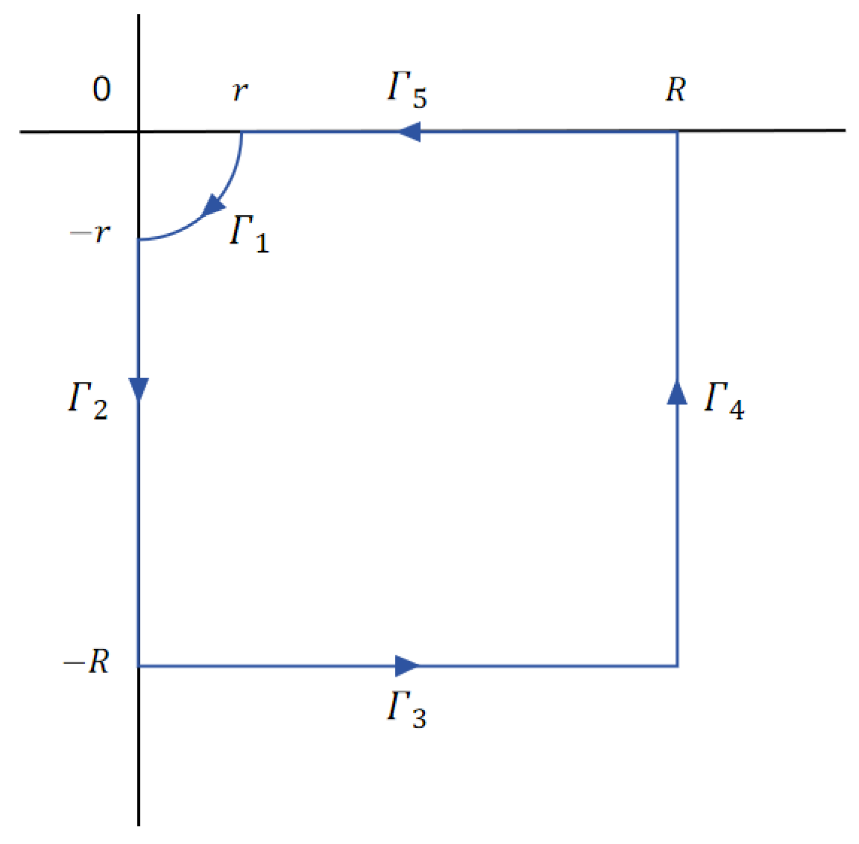
2.1. Complex Integration Method for the Integral $I_1[f]$

In this subsection, we propose an efficient method for the computation of integrals (1). We know that the Bessel function $J_{\nu }(z)$ is connected to the modified Bessel function $K_{\nu }(z)$ of the second kind by the relation [1]

$$i\pi J_{\nu }(z)=e^{-i\nu \pi /2}{K}_{\nu }(-iz)-e^{i\nu \pi /2}{K}_{\nu }(iz),|\mathrm{ph}z|\le {\displaystyle \frac{\pi }{2}}.$$

(6)

The new method proposed in this paper is based on this formula and the properties of $K_{\nu }(z)$. Without loss of generality, we assume that the function $f(x)$ is a real value function. The modified Bessel function $K_{\nu }(z)$ exhibits a singularity as $z\to 0$, with its asymptotic behavior given by [1]

$$K_{\nu }(x)\approx \left\{\begin{array}{cc}{\displaystyle \frac{1}{2}}\Gamma (\nu ){({\displaystyle \frac{x}{2}})}^{-\nu }\hfill & \Re (\nu )>0;\hfill \\ -ln(x)\hfill & \nu =0;\hfill \end{array}\right.z\to 0,$$

(7)

Together with the ideas in [41,42], we can rewrite the integral (1) as $I_1[f]=I_1^{\prime }[f]+I_1^{\prime \prime }[f]$. In this case, we define $I_1^{\prime }[f]$ and $I_1^{\prime \prime }[f]$ as

$$\begin{array}{cc}\hfill I_1^{\prime }[f]& ={\int }_0^b{x}^{\lfloor \nu \rfloor }{f}_{\nu }(x)J_{\nu }(\omega x)dx={\int }_0^b[f(x)-\sum _{k=0}^{\lfloor \nu \rfloor -1}{\displaystyle \frac{x^k}{k!}}{f}^{(k)}(0)]J_{\nu }(\omega x)dx,\hfill \\ \hfill I_1^{\prime \prime }[f]& ={\int }_0^b[f(x)-x^{\lfloor \nu \rfloor }{f}_{\nu }(x)]J_{\nu }(\omega x)dx={\int }_0^b\sum _{k=0}^{\lfloor \nu \rfloor -1}{\displaystyle \frac{x^k}{k!}}{f}^{(k)}(0)J_{\nu }(\omega x)dx,\hfill \end{array}$$

(8)

respectively, where $x^{\lfloor \nu \rfloor }{f}_{\nu }(x):=f(x)-{\sum }_{k=0}^{\lfloor \nu \rfloor -1}{\displaystyle \frac{x^k}{k!}}{f}^{(k)}(0)$, $[\nu ]$ denotes the greatest integer not more than $\nu$. The value of the integral $I_1^{\prime \prime }[f]$ can be evaluated analytically by

$$I_1^{\prime \prime }[f]={\int }_0^b\sum _{k=0}^{\lfloor \nu \rfloor -1}{\displaystyle \frac{f^{(k)}(0)}{k!}}{x}^k{J}_{\nu }(\omega x)dx=\sum _{k=0}^{\lfloor \nu \rfloor -1}{\displaystyle \frac{f^{(k)}(0)}{k!}}{\int }_0^b{x}^k{J}_{\nu }(\omega x)dx,$$

(9)

where ${\int }_0^b{x}^k{J}_{\nu }(\omega x)dx$ can be represented with a closed form [22]

$${\int }_0^b{x}^k{J}_{\nu }(\omega x)dx={\displaystyle \frac{2^k\Gamma (\frac{\nu +k+1}{2})}{{\omega }^{k+1}\Gamma (\frac{\nu -k+1}{2})}}+{\displaystyle \frac{b(k+\nu -1)}{{\omega }^k}}{J}_{\nu }(\omega b)s_{k-1,\nu -1}^{(2)}(\omega b)-{\displaystyle \frac{b}{{\omega }^k}}{J}_{\nu -1}(\omega b)s_{k,\nu }^{(2)}(\omega b),$$

(10)

where $s_{k,\nu }^{(2)}(z)$ is the Lommel function of the second kind which can be efficiently computed by the following truncation expansion [22] when z is large

$$s_{k,\nu }^{(2)}(z)=z^{k-1}[1+\cdots +{(-1)}^p{\displaystyle \frac{\{{(k-1)}^2-{\nu }^2\}\cdots \{{(k-2p+1)}^2-{\nu }^2\}}{z^{2p}}}]+O(z^{k-2p-2}),$$

(11)

For the integral $I_1^{\prime }[f]$, since $K_{\nu }(-iz)$ is the conjugate of $K_{\nu }(iz)$ for a real number z, we have

$${\int }_0^b{x}^{\lfloor \nu \rfloor }{f}_{\nu }(x)J_{\nu }(\omega x)dx=-{\displaystyle \frac{2}{\pi }}{\int }_0^b{x}^{\lfloor \nu \rfloor }{f}_{\nu }(x)\Im [e^{{\displaystyle \frac{\nu \pi i}{2}}}{K}_{\nu }(i\omega x)]dx,$$

(12)

In addition, as $f(x)$ is a real-valued function, we can simplify the integral to obtain

$${\int }_0^b{x}^{\lfloor \nu \rfloor }{f}_{\nu }(x)J_{\nu }(\omega x)dx=-{\displaystyle \frac{2}{\pi }}\Im [{\int }_0^b{x}^{\lfloor \nu \rfloor }{f}_{\nu }(x)e^{{\displaystyle \frac{\nu \pi i}{2}}}{K}_{\nu }(i\omega x)dx]$$

(13)

For convenience, we denote ${\mathcal{I}}_1[f_{\nu };\omega ]$ by

$${\mathcal{I}}_1[f_{\nu };\omega ]={\int }_0^b{x}^{\lfloor \nu \rfloor }{f}_{\nu }(x)K_{\nu }(i\omega x)dx,$$

(14)

We transform the integral into the following two line integrals

$${\mathcal{I}}_1[f_{\nu };\omega ]=-{\displaystyle \frac{i}{\omega }}{\int }_0^{\infty }{q}^{\lfloor \nu \rfloor }{f}_{\nu }(-{\displaystyle \frac{iq}{\omega }})K_{\nu }(q)dq+{\displaystyle \frac{i}{\omega }}{\int }_0^{\infty }{(b-{\displaystyle \frac{iq}{\omega }})}^{\lfloor \nu \rfloor }{f}_{\nu }(b-{\displaystyle \frac{iq}{\omega }})K_{\nu }(i\omega b+q)dq,$$

(15)

We denote the left-hand side of Equation (15) as ${\tilde{I}}^{\prime }[f]$ and the right-hand side as ${\tilde{I}}^{\prime \prime }[f]$, yielding the decomposition ${\mathcal{I}}_1[f_{\nu };\omega ]={\tilde{I}}^{\prime }[f]+{\tilde{I}}^{\prime \prime }[f]$. For the integrand ${\tilde{I}}^{\prime }[f]$, Gaussian quadrature with the weight function $q^{\lfloor \nu \rfloor }{K}_{\nu }(q)$ provides an efficient approximation. Due to the singularity of $K_{\nu }(q)$ at $q=0$, the Gauss–Laguerre quadrature rule is unsuitable. Instead, we evaluate ${\tilde{I}}^{\prime }[f]$ as follows

$${\tilde{I}}^{\prime }[f]\approx Q_{{\tilde{I}}^{\prime }[f]}^N={\displaystyle \frac{i}{\omega }}\sum _{k=1}^N{w}_k{(x_k)}^{\lfloor \nu \rfloor }{f}_{\nu }\left(-{\displaystyle \frac{i{x}_k}{\omega }}\right)K_{\nu }(x_k).$$

(16)

For the integrand ${\tilde{I}}^{\prime \prime }[f]$, the Gauss–Laguerre quadrature rule is applicable since $K_{\nu }(i\omega b+q)$ is nonsingular at $z=0$. Denoting this approximation by $\ddot{I}[f]$, we evaluate ${\tilde{I}}^{\prime \prime }[f]$ as follows:

$${\tilde{I}}^{\prime \prime }[f]\approx Q_{{\tilde{I}}^{\prime \prime }[f]}^N={\displaystyle \frac{i}{\omega }}\sum _{k=1}^N{w}_k{\left(b-{\displaystyle \frac{i{x}_k}{\omega }}\right)}^{\lfloor \nu \rfloor }{f}_{\nu }\left(b-{\displaystyle \frac{i{x}_k}{\omega }}\right)K_{\nu }(i\omega b+x_k).$$

(17)

While operator-based approximations (e.g., Bernstein–Kantorovich [45] and Bézier-type [46,47] operators) rely on polynomial basis adaptation, our method adopts a fundamentally different approach: Gaussian quadrature with orthogonal polynomials tailored to the oscillatory kernel $q^{|\nu |}{K}_{\nu }(q)$. This design avoids the saturation limits of classical operators and guarantees spectral accuracy for analytic integrands.

Then, we can rewrite $I[f]$ as

$$I[f]=-{\displaystyle \frac{2}{\pi }}\Im (e^{\nu \pi i/2}{\mathcal{I}}_1[f_{\nu };\omega ])+I_1^{\prime \prime }[f].$$

(18)

The modified Bessel function of the second kind $K_{\nu }(z)$ decays exponentially as $z\to \infty$ that can be seen from [1]

$$K_{\nu }(z)\sim \sqrt{\pi /(2z)}{e}^{-z},z\to \infty ,|phz|<{\displaystyle \frac{3}{2}}\pi .$$

(19)

By this character, $I_1[f]$ can be efficiently approximated by this new method with similar skills as in [1,26].

Theorem 1. 

Suppose that f is an analytic function in the infinity half-strip region of the complex plane $\{0\le \Re (z)\le b,\Im (z)\le 0\}$. If there are two constants M and ${\omega }_0$ such that for $0<{\omega }_0<\omega$

$$\begin{array}{c}\hfill |{\int }_0^{b}f(x+iR)dx|\le M{e}^{{\omega }_{0}R}\end{array}$$

(20)

then the integral ${\mathcal{I}}_1[f_{\nu };\omega ]$ can be transformed into two line integrals on the complex plane

$$\ddot{I}[f]=-{\displaystyle \frac{i}{\omega }}(I_1[f]-e^{-i\omega b}{I}_2[F])$$

(21)

where

$$I_1[F]={\int }_0^{\infty }F(-{\displaystyle \frac{iq}{\omega }})e^{-q}dq,I_2[F]={\int }_0^{\infty }F(b-{\displaystyle \frac{iq}{\omega }})e^{-q}dq$$

(22)

and

$$F(x)=f_{\nu }(x)K_{\nu }(i\omega x)e^{i\omega x}$$

(23)

Proof. 

The proof relies on Cauchy’s residue theorem [48,49], which states that for an analytic function in a simply connected domain, the integral along a closed contour equals the sum of residues inside. Here, we apply this theorem to the rectangular contour ${\Gamma }_1+{\Gamma }_2+{\Gamma }_3+{\Gamma }_4$ in the lower half-plane

$${\int }_{{\Gamma }_1+{\Gamma }_2+{\Gamma }_3+{\Gamma }_4}{f}_{\nu }(x)K_{\nu }(i\omega x)dx={\int }_{{\Gamma }_5}{f}_{\nu }(x)K_{\nu }(i\omega x)dx,$$

(24)

where all contours are oriented as shown in Figure 1. Since the integrand is analytic in this region, the left-hand side vanishes by Cauchy’s theorem.

Note that

$${\int }_{{\Gamma }_4}{f}_{\nu }(x)K_{\nu }(i\omega x)dx=i{\int }_0^R{f}_{\nu }(b-iq)K_{\nu }(i\omega b+\omega q)dq,$$

(25)

Similarly, we have

$${\int }_{{\Gamma }_3}{f}_{\nu }(x)K_{\nu }(i\omega x)dx={\int }_0^b{f}_{\nu }(s-iR)K_{\nu }(i\omega s+\omega R)ds,$$

(26)

For the integral over the contour ${\Gamma }_2$, yields

$${\int }_{{\Gamma }_2}{f}_{\nu }(x)K_{\nu }(i\omega x)dx=-i{\int }_r^R{f}_{\nu }(-iq)K_{\nu }(\omega q)dq,$$

(27)

Next, we consider the line integral on ${\Gamma }_1$

$${\int }_{{\Gamma }_1}{f}_{\nu }(x)K_{\nu }(i\omega x)dx={\int }_0^{-{\displaystyle \frac{\pi }{2}}}{f}_{\nu }(r{e}^{i\theta })K_{\nu }(i\omega r{e}^{i\theta })ir{e}^{i\theta }d\theta ,$$

(28)

together with the assumption of $f(x)$ and (7), we have

$$\underset{R\to \infty }{lim}{\int }_{{\Gamma }_3}{f}_{\nu }(x)K_{\nu }(i\omega x)dx=0.$$

(29)

Similarly, together with the assumption of $f(x)$ and (19), we obtain

$$\underset{r\to 0}{lim}{\int }_{{\Gamma }_1}{f}_{\nu }(x)K_{\nu }(i\omega x)dx=0.$$

(30)

Therefore, we can obtain the desired result by

$$\underset{R\to \infty ,r\to 0}{lim}{\int }_{{\Gamma }_1+{\Gamma }_2+{\Gamma }_3+{\Gamma }_4}{f}_{\nu }(x)K_{\nu }(i\omega x)dx=\underset{R\to \infty ,r\to 0}{lim}{\int }_{{\Gamma }_5}{f}_{\nu }(x)K_{\nu }(i\omega x)dx.$$

(31)

Thus, the proof is completed.  □

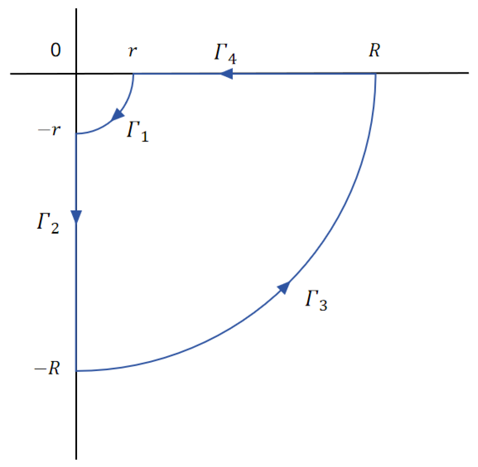
2.2. Complex Integration Method for the Integral $I_2[f]$

In this subsection, we consider the numerical evaluation of the oscillatory integral (2). Similar to the discussion above, we focus on the case where $\nu \ge 0$, although the new method presented in this paper is also valid for $\nu <0$ due to $K_{\nu }(z)=K_{-\nu }(z)$.

The case of $\mathbf{0}\le \mathit{\nu }<\mathbf{1}$: we begin by expressing the integral $I_2[f]$ in terms of the modified Bessel function $K_{\nu }(z)$. By equality (6), we have

$${\int }_0^{\infty }f(x)J_{\nu }(\omega x)dx={\displaystyle \frac{1}{i\pi }}{\int }_0^{\infty }f(x)\left[e^{-i\nu \pi /2}{K}_{\nu }(-i\omega x)-e^{i\nu \pi /2}{K}_{\nu }(i\omega x)\right]dx,$$

(32)

Since $K_{\nu }(-iz)$ is the conjugate of $K_{\nu }(iz)$ for a real number z, and $f(x)$ is a real-valued function, it yields

$${\int }_0^{\infty }f(x)J_{\nu }(\omega x)dx=-{\displaystyle \frac{2}{\pi }}\Im \left[{\int }_0^{\infty }f(x)e^{\nu \pi i/2}{K}_{\nu }(i\omega x)dx\right],$$

(33)

For convenience, we denote ${\mathcal{I}}_2[f;\omega ]$ by

$${\mathcal{I}}_2[f;\omega ]:={\int }_0^{\infty }f(x)K_{\nu }(i\omega x)dx,$$

(34)

then, we can rewrite (33)

$$I_2[f;\omega ]=-{\displaystyle \frac{2}{\pi }}\Im (e^{\nu \pi i/2}{\mathcal{I}}_2[f;\omega ]).$$

(35)

Theorem 2. 

Suppose that f is an analytic function in the infinity half-strip region of the complex plane $\{0\le \Re (z),\Im (z)\le 0\}$. If there are two constants M and ${\omega }_0$ such that for $0<{\omega }_0<\omega$

$$|{\int }_0^{b}f(x+iR)dx|\le M{e}^{{\omega }_{0}R}$$

then, the integral ${\mathcal{I}}_2[f;\omega ]$ can be transformed into line integrals on the complex plane for $0\le \nu <1$

$${\mathcal{I}}_2[f;\omega ]=-{\displaystyle \frac{i}{\omega }}{\int }_0^{\infty }f(-{\displaystyle \frac{iq}{\omega }})K_{\nu }(q)dq$$

(36)

Proof. 

By Cauchy’s residue theorem, we have

$${\int }_{{\Gamma }_1+{\Gamma }_2+{\Gamma }_3}f(x)K_{\nu }(i\omega x)dx={\int }_{{\Gamma }_4}f(x)K_{\nu }(i\omega x)dx,$$

(37)

with all contours taken in the directions that are depicted in Figure 2.

Note that

$${\int }_{{\Gamma }_1}f(x)K_{\nu }(i\omega x)dx={\int }_0^{-{\displaystyle \frac{\pi }{2}}}f(r{e}^{i\theta })K_{\nu }(i\omega r{e}^{i\theta })ir{e}^{i\theta }d\theta ,$$

(38)

by the weak singularity at 0 for $K_{\nu }(x)$ when $0\le \nu <1$ that can be seen in (9), we have the following result:

$$\underset{r\to 0}{lim}{\int }_{{\Gamma }_1}f(x)K_{\nu }(i\omega x)dx=\underset{r\to 0}{lim}{\int }_0^{-{\displaystyle \frac{\pi }{2}}}f(r{e}^{i\theta })K_{\nu }(i\omega r{e}^{i\theta })ir{e}^{i\theta }d\theta =0,$$

(39)

here, we used ${lim}_{r\to 0}{K}_{\nu }(i\omega r{e}^{i\theta })ir{e}^{i\theta }=0$.

Next, we consider the line integral on ${\Gamma }_3$

$${\int }_{{\Gamma }_3}f(x)K_{\nu }(i\omega x)dx={\int }_{-{\displaystyle \frac{\pi }{2}}}^{0}f(R{e}^{i\theta })K_{\nu }(i\omega R{e}^{i\theta })iR{e}^{i\theta }d\theta ,$$

(40)

Since (35), it yields

$$\underset{R\to \infty }{lim}{K}_{\nu }(i\omega R{e}^{i\theta })iR{e}^{i\theta }=0,-{\displaystyle \frac{\pi }{2}}\le \theta <0.$$

(41)

which means that

$$\underset{R\to \infty }{lim}{\int }_{{\Gamma }_3}f(x)K_{\nu }(i\omega x)dx=\underset{R\to \infty }{lim}{\int }_{-{\displaystyle \frac{\pi }{2}}}^{0}f(R{e}^{i\theta })K_{\nu }(i\omega R{e}^{i\theta })iR{e}^{i\theta }d\theta =0,$$

(42)

Together with (36), (38), and (40), we have

$$\begin{array}{ccc}\hfill {\int }_0^{\infty }f(x)K_{\nu }(i\omega x)dx& =& \underset{r\to 0,R\to \infty }{lim}{\int }_{{\Gamma }_2}f(x)K_{\nu }(i\omega x)dx\hfill \end{array}$$

(43)

$$\begin{array}{ccc}& =& -{\displaystyle \frac{i}{\omega }}{\int }_0^{\infty }f(-{\displaystyle \frac{iq}{\omega }})K_{\nu }(q)dq.\hfill \end{array}$$

(44)

Thus, the proof is completed.  □

The case of $\mathit{\nu }\ge \mathbf{1}$: For this case, we adopt the skill in [42], rewriting the integral $I_2[f;\omega ]$ in the following form:

$$I_2[f;\omega ]={\int }_0^{+\infty }f(x)J_{\nu }(\omega x)dx={\int }_0^{+\infty }{f}_e(x)e^{-x}{J}_{\nu }(\omega x)dx,$$

(45)

where $f_e(x)=f(x)e^x$. Let $\epsilon =\lfloor \nu \rfloor$ be the greatest integer less than or equal to $\nu$, and decompose $f_e(x)$ into a polynomial part $F_e(x)$ and a remainder $R_e(x)$

$$F_e(x):=e^{-x}\sum _{j=0}^{\epsilon -1}{\displaystyle \frac{f_e^{(j)}(0)}{j!}}{x}^j,R_e(x):=f(x)-F_e(x).$$

(46)

Therefore, we have

$$I_2[f;\omega ]={\int }_0^{+\infty }{F}_e(x)J_{\nu }(\omega x)dx+{\int }_0^{+\infty }{R}_e(x)J_{\nu }(\omega x)dx,$$

(47)

For the first integral in the right-hand side of the above equality, it can be expressed explicitly by the formula [50]

$$I_2[F_e;\omega ]={\int }_0^{+\infty }{F}_e(x)J_{\nu }(\omega x)dx=\sum _{j=0}^{\epsilon -1}{\displaystyle \frac{f_e^{(j)}(0)}{j!}}{\int }_0^{+\infty }{x}^j{e}^{-x}{J}_{\nu }(\omega x)dx,$$

(48)

where

$${\int }_0^{+\infty }{x}^j{e}^{-x}{J}_{\nu }(\omega x)dx={\left({\displaystyle \frac{\omega }{2}}\right)}^{\nu }{\displaystyle \frac{\Gamma (\nu +j+1)}{\Gamma (\nu +1)}}{}_{2}F_1\left({\displaystyle \frac{\nu +j+1}{2}},{\displaystyle \frac{\nu +j+2}{2}};\nu +1;-{\omega }^2\right),$$

(49)

where ${}_{2}F_1(a,b;c;z)$ is the hypergeometric function. Now, we return our attention to the second integral in the right-hand side of (47). Similarly, by using the conclusions from the previous subsection, it is easy to have

$$I_2[R_e;\omega ]=-{\displaystyle \frac{2}{\pi }}\Im (e^{\nu \pi i/2}{\mathcal{I}}_2[R_e;\omega ]).$$

(50)

and

$${\mathcal{I}}_2[R_e;\omega ]=-{\displaystyle \frac{i}{\omega }}{\int }_0^{\infty }{R}_e(-{\displaystyle \frac{iq}{\omega }})K_{\nu }(q)dq.$$

(51)

which can be effectively computed by a Gaussian quadrature rule

$${\mathcal{I}}_2[R_e;\omega ]\approx {\mathcal{Q}}_2^N[R_e;\omega ]=-{\displaystyle \frac{i}{\omega }}\sum _{j=1}^N{\widehat{w}}_j{R}_e\left(-{\displaystyle \frac{i{\widehat{x}}_j}{\omega }}\right){\left({\widehat{x}}_j\right)}^{-\epsilon }.$$

(52)

where ${\{{\widehat{x}}_j,{\widehat{w}}_j\}}_{j=1}^N$ are the nodes and weights of the Gaussian quadrature rule associated with the weight function $x^{\epsilon }{K}_{\nu }(x)$. Therefore, we give a new numerical method for computing the integral (2) for the case of $\nu \ge 1$

$$I_2[f;\omega ]\approx Q_2^N[f;\omega ]:=-{\displaystyle \frac{2}{\pi }}\Im \left(e^{\nu \pi i/2}{\mathcal{Q}}_2^N[R_e;\omega ]\right)+I_2[F_e;\omega ].$$

(53)

Similarly, it is easy to verify that the Formula (53) is also valid for the case of $0\le \nu <1$. In such a case, $\epsilon =0$ and $F_e(x)=0$. Therefore, for convenience, we regard Formula (53) as the new numerical method for approximating (2) in this paper.

3. Error Analysis of the Numerical Method for the Integral (1) and (2)

In this section, we discuss the asymptotic order with respect to $\omega$ for the presented methods (2). Since all the line integrals are approximated by Gauss-type quadrature rules, we introduce the following lemma.

Lemma 1 

(see [51]). Let $f\in C^{2N}[a,b]$. Then, the error for the Gaussian quadrature formula of order N is given by

$${\int }_a^{b}w(x)f(x)dx-\sum _{k=1}^N{w}_{k}f(x_k)={\displaystyle \frac{f^{(2N)}(\xi )}{(2N)!}}{\int }_a^{b}w(x){[q_N(x)]}^{2}dx$$

(54)

for some $\xi \in [a,b]$, where ${\{x_k,w_k\}}_{k=1}^N$ are Gaussian quadrature formula nodes and weights, $q_N(x)$ is the corresponding orthogonal polynomial of degree N associated with the weight function $w(x)$.

Using the above lemma, we can derive the asymptotic order on $\omega$ of the new numerical method (2).

Theorem 3. 

Suppose that f satisfied the conditions in Theorem 1. If $f^{(k)}(x)$ are bounded for $k=0,1,2,\cdots ,2N$, then the behavior of the numerical method (2) for approximating the integral (1) satisfies

$$E^N[f]:=|I[f]-Q_{I[f]}^N|=\left\{\begin{array}{cc}O({\omega }^{-2N-1}),\hfill & 0\le \nu <1;\hfill \\ O({\omega }^{-2N-1.5}),\hfill & \nu \ge 1;\hfill \end{array}\right.\omega \to \infty .$$

(55)

Proof. 

The errors of the new method for approximating the integral (1) are from the Gaussian quadrature rules for two line integrals on the complex plane. For the first line integral (35), by Lemma 1, we have

$${\int }_0^{\infty }{\displaystyle \frac{1}{q^{\epsilon }}}{R}_{\epsilon }^f(-{\displaystyle \frac{iq}{\omega }})q^{\epsilon }{K}_{\nu }(q)dq-\sum _{j=1}^N{\widehat{w}}_j{R}_{\epsilon }^f\left(-{\displaystyle \frac{i{\widehat{x}}_j}{\omega }}\right){\left({\widehat{x}}_j\right)}^{-\epsilon }=O\left({\displaystyle \frac{d{\left(\frac{1}{q^{\epsilon }}{R}_{\epsilon }^f(-\frac{iq}{\omega })\right)}^{2N}}{d^{2N}q}}{|}_{q=\xi }\right),$$

(56)

that is

$$O\left({\displaystyle \frac{1}{{\omega }^{\epsilon +2N}}}{\displaystyle \frac{d{\left(\frac{1}{q^{\epsilon }}{R}_n^f(-iq)\right)}^{2N}}{d^{2N}q}}{|}_{q={\displaystyle \frac{\xi }{\omega }}}\right)=O\left({\displaystyle \frac{1}{{\omega }^{\epsilon +2N}}}\right),$$

(57)

For the second line integral, using Lemma 1 as well, we have the following result:

$$\begin{array}{cc}\hfill & {\int }_0^{\infty }{R}_{\epsilon }^f(b-{\displaystyle \frac{iq}{\omega }})K_{\nu }(i\omega b+q)dq-\sum _{j=1}^N{w}_j^L{R}_{\epsilon }^f\left(b-{\displaystyle \frac{i{x}_j^L}{\omega }}\right)K_{\nu }(i\omega b+x_j^L)e^{x_j^L}\hfill \\ \hfill =& O\left({\displaystyle \frac{d{\left(R_{\epsilon }^f(b-\frac{iq}{\omega })K_{\nu }(i\omega b+q)e^q\right)}^{2N}}{d^{2N}q}}{|}_{q=\xi }\right),\hfill \end{array}$$

(58)

For the large $\omega$, according to the Formula (19), it follows

$$K_{\nu }(i\omega b+q)e^q\sim e^{-i\omega b}\sqrt{{\displaystyle \frac{\pi }{2(i\omega b+q)}}},$$

(59)

Figure 3 and Figure 4 display the real and imaginary parts of the function

$$g_{\nu ,\omega ,b}(q):=K_{\nu }(i\omega b+q)e^{i\omega b+q}\sqrt{{\displaystyle \frac{2(i\omega b+q)}{\pi }}},$$

(60)

Using (59), it is easy to show that

$$\begin{array}{cc}\hfill & O\left({\displaystyle \frac{d{\left(R_{\epsilon }^f(b-\frac{iq}{\omega })K_{\nu }(i\omega b+q)e^q\right)}^{2N}}{d^{2N}q}}{|}_{q=\xi }\right)=O\left({\displaystyle \frac{d{\left(R_{\epsilon }^f(b-\frac{iq}{\omega })\sqrt{\frac{\pi }{2(i\omega b+q)}}\right)}^{2N}}{d^{2N}q}}{|}_{q=\xi }\right)\hfill \\ \hfill & =O\left({\displaystyle \frac{1}{{\omega }^{2N+0.5}}}{\displaystyle \frac{d{\left(R_{\epsilon }^f(b-iq)\sqrt{\frac{\pi }{2(ib+q)}}\right)}^{2N}}{d^{2N}q}}{|}_{q={\displaystyle \frac{\xi }{\omega }}}\right)=O\left({\displaystyle \frac{1}{{\omega }^{2N+0.5}}}\right).\hfill \end{array}$$

(61)

Together with (56), (57), and (61), we can derive the desired results.

□

Theorem 4. 

Suppose that f satisfied the conditions in Theorem 2. If $f^{(k)}(x)$ are bounded for $k=0,1,2,\cdots ,2N$, then the behavior of the numerical method (53) for approximating the integral (2) satisfies

$$E_{\omega }^N[f]:=|I_2[f;\omega ]-Q_2^N[f;\omega ]|=\left\{\begin{array}{cc}O({\omega }^{-2N-1}),\hfill & 0\le \nu <1;\hfill \\ O({\omega }^{-2N-1-\lfloor \nu \rfloor }),\hfill & \nu \ge 1;\hfill \end{array}\right.\omega \to \infty .$$

(62)

Proof. 

The desired results can be derived easily from Lemma 1, (54). □

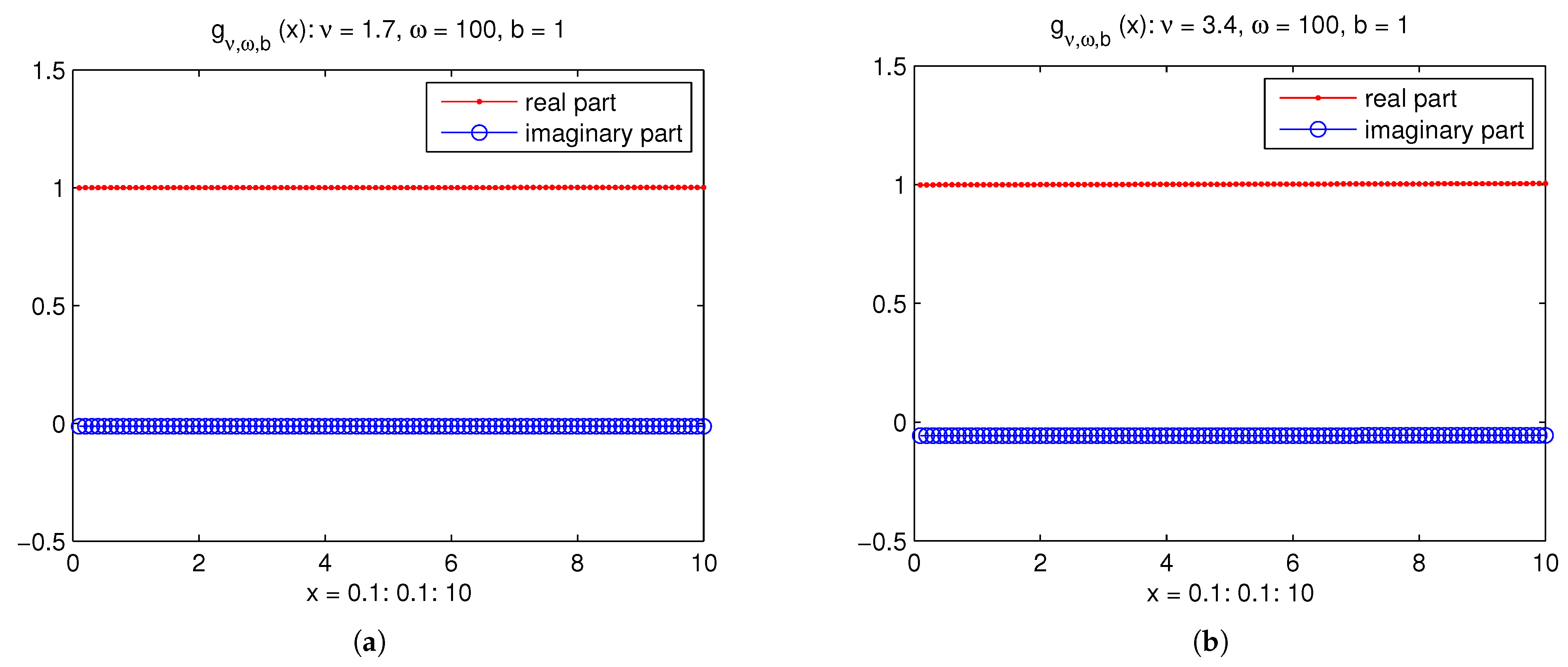
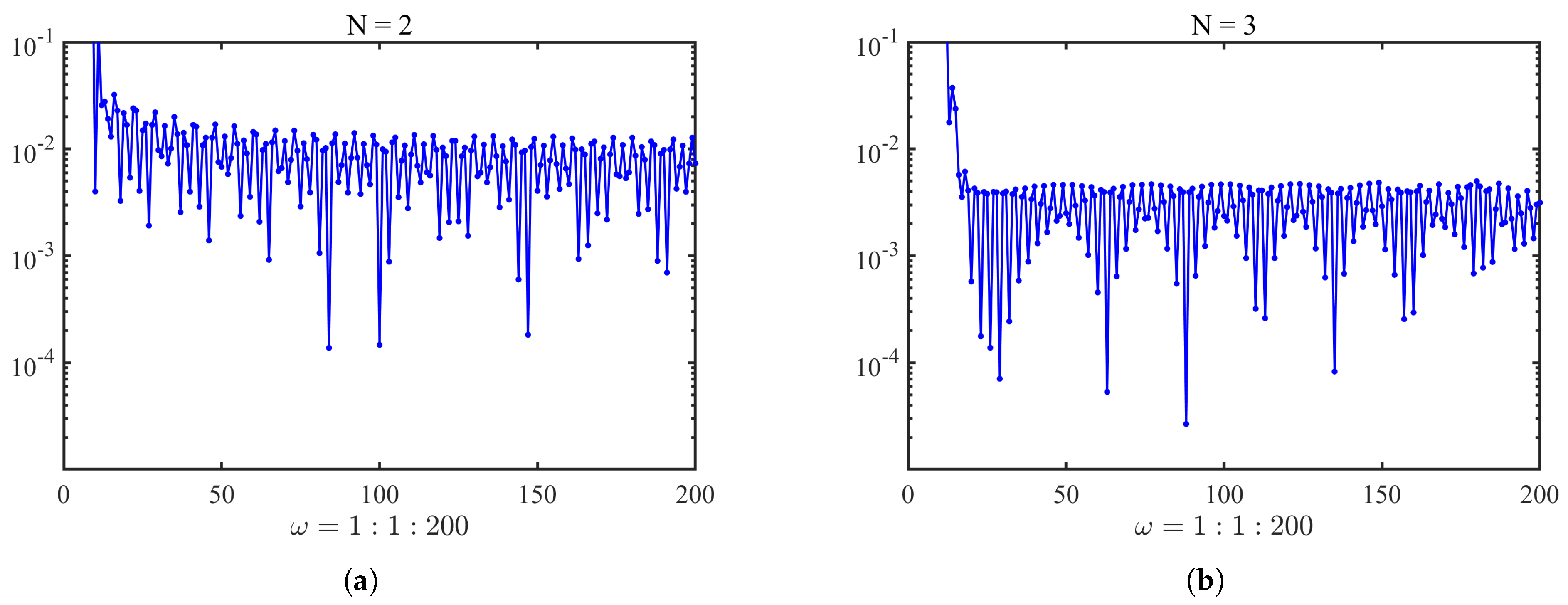
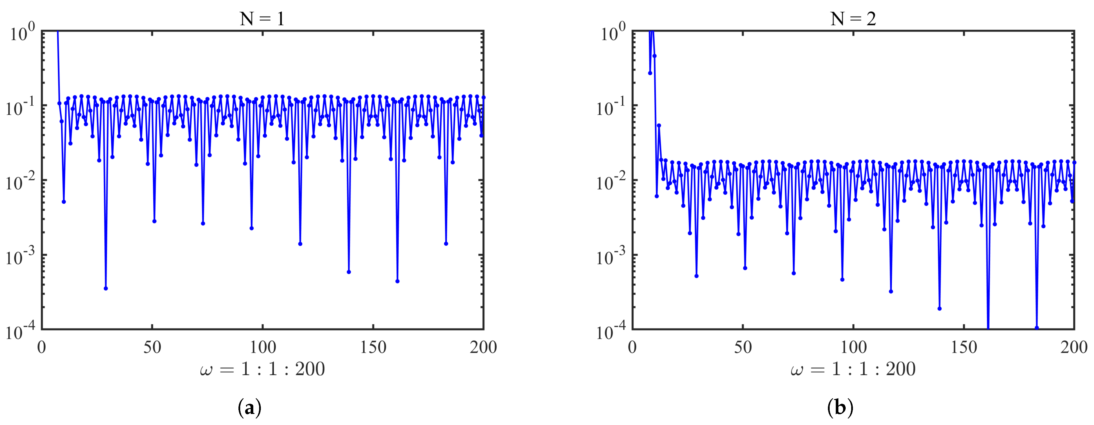
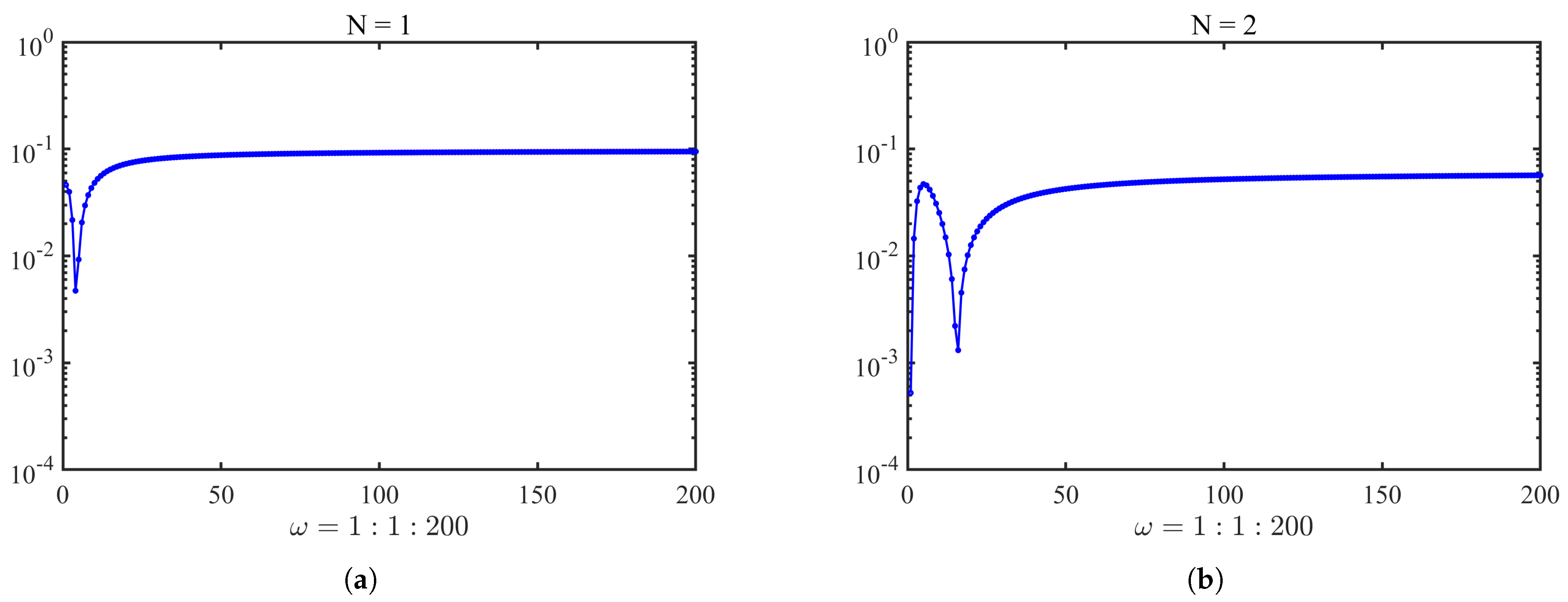
4. Numerical Examples

To illustrate the efficiency and accuracy of the new method described in Section 2, we give some numerical examples. In addition, we verify the asymptotic convergence order about $\omega$ in Theorems 3 and 4 by several numerical examples. The experiments are implemented on the R2013a version of the Matlab system. All the true values are obtained through Maple 17 with 32-digit arithmetic.

In this section, we present a series of numerical experiments to demonstrate the effectiveness of the new method. These examples demonstrate the effectiveness of our method for different values of $\nu$, particularly for both $\nu <1$ and $\nu \ge 1$. Additionally, we compare our method with the method proposed by Xu and Milovanović [42], highlighting the advantages of our approach, especially for $\nu \ge 1$. Finally, we provide visualizations of the error decay trends to further validate the theoretical error analysis.

Example 1. 

Let us consider the integral ${\int }_0^1{e}^x{J}_{\nu }(\omega x)dx$ with $\nu =0.3$ and $\nu =2.3$.

From the results in

Table 2. The absolute errors of the new method for approximating ${\int }_0^1{e}^x{J}_{0.3}(\omega x)dx$.

	$\mathit{\omega }={10}^2$	$\mathit{\omega }={10}^3$	$\mathit{\omega }={10}^4$
$N=2$	$1.79\times {10}^{-10}$	$6.49\times {10}^{-14}$	$3.99\times {10}^{-16}$
$N=3$	$6.51\times {10}^{-13}$	$4.29\times {10}^{-15}$	$1.33\times {10}^{-16}$
$N=4$	$1.10\times {10}^{-15}$	$2.21\times {10}^{-16}$	$2.66\times {10}^{-17}$
$N=5$	$3.31\times {10}^{-16}$	$2.21\times {10}^{-19}$	$1.99\times {10}^{-20}$

, the errors decrease rapidly as $\omega$ increases, and the method achieves machine precision even for small values of N. This demonstrates the effectiveness of our method for $0<\nu <1$ and $\nu \ge 1$.

Example 2. 

Let us consider the integral ${\int }_0^{\infty }{\displaystyle \frac{1}{1+x}}{J}_{\nu }(\omega x)dx$ with $\nu =0.6$ and $\nu =1.7$.

Similar to the previous example, the errors decrease rapidly as $\omega$ increases, and the method achieves high accuracy even for small N. As shown in

Table 3. The absolute errors of the new method for approximating ${\int }_0^1{e}^x{J}_{2.3}(\omega x)dx$.

	$\mathit{\omega }={10}^2$	$\mathit{\omega }={10}^3$	$\mathit{\omega }={10}^4$
$N=2$	$1.41\times {10}^{-10}$	$1.27\times {10}^{-15}$	$5.24\times {10}^{-16}$
$N=3$	$8.70\times {10}^{-15}$	$6.37\times {10}^{-16}$	$5.51\times {10}^{-17}$
$N=4$	$3.77\times {10}^{-16}$	$4.25\times {10}^{-16}$	$1.38\times {10}^{-17}$
$N=5$	$5.61\times {10}^{-17}$	$4.24\times {10}^{-17}$	$2.75\times {10}^{-19}$

,

Table 4. The absolute errors of the new method for approximating ${\int }_0^{\infty }{\displaystyle \frac{1}{1+x}}{J}_{0.6}(\omega x)dx$.

	$\mathit{\omega }={10}^2$	$\mathit{\omega }={10}^3$	$\mathit{\omega }={10}^4$
$N=2$	$1.12\times {10}^{-8}$	$1.30\times {10}^{-12}$	$8.25\times {10}^{-14}$
$N=3$	$6.72\times {10}^{-12}$	$4.43\times {10}^{-14}$	$2.71\times {10}^{-16}$
$N=4$	$6.28\times {10}^{-15}$	$4.33\times {10}^{-16}$	$5.42\times {10}^{-17}$
$N=5$	$1.74\times {10}^{-16}$	$4.34\times {10}^{-17}$	$3.21\times {10}^{-19}$

and

Table 5. The absolute errors of the new method for approximating ${\int }_0^{\infty }{\displaystyle \frac{1}{1+x}}{J}_{1.7}(\omega x)dx$.

	$\mathit{\omega }={10}^2$	$\mathit{\omega }={10}^3$	$\mathit{\omega }={10}^4$
$N=2$	$1.07\times {10}^{-9}$	$1.02\times {10}^{-14}$	$1.35\times {10}^{-15}$
$N=3$	$7.73\times {10}^{-13}$	$1.95\times {10}^{-15}$	$1.49\times {10}^{-16}$
$N=4$	$1.59\times {10}^{-15}$	$6.52\times {10}^{-16}$	$1.63\times {10}^{-17}$
$N=5$	$1.76\times {10}^{-16}$	$6.52\times {10}^{-17}$	$2.30\times {10}^{-19}$

, these results further validate the robustness of our method for both finite and infinite integration domains, particularly for different values of $\nu$.

These results illustrate that our method is robust and efficient for both $\nu <1$ and $\nu \ge 1$, making it a versatile tool for computing highly oscillatory integrals with Bessel function kernels.

To further validate the superiority of our method, we compare it with the method proposed by Xu and Milovanović [42] for the integral ${\int }_0^1{\displaystyle \frac{1}{1+{(1+x)}^2}}{J}_{1.6}(\omega x)dx$. The results are summarized in

Table 6. The absolute errors of the new method for approximating ${\int }_0^1{\displaystyle \frac{1}{1+{(1+x)}^2}}{J}_{1.6}(\omega x)dx$.

	Method	$\mathit{\omega }={10}^2$	$\mathit{\omega }={10}^3$	$\mathit{\omega }={10}^4$
$N=2$	Our method	$2.97\times {10}^{-11}$	$3.50\times {10}^{-14}$	$1.08\times {10}^{-15}$
	Method in [42]	$1.78\times {10}^{-2}$	$3.66\times {10}^{-4}$	$1.08\times {10}^{-6}$
$N=3$	Our method	$7.77\times {10}^{-14}$	$4.38\times {10}^{-16}$	$9.48\times {10}^{-16}$
	Method in [42]	$4.37\times {10}^{-3}$	$2.49\times {10}^{-5}$	$4.33\times {10}^{-6}$

, which shows the absolute errors of both methods for different values of $\omega$ and N.

Example 3. 

Let us consider the integral ${\int }_0^1{\displaystyle \frac{1}{1+{(1+x)}^2}}{J}_{\nu }(\omega x)dx$ with $\nu =1.6$.

Table 6 clearly demonstrates that our method outperforms Xu and Milovanović’s method, especially for larger values of $\omega$. For $\omega ={10}^3$ and $\omega ={10}^4$, our method achieves errors that are several orders of magnitude smaller than those of Xu and Milovanović’s method [42]. This is particularly significant for $\nu \ge 1$, where our method’s ability to handle higher-order Bessel functions without requiring additional derivatives provides a clear advantage.

To better demonstrate the error decay trends predicted by our theoretical analysis, we provide visualizations of the absolute errors scaled by ${\omega }^{2N+1}$ and ${\omega }^{2N+1.5}$ for different values of $\nu$ and N. These visualizations are presented in Figure 5, Figure 6, Figure 7, Figure 8, Figure 9 and Figure 10.

Figure 5 shows the error decay trends for $\nu <1$. The errors scaled by ${\omega }^{2N+1}$ exhibit a clear decay trend, confirming the theoretical error estimate of $O({\omega }^{-2N-1})$ for $\nu <1$.

Figure 6, Figure 7 and Figure 8 show the error decay trends for $\nu \ge 1$. The errors scaled by ${\omega }^{2N+1.5}$ and ${\omega }^{2N+1+\lfloor \nu \rfloor }$ demonstrate the expected decay trends, validating the theoretical error estimates of $O({\omega }^{-2N-1.5})$ and $O({\omega }^{-2N-1-\lfloor \nu \rfloor })$ for $\nu \ge 1$.

Figure 9 and Figure 10 further illustrate the error decay trends for integrals with infinite domains, showing that our method maintains its high accuracy and efficiency even for more challenging integrals.

These visualizations provide strong evidence that our method achieves the predicted error decay rates, further validating the theoretical analysis presented in Section 3.

5. Conclusions

In this paper, we propose an efficient numerical method for computing highly oscillatory integrals with Bessel function kernels, which are ubiquitous in wave propagation, acoustic scattering, and signal processing. By decomposing the integrals based on their domains and leveraging the connection between Bessel functions and modified Bessel functions, our method transforms the problem into efficiently computable forms using Gaussian quadrature and residue calculus. For finite domains, we achieve rapid convergence via Fourier-type integral representations, while for infinite domains, we combine quadrature rules with specialized function evaluations.

Our approach overcomes key limitations of existing methods: it applies to arbitrary real orders $\nu$, requires only the first $\lfloor \nu \rfloor$ derivatives of f at zero, and maintains high accuracy even for large frequencies $\omega$. Such improvements are particularly valuable in practical applications—for instance, in computational electromagnetics (e.g., Sommerfeld integrals in antenna theory) and seismic imaging, where Bessel-based oscillatory integrals arise frequently.

Future work will focus on extending the algorithm to higher-order Bessel kernels and oscillators with singularities, further broadening its applicability in scientific computing and engineering.

References

1. Olver, F.W.J.; Lozier, D.W.; Boisvert, R.F.; Clark, C.W. (Eds.) NIST Handbook of Mathematical Functions; Cambridge University Press: New York, NY, USA, 2010. [Google Scholar]
2. Bao, G.; Sun, W. A fast algorithm for the electromagnetic scattering from a large cavity. SIAM J. Sci. Comput. 2005, 27, 553–574. [Google Scholar] [CrossRef]
3. Duncan, D.B. Stability and convergence of collocation schemes for retarded potential integral equations. SIAM J. Numer. Anal. 2005, 42, 1167–1188. [Google Scholar]
4. Bisseling, R.; Kosloff, R. The fast Hankel transform as a tool in the solution of the time dependent Schrödinger equation. J. Comput. Phys. 1985, 59, 136–151. [Google Scholar] [CrossRef]
5. Erdélyi, A. Asymptotic representations of Fourier integrals and the method of stationary phase. J. Soc. Indust. Appl. Math. 1955, 3, 17–27. [Google Scholar] [CrossRef]
6. Iserles, A.; Nørsett, S.P. Efficient quadrature of highly oscillatory integrals using derivatives. Proc. R. Soc. A 2005, 461, 1383–1399. [Google Scholar] [CrossRef]
7. Iserles, A.; Nørsett, S.P. Quadrature methods for multivariate highly oscillatory integrals using derivatives. Math. Comput. 2006, 75, 1233–1258. [Google Scholar] [CrossRef]
8. Wang, H.; Xiang, S. Asymptotic expansion and Filon-type methods for a Volterra integral equation with a highly oscillatory kernel. IMA J. Numer. Anal. 2010, 31, 469–490. [Google Scholar] [CrossRef]
9. Levin, D. Procedures for computing one-and-two dimensional integrals of functions with rapid irregular oscillations. Math. Comput. 1982, 38, 531–538. [Google Scholar] [CrossRef]
10. Levin, D. Fast integration of rapidly oscillatory functions. J. Comput. Appl. Math. 1996, 67, 95–101. [Google Scholar] [CrossRef]
11. Levin, D. Analysis of a collocation method for integrating rapidly oscillatory functions. J. Comput. Appl. Math. 1997, 78, 131–138. [Google Scholar] [CrossRef]
12. Olver, S. Moment-free numerical integration of highly oscillatory functions. IMA J. Numer. Anal. 2006, 26, 213–227. [Google Scholar] [CrossRef]
13. Chen, R.; An, C. On evaluation of Bessel transform with oscillatory and algebraic singular integrands. J. Comput. Appl. Math. 2014, 264, 71–81. [Google Scholar] [CrossRef]
14. Domínguez, V.; Graham, I.G.; Smyshlyaev, V.P. Stability and error estimates for Filon-Clenshaw-Curtis rules for highly-oscillatory integrals. IMA J. Num. Anal. 2011, 31, 1253–1280. [Google Scholar] [CrossRef]
15. Filon, L.N.G. On a quadrature formula for trigonometric integrals. Proc. R. Soc. Edinb. 1928, 49, 38–47. [Google Scholar] [CrossRef]
16. He, G.; Xiang, S. An improved algorithm for the evaluation of Cauchy principal value integrals of oscillatory functions and its application. J. Comput. Appl. Math. 2015, 280, 1–13. [Google Scholar] [CrossRef]
17. Kang, H.; Ling, C. Computation of integrals with oscillatory singular factors of algebraic and logarithmic type. J. Comput. Appl. Math. 2015, 285, 72–85. [Google Scholar] [CrossRef]
18. Piessens, R.; Branders, M. On the computation of Fourier transforms of singular functions. J. Comput. Appl. Math. 1992, 43, 159–169. [Google Scholar] [CrossRef]
19. Piessens, R.; Branders, M. Modified Clenshaw-Curtis method for the computation of Bessel functions. BIT Numer. Math. 1983, 23, 370–381. [Google Scholar] [CrossRef]
20. Xiang, S.; He, G.; Cho, Y. On error bounds of Filon-Clenshaw-Curtis quadrature for highly oscillatory integrals. Adv. Comput. Math. 2015, 41, 573–597. [Google Scholar] [CrossRef]
21. Xiang, S.; Wang, H. Fast integration of highly oscillatory integrals with exotic oscillators. Math. Comput. 2010, 79, 829–844. [Google Scholar] [CrossRef]
22. Xiang, S.; Cho, Y.J.; Wang, H.; Brunner, H. Clenshaw-Curtis-Filon-type methods for highly oscillatory Bessel transforms and applications. IMA J. Num. Anal. 2011, 31, 1281–1314. [Google Scholar] [CrossRef]
23. Xu, Z.; Xiang, S. Numerical evaluation of a class of highly oscillatory integrals involving Airy functions. Appl. Math. Comput. 2014, 246, 54–63. [Google Scholar] [CrossRef]
24. Xu, Z.; Xiang, S. On the evaluation of highly oscillatory finite Hankel transform using special functions. Numer. Algorithms 2016, 72, 37–56. [Google Scholar] [CrossRef]
25. He, G.; Xiang, S.; Zhu, E. Efficient computation of highly oscillatory integrals with weak singularities by Gauss-type method. Int. J. Comput. Math. 2016, 93, 83–107. [Google Scholar] [CrossRef]
26. Huybrechs, D.; Vandewalle, S. On the evaluation of highly oscillatory integrals by analytic continuation. SIAM J. Numer. Anal. 2006, 44, 1026–1048. [Google Scholar] [CrossRef]
27. Kang, H.; Xiang, S. On the calculation of highly oscillatory integrals with an algebraic singularity. Appl. Math. Comput. 2010, 217, 3890–3897. [Google Scholar] [CrossRef]
28. Kang, H.; Shao, X. Fast computation of singular oscillatory Fourier Transforms. Abstr. Appl. Anal. 2014, 2014, 984834. [Google Scholar] [CrossRef]
29. Milovanović, G.V. Numerical calculation of integrals involving oscillatory and singular kernels and some applications of quadratures. Comput. Math. Appl. 1998, 36, 19–39. [Google Scholar] [CrossRef]
30. Wang, H.; Xiang, S. On the evaluation of Cauchy principal value integrals of oscillatory functions. J. Comput. Appl. Math. 2010, 234, 95–100. [Google Scholar] [CrossRef]
31. Wang, H.; Zhang, L.; Huybrechs, D. Asymptotic expansions and fast computation of oscillatory Hilbert transforms. Numer. Math. 2013, 123, 709–743. [Google Scholar] [CrossRef]
32. Wong, R. Quadrature formulas for oscillatory integral transforms. Numer. Math. 1982, 39, 351–360. [Google Scholar] [CrossRef]
33. Xu, Z.; Milovanović, G.V.; Xiang, S. Efficient computation of highly oscillatory integrals with Hankel kernel. Appl. Math. Comput. 2015, 261, 312–322. [Google Scholar] [CrossRef]
34. Feng, W.; Salgado, A.J.; Wang, C.; Wise, S.M. Preconditioned steepest descent methods for some nonlinear elliptic equations involving p-Laplacian terms. J. Comput. Phys. 2016, 334, 45–67. [Google Scholar] [CrossRef]
35. Feng, W.; Wang, C.; Wise, S.M.; Zhang, Z. A second-order energy stable backward differentiation formula method for the epitaxial thin film equation with slope selection. Numer. Methods Partial Differ. Equ. 2018, 34, 1975–2007. [Google Scholar] [CrossRef]
36. Cheng, K.; Wang, C.; Wise, S.M. An Energy Stable BDF2 Fourier Pseudo-Spectral Numerical Scheme for the Square Phase Field Crystal Equation. arXiv 2019, arXiv:1906.12255. [Google Scholar]
37. Hasegawa, T.; Sugiura, H. Uniform approximation to finite Hilbert transform of oscillatory functions and its algorithm. J. Comput. Appl. Math. 2019, 358, 327–342. [Google Scholar] [CrossRef]
38. Chen, R. Fast integration for Cauchy principal value integrals of oscillatory kind. Acta Appl. Math. 2013, 123, 21–30. [Google Scholar] [CrossRef]
39. Xu, Z.; Xiang, S.; He, G. Efficient evaluation of oscillatory Bessel Hilbert transforms. J. Comput. Appl. Math. 2014, 258, 57–66. [Google Scholar] [CrossRef]
40. Chen, R. Numerical approximations to integrals with a highly oscillatory Bessel kernel. Appl. Numer. Math. 2012, 62, 636–648. [Google Scholar] [CrossRef]
41. Chen, R. Numerical approximations for highly oscillatory Bessel transforms and applications. J. Math. Anal. Appl. 2015, 421, 1635–1650. [Google Scholar] [CrossRef]
42. Xu, Z.; Milovanović, G.V. Efficient method for the computation of oscillatory Bessel transform and Bessel Hilbert transform. J. Comput. Appl. Math. 2016, 308, 117–137. [Google Scholar] [CrossRef]
43. Zaman, S.; Siraj-ul-Islam; Khan, M.M.; Ahmad, I. New algorithms for approximation of Bessel transforms with high frequency parameter. J. Comput. Appl. Math. 2022, 399, 113705. [Google Scholar] [CrossRef]
44. Kang, H.; Wang, R.; Zhang, M.; Xiang, C. Efficient computation of oscillatory Bessel transforms with a singularity of Cauchy type. J. Comput. Appl. Math. 2023, 429, 115220. [Google Scholar] [CrossRef]
45. Ansari, K.J.; Özger, F. Pointwise and weighted estimates for Bernstein-Kantorovich type operators including beta function. Indian J. Pure Appl. Math. 2024, 1–13. [Google Scholar] [CrossRef]
46. Savaş, E.; Mursaleen, M. Bézier Type Kantorovich q-Baskakov Operators via Wavelets and Some Approximation Properties. Bull. Iran. Math. Soc. 2023, 49, 68. [Google Scholar] [CrossRef]
47. Alamer, A.; Nasiruzzaman, M. Approximation by Stancu variant of λ-Bernstein shifted knots operators associated by Bézier basis function. J. King Saud Univ. Sci. 2024, 36, 103333. [Google Scholar] [CrossRef]
48. Fokas, A.S. Complex variables: Introduction and applications. Math. Gaz. 2003, 83, 530–534. [Google Scholar]
49. Henkici, P. Applied and Computational Complex Analysis; Wiley-Interscience: New York, NY, USA, 1974; Volume I. [Google Scholar]
50. Gradshteyn, I.S.; Ryzhik, I.M. Table of Integrals, Series, and Products, 8th ed.; Academic Press: Cambridge, MA, USA; Elsevier Inc.: Amsterdam, The Netherlands, 2014. [Google Scholar]
51. Kress, R. Numerical Analysis; Springer: New York, NY, USA, 1998. [Google Scholar]
Figure 1. The illustration of integration paths for the integral (24). The paths Γ 1 to Γ 5 are chosen to avoid singularities and ensure exponential decay of the integrand.
Mathematics 13 01508 g001
Figure 2. The illustration of integration paths for the integral (37). The paths Γ 1 to Γ 4 are chosen to avoid singularities and ensure exponential decay of the integrand.
Mathematics 13 01508 g002
Figure 3. (a) The real and imaginary parts of the function g ν , 100 , 1 ( x ) with ν = 0 . (b) The real and imaginary parts of the function g ν , 100 , 1 ( x ) with ν = 1 .
Mathematics 13 01508 g003
Figure 4. (a) The real and imaginary parts of the function g ν , 100 , 1 ( x ) with ν = 1.7 . (b) The real and imaginary parts of the function g ν , 100 , 1 ( x ) with ν = 3.4 .
Mathematics 13 01508 g004
Figure 5. The absolute errors of the numerical method for approximating 0 1 e x J 0.7 ( ω x ) d x scaled by ω 2 N + 1 , (a) N = 2 , (b) N = 3 .
Mathematics 13 01508 g005
Figure 6. The absolute errors of the numerical method for approximating 0 1 e x J 1 ( ω x ) d x scaled by ω 2 N + 1 , (a) N = 2 , (b) N = 3 .
Mathematics 13 01508 g006
Figure 7. The absolute errors of the numerical method for approximating 0 1 e x J 1.3 ( ω x ) d x scaled by ω 2 N + 1 , (a) N = 2 , (b) N = 3 .
Mathematics 13 01508 g007
Figure 8. The absolute errors of the numerical method for approximating 0 1 e x J 2 ( ω x ) d x scaled by ω 2 N + 1.5 , (a) N = 1 , (b) N = 2 .
Mathematics 13 01508 g008
Figure 9. The absolute errors of the numerical method for approximating 0 1 1 + x J 0 ( ω x ) d x scaled by ω 2 N + 1 , (a) N = 2 , (b) N = 3 .
Mathematics 13 01508 g009
Figure 10. The absolute errors of the numerical method for approximating 0 1 1 + x J 0.6 ( ω x ) d x scaled by ω 2 N + 1 , (a) N = 1 , (b) N = 2 .
Mathematics 13 01508 g010