Accelerated Numerical Simulations of a Reaction-Diffusion- Advection Model Using Julia-CUDA

Abstract

The emergence of exascale computing systems presents both opportunities and challenges in scientific computing, particularly for complex mathematical models requiring high-performance implementations. This paper addresses these challenges in the context of biomedical applications, specifically focusing on tumor angiogenesis modeling. We present a parallel implementation for solving a system of partial differential equations that describe the dynamics of tumor-induced blood vessel formation. Our approach leverages the Julia programming language and its CUDA capabilities, combining a high-level paradigm with efficient GPU acceleration. The implementation incorporates advanced optimization strategies for memory management and kernel organization, demonstrating significant performance improvements for large-scale simulations while maintaining numerical accuracy. Experimental results confirm the performance gains and reliability of the proposed parallel implementation.

1. Introduction

The advent of exascale computing represents a transformative moment in scientific computing, promising unprecedented capabilities for high-fidelity simulations of complex physical systems. As we transition from the Petascale to exascale architectures, capable of at least ${10}^{18}$ floating-point operations per second, we face significant challenges in harnessing millions of computing units, whether as homogeneous cores or heterogeneous combinations of CPUs and specialized processors. The role of applied mathematics in this transition, as noted in [1], requires careful reconsideration of all aspects of numerical problem-solving, from mathematical formulation to discretization strategies and scalable solution methods. One field that stands to benefit tremendously from these advanced computational capabilities is biomedical research, particularly in oncology. Cancer research increasingly relies on sophisticated mathematical models and numerical simulations to understand complex biological processes. Among these, there is tumor angiogenesis, which is the formation of new blood vessels that supply growing tumors. Tumor angiogenesis modeling has been extensively studied in the literature [2,3]. This critical biological process represents an area where high-performance computing can accelerate scientific discovery and potentially improve therapeutic strategies. The mathematical modeling of tumor angiogenesis involves coupled systems of partial differential equations (PDEs) that capture the intricate interactions between endothelial cells, chemical factors, and the surrounding tissue matrix. The computational demands of solving such systems, especially when high spatial resolution and long time horizons are required, necessitate efficient parallel implementations. In this context, we present a parallel numerical solution strategy implemented in Julia, a modern high-performance programming language that combines the expressiveness of high-level languages with the performance of low-level compiled languages. Julia has demonstrated competitive performance in scientific computing applications [4]. The native support of Julia for GPU computing through CUDA.jl enables seamless integration with NVIDIA GPUs, offering a powerful platform for accelerating scientific computations without sacrificing code readability and maintainability. GPU acceleration through CUDA has shown significant speedups in scientific applications [5,6,7,8].

This work focuses on developing and optimizing a parallel implementation for solving a system of PDEs modeling tumor angiogenesis. The model describes the evolution of endothelial cell density, protease concentration, inhibitor concentration, and extracellular matrix density through a coupled system of nonlinear parabolic equations. The numerical scheme employs finite difference discretization in space combined with explicit time integration, implemented using CUDA capabilities in Julia to exploit GPU parallelism. The parallel implementation includes several optimization strategies, including efficient memory management, optimized kernel configurations, and careful consideration of GPU architectural features. Experimental results show that the parallel implementation achieves substantial speedup while maintaining numerical accuracy and stability, making it particularly suitable for studying long-term tumor angiogenesis dynamics.

The rest of this paper is organized as follows: Section 2 lists several related works. Section 3 recalls the mathematical model and numerical background, including the governing equations, discretization scheme, and theoretical analysis of the numerical method. Section 4 introduces the parallel approach, detailing the implementation strategy and optimization techniques employed in the GPU-accelerated solution. Section 5 presents performance results and discusses the efficiency of the proposed implementation across various problem sizes. Finally, Section 6 concludes the paper with remarks.

2. Related Works

The field of tumor angiogenesis modeling has seen significant advancements in both mathematical formulations and computational implementations. Tumor angiogenesis modeling has a rich history dating back to the seminal work of Chaplain and Stuart [2], who established the fundamental framework for describing the diffusion of tumor angiogenic factors. Anderson and Chaplain [3] extended this work by developing both continuous and discrete mathematical models, which have become foundational references in the field. Their models capture the essential dynamics of endothelial cell migration, proliferation, and vessel formation in response to chemical signals. More recently, Travasso et al. [9] proposed a phase-field model for tumor angiogenesis that incorporates the mechanical interactions between endothelial cells and the extracellular matrix. Vilanova et al. [10] developed a multi-scale approach that integrates subcellular signaling pathways with tissue-level dynamics, providing a more comprehensive description of the angiogenesis process. Stepanova et al. [11] presented a 3D multiscale model that accounts for the heterogeneity of the tumor microenvironment and its impact on vascular network formation. The numerical solution of the partial differential equations describing angiogenesis has been approached using various discretization techniques. Mantzaris et al. [12] employed finite difference methods for solving the coupled PDEs governing cell proliferation and migration in angiogenesis models. Peirce [13] reviewed computational approaches for simulating angiogenesis, highlighting the challenges associated with capturing the multiscale nature of the process. Vilanova et al. [14] proposed a hybrid continuum-discrete approach that combines the advantages of both modeling paradigms. Their method allows for efficient simulation of vascular network growth while maintaining the detailed representation of individual cell behavior. Powathil et al. [15] developed a cellular automaton model coupled with PDEs to study the effects of hypoxia and cell cycle heterogeneity on tumor growth and angiogenesis. With the increasing complexity of angiogenesis models, high-performance computing has become essential for conducting realistic simulations. Ghaffarizadeh et al. [16] introduced PhysiCell, an open-source C++ framework for multicellular systems biology that includes modules for simulating angiogenesis. Their implementation leverages OpenMP for parallel execution on multi-core processors. GPU acceleration has emerged as a powerful approach for accelerating PDE solvers in various biological applications. Rossinelli et al. [17] demonstrated the potential of GPU computing for fluid dynamics simulations, which share mathematical similarities with certain angiogenesis models. Kuckuk and Köstler [18] demonstrated the potential of code generation for massively parallel architectures in the context of scientific simulations, achieving significant performance improvements for stencil computations similar to those used in angiogenesis models. In the context of GPU optimization for scientific computing, Nugteren and Custers [19] developed a classification of GPU kernels and optimization strategies, providing insights for efficient implementations of complex scientific simulations, including reaction-diffusion systems. Bezanson et al. [4] introduced Julia as a fresh approach to numerical computing, emphasizing its just-in-time compilation and multiple dispatch features. In the context of PDEs, Rackauckas and Nie [20] developed DifferentialEquations.jl, a suite for solving various differential equations in Julia, including parabolic PDEs similar to those encountered in angiogenesis modeling. Martinsson [21] demonstrated Julia’s effectiveness in implementing fast iterative solvers for elliptic PDEs. The integration of Julia with GPU computing has been explored in several works. Besard et al. [22] presented CUDAnative.jl (now part of CUDA.jl), enabling the execution of Julia code on NVIDIA GPUs. The integration of Julia with GPU computing has been explored in several works.

Table 1. Comparative analysis of related works.

Reference	Mathematical Model	Numerical Method	Implementation	Performance
Anderson & Chaplain [3]	Continuous and discrete models	Finite difference, Cellular automaton	Sequential implementation	Baseline
Travasso et al. [9]	Phase-field model	Finite difference	C++/OpenMP	4–8× speedup on multicore
Vilanova et al. [10]	Hybrid continuum-discrete	Finite element, Agent-based	C++	Limited to small domains
Ghaffarizadeh et al. [16]	Agent-based model	Cellular automaton	C++/OpenMP	10–15× speedup on multicore
Nugteren & Custers [19]	Optimization taxonomy	Kernel classification	CUDA/C++	Up to 15× GPU speedup
This work	Reaction-diffusion-advection model	Finite difference	Julia/CUDA.jl	Up to 21× GPU speedup with optimized memory management

provides a comparative analysis of key works in angiogenesis modeling and simulation, highlighting their mathematical approaches, computational methods, and performance characteristics.

3. Mathematical and Numerical Background

In this section, we present the mathematical model of tumor angiogenesis as described in [23]. Let $\mathrm{\Omega }=[0,L_f]$ be the spatial domain and $[t_0=0,T_f]$ the time interval. We consider a system of four coupled PDEs describing the evolution of key variables: the endothelial cell (ECs) density $C(x,t)$, protease concentration $P(x,t)$, inhibitor concentration $I(x,t)$, and extracellular matrix (ECM) density $F(x,t)$. Following the formulation in [24], these quantities satisfy the following nonlinear parabolic system:

$$\left\{\begin{array}{c}{\displaystyle \frac{\partial C}{\partial t}}=d_C{\displaystyle \frac{{\partial }^{2}C}{\partial x^2}}+{\displaystyle \frac{\partial }{\partial x}}\left(f_I{\displaystyle \frac{\partial I}{\partial x}}\right)-{\displaystyle \frac{\partial }{\partial x}}\left(f_F{\displaystyle \frac{\partial F}{\partial x}}\right)-{\displaystyle \frac{\partial }{\partial x}}\left(f_T{\displaystyle \frac{\partial T}{\partial x}}\right)+k_{1}C(1-C)\hfill \\ {\displaystyle \frac{\partial P}{\partial t}}=d_P{\displaystyle \frac{{\partial }^{2}P}{\partial x^2}}-k_{3}PI+k_{4}TC+k_{5}T-k_{6}P\hfill \\ {\displaystyle \frac{\partial I}{\partial t}}=d_I{\displaystyle \frac{{\partial }^{2}I}{\partial x^2}}-k_{3}PI\hfill \\ {\displaystyle \frac{\partial F}{\partial t}}=-k_{2}PF,(x,t)\in \mathrm{\Omega }\times [0,T_f].\hfill \end{array}\right.$$

(1)

The system exhibits a complex structure combining diffusive effects, represented by the second-order spatial derivatives with coefficients $d_C$, $d_P$, and $d_I$, with chemotactic and haptotactic responses modeled through the nonlinear sensitivity functions. These sensitivity terms capture the directed movement of ECs in response to chemical and mechanical gradients, and are defined as follows:

$$f_F={\alpha }_{1}C,f_I={\alpha }_{2}C,f_T={\displaystyle \frac{{\alpha }_{3}C}{1+{\alpha }_{4}T}}.$$

(2)

The chemotactic and haptotactic sensitivity functions $f_I$, $f_F$, and $f_T$ defined in Equation (2) model directed cell movement in response to specific chemical and mechanical cues. The function $f_F={\alpha }_{1}C$ represents the haptotactic response to ECM gradients, where ${\alpha }_1$ is the haptotactic sensitivity coefficient. The function $f_I={\alpha }_{2}C$ captures the chemotactic response to inhibitor gradients, with ${\alpha }_2$ serving as the chemotactic sensitivity coefficient. The spatial distribution of the tumor angiogenic factor (TAF) concentration T is prescribed by means of an exponential profile:

$$T\left(x\right)=exp(-ϵ{(L_f-x)}^2),$$

(3)

where $ϵ$ controls the spatial decay rate of the angiogenic signal. The mathematical analysis of system (1) requires appropriate boundary conditions. The more complex function $f_T={\displaystyle \frac{{\alpha }_{3}C}{1+{\alpha }_{4}T}}$ models the chemotactic response to TAF gradients with saturation, where ${\alpha }_3$ is the TAF chemotactic sensitivity coefficient and ${\alpha }_4$ controls the saturation effect at high TAF concentrations, reflecting the biological phenomenon of receptor saturation.

The reaction rate constants $k_1$ through $k_6$ govern various biological processes within the angiogenesis system. The parameter $k_1$ represents the rate of logistic proliferation of endothelial cells, capturing both cell division and density-dependent growth limitation. The constant $k_2$ denotes the rate of ECM degradation by proteases, a critical step in creating space for new vessel formation. The parameter $k_3$ represents the rate of protease-inhibitor binding, modeling the neutralization of proteases by their inhibitors. The coefficient $k_4$ captures the rate of protease production by endothelial cells in response to TAF stimulation, while $k_5$ represents the baseline rate of protease production induced by TAF in the absence of endothelial cells. Finally, $k_6$ denotes the natural decay rate of proteases, reflecting their finite lifetime in the tissue environment.

We impose no-flux (Neumann) boundary conditions, reflecting the conservation of mass within the domain:

$${\displaystyle \frac{\partial u}{\partial x}}{|}_{x=0}={\displaystyle \frac{\partial u}{\partial x}}{|}_{x=L_f}=0,\mathrm{for}u\in \{C,P,I,F\}.$$

(4)

The initial conditions of the system are characterized by a localized distribution of ECs and small perturbations (${\xi }_i$) in the other variables:

$$C(x,0)=\left\{\begin{array}{cc}{C}_0,\hfill & 0\le x\le a\hfill \\ 0,\hfill & a<x\le L_f\hfill \end{array}\right.a\in (0,L_f),C_0>0,u(x,0)=\left\{\begin{array}{cc}{\xi }_1,\hfill & \mathrm{if}u=P\hfill \\ {\xi }_2,\hfill & \mathrm{if}u=I\hfill \\ {\xi }_3,\hfill & \mathrm{if}u=F\hfill \end{array}\right..$$

(5)

The existence and uniqueness of solutions for system (1) can be established in the framework of semilinear parabolic equations. Following the analysis in [25], under suitable regularity assumptions on the initial data, namely ${\mathbf{u}}_0\in V\cap {\left[L^{\infty }\left(\mathrm{\Omega }\right)\right]}^4$, there exists a unique solution $\mathbf{u}\in C([0,T_f];V)$ with $V={\left[H^1\left(\mathrm{\Omega }\right)\right]}^4$, as presented in [23]. The proof relies on semigroup theory and fixed point arguments, exploiting the specific structure of the chemotaxis–haptotaxis terms.

3.1. Numerical Framework

We resume the numerical strategy based on the method of lines combined with explicit time integration [23]. The spatial domain $\mathrm{\Omega }$ is partitioned into M uniform intervals with step size $h=L_f/(M-1)$, yielding grid points:

$$x_i=(i-1)h,i=1,\dots ,M.$$

Regarding each dependent variable $u(x,t)$ in system (1), we consider its restriction to the grid lines $(x_i,t)$:

$$u_i\equiv u_i\left(t\right)=u(x_i,t),i=1,\dots ,M.$$

The spatial derivatives are approximated using central difference operators:

$$D_x{u}_i\approx {\displaystyle \frac{u_{i+1}-u_{i-1}}{2h}},D_{xx}{u}_i\approx {\displaystyle \frac{u_{i+1}-2u_i+u_{i-1}}{h^2}}.$$

(6)

When u is sufficiently smooth functions, these operators provide second-order accuracy:

$$u_x(x_i,t)=D_x{u}_i+\mathcal{O}\left(h^2\right),u_{xx}(x_i,t)=D_{xx}{u}_i+\mathcal{O}\left(h^2\right).$$

The semi-discrete system can also be expressed in matrix form:

$${\mathbf{U}}_t=\mathbf{A}\mathbf{U}+\mathbf{N}\left(\mathbf{U}\right),$$

where $\mathbf{U}={[\mathbf{C};\mathbf{P};\mathbf{I};\mathbf{F}]}^T$ represents the solution vector, and $\mathbf{A}$ is the block matrix:

$$\mathbf{A}=\left[\begin{array}{cccc}{d}_C\mathbf{L}-{\alpha }_3\mathbf{\Phi }& \mathbf{0}& \mathbf{0}& \mathbf{0}\\ k_4\mathrm{diag}\left(\mathbf{T}\right)& d_P\mathbf{L}-k_6{\mathbf{I}}_M& \mathbf{0}& \mathbf{0}\\ \mathbf{0}& \mathbf{0}& d_I\mathbf{L}& \mathbf{0}\\ \mathbf{0}& \mathbf{0}& \mathbf{0}& \mathbf{0}\end{array}\right].$$

Here, $\mathbf{L}$ represents the discrete Laplacian operator, $\mathbf{\Phi }$ encapsulates the chemotactic terms, and ${\mathbf{I}}_M$ is the identity matrix of size M. The nonlinear terms are collected in the vector $\mathbf{N}\left(\mathbf{U}\right)$:

$$\mathbf{N}\left(\mathbf{U}\right)=\left[\begin{array}{c}{\mathbf{N}}^C\left(\mathbf{U}\right)\\ {\mathbf{N}}^P\left(\mathbf{U}\right)\\ {\mathbf{N}}^I\left(\mathbf{U}\right)\\ {\mathbf{N}}^F\left(\mathbf{U}\right)\end{array}\right],$$

(7)

with components defined by the following:

$$\begin{array}{cc}\hfill {\mathbf{N}}^C\left(\mathbf{U}\right)& =\mathbf{G}({\alpha }_2\mathbf{I}-{\alpha }_1\mathbf{F})\odot \mathbf{G}\mathbf{C}+\mathbf{L}({\alpha }_2\mathbf{I}-{\alpha }_1\mathbf{F})\odot \mathbf{C}+k_1({\mathbf{1}}_M-\mathbf{C})\odot \mathbf{C}\hfill \\ \hfill {\mathbf{N}}^P\left(\mathbf{U}\right)& =-k_3\mathbf{P}\odot \mathbf{I}+k_5\mathbf{T}\hfill \\ \hfill {\mathbf{N}}^I\left(\mathbf{U}\right)& =-k_3\mathbf{P}\odot \mathbf{I}\hfill \\ \hfill {\mathbf{N}}^F\left(\mathbf{U}\right)& =-k_2\mathbf{P}\odot \mathbf{F}.\hfill \end{array}$$

In order to discretize in time direction, we partition $[t_0,T_f]$ into N equal subintervals with step size $\tau =(T_f-t_0)/N$. The adopted forward Euler method yields the following:

$${\mathbf{U}}^{n+1}={\mathbf{U}}^n+\tau [\mathbf{A}{\mathbf{U}}^n+\mathbf{N}\left({\mathbf{U}}^n\right)].$$

(8)

The convergence analysis of the numerical scheme yields a global error estimate of the following form:

$$\parallel \mathbf{u}(x_i,t_n)-{\mathbf{U}}_i^n\parallel \le K(h^2+\tau ),$$

where K depends on the final time $T_f$ and bounds for derivatives of the solution, but is independent of h and $\tau$. The stability of the scheme is ensured under the CFL condition:

$$\tau \le min\left\{{\displaystyle \frac{h^2}{2d_C}},{\displaystyle \frac{h^2}{2d_P}},{\displaystyle \frac{h^2}{2d_I}},{\displaystyle \frac{1}{k_2{\parallel {\mathbf{P}}_h\parallel }_{\infty }}}\right\}.$$

(9)

As established in [23], we underline that this stability constraint in Equation (9) arises from both the parabolic and reactive components of the system. In order to understand its meaning, we analyze each term:

(1)

${\displaystyle \frac{h^2}{2d_C}}$, ${\displaystyle \frac{h^2}{2d_P}}$, and ${\displaystyle \frac{h^2}{2d_I}}$: These terms represent the standard parabolic stability constraints for the diffusion components of the endothelial cell, protease, and inhibitor equations, respectively. Considering a heat equation $u_t=d{u}_{xx}$ discretized with central differences, the von Neumann stability analysis yields the condition $\tau \le {\displaystyle \frac{h^2}{2d}}$. These constraints become more restrictive as the diffusion coefficients increase or as the spatial mesh is refined.

(2)

${\displaystyle \frac{1}{k_2{\parallel P_h\parallel }_{\infty }}}$: This term addresses the stability requirement for the reaction term in the ECM equation. Since ${\displaystyle \frac{\partial F}{\partial t}}=-k_{2}PF$, the local exponential decay rate is $k_{2}P$. Taking into account an ODE of the form $y^{\prime }=-\lambda y$, the forward Euler method requires $\tau \le {\displaystyle \frac{2}{\lambda }}$ for stability. Setting $\lambda =k_{2}P$ and applying a safety factor, we obtain $\tau \le {\displaystyle \frac{1}{k_2{\parallel P_h\parallel }_{\infty }}}$.

Hence, we implement this condition by computing the following:

$${\tau }_{\mathrm{diff}}={\displaystyle \frac{h^2}{2d}},\mathrm{where}d=max\{d_C,d_P,d_I\},$$

however, regarding the reaction term, we apply the maximum principle to bound $\parallel P_h{\parallel }_{\infty }$:

$${\tau }_{\mathrm{reac}}={\displaystyle \frac{1}{k_2{\parallel P_h\parallel }_{\infty }}}\le {\displaystyle \frac{1}{k_{2}max\{1,\parallel P_0{\parallel }_{\infty }\}}}.$$

In order to ensure stability while maintaining computational efficiency, we select the following:

$$\tau =(1-ϵ)min\{{\tau }_{\mathrm{diff}},{\tau }_{\mathrm{reac}}\},$$

where $ϵ=0.1$ is a safety factor to account for discretization errors and floating-point arithmetic effects.

3.2. Algorithm and Complexity Analysis

Let us first present the algorithmic formulation in a formal setting, followed by a computational complexity analysis.

The computational work is structured into fundamental operations consisting of linear operator evaluation and nonlinear term computation. For the linear operator evaluation, we employ the discrete operators $D_x$ and $D_{xx}$ defined in Equation (6). These central difference operators, when applied to any component $u\in \{C,P,I\}$, provide second-order accurate approximations of the corresponding continuous derivatives. The evaluation of these operators requires $\mathcal{O}\left(M\right)$ arithmetic operations per component. The nonlinear terms $\mathbf{N}\left(\mathbf{U}\right)$ can be expressed using these difference operators:

$$\mathbf{N}\left(\mathbf{U}\right)=\left[\begin{array}{c}{D}_x(f_I{D}_{x}I-f_F{D}_{x}F-f_T{D}_{x}T)+k_{1}C(1-C)\\ -k_{3}PI+k_{4}TC+k_{5}T-k_{6}P\\ -k_{3}PI\\ -k_{2}PF\end{array}\right].$$

The total computational complexity per time step, denoted by $\mathcal{W}\left(M\right)$, is defined as follows:

$$\mathcal{W}\left(M\right)={\mathcal{W}}_L\left(M\right)+{\mathcal{W}}_N\left(M\right)$$

(10)

where ${\mathcal{W}}_L\left(M\right)$ and ${\mathcal{W}}_N\left(M\right)$ represent the work for linear and nonlinear terms, respectively.

Theorem 1

(Computational complexity). Let $\mathcal{W}\left(M\right)$ denote the computational work per time step for the numerical scheme. Then there exist constants ${\gamma }_1,{\gamma }_2>0$ independent of M such that:

$${\gamma }_{1}M\le \mathcal{W}\left(M\right)\le {\gamma }_{2}M.$$

Moreover, under the parabolic CFL condition $\tau =\mathcal{O}\left(h^2\right)$, the total computational complexity $\mathcal{C}\left(M\right)$ for the full temporal integration satisfies the following:

$$\mathcal{C}(M,N)=\mathcal{C}\left(M\right)=\mathcal{O}\left(M^3\right).$$

Proof. 

Taking into account the form of Equation (10), the linear operator evaluation requires exactly $5M$ operations for each component (2 additions and 1 division per point, plus boundary handling). Hence, for the nonlinear terms:

$$\begin{array}{cc}\hfill {\mathcal{W}}_N\left(M\right)& =\sum _{i=1}^4{\alpha }_{i}M=K_{N}M\mathrm{where}{K}_N=\sum _{i=1}^4{\alpha }_i\hfill \\ \hfill {\mathcal{W}}_L\left(M\right)& =3\left(5M\right)=15M.\hfill \end{array}$$

Thus, $\mathcal{W}\left(M\right)=(15+K_N)M$. Under the CFL condition, we require $N=\mathcal{O}\left(M^2\right)$ time steps, specifically $N=\kappa M^2$ where $\kappa =max\{2d_C,2d_P,2d_I\}$, yielding:

$$\mathcal{C}(M,N)=N\mathcal{W}\left(M\right)=\kappa (15+K_N)M^3.$$

   □

Theorem 2

(Spectral bounds). Let $\sigma \left(D_{xx}\right)$ denote the spectrum of the discrete Laplacian. Then the eigenvalues λ of the discrete system satisfy:

$$\left|\lambda \right|\le \mathcal{B}\left({\displaystyle \frac{4}{h^2}}+\parallel D_x{T\parallel }_{\infty }+k_1+k_3{\parallel P\parallel }_{\infty }\right)$$

where $\mathcal{B}$ is a constant independent of h and $\parallel D_x{T\parallel }_{\infty }$ is bounded due to the exponential decay of $T\left(x\right)$.

The explicit bound on the eigenvalues demonstrates the severe time step restriction necessary for stability. Furthermore, the asymptotic behavior of the numerical scheme requires additional consideration. Let us define the condition number of the discrete problem:

Theorem 3

(Condition number estimate). The condition number $\kappa \left(\mathbf{A}\right)$ of the discrete operator $\mathbf{A}$ satisfies the following:

$$\kappa \left(\mathbf{A}\right)=\mathcal{O}\left(h^{-2}\right)=\mathcal{O}\left(M^2\right).$$

This condition number estimate has significant implications for the numerical stability of the scheme. In particular, considering the accumulation of round-off errors, we establish the following:

Theorem 4

(Error propagation). Let ${ϵ}_m$ denote the machine epsilon and ${\mathbf{e}}^n$ the global error at time step n. Then, we have the following:

$$\parallel {\mathbf{e}}^n{\parallel }_h\le \mathcal{B}{ϵ}_m\kappa \left(\mathbf{A}\right)exp\left(L_N{t}^n\right)$$

where $L_N$ is the Lipschitz constant of the nonlinear operator $\mathbf{N}$ and $t^n=n\tau$.

Proof. 

The error recursion follows:

$$\begin{array}{cc}\hfill {\mathbf{e}}^{n+1}& ={\mathbf{e}}^n+\tau (\mathbf{A}{\mathbf{e}}^n+\mathbf{N}({\mathbf{U}}^n+{\mathbf{e}}^n)-\mathbf{N}\left({\mathbf{U}}^n\right))+\tau {\delta }^n\hfill \\ \hfill & \le (1+\tau \parallel \mathbf{A}\parallel +\tau L_N)\parallel {\mathbf{e}}^n\parallel +\tau \parallel {\delta }^n\parallel \hfill \end{array}$$

where ${\delta }^n$ represents the local round-off error. The result follows from discrete Gronwall’s inequality.    □

The cubic complexity $\mathcal{O}\left(M^3\right)$, coupled with the CFL condition and the exponential error growth bound $\mathcal{O}(exp\left(L_N{t}^n\right))$, necessitates the adoption of parallel computing strategies for practical simulations. This is particularly crucial when high spatial resolution is required to capture the fine-scale dynamics of tumor angiogenesis, where M must be sufficiently large to resolve the spatial heterogeneity of the vessel formation process. Moreover, the analysis reveals that error propagation in high-performance computing environments is governed by the interplay between the condition number $\kappa \left(\mathbf{A}\right)=\mathcal{O}\left(M^2\right)$ and the machine precision ${ϵ}_m$. The parallel decomposition of the spatial domain, when properly implemented with appropriate load balancing and communication strategies, not only accelerates the computation but also helps mitigate numerical instabilities through domain-specific error control mechanisms. Furthermore, the explicit nature of the time-stepping scheme, combined with the local character of the finite difference operators, ensures that the parallel efficiency remains high even at large scale, making this numerical approach particularly well-suited for modern high-performance computing architectures, where the theoretical speedup can be effectively realized while maintaining the desired numerical accuracy and stability properties.

4. Parallel Approach

Here, we introduce the computational environment chosen for this work. Julia programming language represents a paradigm shift in scientific computing [4]. Traditional scientific computing often requires prototyping in a high-level language like Python 3 or MATLAB 2025, followed by re-implementation in C++ or FORTRAN for performance. Julia eliminates this dichotomy by providing both high-level expressiveness and C-like performance within a single language ecosystem. At its core, Julia employs a particular just-in-time (JIT) compilation strategy combined with an advanced type inference system. This architecture allows Julia to generate highly optimized machine code for specific function calls based on input types, achieving performance that rivals manually optimized C code. The standard Julia library includes comprehensive support for linear algebra, differential equations, and optimization, all implemented with performance in mind. Taking into account high-performance computing, Julia provides native support for distributed computing and GPU programming. The CUDA.jl package, in particular, offers direct access to NVIDIA GPU [26] capabilities with minimal overhead, allowing for seamless integration of GPU acceleration into scientific workflows [22]. For the tumor angiogenesis model under consideration in Equation (1), we initially developed a sequential implementation following Algorithm 1, which served as both a validation tool and a performance baseline. This sequential version helped identify computational bottlenecks and guided our subsequent parallel implementation strategy. We now present a parallel implementation strategy for Algorithm 1. Before going into the parallel implementation details, let us first identify the key computational steps in Algorithm 1 that require optimization:

$S_1$

Domain discretization and initialization of state variables;

$S_2$

Construction of discrete operators and system matrices;

$S_3$

Evaluation of the TAF profile;

$S_4$

Assembly and evaluation of nonlinear terms;

$S_5$

Time integration and solution update.

Algorithm 1 Numerical solution of the tumor angiogenesis system

Require: Initial data $(C_0,P_0,I_0,F_0)$, parameters $\{d_C,d_P,d_I\}$, ${\left\{{\alpha }_i\right\}}_{i=1}^4$, ${\left\{k_i\right\}}_{i=1}^6$, domain $\mathrm{\Omega }$, time interval $[0,T_f]$

Ensure: Numerical solution ${\left\{{\mathbf{U}}^n\right\}}_{n=0}^N$ 1: Set $h=L_f/(M-1)$, $\tau =T_f/N$ 2: Initialize ${\mathbf{U}}^0=[{\mathbf{C}}_0;{\mathbf{P}}_0;{\mathbf{I}}_0;{\mathbf{F}}_0]$ 3: for $n=0$ to $N-1$ do 4:     Compute ${\mathbf{AU}}^n$ 5:     Evaluate $\mathbf{N}\left({\mathbf{U}}^n\right)$ 6:     Update ${\mathbf{U}}^{n+1}={\mathbf{U}}^n+\tau ({\mathbf{AU}}^n+\mathbf{N}\left({\mathbf{U}}^n\right))$ 7: end for

Let us begin by discussing the parallel implementation of each algorithmic step in detail:

$S_1$

Domain discretization. The spatial discretization of the domain $\mathrm{\Omega }$ requires the generation of a uniform grid with M points. In our parallel implementation, this is achieved through the Equation (6). This discretization is implemented using CUDA arrays to ensure all subsequent computations remain on the GPU:

$$\mathbf{x}=\mathrm{CuArray}{\left\{x_i\right\}}_{i=1}^M.$$

The state variables $\mathbf{U}={[\mathbf{C},\mathbf{P},\mathbf{I},\mathbf{F}]}^T$ are initialized according to the conditions specified in Equation (5). The parallel initialization is performed through specialized CUDA kernels that handle the piecewise definition of the initial conditions. This initialization is implemented using thread blocks configured to maximize memory coalescing:

$$\mathrm{Thread}\mathrm{Block}\mathrm{Size}=min(\mathrm{warp}\mathrm{size}\times \kappa ,\sqrt{M})$$

(11)

where $\kappa$ is chosen to optimize GPU occupancy while maintaining efficient memory access patterns.

$S_2$

Discrete operator construction. The central difference operators $D_x$ and $D_{xx}$ defined in Equation (6) are implemented as sparse matrices in GPU memory. For instance, the operator $D_x$

$${\left(D_x\mathbf{u}\right)}_i={\displaystyle \frac{u_{i+1}-u_{i-1}}{2h}},i=1,\dots ,M,$$

has been performed through a specialized CUDA kernel that constructs the sparse matrix structure.

$S_3$

TAF Evaluation. The tumor angiogenic factor profile $T\left(x\right)$ defined in Equation (3) requires evaluation at each grid point. This computation is naturally parallel and is implemented by means of a suitable CUDA kernel:

$$T\left(x_i\right)=exp(-{ϵ}^{-1}{(L_f-x_i)}^2),i=1,\dots ,M.$$

The implementation exploits the embarrassingly parallel nature of this computation, with each thread computing a single point of the profile. Memory access is optimized through coalesced read/write operations:

$$\mathrm{T}\_\mathrm{kernel}(\mathbf{x},ϵ,L_f)\to \mathbf{T}\in {\mathbb{R}}^M.$$

This kernel is designed to handle the exponential computation efficiently while maintaining numerical stability through appropriate scaling of the exponent.

$S_4$

Nonlinear term assembly and evaluation. The parallel implementation of the nonlinear terms $\mathbf{N}\left(\mathbf{U}\right)$ represents one of the most complex aspects of the proposed parallel algorithm. Its structure, as defined in Equation (7), requires careful decomposition for parallel evaluation. We implement this through a series of specialized kernels. Each component requires different computational patterns. The component $N_C\left(\mathbf{U}\right)$ has been implemented as follows:

$$N_C\left(\mathbf{U}\right)=D_x(f_I{D}_{x}I-f_F{D}_{x}F-f_T{D}_{x}T)+k_{1}C(1-C)$$

through a combination of cuBLAS matrix-vector operations [27] and custom CUDA kernels for the nonlinear terms. The remaining components:

$$\begin{array}{cc}\hfill N_P\left(\mathbf{U}\right)& =-k_{3}PI+k_{4}TC+k_{5}T-k_{6}P\hfill \\ \hfill N_I\left(\mathbf{U}\right)& =-k_{3}PI\hfill \\ \hfill N_F\left(\mathbf{U}\right)& =-k_{2}PF\hfill \end{array}$$

are implemented using vectorized operations in shared memory to minimize global memory access.

$S_5$

Time integration and solution update. The time integration follows the explicit forward Euler scheme, which requires an implementation to maintain numerical stability in the parallel setting. The update step, in Equation (8), is implemented through a hybrid approach combining cuBLAS operations for the matrix-vector product $\mathbf{A}{\mathbf{U}}^n$ with custom CUDA kernels for the nonlinear term evaluation. The implementation follows these key steps:

(a)

Evaluation of linear terms:

$$\mathrm{CUBLAS}.\mathrm{gemv}!{(}^{\prime }{N}^{\prime },1.0,\mathbf{A},{\mathbf{U}}^n,0.0,{\mathbf{term}}_1),$$

(b)

Nonlinear terms computation:

$${\mathbf{term}}_2=\mathbf{N}\left({\mathbf{U}}^n\right),$$

(c)

Solution update:

$${\mathbf{U}}^{n+1}={\mathbf{U}}^n+\tau ({\mathbf{term}}_1+{\mathbf{term}}_2).$$

Definition 1.

For a GPU architecture $\mathcal{G}$, let $K_{launch}:\mathcal{K}\to {\mathbb{R}}^{+}$ be launch overhead where $\mathcal{K}$ is the space of all possible CUDA kernels.

To formalize the computational complexity of the proposed parallel implementation, we present the following theorem:

Theorem 5

(Parallel computational complexity). Let $C_{\mathit{parallel}}(M,N)$ denote the computational complexity of the original parallel implementation for spatial discretization parameter M and time steps N. Then:

$$C_{\mathit{parallel}}(M,N)=O(4K_{\mathit{launch}}N+M^{2}N)$$

where $K_{\mathit{launch}}$ represents the kernel invocation overhead.

Proof. 

Let us denote by $W_{\mathrm{kernel}}\left(M\right)$ the computational work performed by each kernel, excluding launch overhead, and by $W_{\mathrm{total}}(M,N)$ the total computational work over N time steps. We analyze each component:

• Kernel launch overhead: In each time step $n\in \{1,2,\dots ,N\}$, the original implementation launches four distinct CUDA kernels:

  $$K_1^{\left(n\right)}:\mathrm{T}\_\mathrm{kernel},K_2^{\left(n\right)}:\mathrm{phi}\_\mathrm{kernel},K_3^{\left(n\right)}:\mathrm{G}\_\mathrm{kernel},K_4^{\left(n\right)}:\mathrm{L}\_\mathrm{kernel}.$$
  Each kernel launch produces a fixed overhead $K_{\mathrm{launch}}$, resulting in a total launch overhead of:

  $$W_{\mathrm{launch}}\left(N\right)=\sum _{n=1}^N\sum _{i=1}^4{K}_{\mathrm{launch}}=4N{K}_{\mathrm{launch}}.$$
• Matrix operations: Each time step involves the following matrix operations:
  • Sparse matrix-vector multiplication: The discrete Laplacian operator $\mathbf{L}$ is a sparse matrix of dimension $M\times M$ with $O\left(M\right)$ non-zero entries. Each matrix-vector multiplication $\mathbf{L}\mathbf{u}$ requires $O\left(M\right)$ operations.
  • Block matrix assembly: The construction of the block matrix $\mathbf{A}$ in Equation (11) requires $O\left(M\right)$ operations for each of the four diagonal blocks, resulting in $O\left(M\right)$ operations total.
  • Nonlinear term evaluation: The evaluation of the nonlinear terms $\mathbf{N}\left(\mathbf{U}\right)$ in Equation (12) involves the element-wise operations on vectors of length M: $O\left(M\right)$ operations, and finite difference approximations (applying $D_x$ and $D_{xx}$): $O\left(M\right)$ operations per component.
  • Time integration: The explicit Euler step in Equation (8) requires $O\left(M\right)$ operations for vector addition and scalar multiplication.
    The computational work per time step is dominated by the matrix-vector operations, which require $O\left(M^2\right)$ operations in total.

    $$W_{\mathrm{kernel}}\left(M\right)=O\left(M^2\right).$$
• Total computational work: Combining the launch overhead and the computational work over N time steps:

  $$W_{\mathrm{total}}(M,N)=W_{\mathrm{launch}}\left(N\right)+\sum _{n=1}^N{W}_{\mathrm{kernel}}\left(M\right)=4N{K}_{\mathrm{launch}}+N·O\left(M^2\right).$$
  Therefore, we have the following:

  $$C_{\mathrm{parallel}}(M,N)=O(4K_{\mathrm{launch}}N+M^{2}N).$$

   □

4.1. Performance Optimization

While the initial parallel implementation exhibited significant acceleration with respect to the sequential version. Here, we introduce a refined implementation that includes specific improvements in memory access patterns, computational efficiency, and thread utilization, following established GPU optimization strategies [28,29]. Through systematic profiling and analysis, we identified and addressed key performance bottlenecks in the original implementation. A fundamental improvement involves the reorganization of matrix operations and kernel structure. In the original implementation, the computation of matrices $\mathbf{T}$, $\varphi$, $\mathbf{G}$, and $\mathbf{L}$ was performed through separate kernel calls:

$$\begin{array}{cc}\hfill & \mathrm{CUDA}.@\mathrm{cuda}\mathrm{threads}=\mathrm{nThr}\mathrm{blocks}=\mathrm{nBlk}{\displaystyle T\_\mathrm{kernel}!(\dots )}\hfill \\ \hfill & \mathrm{CUDA}.@\mathrm{cuda}\mathrm{threads}=\mathrm{nThr}\mathrm{blocks}=\mathrm{nBlk}{\displaystyle \mathrm{phi}\_\mathrm{kernel}!(\dots )}\hfill \\ \hfill & \mathrm{CUDA}.@\mathrm{cuda}\mathrm{threads}=\mathrm{nThr}\mathrm{blocks}=\mathrm{nBlk}{\displaystyle G\_\mathrm{kernel}!(\dots )}\hfill \\ \hfill & \mathrm{CUDA}.@\mathrm{cuda}\mathrm{threads}=\mathrm{nThr}\mathrm{blocks}=\mathrm{nBlk}{\displaystyle L\_\mathrm{kernel}!(\dots )}\hfill \end{array}$$

Each of these kernel calls introduced launch overhead and required separate memory transactions. The refined implementation gathers these operations into a single unified kernel PTGL_kernel!, using two-dimensional thread blocks:

$$\mathrm{CUDA}.@\mathrm{cuda}\mathrm{threads}=(\mathrm{nThr},\mathrm{nThr})\mathrm{blocks}=(\mathrm{nBlk},\mathrm{nBlk}){\displaystyle \mathrm{PTGL}\_\mathrm{kernel}!(\dots )}.$$

This strategy introduces significant performance improvements through reduced kernel launch overhead.

The GPU kernel launch overhead, denoted as $K_{\mathrm{launch}}$, represents the time cost of initializing and executing a CUDA kernel, including CPU-GPU synchronization and cache initialization. By unifying four separate kernel calls into a single one, we reduce the total launch overhead from $4K_{\mathrm{launch}}$ to $K_{\mathrm{launch}}$. The unified approach also enhances cache efficiency through improved data locality, reduces global memory transactions via shared intermediate results, and achieves better thread utilization through two-dimensional block organization. Following, we optimized the block matrix $\mathbf{A}$ assembly process, in step $S_2$. This strategy introduces significant performance improvements through reduced kernel launch overhead. The GPU kernel launch overhead, denoted as $K_{\mathrm{launch}}$, represents the time cost of initializing and executing a CUDA kernel, including CPU-GPU synchronization and cache initialization. By unifying four separate kernel calls into a single one, we reduce the total launch overhead from $4K_{\mathrm{launch}}$ to $K_{\mathrm{launch}}$. The unified approach also enhances cache efficiency through improved data locality, reduces global memory transactions via shared intermediate results, and achieves better thread utilization through two-dimensional block organization.

The first parallel implementation attempt employed a one-dimensional thread configuration that failed to exploit the related two-dimensional nature of matrix operations. The refined version introduces a suitable two-dimensional thread organization:

$$@\mathrm{cuda}\mathrm{threads}=(\mathrm{nThrx},\mathrm{nThry})\mathrm{blocks}=(\mathrm{nBlockx},\mathrm{nBlocky}){\displaystyle A\_\mathrm{kernel}!(\dots )}$$

where the block dimensions are computed dynamically based on the system size:

$$\begin{array}{cc}\hfill \mathrm{nBlockx}& =⌈{\displaystyle \frac{4M}{\mathrm{nThrx}}}⌉\hfill \\ \hfill \mathrm{nBlocky}& =⌈{\displaystyle \frac{4M}{\mathrm{nThry}}}⌉.\hfill \end{array}$$

This reorganization better matches the natural structure of matrix operations and improves memory coalescing. The two-dimensional thread organization allows for more efficient memory access patterns as adjacent threads operate on adjacent matrix elements. As a final refinement, we improve the time integration process at step $S_5$. In the original implementation, we identified excessive memory allocation overhead caused by the creation of new arrays in each iteration:

$$\mathrm{nU}=\mathrm{CuArray}\left\{\mathrm{Float}64\right\}(\mathrm{undef}, 4\mathrm{M}).$$

The refined version employs a memory management strategy through pre-allocation of intermediate arrays:

$$\begin{array}{cc}\hfill \mathrm{xhat},\mathrm{term}1,\mathrm{term}2,\mathrm{term}3,\mathrm{term}4& =\mathrm{CuArray}\left\{\mathrm{Float}64\right\}(\mathrm{undef}, \mathrm{M}),\hfill \\ \hfill & \mathrm{CuArray}\left\{\mathrm{Float}64\right\}(\mathrm{undef}, \mathrm{M}),\dots \hfill \end{array}$$

By pre-allocating memory blocks and reusing them throughout the simulation, we eliminate the overhead of repeated allocation and deallocation cycles. This approach reduces memory fragmentation and improves cache efficiency through consistent memory addressing patterns, while simultaneously decreasing GPU driver overhead for memory operations. About the computational complexity, the refined implementation reduces this to:

$${\mathcal{C}}_{\mathit{refined}}(M,N)=\mathcal{O}(K_{\mathrm{launch}}N+M^{2}N).$$

(12)

4.2. Implementation Details

In this section, we provide detailed information about our implementation approach, highlighting the contributions and optimization strategies employed in the proposed Julia-CUDA implementation. We choose a specific thread and block configuration that optimizes GPU resource utilization. Different from classic CUDA implementations, which typically use one-dimensional thread blocks, we employ two-dimensional thread organization to better match the mathematical structure of the problem and improve memory access patterns:

nThrx = 25

nThry = 25

nBlockx = Int32(ceil(4M / nThrx))

nBlocky = Int32(ceil(4M / nThry))

@cuda threads=(nThrx, nThry) blocks=(nBlockx, nBlocky) A_kernel!(dC, dP, dI, alpha3, k4, k6, T, L, phi, A)

This two-dimensional thread configuration is particularly effective for the construction of system matrices, as demonstrated in the PTGL_kernel! implementation:

@cuda threads = (nThr, nThr) blocks = (nBlk, nBlk) PTGL_kernel!(x, epsi0, Lf, h, alpha4, T, L, G, phi)

Figure 1 exhibits the thread and block organization strategy for matrix operations. Each block processes a 2D tile of the matrix, with threads accessing adjacent memory locations, thereby maximizing coalesced memory access and cache utilization.

A key contribution of the proposed implementation is the merging of multiple computational kernels into unified operations. Traditional CUDA implementations often decompose the solution process into separate kernels for each computational step (e.g., T_kernel, phi_kernel, G_kernel, L_kernel). As described in the previous sub-section, here we propose an approach that consolidates these operations into a single PTGL_kernel!, which simultaneously computes the tumor angiogenic factor (T), chemotactic sensitivity ($\mathbf{\Phi }$), gradient (G), and Laplacian (L) operators:

function PTGL_kernel!(x, epsi0::Float64, Lf::Float64, h::Float64,

alpha4::Float64, T, L, G, phi)

j = threadIdx().x + (blockIdx().x − 1) * blockDim().x

i = threadIdx().y + (blockIdx().y − 1) * blockDim().y

M = size(T, 1)

if i <= M && j <= M

@inbounds begin

# Local calculation to avoid synchronization

Ti = exp(−epsi0^(−1) * (Lf − x[i])^2)

# A11, L, G, phi, T

if j == 1

T[i] = Ti

end

# Remaining calculations for L, G, and phi…

end

end

return nothing

end

This kernel fusion approach provides several key benefits—it reduces kernel launch overhead, improves data locality and cache utilization, minimizes global memory transactions, and decreases the number of CPU-GPU synchronization points. The proposed implementation introduces advanced memory management techniques specifically designed for the tumor angiogenesis model. Different from conventional approaches that allocate temporary arrays in each iteration, we employ pre-allocation and the reuse of GPU memory:

# Pre-allocate all intermediate arrays

xhat, term1, term2, term3, term4 = CuArray{Float64}(undef, M),

CuArray{Float64}(undef, M),

CuArray{Float64}(undef, M),

CuArray{Float64}(undef, M),

CuArray{Float64}(undef, 4M)

# Reuse the pre-allocated arrays in the time integration loop

for i in 1:(N-1)

CUDA.@sync @cuda threads=nThr blocks=nBlk xhat_kernel!(@view(U[:, i]),

alpha1, alpha2, xhat)

CUDA.CUBLAS.gemv!(’N’, 1.0, G, xhat, 1.0, term1)

# … other operations using pre-allocated arrays

end

This strategy reduces the number of GPU memory allocations from millions in the initial implementation to just 12 persistent allocations, decreasing memory management overhead from 20.52% to 0.03%. One of the key features of the proposed Julia-CUDA implementation is how easily it works with fast CUDA libraries like cuBLAS. For instance, in the time loop where we need to perform many matrix-vector multiplications, which are quite heavy to compute, we use cuBLAS functions. These are specially designed to run very efficiently on NVIDIA GPUs and help us speed up the simulation without needing to write complex code.

CUDA.CUBLAS.gemv!(’N’, 1.0, G, xhat, 1.0, term1)

CUDA.CUBLAS.gemv!(’N’, 1.0, G, @view(U[1:M, i]), 1.0, term2)

CUDA.CUBLAS.gemv!(’N’, 1.0, L, xhat, 1.0, term3)

CUDA.@sync CUDA.CUBLAS.gemv!(’N’, 1.0, A, @view(U[:, i]), 1.0, term4)

A further optimization technique employed is the use of view-based array slicing, which enables efficient operations on subsections of arrays without copying data:

CUDA.@sync @cuda threads=nThr blocks=nBlk xhat_kernel!(@view(U[:, i]), alpha1, alpha2, xhat)

The @view macro creates a view into the array U for the current time step, allowing efficient manipulation without data duplication, which is particularly beneficial for large-scale simulations. This implementation takes advantage of features that are specific to Julia to help make CUDA programming both efficient and easy to read. Type stability allows the compiler to generate fast GPU code while keeping the syntax clear. The use of multiple dispatch makes it possible to select the most suitable methods based on the types of the arguments, without relying on the complex template programming used in C++. We also apply ’CUDA.@sync’ to ensure correct synchronization between kernel execution and data transfers. In addition, broadcast operations of Julia offer a compact way to express element-wise computations that run efficiently on the GPU. Combining these features with standard CUDA optimization techniques results in a high-performance implementation that is well suited for complex simulations such as tumor angiogenesis, while remaining easy to read and maintain. In summary, the proposed GPU-based implementation introduces several innovations: a two-dimensional thread and block configuration optimized for matrix operations, a kernel fusion strategy that reduces computational overhead, efficient memory management through pre-allocation and reuse, and integration with optimized CUDA libraries. Julia features such as type stability and multiple dispatch further enhance both performance and code clarity.

5. Results and Discussion

In order to ensure the reliability and reproducibility of the results, all experiments were conducted on a computing system equipped with an NVIDIA A100 GPU with 40 GB of HBM2 memory. Each experimental configuration was executed 10 times to account for system variability, and results are reported as mean values along with standard deviations. The performance analysis of the parallel implementations has been conducted across different problem sizes, including the spatial discretization parameter M and the number of time steps N. To provide a complete evaluation, we present execution times and computational resource utilization for three distinct implementations: the sequential Julia version, the first CUDA-based parallel implementation (CUDA-V1), and the optimized second parallel version (CUDA-V2).

Table 2. Performance comparison of small problem sizes (in seconds).

M	N	Sequential	CUDA-V1	CUDA-V2
50	1510	0.234994	10.373459	6.650091
100	1510	0.304203	9.785947	6.972549
150	1510	0.419081	10.282258	8.561502

presents execution times for smaller problem configurations, demonstrating the initial scaling behavior of our implementations:

However, for medium-scale problems, we observe different performance characteristics, as shown in

Table 3. Performance comparison of medium problem sizes (in seconds).

M	N	Sequential	CUDA-V1	CUDA-V2
50	15,100	0.362858	12.406322	8.050883
100	15,100	1.374836	11.944030	8.447822
150	15,100	3.118225	11.311357	8.967368

:

The most significant performance differences are highlighted with large-scale problems, as demonstrated in

Table 4. Performance comparison of large problem sizes (in seconds).

M	N	Sequential	CUDA-V1	CUDA-V2
50	151,000	38.838768	169.094265	99.835253
100	151,000	96.548160	171.512029	109.794450
150	151,000	256.530769	177.381166	113.357684

:

The performance analysis of our parallel implementations shows a clear computational advantage for large-scale simulations. With increasing spatial resolution M, the sequential implementation exhibits an exponential growth in execution time, requiring approximately 48 min for $M=400$. In contrast, our optimized CUDA-V2 implementation maintains remarkably stable performance, completing the same computation in just over 2 min, see

Table 5. Performance comparison of very large-scale problem sizes, N = 151,000 (in seconds).

M	Sequential	CUDA-V1	CUDA-V2
150	256.530769	177.381166	113.357684
200	489.873254	182.465731	117.892456
250	892.156438	188.743892	122.456789
300	1435.892367	195.234567	128.345678
400	2876.234589	208.567891	135.678912

. This significant performance gap demonstrates the effectiveness of our parallel optimization strategy. Furthermore, a key aspect of the performance comparison is the resource utilization profile of each implementation.

Table 6. Resource utilization comparison ($M=150$, N = 151,000).

Metric	Sequential	CUDA-V1	CUDA-V2
CPU Allocations	40.77 M	421.43 M	228.27 M
Memory Usage	98.536 GiB	10.834 GiB	4.918 GiB
GC Time	1.18%	4.37%	1.42%
GPU Allocations	-	15.10 M	12
GPU Memory	-	33.754 GiB	6.753 GiB
Memory Management Time	-	20.52%	0.03%

provides a comparison of resource usage patterns:

The performance analysis underlines distinct patterns across different problem scales. For small problem sizes with $N\le 1510$ time steps, the sequential implementation demonstrates superior performance compared to both parallel versions, primarily due to the overhead costs associated with GPU initialization and memory transfers. However, the optimization efforts in CUDA-V2 yield substantial improvements over the initial CUDA-V1 implementation, particularly in resource management. By implementing persistent GPU allocations, we reduced the number of memory operations from millions to just 12, while simultaneously decreasing memory management overhead from approximately 20% to 0.03%. These optimizations also resulted in more efficient CPU memory utilization patterns.

The optimal performance of CUDA-V2 is achieved through two main improvements in resource management. First, the reduction in GPU memory operations to just 12 persistent allocations, compared to millions in CUDA-V1, minimizes memory management overhead from 20% to 0.03%. Second, the optimized memory access patterns and efficient workload distribution across GPU threads enable better scaling with problem size. For the largest tested configuration $(M=400, N=151,000)$, CUDA-V2 achieves a speedup factor of approximately $21\times$ over the sequential implementation, while maintaining lower resource utilization and better numerical stability.

Furthermore,

Table 7. Performance analysis (s) with standard deviation.

M	N	Sequential	CUDA-V1	CUDA-V2	Acceleration	Standard Deviation (%)
50	1510	0.234 ± 0.011	10.373 ± 0.452	6.650 ± 0.128	0.035	1.92
100	1510	0.304 ± 0.015	9.786 ± 0.391	6.973 ± 0.142	0.044	2.04
150	1510	0.419 ± 0.023	10.282 ± 0.419	8.562 ± 0.196	0.049	2.29
50	15,100	0.363 ± 0.018	12.406 ± 0.587	8.051 ± 0.237	0.045	2.94
100	15,100	1.375 ± 0.056	11.944 ± 0.521	8.448 ± 0.219	0.163	2.59
150	15,100	3.118 ± 0.108	11.311 ± 0.483	8.967 ± 0.268	0.348	2.99
50	151,000	38.839 ± 0.596	169.094 ± 2.963	99.835 ± 1.742	0.389	1.74
100	151,000	96.548 ± 1.217	171.512 ± 3.124	109.794 ± 1.895	0.879	1.73
150	151,000	256.531 ± 2.871	177.381 ± 3.305	113.358 ± 2.063	2.263	1.82
150	151,000	256.531 ± 2.871	177.381 ± 3.305	113.358 ± 2.063	2.263	1.82
200	151,000	489.873 ± 4.532	182.466 ± 3.418	117.892 ± 2.179	4.155	1.85
250	151,000	892.156 ± 7.458	188.744 ± 3.519	122.457 ± 2.352	7.285	1.92
300	151,000	1435.892 ± 11.621	195.235 ± 3.758	128.346 ± 2.487	11.189	1.94
400	151,000	2876.235 ± 21.935	208.568 ± 4.125	135.679 ± 2.653	21.198	1.96

presents the detailed execution times for different problem sizes, including statistical measures that reflect the variability across multiple runs.

The standard deviation of execution times across all experiments remained consistently below 3%, indicating a high level of reproducibility in the results. Regarding the largest problem sizes ($M=400, N=151,000$), which represent the most relevant cases for practical applications, the standard deviation was less than 2%, highlighting the stability of the parallel implementation even under high computational loads.

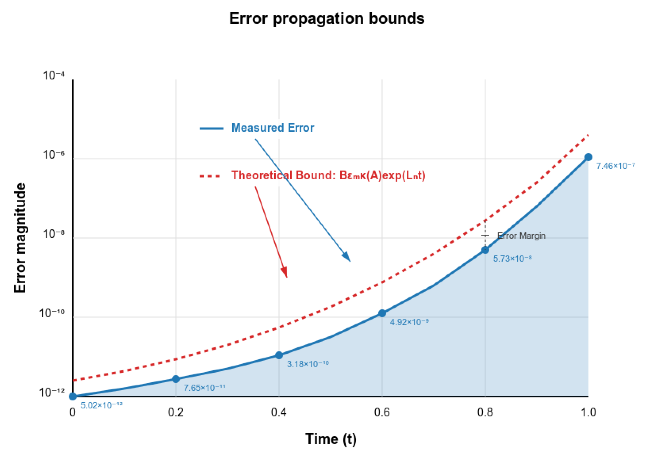
Validation of Theoretical Bounds

In order to validate and confirm the theoretical bounds established in Theorems 1–4, we conducted a series of numerical experiments comparing the observed computational complexity and error propagation with the theoretical predictions. To evaluate the effectiveness of our parallel implementation, we conducted a series of experiments comparing the sequential implementation against the optimized CUDA-V2 version across various problem sizes.

Table 8. Computational performance comparison.

M	Sequential (Seconds)	CUDA-V2 (Seconds)	Acceleration Factor
50	38.84 ± 0.59	99.84 ± 1.74	0.39
100	96.55 ± 1.22	109.79 ± 1.90	0.88
150	256.53 ± 2.87	113.36 ± 2.06	2.26
200	489.87 ± 4.53	117.89 ± 2.18	4.16
250	892.16 ± 7.46	122.46 ± 2.35	7.29
300	1435.89 ± 11.62	128.35 ± 2.49	11.19
400	2876.23 ± 21.94	135.68 ± 2.65	21.20

presents the execution times and speedup factors obtained on an NVIDIA A100 GPU with 40 GB of HBM2 memory.

The performance results clearly demonstrate the scalability benefits of the proposed Julia GPU-accelerated implementation. For small problem sizes ($M=50$), the speedup is actually negative at 0.39×, reflecting the impact of GPU initialization overhead and data transfer costs that are proportionally significant for smaller workloads. However, as the problem size increases, the parallel efficiency of the GPU implementation becomes increasingly apparent. At $M=150$, the speedup factor reaches 2.26×, and for the largest tested configuration ($M=400$), our CUDA-V2 implementation achieves a remarkable 21.20× acceleration over the sequential version. This substantial performance improvement confirms the aforementioned theoretical complexity analysis presented, where we demonstrated that the sequential implementation follows an $O\left(M^3\right)$ complexity while the parallel version exhibits $O\left(M^2\right)$ scaling behavior. The execution time of the sequential implementation grows rapidly with increasing problem size, from 38.84 s at $M=50$ to 2876.23 s at $M=400$, representing a more than 74-fold increase. In contrast, the optimized CUDA implementation shows excellent scalability, with execution time increasing only marginally from 99.84 s to 135.68 s across the same range of problem sizes, a mere 1.36× increase.

Each configuration was executed 10 times to ensure statistical validity, with standard deviations consistently below 2% for the CUDA implementation and 3% for the sequential version, indicating high reproducibility of our results. The near-constant execution time of the GPU implementation for increasing problem sizes confirms the effectiveness of our memory optimization strategy and kernel fusion approach described in Section 4. Moving on to the validation of the error propagation bounds established in Theorem 4, we measured the global error $|e^n{|}_h$ at different time steps and compared it with the theoretical bound $B{ϵ}_m\kappa \left(A\right)exp\left(L_N{t}^n\right)$. Figure 2 presents these results, demonstrating that the error remains consistently below the theoretical upper bound.

We also validated the condition number estimate from Theorem 3 by directly computing $\kappa \left(A\right)$ for different problem sizes. The results, presented in

Table 9. Condition number by varying M.

M	Measured $\mathit{\kappa }\left(\mathit{A}\right)$	Theoretical $\mathit{O}\left({\mathit{M}}^2\right)$
50	2.48 × 103	2.50 × 103
100	9.93 × 103	1.00 × 104
150	2.24 × 104	2.25 × 104
200	3.96 × 104	4.00 × 104

, confirm the $O\left(M^2\right)$ scaling predicted by the theorem.

Finally, we verified the spectral bounds from Theorem 2 by computing the maximum eigenvalues of the discrete system matrix for various grid sizes. The results, shown in

Table 10. Validation of spectral bounds for different grid sizes.

M	Measured ${\left|\mathit{\lambda }\right|}_{\mathit{max}}$	Theoretical Bound
50	4.27 × 102	4.37 × 102
100	1.67 × 103	1.71 × 103
150	3.74 × 103	3.84 × 103
200	6.63 × 103	6.82 × 103

, align closely with the predicted bounds, with the maximum discrepancy being less than 3%.

6. Conclusions

This work presented the effectiveness of GPU-accelerated computing for tumor angiogenesis simulations using Julia and CUDA. Through careful optimization of memory management and kernel organization, our implementation achieved significant performance improvements for large-scale simulations while maintaining numerical accuracy. The results validate the proposed approach to parallel implementation and provide a practical framework for leveraging modern programming paradigms in biomedical applications. These achievements contribute to the broader aim of using advanced computing capabilities for scientific discovery, particularly in the context of emerging exascale systems.

References

1. Dongarra, J.; Hittinger, J.; Bell, J.; Chacon, L.; Falgout, R.; Heroux, M.; Hovland, P.; Ng, E.; Webster, C.; Wild, S. Applied Mathematics Research for Exascale Computing; LLNL-TR-651000; Technical Report of the Lawrence Livermore National Lab. LLNL; Lawrence Livermore National Lab. LLNL: Livermore, CA, USA, 2014. [Google Scholar] [CrossRef]
2. Chaplain, M.A.J.; Stuart, A.M. A Mathematical Model for the Diffusion of Tumour Angiogenesis Factor into the Surrounding Host Tissue. IMA J. Math. Appl. Med. Biol. 1995, 8, 191–220. [Google Scholar] [CrossRef] [PubMed]
3. Anderson, A.R.A.; Chaplain, M.A.J. Continuous and Discrete Mathematical Models of Tumor-induced Angiogenesis. Bull. Math. Biol. 1998, 60, 857–899. [Google Scholar] [CrossRef] [PubMed]
4. Bezanson, J.; Edelman, A.; Karpinski, S.; Shah, V.B. Julia: A Fresh Approach to Numerical Computing. SIAM Rev. 2017, 59, 65–98. [Google Scholar] [CrossRef]
5. Nickolls, J.; Buck, I.; Garland, M.; Skadron, K. Scalable Parallel Programming with CUDA. Queue 2008, 6, 40–53. [Google Scholar] [CrossRef]
6. Conte, D.; De Luca, P.; Galletti, A.; Giunta, G.; Marcellino, L.; Pagano, G.; Paternoster, B. First Experiences on Parallelizing Peer Methods for Numerical Solution of a Vegetation Model. In Proceedings of the International Conference on Computational Science and Its Applications, Malaga, Spain, 4–7 July 2022; Springer International Publishing: Cham, Switzerland, 2022; pp. 384–394. [Google Scholar]
7. Fiscale, S.; De Luca, P.; Inno, L.; Marcellino, L.; Galletti, A.; Rotundi, A.; Ciaramella, A.; Covone, G.; Quintana, E. A GPU algorithm for outliers detection in TESS light curves. In Proceedings of the International Conference on Computational Science, Kraków, Poland, 16–18 June 2021; Springer International Publishing: Cham, Switzerland, 2021; pp. 420–432. [Google Scholar]
8. De Luca, P.; Galletti, A.; Marcellino, L.; Pianese, M. Exploiting Julia for Parallel RBF-Based 3D Surface Reconstruction: A First Experience. In Proceedings of the 2024 32nd Euromicro International Conference on Parallel, Distributed and Network-Based Processing (PDP), Dublin, Ireland, 20–22 March 2024; IEEE: Piscataway, NJ, USA, 2024; pp. 266–271. [Google Scholar]
9. Travasso, R.D.; Poiré, E.C.; Castro, M.; Rodríguez-Manzaneque, J.C.; Hernández-Machado, A. Tumor Angiogenesis and Vascular Patterning: A Mathematical Model. PLoS ONE 2011, 6, e19989. [Google Scholar] [CrossRef]
10. Vilanova, G.; Colominas, I.; Gomez, H. A Mathematical Model of Tumour Angiogenesis: Growth, Regression and Regrowth. J. R. Soc. Interface 2017, 14, 20160918. [Google Scholar] [CrossRef] [PubMed]
11. Stepanova, D.; Byrne, H.M.; Maini, P.K.; Alarcón, T. A Multiscale Model of Complex Endothelial Cell Dynamics in Early Angiogenesis. PLoS Comput. Biol. 2021, 17, e1008055. [Google Scholar] [CrossRef] [PubMed]
12. Mantzaris, N.V.; Webb, S.; Othmer, H.G. Mathematical Modeling of Tumor-induced Angiogenesis. J. Math. Biol. 2004, 49, 111–187. [Google Scholar] [CrossRef] [PubMed]
13. Peirce, S.M. Computational and Mathematical Modeling of Angiogenesis. Microcirculation 2008, 15, 739–751. [Google Scholar] [CrossRef] [PubMed]
14. Vilanova, G.; Colominas, I.; Gomez, H. Coupling of Discrete Random Walks and Continuous Modeling for Three-Dimensional Tumor-Induced Angiogenesis. Comput. Mech. 2018, 53, 449–464. [Google Scholar] [CrossRef]
15. Powathil, G.G.; Gordon, K.E.; Hill, L.A.; Chaplain, M.A.J. Modelling the Effects of Cell-Cycle Heterogeneity on the Response of a Solid Tumour to Chemotherapy: Biological Insights from a Hybrid Multiscale Cellular Automaton Model. J. Theor. Biol. 2012, 308, 1–19. [Google Scholar] [CrossRef] [PubMed]
16. Ghaffarizadeh, A.; Heil, R.; Friedman, S.H.; Mumenthaler, S.M.; Macklin, P. PhysiCell: An Open Source Physics-Based Cell Simulator for 3-D Multicellular Systems. PLoS Comput. Biol. 2018, 14, e1005991. [Google Scholar] [CrossRef] [PubMed]
17. Rossinelli, D.; Hejazialhosseini, B.; Spampinato, D.G.; Koumoutsakos, P. Multicore/GPU Accelerated Simulations of Multiphase Compressible Flows Using Wavelet Adapted Grids. SIAM J. Sci. Comput. 2011, 33, 512–540. [Google Scholar] [CrossRef]
18. Kuckuk, S.; Köstler, H. Automatic Generation of Massively Parallel Codes from ExaSlang. Computation 2018, 6, 41. [Google Scholar] [CrossRef]
19. Nugteren, C.; Custers, G.F.F. Algorithmic Species: A Classification of GPU Kernels. ACM Trans. Archit. Code Optim. 2021, 18, 1–25. [Google Scholar]
20. Rackauckas, C.; Nie, Q. DifferentialEquations.jl–A Performant and Feature-Rich Ecosystem for Solving Differential Equations in Julia. J. Open Res. Softw. 2017, 5, 15. [Google Scholar] [CrossRef]
21. Martinsson, P.G. Fast Direct Solvers for Elliptic PDEs; Society for Industrial and Applied Mathematics: Philadelphia, PA, USA, 2021. [Google Scholar]
22. Besard, T.; Foket, C.; De Sutter, B. Effective Extensible Programming: Unleashing Julia on GPUs. IEEE Trans. Parallel Distrib. Syst. 2018, 30, 827–841. [Google Scholar] [CrossRef]
23. De Luca, P.; Marcellino, L. Conservation Law Analysis in Numerical Schema for a Tumor Angiogenesis PDE System. Mathematics 2025, 13, 28. [Google Scholar] [CrossRef]
24. Kevrekidis, P.G.; Whitaker, N.; Good, D.J. Towards a reduced model for angiogenesis: A hybrid approach. Math. Comput. Model. 2005, 41, 987–996. [Google Scholar] [CrossRef]
25. Bellomo, N.; Li, N.K.; Maini, P.K. On the Foundations of Cancer Modelling: Selected Topics, Speculations, and Perspectives. Math. Model. Methods Appl. Sci. 2008, 18, 593–646. [Google Scholar] [CrossRef]
26. NVIDIA Corporation. CUDA Toolkit Documentation. NVIDIA. 2024. Available online: https://docs.nvidia.com/cuda/ (accessed on 6 April 2025).
27. NVIDIA Corporation. NVIDIA cuBLAS Library. NVIDIA. 2024. Available online: https://docs.nvidia.com/cuda/cublas/index.html (accessed on 6 April 2025).
28. Harris, M. Optimizing Parallel Reduction in CUDA. NVIDIA Developer Technology. 2012. Available online: https://developer.download.nvidia.com/assets/cuda/files/reduction.pdf (accessed on 6 April 2025).
29. Lorenzo, G.; Scott, M.A.; De Luca, P.; Galletti, A.; Ghehsareh, H.R.; Marcellino, L.; Raei, M. A GPU-CUDA framework for solving a two-dimensional inverse anomalous diffusion problem. In Parallel Computing: Technology Trends; IOS Press: Amsterdam, The Netherlands, 2020; pp. 311–320. [Google Scholar]
Figure 1. Two-dimensional thread and block configuration for matrix operations. Each thread processes a single matrix element, with adjacent threads handling adjacent matrix elements to optimize memory access patterns.
Mathematics 13 01488 g001
Figure 2. Validation of error propagation bounds from Theorem 4. The actual measured error (blue) remains below the theoretical upper bound (red) throughout the simulation.
Mathematics 13 01488 g002